BINARY CONTROL AND DIGITAL-TO-ANALOG CONVERSION USING COMPOSITE NUV PRIORS AND ITERATIVE GAUSSIAN MESSAGE PASSING

Abstract

The paper proposes a new method to determine a binary control signal for an analog linear system such that the state, or some output, of the system follows a given target trajectory. The method can also be used for digital-to-analog conversion.

The heart of the proposed method is a new binary-enforcing NUV prior (normal with unknown variance). The resulting computations, for each planning period, amount to iterating forward-backward Gaussian message passing recursions (similar to Kalman smoothing), with a complexity (per iteration) that is linear in the planning horizon. In consequence, the proposed method is not limited to a short planning horizon.

Index Terms—  Discrete-level priors, normals with unknown variance (NUV), finite-control-set model predictive control (MPC), digital-to-analog conversion (DAC).

1 Introduction

Consider the classical control problem of steering an analog physical linear system along some desired trajectory, or to make the system produce some desired analog output. In this paper, we are interested in the special case where the control input is binary (i.e., restricted to two levels), which makes the problem much harder. This binary-input control problem includes, in particular, a certain type of analog-to-digital converter where the binary output of some digital processor directly drives a continuous-time analog linear filter—preferably an inexpensive one—which produces the desired analog waveform.

It is tempting to ask for an optimal binary control signal, i.e., a control signal that produces the best approximation of the desired analog trajectory (e.g., for a quadratic cost function). However, determining such an optimal control signal is a hard combinatorial optimization problem, with a computational complexity growing exponentially with the planning horizon [1, 2]. In consequence, insisting on an optimal control signal limits us to a short planning horizon, which is a very severe restriction. This problem is well known in model predictive control (MPC) [3, 4]. Techniques such as sphere decoding do help [5], but the fundamental problem remains.

Clearly, the binary-input control problem is a nonconvex optimization problem. A general approach to nonconvex optimization is to resort to some convex relaxation, and to project the solution back to the permissible set [6]. Other general approaches include heuristic methods such as random-restart hill-climbing [7] and simulated annealing [8].

The heart of the method proposed in this paper is a new binary-enforcing NUV prior (normal with unknown variance). NUV priors are a central idea of sparse Bayesian learning [9, 10, 11, 12], and closely related to variational representations of Lp norms [13, 14]. Such priors have been used mainly for sparsity; in particular, no binary-enforcing NUV prior seems to have been proposed in the prior literature. (An interesting non-NUV binary-enforcing prior has been proposed in [15].)

A main advantage of NUV priors in general is their computational compatibility with linear Gaussian models, cf. [16]. In this paper, the computations (for each planning period) amount to iterating forward-backward Gaussian message passing recursions similar to Kalman smoothing, with a complexity (per iteration) that is linear in the planning horizon. In consequence, the proposed method can effectively handle long planning horizons, which can far outweigh its suboptimality.

2 The Binary-enforcing NUV Prior

Let $\mathcal{N}\!\left({x;\mu,\sigma^{2}}\right)$ denote the normal probability density function in $x$ with mean $\mu\in\mathbb{R}$ and variance $\sigma^{2}$. Let rCl ρ(x, θ) ≜N​(x; a, σ_1^2) N​(x; b, σ_2^2), where $\theta\triangleq(\sigma_{1}^{2},\sigma_{2}^{2})$ is a shorthand for the two unknown variances in (2). For fixed $\theta$, $\rho(x,\theta)$ is a normal probability density in $x$ (up to a scale factor), which is essential for the algorithms in Section 3.3.

The heart of the proposed method is the observation that (2) can be used as a (improper) joint prior for $x$ and $\theta$ that strongly encourages $x$ to lie in $\{a,b\}$. To see this, assume $\rho(x,\theta)$ is used in some model with (fixed) observation(s) $\breve{y}$ and likelihood function $p(\breve{y}\hskip 0.20004pt|\hskip 0.80002ptx)$. Two different ways to estimate the variances $\theta$ are considered in Sections 2.1 and 2.2. For the numerical examples in Figs. 3 and 3, we will assume that $p(\breve{y}\hskip 0.20004pt|\hskip 0.80002ptx)$ is Gaussian (in $x$) with mean $\mu$ and variance $s^{2}$ depending on $\breve{y}$, i.e.,

$$p(\breve{y}\hskip 0.20004pt|\hskip 0.80002ptx)=\mathcal{N}\!\left({x;\mu,s^{2}}\right).$$ (1)

A factor graph [17] of the resulting statistical system model

$$p(\breve{y}\hskip 0.20004pt|\hskip 0.80002ptx)\rho(x,\theta)=\mathcal{N}\!\left({x;\mu,s^{2}}\right)\mathcal{N}\!\left({x;a,\sigma_{1}^{2}}\right)\mathcal{N}\!\left({x;b,\sigma_{2}^{2}}\right)$$ (2)

is shown in Fig. 1.

Fig. 1: Factor graph of (2) for fixed $\breve{y}$. The boxes labeled “$\mathcal{N}$” represent normal probability density functions $\mathcal{N}\!\left({0,1}\right)$.

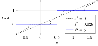
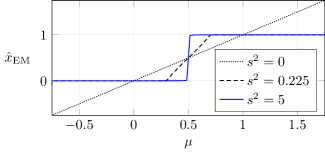
Fig. 2: The estimate of Section 2.1, for $a=0$ and $b=1$, as a function of $\mu$.

Fig. 3: The estimate of Section 2.2, for $a=0$ and $b=1$, as a function of $\mu$.

2.1 Joint MAP Estimation

Assume that $x$ and $\theta$ are determined by joint MAP estimation. The resulting estimate $\hat{x}$ of $x$ is rCl ^x & = argmax_x max_θ p(˘y  — x) ρ(x, θ)
= argmax_x p(˘y  — x) max_θ ρ(x, θ), with an effective (improper) prior rCl max_θ ρ(x, θ) & = max_σ_1^2 N​(x; a, σ_1^2) max_σ_2^2 N​(x; b, σ_2^2)
∝ 1—x-a—⋅—x-b— It is obvious that this effective prior has a strong preference for $x$ to lie in $\{a,b\}$.

Such estimates may conveniently be computed by alternating maximization (AM) over $x$ and $\theta$, cf. Section 3.3.2. However, AM may converge to a local maximum rather than the global maximum (2.1), in which case the estimate $\hat{x}_{\text{AM}}$ returned by AM may lie outside $\{a,b\}$.

For $p(\breve{y}\hskip 0.20004pt|\hskip 0.80002ptx)$ as in (1), the estimate $\hat{x}_{\text{AM}}$ is plotted in Fig. 3. In this setting, we observe (and it can be proved) that, for every fixed $\mu$ and sufficiently large $s^{2}$, there is no local maximum and $\hat{x}_{\text{AM}}$ lies in $\{a,b\}$.

2.2 Type-II Estimation

In this case, we first determine the MAP estimate $\hat{\theta}$ of $\theta$, i.e.,

$$\hat{\theta}=\operatorname*{argmax}_{\theta}\int_{-\infty}^{\infty}p(\breve{y}\hskip 0.20004pt|\hskip 0.80002ptx)\rho(x,\theta)\,dx,$$ (3)

and then we estimate $x$ as

$$\hat{x}=\operatorname*{argmax}_{x}p(\breve{y}\hskip 0.20004pt|\hskip 0.80002ptx)\rho(x,\hat{\theta}).$$ (4)

Such estimates may conveniently be computed by expectation maximization (EM) (cf. Section 3.3.3), which, however, may converge to a local maximum. Moreover, even the global maximum (4) may lie outside $\{a,b\}$. Nonetheless, for $p(\breve{y}\hskip 0.20004pt|\hskip 0.80002ptx)$ as in (1), we observe (and it can be proved) that, for every fixed $\mu\neq(a+b)/2$ and sufficiently large $s^{2}$, $\hat{x}_{\text{EM}}$ lies in $\{a,b\}$, as illustrated in Fig. 3.

3 System Model and Algorithms

3.1 Problem Statement

Consider a linear system with scalar input $u_{k}\in\mathbb{R}$ and state $x_{k}\in\mathbb{R}^{N}$, which evolves according to

$$x_{k}=Ax_{k-1}+Bu_{k},$$ (5)

where $k\in\{1,2,\ldots,K\}$ is the time index (with finite horizon $K$), and where both $A\in\mathbb{R}^{N\times N}$ and $B\in\mathbb{R}^{N\times 1}$ are assumed to be known. Our goal is to determine a two-level input signal $u_{1},\,\ldots,u_{K}\in\{a,b\}$ such that some output (or feature)

$$y_{k}=Cx_{k}\in\mathbb{R}^{L}$$ (6)

(with known $C\in\mathbb{R}^{L\times N}$) follows a given trajectory $\breve{y}_{1}$, …, $\breve{y}_{K}\in\mathbb{R}^{L}$, i.e., we wish

$$\sum_{k=1}^{K}\|y_{k}-\breve{y}_{k}\|^{2}$$ (7)

to be as small as possible. For ease of exposition, we will assume that the initial state $x_{0}$ is known.

Note that this offline control problem may be viewed as a single episode of an online control problem, with planning horizon $K$. Note also that we are primarily interested in $K\gg 1$, which precludes exhaustive tree search algorithms.

3.2 The Statistical Model

In order to solve the problem stated in Section 3.1, we turn it into a statistical estimation problem with an (improper) i.i.d. prior

$$\rho(u,\theta)\triangleq\prod_{k=1}^{K}\rho(u_{k},\theta_{k}),$$ (8)

where $u\triangleq(u_{1},\,\ldots,u_{K})$, $\theta\triangleq(\theta_{1},\,\ldots,\theta_{K})$, and

$$\rho(u_{k},\theta_{k})\triangleq\mathcal{N}\!\left({u_{k};a,\sigma_{1,k}^{2}}\right)\mathcal{N}\!\left({u_{k};b,\sigma_{2,k}^{2}}\right)$$ (9)

with $\theta_{k}=(\sigma_{1,k}^{2},\sigma_{2,k}^{2})$ as in (2). Accordingly, we replace (7) by the likelihood function

$$p(\breve{y}\hskip 0.20004pt|\hskip 0.80002ptu)=\prod_{k=1}^{K}\frac{1}{(2\pi)^{L/2}s^{L}}\exp\left(\frac{-\|y_{k}-\breve{y}_{k}\|^{2}}{2s^{2}}\right),$$ (10)

where $\breve{y}=(\breve{y}_{1},\,\ldots,\breve{y}_{K})$ and where $s>0$ is a free parameter. The complete statistical model is then given by

$$p(\breve{y},u,\theta)\triangleq p(\breve{y}\hskip 0.20004pt|\hskip 0.80002ptu)\rho(u,\theta)$$ (11)

together with (5) and (6).

3.3 Algorithms

Both joint MAP estimation of $u$ and $\theta$ (as in Section 2.1) and type-II estimation of $u$ and $\theta$ (as in Section 2.2) can be implemented as special cases (with different versions of Step 2) of the following algorithm.

3.3.1 Iterative Kalman Input Estimation (IKIE)

The algorithm estimates $\theta$ and $u$ by alternating the following two steps for $i=1,2,3,\,\ldots\,$:

1. For fixed $\theta=\theta^{(i-1)}$, compute the posterior means $\hat{u}_{k}^{(i)}$ of $u_{k}$ (for $k=1,\,\ldots,K$) and, if necessary, the posterior variances $V_{U_{k}}^{(i)}$ of $u_{k}$, with respect to the probability distribution $p(u\hskip 0.20004pt|\hskip 0.80002pt\breve{y},\theta)$.

2. From these means and variances, determine new NUV parameters $\theta^{(i)}$.

Note that Step 1 operates with a standard linear Gaussian model. In consequence, the required means and variances can be computed by standard Kalman-type recursions or, equivalently, by forward-backward Gaussian message passing, with a complexity that is linear in $K$.

A preferred such algorithm is MBF message passing as in [16, Section V], which amounts to Modified Bryson–Frazier smoothing [18] augmented with input signal estimation. This algorithm requires no matrix inversion and is numerically quite stable.

3.3.2 Determining $\theta$ and $u$ by Joint MAP Estimation

In this case, we wish to compute the estimate rCl ^u & = argmax_u max_θp(˘y  — u) ρ(u, θ). The double maximization (over $u$ and $\theta$) is naturally implemented by alternating maximization, which can be implemented by the IKIE algorithm, with Step 2 given by

$$\big{(}\sigma_{1,k}^{2}\big{)}^{(i)}=\big{(}\hat{u}_{k}^{(i)}\,-a\big{)}^{2}\text{~{}~{}and~{}~{}}\big{(}\sigma_{2,k}^{2}\big{)}^{(i)}=\big{(}\hat{u}_{k}^{(i)}\,-b\big{)}^{2}.$$ (12)

3.3.3 Type-II Estimation

In this case, we wish to compute the estimate

$$\hat{\theta}=\operatorname*{argmax}_{\theta}\int p(\breve{y}\hskip 0.20004pt|\hskip 0.80002ptu)\rho(u,\theta)\mathop{}\!\mathrm{d}u,$$ (13)

which can be carried out by expectation maximization [19] with hidden variable(s) $u$. The update step for $\theta$ is rCl θ^(i) &= argmax_θ $\mathbb{E}$​[logp(˘y  — U) ρ(U, θ)]
= argmax_θ $\mathbb{E}$​[logρ(U, θ)], where the expectation is with respect to $p(u\hskip 0.20004pt|\hskip 0.80002pt\breve{y},\theta^{(i-1)})$. The update (13) turns out to be computable by the IKIE algorithm with Step 2 given by rCl ( σ_1,k^2 )^(i) & = V_U_k^(i) + (^u_k^(i) - a )^2   and
( σ_2,k^2 )^(i) = V_U_k^(i) + (^u_k^(i) -b )^2 ​.

3.3.4 Remarks

1. The algorithms of this section normally converge to a local (not the global) maximum of (3.3.2) or (13).

2. The parameter $s$ controls the error (7). If $s$ is chosen too small, the algorithm may return a nonbinary $u$.

3. Type-II estimation empirically works better than joint MAP estimation (in agreement with [20]). The numerical results in Figs. 4 and 5 are obtained with type-II estimation.

4 Examples

4.1 Digital-to-Analog Conversion

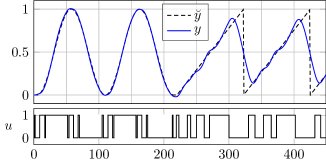
Fig. 4: Digital-to-analog conversion as in Section 4.1 with target waveform $\breve{y}$ (dashed), digital control signal $u$ (bottom), and filter output signal $y$ (solid blue).

One method for digital-to-analog conversion is to feed a continuous-time analog linear filter directly with a binary output signal $u$ of a digital processor. This method requires an algorithm to compute a suitable binary signal $u$ such that the analog filter output approximates the desired analog signal $\breve{y}$. A standard approach is to compute $u$ by a delta-sigma modulator [21], which requires the analog filter to approximate an ideal low-pass filter. By contrast, the method of this paper works also with simpler (i.e., less expensive) analog filters.

For the following numerical example, the analog filter is a 3rd-order low-pass, resulting in the discrete-time state space model rCl A &= [0.7967-6.3978-94.21230.0027 0.9902 -0.14670 0.0030 0.9999 ], $B=\begin{bmatrix}0.0027&0&0\end{bmatrix}^{{\mathsf{T}}}\!$, and $C=\begin{bmatrix}0&0&35037.9\end{bmatrix}$. The numerical results in Fig. 4 are obtained with $a=0$, $b=1$, $K=450$ and $s^{2}=0.045$.

4.2 Trajectory Planning with Sparse Checkpoints

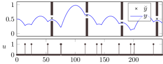
Fig. 5: Flappy bird control with check points $\breve{y}$, binary control signal $u$ (bottom), and resulting trajectory $y$ (solid blue).

The following control problem is a version of the flappy bird computer game [22]. Consider an analog physical system consisting of a point mass $m$ moving forward (left to right in Fig. 5) with constant horizontal velocity and “falling” vertically with constant acceleration $g$. The $\{0,1\}$-valued control signal $u$ affects the system only if $u_{k}=1$, in which case a fixed value is added to the vertical impulse. We wish to steer the point mass such that it passes approximately through a sequence of check points, as illustrated in Fig. 5.

For this example, we need a slight generalization of (5)–(7) as follows. The state $x_{k}\in\mathbb{R}^{2}$ (comprising the vertical position and the vertical speed) evolves according to rCl x_k & = [1 T 0 1 ]x_k-1 + [0 1/m ]u_k + [0 -Tg ], and we wish the vertical position $y_{k}=\begin{bmatrix}1&0\end{bmatrix}x_{k}$ to minimize

$$\sum_{k=1}^{K}w_{k}(y_{k}-\breve{y}_{k})^{2},$$ (14)

where $w_{k}=1$ if $\breve{y}_{k}$ is a checkpoint and $w_{k}=0$ otherwise.

The numerical results in Fig. 5 are obtained with $m=0.5$, $T=0.1$, $g=0.25$, $a=0$, $b=1$, $K=250$, and $s^{2}=0.1$.

5 Conclusion

We have proposed a new method for controlling a linear system with binary input, which can also be used for digital-to-analog conversion. The key idea is a new binary-enforcing prior with a NUV representation, which turns the actual computations into iterations of Kalman-type forward-backward recursions. The computational complexity of the proposed method is linear in the planning horizon, with compares favorably with existing “optimal” methods.

The proposed prior and method can be extended both to $M>2$ levels and to sparse level switching in the control signal, as will be detailed elsewhere.

The suitability of the proposed prior for other applications remains to be investigated.

References

- [1] A. H. Land and A. G. Doig, “An automatic method of solving discrete programming problems,” Econometrica, vol. 28, no. 3, pp. 497–520, 1960.
- [2] L. A. Wolsey and G. L. Nemhauser, Integer and Combinatorial Optimization. John Wiley & Sons, 1999.
- [3] R. P. Aguilera and D. E. Quevedo, “On stability and performance of finite control set MPC for power converters,” in IEEE Workshop on Predictive Control of Electrical Drives and Power Electronics, 2011, pp. 55–62.
- [4] T. Geyer and D. E. Quevedo, “Multistep finite control set model predictive control for power electronics,” IEEE Trans. Power Electron., vol. 29, no. 12, pp. 6836–6846, 2014.
- [5] T. Dorfling, H. du Toit Mouton, T. Geyer, and P. Karamanakos, “Long-horizon finite-control-set model predictive control with nonrecursive sphere decoding on an FPGA,” IEEE Trans. Power Electron., vol. 35, no. 7, pp. 7520–7531, 2020.
- [6] S. Sparrer and R. F. H. Fischer, “Adapting compressed sensing algorithms to discrete sparse signals,” in 18th International ITG Workshop on Smart Antennas, 2014, pp. 1–8.
- [7] S. Russel and P. Norvig, Artificial intelligence: A modern approach. Pearson Education Limited, 2013.
- [8] M. Pincus, “Letter to the editor – a Monte Carlo method for the approximate solution of certain types of constrained optimization problems,” Operations Research, vol. 18, no. 6, pp. 1225–1228, 1970.
- [9] M. E. Tipping, “Sparse Bayesian learning and the relevance vector machine,” Journal of Machine Learning Research, vol. 1, pp. 211–244, 2001.
- [10] M. E. Tipping and A. C. Faul, “Fast marginal likelihood maximisation for sparse Bayesian models,” in Proc. of the Ninth International Workshop on Artificial Intelligence and Statistics, 2003, pp. 3–6.
- [11] D. P. Wipf and B. D. Rao, “Sparse Bayesian learning for basis selection,” IEEE Trans. Signal Process., vol. 52, no. 8, pp. 2153–2164, 2004.
- [12] D. P. Wipf and S. S. Nagarajan, “A new view of automatic relevance determination,” in Advances in Neural Information Processing Systems, 2008, pp. 1625–1632.
- [13] H.-A. Loeliger, B. Ma, H. Malmberg, and F. Wadehn, “Factor graphs with NUV priors and iteratively reweighted descent for sparse least squares and more,” in Proc. Int. Symp. Turbo Codes & Iterative Inform. Process. (ISTC), 2018, pp. 1–5.
- [14] F. Bach, R. Jenatton, J. Mairal, and G. Obozinski, “Optimization with sparsity-inducing penalties,” Foundations and Trends in Machine Learning, vol. 4, no. 1, pp. 1–106, 2012.
- [15] J. Dai, A. Liu, and H. C. So, “Sparse Bayesian learning approach for discrete signal reconstruction,” 2019, unpublished, arXiv:1906.00309.
- [16] H.-A. Loeliger, L. Bruderer, H. Malmberg, F. Wadehn, and N. Zalmai, “On sparsity by NUV-EM, Gaussian message passing, and Kalman smoothing,” in Information Theory and Applications Workshop (ITA), La Jolla, CA, 2016, pp. 1–10.
- [17] H.-A. Loeliger, “An introduction to factor graphs,” IEEE Signal Process. Mag., vol. 21, no. 1, pp. 28–41, 2004.
- [18] G. J. Bierman, Factorization Methods for Discrete Sequential Estimation. Academic Press, 1977, vol. 128.
- [19] P. Stoica and Y. Selén, “Cyclic minimizers, majorization techniques, and the expectation-maximization algorithm: a refresher,” IEEE Signal Proc. Mag., vol. 21, no. 1, pp. 112–114, 2004.
- [20] R. Giri and B. Rao, “Type I and type II Bayesian methods for sparse signal recovery using scale mixtures,” IEEE Trans. on Signal Process., vol. 64, no. 13, pp. 3418–3428, 2016.
- [21] B. E. Boser and B. A. Wooley, “The design of sigma-delta modulation analog-to-digital converters,” IEEE J. Solid-State Circuits, vol. 23, no. 6, pp. 1298–1308, 1988.
- [22] Flappy Bird. Accessed 09-October-2020. [Online]. Available: https://en.wikipedia.org/wiki/Flappy_Bird