Huaqing Jin and Guosheng Yin^∗

Abstract. In clinical trials, there often exist multiple historical studies for the same or related treatment investigated in the current trial. Incorporating historical data in the analysis of the current study is of great importance, as it can help to gain more information, improve efficiency, and provide a more comprehensive evaluation of treatment. Enlightened by the unit information prior (UIP) concept in the reference Bayesian test, we propose a new informative prior called UIP from an information perspective that can adaptively borrow information from multiple historical datasets. We consider both binary and continuous data and also extend the new UIP methods to linear regression settings. Extensive simulation studies demonstrate that our method is comparable to other commonly used informative priors, while the interpretation of UIP is intuitive and its implementation is relatively easy. One distinctive feature of UIP is that its construction only requires summary statistics commonly reported in the literature rather than the patient-level data. By applying our UIP methods to phase III clinical trials for investigating the efficacy of memantine in Alzheimer’s disease, we illustrate its ability of adaptively borrowing information from multiple historical datasets in the real application.

KEY WORDS: Bayesian design; Clinical trial; Fisher’s information; Historical data; Informative prior; Multiple studies.

1 Introduction

Prior distributions are crucial in Bayesian data analysis and inference. By incorporating many sources of knowledge, such as expert opinions and historical data, a properly elicited prior distribution can help to analyze the current data more efficiently and thus reduce the cost and ethical hazard in clinical trials. With a large number of subjects followed for a long period of time, large-scale clinical trials are typically expensive and suffer from high ethical risk. Clinical trials are rarely conducted in isolation, and thus it is critical to combine multiple samples systematically to improve the analysis of the current study. For example, several cancer clinical trials on the same or similar types of treatment are often conducted with patients of different ethnicity groups or disease sub-types and sometimes in different countries (Brahmer et al., 2015; Borghaei et al., 2015; Wu et al., 2019). These trials typically have comparable settings, e.g., using the same endpoints with similar follow-ups and eligibility criteria, hence information can be borrowed across them to improve efficiency. It may also happen that trials investigate different treatments, while the same control arm is used (Borghaei et al., 2015; Rittmeyer et al., 2017), and thus the data in the control arm are valuable to the current trial as a common benchmark for comparison.

A major challenge associated with multiple historical datasets is to determine the amount of information borrowed from each dataset for the current study. Differences in patient populations or other trial-specific settings lead to heterogeneity among the current trial and historical trials, and thus the full-borrowing strategy is typically imprudent, as it would inflate the type I error substantially. Moreover, when the total sample size of the historical datasets is large, the information from historical datasets might overwhelm the analysis of the current study which is not desirable, as the data from the current study should typically dominate the analysis.

Several methods have been proposed for adaptively borrowing information from historical data. Pocock (1976) considers the difference in the parameters of interest between the current and historical datasets and models this difference with a zero-mean random variable. Ibrahim et al. (2000) propose the joint power prior (JPP) to discount the historical dataset by a power parameter in the range of $[0,1]$. Duan et al. (2006) and Neuenschwander et al. (2009) modify the JPP by adding a normalization term, which is referred to as the modified power prior (MPP). Banbeta et al. (2019) and Gravestock and Held (2019) further extend the power prior to multiple historical datasets with binary endpoints. Using a hierarchical model for the between-trial heterogeneity, Neuenschwander et al. (2010) develop the meta-analytic-predictive (MAP) prior via deriving the predictive distribution of the model parameter resulting from the analysis of the historical datasets. To further account for the prior-data conflict, Schmidli et al. (2014) make the MAP prior more robust by incorporating a noninformative component in the prior distribution (Weber et al., 2019) which is called robust MAP (rMAP). Hobbs et al. (2011) propose the commensurate prior by using the commensurate parameter directly to parameterize the commensurability between the historical and current data. There are also shrinkage estimation methods to borrow information from historical data (Röver and Friede, 2020a; Röver and Friede, 2020b), which are under the hierarchical model framework. All the aforementioned methods can borrow information according to the consistency between the historical and current datasets. Nonetheless, Pocock’s method and the commensurate prior are typically applicable to the case with a single historical dataset. When multiple historical datasets exist, the naive extensions for both methods do not take the underlying correlation among historical datasets into consideration. For the commensurate prior, when multiple historical datasets are involved, the formula under the non-Gaussian case would be complicated which causes difficulty in practice and the interpretations of multiple commensurate parameters may not be intuitive as the commensurability concept defined by Hobbs et al. (2011) is typically for the case with a single historical dataset. The MAP prior relies on the exchangeability assumption and adopts a single parameter to parameterize the heterogeneity between the current and historical datasets. With a single parameter, the relative contributions of historical datasets are not accounted for, i.e., heterogeneity of the coherence between the current and each historical dataset cannot be incorporated.

Kass and Wasserman (1995) use the Fisher information to define the amount of information and set the amount of information in the prior equal to that of a single observation to conduct Bayesian hypothesis tests using Bayes factors. Motivated by the information in a single observation, we propose the unit information prior (UIP) as a new class of informative prior distributions to dynamically borrow information from multiple historical datasets. Unlike other methods which are constructed from the likelihood function of historical datasets, the UIP is constructed from the information perspective and parameterizes the amount of Fisher information in the prior distribution directly. The amount of information in the UIP is closely related to the effective sample size (ESS) defined by Morita et al. (2008), and thus the UIP framework can straightforwardly control the ESS in the prior distribution. Moreover, our method considers the heterogeneity between the current and historical datasets separately which guarantees the efficiency of information borrowing. As it is elicited based on the Fisher information, often it only requires summary statistics of the historical data commonly reported in publications (e.g., point estimates and 95% confidence intervals) rather than the patient-level data. The UIP is easy to implement with multiple historical datasets, whose parameters have intuitive interpretations.

The rest of this paper is organized as follows. In Section 2, we introduce the general framework of the UIP methods. In Section 3, we illustrate the UIP framework under the single-arm trial with binary and continuous data respectively, and discuss its connection with the power prior, commensurate prior and MAP prior in terms of the conditional prior distribution as well as making an extension of the UIP to linear models. We also discuss the effective sample size (ESS) in the UIP (Morita et al., 2008, 2012). Extensive simulation studies are presented in Section 4 where we demonstrate the dynamic borrowing property of the UIP, and compare different priors for multiple historical datasets. Section 5 provides an example from six phase III clinical trials for Alzheimer’s disease which illustrates the behavior of our UIP approach in the real data application. We conclude the article with a brief discussion in Section 6.

2 Unit Information Prior

Let $D=\{Y_{1},\ldots,Y_{n}\}$ denote the data of the current trial of sample size $n$. Suppose that there are $K$ historical datasets $\{D_{1},\ldots,D_{K}\}$ related to the current study, where $D_{k}=\{Y_{k,1},\ldots,Y_{k,n_{k}}\}$ denotes the $k$th dataset of size $n_{k}$, for $k=1,\ldots,K$. The parameter of interest is often the treatment effect, denoted by $\theta$, for the current study, while the counterpart of $\theta$ for $D_{k}$ is denoted as $\theta_{k}$ for $k=1,\ldots,K$. The likelihood function of $\theta_{k}$ based on $D_{k}$ is denoted by $L^{(k)}(\theta_{k}|D_{k})$.

The UIP is constructed directly from an information perspective under the normal approximation. When eliciting an informative prior for the parameter of interest $\theta$, we are mainly interested in the accuracy and precision, i.e., the correctness and the amount of information contained in the prior distribution. Under the normal approximation, the accuracy of the prior distribution is determined by the mean of the prior and the amount of the Fisher information in the prior is the inverse of the variance. Thus, the UIP framework focuses on the mean and variance of the prior distribution, and the amount of information in the prior distribution can be explicitly controlled. Moreover, as UIP only requires the first and second moments, often the summary statistics of the historical data (e.g., mean and variance) would be sufficient to derive the prior distribution, which is the typical case in practice as the patient-level historical datasets are not easy to obtain.

When considering information borrowing from historical datasets, the parameter of interest $\theta$ is assumed to be close to the counterpart of historical datasets $\theta_{k}$. Due to heterogeneity among historical datasets, we introduce a weight parameter $w_{k}$ for the historical dataset $D_{k}$ to measure the relative closeness between the current dataset $D$ and the historical one $D_{k}$. The mean of the prior is defined as $\sum_{k=1}^{K}w_{k}\theta_{k}$, with the weight parameter $w_{k}\in(0,1)$ and $\sum_{k=1}^{K}w_{k}=1$, where $w_{k}$ can be also viewed as the measurement of the relative contribution from dataset $D_{k}$ to the analysis of the current study. The larger value of $w_{k}$, the more contribution from $D_{k}$.

Following the work of Kass and Wasserman (1995), we adopt the Fisher information as the measurement of the amount of information in the data. As a result, we define the unit information (UI) for $\theta_{k}$ in the dataset $D_{k}$ as

$$\mathrm{I}_{\mathrm{U}}(\theta_{k})=-\frac{1}{n_{k}}\frac{\partial^{2}\log L^{(k)}(\theta_{k}|D_{k})}{\partial\theta_{k}^{2}},$$

i.e., $\mathrm{I}_{\mathrm{U}}(\theta_{k})$ is the observed Fisher information of $D_{k}$ averaged at a unit observation level. When taking the heterogeneity of the historical datasets into consideration, the contribution of each historical dataset to the current study should be distinct. Therefore, the unit information from all the $K$ historical datasets is defined as $\sum_{k=1}^{K}w_{k}\mathrm{I}_{\mathrm{U}}(\theta_{k})$. We introduce $M$ as the sample size of the total amount of information borrowed from the $K$ datasets, and then the amount of information contained in the prior is $M\sum_{k=1}^{K}w_{k}\mathrm{I}_{\mathrm{U}}(\theta_{k})$. Under the normal approximation, the variance of the prior distribution is $\left\{M\sum_{k=1}^{K}w_{k}\mathrm{I}_{\mathrm{U}}(\theta_{k})\right\}^{-1}$.

Therefore, to adaptively borrow information from different datasets, we formulate the UIP framework as follows,

$$\theta|(M,w_{1},\ldots,w_{K},D_{1},\ldots,D_{K}) \sim \pi(\theta|M,w_{1},\ldots,w_{K},D_{1},\ldots,D_{K}),$$

$$\mathrm{with}\quad\mathbb{E}_{\pi}(\theta) = \sum_{k=1}^{K}w_{k}\theta_{k},$$

$$\mbox{Var}_{\pi}(\theta) = \left\{M\sum_{k=1}^{K}w_{k}\mathrm{I}_{\mathrm{U}}(\theta_{k})\right\}^{-1}.$$

As $\theta_{k}$ is typically unknown, we adopt the maximum likelihood estimator (MLE) $\hat{\theta}_{k}$ to replace $\theta_{k}$ while keeping $M,w_{1},\ldots,w_{K}$ as unknown parameters that are determined adaptively by the data. We choose the MLE as the estimate of $\theta_{k}$ for its desirable properties (Hunter, 2014), e.g., consistency and asymptotic efficiency. Moreover, in many cases, the MLE is simply the mean of the samples which can be easily obtained.

The specific form of $\pi$ depends on the parameter of interest $\theta$. For example, if $\theta$ is the mean parameter of a normal distribution, the UIP of $\theta$ can have a normal distribution; and if $\theta$ is the rate parameter of a Bernoulli distribution, the UIP of $\theta$ may conform to a Beta distribution.

The parameter $M$ determines the total number of units corresponding to the amount of information borrowed from all historical datasets as a whole. It is shown that the value of $M$ is closely related to the ESS defined by Morita et al. (2008). In practice, $M$ can be either fixed when we aim to control the amount of information borrowed from historical data or unknown by setting a hyper-prior on $M$. When there is a lack of prior information on $M$, a noninformative uniform prior is recommended as it is a standard practice in Bayesian methods; otherwise, Gamma or Poisson distribution can be used to incorporate the prior information of $M$ in the hyper-prior. For the simulation studies, unless otherwise specified, we set a Uniform$(0,\sum_{k=1}^{K}n_{k})$ as the hyper-prior for $M$, i.e., the value of $M$ cannot exceeds the combined sample size of all historical datasets. If the total sample size of historical datasets is too large compared to the sample size of the current study, it is suggested to set the upper bound of Uniform distribution at $n$, the sample size of the current dataset.

It is essential to determine the values of weight parameters which characterize the amount of information borrowed from each historical dataset. The values of $w_{k}$’s reveal the relative importance of historical datasets. If one historical dataset is more consistent with the current study compared with the others, the corresponding weight parameter should be larger. Furthermore, the absolute weight $Mw_{k}$ can be interpreted as the number of units of information borrowed from historical dataset $D_{k}$. Therefore, the amount of information borrowing from different datasets mainly relies upon the weight parameters, and the total amount of information borrowed from all historical datasets is determined by $M$.

We propose two approaches to determining the values of the weight parameters. One is a fully Bayesian approach by imposing a hyper-prior on $(w_{1},\ldots,w_{K})$. As all the values of $w_{k}$’s are between $0$ and $1$ satisfying the constraint $\sum_{k=1}^{K}w_{k}=1$, it is natural to assign a Dirichlet prior to $(w_{1},\ldots,w_{K})$. We take the sample sizes of historical datasets into consideration by selecting suitable parameters for the Dirichlet distribution. Intuitively, it is preferable to assign a higher weight to the historical dataset with larger sample size, while we should also prevent a historical dataset with extremely large sample size from dominating the information borrowing. To strike a balance, we recommend to set the hyper-prior for $(w_{1},\ldots,w_{K})$ as Dirichlet$(\gamma_{1},\ldots,\gamma_{K})$ where $\gamma_{k}=\min(1,{n_{k}}/{n})$. We refer to the UIP with a Dirichlet prior distribution as UIP-Dirichlet.

The other approach is to first measure the distances between the current dataset and the historical ones. To determine the values of weight parameters, a proper measure of the “distance” between two datasets is needed for measuring their similarity. The Jensen–Shannon (JS) divergence is a commonly used metric for measuring the dissimilarity between two probability distributions (Itzkovitz et al., 2010; Sims et al., 2009; Goodfellow et al., 2014). An alternative is the Kullback–Leibler (KL) divergence, while we adopt the JS divergence due to its symmetry property.

Similar to the discussion in the UIP-Dirichlet method, the weight parameter $w_{k}$ should tend to be small when the sample size of $D_{k}$ is small, while $w_{k}$ should not be too large even if the sample size of $D_{k}$ is extremely large. The JS divergence automatically penalizes the relatively small sample size (compared with the current dataset) of the historical dataset. When the sample size of $D_{k}$ is larger than that of the current dataset, we randomly select $n$ samples from $D_{k}$ to calculate the JS divergence and repeat this procedure for a large number of times to obtain the average. More specifically, the weight parameters are determined as follows.

1. Specify an initial non-informative prior (e.g., Jeffreys prior) for the parameter $\theta$ under the current dataset $D$ and $\theta_{k}$ under each $D_{k}$. Based on the initial prior, we obtain the initial posteriors $f_{\mathrm{ini}}(\theta|D)$.

2. For $k=1,\ldots,K$, when $n_{k}\leq n$, obtain the initial posterior $f_{\mathrm{ini}}(\theta|D_{k})$ and calculate the JS divergence

   $$d_{k}=\mathrm{JS}(D|D_{k})=\frac{\mathrm{KL}(D|D_{k})+\mathrm{KL}(D_{k}|D)}{2},$$

   where $\mathrm{KL}(D|D_{k})$ represents the KL divergence between two density functions $f_{\mathrm{ini}}(\theta|D)$ and $f_{\mathrm{ini}}(\theta|D_{k})$,

   $$\mathrm{KL}(D|D_{k})=\int f_{\mathrm{ini}}(\theta|D)\log\left\{\frac{f_{\mathrm{ini}}(\theta|D)}{f_{\mathrm{ini}}(\theta|D_{k})}\right\}\mathop{}\!\mathrm{d}\theta.$$

   When $n_{k}>n$, randomly draw $n$ samples from $D_{k}$ for $N$ times to obtain $\{D_{k}^{(l)}\}_{l=1}^{N}$ and compute the initial posteriors $\{f_{\mathrm{ini}}(\theta|D_{k}^{(l)})\}_{l=1}^{N}$, then calculate the distance $d_{k}$ as the average ${\sum_{l=1}^{N}\mathrm{JS}(D|D_{k}^{(l)})}/{N}$.

3. The weight parameters are defined as

   $$w_{k}=\frac{1/d_{k}}{\sum_{s=1}^{K}(1/d_{s})}$$

   for $k=1,\ldots,K$.

In extremely rare cases, $D$ and $D_{k}$ may be exactly the same which results in the zero JS divergence. As a remedy, we add a small number, say $10^{-6}$, to the $d_{k}$ to avoid the division-by-zero problem. We refer to the UIP in conjunction with the JS divergence as UIP-JS, where the weights are prespecified and the only unknown parameter is $M$ in the UIP-JS.

It is also possible to use other methods (e.g., the empirical Bayes method) to pre-determine the weight parameters before sampling. However, in terms of the computation, the JS divergence is easier compared with the empirical Bayes method. Moreover, the JS divergence measures the dissimilarity between two datasets from an information perspective, which is consistent with the UIP framework for the prior elicitation.

3 UIP with Binary and Continuous Data

We illustrate the UIP methods in a single-arm trial with continuous and binary data respectively. We also discuss the connections among the power prior, commensurate prior, MAP prior and UIP for continuous data in terms of the conditional prior distribution, as well as extending our UIP to linear models. Moreover, the relationship between the amount parameter $M$ and the ESS of the informative prior distribution is investigated.

3.1 Continuous Data

Suppose that $\{Y_{1},\ldots,Y_{n}\}$ are independent and identically distributed (i.i.d.) from $N(\theta,\sigma^{2})$ and $\{Y_{k,1},\ldots,Y_{k,n_{k}}\}$ are i.i.d. from $N(\theta_{k},\sigma^{2}_{k})$ for $k=1,\ldots,K$. The parameter of interest is the mean $\theta$ and the unit information for $D_{k}$ evaluated at the corresponding MLE $\hat{\theta}_{k}$ (which is the sample mean) is

$$\mathrm{I}_{\mathrm{U}}(\hat{\theta}_{k})=\frac{1}{\sigma^{2}_{k}}.$$

We impose an inverse-Gamma prior for $\sigma^{2}$, e.g., $\sigma^{2}\sim\mathrm{InvGa}(0.01,0.01)$. If the calculation involves $\sigma^{2}_{k}$, we simply replace $\sigma^{2}_{k}$ with its MLE $\hat{\sigma}^{2}_{k}$. As a result, we obtain the UIP as

$$\theta|(M,w_{1},\ldots,w_{K},D_{1},\ldots,D_{K}) \sim N(\mu,\eta^{2}),$$

where

$$\mu = \sum_{k=1}^{K}w_{k}\hat{\theta}_{k},$$

$$\eta^{2} = \left(M\sum_{k=1}^{K}\frac{w_{k}}{\hat{\sigma}^{2}_{k}}\right)^{-1}.$$

Under the normal distribution setting, the MPP, local commensurate prior (LCP), MAP prior and UIP are closely related as shown in formula (3.1). We extend the MPP to the case with multiple historical datasets as follows,

$$\pi^{\mathrm{MPP}}(\theta|\alpha_{1},\ldots,\alpha_{K},D_{1},\ldots,D_{K}) \propto \pi^{\mathrm{ini}}(\theta)\prod_{k=1}^{K}L^{(k)}(\theta|D_{k})^{\alpha_{k}},$$

$$\alpha_{k} \sim \mathrm{Beta}(a,b),\ k=1,\ldots,K,$$

$$\sigma^{2} \sim \mathrm{InvGa}(\zeta,\zeta),$$

$$\pi^{\mathrm{ini}}(\theta) \propto 1,$$

where $\alpha_{k}$ is the power parameter for $D_{k}$ and $\pi^{\mathrm{ini}}$ is the initial prior.

We also extend the LCP method to the case with $K$ historical datasets. Denoting the commensurate parameter for dataset $D_{k}$ by $\tau_{k}$, the LCP is given by

$$\pi^{\mathrm{LCP}}(\theta|\tau_{1},\ldots,\tau_{K},D_{1},\ldots,D_{K}) \propto \pi^{\mathrm{ini}}(\theta)\prod_{k=1}^{K}\int L^{(k)}(\theta_{k}|D_{k})N\big{(}\theta;\theta_{k},\frac{1}{\tau_{k}}\big{)}\mathop{}\!\mathrm{d}\theta_{k},$$

$$\log(\tau_{k}) \sim \mathrm{Unif}(\xi_{1},\xi_{2}),\ k=1,\ldots,K,$$

$$\sigma^{2} \sim \mathrm{InvGa}(\zeta,\zeta),$$

$$\pi^{\mathrm{ini}}(\theta) \propto 1.$$

Denoting the between-trial standard deviation as $\tau$, the MAP prior with multiple historical datasets can be written as

$$\theta_{1},\ldots,\theta_{K},\theta|\mu^{\mathrm{MAP}},\tau \sim N(\mu^{\mathrm{MAP}},\tau^{2}),$$

$$\pi(\mu^{\mathrm{MAP}}) \propto 1,$$

$$\tau \sim \mathrm{HN}(0,1),$$

where $\mathrm{HN}$ denotes the half-normal distribution.

The MPP and LCP respectively use the power parameter $\alpha_{k}$ and the commensurate parameter $\tau_{k}$ as the measurement of consistency between the current dataset and each historical dataset $D_{k}$. The MAP prior adopts the exchangeability assumption and utilizes a single between-trial dispersion parameter $\tau$ to measure the heterogeneity among the current and historical datasets. In the UIP methods, the weight parameters measure the relative consistency of the historical datasets with respect to the current dataset, while the total amount parameter $M$ measures the overall information borrowed from historical data.

Given the corresponding hyper-parameters, the specific forms of the MPP, LCP, MAP and UIP methods for continuous data are given as follows:

$$\pi^{\mathrm{MPP}}(\theta|\alpha_{1},\ldots,\alpha_{K},D_{1},\ldots,D_{K}) \sim N\left(\sum_{k=1}^{K}\frac{\alpha_{k}n_{k}/\hat{\sigma}_{k}^{2}}{\sum_{s=1}^{K}\alpha_{s}n_{s}/\hat{\sigma}^{2}_{s}}\hat{\theta}_{k},\left(\sum_{k=1}^{K}\alpha_{k}n_{k}\frac{1}{\hat{\sigma}^{2}_{k}}\right)^{-1}\right),$$

$$\pi^{\mathrm{LCP}}(\theta|\tau_{1},\ldots,\tau_{K},D_{1},\ldots,D_{K}) \sim N\left(\sum_{k=1}^{K}\frac{n_{k}\tau_{k}/(\tau_{k}\hat{\sigma}^{2}_{k}+n_{k})}{\sum_{s=1}^{K}n_{s}\tau_{s}/(\tau_{s}\hat{\sigma}^{2}_{s}+n_{s})}\hat{\theta}_{k},\left(\sum_{k=1}^{K}\frac{n_{k}\tau_{k}\hat{\sigma}_{k}^{2}}{\tau_{k}\hat{\sigma}^{2}_{k}+n_{k}}\frac{1}{\hat{\sigma}_{k}^{2}}\right)^{-1}\right),$$

$$\pi^{\mathrm{MAP}}(\theta|D_{1},\ldots,D_{K},\tau) \sim N\left(\sum_{k=1}^{K}\frac{n_{k}/(\hat{\sigma}_{k}^{2}+n_{k}\tau)}{\sum_{s=1}^{K}n_{s}/(\hat{\sigma}_{s}^{2}+n_{s}\tau)}\hat{\theta}_{k},\frac{1}{\sum_{k=1}^{K}n_{k}/(\hat{\sigma}_{k}^{2}+n_{k}\tau)}+\tau^{2}\right)$$

$$\pi^{\mathrm{UIP}}(\theta|M,w_{1},\ldots,w_{K},D_{1},\ldots,D_{K}) \sim N\left(\sum_{k=1}^{K}w_{k}\hat{\theta}_{k},\left(\sum_{k=1}^{K}w_{k}M\frac{1}{\hat{\sigma}_{k}^{2}}\right)^{-1}\right).$$ (3.1)

Conditioning on the hyper-parameters, the MPP, LCP, MAP and UIP approaches all lead to normal distributions with different means and variances. Interestingly, the means of all four priors can be written in a form of a weighted sum of the individual sample means. The UIP adopts weight parameters in a much more direct way, while the MPP parameterizes weights as an increasing function of the power parameters. The LCP method utilizes commensurate parameters $\tau_{k}$ to measure the commensurability between the current and historical datasets, where a larger value of $\tau_{k}$ indicates a higher level of commensurability, and the weight naturally increases with $\tau_{k}$. The MAP prior utilizes a single dispersion parameter $\tau$ to control the information borrowing, thus weight parameters mainly rely on the historical variances other than the dispersion parameter $\tau$.

The precision (i.e., the inverse of the variance) of the four priors can be used to quantify the amount of information borrowed from historical datasets. In particular, the precision of the MPP, LCP and UIP methods can be written as a weighted sum of the observed Fisher information from each dataset. For the MPP method, the number of units of information for $D_{k}$ is determined by the product of the corresponding power parameter $\alpha_{k}$ and the sample size $n_{k}$. The LCP approach adopts an increasing function of $\tau_{k}$ and $n_{k}$ as the amount of information borrowed from $D_{k}$. The amount of information from $D_{k}$ under the UIP framework corresponds to the product of the weight parameter $w_{k}$ and the total amount parameter $M$, which has the most transparent form and intuitive interpretation. Under the exchangeability assumption, the MAP prior borrows information from multiple historical datasets as a whole where the amount of information borrowed is a decreasing function of the dispersion parameter $\tau$.

3.2 Binary Data

Suppose that $\{Y_{1},\ldots,Y_{n}\}$ are i.i.d. samples from $\mathrm{Bernoulli(\theta)}$, while $\{Y_{k,1},\ldots,Y_{k,n_{k}}\}$ are those from $\mathrm{Bernoulli}(\theta_{k})$ for $k=1,\ldots,K$. The UI under the $k$th historical dataset $D_{k}$ evaluated at $\hat{\theta}_{k}$ is

$$\mathrm{I}_{\mathrm{U}}(\hat{\theta}_{k})=\frac{1}{\hat{\theta}_{k}(1-\hat{\theta}_{k})}.$$

As the support of the rate parameter $\theta$ is $[0,1]$, we assign a Beta prior on $\theta$. Denote the prior mean and prior variance of UIP as $\mu=\sum_{k=1}^{K}w_{k}\hat{\theta}_{k}$ and $\eta^{2}=\left\{M\sum_{k=1}^{K}{w_{k}}/\{\hat{\theta}_{k}(1-\hat{\theta}_{k})\}\right\}^{-1}$. Thus, the UIP of $\theta$ can be written as

$$\theta|(M,w_{1},\ldots,w_{K},D_{1},\ldots,D_{K}) \sim \mathrm{Beta}(\alpha,\beta),$$

where the two Beta distribution parameters can be easily derived by solving the mean and variance equations,

$$\alpha = \mu\left\{\frac{\mu(1-\mu)}{\eta^{2}}-1\right\},$$

$$\beta = (1-\mu)\left\{\frac{\mu(1-\mu)}{\eta^{2}}-1\right\}.$$

3.3 Linear Regression

Under a linear regression model, $Y_{i}\sim N({\bf x}_{i}^{\rm\top}\bm{\beta},\sigma^{2})$, where $\bm{\beta}=(\beta_{0},\ldots,\beta_{p})^{\rm\top}$ is the regression coefficients and ${\bf x}_{i}=(1,x_{1,i},\ldots,x_{p,i})^{\rm\top}$ is the covariate vector associated with the outcome $Y_{i}$. For the $k$th historical dataset, $Y^{(k)}_{i}\sim N({\bf x}_{i}^{(k)\top}\bm{\beta}^{(k)},\sigma_{k}^{2})$, where $\bm{\beta}^{(k)}=(\beta_{0}^{(k)},\ldots,\beta_{p}^{(k)})^{\rm\top}$ and ${\bf x}^{(k)}_{i}=(1,x_{1,i}^{(k)},\ldots,x_{p,i}^{(k)})^{\rm\top}$ for $k=1,\ldots,K$ and $i=1,\ldots,n_{k}$.

Under the linear model, we obtain the UI for $D_{k}$ evaluated at $\hat{\beta}^{(k)}_{l}$ as

$$\mathrm{I}_{\mathrm{U}}(\hat{\beta}^{(k)}_{l})=\frac{1}{n_{k}{\rm Var}(\hat{\beta}_{l}^{(k)})},$$ (3.2)

where $\hat{\beta}^{(k)}_{l}$ is the MLE of $\beta_{l}^{(k)}$ and ${\rm Var}(\hat{\beta}_{l}^{(k)})$ is the corresponding variance for $l=0,\ldots,p$. Thus, the UIPs of the regression coefficients are given by

$$\beta_{l}|(M,w_{1},\ldots,w_{K},D_{1},\ldots,D_{K}) \sim N\left(\sum_{k=1}^{K}w_{k}\hat{\beta}^{(k)}_{l},\Big{\{}M\sum_{k=1}^{K}w_{k}\mathrm{I}_{\mathrm{U}}(\hat{\beta}^{(k)}_{l})\Big{\}}^{-1}\right),$$

for $l=0,\ldots,p$.

Certainly, we can assign the weight parameters and total amount parameter for each coefficient individually, while this strategy involves too many unknown parameters, leading to difficulties in the implementation of Markov chain Monte Carlo (MCMC). Hence, our parsimonious strategy is more desirable, i.e., we use the same weights and $M$ for all coefficients. If not all regression coefficients in the linear model are shared between the current data and historical data, we can impose UIPs on those shared coefficients only and leave the unshared ones with non-informative priors.

3.4 Prior Effective Sample Size

For any prior distribution, it is critical to quantify how much information is contained in the distribution in terms of the effective sample size (ESS) (Neuenschwander et al., 2010). In the sequel, we discuss the ESS and its connection with the amount parameter $M$ in the UIP.

Given the weight parameters $w_{k}$ and the amount parameter $M$, the ESS of the UIP can be easily obtained via the method of Morita et al. (2008). For continuous data, the ESS is $\sigma^{2}M\sum_{k=1}^{K}(w_{k}/\sigma_{k}^{2})$. In practice, when incorporating the historical information, it is reasonable to assume $\sigma^{2}\approx\sigma^{2}_{1}\approx\cdots\approx\sigma^{2}_{K}$. In such case, the ESS is approximately equal to the amount parameter $M$. For binary data, the ESS is

$$\alpha+\beta=\frac{\mu(1-\mu)}{\eta^{2}}-1=M\left\{\sum_{s=1}^{K}w_{s}\hat{\theta}_{s}\right\}\left\{\sum_{l=1}^{K}w_{l}(1-\hat{\theta}_{l})\right\}\left\{\sum_{k=1}^{K}\frac{w_{k}}{\hat{\theta}_{k}(1-\hat{\theta}_{k})}\right\}-1,$$

which is approximately equal to $M-1$ when $\hat{\theta}_{1}\approx\cdots\approx\hat{\theta}_{K}$. Therefore, $M$ in the UIP methods represents the amount of information contained in the informative prior.

It is also possible to obtain the ESS under the full Bayesian manner following Morita et al. (2012). To calculate the ESS under the full Bayesian manner, we first define the $\epsilon$-information conditional prior $\pi_{\epsilon}(\theta|w_{1},\ldots,w_{K},M)$ such that it has the same mean but very large variance compared with the conditional informative prior. By integrating out the parameters $(w_{1},\ldots,w_{K},M)$, the marginal informative prior is

$$\pi(\theta|D_{1},\ldots,D_{K})=\int\pi(\theta|w_{1},\ldots,w_{K},D_{1},\ldots,D_{K},M)\pi(w_{1},\ldots,w_{K},M)\mathop{}\!\mathrm{d}w_{1}\cdots\mathop{}\!\mathrm{d}w_{K}\mathop{}\!\mathrm{d}M.$$

Suppose the expected dataset $\bar{D}^{(m)}$ contains $m$ samples and all samples are $\bar{\theta}$ where $\bar{\theta}$ is the mean of the distribution $\pi(\theta|D_{1},\ldots,D_{K})$. This leads to the expected posterior as

$$\pi_{\epsilon}(\theta|\bar{D}^{(m)})\propto L(\theta|\bar{D}^{(m)})\int\pi_{\epsilon}(\theta|w_{1},\ldots,w_{K},M)\pi(w_{1},\ldots,w_{K},M)\mathop{}\!\mathrm{d}w_{1}\cdots\mathop{}\!\mathrm{d}w_{K}\mathop{}\!\mathrm{d}M.$$

The ESS is defined as the value of $m$ by minimizing $|\sigma_{\pi}^{-2}-\sigma^{-2}_{\epsilon}(\bar{D}^{(m)})|,$ where $\sigma_{\pi}^{2}$ and $\sigma_{\epsilon}^{2}(\bar{D}^{(m)})$ are the variances under $\pi(\theta|D_{1},\ldots,D_{K})$ and $\pi_{\epsilon}(\theta|\bar{D}^{(m)})$, respectively.

4 Simulation Studies

We conduct extensive simulations to assess the characteristics of the UIP methods with continuous data, and the results for binary data are presented in the supplementary material. First, we evaluate the ESS and the adaptive borrowing property of the UIP. We then compare the UIP with Jeffreys prior, full-borrowing strategy, MPP, LCP and rMAP priors under the single-arm trial scenario in terms of the mean square error (MSE) as well as hypothesis testing $H_{0}:\theta=\theta_{0}$ vs $H_{1}:\theta\neq\theta_{0}$. The full-borrowing strategy refers to the analysis by directly pooling the current and historical datasets and applying Jeffreys prior for the pooled dataset. For the MPP and LCP methods, we adopt flat initial priors, i.e., $\pi^{\mathrm{ini}}(\theta)\propto 1$. We use a non-informative prior, $\mathrm{Beta}(1,1)$, on the power parameter $\alpha_{k}$ of the MPP method, while a vague prior, $\mathrm{Uniform}(-30,30)$, is imposed on the logarithm of the commensurate parameter $\log(\tau_{k})$ for the LCP method. Following Neuenschwander et al. (2010), the rMAP prior adopts the half-normal distribution with scale parameter 1 for the dispersion parameter $\tau$ and assigns weight $0.1$ to the noninformative component.

4.1 Effective Sample Size

We justify the relationship between the amount parameter $M$ and ESS in the prior distribution. For continuous data, we adopt three historical datasets of sample sizes $(80,100,120)$ with the sample size of the current dataset $100$. The amount parameter $M$ varies from $50$ to $150$. The mean $\theta$ and standard deviation $\sigma$ of the current dataset are fixed at $0$ and $1$, while the means $(\theta_{1},\theta_{2},\theta_{2})$ and standard deviations $(\sigma_{1},\sigma_{2},\sigma_{3})$ of the historical datasets are randomly generated from ranges $[-0.5,0.5]$ and $[0.9,1.1]$, respectively. To obtain robust results, we repeat the experiment for $100$ times.

The ESS of the conditional prior distribution (Morita et al., 2008) and that of the marginal prior distribution (Morita et al., 2012) under $100$ repetitions are presented in Figure 1, where the weights for the conditional UIP are calculated via the JS method. For continuous data, the ESS contained in the conditional UIP is close to the amount parameter $M$. As the hyper-prior on weight parameters introduces more uncertainty, the ESS in the marginal UIP decreases compared with that in the conditional UIP given the same $M$ as desired. However, the ESS of the marginal UIP still shows the same tendency with the amount parameter $M$, i.e., it increases as $M$ increases. The results for binary data show similar trends as shown in Web Figure 1 of the supplementary material.

4.2 Adaptive Borrowing Property

We demonstrate that under the UIP, the values of the total amount parameter $M$, the weight parameters $w_{k}$’s and the absolute weights $Mw_{k}$’s can adapt to the level of consistency between the historical datasets and current dataset. If the historical datasets are close to the current, the UIP borrows more information from historical datasets, i.e., the value of $M$ would be large. When a certain dataset $D_{k}$ is more consistent with $D$ relative to other datasets, more weight would be assigned to $D_{k}$.

To examine the trend of the total amount parameter $M$, we consider two historical datasets $D_{1}$ and $D_{2}$ generated from $N(-0.3,1)$ and $N(0.3,1)$ respectively with the same sample size $n_{1}=n_{2}=40$. We vary $\theta$, the mean of the current dataset $D$ also with sample size $n=40$, from $0.3$ to $0.9$ and fix the standard deviation at $\sigma=1$. The hyper-prior for $M$ is set as $M\sim\mathrm{Uniform}(0,40)$. We draw the posterior samples of the total amount parameter $M$ under both UIP-Dirichlet and UIP-JS and take the posterior mean of $M$ as the estimate. We replicate the experiment for $100$ times, and the averages of posterior means of $M$ under both priors are shown in the left column of Figure 2. When the level of consistency between the population mean of $D$ and those of historical datasets decreases, the value of $M$ decreases, indicating that less information is borrowed from historical datasets.

We further utilize two historical datasets to investigate the trends of weight parameter $w_{k}$ and absolute weight $Mw_{k}$ for the UIP-Dirichlet and UIP-JS methods. The historical data $D_{1}$ and $D_{2}$ are drawn from $N(-0.3,1)$ and $N(0.3,1)$ respectively with sample sizes $n_{1}=n_{2}=40$ while the population mean of $D$ with $n=40$ varies from $-0.3$ to $0.3$ with a fixed standard deviation $\sigma=1$. The hyper-prior for $M$ is set as $M\sim\mathrm{Uniform}(0,40)$. We replicate the experiment for $100$ times to draw the plots of the estimates of weight parameters $w_{1}$ ($w_{2}$) and absolute weights $Mw_{1}$ ($Mw_{2}$). The right column of Figure 2 demonstrates that when the population mean of $D$ is closer to that of $D_{1}$, $Mw_{1}$ is larger, indicating more information is borrowed from $D_{1}$ compared with $D_{2}$; and a similar trend is observed for $Mw_{2}$. The tendency of the weight parameters $w_{1}(w_{2})$ is similar to that of $Mw_{1}(Mw_{2})$, which indicates the change of $M$ is minor under this setting when the mean parameter $\theta$ varies. It is reasonable because the overall level of consistency between the current and historical datasets remains approximately the same when varying $\theta$ between $\theta_{1}$ and $\theta_{2}$. It is also worth noting that the heterogeneity of weight parameters under the UIP-JS method is larger than that under the UIP-Dirichlet method. For example, when the population mean of the current dataset $D$ is $0.3$, the UIP-JS method assigns a weight of almost $0.8$ to the historical dataset $D_{1}$ (whose population mean is also $0.3$), while the weight parameter of $D_{1}$ under the UIP-Dirichlet method is around $0.6$, which is less extreme than that of UIP-JS.

The results for binary data are presented in Web Figure 2 of the supplementary material, where similar phenomena can be observed.

4.3 Single-Arm Trial Scenario

We further compare our UIPs with Jeffreys prior, the full-borrowing method, MPP, LCP and rMAP priors for continuous data. We consider two historical datasets with sample sizes $n_{1}=100$ and $n_{2}=50$: $D_{1}$ from $N(0.5,1)$ and $D_{2}$ from $N(1,1)$. The variance for the current dataset $D$ is also fixed as $1$.

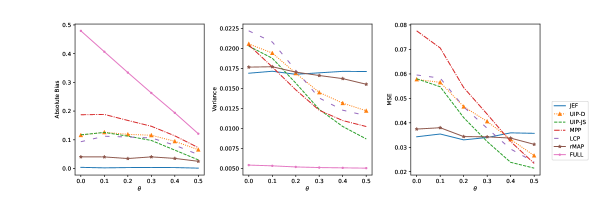
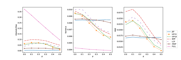
Figure 3: The absolute bias, variance and mean squared error (MSE) when varying $\theta$ from $0$ to $0.5$ under Jeffreys prior, UIP-Dirichlet, UIP-JS, MPP, LCP, rMAP and full-borrowing methods with sample size $n=60$ (top) and $n=120$ (bottom) for continuous data.

To assess the performance of different methods, we show the absolute biases, variances and MSEs in Figure 3 when varying the mean parameter of the current dataset from $0$ to $0.5$ for $n=60$ and $120$, respectively. The bias of $\theta$, defined as $\mathrm{E}\left\{(\theta-\theta_{0})|D\right\}$ where $\theta_{0}$ is the true value, measures the accuracy for the posterior distribution of $\theta$. The variance, denoted by $\mbox{Var}(\theta|D)$, measures the precision of the posterior distribution. The MSE compromises both the accuracy and precision of the posterior distribution, which is defined as $\mathrm{E}\left\{(\theta-\theta_{0})^{2}|D\right\}$. We omit the MSE curve for the full-borrowing method in order to display other MSE curves better. We replicate 1000 experiments and take the average for each metric.

All five informative priors show better performances when the historical datasets are more consistent with the current dataset. Among them, the rMAP prior yields the most robust results in terms of all three metrics. However, when the mean parameter of the current dataset is close to the counterparts of the historical datasets, its variance is only slightly smaller than that under Jefferys’ prior. It illustrates that the rMAP prior tends to be too conservative to borrow enough information in some cases. The other four informative priors have a similar trend, i.e., they all borrow information more aggressively when the historical datasets are coherent with the current one, yet sacrifice the robustness. In terms of MSE, the UIP-JS method is consistently better than the LCP and MPP methods under both small and large sample sizes. The UIP-Dirichlet method performs the best under large sample size ($n=120$) while it has comparable performance with LCP and MPP methods under small sample size ($n=60$). Larger sample size yields better estimates of the weight parameters $w_{k}$’s, which enhance the overall performance of the UIP-Dirichlet method.

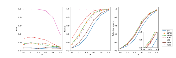
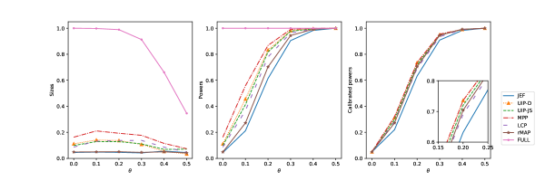
Figure 4: Results of hypothesis testing $H_{0}:\theta=\theta_{0}$ vs $H_{1}:\theta\neq\theta_{0}$ when varying the true value of the mean parameter from $0$ to $0.5$ for continuous data with sample size $n=60$ (top) and $n=120$ (bottom) under Jeffreys prior, UIP-Dirichlet, UIP-JS, MPP, LCP, rMAP and full-borrowing methods; left panels: the test size; middle panels: power; right panels: the calibrated power when controlling the size at $0.05$.

We further conduct hypothesis testing for $H_{0}:\theta=\theta_{0}$ vs $H_{1}:\theta\neq\theta_{0}$. The $95\%$ equal-tailed credible interval (CI) is used as the criterion for the hypothesis testing, i.e., if the CI does not contain $\theta_{0}$, we reject $H_{0}$. In the left column of Figure 4, we present the sizes when varying the mean parameter for the current dataset from $0$ to $0.5$ with $n=60,120$ under $1000$ repetitions. In terms of the type I error, all five informative priors are robust compared with the-full borrowing method, and the MPP method has the largest type I error among the five informative priors. The UIP methods and LCP have comparable sizes, while the results of the rMAP prior are most close to those of Jeffreys prior. We show the power in the middle column of Figure 4. The rMAP prior has the lowest power among the five informative priors as it is conservative in borrowing information from historical datasets. While yielding the largest type I error, the MPP method also has largest power. The UIP and LCP methods produce comparable results.

To make a fair comparison in power, we recalibrate the test size of $H_{0}:\theta=0$ for all seven methods to be 0.05 and present the power curves in the right column of Figure 4. For continuous data, it is impossible to control the size at $0.05$ for the full-borrowing method, which is thus omitted. After calibration, there are significant gaps between the informative priors and Jeffreys prior, revealing that all the informative priors gain information from historical datasets. The rMAP prior has the overall lowest calibrated power, which is consistent with the observation that it is conservative in borrowing information. In fact, in terms of the calibrated power, the UIP methods are consistently better than the rMAP prior. Under the small sample size ($n=60$), the UIP-JS method has the largest calibrated power, while the MPP method leads to the best performance for $n=120$.

The test sizes under the MPP, LCP and UIP methods are significantly inflated compared with that under Jeffreys prior. In fact, size inflation is common for informative priors and a similar phenomenon is observed in the simulations by Hobbs et al. (2011); Gravestock and Held (2019); Banbeta et al. (2019). When incorporating information from historical data to increase the power, it also tends to inflate the test size. To solve this issue, we can calibrate the size by enlarging the coverage probability of the credible interval. In real data application, the calibration can be implemented by resampling methods, e.g., bootstrap or permutation, to reconstruct the null distribution. In the simulation studies, all the MPP, LCP and UIP methods yield significantly larger power even after calibration of the size compared with Jeffreys prior which demonstrates that these informative priors can borrow information from the historical data. Moreover, not only are informative priors used for frequenstist hypothesis testing, but they can also help to estimate the parameter of interest. Figure 3 shows that when the historical datasets do not deviate dramatically from the current dataset, informative priors can help to decrease the MSE of the parameter estimates compared with Jeffreys prior.

5 Application

As an illustration, we apply the UIP-Dirichlet and UIP-JS methods to six phase III clinical studies to investigate the efficacy of memantine in Alzheimer’s disease (AD) (Winblad et al., 2007; Rive et al., 2013). All the six trials were double-blind and placebo-controlled. Among the six trials, only the trial MRZ-9605 (Reisberg et al., 2003) had a treatment period of $28$ weeks, while the others had a duration of $24$ weeks. Trials MEM-MD-02 (Tariot et al., 2004) and MEM-MD-12 (Porsteinsson et al., 2008) took memantine as an add-on therapy in patients who already received acetylcholinesterase inhibitors (AChEIs) and other trials assessed memantine as a monotherapy. Trials MRZ-9605, MEM-MD-01 (van Dyck et al., 2007) and MEM-MD-02 recruited patients with moderately severe to severe AD, while trials LU-99679 (Bakchine and Loft, 2008), MEM-MD-10 (Peskind et al., 2006) and MEM-MD-12 enrolled patients with mild to moderate AD. The severity of AD was defined by the scores of the mini-mental state exam (MMSE).

In our analysis, we regard MEM-MD-12 as the current study and the remaining trials as historical studies. The efficacy of the behavioral domain could be measured at the end of the trial by the change of the neuropsychiatric inventory (NPI) score from the baseline, and a decrease in the NPI score indicated clinical improvement (Cummings et al., 1994). Among the six historical trials, the results of trials LU-99679 and MEM-MD-12 appeared to be closer than others. For trials LU-99679 and MEM-MD-12, the changes in the NPI scores indicated that the efficacy of memantine was inferior to that of placebo in the behavioral domain, while the rest of the trials demonstrated the opposite results.

Specifically, we analyze the changes of the NPI scores with a linear model,

$$Y_{i}\sim N(\beta_{0}+\beta_{1}X_{i},\sigma^{2}),$$

where $Y_{i}$ is the change of the NPI score for patient $i$, $X_{i}$ is an indicator variable taking a value of $1$ if patient $i$ received memantine, and $0$ otherwise. Our goal is to determine whether memantine is superior to placebo in the behavioral domain, i.e., whether $\beta_{1}$ is significantly smaller than $0$. We fit the data of the six trials separately by classical Bayesian linear regression with noninformative priors for $\beta_{0}$, $\beta_{1}$ and $\sigma^{2}$, i.e., $\beta_{0}\sim N(0,10^{2})$, $\beta_{1}\sim N(0,10^{2})$ and $\sigma^{2}\sim\mathrm{InvGa}(0.01,0.01)$.

The results in Table 1 show that among all the six studies, MEM-MD-02 is the only trial with a statistically significant result as its upper bound of the $95\%$ equal-tailed CI for $\beta_{1}$ is below $0$. The estimates of $\beta_{1}$ in trials LU-99679 and MEM-MD-12 are positive and close to each other, and thus we expect that more information would be borrowed from LU-99679 compared with the other historical datasets.

We analyze the data from MEM-MD-12 while including the five historical datasets using the UIP-Dirichlet and UIP-JS methods, in comparison with MPP, LCP and rMAP. As our main interest focuses on the parameter $\beta_{1}$, we only impose the informative priors on $\beta_{1}$ while for the other parameters we adopt non-informative priors. To prevent the historical data from overwhelming the current data, we set $M\sim\mathrm{Uniform}(0,n)$ as the hyper-prior for the total amount parameter $M$ for the UIP methods, where $n$ is the sample size of the current trial MEM-MD-12.

As shown in Table 2, all the five informative priors demonstrate the ability of adaptively borrowing information for $\beta_{1}$ from historical data as their $95\%$ CIs of $\beta_{1}$ are narrower compared with the original CI of $\beta_{1}$ without any prior information for MEM-MD-12 in Table 1. The UIP-Dirichlet, UIP-JS and rMAP methods yield similar results in terms of $\beta_{0}$ and $\beta_{1}$ while the MPP and LCP methods are more analogous with each other. Among the five informative priors, the $95\%$ CI using the rMAP prior is the widest, as the rMAP prior is more conservative in borrowing information. Furthermore, even when we leverage the same non-informative prior for $\beta_{0}$, the $95\%$ CIs of $\beta_{0}$ under UIP and rMAP are narrower than those in Table 1, while for MPP and LCP, the estimates and $95\%$ CIs of $\beta_{0}$ are essentially unchanged compared with the original results for MEM-MD-12 in Table 1.

For the total amount parameter $M$, the UIP-Dirichlet and UIP-JS methods lead to comparable results, 137 versus 144, indicating intermediate borrowing of the historical data compared with the sample size of the current data $261$. The ESS of UIP-Dirichlet is $119$ and that of UIP-JS is $140$, which justifies the observation in Section 3.4, i.e., the ESS of UIP is comparable with the corresponding total amount parameter $M$. Nonetheless, the weight parameters of the two methods are slightly different. The weight parameters under the UIP-Dirichlet method are $(0.239,0.148,0.217,0.200,0.196)$ for the five trials LU-99679, MEM-MD-01, MEM-MD-02, MEM-MD-10 and MRZ-9605, respectively while those under the UIP-JS method are $(0.357,0.155,0.159,0.073,0.256)$. As expected, both methods assign notably larger weights to the trial LU-99679 compared with other historical datasets, while the heterogeneity of the weight parameters under UIP-JS is larger than that under UIP-Dirichlet.

In summary, under all the five informative priors, although the CIs of $\beta_{1}$ become narrower, they still cover $0$. Thus, in terms of the NPI score, the efficacy of memantine in the behavioural domain is not shown to be superior to that of placebo, which is consistent with the original conclusion in Porsteinsson et al. (2008).

The statistics of the NPI scores for both the memantine and placebo groups of the six trials are presented in the Web Table 1 of the supplementary material, which also contains more information on the numerical studies.

6 Discussion

We propose an adaptively informative prior using historical data, which is elicited from an information perspective. We demonstrate that the UIP framework has many similarities to other commonly used adaptive priors and yields comparable performances. The proposed UIP methods are easy to implement for multiple historical datasets, whose parameters have intuitive interpretations. The weight parameters $w_{k}$ can be interpreted as the relative importance of the historical datasets in comparison with each other. The amount parameter $M$ reveals the the total information contained in the prior. For both binary and continuous data, we show that the amount parameter $M$ typically has a comparable value with the prior effective sample size defined by Morita et al. (2008).

The UIP methods are useful in the clinical trial field, as it is not uncommon to find multiple related trials for any ongoing study, especially, for the control arm of clinical trials. While we mainly illustrate the UIP methods under the single-arm trial case, it is also extended to the linear model settings. In practice, it is typically not easy to obtain the patient-level historical datasets. An important feature of the UIP framework is that it does not need the patient-level historical data while some informative priors (e.g., MPP and LCP methods) need such data. For example, in a study involving a linear regression model with multiple covariates, to adopt the UIP-Dirichlet method for the parameter of interest we only need the estimate of that parameter and its corresponding confidence interval which would be commonly reported in publications of the historical study. However, as the MPP and LCP are derived from the likelihood, the complete patient-level historical data are required.

7 Supplementary Material

Web Table 1 shows the summary statistics of the NPI scores for both the memantine and placebo groups of six trials in Section 5. Web Figure 1 presents the effective sample sizes of the conditional UIP (Morita et al., 2008) and marginal UIP (Morita et al., 2012) for binary data. Web Figure 2 displays the dynamic trend of the amount parameter $M$, weight parameters $w_{k}$’s and the absolute weights $Mw_{k}$’s for binary data.

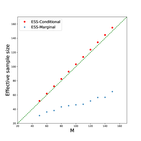
Figure 1: The effective sample size (ESS) of the the conditional UIP and that of the marginal UIP for continuous data when varying $M$ from $50$ to $150$. The dashed green line is the diagonal line.

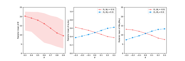
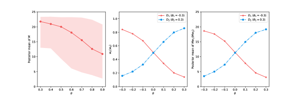
Figure 2: Under the UIP-Dirichlet (top) and UIP-JS (bottom) methods for continuous data with 100 repetitions, when the population mean of the current dataset $D$ varies from $0.3$ to $0.9$, the trend of $M$ (left panels) with the red shadow area indicating the $95\%$ confidence interval and when the population mean of the current dataset $D$ varies from $-0.3$ to $0.3$, the trends of $w_{1}$ and $w_{2}$ (middle panels) and the trends of $Mw_{1}$ and $Mw_{2}$ (right panels).

Table 1: The results of Bayesian linear regression fitted separately to each of the six trials and the corresponding weight assigned to each dataset when using UIP-Dirichlet and UIP-JS respectively.

	$\beta_{0}$		$\beta_{1}$		UIP-Dirichlet	UIP-JS
Trials	Estimate	$95\%$ CI	Estimate	$95\%$ CI	Weight	Weight
MEM-MD-12	0.865	(-1.065, 2.838)	0.093	(-2.553, 2.801)	1	1
LU-99679	-2.173	(-4.595, 0.349)	1.819	(-1.185, 4.744)	0.239	0.357
MEM-MD-01	0.479	(-2.012, 2.974)	-2.568	(-5.994, 0.950)	0.148	0.155
MEM-MD-02	2.701	(0.811, 4.650)	-3.412	(-6.094, -0.745)	0.217	0.159
MEM-MD-10	2.796	(0.233, 5.318)	-2.017	(-5.595, 1.725)	0.200	0.073
MRZ-9605	2.704	(-0.541, 6.045)	-2.541	(-7.058, 1.968)	0.196	0.256
CI: credible interval.

Table 2: The results using the UIP-Dirichlet, UIP-JS, MPP, LCP and rMAP methods for the current study MEM-MD-12 by borrowing information from five historical trials LU-99679, MEM-MD-01, MEM-MD-02, MEM-MD-10 and MRZ-9605.

Parameters		UIP-Dirichlet	UIP-JS	MPP	LCP	rMAP
$\beta_{0}$	Estimate	1.232	1.128	0.856	0.849	1.166
	$95\%$ CI	(-0.560, 2.974)	(-0.571, 2.851)	(-1.127, 2.809)	(-1.104, 2.780)	(-0.705, 2.942)
$\beta_{1}$	Estimate	-0.626	-0.400	-0.837	-0.746	-0.476
	$95\%$ CI	(-2.783, 1.643)	(-2.350, 1.639)	(-3.132, 1.502)	(-3.061, 1.639)	(-2.740, 2.020)

References

- Bakchine and Loft (2008) Bakchine, S. and Loft, H. (2008). Memantine treatment in patients with mild to moderate alzheimer’s disease: results of a randomised, double-blind, placebo-controlled 6-month study. Journal of Alzheimer’s Disease, 13(1):97–107.
- Banbeta et al. (2019) Banbeta, A., van Rosmalen, J., Dejardin, D., and Lesaffre, E. (2019). Modified power prior with multiple historical trials for binary endpoints. Statistics in medicine, 38(7):1147–1169.
- Borghaei et al. (2015) Borghaei, H., Paz-Ares, L., Horn, L., Spigel, D. R., Steins, M., Ready, N. E., Chow, L. Q., Vokes, E. E., Felip, E., Holgado, E., et al. (2015). Nivolumab versus docetaxel in advanced nonsquamous non–small-cell lung cancer. New England Journal of Medicine, 373(17):1627–1639.
- Brahmer et al. (2015) Brahmer, J., Reckamp, K. L., Baas, P., Crinò, L., Eberhardt, W. E., Poddubskaya, E., Antonia, S., Pluzanski, A., Vokes, E. E., Holgado, E., et al. (2015). Nivolumab versus docetaxel in advanced squamous-cell non–small-cell lung cancer. New England Journal of Medicine, 373(2):123–135.
- Cummings et al. (1994) Cummings, J. L., Mega, M., Gray, K., Rosenberg-Thompson, S., Carusi, D. A., and Gornbein, J. (1994). The neuropsychiatric inventory: comprehensive assessment of psychopathology in dementia. Neurology, 44(12):2308–2308.
- Duan et al. (2006) Duan, Y., Ye, K., and Smith, E. P. (2006). Evaluating water quality using power priors to incorporate historical information. Environmetrics: The Official Journal of the International Environmetrics Society, 17(1):95–106.
- Goodfellow et al. (2014) Goodfellow, I., Pouget-Abadie, J., Mirza, M., Xu, B., Warde-Farley, D., Ozair, S., Courville, A., and Bengio, Y. (2014). Generative adversarial nets. In Advances in neural information processing systems, pages 2672–2680.
- Gravestock and Held (2019) Gravestock, I. and Held, L. (2019). Power priors based on multiple historical studies for binary outcomes. Biometrical Journal, 61(5):1201–1218.
- Hobbs et al. (2011) Hobbs, B. P., Carlin, B. P., Mandrekar, S. J., and Sargent, D. J. (2011). Hierarchical commensurate and power prior models for adaptive incorporation of historical information in clinical trials. Biometrics, 67(3):1047–1056.
- Hunter (2014) Hunter, D. R. (2014). Notes for a graduate-level course in asymptotics for statisticians. Penn State University, Pennsylvania.
- Ibrahim et al. (2000) Ibrahim, J. G., Chen, M.-H., et al. (2000). Power prior distributions for regression models. Statistical Science, 15(1):46–60.
- Itzkovitz et al. (2010) Itzkovitz, S., Hodis, E., and Segal, E. (2010). Overlapping codes within protein-coding sequences. Genome research, 20(11):1582–1589.