Super exponential divergence of periodic points for $C^{1}$-generic partially hyperbolic homoclinic classes

Abstract

A diffeomorphism $f$ is called super exponential divergent if for every $r>1$, the lower limit of $\#\mbox{Per}_{n}(f)/r^{n}$ diverges to infinity as $n$ tends to infinity, where $\mbox{Per}_{n}(f)$ is the set of all periodic points of $f$ with period $n$. This property is stronger than the usual super exponential growth of the number of periodic points. We show that for a three dimensional manifold $M$, there exists an open subset $\mathcal{O}$ of $\mbox{Diff}^{1}(M)$ such that diffeomorphisms with super exponential divergent property form a dense subset of $\mathcal{O}$ in the $C^{1}$-topology. A relevant result of non super exponential divergence for diffeomorphisms in a locally generic subset of $\mbox{Diff}^{r}(M)\ (1\leq r\leq\infty)$ is also shown.

2020 Mathematics Subject Classification: 37C20, 37C25, 37C29, 37D30

Key words and phrases: non-uniform hyperbolicity, partial hyperbolicity, heterodimensional cycle super exponential growth, number of periodic points.

1 Introduction

1.1 Backgrounds

The investigation of the growth of the number of periodic points for dynamical systems is a fundamental problem. For uniformly hyperbolic systems, we know that the growth of the number of periodic points cannot be faster than some exponential functions. Then a natural question is that what happens for systems which fail to be uniformly hyperbolic in a robust fashion.

A fundamental result is given by Artin and Mazur, which asserts that for a dense subset of $C^{r}$ maps of a compact manifold into itself with the uniform $C^{r}$ topology, the number of isolated periodic points grows at most exponentially [AM]. Meanwhile, there are some results for locally generic maps. For instance, Bonatti, Díaz and Fisher shows that generically in $\mbox{Diff}^{1}(M)$, if a homoclinic class contains periodic points of different indices, then it exhibits super exponential growth of number of periodic points [BDF]; For certain semi-group actions on the interval, Asaoka, Shinohara and Turaev construct $C^{r}$ $(r\geq 1)$ open set in which $C^{r}$ generic maps exhibit super exponential growth of number of periodic points [AST]; For $C^{r}$ diffeomorphisms of compact smooth manifolds, they also construct local $C^{r}$ generic subset with fast growth of number of periodic points under certain conditions about the signatures of non-linearities and Schwarzian derivatives of the transition maps [AST2]; Berger shows that for $2\leq r\leq\infty$ and manifolds of dimension greater than 1, there exists open set $\mathcal{O}\subset\mbox{Diff}^{r}(M)$ in which $C^{r}$ generic $f$ displays a fast growth of the number of periodic points [Be]. Thus one may consider the difference of the growth as a probe of the degree of the non-hyperbolicity which the system exhibits.

Let us be more precise. Given a set $X$ and a map $f:X\to X$, we say that $x\in X$ is a periodic point of period $n$ (where $n\geq 1$) if $f^{n}(x)=x$ and $n$ is the least positive integer for which this equality holds. In particular, $x$ is called a fixed point of $f(x)=x$. We denote the set of periodic points of period $n$ of $f$ by $\mathrm{Per}_{n}(f)$.

For the investigation of the number of periodic points, we mainly focus on the ratio of $\#\mathrm{Per}_{n}(f)$ to $r^{n}\ (r>1)$. We customarily consider upper limit ($\limsup$) of the ratio when $n$ goes to infinity. $f$ is called super-exponential if for every $r>1$ the sequence $r^{-n}\#\mathrm{Per}_{n}(f)$ has upper limit equals to $+\infty$. One motivation of this definition is that the “rate of exponential growth” of the number of periodic points comes from the investigation of the convergence radius of dynamical zeta function. The positivity of the convergence radius is equivalent to the finitude of the upper limit of the ratio. In this case, at least a subsequence of $\#\mbox{Per}_{n}(f)$ grows exponentially fast, which implies that the dynamics exhibits relatively complicated behaviour. On the other hand, the cases of super exponentially fast growth also appear very often, as aforementioned papers indicated.

Meanwhile, as a measure of non-uniform hyperbolicity it is interesting to ask what happens for the lower limit ($\liminf$) of the ratio. Indeed, the lower limit provides us more information about the number of $n$-periodic points for every sufficiently large $n$. It is not easy to construct an diffeomorphism around which, maps whose lower limit of the ratio divergent to $+\infty$ exist persistently (for instance, in a dense or residual subset of a neighbourhood of the initial diffeomorphism). In this paper, we provide such an example.

We say that $f$ is super-exponentially divergent if for every $r>1$ the sequence $r^{-n}\#\mathrm{Per}_{n}(f)$ has lower limit equals to $+\infty$. Indeed, this is equivalent to say that the limit exists and it is equal to $+\infty$. Let $\mbox{Diff}^{1}(M)$ denote the space of $C^{1}$ diffeomorphisms of a manifold $M$, endowed with the $C^{1}$ topology.

Theorem 1.

There exists a three dimensional closed manifold $M$ such that the following holds: There exist an non-empty open set $\mathcal{O}\subset\mathrm{Diff}^{1}(M)$ and a dense subset $\mathcal{D}$ of $\mathcal{O}$ such that every diffeomorphism in $\mathcal{D}$ is super-exponentially divergent.

Let us make some comments. Our construction is based on the bifurcation of heterodimensional cycles. Since heterodimensional cycles exist only for manifolds whose dimension is greater than two, we are not sure a similar result holds for surface diffeomorphisms. We gave this result for $C^{1}$-regularity. As we will see, our technique heavily depends on the nature of $C^{1}$-distance. Thus the $C^{r}$-case for $r>1$ is open.

In the following, we give the description of the open set $\mathcal{O}$.

1.2 Results

Let $M$ be a closed $n$-dimentional Riemannian manifold. We fix a Riemaniann metric $\|\cdot\|$ on $TM$ and a metric $d$ on $M$. Denote by $\mathrm{Diff}^{1}(M)$ the space of $C^{1}$ diffeomorphisms of $M$ endowed with the $C^{1}$ topology. We also fix a metric $\mathrm{dist}(f,g)$ for every pair of $f,g\in\mathrm{Diff}^{1}(M)$ which is compatible with the $C^{1}$ topology.

Let us recall some notion for non-uniformly hyperbolic systems, following [BDU]. For further information, see for instance [BDV]. Let $f\in\mathrm{Diff}^{1}(M)$ and $\Lambda\subset M$ be an $f$-invariant set, that is, $f(\Lambda)=\Lambda$ holds. Let $E,F$ be subbundles of $TM|_{\Lambda}$ which are invariant under $Df$ respectively. $E_{x}\cap F_{x}=\{0\}$ for every $x\in\Lambda$. We say that $E\oplus F$ is a dominated splitting if there exists a positive real number $\alpha$ strictly smaller than 1 such that for every $x\in\Lambda$ we have $\|Df|_{E_{x}}\|\cdot\|Df^{-1}|_{F_{f(x)}}\|<\alpha$, where $\|Df|_{E_{x}}\|$ denotes the operator norm of $Df|_{E_{x}}$ with respect to the Riemannian metric.

We say that $\Lambda$ is strongly partially hyperbolic if there is a splitting $TM|_{\Lambda}=E^{s}\oplus E^{c}\oplus E^{u}$ such that $E^{s}\oplus(E^{c}\oplus E^{u})$ and $(E^{s}\oplus E^{c})\oplus E^{u}$ are dominated splittings with $\dim E^{c}=1,\dim E^{s}\geq 1$ and $\dim E^{u}\geq 1$, $E^{s}$ is uniformly contracting and $E^{u}$ is uniformly expanding. We say that $Df$ is orientation preserving if if $E^{s},E^{c},E^{u}$ are all orientable and $Df$ preserves these orientations.

Suppose we have a pair of hyperbolic periodic points $P_{1},P_{2}\in\Lambda$. We say that they are adapted if $\mathrm{u}\mbox{-}\mathrm{ind}(P_{1})=\dim(E^{u})+1$ and $\mathrm{u}\mbox{-}\mathrm{ind}(P_{2})=\dim(E^{u})$, where $\mathrm{u}\mbox{-}\mathrm{ind}(P)$ denotes the dimension of the unstable subspace of a hyperbolic periodic point $P$.

We say that $f$ is transitive (on $M$) if there is an orbit which is dense in $M$, that is, if there exists $x\in M$ such that $\{f^{n}(x)\}_{n\in\mathbb{Z}}$ is dense in $M$. A diffeomorphism $f$ is $C^{r}$-robustly transitive if there is an open neighbourhood $\mathcal{U}$ of $f$ in $\mathrm{Diff}^{r}(M)$ equipped with the $C^{r}$ topology such that every $g\in\mathcal{U}$ is transitive.

The following is our first result.

Theorem 2.

Let $M$ be a three dimensional closed manifold and $f$ be a $C^{1}$-robustly transitive diffeomoprhism for which the entire manifold $M$ is a strongly partially hyperbolic set. Suppose that $f$ has two hyperbolic fixed points $P_{1}$ and $P_{2}$ having $u$-indices $2$ and $1$ respectively and $Df$ preserves the orientations of the strongly partially hyperbolic splitting over $M$. Then there exist a $C^{1}$-neighbourhood $\mathcal{U}$ of $f$ in $\mathrm{Diff}^{1}(M)$ and a dense subset $\mathcal{D}$ of $\mathcal{U}$ satisfying the following: Every $g\in\mathcal{D}$ is super-exponentially divergent.

Theorem 2 is a consequences of general perturbation results together with the following analytic result.

First, let us state the analytic result.

Theorem 3.

Let $M$ be a three dimensional closed manifold. Suppose $f$ satisfies the following:

• (Codimension-1 property) There are hyperbolic fixed points $P_{1}$ and $P_{2}$ of $f$ with $\mathrm{u}\mbox{-}\mathrm{ind}(P_{1})=2$ and $\mathrm{u}\mbox{-}\mathrm{ind}(P_{2})=1$.

• (Simplicity property) The weakest unstable eigenvalue of $P_{1}$ and the weakest stable eigenvalue of $P_{2}$ are both real, positive and have multiplicity one.

• (Existence of a strong heteroclinic intersection) Let $W^{ss}(P_{2})$ denote the stong stable manifold of $P_{2}$ corresponding to the strong stable eigenvalue of $Df(P_{2})$. Then $W^{u}(P_{1})\cap W^{ss}(P_{2})\neq\emptyset$.

• (Existence of a quasi-transverse intersection) $W^{u}(P_{2})\cap W^{s}(P_{1})\neq\emptyset$.

Then, there is a diffeomorphism $g$ which is arbitrarily $C^{1}$ close to $f$ such that for every $r>1$ we have

$$\lim\limits_{n\to\infty}\dfrac{\#\mathrm{Per}_{n}(g)}{r^{n}}=+\infty.$$

Notice that this implies $\liminf_{n\to\infty}\dfrac{\#\mathrm{Per}_{n}(g)}{r^{n}}=+\infty$.

One important condition in the assumptions of Theorem 3 is that we assume $P_{1},P_{2}$ are fixed points of $f$. In this article, we are interested in the behavior of lower limit of the number of periodic points. In many situations, the difference whether the periodic orbit we are interested in has non-trivial period or not can be overcome by taking power of the dynamics. On the other hand, as we will see later, this strategy does not work in a simple way for the investigation of the lower limit. The investigation of to what extent we can relax this fixed point assumption would be an interesting topic, but we will not pursue this problem in this paper.

The following perturbation result tells us that for systems which satisfy the hypothesis of Theorem 2, we can obtain the assumptions of Theorem 3 up to an arbitrarily small $C^{1}$ perturbation.

Proposition 1.1.

Let $f$ be a $C^{1}$-robustly transitive diffeomorphism on a smooth compact three dimensional manifold such that the entire manifold is strongly partially hyperbolic. Assume that there are two hyperbolic fixed points $P_{1}$ and $P_{2}$ whose indices are $2$ and $1$ respectively and $Df$ preserves the orientation. Then, there exists $g\in\mathrm{Diff}^{1}(M)$ arbitrarily $C^{1}$ close to $f$ such that $g$ satisfies the hypotheses (T1-4) of Theorem 3.

The proof of Proposition 1.1 will be given in Section 3.

Let us give a “local version” of Theorem 2. In Theorem 2, we stated the result under the condition that the diffeomorphism is robustly transitive. While this condition is easy to understand, it is not the essential one which we need to reach the conclusion. Below we give Theorem 4, in which the assumption for the super exponential divergence is stated in terms of homoclinic classes and this statement makes it easier to grasp about the mechanism of the result.

Let us recall the notion of homoclinic classes. A homoclinic class of a hyperbolic periodic saddle $P$ of a diffeomorphism $f$, denoted by $H(P;f)$ or $H(P)$, is defined to be the closure of transversal intersections of the stable and unstable manifolds of $P$. We can equivalently define $H(P)$ as the closure of all hyperbolic periodic saddles $Q$ homoclinically related to $P$ (i.e. the stable manifold of $P$ transversally intersects the unstable manifolds of $Q$ and vice versa). Homoclinic classes are always invariant and transitive, but not necessarily hyperbolic in general (see for instance [ABCDW]).

Theorem 4.

Let $M$ be a three dimensional closed manifold. Suppose $f\in\mathrm{Diff}^{1}(M)$ satisfies the following:

• There are hyperbolic fixed points $P_{1}$ and $P_{2}$ of $f$ contained in the same homoclinic class $H(P_{1})$ with $\mathrm{u}\mbox{-}\mathrm{ind}(P_{1})=2$ and $\mathrm{u}\mbox{-}\mathrm{ind}(P_{2})=1$;

• The weakest unstable eigenvalue of $P_{1}$ and the weakest stable eigenvalue of $P_{2}$ are both real, positive and have multiplicity one;

• $W^{u}(P_{1})$ intersects $W^{ss}(P_{2})$ transversally.

Then, there exists an arbitrarily small $C^{1}$-perturbation $g$ of $f$ such that $g$ is super exponential divergent.

The proof of Theorem 4 will be given in Section 3.

Let us see the strategy of the proof of Theorem 3. Given a heterodimensional cycle associated to two hyperbolic fixed points $P_{1}$ and $P_{2}$ of $f$, in other words, $P_{1}$ and $P_{2}$ are index adapted with $W^{u}(P_{1})\cap W^{s}(P_{2})\not=\emptyset$ and $W^{u}(P_{2})\cap W^{s}(P_{1})\not=\emptyset$. Following the argument in [BD], we linearize the dynamics around $P_{1}$ and $P_{2}$. We also make the transition map along the heteroclinic points $Q_{1}$ and $Q_{2}$ affine, which are compatible with the linear maps around $P_{1}$ and $P_{2}$. These dynamics are called a simple cycle. A direct calculation shows that we can find a sequence of periodic points with weak center Lyapunov exponents. Thus, by exploiting the flexibility of the $C^{1}$-topology, we can increase the number of periodic points as much as we want by perturbing in the center direction.

This is the strategy of the proof of [BDF]. In our problem, we furthermore need to investigate the frequency of the period of the weak periodic points. To be more precise, we need to confirm the occurrence of periods of weak periodic points for every sufficiently large integer. By investigating the above calculation carefully, we can observe that, under certain quantitative assumption on the characteristics of the simple cycle, the periods exhaust all sufficiently large integers eventually by an arbitrarily small $C^{1}$ perturbation. In our proof, an additional hypothesis on the simple cycle is needed. We call our simple cycle as SH-simple cycle (where SH stands for “Strongly Heteroclinic”), meaning that in addition, the unstable manifold of $P_{1}$ intersects the strong stable manifold of $P_{2}$.

A natural question regarding Theorem 1 is if one could replace “dense” to some stronger condition such as residual or open and dense. For instance, one might wonder the following:

Question 1.

Does there exist an open subset $\mathcal{U}$ of $\mbox{Diff}^{1}(M)$ such that generically in $\mathcal{U}$, diffeomorphisms are super exponential divergent?

While we do not have an answer, in Section 6 we will prove one result about the lower limit of the number of periodic points valid for diffeomorphisms in a residual subset of $\mbox{Diff}^{r}(M)$ where $1\leq r\leq\infty$, based on the argument of Kaloshin [Ka].

Theorem 5.

Given $1\leq s\leq+\infty$ and a super-exponential sequence $(a_{n})$, there exists an residual set $\mathcal{R}$ of $\mathrm{Diff}^{s}(M)$ such that the following holds: for every $f\in\mathcal{R}$, we have $\liminf_{n\to\infty}\#\mathrm{Per}_{n}(f)/a_{n}\to 0$.

Thus we cannot extend Theorem 1 in a straightforward way and this shows the significance of Theorem 1. Notice that Theorem 5 does not answer Question 1, because there is no “slowest” super exponentially increasing sequence.

This paper will be organized as follows. In Section 2, after giving some basic definitions and notations on SH-simple cycles, we provide the proof of Theorem 3 by assuming several results which will be proved in the following sections. In Section 3, we will discuss the proof of Theorem 4 and how to prove Theorem 2 from Theorem 3. Section 4 is devoted to the proof of Proposition 2.5, a perturbation result for obtaining SH-simple cycles. In Section 5, we prove Proposition 2.6, an analytic result for SH-simple cycles is shown. In Section 6, by using a theorem of [Ka], we prove Theorem 5, a generic result of super exponential divergence with respect to a given speed.

Acknowledgements.    This paper has been supported by the the JSPS KAKENHI Grant Number 18K03357. XL is supported by the Youth Program of National Natural Science Foundation of China (11701199) and the Fundamental Research Funds for the Central Universities, HUST: 2017 KFYXJJ095. KS thank the warm hospitality of Huazhong University of Science and Technology. We thank Masayuki Asaoka and Ken-ichiro Yamamoto for their suggestions and comments.

2 Preliminaries and Strategies

In this section, we prepare some definitions and cite known results which are used throughout this paper.

Then, we state some propositions which will be used for the proof of Theorem 3. Finally, assuming these propositions we give the proof of Theorem 3.

2.1 SH-simple cycles

Let us give the definition of simple cycles. In this paper, it is more convenient if we define a wider class of simple cycles, which we call SH-simple cycles. Let us give the definition of it.

Let $\mathbb{D}_{r}^{n}:=\{x\in\mathbb{R}^{n}\mid\|x\|<r\}$, where $\|\cdot\|$ denotes the Euclidian norm and $r$ is some positive real number. Let $d_{s},d_{c},d_{u}$ be positive integers and put $d=d_{s}+d_{c}+d_{u}$ and $\mathbf{d}=(d_{s},d_{c},d_{u})$. A subset $\mathbb{D}^{\mathbf{d}}=\mathbb{D}_{r_{s}}^{d_{s}}\times\mathbb{D}_{r_{c}}^{d_{c}}\times\mathbb{D}_{r_{u}}^{d_{u}}$ of $\mathbb{R}^{d}$ is called a polydisc of $\mathbb{R}^{d}$ of index $\mathbf{d}$. We call the numbers $\mathbf{d}$ and $(r_{s},r_{c},r_{u})$ the index and the size of the polydisc $\mathbb{D}^{\mathbf{d}}$ respectively. In the following, we only consider the case $d_{c}=1$. Thus we have $\mathbf{d}=(d_{s},1,d_{u})$.

We first prepare two definitions, which describe the local dynamics around the fixed point and the transition dynamics near the heteroclinic point of SH-cycles respectively.

Definition 2.1.

Let $f\in\mathrm{Diff}^{1}(M)$ and $P$ be its fixed point. We say that a coordinate neighbourhood $(U,\phi)$ around $P$ is an linearized neighbourhood of index $\mathbf{d}$ if the followings hold:

• $\phi(U)\subset\mathbb{R}^{\mathbf{d}}$ is a polydisc of index $\mathbf{d}$, that is, $\phi(U)=\mathbb{D}_{r_{s}}^{d_{s}}\times\mathbb{D}_{r_{c}}^{1}\times\mathbb{D}_{r_{u}}^{d_{u}}$ for some size $(r_{s},r_{c},r_{u})$.

• There exist a contracting linear map $\Lambda:\mathbb{R}^{d_{s}}\to\mathbb{R}^{d_{s}}$, a linear map $t:\mathbb{R}\to\mathbb{R}$ and an expanding linear map $M:\mathbb{R}^{d_{u}}\to\mathbb{R}^{d_{u}}$ such that the following holds: For every $x\in U$, if $\phi(x)=(x_{s},x_{c},x_{u})$ satisfies $t(x_{c})\in\mathbb{D}_{r_{c}}^{1}$ and $M(x_{u})\in\mathbb{D}_{r_{u}}^{d_{u}}$, then we have

  $$\phi(f(x))=(\Lambda(x_{s}),t(x_{c}),M(x_{u})).$$

  We call the linear map $(x_{s},x_{c},x_{u})\mapsto(\Lambda(x_{s}),t(x_{c}),M(x_{u}))$ the linearization of $f$ near $P$. We also call the set of the points $x$ satisfying $t(x_{c})\in\mathbb{D}_{r_{c}}^{1}$ and $M(x_{u})\in\mathbb{D}_{r_{u}}^{d_{u}}$ the linearized region.

Definition 2.2.

Let $f\in\mathrm{Diff}^{1}(M)$, $P_{1}$ and $P_{2}$ be its adapted hyperbolic fixed points. Suppose that $P_{i}$ have linearized coordinate neighbourhoods $(\phi_{i},U_{i})$ for $i=1$ and $2$ with linearization $(x_{s},x_{c},x_{u})\mapsto(\Lambda_{i}(x_{s}),t_{i}(x_{c}),M_{i}(x_{u}))$ and assume that there exists a point $Q\in W^{u}(P_{1})\cap W^{s}(P_{2})\cap U_{1}$. Let $\sigma>0$ be the least positive integer such that $f^{\sigma}(Q)\in U_{2}$ holds. We say that $Q$ is an adapted transition point with respect to $(U_{1},\phi_{1})$ and $(U_{2},\phi_{2})$ if there exist positive real numbers $\kappa_{s},\kappa_{c}$ and $\kappa_{u}$ such that the followings hold:

• There exists a neighbourhood $K\subset U_{1}$ of $Q$ such that $\phi_{1}(K)$ has the form $\phi_{1}(Q)+\mathbb{D}_{\kappa_{s}}^{d_{s}}\times\mathbb{D}_{\kappa_{c}}^{1}\times\mathbb{D}_{\kappa_{u}}^{d_{u}}$, that is, $\phi_{1}(K)$ is a polydisc centered at $\phi(Q)$ of size $(\kappa_{s},\kappa_{c},\kappa_{u})$.

• Furthermore, $f^{i}(K)\cap(U_{1}\cup U_{2})=\emptyset$ for every $i=1,\ldots,\sigma-1$ and $f^{\sigma}(K)\subset U_{2}$.

• There exist three linear maps $\tilde{\Lambda}:\mathbb{R}^{d_{s}}\to\mathbb{R}^{d_{s}}$, $\tilde{t}:\mathbb{R}\to\mathbb{R}$ and $\tilde{M}:\mathbb{R}^{d_{u}}\to\mathbb{R}^{d_{u}}$ such that the following holds: For every $(X,Y,Z)\in\mathbb{R}^{\mathbf{d}}$ such that $\phi_{1}(Q)+(X,Y,Z)\in\phi_{1}(K)$ holds, we have

  $$\phi_{2}\circ f^{\sigma}\circ\phi_{1}^{-1}(\phi_{1}(Q)+(X,Y,Z))=\phi_{2}(f^{\sigma}(Q))+(\tilde{\Lambda}(X),\tilde{t}(Y),\tilde{M}(Z)).$$

We call $\tilde{t}$ the center multiplier of the transition map $f^{\sigma}$ and $K$ the transition region.

Given two hyperbolic fixed points $P_{1}$ and $P_{2}$ of different indices, we say that they form a heterodimensional cycle if the stable manifold of $P_{1}$ intersects the unstable manifold of $P_{2}$ and vice versa. Heterodimensional cycles are realized as one of the typical mechanisms which causes the non-hyperbolicity of the dynamics.

Now we are ready to state the definition of SH-simple cycles.

Definition 2.3.

Let $f\in\mathrm{Diff}^{1}(M)$. Suppose there is a heterodimensional cycle associated to $P_{1}$, $P_{2}$ and heteroclinic points $Q_{1}\in W^{u}(P_{1})\cap W^{s}(P_{2})$ and $Q_{2}\in W^{u}(P_{2})\cap W^{s}(P_{1})$. We say that the heterodimensional cycle is SH-simple if the followings hold (see Figure. 1):

• There are linearized coordinates $(U_{i},\phi_{i})$ around $P_{i}$ for $i=1,2$.

• $Q_{i}\in U_{i}$ and they are adapted heteroclinic points associated to $(U_{i},\phi_{i})$ and $(U_{i+1},\phi_{i+1})$ with transition maps $f^{\sigma_{i}}$ for $i=1,2$, where we set $(U_{3},\phi_{3})=(U_{1},\phi_{1})$.

• The $\mathbb{R}^{d_{u}}$-coordinate of $\phi_{1}(Q_{1})$ is $\boldsymbol{0}^{d_{u}}$.

• The $\mathbb{R}^{d_{c}}$-coordinate of $\phi_{2}(f^{\sigma_{1}}(Q_{1}))$ is $0$.

• The center multipliers of the transition maps $f^{\sigma_{i}}\ (i=1,2)$ equal to 1.

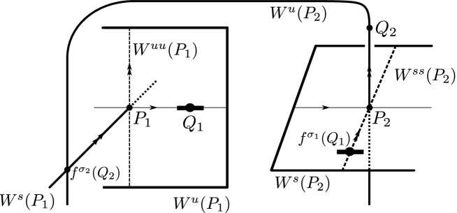
Figure 1: An illustration of an SH-simple cycle.

Remark 2.4.

Let $f$ be a diffeomorphism having a SH-simple cycle. According to the coordinates of $Q_{1}$ and $Q_{2}$, we may assume that they have the following forms:

$$\phi_{1}(Q_{1}) =(\boldsymbol{0}^{d_{s}},q_{1},\boldsymbol{0}^{d_{u}}), \phi_{2}(f^{\sigma_{1}}(Q_{1})) =(\boldsymbol{q}^{\prime}_{1},0,\boldsymbol{0}^{d_{u}}).$$

$$\phi_{2}(Q_{2}) =(\boldsymbol{0}^{d_{s}},0,\boldsymbol{q}_{2}), \phi_{1}(f^{\sigma_{2}}(Q_{2})) =(\boldsymbol{q}_{2}^{\prime},0,\boldsymbol{0}^{d_{u}}).$$

2.2 Main perturbation result

In [BD], it was proven that given a diffeomorphism having a heterodimensional cycle, by adding an arbitrarily small $C^{1}$-perturbation one can obtain another diffeomorphism such that the continuation of the heterodimensional cycle is simple, that is, the local dynamics around it is given by locally affine maps.

One of the main step of the proof of our theorem is that one can obtain similar affine dynamics from strongly heteroclinic cycles.

Proposition 2.5.

Let $f\in\mathrm{Diff}^{1}(M)$ which has two hyperbolic fixed points $P_{1}$, $P_{2}$ and satisfies all the assumptions (T1-4) in Theorem 3. Then, there exists $g\in\mathrm{Diff}^{1}(M)$ arbitrarily $C^{1}$-close to $f$ such that the continuations of $P_{1}$ and $P_{2}$ form a SH-simple cycle for $g$.

The proof of Proposition 2.5 is given in Section 4.

2.3 Main analytic result

Let us state the main analytic result about the existence of the periodic points. We prepare one definition. For a hyperbolic periodic point $P$ with index $\mathbf{d}$, its center Lyapunov exponent, denoted by $\lambda_{c}(P)$, is the real number given as follows:

$$\lambda_{c}(P):=\frac{1}{\pi}\log\|Df^{\pi}|_{E^{c}(P)}\|,$$

where $\pi$ denotes the period of $P$ and $E^{c}(P)$ denotes the center direction at $P$. It is easy to see that periodic points in the same orbit shares the same Lyapunov exponents, thus sometimes we also say Lyapunov exponents of some orbit. Usually, the notion of Lyapunov exponents are defined for invariant measures. Notice that this definition coincides with the usual one if we consider the uniformly distributed Dirac measure along the orbit of $P$. Below, for a diffeomorphisms $f\in\mathrm{Diff}^{1}(M)$ and a point $x\in M$, we put $\mathrm{orb}(P):=\{f^{i}(x)\mid i\in\mathbb{Z}\}$.

Proposition 2.6.

Let $f\in\mathrm{Diff}^{1}(M)$ with a heterodimensional cycle associated to hyperbolic fixed points $P_{1}$ and $P_{2}$. Suppose that they form a SH-simple heterodimensional cycle with respect to the coordinates $(U_{i},\phi_{i})$. Then, there exists an integer $\tilde{l}$ such that the following holds:

• For every $j\geq\tilde{l}$, there exists a periodic point $R_{j}$ of period $j$ and whose orbit admits a strongly partially hyperbolic splitting of index $\mathbf{d}$ such that the angles between $E^{s}(R_{j}),E^{c}(R_{j})$ and $E^{u}(R_{j})$ are bounded from below by some positive uniform constant independent of $j$.

• Let $\lambda_{c}(R_{j})$ be the center Lyapunov exponent of $R_{j}$. Then we have $\lambda_{c}(R_{j})\to 0$ as $j\to\infty$.

• For every $j\geq\tilde{l}$, the sequence of the orbits $\{\mathrm{orb}(R_{k})\}_{k>j}$ does not accumulate to $\mathrm{orb}(R_{j})$. In other words, for every $j\geq\tilde{l}$, there exists a neighbourhood $V_{j}$ of $\mathrm{orb}(R_{j})$ such that $V_{j}\cap\mathrm{orb}(R_{k})=\emptyset$ for every $k>j$.

2.4 Proof of Theorem 3

Using Proposition 2.5 and Proposition 2.6, let us complete the proof of Theorem 3. For the proof, we prepare a lemma. This is used to perturb a periodic point having small Lyapunov exponent into one with zero Lyapunov exponent. Notice that the availability of this lemma heavily depends on the flexibility of the $C^{1}$ topology.

Lemma 2.7 (Franks’ Lemma, see Appendix A of [BDV]).

Let $f\in\mathrm{Diff}^{1}(M)$, $\varepsilon>0$ and $P$ be a hyperbolic periodic point of period $\pi$. Let $\{G_{i}:T_{f^{i}(P)}M\to T_{f^{i+1}(P)}M\}_{i=0,\ldots,\pi-1}$ be a sequence of linear maps such that $\|Df_{f^{i}(P)}-G_{i}\|<\varepsilon$ holds for every $i$. Then, given a neighbourhood $V$ of $\mathrm{orb}(P)$, there exists $g\in\mathrm{Diff}^{1}(M)$ such that the following holds:

• $\mathrm{dist}(f,g)<\varepsilon$;

• $g(x)=f(x)$ for every $x\in M\setminus V$;

• $g$ preserves the orbit of $P$, that is, for every $i$ we have $g^{i}(P)=f^{i}(P)$;

• $Dg_{g^{i}(P)}=G_{i}$.

Now, let us complete the proof.

Proof of Theorem 3.

Let $f\in\mathrm{Diff}^{1}(M)$ having a strongly partially hyperbolic heterodimensional cycles associated to $P_{1}$ and $P_{2}$ satisfying the assumptions (T1-4) of Theorem 3. Fix an arbitrarily small $\varepsilon_{\ast}>0$.

Let us apply Proposition 2.5 to this heterodimensional cycle. Then we obtain a diffeomorphim $f_{1}$ with a SH-simple heterodimensional cycle associated to the hyperbolic continuations of $P_{1}$ and $P_{2}$ for $f_{1}$. Notice that $f_{1}$ can be chosen arbitrarily $C^{1}$-close to $f$, in particular, $\varepsilon_{\ast}/3$-close to $f$ in the $C^{1}$-distance.

Now we can apply Proposition 2.6: For $f_{1}$ we know that there exist $\tilde{l}\in\mathbb{N}$ and a sequence of periodic orbits $\{R_{j}\}_{j\geq\tilde{l}}$ satisfying the conclusion of Proposition 2.6. For each $j\geq\tilde{l}$, we take a neighbourhood $V_{j}$ of $\mathrm{orb}(R_{j})$ in such a way that $V_{j}\cap V_{j^{\prime}}=\emptyset$ holds for $j\neq j^{\prime}$.

Since $\mathrm{orb}(R_{j})$ admits a partially hyperbolic splitting and $\lambda_{c}(R_{j})\to 0$ as $j\to\infty$, there exists $L>\tilde{l}$ such that for every $j\geq L$, we can find an $\varepsilon_{\ast}/3$ $C^{1}$-small perturbation whose the support is contained in $V_{j}$ such that it preserves the orbit of $R_{j}$ and the resulted Lyapunov exponent of $R_{j}$ is equal to zero. Furthermore, we can assume that the the perturbations are arbitrarily small as $j\to\infty$.

Let us state this more precisely. For every $j\geq L$, using Franks’ Lemma we take a $C^{1}$ diffeomorphism $\rho_{j}\in\mathrm{Diff}^{1}(M)$ such that the following holds:

• $\mathrm{supp}(\rho_{j})\subset V_{j}$ where we put $\mathrm{supp}(\rho_{j}):=\{x\in M\mid\rho_{j}(x)\neq x\}$;

• For every $k\geq 0$, $(\rho_{j}\circ f_{1})^{k}(R_{j})=f_{1}^{k}(R_{j})$. In particular, $R_{j}$ is still a periodic point of period $j$ for $\rho_{j}\circ f_{1}$.

• $\lambda_{c}(R_{j},\rho_{j}\circ f_{1})=0$, where $\lambda_{c}(R_{j},\rho_{j}\circ f_{1})$ denotes the center Lyapunov exponent of $R_{j}$ for $\rho_{j}\circ f_{1}$.

• $\mathrm{dist}(\rho_{j}\circ f_{1},f_{1})<\varepsilon_{\ast}/4$ and it converges to zero as $j\to\infty$.

The existence of such a sequence of diffeomorphisms can be confirmed by the fact that $\lambda_{c}(R_{j},f_{1})\to 0$ and the boundedness of the angles of partially hyperbolic splittings over $\{\mathrm{orb}(R_{j})\}$. We define the sequence of diffeomorphisms $\{g_{j}\}_{j\geq L}$ inductively as follows:

• $g_{L}=\rho_{L}\circ f_{1}$.

• $g_{j+1}=\rho_{j+1}\circ g_{j}$ for $j>L$.

Using the disjointness of the support of $\{\rho_{j}\}$, we can see that for every $k\geq 0$, the sequence $\mathrm{dist}(g_{j+k},g_{j})$ converges to zero as $j\to\infty$, uniformly with respect to $k$. Consequently, $\{g_{j}\}_{j\geq L}$ is a Cauchy sequence in $\mathrm{Diff}^{1}(M)$. By the completeness of $\mathrm{Diff}^{1}(M)$ (see [Hi] for instance), the sequence $\{g_{j}\}$ converges to a $C^{1}$ diffeomorphism in the $C^{1}$-distance. Let $g_{\infty}$ be the limit diffeomorphism. Notice that, again by the disjointness of $V_{j}$, for every $j$ we see that the orbit of $R_{j}$ is the same for $f_{1}$ and $g_{\infty}$, having zero center Lyapunov exponent. Furthermore, by the continuity of the distance function we have $\mbox{dist}(f_{1},g_{\infty})\leq\varepsilon_{\ast}/4<\varepsilon_{\ast}/3$.

Let us give the final perturbation to obtain the conclusion. Since the orbits of $\{R_{j}\}$ are the same for $g_{\infty}$ and $f_{1}$, still $\{V_{j}\}$ are pairwise disjoint neighbourhoods of $\mathrm{orb}(R_{j})$. For each $j\geq L$, we take a diffeomorphism $\eta_{j}\in\mathrm{Diff}^{1}(M)$ such that

• $\mathrm{supp}(\eta_{j})\subset V_{j}$.

• $\eta_{j}\circ g_{\infty}$ has $j\cdot a_{j}$ distinct periodic points of period $j$ in $V_{j}$, where $a_{j}$ is some super exponentially divergent sequence (for instance set $a_{j}=j!$).

• $\mathrm{dist}(\eta_{j}\circ g_{\infty},g_{\infty})<\varepsilon_{\ast}/4$ for every $j\geq L$ and converges to zero as $j\to\infty$.

The existence of such $\{\eta_{j}\}$ can be deduced by using the nullity of the center Lyapunov exponent of $R_{j}$, see for instance Remark 5.2 in [AST] for the concrete construction of such perturbations.

Then, put $h_{n}:=\eta_{n}\circ\cdots\circ\eta_{L}\circ g_{\infty}$. By the same reason as above, one can check that the limit $h_{\infty}:=\lim_{n\to\infty}h_{n}$ exists and it is a $C^{1}$-diffeomorphism. Furthermore, one can see that $h_{\infty}$ has at least $j\cdot a_{j}$ periodic points of period $j$ for every $j\geq L$ and $\mathrm{dist}(g_{\infty},h_{\infty})<\varepsilon_{\ast}/3$. Finally, we have

$$\mathrm{dist}(f,h_{\infty})\leq\mathrm{dist}(f,f_{1})+\mathrm{dist}(f_{1},g_{\infty})+\mathrm{dist}(g_{\infty},h_{\infty})<\varepsilon_{\ast}$$

and for every $r>1$,

$$\liminf_{n\to\infty}\dfrac{\#\mbox{Per}_{n}(h_{\infty})}{r^{n}}\geq\liminf_{n\to\infty}\dfrac{na_{n}}{r^{n}}=+\infty.$$

Thus, the diffeomorphism $h_{\infty}$ satisfies the conclusion of Theorem 3. ∎

3 Creation of strong heterodimensional cycles

In this section, we prove Proposition 1.1 and Theorem 4. In the proof, we use the following powerful perturbation lemma by Hayashi [Ha] which allows us to create a cycle by connecting invariant manifolds of different saddles under a small $C^{1}$ perturbation.

Lemma 3.1 (Connecting Lemma).

Let $a_{f}$ and $b_{f}$ be a pair of saddles of $f\in\mathrm{Diff}^{1}(M)$ such that thee are sequences of points $\{y_{n}\}$ and of natural numbers $\{k_{n}\}$ satisfying:

• $y_{n}\to y\in W^{u}(a_{f})\ (n\to\infty),\ y\not=a_{f}$; and

• $f^{k_{n}}(y_{n})\to z\in W^{s}(b_{f})\ (n\to\infty),\ z\not=b_{f}$.

Then, there is a diffeomorphism $g$ arbitrarily $C^{1}$ close to $f$ such that $W^{u}(a_{g})$ and $W^{s}(b_{g})$ have a non-empty intersection arbitrarily close to $y$, where $a_{g}$ (resp. $b_{g}$) is the hyperbolic continuation of $a_{f}$ (resp. $b_{f}$) for $g$.

3.1 Proof of Theorem 4

We begin with the proof of Theorem 4. Let us recall one general result on the transitivity of the systems:

Lemma 3.2 ([BG], Page 32, Proposition 2.2.2.).

Let $X$ be a compact metric space without isolated point and $f:X\to X$ is a transitive homeomorphism. Put $\mathrm{orb}^{+}(x):=\{f^{i}(x)\mid i\geq 0\}$ and call it the forward orbit of $x$. Then there is a residual subset $R\subset X$ such that for every $x\in R$, $\mathrm{orb}^{+}(x)$ is dense in $X$.

Let us give the proof of Theorem 4. Notice that almost the same argument appears for instance in [ABCDW, Lemma 2.8].

Proof of Theorem 4.

Fix an arbitrarily small $\varepsilon>0$.

First, we fix fundamental domains of $W^{s}(P_{1})$ and $W^{u}(P_{2})$ and denote their closures by $K_{1}$ and $K_{2}$ respectively. Notice that they are compact sets. Then, by the transitivity of $f$ on $H(P_{1})$ and hyperbolicity near $P_{1}$ and $P_{2}$, we can choose the sequences of orbits $\{y_{n}\}$ and integers $\{k_{n}\}$ satisfying the assumption of the Connecting Lemma, letting $a_{f}=P_{2}$ and $b_{f}=P_{1}$. That is, first we choose a point $x\in H(P_{1})$ whose forward orbit is dense in $H(P_{1})$ (see Lemma 3.2, notice that $H(P_{1})$ has no isolated point, since it is non-trivial). Then, by using the hyperbolicity of $P_{1}$ and $P_{2}$, we can see that $\mathrm{orb}^{+}(x)$ has accumlating points in $K_{1}$ and $K_{2}$. Then, let $y$ be one of the accumlating point in $K_{2}$ and $z$ be one in $K_{1}$. Then the constructions of $\{y_{n}\}$ and $\{k_{n}\}$ are straightforward.

Now, by applying Hayashi’s Connecting Lemma, we obtain an $\varepsilon/2$-small $C^{1}$-perturbation $g$ of $f$ such that $W^{s}(P^{g}_{1})\cap W^{u}(P^{g}_{2})\not=\emptyset$, where $P^{g}_{i}\ (i=1,2)$ denote the hyperbolic continuation of $P_{i}$ for $g$.

Notice that the transversal intersection of $W^{u}(P^{g}_{1})$ and $W^{ss}(P^{g}_{2})$ is $C^{1}$-robust. Thus $P_{1}^{g}$ and $P_{2}^{g}$ form a heterodimensional cycle that satisfies the hypothesis (T1-4) of Theorem 3 whose conclusion gives a $\varepsilon/2$-small $C^{1}$-perturbation $h$ of $g$ such that $h$ is super exponential divergent. Since $\mathrm{dist}(h,f)\leq\mathrm{dist}(h,g)+\mathrm{dist}(g,f)<\varepsilon$ and $\varepsilon$ can be chosen arbitrarily small in advance, we obtain the conclusion of Theorem 4. ∎

3.2 Proof of Proposition 1.1

Let us give the proof of Proposition 1.1. The proof is divided into two steps.

Lemma 3.3.

Let $M$ be a three dimensional closed manifold. Let $\mathcal{U}$ be an open set of $\mathrm{Diff}^{1}(M)$ such that every $f\in\mathcal{U}$ satisfies all the conditions in Theorem 2. Then, there is a set $\mathcal{V}\subset\mathcal{U}$ which is open and dense in $\mathcal{U}$ such that for every $g\in\mathcal{V}$ either $W^{u}(P_{1})\cap W^{ss}(P_{2})\neq\emptyset$ or $W^{uu}(P_{1})\cap W^{s}(P_{2})\neq\emptyset$ holds.

Proof.

By the robust transitivity, and the preservation of the orientation, we know that we can approximate the diffeomorphism by one such that either the strong stable foliation or the strong unstable foliation is minimal in $M$ (i.e., every leaf is dense in $M$) see [BDU, Theorem 1.3]. For such a diffeomorphism, we have either $W^{u}(P_{1})\cap W^{ss}(P_{2})\neq\emptyset$ or $W^{uu}(P_{1})\cap W^{s}(P_{2})\neq\emptyset$. Since this is an open condition, we obtain the conclusion. ∎

Lemma 3.4.

Let $f\in\mathcal{V}$ in Lemma 3.3. Then, $f$ can be approximated by $g$ which is arbitrarily $C^{1}$ close to $f$ such that $g$ or $g^{-1}$ satisfies conditions (T1-4) in Theorem 3.

Proof.

Let us take $f\in\mathcal{V}$. We assume $W^{u}(P_{1})\cap W^{ss}(P_{2})\neq\emptyset$. The other case can be done by similarly. Since $f\in\mathcal{U}$, by Hayashi’s connecting lemma we can perturb $f$ so that $W^{s}(P_{1})\cap W^{u}(P_{2})\neq\emptyset$ (see the argument in Section 3.1 for the detail). Thus we can obtain (T4) by an arbitrarily small perturbation. Since the other conditions (T1-3) are all $C^{1}$-robust, we have that $g$ satisfies all the conditions (T1-4). ∎

4 Perturbation to SH-simple cycles

In this section, we prove Proposition 2.5. The strategy of the proof is close to the proof of Proposition 3.5 of [BD], which is based on Lemma 3.2 of [BDPR]. We remind the reader that Proposition 2.5 is stated for diffeomorphisms of closed manifold of dimension large than or equal to three.

Proof of Proposition 2.5.

Let $f$ be a $C^{1}$ diffeomorphism with two hyperbolic fixed points $P_{1}$ and $P_{2}$ that satisfy the assumptions (T1-4) in Theorem 3. We will construct an arbitrarily small $C^{1}$ perturbation $g$ of $f$ such that $g$ exhibits a SH-simple cycle associated to $P_{1}$ and $P_{2}$. In fact, such a perturbation will be obtained by finitely many steps and the $C^{1}$ size of the perturbation can be controlled arbitrarily small in each step. Let us fix an arbitrarily small $\varepsilon>0$.

STEP 1 First, we perturb $f$ in such a way that the perturbed diffeomorphism acts as an affine map in a small neighbourhood of the fixed points and the heteroclinic points. Namely, by using Franks’ Lemma (see Lemma 2.7) near $P_{1},P_{2}$ and the heteroclinic points, we take a diffeomorphism $f_{1}$ with $\mathrm{dist}(f_{1},f)<\dfrac{\varepsilon}{4}$ and local charts $(U_{i},\phi_{i})$ of $P_{i}\ (i=1,2)$ such that the following holds:

• $\phi_{i}(U_{i})=\mathbb{D}_{r^{i}_{s}}^{d_{s}}\times\mathbb{D}_{r^{i}_{c}}^{1}\times\mathbb{D}_{r^{i}_{u}}^{d_{u}}\subset\mathbb{R}^{\boldsymbol{\mathrm{d}}}$;

• $\phi_{i}(P_{i})=(\boldsymbol{0}^{r_{s}},0,\boldsymbol{0}^{r_{u}})$;

• $\phi_{i}\circ f_{1}\circ\phi_{i}^{-1}(x_{s},x_{c},x_{u})=(Df|_{E^{s}(P_{i})}(x_{s}),Df|_{E^{c}(P_{i})}(x_{c}),Df|_{E^{u}(P_{i})}(x_{u}))$ for every $(x_{s},x_{c},x_{u})\in\phi_{i}(U_{i})$, where $E^{c}$ is the one-dimensional invariant subspace of $T_{P_{1}}M$ ($T_{P_{2}}M$) in which $Df(P_{1})$ (resp. $Df(P_{2})$) has weakest expanding (resp. weakest contracting) eigenvalue. Here, we remind the reader to recall the assumption (T2) in Theorem 3. $E^{s}(P_{i})$ is the $d_{s}$ dimensional invariant subspace of $Df(P_{i})$ associated to its first $d_{s}$ strongest contracting eigenvalues and $E^{u}(P_{i})$ is the $d_{u}$ dimensional invariant subspace of $Df(P_{i})$ associated to its first $d_{u}$ strongest expanding eigenvalues.

• There exist $\sigma_{i}\in\mathbb{N}$ and $Q_{i}\in W^{u}(P_{i})\cap W^{s}(P_{i+1})$ such that $Q_{i}\in U_{i}$, $f_{1}^{k}(Q_{1})\notin U_{1}\cup U_{2}$ for $k=1,2,\cdots,\sigma_{i}-1$ and $f_{1}^{\sigma_{i}}(Q_{i})\in U_{i+1}$, where we set $P_{3}=P_{1}$ and $(U_{3},\phi_{3})=(U_{1},\phi_{1})$. In the following we refer the integer $\sigma_{i}$ as the first enter time of $Q_{i}$ into $U_{i+1}$;

• $\phi_{2}\circ f_{1}^{\sigma_{1}}\circ\phi_{1}^{-1}$ and $\phi_{1}\circ f_{1}^{\sigma_{2}}\circ\phi_{2}^{-1}$ are affine in a small neighbourhood of $Q_{1}$ and $Q_{2}$;

• We also require the following: Let $t_{1}$ (resp. $t_{2}$) denote the center unstable (resp. stable) eigenvalue of $Df_{1}|_{P_{1}}$ (resp. $Df_{2}|_{P_{2}}$). Then we have that $\log t_{1}$ and $\log t_{2}$ are rationally independent.

Such a perturbation can be done similarly as in [BDPR, Lemma 3.2].

Inside $U_{i}$ for $i=1,2$, there are locally invariant foliations which are parallel to the coordinate plane. We define as follows:

• $\mathcal{F}_{i}^{s}$ is the $d_{s}$-dimensional foliations on $U_{i}$ ($i=1,2$) with leaves parallel to $\mathbb{D}^{d_{s}}$ in the local coordinate, called the strong stable foliation;

• Similarly, we define foliations $\mathcal{F}_{i}^{u}$, $\mathcal{F}_{i}^{c}$, $\mathcal{F}_{i}^{cs}$ and $\mathcal{F}_{i}^{cu}$ and call them the strong unstable, center, center stable, center unstable foliations respectively.

In the following, for $\ast\in\{s,u,c,cs,cu\}$, by ${(\mathcal{F}^{\ast}_{i})}_{x}$ we mean the leaf of the foliation $\mathcal{F}_{i}^{\ast}$ passing $x$ and by $W_{\mathrm{loc}}^{\ast}(P_{i})$ we mean the connected component of $W^{\ast}(P_{i})\cap U_{i}$ containing $P_{i}$. For instance, $W_{\mathrm{loc}}^{u}(P_{1})$ denotes the connected component of $U_{1}\cap W^{u}(P_{1})$ containing $P_{1}$. Then, we have the following:

• inside $U_{1}$, we have $(\mathcal{F}_{1}^{cu})_{P_{1}}=W_{\mathrm{loc}}^{u}(P_{1})$ and $(\mathcal{F}_{1}^{s})_{P_{1}}=W_{\mathrm{loc}}^{s}(P_{1})$;

• inside $U_{2}$, we have $(\mathcal{F}_{2}^{cs})_{P_{2}}=W_{\mathrm{loc}}^{s}(P_{2})$ and $(\mathcal{F}_{2}^{u})_{P_{2}}=W_{\mathrm{loc}}^{u}(P_{2})$.

STEP 2 In this step, we construct a perturbation of $f_{1}$ such that the transition point $Q_{1}$ locates in the center foliation of $P_{1}$. First, by an arbitrarily small $C^{1}$ perturbation, we can always assume that $Q_{1}\notin(\mathcal{F}_{1}^{u})_{P_{1}}$. By the domination of $E^{c}(P_{1})\oplus E^{u}(P_{1})$, we have

$$\dfrac{d_{u}(\phi_{1}(f_{1}^{-k}(Q_{1})),\phi_{1}(f_{1}^{-(k+1)}(Q_{1})))}{d_{c}(\phi_{1}(f_{1}^{-k}(Q_{1})),\phi_{1}(f_{1}^{-(k+1))}(Q_{1}))}\to 0\quad(k\to+\infty),$$

where $d_{u}(A,B)$ (resp. $d_{c}(A,B)$) denotes the distance between the points $A,B$ along the $\mathcal{F}^{u}$ (resp. $\mathcal{F}^{c}$) direction. We take $k\in\mathbb{N}$ sufficiently large such that

$$\dfrac{d_{u}(\phi_{1}(f_{1}^{-k}(Q_{1})),\phi_{1}(f_{1}^{-(k+1)}(Q_{1})))}{d_{c}(\phi_{1}(f_{1}^{-k}(Q_{1})),\phi_{1}(f_{1}^{-(k+1))}(Q_{1}))}<\dfrac{\varepsilon}{10M_{0}},$$

where

$$M_{0}=\sup\{\|D(\phi_{1}g\phi_{1}^{-1})(\boldsymbol{p})\|+\|D(\phi_{1}g^{-1}\phi_{1}^{-1})(\boldsymbol{p})\|:\ \boldsymbol{p}\in\phi_{1}(U_{1}),\ \mathrm{dist}(g,f_{1})<1\}<+\infty.$$

Then, we take a diffeomorphism, denoted by $\alpha$, such that

• $\mathrm{dist}(\alpha,\mathrm{id})<\dfrac{\varepsilon}{8M_{0}}$;

• $\alpha$ coincides with identity outside a small neighbourhood $U$ of $f_{1}^{-k}(Q_{1})$. Here, $U$ can be taken so small that $U\cap\mathrm{orb}(Q_{1})=f_{1}^{-k}(Q_{1})$;

• $\alpha\circ f^{-k}(Q_{1})\in(\mathcal{F}^{c}_{1})_{P_{1}}$.

Thus, $f_{2}=\alpha\circ f_{1}$ is a perturbation of $f_{1}$ with $\mathrm{dist}(f_{2},f_{1})<\dfrac{\varepsilon}{4}$ satisfying $f_{2}^{-k}(Q_{1})\in(\mathcal{F}^{c}_{1})_{P_{1}}$. Notice that the forward iterations of $Q_{1}$ are not affected by the above perturbation and the heterodimensional cycle associated to $P_{1}$ and $P_{2}$ also survives. By shrinking $U_{1}$ and replacing $Q_{1}$ by some backward iteration of it (still denoted by $Q_{1}$ for notational simplicity), we also get a new first enter time of $Q_{1}$ (still denoted by $\sigma_{1}$) such that $Q_{1}\in U_{1}\cap(\mathcal{F}^{c}_{1})_{P_{1}}$, $f_{2}^{\sigma_{1}}(Q_{1})\in(\mathcal{F}_{2})^{s}_{P_{2}}$ and $f_{2}^{j}(Q_{1})\notin U_{1}\cup U_{2}$ for $j=1,2,\cdots,\sigma_{1}-1.$ Finally, we fix a small neighbourhood $K_{1}\subset U_{1}$ of $Q_{1}$ such that $\phi_{1}(K_{1})$ is a polydisk.

STEP 3 Our goal in this step is to get another small perturbation of $f_{2}$ which keeps the foliations invariant under the transition maps. First, we consider the perturbation around $Q_{1}$. Without loss of generality, we can assume that $f_{2}^{\sigma_{1}}((\mathcal{F}^{cu}_{1})_{Q_{1}})$ is in the general position with respect to $(\mathcal{F}_{2}^{cu})_{f_{2}^{\sigma_{1}}(Q_{1})}$.

By the existence of the domination for $E^{s}\oplus(E^{c}\oplus E^{u})$, the forward image of $f_{2}^{\sigma_{1}}((\mathcal{F}_{1}^{cu})_{P_{1}})$ under $f_{2}$ tends to $(\mathcal{F}_{2}^{cu})$. Thus, by replacing $\sigma_{1}$ by $\sigma_{1}+k$ for some large $k$, we can make a small perturbation $f_{3}$ of $f_{2}$ (again by Franks’ lemma) which keeps the foliation $\mathcal{F}_{1}^{cu}$ invariant under $f^{\sigma_{1}}_{3}$ on a smaller $K_{1}$.

Now we consider the invariance of $\mathcal{F}_{\ast}^{s}$. For the strong stable foliation, we can assume that $f_{3}^{-\sigma_{1}}((\mathcal{F}_{2}^{s})_{f^{\sigma_{1}}_{3}(Q_{1})})$ is in a general position with respect to $(\mathcal{F}_{1}^{s})_{Q_{1}}$. Consider the backward iterations of $f_{3}^{-\sigma_{1}}((\mathcal{F}_{2}^{s})_{f^{\sigma_{1}}_{3}(Q_{1})})$, which tends to $(\mathcal{F}_{1}^{s})$. Replacing $Q_{1}$ by $f_{3}^{-k}(Q_{1})$ for some large $k$, we can take a small perturbation $f_{4}$ of $f_{3}$, such that the foliation $\mathcal{F}_{1}^{s}$ is invariant under $f^{\sigma_{1}}_{3}$ on a smaller $K_{1}$, preserving the invariance of center unstable foliations $\mathcal{F}_{\ast}^{cu}$ in $K_{1}$.

Repeating the above argument to $\mathcal{F}_{\ast}^{cs}$ and $\mathcal{F}_{\ast}^{u}$, we obtain small perturbation $f_{5}$ of $f_{4}$ that $f_{5}^{\sigma_{1}}|_{K_{1}}$ preserves the foliations $\mathcal{F}_{\ast}^{cs}$ and $\mathcal{F}_{\ast}^{u}$, in addition to $\mathcal{F}_{\ast}^{cu}$ and $\mathcal{F}_{\ast}^{s}$. Then, the preservation of $\mathcal{F}_{\ast}^{cs}$ and $\mathcal{F}_{\ast}^{cu}$ implies the preservation of $\mathcal{F}_{\ast}^{c}$. Accordingly, we have seen the preservation of all the five foliations under $f_{5}^{\sigma_{1}}|_{K_{1}}$.

Completely in a similar way, by an arbitrarily small $C^{1}$ perturbation, $f_{5}^{\sigma_{2}}|_{K_{2}}$ also preserves these foliations. Each perturbation in this STEP 3 can be made arbitrarily small in the $C^{1}$ distance, thus we can have $\mathrm{dist}(f_{5},f_{2})<\dfrac{\varepsilon}{4}.$

STEP 4 In this last step, we are going to give the final perturbation $f_{6}$ of $f_{5}$ such that the transition map $f^{\sigma_{i}}_{6}|_{K_{i}}$, restricted to the center direction, is an isometry (i.e., the has multiplication factor equals to 1).

Since $\mathcal{F}_{\ast}^{c}$ is invariant under $f_{5}$, we only need to consider the restriction of $f_{5}^{\sigma_{1}}$ to $\mathcal{F}_{\ast}^{c}$, which has the following form:

$$\ q_{1}+Y\mapsto bY\quad(b\in\mathbb{R}).$$

For $m,n\in\mathbb{N}$, let us consider $f_{5}^{-n}(Q_{1})$ and $f_{5}^{\sigma_{1}+m}(Q_{1})$ instead of $Q_{1}$ and $f_{5}^{\sigma_{1}}(Q_{1})$ respectively. Since $f_{5}$ acts as a linear map $Df_{5}(P_{i})$ in $U_{i}\ (i=1,2)$, we obtain that the restriction of $Df_{5}^{n+\sigma_{1}+m}(f^{-n}(Q_{1}))$ to $\mathcal{F}_{\ast}^{c}$ is of the following form:

$$\ t_{1}^{-n}q_{1}+Y\mapsto t_{1}^{n}t_{2}^{m}bY,$$

where $t_{1}\in(0,1)$ and $t_{2}>1$ are the center multipliers of $Df_{5}(P_{1})$ and $Df_{5}(P_{2})$ respectively. We remind the reader that $f_{5}$ act as a linear map $Df_{5}(P_{i})$ inside $U_{i}$ by STEP 1 of our perturbation and recall that $\log t_{1}$ and $\log t_{2}$ are rationally independent. Thus we are allowed to choose $n$ and $m$ sufficiently large such that

$$|t_{1}^{n}t_{2}^{m}b-1|<\dfrac{\varepsilon}{4}.$$

Consider a linear perturbation $A$ of $Df_{5}(f_{5}^{\sigma_{1}+m-1}(Q_{1}))$ satisfying

• $A=\mbox{id}$ restricted in $E^{s}\oplus E^{u}$ direction;

• $A=(t_{1}^{n}t_{2}^{m}b)^{-1}$ restricted in $E^{c}$ direction;

• $\|A-\mbox{id}\|<\dfrac{\varepsilon}{4}$.

Applying Franks’ Lemma to $f_{5}$ at $f_{5}^{\sigma_{1}+m-1}(Q_{1})$, we get a $C^{1}$ perturbation $f_{6}$ of $f_{5}$ with $\mathrm{dist}(f_{6},f_{5})<\dfrac{\varepsilon}{4}$ such that

$$Df_{6}^{\sigma_{1}+n+m}(f_{5}^{-n}(Q_{1}))=A\circ Df_{5}^{\sigma_{1}+n+m}(f_{5}^{-n}(Q_{1})).$$

By our construction, the center multiplier of $f_{6}^{\sigma_{1}+n+m}(Q_{1})$ equals to one. Let us rewrite $f_{5}^{-n}(Q_{1})$ by $Q_{1}$, $\sigma_{1}+n+m$ by $\sigma_{1}$ and $f_{6}$ by $g$, shrink $U_{1}$ and $U_{2}$, take small neighbourhood $K_{1}\subset U_{1}$ of $Q_{1}$ such that $\sigma_{1}$ is the first enter time of $Q_{1}$ into $U_{2}$. In a similar way, we give another arbitrarily small $C^{1}$ perturbation to make the center multiplier of $f^{\sigma_{2}}(Q_{2})$ equal to one. It is easy to verify according to Definition 2.4 that $g$ has a SH-simple cycle associated to $P_{1}$ and $P_{2}$. Moreover, we have $\mathrm{dist}(g,f)<\varepsilon$, since $\varepsilon$ is taken arbitrarily small in advance, the size of the perturbation can be made arbitrarily small. This completes the proof of Proposition 2.5. ∎

5 Proof of analytic result

In this section, we prove Proposition 2.6. This is an analytic result and the proof is done by purely analytic argument.

5.1 Setting

In this section, we introduce the maps in the local coordinates and gives formal calculations of the coordinates of the periodic points around the heterodimensional cycle.

Let us consider a diffeomorphism $f$ having an SH-simple cycle between the fixed points $P_{1}$ and $P_{2}$ with local coordinates $(U_{i},\phi_{i})$ ($i=1,2$), see Figure. 1. By definition, we know that for $i=1,2$,

$$\phi_{i}(U_{i})=\mathbb{D}_{r_{s}^{i}}^{d_{s}}\times\mathbb{D}_{r_{c}^{i}}^{1}\times\mathbb{D}_{r_{u}^{i}}^{d_{u}}.$$

We put $F_{i}:=\phi_{i}\circ f\circ\phi_{i}^{-1}$. There are linear maps $\Lambda_{i}:\mathbb{R}^{d_{s}}\to\mathbb{R}^{d_{s}}$ and $M_{i}:\mathbb{R}^{d_{u}}\to\mathbb{R}^{d_{u}}$ ($i=1,2$), $\mu:\mathbb{R}\to\mathbb{R}$, and $\lambda:\mathbb{R}\to\mathbb{R}$, which describe the local dynamics around $P_{i}$. In the following, we identify $\mu,\lambda$ with a real number which gives the multiplications under these linear maps.

Namely, for $i=1$, for every $(x_{s},x_{c},x_{u})\in\phi_{1}(U_{1})$, if $\mu(x_{c})\in\mathbb{D}_{r^{c}_{1}}^{1}$ and $M_{1}(x_{u})\in\mathbb{D}_{r^{u}_{1}}^{d_{u}}$ then we have

$$F_{1}(x_{s},x_{c},x_{u})=(\Lambda_{1}(x_{s}),\mu(x_{c}),M_{1}(x_{u})).$$

Also, for $i=2$, for every $(x_{s},x_{c},x_{u})\in\phi_{2}(U_{2})$, if $M_{2}(x_{u})\in\mathbb{D}_{r^{u}_{2}}^{d_{u}}$ then we have

$$F_{2}(x_{s},x_{c},x_{u})=(\Lambda_{2}(x_{s}),\lambda(x_{c}),M_{2}(x_{u})).$$

Let us recall the local dynamics around the transition region. Let $K_{i}\subset U_{i}$ be the transition region from $U_{i}$ to $U_{i+1}$ (we put $U_{3}=U_{1}$). Then $\phi_{1}(K_{1})=(\boldsymbol{0}^{d_{s}},q_{1},\boldsymbol{0}^{d_{u}})+\mathbb{D}_{\kappa_{s}^{1}}^{d_{s}}\times\mathbb{D}_{\kappa_{c}^{1}}^{1}\times\mathbb{D}_{\kappa_{u}^{1}}^{d_{u}}$. For $K_{2}\subset U_{2}$, we have $\phi_{2}(K_{2})=(\boldsymbol{0}^{d_{s}},0,\boldsymbol{q_{2}})+\mathbb{D}_{\kappa_{s}^{2}}^{d_{s}}\times\mathbb{D}_{\kappa_{c}^{2}}^{1}\times\mathbb{D}_{\kappa_{u}^{2}}^{d_{u}}.$

Let $\sigma_{i}$ be the transition time from $U_{i}$ to $U_{i+1}$. We put $\tilde{F}_{i}=\phi_{i+1}\circ f^{\sigma_{i}}\circ\phi_{i}^{-1}$. Then we have

$$\tilde{F}_{1}(\boldsymbol{0}^{d_{s}},q_{1},\boldsymbol{0}^{d_{u}})=(\boldsymbol{q}^{\prime}_{1},0,\boldsymbol{0}^{d_{u}}),\quad\tilde{F}_{2}(\boldsymbol{0}^{d_{s}},0,\boldsymbol{q}_{2})=(\boldsymbol{q}^{\prime}_{2},0,\boldsymbol{0}^{d_{u}}).$$

Again, there are linear maps $\tilde{\Lambda}_{i}:\mathbb{R}^{d_{s}}\to\mathbb{R}^{d_{s}}$ and $\tilde{M}_{i}:\mathbb{R}^{d_{u}}\to\mathbb{R}^{d_{u}}$ ($i=1,2$), which describes the local dynamics of the transition maps. That is, for $i=1$, for every $(X,q_{1}+Y,Z)\in K_{1}$ we have (recall the definition of SH-simple cycles, notice that in the $Y$ direction the transition map has multiplier $1$)

$$\tilde{F}_{1}(X,q_{1}+Y,Z)=(\boldsymbol{q}^{\prime}_{1}+\tilde{\Lambda}_{1}(X),Y,\tilde{M}_{1}(Z)).$$

Similarly, for $i=2$, for every $(X,Y,\boldsymbol{q_{2}}+Z)\in K_{2}$ we have

$$\tilde{F}_{2}(X,Y,\boldsymbol{q}_{2}+Z)=(\boldsymbol{q}^{\prime}_{2}+\tilde{\Lambda}_{2}(X),Y,\tilde{M}_{2}(Z)).$$

5.2 Formal calculation

Given a SH-simple cycle, we are interested in finding periodic points which turn around it. Let us assume that there exists a periodic point $R\in K_{1}$ which has the following itinerary:

• $f^{\sigma_{1}}(R)\in U_{2}$;

• there exists a positive integer $m_{2}$ such that $f^{\sigma_{1}+k}(R)$ is in the linearized region of $U_{2}$ for $k=0,\ldots,m_{2}-1$;

• $f^{\sigma_{1}+m_{2}}(R)\in K_{2}$ and $f^{\sigma_{1}+m_{2}+\sigma_{2}}(R)\in U_{1}$;

• there exists a positive integer $m_{1}$ such that $f^{\sigma_{1}+m_{2}+\sigma_{2}+k}(R)$ is contained in the linearized region of $U_{1}$ for $k=0,\ldots,m_{1}-1$;

• $f^{\sigma_{1}+m_{2}+\sigma_{2}+m_{1}}(R)=R$.

In this subsection, we investigate the condition of $R$ in the local coordinates.

Put

$$\phi_{1}(R)=(X,q_{1}+Y,Z).$$ (1)

Then, $f^{\sigma_{1}}(R)\in U_{2}$ has the following form in the $(U_{2},\phi_{2})$ coordinates:

$$(\boldsymbol{q}^{\prime}_{1}+\tilde{\Lambda}_{1}(X),Y,\tilde{M}_{1}(Z)).$$

The point $f^{\sigma_{1}+m_{2}}(R)$ spends $m_{2}$ times in $U_{2}$. As a result, in the $(U_{2},\phi_{2})$ coordinates, this point has the following coordinates:

$$(\Lambda_{2}^{m_{2}}[\boldsymbol{q}^{\prime}_{1}+\tilde{\Lambda}_{1}(X)],\lambda^{m_{2}}Y,M_{2}^{m_{2}}\tilde{M}_{1}(Z))=(\Lambda_{2}^{m_{2}}[\boldsymbol{q}^{\prime}_{1}+\tilde{\Lambda}_{1}(X)],\lambda^{m_{2}}Y,[M_{2}^{m_{2}}\tilde{M}_{1}(Z)-\boldsymbol{q}_{2}]+\boldsymbol{q}_{2}).$$

Then, under $f^{\sigma_{2}}$, this point is mapped to $f^{\sigma_{1}+m_{2}+\sigma_{2}}(R)$. The local coordinates of this point with respect to $(U_{1},\phi_{1})$ is

$$(\boldsymbol{q}^{\prime}_{2}+\tilde{\Lambda}_{2}\Lambda_{2}^{m_{2}}\tilde{\Lambda}_{1}[\boldsymbol{q}^{\prime}_{1}+\tilde{\Lambda}_{1}(X)],\lambda^{m_{2}}Y,\tilde{M}_{2}[M_{2}^{m_{2}}\tilde{M}_{1}(Z)-\boldsymbol{q}_{2}]).$$

Then, under $f^{m_{1}}$, this point is mapped back to $R$. The local coordinate is equal to

$$\bigg{(}\Lambda_{1}^{m_{1}}(\boldsymbol{q}^{\prime}_{2}+\tilde{\Lambda}_{2}\Lambda_{2}^{m_{2}}\tilde{\Lambda}_{1}[\boldsymbol{q}^{\prime}_{1}+\tilde{\Lambda}_{1}(X)]),{\mu}^{m_{1}}\lambda^{m_{2}}Y,M_{1}^{m_{1}}\tilde{M}_{2}[M_{2}^{m_{2}}\tilde{M}_{1}(Z)-\boldsymbol{q}_{2}]\bigg{)}.$$

Since this point is equal to the point in (1), we have equations for $(X,Y,Z)$. Formally, the solution is

$$X =[I-\Lambda_{1}^{m_{1}}\tilde{\Lambda}_{2}\Lambda_{2}^{m_{2}}\tilde{\Lambda}^{2}_{1}]^{-1}\cdot(\Lambda_{1}^{m_{1}}\tilde{\Lambda}_{2}\Lambda_{2}^{m_{2}}\tilde{\Lambda}_{1}\boldsymbol{q}^{\prime}_{1}+{\Lambda_{1}}^{m_{1}}\boldsymbol{q}^{\prime}_{2}),$$ (2)

$$Y =\frac{q_{1}}{\mu^{m_{1}}\lambda^{m_{2}}-1},$$ (3)

$$Z =[M_{1}^{m_{1}}\tilde{M}_{2}M_{2}^{m_{2}}\tilde{M}_{1}-I]^{-1}M_{1}^{m_{1}}\tilde{M}_{2}\boldsymbol{q}_{2}$$

$$=\big{(}M_{2}^{m_{2}}\tilde{M}_{1}-\tilde{M}_{2}^{-1}M_{1}^{-m_{1}}\big{)}^{-1}\boldsymbol{q}_{2},$$ (4)

where $I$ denotes the identity map. This formal solution may give a true periodic point of period $(\sigma_{1}+m_{2}+\sigma_{2}+m_{1})$ depending on the choice of $m_{2}$ and $m_{1}$. In the following, we consider for what choice of $m_{2}$ and $m_{1}$ we can obtain the true orbit.

5.3 Realizability of the orbit

In order to check that the formal solution obtained in the previous subsection gives a true solution, we need to confirm that the point indeed passes the transition region at the designated moments. The following proposition states that we can judge it by looking the behavior in the center direction.

Proposition 5.1.

There exists $M>0$ such that for every $(m_{1},m_{2})$ satisfying $m_{1},m_{2}\geq M$ the following holds: Suppose that $\mu^{m_{1}}\lambda^{m_{2}}\neq 1$ and we have the following inequality:

$$\left|\frac{q_{1}}{\mu^{m_{1}}\lambda^{m_{2}}-1}\right|\leq\kappa^{1}_{c},$$ (5)

Then the orbit of the point $\bar{R}\in U_{1}$ given by $\phi_{1}(\bar{R})=(X,q_{1}+Y,Z)$, where $X,Y,Z$ are the formal solutions (2, 3, 4), gives a true periodic orbit.

Proof.

First, we can see that the point $(X,q_{1}+Y,Z)$ is in the transition region $K_{1}$ if both $m_{1}$ and $m_{2}$ are sufficiently large. Indeed, first $X\to\boldsymbol{0}^{s}$ as $m_{1},m_{2}\to+\infty$. This is because the linear map $\Lambda_{1}^{m_{1}}\tilde{\Lambda}_{2}\Lambda_{2}^{m_{2}}\tilde{\Lambda}_{1}$ goes to zero map and the point $\Lambda_{1}^{m_{1}}\tilde{\Lambda}_{2}\Lambda_{2}^{m_{2}}\tilde{\Lambda}_{1}\boldsymbol{q}^{\prime}_{1}+{\Lambda_{1}}^{m_{1}}\boldsymbol{q}^{\prime}_{2}$ goes to $\boldsymbol{0}^{s}$. Similarly, by (4) we have $Z\to\boldsymbol{0}^{u}$ as $m_{1},m_{2}\to+\infty$. The inequality (5) we assume guarantees that the $Y$-coordinate of $\phi_{1}(\bar{R})$ lies the region of $\phi_{1}(K_{1})$. Thus the point $\bar{R}$ is indeed in $K_{1}$ for sufficiently large $m_{1}$ and $m_{2}$.

Let us confirm that $f^{m_{1}+\sigma_{1}}(\bar{R})$ is in $K_{2}$. The condition for $X$, $Y$-coordinates are obvious for larger $m_{1}$ and $m_{2}$. So let us examine the condition of the $Z$-coordinate.

By the definition of $Z$ in (4), it satisfies

$$Z=M_{1}^{m_{1}}\tilde{M}_{2}\big{(}M_{2}^{m_{2}}\tilde{M}_{1}Z-\boldsymbol{q}_{2}\big{)}.$$

As we have observed, $Z$ is very close to $\boldsymbol{0^{u}}$ when $m_{1},m_{2}$ are large. Thus $M_{2}^{m_{2}}\tilde{M}_{1}Z-q_{2}$ must be close to zero since it is equal to $(M_{1}^{m_{1}}\tilde{M}_{2})^{-1}Z$, where $(M_{1}^{m_{1}}\tilde{M}_{2})^{-1}$ are strongly contracting linear map for larger $m_{1}$. This means that $(M_{1}^{m_{1}}\tilde{M}_{2})^{-1}Z$, which is the $Z$-coordinate of $f^{m_{1}+\sigma_{1}}(\bar{R})$ in the local coordinates, converges to $\boldsymbol{q}_{2}$ as $m_{1},m_{2}\to\infty$.

Thus, we have seen that for $m_{1}$, $m_{2}$ large, the itinerary of $\bar{R}$ certainly passes the transition regions with the given itinerary. This completes the proof. ∎

Remark 5.2.

This proof shows that there is no restriction of the orientation of strong stable/unstable eigenvalues of the fixed points.

5.4 Proof of Proposition 2.6

In this subsection we will complete the proof of Proposition 2.6 by examining the inequality (5).

By the argument of the previous subsections, we know that for $(m_{1},m_{2})$ sufficiently large there exists a periodic point of period $\sigma_{1}+m_{2}+\sigma_{2}+m_{1}$ if and only if it satisfies the inequality (5). We shall show that for every $l\in\mathbb{N}$, there are integers $(m_{1,l},m_{2,l})$ such that there is a periodic point $R_{l}$ of period $\sigma_{1}+m_{2,l}+\sigma_{2}+m_{1,l}:=\pi(R_{l})$, satisfying $\pi(R_{l+1})=\pi(R_{l})+1.$ whose central Lyapunov exponent $\lambda_{c}(R_{l})$ converges to zero as $l\to\infty$.

First, by a direct calculation, we can get a sufficient condition for the inequality (5):

Lemma 5.3.

For fixed $q_{1}$ and $\kappa_{c}$, under the condition $\lambda^{m_{1}}\mu^{m_{2}}>1$, We have the inequality (5) if $\lambda^{m_{1}}\mu^{m_{2}}>\tilde{\alpha}$, where

$$\tilde{\alpha}:=\frac{|q_{1}|}{\kappa^{c}_{1}}+1,$$

Notice that $\tilde{\alpha}>1$.

Now we are ready to complete the proof.

End of the proof of Proposition 2.6.

Let $C:=\max\{|\log\lambda|,|\log\mu|\}$ and choose $L,L^{\prime}>\log\tilde{\alpha}$ such that $L^{\prime}-L>2C$ holds. Then, we investigate the pair of integers $(m_{1},m_{2})$ satisfying

$$L<m_{2}\log\lambda+m_{1}\log\mu<L^{\prime}.$$

Now, we fix some sufficiently large $(m_{1,1},m_{2,1})$ which satisfy the above inequality. Such pair of integers exist since $L^{\prime}-L>2C$. Then we can inductively construct another pair of integers $(m_{1,2},m_{2,2})$ which also satisfies above inequality and $m_{1,2}+m_{2,2}=m_{1,1}+m_{2,1}+1$ holds. Indeed, given $(m_{1,1},m_{2,1})$, by the condition $L^{\prime}-L>2C$ we can see that at least one of $(m_{1,1}+1,m_{2,1})$ and $(m_{1,1},m_{2,1}+1)$ satisfies the inequality. Let us denote that pair by $(m_{1,2},m_{2,2})$.

Thus, by induction, we can choose the sequence of the pair of integers $\{(m_{1,l},m_{2,l})\}_{l=1}^{+\infty}$ such that

$$\sigma_{1}+m_{1,l+1}+\sigma_{2}+m_{2,l+1}=\sigma_{1}+m_{1,l}+\sigma_{2}+m_{2,l}+1,$$ (6)

and satisfying the inequality

$$L<m_{2,l}\log\lambda+m_{1,l}\log\mu<L^{\prime}$$

for every $l\in\mathbb{N}$. We claim that $R_{l}:=\phi_{1}^{-1}\bigl{(}(X_{l},q_{1}+Y_{l},Z_{l})\bigr{)}$, where $(X_{l},q_{1}+Y_{l},Z_{l})$ is the solution of Proposition 5.1 (see (2, 3, 4)) corresponding to $(m_{1,l},m_{2,l})$, gives the desired sequence of the periodic points. In fact, on the one hand, we have $m_{2,l}\log\lambda+m_{1,l}\log\mu>L>\log\tilde{\alpha}$, thus by Lemma 5.3 and Proposition 5.1, there indeed exists a periodic point $R_{l}$ of period $\pi(R_{l})=\sigma_{1}+m_{2,l}+\sigma_{2}+m_{1,l}$. Moreover, $\pi(R_{l})$ satisfies $\pi(R_{l+1})=\pi(R_{l})+1$ according to (6). On the other hand, the central Lyapunov exponent of $R_{l}$ is given by

$$\frac{m_{2,l}\log\lambda+m_{1,l}\log\mu}{\sigma_{1}+m_{2,l}+\sigma_{1}+m_{1,l}},$$

whose numerator has absolute value bounded by $L^{\prime}$ from above. Thus as $l$ tends to infinity, $(m_{1,l}+m_{2,l})$ goes to infinity as well, which leads to the conclusion that the central Lyapunov exponent converges to zero. Moreover, by translating the subscript of $R_{l}$, we can make $\pi(R_{l})=l$ for every sufficiently large $l\in\mathbb{N}$.

Let us confirm that there is no self accumulation of the sequence of the points $\{R_{l}\}$. Indeed, by construction one can check that the accumulation points of $\{R_{l}\}$ are contained in the set

$$\phi_{1}^{-1}(\{\boldsymbol{0}^{d_{s}}\}\times\mathbb{D}_{\kappa_{c}}\times\{\boldsymbol{0}^{d_{u}}\})$$

and it does not contain any point of $\{R_{l}\}$. This implies the conclusion.

Furthermore, by construction we know that every $R_{j}$ admits partially hyperbolic splitting with bounded angles, deriving from the SH-simple cycles (indeed, the splitting is orthogonal in the local coordinate).

Thus the proof is completed. ∎

6 On the generic non-divergence

In this section, we provide the proof of Threorem 5 which says that Theorem 3 cannot be improved to the generic setting. We thank Masayuki Asaoka for pointing out the importance of the result of [Ka].

A sequence $(a_{n})$ of positive integers is said to grows super exponentially if for every $r>1$ we have $\lim_{n\to\infty}r^{n}/a_{n}\to 0$ holds.

The following result by Kaloshin [Ka] is the main ingredient of the proof.

Proposition 6.1.

Given $1\leq s<\infty$, there exists a dense subset $\mathcal{D}^{s}\subset\mathrm{Diff}^{s}(M)$ such that for every $f\in\mathcal{D}^{s}$ the followings hold:

• Every periodic point of $f$ is hyperbolic.

• There exists a positive real number $C_{f}>0$ such that $\#\mathrm{Per}_{n}(f)<\exp(C_{f}n)$ holds for every $n\in\mathbb{N}$.

Remark 6.2.

The proof of Proposition 6.1 does not work for $s=\infty$. We do not know whether the result is true for $s=\infty$. Nonetheless, we can prove that Theorem 5 is true for $s=\infty$.

Let us complete the proof of Theorem 5. In the following, for every $1\leq s\leq\infty$ we fix some distance function $\mathrm{dist}_{C^{s}}$ which is compatible with the $C^{s}$-topology.

Proof of Theorem 5.

First, let us consider the case $1\leq s<\infty$. Given a positive integers $L$ and $s$, we put

$$\mathcal{O}^{s}_{L}:=\{f\in\mathrm{Diff}^{s}(M)\mid\exists N>L,\quad\#\mathrm{Per}^{h}_{N}(f)<a_{N}/N\},$$

where $\mathrm{Per}^{h}_{N}(f)$ denotes the set of hyperbolic periodic points of $f$ of period $N$. One can easily see that $\mathcal{O}^{s}_{L}$ is an open set in $\mathrm{Diff}^{s}(M)$ with respect to the $C^{s}$-topology. Furthermore, by Kaloshin’s result, one can see that $\mathcal{O}^{s}_{L}$ is dense in $\mathrm{Diff}^{s}(M)$ with respect to the $C^{s}$-topology. Now, put $\mathcal{R}=\cap_{L\geq 1}\mathcal{O}^{s}_{L}$. This is a residual subset in $\mathrm{Diff}^{s}(M)$ and it is straightforward to see that every diffeomorphism in $\mathcal{R}$ satisfies the conclusion of the Theorem 5.

Now, let us consider the case $s=\infty$. We define the set of diffeomorphisms $\mathcal{O}^{\infty}_{L}$ as in the previous case. The openness of $\mathcal{O}^{\infty}_{L}$ in $\mathrm{Diff}^{\infty}(M)$ is obvious. Let us prove the density of $\mathcal{O}^{\infty}_{L}$ in $\mathrm{Diff}^{\infty}(M)$.

Given $f\in\mathrm{Diff}^{\infty}(M)$ and $\varepsilon>0$, we only need to show there is a $k\in\mathcal{O}_{L}^{\infty}$ with $\mbox{dist}_{C^{\infty}}(f,k)<\varepsilon$. We choose a positive integer $t$ such that for $f$ and $g$ in $\mathrm{Diff}^{\infty}(M)$ satisfying $\mbox{dist}_{C^{t}}(f,g)<\varepsilon/2$ the inequality $\mbox{dist}_{C^{\infty}}(f,g)<\varepsilon$ holds. Now we choose $h\in\mathcal{D}^{t}$ such that $\mbox{dist}_{C^{t}}(f,h)<\varepsilon/5$ holds. Notice that $h\in\mathcal{O}^{t}_{L}$. Now, by the density of $C^{\infty}$ diffeomorphisms in $\mathrm{Diff}^{t}(M)$, we choose $k\in\mathrm{Diff}^{\infty}(M)$ such that $k\in\mathcal{O}^{\infty}_{L}\subset\mathcal{O}^{t}_{L}$ and $\mbox{dist}_{C^{t}}(h,k)<\varepsilon/5$ hold. Now, we have $\mbox{dist}_{C^{t}}(f,k)<\varepsilon/2$ and hence $\mbox{dist}_{C^{\infty}}(f,k)<\varepsilon$. Thus have the density of $\mathcal{O}^{\infty}_{L}$.

Finally, arguing in the same way as in the case of $s<\infty$, we complete the proof of Theorem 5. ∎

• Xiaolong Li   (lixl@hust.edu.cn)

  • Graduate School of Mathematics and Statistics,

  • Huazhong University of Science and Technology, Luoyu Road 1037, Wuhan, China

• Katsutoshi Shinohara   (ka.shinohara@r.hit-u.ac.jp)

  • Graduate School of Business Administration,

  • Hitotsubashi University, 2-1 Naka, Kunitachi, Tokyo, Japan

References

- [ABCDW] F. Abdenur, C. Bonatti, S. Crovisier, L.J. Díaz and L. Wen, Periodic points and homoclinic classes. Erg. Th. Dyn. Sys., 27 (2007), no. 1, 1–22.
- [AM] M. Artin and B. Mazur, On periodic points. Ann. Math. Second Series, 81 (1965), no. 1, 82–99.
- [AST] M. Asaoka, K. Shinohara and D. Turaev, Degenerate behavior in non-hyperbolic semi-group actions on the interval: fast growth of periodic points and universal dynamics, Math. Ann., 368 (2017) No.3–4, 1277–1309.
- [AST2] M. Asaoka, K. Shinohara and D. Turaev, Fast growth of the number of periodic points arising from heterodimensional connections, arXiv:1808.07218v1.
- [BC] C. Bonatti and S. Crovisier, Récurrence et généricité. Invent. Math., 158 (2004), no. 1, 33–104.
- [BD] C. Bonatti and L.J. Díaz, Robuts heterodimensional cycles and -generic dynamics. J. Inst. Math. Jussieu, 7 (2008), no.3, 469–525.
- [BDF] C. Bonatti, L.J. Díaz and T. Fisher, Super-exponential growth of the number of periodic orbits inside homoclinic classes. Discrete Contin. Dyn. Syst., 20 (2008), No.3, 589–604.
- [BDU] C. Bonatti, L. J. Díaz and R. Ures, Minimality of strong stable and unstable foliations for partially hyperbolic diffeomorphisms, Journal of the Inst. of Math. Jussieu 1 (2002) No.4, 513–541.
- [BDV] C. Bonatti, L. J. Díaz and M. Viana, Dynamics Beyond Uniform Hyperbolicity, Springer (2004).
- [BDPR] C. Bonatti, L.J. Díaz, E.R. Pujals and J. Rocha, Robust transitivity and heterodimensional cycles, Astérisque, 286 (2003) 187–222.
- [Be] P. Berger, Generic family displaying robustly a fast growth of the number of periodic points, preprint, arXiv:1701.02393.
- [BG] M.Brin and G.Stuck, Introduction to Dynamical Systems, Cambridge University Press (2002).
- [Ha] S. Hayashi, Connecting Invariant manifolds and the solution of the stability and -stability conjecture for flows. Ann. of Math, Volume 145, (1997), 81–137.
- [Hi] M. Hirsch, Differential Topology. Springer, Graduate Texts in Mathematics, (1976).
- [Ka] V. Kaloshin, An extension of the Artin-Mazur theorem. Ann. Math, Volume 150, (1999), 729–741.
-