Generation of odd-frequency surface superconductivity with spontaneous spin current due to the zero-energy Andreev bound state

Abstract

We propose that the odd-frequency $s$ wave ($s^{\scriptsize\mbox{odd}}$ wave) superconducting gap function, which is usually unstable in the bulk, naturally emerges at the edge of $d$ wave superconductors. This prediction is based on the surface spin fluctuation pairing mechanism owing to the zero-energy surface Andreev bound state. The interference between bulk and edge gap functions triggers the $d+s^{\scriptsize\mbox{odd}}$ state, and the generated spin current is a useful signal uncovering the “hidden” odd-frequency gap. In addition, the edge $s^{\scriptsize\mbox{odd}}$ gap can be determined via the proximity effect on the diffusive normal metal. Furthermore, this study provides a decisive validation of the “Hermite odd-frequency gap function,” which has been an open fundamental challenge to this field.

I Introduction

In strongly correlated metals, the introduction of an edge or interface frequently generates new electronic states that are quite different from the bulk ones. For example, in unconventional or topological superconductors, the zero-energy surface Andreev bound state (SABS) frequently emerges and reflects the topological property of the bulk superconducting (SC) gap [1, 2, 3, 4, 5, 6, 7, 8, 9, 10, 11, 12]. Because the flat band due to the SABS is fragile against perturbations, interesting symmetry-breaking phenomena have been actively considered theoretically [13, 14, 15, 16]. A well-known example is the edge $s$ wave state with time-reversal-symmetry (TRS) breaking due to an attractive channel, the so-called $d+is$ wave state [13, 14].

The huge local density of states (LDOS) in the zero-energy SABS also provides novel strongly correlated surface electronic states. For example, surface ferromagnetic (FM) criticality is naturally expected based on the Hubbard model theoretically [17, 18, 19]. Edge-induced unconventional superconductivity would be one of the most interesting phenomena due to FM criticality. Based on this mechanism, two of the present authors previously proposed an edge-induced $p$ wave SC state on $d$ wave superconductors [20]. Another exotic possibility of the edge SC state is the “odd-frequency SC state.” However, regardless of the difficulties in its realization, the odd-frequency SC state is attracting considerable attention in the field of superconductivity because the varieties of pairing symmetry are doubled by allowing the odd parity with respect to time [21, 24, 22, 23, 25, 26]. Therefore, an accessible method for generating the odd-frequency gap function is proposed in this study. Although it is possible to consider the induced odd-frequency gap function near the edge [27], there has not been microscopic theory in realistic systems.

The mechanisms and properties of the odd-frequency SC states have been actively discussed by many theorists [21, 24, 22, 23, 27, 28, 29, 30, 31, 32, 33]. Based on the spin-fluctuation theory, FM (antiferromagnetic) fluctuations can mediate odd-frequency superconductivity with the $s$ wave triplet ($p$ wave singlet) gap [34, 35, 30, 36, 37, 38]. However, if the odd-frequency gap function is Hermitian, it is unstable as a bulk state due to the inevitable emergence of the “paramagnetic Meissner” (para-Meissner) effect [23, 22, 39]. To escape from this difficulty, inhomogeneous SC states with a large center of mass momentum of the gap function have been considered [40]. In contrast, a homogeneous non-Hermitian odd-frequency gap function with the usual Meissner effect has been proposed [31, 32, 33]. However, mixing between Hermitian and non-Hermitian odd-frequency “pair amplitudes” gives rise to an unphysical imaginary contribution to the Josephson current and superfluid density [28]. At present, the essential properties of the odd-frequency gap function remain unknown. To address this challenge, it would be beneficial to study the coexisting states of the odd-frequency and well-known even-frequency gap functions.

In this study, we predict that the odd-frequency spin-triplet $s$ wave ($s^{\scriptsize\mbox{odd}}$ wave) gap function naturally emerges at the edge of $d$ wave superconductors, which is mediated by SABS-induced magnetic fluctuations [18, 19, 20]. This prediction is derived from the analysis of the edge SC gap equation based on the cluster Hubbard model with the bulk $d$ wave gap. The obtained bulk+edge superconductivity with TRS accompanies the spontaneous edge spin current, which is an important signal for determining the “hidden” odd-frequency SC gap. This study provides a decisive validation of the spatially localized odd-frequency gap function with the para-Meissner effect.

It is known that the odd-frequency pair amplitude can be induced by external symmetry breaking from conventional even-frequency pairing. If spin-rotational symmetry is broken, odd-frequency spin-triplet $s$ wave pairing can be induced from the conventional spin-singlet one shown in the superconductor/ferromagnet junction [41, 42, 43, 44, 45, 46, 47, 48, 49, 50, 51, 52]. On the other hand, translational symmetry breaking can also induce odd-frequency pairing from bulk even-frequency superconductors with translational symmetry braking [25, 53, 54, 55, 56]. In this case, spin-singlet odd-parity (spin-triplet even-parity) pairing can be generated from spin-singlet even-parity (spin-triplet odd-parity) bulk superconductors [25, 53, 54, 55, 56]. In these cases, the anomalous proximity [57, 58] and para-Meissner effects [59, 60, 61, 62, 63, 64] are induced even if the $s^{\scriptsize\mbox{odd}}$ wave gap function is zero. In particular, the odd-frequency amplitude is enlarged by the zero-energy SABS, and it can induce the $s^{\scriptsize\mbox{odd}}$ wave gap function via the $U$ introduced in this study. In this paper, we study the emergence of the odd-frequency superconducting gap function in the paramagnetic state, mediated by edge-induced ferromagnetic fluctuations.

To investigate the strong correlation effects induced by the huge LDOS in the edge SABS, we apply spin-fluctuation theory [65, 66, 67, 68, 69] to the cluster Hubbard model with an edge structure, as illustrated in Fig. 1 (a). This framework is useful for electronic systems without periodicity because it can naturally elucidate the impurity-induced enhancement of the magnetic fluctuations observed in cuprate superconductors [70, 71, 72, 73]. Note that the non-Fermi liquid transport phenomena and $d$ wave bond order in cuprates are well understood based on the spin-fluctuation theories [65, 69], by considering vertex corrections correctly [69, 74, 75, 76].

II Model and Theoretical Method

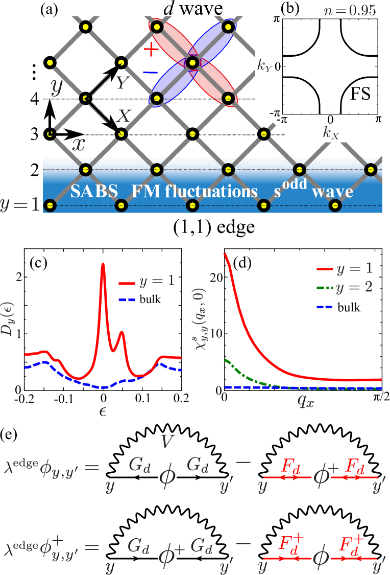
Figure 1: (a) Cluster Hubbard model with a (1,1) edge. The orthogonal unit vectors ($\hat{\bm{x}}$, $\hat{\bm{y}}$) and ($\hat{\bm{X}},\hat{\bm{Y}}$) are illustrated. (b) Bulk FS. (c) SABS-induced peak in the LDOS at $\Delta^{d}=0.16$ in the case with quasiparticle damping $\gamma=0.01$. (d) Edge-induced FM fluctuations obtained via the site-dependent RPA $\chi^{s}_{y,y}(q_{x},0)$ for $T=0.05$ and $\Delta^{d}=0.10$. (e) Linearized edge gap ($\phi^{(+)}$) equation composed of Green’s functions, $G_{d}$ and $F_{d}$, for $\Delta^{d}\neq 0$. $\lambda^{\rm edge}$ is the eigenvalue. The second terms on the right-hand side determine the phase difference between $\Delta^{d}$ and $\phi$ ($\phi^{+})$.

The Hamiltonian is expressed as:

$$\mathcal{H}=H_{0}+U\sum_{i}n_{i\uparrow}n_{i\downarrow}+\sum_{i,j}\Delta_{i,j}^{d}\left(c_{i\uparrow}^{\dagger}c_{j\downarrow}^{\dagger}+{\rm H.c}\right),$$ (1)

where $U$ denotes the on-site Coulomb interaction. $H_{0}=\sum_{i,j,\sigma}t_{i,j}c_{i\sigma}^{\dagger}c_{j\sigma}$ represents the kinetic term, where $t_{i,j}$ denotes the hopping integral between sites $i$ and $j$. In this study, we set $(t_{1},t_{2},t_{3})=(-1,1/6,-1/5)$, where $t_{n}$ is the $n$-th nearest neighbor hopping integral and it corresponds to the ${\rm Y}{\rm Ba}_{2}{\rm Cu}_{3}{\rm O}_{7-x}$ (YBCO) model [18, 19, 20, 69]. The energy unit is $|t_{1}|=1$. The Fermi surface (FS) in the periodic system is illustrated in Fig. 1 (b). $\Delta_{i,j}^{d}$ is the bulk $d_{xy}$ wave ($d_{X^{2}-Y^{2}}$ wave) gap function given as $\Delta_{i,j}^{d}=(\Delta^{d}/4)(\delta_{\bm{r}_{i}-\bm{r}_{j},\pm\hat{\bm{X}}}-\delta_{\bm{r}_{i}-\bm{r}_{j},\pm\hat{\bm{Y}}})$. A similar bulk $d$ wave gap function is microscopically obtained based on spin-fluctuation theories. Considering this fact, we introduce $\Delta^{d}$ as the model parameter to simplify the discussion. To reproduce the suppression of the $d$ wave gap near the edge, we multiplied the $d$ wave gap function by the decay factor $\{1-\exp[(y_{i}+y_{j}-2)/2\xi_{d}]\}$ [20]. Then, we set the coherence length $\xi_{d}=10$. Figure 1 (c) presents the LDOS at the edge site for $\Delta^{d}=0.16$. The obtained sharp SABS-induced peak in LDOS drives the system towards a strong correlation [19]. In the following numerical study, we set the filling as $n=0.95$. The numerical results are essentially unchanged for $n=0.8$–$1.2$.

In this study, we introduce the $2N_{y}\times 2N_{y}$ Nambu Green’s function in the presence of the bulk $d$ wave gap $\Delta_{y,y^{\prime}}^{d}(k_{x})\equiv{\Delta^{d}}^{\uparrow\downarrow}_{y,y^{\prime}}(k_{x})$. Since we assume that $\Delta_{i,j}^{d}$ is real, $\left\{\Delta_{y^{\prime},y}^{d}(k_{x})\right\}^{*}=\Delta_{y,y^{\prime}}^{d}(k_{x})$ is satisfied. Thus, we consider the following Nambu Hamiltonian [19, 20]:

$$\mathcal{H}_{d} =\sum_{k_{x}}\left({}^{t}\hat{c}_{k_{x},\uparrow}^{{\dagger}},^{t}\hat{c}_{-k_{x},\downarrow}\right)\left(\begin{array}[]{cc}\hat{H}^{0}(k_{x})&\hat{\Delta}^{d}(k_{x})\\ \hat{\Delta}^{d}(k_{x})&-^{t}\hat{H}^{0}(-k_{x})\\ \end{array}\right)$$ (4)

$$~{}~{}~{}~{}\times\left(\begin{array}[]{c}\hat{c}_{k_{x},\uparrow}\\ \hat{c}_{-k_{x},\downarrow}^{{\dagger}}\\ \end{array}\right),$$ (7)

where $\hat{c}_{k_{x},\uparrow}$ and $\hat{c}_{-k_{x},\downarrow}^{{\dagger}}$ represent the $N_{y}$-component column vector of sites. Next, we define the Green’s functions in the bulk $d$ wave SC state as follows:

$$\left(\begin{array}[]{cc}\hat{G}_{d}(k_{x},i\epsilon_{n})&\hat{F}_{d}(k_{x},i\epsilon_{n})\\ \hat{F}^{+}_{d}(k_{x},i\epsilon_{n})&-^{t}\hat{G}_{d}(-k_{x},-i\epsilon_{n})\end{array}\right)$$ (10)

$$=\left(\begin{array}[]{cc}i\epsilon_{n}\hat{1}-\hat{H}^{0}(k_{x})&-{\hat{\Delta}}^{d}(k_{x})\\ -{\hat{\Delta}}^{d}(k_{x})&i\epsilon_{n}\hat{1}+^{t}\hat{H}^{0}(-k_{x})\end{array}\right)^{-1}.$$ (13)

Then, we calculate the site-dependent spin susceptibility $\chi^{s}_{y,y^{\prime}}(q_{x},i{\omega}_{l})$ in the cluster Hubbard model with the bulk $d$ wave gap in Eq. (1), using the real-space random-phase-approximation (RPA). Here, we adopt the $k_{x}$ representation by considering the translational symmetry, and ${\omega}_{l}=2\pi Tl$ represents the boson Matsubara frequency. The irreducible susceptibilities are given by $\hat{G}_{d}$, $\hat{F}_{d}$, and $\hat{F}_{d}^{+}$ as

$$\chi^{0}_{y,y^{\prime}}({q}_{x},i\omega_{l}) = -T\sum_{{k}_{x},n}{G_{d}}_{y,y^{\prime}}({q}_{x}+{k}_{x},i\omega_{l}+i\epsilon_{n})$$ (14)

$$\times{G_{d}}_{y^{\prime},y}({k}_{x},i\epsilon_{n}),$$

$$\varphi^{0}_{y,y^{\prime}}(q_{x},i\omega_{l}) = -T\sum_{k_{x},n}{F_{d}}_{y,y^{\prime}}(q_{x}+k_{x},i\omega_{l}+i\epsilon_{n})$$ (15)

$$\times{F_{d}}_{y^{\prime},y}^{+}(k_{x},i\epsilon_{n}).$$

$\varphi^{0}$ is finite only in the SC state. The $N_{y}\times N_{y}$ matrix of the spin (charge) susceptibility $\hat{\chi}^{s(c)}$ is calculated using $\hat{\chi}^{0}$ and $\hat{\varphi}^{0}$ as

$$\hat{\chi}^{0s(c)}(q_{x},i\omega_{l})=\hat{\chi}^{0}(q_{x},i\omega_{l})+(-)\hat{\varphi}^{0}(q_{x},i\omega_{l}),$$ (16)

$$\hat{\chi}^{s(c)}(q_{x},i\omega_{l}) = \hat{\chi}^{0s(c)}(q_{x},i\omega_{l})$$ (17)

$$\times\left\{\hat{1}-(+)U\hat{\chi}^{0s(c)}(q_{x},i\omega_{l})\right\}^{-1}.$$

The spin Stoner factor is the largest eigenvalue of $U\hat{\chi}^{0s}(q_{x},i\omega_{l})$ at $\omega_{l}=0$. The magnetic order is realized when $\alpha_{S}\geq 1$. The pairing interaction for the triplet SC is given by

$$\hat{V}({q}_{x},i\omega_{l})=U^{2}\left(-\frac{1}{2}\hat{\chi}^{s}({q}_{x},i\omega_{l})-\frac{1}{2}\hat{\chi}^{c}({q}_{x},i\omega_{l})\right).$$

(18)

Figure 1(d) illustrates the obtained $\chi^{s}_{y,y}(q_{x},0)$ in the $y$th layer at zero frequency. The obtained strong FM fluctuations ($q_{x}\approx 0$) originate from the SABS [19], and they mediate the spin-triplet edge-induced superconductivity [20].

The linearized triplet gap equations for $\hat{\phi}(k_{x},i{\epsilon}_{n})\ (\propto\langle c_{k_{x}\uparrow}c_{-k_{x}\downarrow}\rangle)$ and $\hat{\phi}^{+}(k_{x},i{\epsilon}_{n})\ (\propto\langle c_{-k_{x}\downarrow}^{\dagger}c_{k_{x}\uparrow}^{\dagger}\rangle)$ are presented in Fig. 1(e), and their analytic expressions are

$$\lambda^{\rm edge}\phi_{y,y^{\prime}}(k_{x},i\epsilon_{n})$$ (19)

$$= -T\sum_{k_{x}^{\prime},Y,Y^{\prime},m}V_{y,y^{\prime}}(k_{x}-k_{x}^{\prime},i\epsilon_{n}-i\epsilon_{m})$$

$$\times\left\{G_{y,Y}(k_{x}^{\prime},i\epsilon_{m})\phi_{Y,Y^{\prime}}(k_{x}^{\prime},i\epsilon_{m})G_{y^{\prime},Y^{\prime}}(-k_{x}^{\prime},-i\epsilon_{m})\right.$$

$$-\left.F_{y,Y}(k_{x}^{\prime},i\epsilon_{m}){\phi^{+}_{Y,Y^{\prime}}}(k_{x}^{\prime},i\epsilon_{m})F_{Y^{\prime},y^{\prime}}(k_{x}^{\prime},i\epsilon_{m})\right\},$$

$$\lambda^{\rm edge}{\phi^{+}_{y,y^{\prime}}}(k_{x},i\epsilon_{n})$$ (20)

$$= -T\sum_{k_{x}^{\prime},Y,Y^{\prime},m}V_{y,y^{\prime}}(k_{x}-k_{x}^{\prime},i\epsilon_{n}-i\epsilon_{m})$$

$$\times\left\{G_{Y,y}(-k_{x}^{\prime},-i\epsilon_{m}){\phi^{+}_{Y,Y^{\prime}}}(k_{x},i\epsilon_{m}^{\prime})G_{Y^{\prime},y^{\prime}}(k_{x}^{\prime},i\epsilon_{m})\right.$$

$$-\left.F_{y,Y}^{+}(k_{x}^{\prime},i\epsilon_{m})\phi_{Y,Y^{\prime}}(k_{x}^{\prime},i\epsilon_{m})F_{Y^{\prime},y^{\prime}}^{+}(k_{x}^{\prime},i\epsilon_{m})\right\}.$$

(We did not study the singlet gap equation because FM fluctuations suppress spin-singlet gaps.) Because the spin-orbit interaction was absent, we assumed that $\bm{d}\parallel\bm{z}$ ($S_{z}^{\rm triplet}=0$) in the triplet gap without the loss of generality. A detailed derivation is presented in Appendix A. Based on Ref. [20], we derived the even-frequency $p$ wave triplet gap $\hat{\phi}(k_{x},i{\epsilon}_{n})=\hat{\phi}(k_{x},-i{\epsilon}_{n})$, where ${\epsilon}_{n}=(2n+1)\pi T$. However, this is not a unique possibility because the odd-frequency pairing state $\hat{\phi}(k_{x},i{\epsilon}_{n})=-\hat{\phi}(k_{x},-i{\epsilon}_{n})$ is not prohibited in principle.

III Numerical Results

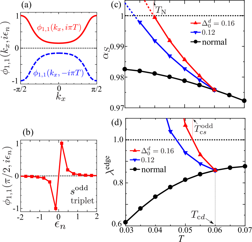
Figure 2: Obtained $s^{\scriptsize\mbox{odd}}$ wave triplet gap at the edge: (a) $\phi_{1,1}(k_{x},\pm i\pi T)$ in the first BZ $(-\pi/2<k_{x}\leq\pi/2)$ and (b) $\phi_{1,1}(k_{x}=\pi/2,i{\epsilon}_{n})$ in the $\Delta_{0}^{d}=0.16$ case at $T=0.05$. Obtained $T$-dependences of (c) the Stoner factor ${\alpha}_{S}$ and (d) the eigenvalue $\lambda^{\rm edge}$ for the $s^{\scriptsize\mbox{odd}}$ wave state. Here, the bulk $d$ wave SC gap appears at $T_{{\rm c}d}=0.06$. In addition, $2\Delta_{0}^{d}/T_{{\rm c}d}=4.0$–$5.3$ for $\Delta_{0}^{d}=0.12$–$0.16$. The edge $s^{\scriptsize\mbox{odd}}$ wave gap is obtained for ${\alpha}_{S}\gtrsim 0.95$ at $T=T_{{\rm c}d}$.

In the triplet state, the even-frequency (odd-frequency) gap exhibits an odd (even) parity in space due to fermion anticommutation relations. Considering both possibilities equally, we analyze the gap equation in Fig. 1 (e) by considering the $i{\epsilon}_{n}$ dependence of $\hat{\phi}(k_{x},i{\epsilon}_{n})$ comprehensively. Here, we assume the Hermitian odd-frequency gap function [28, 27]:

$$\phi_{y,y^{\prime}}^{+}(k_{x},i{\epsilon}_{n})=[\phi_{y^{\prime},y}(k_{x},-i{\epsilon}_{n})]^{*}$$ (21)

The reliability of this relationship will be clarified later. We assumed the BCS-type bulk gap function $\Delta^{d}(T)=\Delta^{d}_{0}\tanh(1.74\sqrt{T_{{\rm c}d}/T-1})$ with the transition temperature $T_{{\rm c}d}=0.06$, which corresponds to $\sim 100$ K in cuprates for $z|t_{1}|\sim 1500$ K with $z=m/m^{*}\sim 0.3$. Experimentally, $4<2\Delta_{0}^{d}/T_{{\rm c}d}<10$ in YBCO [77, 78]. Thus, we set $\Delta_{0}^{d}=0.12$ or $0.16$, which corresponds to $2\Delta_{0}^{d}/T_{{\rm c}d}=4.0$–$5.3$. We set $U=2.32$, where the spin Stoner factor ${\alpha}_{S}$ is $0.975$ at $T=T_{{\rm c}d}$.

III.1 $s^{\rm odd}$ wave SC state

Figures 2(a) and 2(b) exhibit the $k_{x}$ and $i{\epsilon}_{n}$ dependences of the odd-frequency $s$ wave ($s^{\scriptsize\mbox{odd}}$ wave) gap for $\Delta_{0}^{d}=0.16$ at $T=0.05$, respectively. Here, the odd-frequency $s^{\scriptsize\mbox{odd}}$ wave state is obtained as the largest eigenvalue state. At the edge, the pure $s^{\scriptsize\mbox{odd}}$ gap function is obtained because the $d$ wave gap is zero at $y=1$.

Figures 2(c) and 2(d) exhibit the obtained spin Stoner factor ${\alpha}_{S}$ and the eigenvalue $\lambda^{\rm edge}$ as a function of $T$, respectively. Since SC susceptibility is proportional to $1/|1-\lambda^{\rm edge}|$, the edge-gap function is expected to appear when $\lambda^{\rm edge}\sim 1$. In the normal state ($\Delta_{0}^{d}=0$), $\lambda^{\rm edge}$ decreases at low $T$ because the pairing interaction for the odd-frequency SC gap is proportional to $T\chi^{s}({{\bm{q}}}_{x},0)\propto T/(1-{\alpha}_{S})$ [34, 35, 30, 36, 37, 38]. This is a well-known difficulty of the spin-fluctuation-mediated odd-frequency SC mechanism in bulk systems. In contrast, in the presence of the SABS, ${\alpha}_{S}$ increases rapidly due to the huge LDOS at zero energy [70, 19]. Therefore, $\lambda^{\rm edge}$ rapidly approaches unity owing to the SABS-induced magnetic criticality [20]. Thus, the SABS-driven odd-frequency SC mechanism is naturally realized at the edge of $d$ wave superconductors.

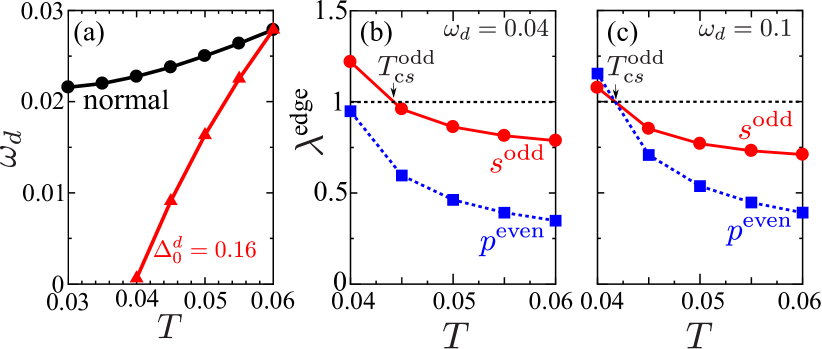
Figure 3: (a) Obtained energy-scale of the dynamical spin susceptibility ${\omega}_{d}\ (\propto 1-{\alpha}_{S})$ as a function of $T$. Eigenvalues $\lambda^{\rm edge}$ obtained by the pairing interaction ${\hat{\chi}}^{s}(q_{x},0)\Omega({\omega}_{l};{\omega}_{d})$ for (b) ${\omega}_{d}=0.04$ and (c) $0.1$. As it approaches the magnetic criticality ${\omega}_{d}\rightarrow 0$, $T_{{\rm c}s}^{\scriptsize\mbox{odd}}$ increases whereas $T_{{\rm c}p}^{\scriptsize\mbox{even}}$ decreases. In (b), $T_{{\rm c}s}^{\scriptsize\mbox{odd}}$ is higher than $T_{{\rm c}p}^{\scriptsize\mbox{even}}$.

III.2 $s^{{\scriptsize\mbox{odd}}}$ wave SC state dominates $p^{\scriptsize\mbox{even}}$ wave SC state

Here, we discuss the reason behind the edge $s^{\scriptsize\mbox{odd}}$ wave state dominating the edge even-frequency $p^{\scriptsize\mbox{even}}$ wave state in this study. In the $k_{x}$-space argument, the larger condensation energy is expected in the nodeless $s^{\scriptsize\mbox{odd}}$ wave state. In the ${\epsilon}_{n}$-space argument, proximity to the magnetic criticality (${\alpha}_{S}\lesssim 1$) is crucial: The edge pairing interaction $V_{1,1}(q_{x},i{\omega}_{l})\propto\chi^{s}_{1,1}(q_{x},i{\omega}_{l})$ at $q_{x}\sim 0$ is well fitted by the function $\Omega({\omega}_{l};{\omega}_{d})={\omega}_{d}/(|{\omega}_{l}|+{\omega}_{d})$, and the obtained ${\omega}_{d}$ in the present real-space RPA study is presented in Fig. 3 (a). ${\omega}_{d}\ (\propto 1-{\alpha}_{S})$ approaches zero at the magnetic critical point, and the eigenvalues of even- and odd-frequency solutions become similar [34, 35, 30, 36, 37, 38]. To verify this discussion, we compare the eigenvalues $\lambda^{\rm edge}$ of both $s^{\scriptsize\mbox{odd}}$ wave and $p^{\scriptsize\mbox{even}}$ wave states, by introducing a separable pairing interaction $V_{y,y^{\prime}}(q_{x},i{\omega}_{l})\propto\chi^{s}_{y,y^{\prime}}(q_{x},0)\Omega({\omega}_{l};{\omega}_{d})$. The obtained results are presented in Figs. 3(b) and 3(c) for ${\omega}_{d}=0.04$ and ${\omega}_{d}=0.1$, respectively. It is verified that the $s^{\scriptsize\mbox{odd}}$ wave dominates the $p^{\scriptsize\mbox{even}}$ wave near the quantum criticality ${\omega}_{d}=0.04$, which corresponds to the RPA study demonstrated in Fig. 2. The obtained $s^{\scriptsize\mbox{odd}}$ wave state should be robust against impurity scattering according to the Anderson theorem.

The obtained edge $s^{\scriptsize\mbox{odd}}$ wave gap in the ${\epsilon}_{n}$ representation is real in the case of $\Delta^{d}={\rm real}$. That is, $\phi_{1,1}(k_{x},i{\epsilon}_{n})\propto{\epsilon}_{n}$ is real for small ${\epsilon}_{n}$. Then, after the analytic continuation, $\phi^{\prime}=[\phi_{1,1}^{\rm R}(k_{x},{\epsilon})+\phi_{1,1}^{\rm A}(k_{x},{\epsilon})]/2\propto i{\epsilon}$ becomes purely imaginary. In addition, the triplet gap function is odd with respect to the time reversal. Therefore, the obtained state is the TRS “$d+s^{\scriptsize\mbox{odd}}$ wave state.” Because $\phi^{\prime\prime}=[\phi_{1,1}^{\rm R}(k_{x},0)-\phi_{1,1}^{\rm A}(k_{x},0)]/2$ also approaches zero near the magnetic criticality [30], the edge $s^{\scriptsize\mbox{odd}}$ wave gap will not affect the LDOS at zero-energy. This result is consistent with the ubiquitous presence of the zero-bias conductance peak in the tunneling spectroscopy of cuprates [10, 11, 79, 80]

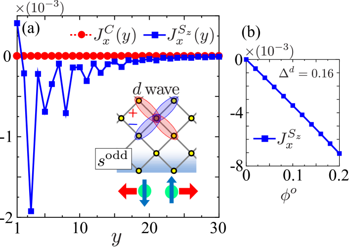
Figure 4: (a) Obtained edge currents in the $d+s^{\scriptsize\mbox{odd}}$ state derived from the edge gap equation shown in Fig. 1 (e). Here, $d=d_{xy}$. The edge currents in the $p+is^{\scriptsize\mbox{odd}}$, $d+is^{\scriptsize\mbox{even}}$, and $p+s^{\scriptsize\mbox{even}}$ states are illustrated in Appendix Dand listed in Table 1. Here, we set $\Delta^{d}=0.16$ while the $s^{\scriptsize\mbox{odd}}$ wave gap function is set as $\phi_{y,y^{\prime}}(i{\epsilon}_{n})=\phi^{\rm o}f^{\rm o}({\epsilon}_{n})\delta_{y,1}\delta_{y^{\prime},1}$ with $\phi^{\rm o}=0.16$, where $f^{\rm o}({\epsilon}_{n})$ is given in Fig. 2 (b). (b) Obtained total edge current $J_{x}^{{\rm S}z}$ for $\Delta^{d}=0.16$ as a function of $\phi^{\rm o}$.

III.3 Edge super current

Here, we elucidate the emergence of the nontrivial edge supercurrent in the $d+s^{\scriptsize\mbox{odd}}$ wave state. In the present cluster model with the $d+s^{\scriptsize\mbox{odd}}$ wave gap, the charge current along the $x$ axis from layer $y$ [Fig. 1(a)] to any layer is calculated as

$$J_{x}^{\rm C}(y) = \sum_{k_{x},y^{\prime},\sigma,\rho}\big{\{}(-e\delta_{{\sigma},\rho})v_{x}(k_{x},y,y^{\prime})$$ (22)

$$\times\mathcal{G}_{y^{\prime},y}^{{\sigma},\rho}(k_{x},i{\epsilon}_{n})e^{-i{\epsilon}_{n}0}+(y\leftrightarrow y^{\prime})\big{\}},$$

where $v_{x}(k_{x},y,y^{\prime})\equiv{\partial}H_{y,y^{\prime}}^{0}(k_{x})/{\partial}k_{x}$ [81] and $\mathcal{G}_{y^{\prime},y}^{{\sigma},\rho}$ presents the Green’s function for the $d+s^{\scriptsize\mbox{odd}}$ state in Appendix A. Here, we set $\phi_{y,y^{\prime}}(i{\epsilon}_{n})=\phi^{\rm o}f^{\rm o}({\epsilon}_{n})\delta_{y,1}\delta_{y^{\prime},1}$, with $\phi^{\rm o}=\Delta_{0}^{d}=0.16$, where $f^{\rm o}({\epsilon}_{n})$ is provided in Fig. 2 (b). The numerical results obtained are insensitive to the parameters $\phi^{\rm o}$ and $\Delta_{0}^{d}=0.16$. Accordingly, the total edge current is $J_{x}^{\rm C}=\sum_{y}J_{x}^{\rm C}(y)$. We also calculate the spin current along the $x$ axis $J_{x}^{{\rm S}\mu}(y)$, where $\mu$ represents the spin current polarization. It is obtained by replacing $(-e\delta_{{\sigma},\rho})$ with $(\hbar\hat{{\sigma}}^{\mu}_{{\sigma},\rho})$ in Eq. (22), where $\hat{{\sigma}}^{\mu}$ depicts the Pauli matrix. Because $s_{z}$ is conserved in the present SC state, $J_{x}^{{\rm S}\mu}(y)$ is zero for $\mu=x,y$. We emphasize that $J_{x}^{{\rm S}\mu}(y)$ remains constant under the time reversal.

Figure 4(a) presents the obtained currents in the $d+s^{\scriptsize\mbox{odd}}$ wave state by setting $e=\hbar=1$. Here, the charge current $J_{x}^{\rm C}(y)$ vanishes identically, which is consistent with the experimental reports of muon spin rotation ($\mu$-SR) [82]; however, the non zero spin current $J_{x}^{{\rm S}z}(y)$ flows spontaneously. The spin current polarization is parallel to the $\bm{d}$ vector. Here, the parity of the mirror operation ${\cal M}_{x}$ is odd because the $d_{xy}$ ($s^{\scriptsize\mbox{odd}}$) gap has odd (even) parity. In addition, the spin exchange parity is $-1$. Consequently, conduction electrons acquire spin-dependent velocity, and therefore, $J_{x}^{{\rm S}z}(y)\neq 0$. The obtained total spin current $J_{x}^{{\rm S}z}\equiv\sum_{y}J_{x}^{{\rm S}z}(y)$ is $\phi^{\rm o}$ linear, as shown in Fig. 4 (b). Because $J_{x}^{{\rm S}z}$ is linear in $|\phi^{\rm o}|$, a sizable amount of spin current is expected.

Furthermore, we also study the edge currents in the $d+is^{\scriptsize\mbox{even}}$, $p+is^{\scriptsize\mbox{odd}}$, and $p+s^{\scriptsize\mbox{even}}$ wave states. In the TRS breaking $p+is^{\scriptsize\mbox{odd}}$ wave state ($p=p_{x}$), we find that the finite charge current emerges as shown in Fig. 5 (a), whereas spin current vanishes. In the $p+is^{{\scriptsize\mbox{odd}}}$ wave state, the parity of ${\cal M}_{x}$ is odd, while the parity of the spin part is even. As a result, $J_{x}^{\rm C}\neq 0$ is realized. The present study is a nontrivial extension of the theory of the $d+is^{\scriptsize\mbox{even}}$ wave state [14].

We notice that, when the bulk SC gap is $p_{x}$ wave, the SABS that drives the edge $s^{\scriptsize\mbox{odd}}$ wave state is absent [7]. In the $p_{X}$ wave SC state, the SABS exists, and the parity of ${\cal M}_{x}$ is not completely even. Therefore, the $p_{X}$ wave SC state is favorable to realize the odd-frequency SC state with a finite edge current. The $p_{X}$ wave can be realized by applying the uniaxial strain in the chiral or helical $p$ wave state.

Next, we calculate the edge-induced currents due to the edge even-frequency $s$ wave states. Figures 5(b) and 5(c) are the obtained edge currents in the $d+is^{\scriptsize\mbox{even}}$ wave and $p+s^{\scriptsize\mbox{even}}$ wave states, respectively. The obtained charge current in Fig. 5 (b) is consistent with the Matsumoto-Shiba theory [14]. The parities and edge currents in the edge odd- and even-frequency SC states are summarized in Table I.

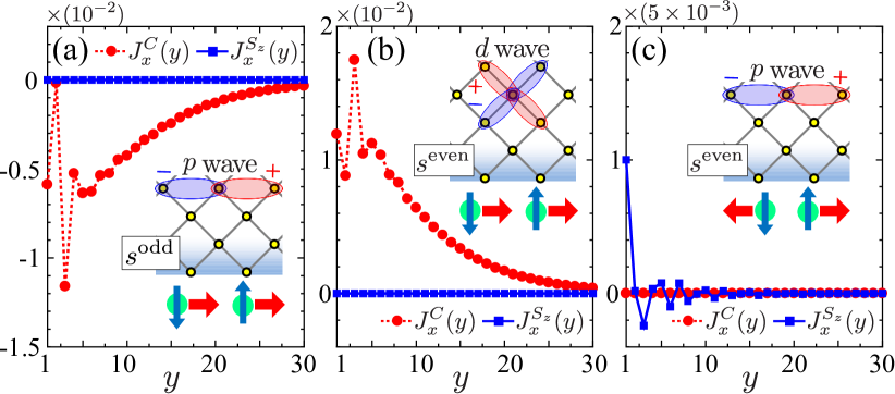
Figure 5: Obtained edge currents in (a) the $p+is^{\scriptsize\mbox{odd}}$ wave state, (b) the $d+is^{\scriptsize\mbox{even}}$ wave state, and (c) the $p+s^{\scriptsize\mbox{even}}$ wave state. Here, $p=p_{x}$, $d=d_{xy}$, and $\Delta^{p,d}=0.16$. We set the $s^{\scriptsize\mbox{odd}}$ wave gap function as $\phi_{y,y^{\prime}}(i{\epsilon}_{n})=\phi^{\rm o}f^{\rm o}({\epsilon}_{n})\delta_{y,1}\delta_{y^{\prime},1}$ with $\phi^{\rm o}=0.16$, where $f^{\rm o}({\epsilon}_{n})$ is given in Fig. 2(b). We also set the $s^{\scriptsize\mbox{even}}$ wave gap $\phi_{y,y^{\prime}}(i{\epsilon}_{n})=\phi^{\rm e}\delta_{y,1}\delta_{y^{\prime},1}$ with $\phi^{\rm e}=0.16$.

Table 1: Parities and edge currents in $d+s^{\scriptsize\mbox{odd}}$ $p+is^{\scriptsize\mbox{odd}}$, $d+is^{\scriptsize\mbox{even}}$, and $p+s^{\scriptsize\mbox{even}}$ wave states for $d=d_{xy}$ and $p=p_{x}$. These states satisfy ${\cal M}_{x}=-1$. All currents disappear if the phase of the edge gap is shifted by $\pi/2$. No currents flow for $d=d_{x^{2}-y^{2}}$ and $p=p_{y}$ because ${\cal M}_{x}=+1$.

SC state	Time-reversal	Spin exchange	$J_{x}^{\rm C}$	$J_{x}^{{\rm S}z}$
$d+s^{\scriptsize\mbox{odd}}$	$+$	$-$	0	non zero
$p+is^{\scriptsize\mbox{odd}}$	$-$	$+$	non zero	0
$d+is^{\scriptsize\mbox{even}}$	$-$	$+$	non zero	0
$p+s^{\scriptsize\mbox{even}}$	$+$	$-$	0	non zero

IV relationship between $\phi$ and $\phi^{+}$

Finally, we discuss a fundamental open problem in the relationship between $\phi$ and $\phi^{+}$ in the odd-frequency gap function. In this study, we assume the relationship in Eq. (21), which is directly derived from the Lehmann representation. This relationship gives the para-Meissner effect, and therefore, it is not as stable as a bulk SC state. Nonetheless, the odd-frequency gap function is naturally expected as the edge-state of bulk superconductivity. However, a different non-Hermitian relationship, ${\bar{\phi}}_{y,y^{\prime}}^{+}(k_{x},i{\epsilon}_{n})=[\phi_{y^{\prime},y}(k_{x},+i{\epsilon}_{n})]^{*}$, proposed in Refs. [22, 31, 32, 33], which exhibits the usual Meissner effect, inevitably induces imaginary spin current in the $d+s^{\scriptsize\mbox{odd}}$ wave state, as demonstrated in this study. Therefore, the Hermitian relationship (21) should be the true equation.

To determine the edge $s^{\scriptsize\mbox{odd}}$ gap function, it is beneficial to focus on the anomalous proximity effect in a diffusive normal metal (DNM), where the quasiparticle in the DNM exhibits a zero-energy peak of the LDOS [57]. In the absence of the edge $s^{\scriptsize\mbox{odd}}$ gap function, the odd-frequency singlet $p$ wave is solely induced at the interface; however, it cannot penetrate into the DNM. Once the $s^{\scriptsize\mbox{odd}}$ triplet SC state is induced, it can penetrate into the DNM and generate the zero-energy peak of the LDOS.

V summary

We have predicted that an odd-frequency spin-triplet $s$ wave gap function emerges at the edge of $d$ wave superconductors, mediated by the zero-energy SABS-induced ferromagnetic fluctuations. This prediction is obtained from the analysis of the edge SC gap equation based on the cluster Hubbard model with a bulk $d$ wave gap. The predicted odd-frequency $s$ wave gap function is expected to be robust against randomness. The obtained SC state with the TRS accompanies the spontaneous edge spin current. The predicted edge spin current in the $d+s^{\scriptsize\mbox{odd}}$ wave state is a useful signal for detecting the hidden odd-frequency SC gap function. We also provided decisive validation of the Hermitian relationship [Eq. (21)] of the odd-frequency gap function. An important future issue is to analyze the electronic states below $T_{{\rm c}s}^{\scriptsize\mbox{odd}}$ by considering strong coupling effects, like the self-energy and feedback effects.

We have revealed that SABS-driven spin fluctuations at the edge of the bulk superconductor induce an exotic edge superconductivity. The SABS-driven spin fluctuations will also induce exotic edge charge density wave (CDW) due to the paramagnon interference mechanism [83, 84, 85, 86, 87]. The $d$ wave bond order [75, 76, 88], $p$ wave charge current order [89], and $p$ wave spin current order [90] are expected to be realized by the paramagnon interference mechanism [91]. The emergence of an edge-induced exotic CDW is an important future issue.

Appendix A Linearized gap equation for the edge-induced triplet states

In this appendix, we derive the linearized triplet gap equation in the presence of the bulk $d$ wave gap [20]. First, we assume that $\Delta_{y,y^{\prime}}^{d}(k_{x})$ and the edge triplet gap $\phi_{y,y^{\prime}}(k_{x},i\epsilon_{n})\equiv\phi^{\uparrow\downarrow}_{y,y^{\prime}}(k_{x},i\epsilon_{n})$ are both finite. We ignore the spin orbit interaction, so we can set the $\bm{d}$ vector as $\hat{{\bm{d}}}=(0,0,\hat{\phi})$. Then, we define the $2N_{y}\times 2N_{y}$ Green’s functions $\hat{\mathcal{G}}_{\rm Nam}$ in the bulk+edge SC state as follows:

$$\hat{\mathcal{G}}_{\rm Nam}\equiv\left(\begin{array}[]{cc}\hat{\mathcal{G}}^{\uparrow\uparrow}(k_{x},i\epsilon_{n})&\hat{\mathcal{F}}^{\uparrow\downarrow}(k_{x},i\epsilon_{n})\\ \hat{\mathcal{F}^{+}}^{\uparrow\downarrow}(k_{x},i\epsilon_{n})&-{{}^{t}\hat{\mathcal{G}}^{\downarrow\downarrow}(-k_{x},-i\epsilon_{n})}\\ \end{array}\right)$$ (25)

$$\ \ \ =\left(\begin{array}[]{cc}i\epsilon_{n}-\hat{H}^{0}(k_{x})&-\hat{\Delta}^{d}(k_{x})-\hat{\phi}(k_{x},i\epsilon_{n})\\ -\hat{\Delta}^{d}(k_{x})-\hat{\phi}^{+}(k_{x},i\epsilon_{n})&i\epsilon_{n}+{{}^{t}\hat{H}^{0}}(-k_{x})\\ \end{array}\right)^{-1}.$$ (28)

The equation for the triplet gap $\phi_{y,y^{\prime}}(k_{x},i\epsilon_{n})$ is given by

$$\phi_{y,y^{\prime}}(k_{x},i\epsilon_{n})=T\sum_{k_{x}^{\prime},m} V_{y,y^{\prime}}(k_{x}-k_{x}^{\prime},i\epsilon_{n}-i\epsilon_{m})$$

$$\times \mathcal{F}_{y,y^{\prime}}^{\rm triplet}(k_{x}^{\prime},i\epsilon_{m}),$$ (29)

where $\hat{\mathcal{F}}^{\rm triplet}(k_{x},i\epsilon_{n})\equiv\{\hat{\mathcal{F}}^{\uparrow\downarrow}(k_{x},i\epsilon_{n})+\hat{\mathcal{F}}^{\downarrow\uparrow}(k_{x},i\epsilon_{n})\}/2$ is the triplet part of the anomalous Green’s function in the coexisting SC state. In order to linearize (29), we evaluate $\hat{\mathcal{F}}^{\rm triplet}$ by the first-order perturbation of $\hat{\phi}$ and $\hat{\phi}^{+}$ to the Green’s functions (13). Since $\hat{F}_{d}$ satisfies the relation $\hat{F}_{d}^{\uparrow\downarrow}=-\hat{F}_{d}^{\downarrow\uparrow}$, we obtain $\hat{\mathcal{F}}^{\rm triplet}=-\hat{G}_{d}\hat{\phi}\hat{\bar{G}}_{d}+\hat{F}_{d}\hat{\phi}^{+}\hat{F}_{d}$, where $\hat{\bar{G}}_{d}\equiv{{}^{t}\hat{G}_{d}}(-k_{x},-i\epsilon_{n})$. By substituting it into Eq. (29), we obtain the analytic expression of the linearized triplet gap equation for $\hat{\phi}$ in Fig. 1(e). The set of Eqs. (19) and (20) gives the linearized triplet gap equation in the presence of the bulk $d$ wave gap. [In Eqs. (19) and (20), the subscript $d$ of $G$ and $F$ is omitted.] The edge triplet SC state appears when the eigenvalue $\lambda^{\rm edge}$ is around unity.

In the main text, we use the Hermitian odd-frequency gap $\phi^{+}(i{\epsilon}_{n})=-[\phi(i{\epsilon}_{n})]^{*}$, and obtain the time-reversal-symmetry $d+s^{\scriptsize\mbox{odd}}$ wave state. We note that the eigenvalue $\lambda^{\rm edge}$ is unchanged even if one assumes a non-Hermitian relation $\phi^{+}(i{\epsilon}_{n})=[\phi(i{\epsilon}_{n})]^{*}$.

In the present study, the Hermitian odd-frequency gap relation gives the finite charge or spin current unless the parity of ${\cal{M}}_{x}$ is even. On the other hand, the non-Hermitian odd-frequency gap relation leads to unphysical imaginary currents in the cases of the $d+is^{\scriptsize\mbox{odd}}$ wave and $p+s^{\scriptsize\mbox{odd}}$ wave states.

Appendix B $k_{x}$ dependence of $s^{{\scriptsize\mbox{odd}}}$ gap

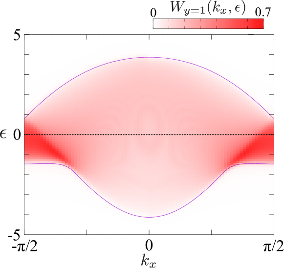
Figure 6: Weight of the edge layer state in the normal state; $W_{y=1}(k_{x},{\epsilon})$.

Figure 6 shows the weight of the edge layer state ($y=1$) in the present cluster tight-binding model without $\Delta^{d}$. It is given as $W_{y}(k_{x},{\epsilon})=\sum_{b}\delta(E_{b,k_{x}}-{\epsilon})|U(y,b,k_{x})|^{2}$, where $E_{b,k_{x}}$ is the $b$-th band energy at $k_{x}$ measured from $\mu$ and $U(y,b,k_{x})$ is the unitary matrix. Note that the relation $D_{y}({\epsilon})=\sum_{k_{x}}W_{y}(k_{x},{\epsilon})$ holds. Since the edge weight is large for $|k_{x}|\sim\pi/2$, the magnitude of the $s^{\scriptsize\mbox{odd}}$ wave gap function in Fig. 2(a) is large for $|k_{x}|\sim\pi/2$.

Appendix C Coherence length of the bulk $d$ wave gap

The $d$ wave gap function in the Hamiltonian is given as $\Delta_{i,j}^{d}=(\Delta^{d}/4)(\delta_{\bm{r}_{i}-\bm{r}_{j},\pm\hat{\bm{X}}}-\delta_{\bm{r}_{i}-\bm{r}_{j},\pm\hat{\bm{Y}}})$. Near the edge layer ($y=1$), $\Delta^{d}_{i,j}$ should be suppressed if the $y$-components of the sites $i$ and $j$, $y_{i}$ and $y_{j}$, are smaller than the coherence length $\xi_{d}=10$. In order to reproduce this suppression, we multiply $\Delta_{i,j}^{d}$ in the Hamiltonian by the decay factor $\{1-\exp[(y_{i}+y_{j}-2)/2\xi_{d}]\}$ [20]. In the main text, we set the coherence length $\xi_{d}=10$, and then $|\Delta_{i,j}^{d}|$ for $i=(x,y)$ and $j=(x+1,y+1)$ is given in Fig. 7. From the experimental results [92, 93, 94, 95], the coherence length in the $a$-$b$ plane of YBCO is 1nm for $T\ll T_{{\rm c}d}$. Therefore, $\xi_{d}=10$ is a reasonable value.

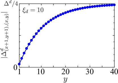
Figure 7: $|\Delta_{i,j}^{d}|$ for $i=(x,y)$ and $j=(x+1,y+1)$ for $\xi_{d}=10$.

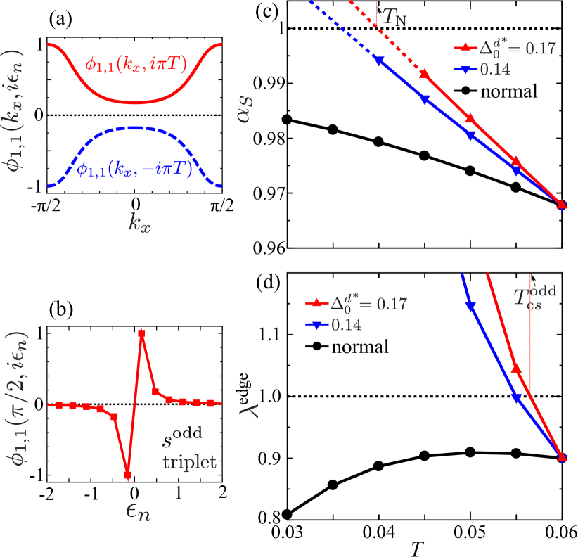
Figure 8: Odd-frequency gap functions obtained by the modified FLEX theory for $U=2.8$. (a)(b) Obtained $s^{\scriptsize\mbox{odd}}$ wave triplet gap at edge: (a) $\phi_{1,1}(k_{x},\pm i\pi T)$ and (b) $\phi_{1,1}(k_{x}=\pi/2,i{\epsilon}_{n})$ in case of ${\Delta_{0}^{d}}^{*}=0.17$ at $T=0.05$. (c)(d) $T$-dependences of (c) the Stoner factor ${\alpha}_{S}$ and (d) the eigenvalue $\lambda^{\rm edge}$ for the $s^{\scriptsize\mbox{odd}}$ wave state. Here, the bulk $d$ wave SC gap appears at $T_{{\rm c}d}=0.06$. $2{\Delta_{0}^{d}}^{*}/T_{{\rm c}d}=4.7$ and 5.6 for ${\Delta_{0}^{d}}^{*}=0.14$ and 0.17, respectively. The edge $s^{\scriptsize\mbox{odd}}$ wave gap is obtained for ${\alpha}_{S}\gtrsim 0.968$ at $T=T_{{\rm c}d}$.

Appendix D Analysis by modified FLEX approximation

In the main text, we calculated the $y,y^{\prime}$-dependence of the pairing interaction $V_{y,y^{\prime}}(k_{x},i{\omega}_{n})$ using the site-dependent RPA theory. Here, we calculate $V_{y,y^{\prime}}(k_{x},i{\omega}_{n})$ using the modified fluctuation-exchange (FLEX) approximation, in order to study the effect of the self-energy effect, by following our previous study [19]. We set $U=2.8$ hereafter.

Figures 8(a) and 8(b) show the $q_{x}$ and ${\omega}_{n}$ dependences of the odd-frequency $s^{\scriptsize\mbox{odd}}$ wave gap at $T=0.05$, respectively. By setting $\Delta_{0}^{d}=0.24$ ($0.20$) in the Hamiltonian, the normalized $d$ wave gap is obtained as ${\Delta_{0}^{d}}^{*}=0.17$ ($0.14$) due to the self-energy in the FLEX approximation [20]. The obtained results are similar to those in Figs. 2(a) and 2(b) in the main text given by the RPA.

Figures 8(c) and 8(d) exhibit the obtained spin Stoner factor ${\alpha}_{S}$ and the eigenvalue $\lambda^{\rm edge}$ as functions of $T$, respectively. In the normal state (${\Delta_{0}^{d}}^{*}=0$), ${\alpha}_{S}$ moderately increases at low temperatures. In contrast, $\lambda^{\rm edge}$ decreases at low $T$ since the pairing interaction for the odd-frequency SC gap is proportional to $T\chi^{s}({{\bm{q}}}_{x},0)$. In contrast, in the presence of the $d$ wave gap ${\Delta_{0}^{d}}^{*}$, ${\alpha}_{S}$ rapidly increases due to the huge zero-energy surface Andreev bound state (SABS) peak. Therefore, $\lambda^{\rm edge}$ rapidly increases owing to the SABS-induced magnetic criticality [20]. These results are similar to those in Figs. 2(c) and 2(d) in the main text.

Thus, the SABS-driven odd-frequency SC state is naturally obtained at the edge of $d$ wave superconductors, even if the self-energy effect is taken into account based on the modified FLEX theory.

References

- [1] L. J. Buchholtz and G. Zwicknagl. Phys. Rev. B, 23, 5788 (1981).
- [2] J.Hara and K.Nagai, Prog. Theor. Phys. 76, 1237 (1986).
- [3] C. R. Hu, Phys. Rev. Lett. 72, 1526 (1994).
- [4] Y. Tanaka and S. Kashiwaya, Phys. Rev. Lett. 74, 3451 (1995).
- [5] S. Kashiwaya, Y. Tanaka, M. Koyanagi, K. Kajimura, Phys. Rev. B 53, 2667 (1996).
- [6] Y. Nagato and K. Nagai, Phys. Rev. B 51, 16254 (1995).
- [7] S. Kashiwaya and Y. Tanaka, Rep. Prog. Phys. 63, 1641 (2000).
- [8] M. Sato, Y. Tanaka, K. Yada, and T. Yokoyama, Phys. Rev. B 83, 224511 (2011).
- [9] S. Kashiwaya, Y. Tanaka, M. Koyanagi, H. Takashima, and K. Kajimura, Phys. Rev. B 51, 1350 (1995).
- [10] L. Alff, H. Takashima, S. Kashiwaya, N. Terada, H. Ihara, Y. Tanaka, M. Koyanagi, and K. Kajimura, Phys. Rev. B 55, R14757 (1997).
- [11] J. Y. T. Wei, N. -C. Yeh, D. F. Garrigus, and M. Strasik, Phys. Rev. Lett. 81, 2542 (1998).
- [12] J. Geerk, X. X. Xi, and G. Linker, Z. Phys. B 73, 329 (1988).
- [13] M. Matsumoto and H. Shiba, J. Phys. Soc. Jpn. 64, 3384 (1995).
- [14] M. Matsumoto and H. Shiba, J. Phys. Soc. Jpn. 64, 4867 (1995).
- [15] K. Kuboki and M. Sigrist, J. Phys. Soc. Jpn. 67, 2873 (1998).
- [16] M Fogelström, D. Rainer, and J. A. Sauls, Phys. Rev. Lett. 79, 281 (1997).
- [17] A. C. Potter and P. A. Lee, Phys. Rev. Lett. 112, 117002 (2014).
- [18] S. Matsubara, Y. Yamakawa, and H. Kontani, J. Phys. Soc. Jpn. 87, 073705 (2018).
- [19] S. Matsubara and H. Kontani, Phys. Rev. B 101, 075114 (2020).
- [20] S. Matsubara and H. Kontani, Phys. Rev. B 101, 235103 (2020).
- [21] V. L. Berezinskii, JETP Lett. 20, 287 (1974).
- [22] T. R. Kirkpatrick and D. Belitz, Phys. Rev. Lett. 66, 1533 (1991); D. Belitz and T. R. Kirkpatrick, Phys. Rev. B 60, 3485 (1999).
- [23] E. Abrahams, A. Balatsky, D. J. Scalapino, and J. R. Schrieffer, Phys. Rev. B 52, 1271 (1995).
- [24] P. Coleman, E. Miranda and A. Tsvelik, Phys. Rev. Lett. 70, 2960 (1993).
- [25] Y. Tanaka, M. Sato, and N. Nagaosa, J. Phys. Soc. Jpn. 81, 011013 (2012).
- [26] J. Linder and A. V. Balatsky, Rev. Mod. Phys. 91, 045005 (2019).
- [27] M. Matsumoto, M. Koga, and H. Kusunose, J. Phys. Soc. Jpn. 82, 034708 (2013).
- [28] Y. V. Fominov, Y. Tanaka, Y. Asano, and M.Eschrig, Phys. Rev. B 91, 144514 (2015).
- [29] S. Hoshino, K. Yada, and Y. Tanaka, Phys. Rev. B 93, 224511 (2016).
- [30] Y. Fuseya, H. Kohno, and K. Miyake, J. Phys. Soc. Jpn. 72, 2914 (2003).
- [31] D. Solenov, I. Martin, and D. Mozyrsky, Phys. Rev. B 79, 132502 (2009).
- [32] H. Kusunose, Y. Fuseya, and K. Miyake, J. Phys. Soc. Jpn. 80, 054702 (2011).
- [33] H. Kusunose, M. Matsumoto, and M. Koga, Phys. Rev. B 85, 174528 (2012).
- [34] N. Bulut, D. J. Scalapino and S. R. White, Phys. Rev. B 47 14599 (1993).
- [35] M. Vojta and E. Dagotto, Phys. Rev. B 59, R713 (1999).
- [36] T. Hotta, J. Phys. Soc. Jpn. 78, 123710 (2009).
- [37] K. Shigeta, S. Onari, K. Yada and Y. Tanaka, Phys. Rev. B 79, 174507 (2009).
- [38] Y. Yanagi, Y. Yamashita, and K. Ueda, J. Phys. Soc. Jpn. 81, (2012) 123701.
- [39] R. Heid, Z. Phys. B 99, 15 (1995).
- [40] S. Hoshino, Phys. Rev. B 90, 115154 (2014).
- [41] F. S. Bergeret, A. F. Volkov, and K. B. Efetov, Phys. Rev. Lett. 86, 4096 (2001); Phys. Rev. B 64, 134506 (2001).
- [42] F. S. Bergeret, A. F. Volkov, and K. B. Efetov, Rev. Mod. Phys. 77, 1321 (2005).
- [43] Ya. V. Fominov, N. M. Chtchelkatchev, and A. A. Golubov Phys. Rev. B 66, 014507 (2002).
- [44] T. Yokoyama, Y. Tanaka, and A. A. Golubov Phys. Rev. B 75, 134510 (2007).
- [45] A. I. Buzdin, Rev. Mod. Phys. 77, 935 (2005).
- [46] A. I. Buzdin, A. S. Mel’nikov, and N. G. Pugach Phys. Rev. B 83, 144515 (2011).
- [47] S. Mironov, A. Mel’nikov, and A. Buzdin Phys. Rev. Lett. 109, 237002 (2012).
- [48] Jacob Linder, Takehito Yokoyama, Asle Sudbø, and Matthias Eschrig Phys. Rev. Lett. 102, 107008 (2009).
- [49] Mohammad Alidoust, Klaus Halterman, and Jacob Linder Phys. Rev. B 89, 054508 (2014).
- [50] M. Eschrig, J. Kopu, J. C. Cuevas, and G. Sch¨on, Phys. Rev. Lett. 90, 137003 (2003).
- [51] Y. Asano, Y. Tanaka, and A. A. Golubov, Phys. Rev. Lett. 98, 107002 (2007).
- [52] J. Cayao, C. Triola, and A. M. Black-Schaffer, Eur. Phys. J. Special Topics 229, 545 (2020).
- [53] Y. Tanaka and A. A. Golubov, Phys. Rev. Lett. 98, 037003 (2007).
- [54] S. Tamura, S. Hoshino, and Y. Tanaka, Phys. Rev. B 99, 184512 (2019).
- [55] Y. Tanaka, A. A. Golubov, S. Kashiwaya, and M. Ueda. Phys. Rev. Lett. 99, 037005 (2007).
- [56] Y. Tanaka, Y. Tanuma, and A. A. Golubov. Phys. Rev. B 76, 054522 (2007).
- [57] Y. Tanaka and S. Kashiwaya: Phys. Rev. B 70 012507 (2004).
- [58] S. Higashitani, Y. Nagato, and K. Nagai, Journal of Low Temperature Physics 155, 83 (2009).
- [59] S. Higashitani: J. Phys. Soc. Jpn. 66 2556 (1997).
- [60] Y. Tanaka, Y. Asano, A. Golubov, and S. Kashiwaya: Phys. Rev. B 72 140503(R) (2005).
- [61] S. Suzuki and Y. Asano, Phys. Rev. B 89, 184508 (2014).
- [62] S. Suzuki and Y. Asano, Phys. Rev. B 91, 214510 (2015).
- [63] A. Di Bernardo, Z. Salman, X. L. Wang, M. Amado, M. Egilmez, M. G. Flokstra, A. Suter, S. L. Lee, J. H. Zhao, T. Prokscha, E. Morenzoni, M. G. Blamire, J. Linder, and J. W. A. Robinson, Phys. Rev. X 5, 041021 (2015).
- [64] J. A. Krieger, A. Pertsova, S. R. Giblin, M. Döbeli, T. Prokscha, C. W. Schneider, A. Suter, T. Hesjedal, A. V. Balatsky, and Z. Salman, Phys. Rev. Lett. 125, 026802 (2020).
- [65] T. Moriya and K. Ueda: Adv. Phys. 49 555 (2000).
- [66] D. J. Scalapino, Rev. Mod. Phys. 84, 1383 (2012).
- [67] Y. M. Vilk, A. -M. S. Tremblay, J. Phys. I France 7, 1309 (1997).
- [68] A. V. Chubukov, D. Pines, and J. Schmalian, Superconductivity: Conventional and Unconventional Superconductors, edited by K.-H. Bennemann and J. B. Ketterson (Springer, Berlin, 2003).
- [69] H. Kontani, Rep. Prog. Phys. 71 (2008) 026501.
- [70] Y. Chen and C. S. Ting, Phys. Rev. Lett. 92, 077203 (2004).
- [71] H. Kontani and M. Ohno, Phys. Rev. B 74, 014406 (2006); J. Magn. Magn. Mater. 310, 483 (2007).
- [72] P. Mendels, J. Bobroff, G. Collin, H. Alloul, M. Gabay, J.F. Marucco, N. Blanchard and B. Grenier, Europhys. Lett. 46 678 (1999).
- [73] K. Ishida, Y. Kitaoka, K. Yamazoe, K. Asayama, and Y. Yamada, Phys. Rev. Lett. 76 531 (1996).
- [74] Y. Yamakawa and H. Kontani, Phys. Rev. Lett. 114, 257001 (2015).
- [75] K. Kawaguchi, Y. Yamakawa, M. Tsuchiizu, and H. Kontani, J. Phys. Soc. Jpn. 86, 063707 (2017).
- [76] M. Tsuchiizu, K. Kawaguchi, Y. Yamakawa, and H. Kontani, Phys. Rev. B 97, 165131 (2018).
- [77] D. S. Inosov, J. T. Park, A. Charnukha, Yuan Li, A. V. Boris, B. Keimer, and V. Hinkov Phys. Rev. B 83, 214520 (2011).
- [78] Øystein Fischer, Martin Kugler, Ivan Maggio-Aprile, Christophe Berthod, and Christoph Renner Rev. Mod. Phys. 79, 353 (2007).
- [79] H. Kashiwaya, S. Kashiwaya, B. Prijamboedi, A. Sawa, I. Kurosawa, Y. Tanaka, and I. Iguchi Phys. Rev. B 70, 094501 (2004).
- [80] S. Bouscher, Z. Kang, K. Balasubramanian, D. Panna, P. Yu, X. Chen, and A. Hayat, 32, 475502 (2020).
- [81] A. C. Durst and P. A. Lee, Phys. Rev. B 62 1270 (2000).
- [82] H. Saadaoui, Z. Salman, T. Prokscha, A. Suter, H. Huhti- nen, P. Paturi, and E. Morenzoni, Phys. Rev. B 88, 180501 (2013).
- [83] S. Onari and H. Kontani, Phys. Rev. Lett. 109, 137001 (2012).
- [84] S. Onari, Y. Yamakawa, and H. Kontani, Phys. Rev. Lett. 116, 227001 (2016).
- [85] Y. Yamakawa, S. Onari, and H. Kontani, Phys. Rev. X 6, 021032 (2016).
- [86] S. Onari and H. Kontani, Phys. Rev. Res 2, 042005(R) (2020).
- [87] S. Onari and H. Kontani, Phys. Rev. B 100, 020507(R) (2019).
- [88] R. Tazai, Y. Yamakawa, M. Tsuchiizu, and H. Kontani, Phys. Rev. Res. 3, L022014 (2021).
- [89] R. Tazai, Y. Yamakawa, and H. Kontani, Phys. Rev. B 103, L161112 (2021).
- [90] H. Kontani, Y. Yamakawa, R. Tazai, and S. Onari, Phys. Rev. Res. 3, 013127 (2021).
- [91] R. Tazai, Y. Yamakawa, M. Tsuchiizu, and H. Kontani, arXiv:2105.01872.
- [92] Y. Matsuda, T. Hirai, S. Komiyama, T. Terashima, Y. Bando, K. Iijima, K. Yamamoto, and K. Hirata Phys. Rev. B 40, 5176 (1989).
- [93] K. Semba, A. Matsuda, and T. Ishii Phys. Rev. B 49, 10043 (1994).
- [94] K. Tomimoto, I. Terasaki, A. I. Rykov, T. Mimura, and S. Tajima Phys. Rev. B 60, 114 (1999).
- [95] F. Izumi, H. Asano, T. Ishigaki, A. Ono, and F. P. Okamura Jpn. J. Appl. Phys. 26, L611 (1987).