Probing the doubly-charged Higgs with Muonium to Antimuonium Conversion Experiment

Abstract

The spontaneous muonium-to-antimuonium conversion is one of the interesting charged lepton flavor violation processes. MACE is the next generation experiment to probe such a phenomenon. In models with a triplet Higgs to generate neutrino masses, such as Type-II seesaw and its variant, this process can be induced by the doubly-charged Higgs contained in it. In this article, we study the prospect of MACE to probe these models via the muonium-to-antimuonium transitions. After considering the limits from $\mu^{+}\rightarrow e^{+}\gamma$ and $\mu^{+}\rightarrow e^{+}e^{-}e^{+}$, we find that MACE could probe a parameter space for the doubly-charged Higgs which is beyond the reach of LHC and other flavor experiments.

I Introduction

The observation of neutrino oscillations has indicated that neutrinos have very tiny but non-zero masses, which is one of the direct evidences towards the new physics (NP) beyond the Standard Model (SM). Traditionally, the explanation of the measured neutrino masses and mixings involves the seesaw mechanism where the smallness of neutrino masses is allowed with the existence of heavy eigenstates. One of the most striking predictions of the seesaw models is the existence of charged lepton flavor violation (cLFV) processes. Indeed, the neutrino oscillations can be viewed as a manifestation of the neutral lepton flavor violation (LFV). Therefore, it is natural to think about the corresponding LFV in the charged lepton channels. Currently, there are many ongoing and up-coming experiments searching for the cLFV processes all over the world. The accelerator muon beam experiments at PSI are searching for $\mu^{+}\to e^{+}e^{+}e^{-}$ by the Mu3e Collaboration Berger:2014vba and for $\mu^{+}\to e^{+}\gamma$ by MEG-II Baldini:2018nnn . Furthermore, the coherent muon-to-electron conversions ($\mu^{-}N\to e^{-}N$) will be searched for by COMET Adamov:2018vin at J-PARC and Mu2e Bartoszek:2014mya at FNAL, both of which are still under construction.

Another equally important but less studied cLFV channel is the muonium-to-antimuonium conversion, which was first brought forward by Pontecorvo Pontecorvo:1957cp more than half a century ago. Muonium $M$ is a hydrogen-like bound state ($e^{-}\mu^{+}$) formed by an electron and an antimuon, while an antimuonium $\bar{M}$ is the corresponding anti-particle bounded by a positron and a muon ($e^{+}\mu^{-}$). Experimentally, one can produce muonium atoms by colliding slow muons into a target material, and then tries to see the spontaneous conversion from muoniums into antimuoniums. In the SM, such a conversion is forbidden by the lepton flavor symmetry. Hence, the detection of this process can be viewed as a probe to the physics beyond the SM. In light of its potential significance, there have been many theoretical studies on the muonium-to-antimuonium transition in some well-motivated models, such as the type-I Clark:2003tv ; Cvetic:2005gx ; Liu:2008it and type-II seesaw Chang:1989uk models, the $Z_{8}$ model with more than 4 lepton generations Fujii:1993su , the minimal $331$ model Frampton:1997in , the R-parity violated SUSY model Halprin:1993zv and left-right symmetric model Herczeg:1992pt , as well as the low-energy effective operator framework Halprin:1982wm . More recently, the $M-\bar{M}$ conversion was explored theoretically in a model-independent way in Ref. Conlin:2020veq .

At present, the best upper constraint on the muonium-to-antimuonium conversion has been given by the PSI experiment in 1999, which presented the upper limit on the conversion probability to be ${\cal P}(M\leftrightarrow\bar{M})\lesssim 8.3\times 10^{-11}$ at the 90% confidence level Willmann:1998gd . During the past two decades, there has not been any experimental improvement in this important cLFV channel. However, this situation is expected to be soon changed in the near future due to the advent of the Muonium-to-Antimuonium Conversion Experiment (MACE) in China MACE:2020 . MACE is the next-generation experiment specialized to measure this exceptional cLFV process, which will be operated at the upgraded 500 kW pulsed proton accelerator running at the China Spallation Neutron Source (CSNS). By taking advantage of the high-quality intense slow muon sources with more than $10^{8}$ $\mu^{+}$ produced per second and the beam spread smaller than 5% at CSNS, together with the high-efficiency muonium formation targets, the high-precision magnetic spectrometer, and the optimized detector setup by locating the detector at the front end of a future muon collider, MACE is expected to enhance the sensitivity to the $M-\bar{M}$ conversion probability by more than two orders of magnitude from the existing PSI experiment. Therefore, we expect that MACE can play an important role in probing and constraining the parameter space of NP models to generate the neutrino masses.

In light of promising experimental developments projected for by MACE, it is timely to investigate the muonium-to-antimuonium conversion in more detail, paying attention to its interplay with other flavor and collider searches in probing the model parameter space of interest. In the present paper, we shall explore this aspect in the type-II seesaw model and its variant as a case study. The traditional type-II seesaw model generates the small active neutrino masses by introducing a $SU(2)_{L}$ triplet scalar, in which the doubly-charged scalar component can induce the muonium-to-antimuonium conversion at tree level. Note that, due to the model structure in the type-II seesaw, the predicted $M-\bar{M}$ conversion probability is intimately correlated to the neutrino oscillation data and other cLFV processes, such as $\mu^{+}\to e^{-}e^{+}e^{+}$ and $\mu^{+}\to e^{+}\gamma$. As a result, it will be seen below that MACE is not sensitive to the relevant parameter space surviving after imposing the existing cFLV constraints. In other words, if MACE can observe the positive signal on the muonium-to-antimuonium transition, it means that the simplest type-II seesaw model is ruled out and one is required to consider some extensions to it. In our discussion, we shall provide such an example by incorporating in the type-II seesaw model only a single heavy right-handed neutrino, which will be called the hybrid seesaw model in the following. It turns out that MACE can provide additional information in this hybrid model on the parameter regions which cannot be reached by other experiments.

This article is organized as follows: in Sec. II, we briefly describe quantum mechanics of the muonium-to-antimuonium transition based on the effective field theory, and then estimate the MACE sensitivity to this process. In Sec. III we give a brief introduction to the type-II and hybrid seesaw models. Then we detail the leading-order calculation of the $M-\bar{M}$ conversion probability in these two models. Sec. IV is devoted to the discussion of existing constraints on the type-II and hybrid seesaw models, including those from the measured neutrino masses and mixings, other cLFV processes, and collider searches on the doubly-charged scalar. We present our numerical results in Sec. V. Finally, we summarize and conclude in Sec. VI.

II MACE prospects on the muonium-antimuonium transitions

Muonium $\left|M\right\rangle$ is a non-relativistic Coulombic bound state of $\mu^{+}$ and $e^{-}$, and antimuonium $\left|\overline{M}\right\rangle$ is a similar bound state of $\mu^{-}$ and $e^{+}$. The nontrivial mixing between $\left|M\right\rangle$ and $\left|\overline{M}\right\rangle$ implies the non-vanishing Lepton Flavor Violation(LFV) amplitude for $e^{-}\mu^{+}\to e^{+}\mu^{-}$.

Currently, the most precise measurement of the conversion probability of the $M-\bar{M}$ conversion was given by the PSI Collaboration two decades ago, with $P(M\leftrightarrow\overline{M})<8.3\times 10^{-11}$ at 95$\%$ C.L.. The MACE Collaboration at CSNS attempts to improve the sensitivity of this conversion to the level of $P(M\leftrightarrow\overline{M})\sim{\cal O}(10^{-14})$.

Microscopically, the transition between $M$ and $\overline{M}$ can be described by the following local effective Hamiltonion density Cvetic:2005gx :

$$\mathcal{H}_{\mbox{eff}}=\frac{G_{M\overline{M}}}{\sqrt{2}}[\bar{\mu}(x)\gamma^{\alpha}(1-\gamma^{5})e(x)][\bar{\mu}(x)\gamma_{\alpha}(1-\gamma^{5})e(x)]\,,$$ (1)

where $G_{M\overline{M}}$ is the corresponding Wilson coefficient. Due to the LFV transition, $\left|M\right\rangle$ and $\left|\overline{M}\right\rangle$ are not mass eigenstates. In this basis, the mass matrix has non-diagonal components:

$$m_{M\overline{M}}=\left\langle M\right|\int d^{3}x\mathcal{H}_{\mbox{eff}}(\vec{x})\left|\overline{M}\right\rangle$$ (2)

which can be transformed into the form of its constituents with a momentum distribution $f(p)$:

$$\left|M(0)\right\rangle=\int\frac{d^{3}p}{(2\pi)^{3}}f(p)a_{e}^{\dagger}(p,s)b_{\mu}^{\dagger}(-p,s)\left|0\right\rangle$$ (3)

where $a_{e}^{\dagger}(p,s)$ creates a fermion $e^{-}$ with energy $+E_{p}$ and momentum $\vec{p}$ and $b_{\mu}^{\dagger}(-p,s)$ creates an antiparticle $\mu^{+}$ with the opposite momentum and the same energy $+E_{p}$. If we neglect the momentum dependence in the spinors, the mass mixing element is:

$$m_{M\overline{M}}=16\times\frac{G_{M\overline{M}}}{\sqrt{2}}\left|\int\frac{d^{3}p}{(2\pi)^{3}}f(p)\right|^{2}[\bar{u}_{L}^{(\mu)}\gamma^{\alpha}u_{L}^{(e)}\bar{v}_{L}^{(\mu)}\gamma_{\alpha}v_{L}^{(e)}]\,.$$ (4)

Here the integral of $f(p)$ in the module $|\cdots|^{2}$ is the spatial wavefunction at zero distance so that $|\cdots|^{2}=|\Psi(0)|^{2}/(2m_{e}m_{\mu})$. The latter spinor product can be simplified into $2m_{e}m_{\mu}$ in terms of their normalizations and spin combinations. Therefore, the mass mixing element arrives at:

$$m_{M\overline{M}}=16\times\frac{G_{M\overline{M}}}{\sqrt{2}}\frac{|\Psi(0)|^{2}}{2}=16\times\frac{G_{M\overline{M}}}{\sqrt{2}}\frac{(\mu\alpha)^{3}}{2\pi}$$ (5)

with the reduced mass $\mu=\frac{m_{e}m_{\mu}}{m_{e}+m_{\mu}}\approx m_{e}$. The mass eigenstates are then the simple combinations $|M_{1}\rangle=(|M\rangle+|\bar{M}\rangle)/\sqrt{2}$ and $|M_{2}\rangle=(|M\rangle-|\bar{M}\rangle)/\sqrt{2}$, and the difference in mass eigenvalues is given by $\Delta m\equiv$ $m_{1}-m_{2}=2\ m_{M\bar{M}}$. In experiments, muonium oscillation time is much longer than their decay time. So one can only hope to observe the mixing phenomenon by measuring the probability that a state that starts as a muonium($\mu^{+}e^{-}$) decays as an antimuonium, where final states include a high energy electron and a low energy positron. Therefore, the state that starts as $|M\rangle$ at $t=0$ (denoted it by $|M(t)\rangle$) evolves as follows:

$$|M(t)\rangle=|M_{1}\rangle\langle M_{1}|M\rangle e^{-i\ m_{1}t}+|M_{2}\rangle\langle M_{2}|M\rangle e^{-i\ m_{2}t}$$ (6)

and will decay as a $\bar{M}$ with a total probability:

$$P(M\to\bar{M})=\int_{0}^{\infty}\frac{dt}{\tau}e^{-t/\tau}|\langle\bar{M}|M(t)\rangle|^{2}\quad=\frac{(\Delta m\ \tau)^{2}}{2(1+(\Delta m\ \tau)^{2})}\approx\frac{1}{2}(\Delta m\ \tau)^{2}$$ (7)

where $\tau$ is the muon lifetime. Eq. (7) does not take into account the effect of static electromagnetic fields in materials, which break the degeneracy $m_{MM}=m_{\bar{M}\bar{M}}$ and further suppresses the probability Feinberg:1961zza , an important effect in some experiments. In any case, we see from Eq. (7) that the conversion probability is in general very small and proportional to $|G_{M\bar{M}}|^{2}$:

$$P(M\to\bar{M})=\frac{64\ G_{F}^{2}\ \alpha^{6}m_{e}^{6}\ \tau^{2}}{\pi^{2}}\left(\frac{G_{M\bar{M}}}{G_{F}}\right)^{2}\quad=2.64\times 10^{-5}\left(\frac{G_{M\bar{M}}}{G_{F}}\right)^{2}.$$ (8)

Based on this formula for the transition probability, it is easy to transform the PSI limit to that on the Wilson coefficient as $G_{M\overline{M}}/G_{F}<3\times 10^{-3}$, while the MACE experiment is expected to improve the sensitivity by at least two orders with $G_{M\overline{M}}/G_{F}\lesssim{\cal O}(10^{-5})$.

III The Muonium-antimuonium Conversion in Seesaw Models

Now we explore the charged lepton flavor violation in the Type-II seesaw model with the $M-\overline{M}$ transition. Especially, we would forecast the prospects of the MACE experiment to detect such a muonium-to-antimuonium conversion and constrain the parameter space in this popular neutrino mass model.

The type-II seesaw model, which is an extension of the standard model with a weak-scale triplet Higgs boson, is capable of generating small neutrino masses naturally. First of all, we briefly review the model in which the triplet Higgs possesses a weak scale mass, concentrating on how small neutrino masses are produced Schechter:1980gr ; Kakizaki:2003fc . The triplet is arranged into an $SU(2)$ scalar multiplet denoted by $\Delta$ with hypercharge $Y=1$:

$$\begin{array}[]{lll}\Delta=\left(\begin{array}[]{cc}\xi^{+}/\sqrt{2}&\xi^{++}\\ \xi^{0}&-\xi^{+}/\sqrt{2}\end{array}\right).\end{array}$$ (12)

The standard model gauge symmetry allows the Yukawa interaction between the lepton doublet $l=(\nu_{L},e_{L})^{T}$ and the triplet $\Delta$:

$${\cal L}_{\mathrm{Yuk}} = -\frac{1}{2}(y_{N})_{ij}\bar{l}^{c}_{i}\varepsilon\Delta l_{j}+\mbox{h.c.}$$ (13)

$$= -\frac{1}{2}(y_{N})_{ij}\left[\bar{\nu}^{c}_{i}P_{L}\nu_{j}\xi^{0}-\frac{1}{\sqrt{2}}(\bar{\nu}^{c}_{i}P_{L}e_{j}+\bar{e}^{c}_{i}P_{L}\nu_{j})\xi^{+}-\bar{e}^{c}_{i}P_{L}e_{j}\xi^{++}\right]+\mbox{h.c.},$$

where $(y_{N})_{ij}$ are Yukawa coupling constants and the Latin indices $i,j$ represent generations and $\varepsilon\equiv i\sigma^{2}$.

It is easy to get $(y_{N})_{ij}=(y_{N})_{ji}$ and find that two terms of $\xi^{+}$ are actually equal. The final Yukawa terms for $\Delta$ arrive at:

$${\cal L}_{\mathrm{Yuk}} = \frac{1}{\sqrt{2}}\left[\xi^{+}\overline{\nu_{L}^{c}}\Bigl{(}U_{\nu}^{T}y_{N}\Bigr{)}e_{L}+\xi^{-}\overline{e_{L}}\left(y_{N}^{*}U_{\nu*}\right)\nu_{L}^{c}\right]+\frac{1}{2}\left[\xi^{\text{++}}\overline{e_{L}^{c}}\Bigl{(}y_{N}\Bigr{)}e_{L}+\xi^{--}\overline{e_{L}}\left(y_{N}^{*}\right)e_{L}^{c}\right]$$ (14)

$$-\frac{1}{2}\left[\xi^{\text{0*}}\overline{\nu_{L}^{c}}\left(y_{N}^{*}\right)\nu_{L}+\xi^{0}\overline{\nu_{L}}\Bigl{(}y_{N}\Bigr{)}\nu_{L}^{c}\right]-\frac{1}{2}\left[\overline{\nu_{L}^{c}}\Bigl{(}m_{\nu}\Bigr{)}\nu_{L}+\overline{\nu_{L}^{c}}\left(v_{3}^{*}U_{\nu}y_{N}^{*}U_{\nu}^{T}\right)\nu_{L}\right]$$

In addition to nonzero neutrino masses, the theory predicts the existence of three neutral, one charged , and one doubly charged physical Higgs scalar particles. Their masses and couplings with leptons and quarks depend crucially on the mechanism used to break the global U(1) symmetry associated with the conservation of lepton number L. In one realization is that the lepton number L is conserved by the Higgs potential V($\Phi,\Delta$), while the U(1) global symmetry associated with the conservation of L is broken spontaneously as $\xi^{0}$ develops a nonzero vacuum expectation value (VEV). At this time a linear combination of the imaginary parts of the neutral components of the Higgs doublet field $\Phi$ will act as a physical massless neutral scalar particle called a Majoron which is almost ruled out in experiments. So we do not take this case into account. Interestingly, the other possibility is to assign two units of L to the Higgs triplet $\Delta$ ($L_{\Delta}=-2$) so that the Yukawa coupling terms($\bar{l}^{c}\varepsilon\Delta l$) would conserve the lepton number. The form of the U(1) symmetry breaking leading to $\langle\xi^{0}\rangle\neq 0$ and L nonconservation is determined by the assumed properties of the Higgs potential V($\Phi,\Delta$) of the theory. The details of Higgs potential and the gauge sector can be found in the Appendix.

In addition to the triplet Higgs, we also consider the possibility that the neutrino masses get contributions from the other particles. In particular, we introduce a right-handed neutrino $\nu_{R}$ with additional couplings:

$$\mathcal{L}\supset-{y_{\nu}}_{i}\bar{L}_{i}\Phi\nu_{R}+M_{R}\nu_{R}^{c}\nu_{R}\,.$$ (15)

Then part of the neutrino mass matrix could be generated from the type-I seesaw mechanism. We take this model as the hybrid seesaw model.

While $\xi^{0}$ develops a vacuum expectation value $v_{3}$, the total Majorana neutrino masses are:

$$(m_{N})_{ij}=(y_{N})_{ij}v_{3}\,+{y_{\nu}}_{i}{y_{\nu}}_{j}\frac{v^{2}}{2M_{R}},$$ (16)

The diagonalized neutrino masses is obtained by unitary transformations:

$$\nu_{L}\rightarrow U_{\nu}\nu_{L},\quad U_{\nu}^{T}m_{N}U_{\nu}=\mbox{diag}\{m_{1},m_{2},m_{3}\}\equiv m_{\nu},\quad m_{i}\geq 0.$$ (17)

Without loss of generality, we can work in a basis where charged lepton masses are diagonalized. Then $U_{\nu}$ is the PMNS mixing matrix in charge-current interactions.

Given the Yukawa interaction in Eq. (13), it is easy to draw the leading-order contribution to the muonium-antimuonium conversion. As described in Chang:1989uk , if the usual Yukawa coupling of the lepton is assumed to be diagonal, we can obtain:

$$\mathcal{H}_{\mathrm{eff}}=\frac{G_{M\bar{M}}}{\sqrt{2}}[\bar{\mu}\gamma^{\mu}(1-\gamma^{5})e][\bar{\mu}\gamma_{\mu}(1-\gamma^{5})e]\,,\text{with }G_{M\bar{M}}=\frac{(y_{N})_{ee}(y_{N}^{*})_{\mu\mu}}{16\sqrt{2}m_{++}^{2}}\,.$$ (18)

The integrated probability that the muonium $M(\mu^{+}e^{-}$) decay as $\mu^{-}$ rather than $\mu^{+}$ is:

$$\mathcal{P}(M\to\bar{M})=64^{3}\bigl{(}\frac{3\pi^{2}\alpha^{3}}{G_{F}m_{\mu}^{2}}\bigr{)}^{2}\bigl{(}\frac{m_{e}}{m_{\mu}}\bigr{)}^{6}\bigl{(}\frac{G_{M\bar{M}}}{G_{F}}\bigr{)}^{2}\,.$$ (19)

According to the latest experimental upper bound from PSI, we can obtain $\mathcal{P}(M\to\bar{M})\leq 2.0\times 10^{5}G_{M\bar{M}}^{2}$ at 90% confidence level.

	Normal Ordering	Inverted Ordering
$\sin^{2}\theta_{12}$	$0.269\to 0.343$	$0.269\to 0.343$
$\sin^{2}\theta_{23}$	$0.407\to 0.618$	$0.411\to 0.621$
$\sin^{2}\theta_{13}$	$0.02034\to 0.02430$	$0.02053\to 0.02436$
$\dfrac{\Delta m^{2}_{21}}{10^{-5}\leavevmode\nobreak\ \text{eV}^{2}}$	$6.82\to 8.04$	$6.82\to 8.04$
$\dfrac{\Delta m^{2}_{3\ell}}{10^{-3}\leavevmode\nobreak\ \text{eV}^{2}}$	$+2.431\to+2.598$	$-2.583\to-2.412$

Table 1: The allowed ranges of the neutrino mass square differences and mixing angles at 3$\sigma$ confidence level for Normal Ordering and Inverted Ordering used in our numerical analysis Esteban:2020cvm . Note that $\Delta m^{2}_{3\ell}\equiv\Delta m^{2}_{31}>0$ for Normal Ordering and $\Delta m^{2}_{3\ell}\equiv\Delta m^{2}_{32}<0$ for Inverted Ordering.

IV Constraints on seesaw models

The seesaw models considered in the present paper are strongly constrained by the lepton flavor violation (LFV) processes involving the charged lepton sector, such as $\ell_{a}^{\pm}\to\ell_{b}^{\mp}\ell_{c}^{\pm}\ell_{d}^{\pm}$ and $\ell^{\pm}_{a}\to\ell_{b}^{\pm}\gamma$. In both Type-II seesaw and hybrid models, the leading-order contribution to $\ell_{a}^{\pm}\to\ell_{b}^{\mp}\ell_{c}^{\pm}\ell_{d}^{\pm}$ is given by the tree-level diagram induced by the doubly-charged scalar $\xi^{++}$. With the Yukawa couplings defined in Eq. (13), the corresponding branching ratios are given as follows Primulando:2019evb :

$${\cal B}(\ell_{a}^{\pm}\to\ell_{b}^{\mp}\ell_{c}^{\pm}\ell_{d}^{\pm})=\frac{1}{8(1+\delta_{cd})}\frac{|(y_{N})_{ab}(y_{N}^{\dagger})_{cd}|^{2}}{G_{F}^{2}m_{++}^{4}}\,,$$ (20)

where the Kronecker delta $\delta_{cd}$ accounts for identical leptons in the final states. In particular, the most precise channel in this class is provided by the decay $\mu^{+}\to e^{+}e^{-}e^{+}$ with the branching ratio given by Pal:1983bf ; Leontaris:1985qc ; Swartz:1989qz ; Mohapatra:1992uu ; Cirigliano:2004mv ; Akeroyd:2009nu ; Dinh:2012bp ; Dev:2018sel ; Ferreira:2019qpf

$${\cal B}(\mu^{+}\to e^{+}e^{-}e^{+})=\frac{|(y_{N})_{\mu e}(y_{N}^{\dagger})_{ee}|^{2}}{16G_{F}^{2}m_{++}^{4}}\,,$$ (21)

which can be compared with the current best upper bound as follows Bellgardt:1987du

$${\cal B}(\mu^{+}\to e^{+}e^{-}e^{+})\leqslant 1.0\times 10^{-12}\,.$$ (22)

For the Type-II seesaw model, the LFV decay process $\mu\to e\gamma$ is generated at one-loop level with the help of the doubly- and singly-charged scalars. As a result, the partial width for this process is given by Primulando:2019evb ; Leontaris:1985qc ; Mohapatra:1992uu ; Cirigliano:2004mv ; Akeroyd:2009nu ; Dinh:2012bp ; Dev:2018sel ; Ferreira:2019qpf

$${\cal B}(\mu\to e\gamma)\simeq\frac{\alpha}{768\pi}\frac{\left|(y_{N}^{\dagger}y_{N})_{e\mu}\right|^{2}}{G_{F}^{2}}\left(\frac{1}{m_{+}^{2}}+\frac{8}{m_{++}^{2}}\right)^{2}\,,$$ (23)

where $\alpha$ refers to the electromagnetic fine structure constant, and in our derivation we have ignored the dependence on the internal lepton masses since they are assumed to be much smaller than the $m_{+}$ and $m_{++}$. On the other hand, for the hybrid model, the heavy singlet right-handed neutrino would mix with the $SU(2)_{L}$ active neutrinos and give rise to an additional one-loop contribution to $\mu\to e\gamma$ Dinh:2012bp ; Dev:2018sel ; Ferreira:2019qpf ; Minkowski:1977sc ; Lim:1981kv ; Langacker:1988up ; Marciano:1977wx ; Cheng:1980tp ; Ilakovac:1994kj ; Deppisch:2004fa ; He:2002pva ; Lavoura:2003xp ; Forero:2011pc ; Alonso:2012ji . Even though this new LFV mode would be enhanced by breaking of GIM mechanism in the SM Minkowski:1977sc ; Lim:1981kv ; Langacker:1988up ; Marciano:1977wx ; Cheng:1980tp ; Ilakovac:1994kj ; Deppisch:2004fa ; He:2002pva ; Lavoura:2003xp ; Forero:2011pc ; Alonso:2012ji , it can be shown Dinh:2012bp ; Dev:2018sel ; Ferreira:2019qpf ; Forero:2011pc ; Alonso:2012ji that the corresponding amplitude is subdominant compared with those mediated by the charged scalars $\xi^{+},\xi^{++}$ and thus can be safely ignored. Therefore, the dominant contribution to $\mu\to e\gamma$ remains to be the same as that of the Type-II seesaw in Eq. (23). Nowadays, the most stringent constraint on $\mu\to e\gamma$ is given by the MEG collaboration with the upper bound as follows TheMEG:2016wtm

$${\cal B}(\mu\to e\gamma)<4.2\times 10^{-13}\,.$$ (24)

Later, we will use it to constrain the parameter spaces of both models in our numerical scanning.

The seesaw models considered in the present paper also suffer constraints from the $\mu\to e$ conversion in nuclei, which can arise from both short-range and long-range contributions. However, explicit calculations Cirigliano:2004mv ; Alonso:2012ji have shown that the current $\mu\to e$ conversion sensitivity cannot place any useful constraints on the parameter spaces, given already severe limits given by $\mu\to e\gamma$ and $\mu^{+}\to e^{+}e^{-}e^{+}$. Furthermore, the lepton number conservation in both models is broken by two units and the obtained active neutrino masses are Majorana in nature. Thus, these models can be constrained by the lepton-number violating processes like neutrinoless double beta ($0\nu\beta\beta$) decays in nuclei which have not yet been found so far. In the Type-II seesaw model, there are two contributions to this process: one is the ordinary long-range channel by exchanging the light active neutrinos $\nu$, while the other is the short-range mode mediated by the doubly-charged scalar $\xi^{\pm\pm}$. However, these channels are severely suppressed either by the tiny light neutrino masses or by the doubly-charged scalar mass scale Chakrabortty:2012mh ; Dev:2018sel , and thus can be neglected. The inclusion of one heavy singlet right-handed neutrino in the hybrid model does not alleviate the problem since the short-range mode induced by it suffers from a significant suppression arising from the extremely small heavy-light neutrino mixing. In summary, both models are insufficient to generate observable $0\nu\beta\beta$ signals, and thus cannot be constrained by the limits from the existing experiments, like KamLAND-Zen KamLAND-Zen:2016pfg and GERDA Agostini:2018tnm .

The search for doubly charged Higgs boson has been presented at the LHC with the ATLAS detector Aaboud:2017qph , in which the analysis focused on the decays $\xi^{\pm\pm}\to e^{\pm}e^{\pm}$, $\xi^{\pm\pm}\to e^{\pm}\mu^{\pm}$ and $\xi^{\pm\pm}\to\mu^{\pm}\mu^{\pm}$. The partial decay width of $\xi^{\pm\pm}$ to leptons is given by

$$\Gamma(\xi^{\pm\pm}\to\ell^{\pm}\ell^{\prime\pm})=k\frac{(y_{N})_{\ell\ell^{\prime}}^{2}}{16\pi}m_{++},$$ (25)

where $k=2$ for $\ell=\ell^{\prime}$ and $k=1$ for $\ell\neq\ell^{\prime}$. Assuming $\xi^{\pm\pm}$ almost all decay to leptons, i.e., $\sum\limits_{\ell=e,\mu,\tau}{\cal B}(\xi^{\pm\pm}\to\ell^{\pm}\ell^{\prime\pm})\simeq 1$, we can get the branch ratios

$${\cal B}(\xi^{\pm\pm}\to\ell^{\pm}\ell^{\prime\pm})=\frac{k(y_{N})_{\ell\ell^{\prime}}^{2}}{\sum\limits_{\ell=e,\mu,\tau}k(y_{N})_{\ell\ell^{\prime}}^{2}}.$$ (26)

V Numerical Results

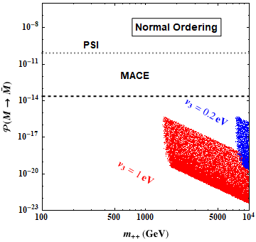
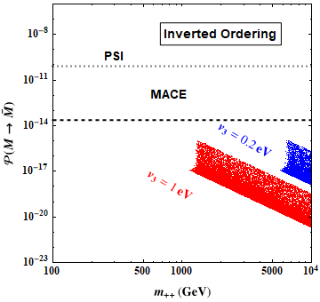
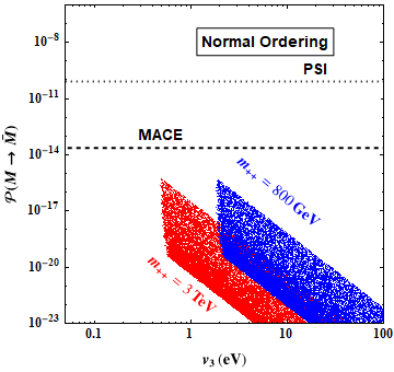
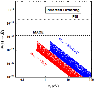
Figure 1: Upper: Scatter plots of the doubly charged Higgs mass $m_{++}$ and the conversion probability $P$ in the type-II seesaw with $v_{3}=0.2$ eV (blue points) and $v_{3}=1$ eV (red points) for Normal Ordering (left) and Inverted Ordering (right). Lower: Scatter plots of the vev $v_{3}$ and the conversion probability $P$ in the type-II seesaw with $m_{++}=800$ GeV (blue points) and $m_{++}=3$ TeV (red points) for Normal Ordering (left) and Inverted Ordering (right). All the plotted points are allowed by the flavor and collider constraints.

In this section, we present our numerical results by sampling in the model parameter space. For simplicity, we assume all the model parameters are real. In our scanning, we selected models that predict the neutrino mass squared differences and mixing angles to be within the experimentally allowed ranges for both normal ordering (NO) and inverted ordering (IO) at $3\sigma$ confidence level obtained from the existing neutrino oscillation data as shown Table II. Although the recently released data from T2K and NO$\nu$A Collaborations prefer a non-zero Dirac $CP$ phase $\delta_{\rm CP}$, this result is still not conclusive. Thus, we still allow $\delta_{\rm CP}$ to be varied within $[0,\,2\pi]$. We also take into account the cosmological limit on the sum of neutrino masses so that the lightest neutrino mass is sampled uniformly within the range of $[0,\,0.05\,{\rm eV}]$. The value of the triplet Higgs VEV is adopted to be from $10^{-2}$ eV to $1$ GeV, while the mass doubly-charged Higgs $\xi^{\pm\pm}$ is allowed to be within $[100\leavevmode\nobreak\ {\rm GeV},\,10\leavevmode\nobreak\ {\rm TeV}]$. Furthermore, we require that the selected models should satisfy the stringent bounds for cLFV processes, such as $\mu\to e\gamma$ and $\mu^{+}\to e^{-}e^{+}e^{+}$. For the remaining model parameters, we compare their predicted muonium-to-antimuonium conversion probability ${\cal P}(M\leftrightarrow\bar{M})$ with the existing PSI bound and the expected MACE sensitivity. In the following, we shall give the final scanning results for the Type-II and hybrid seesaw models, respectively.

V.1 Type II seesaw

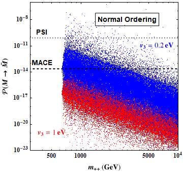
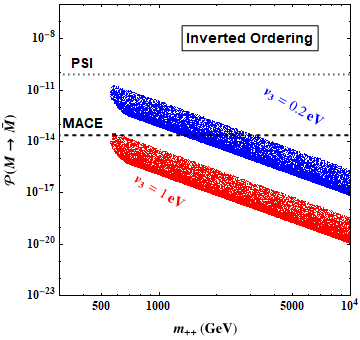
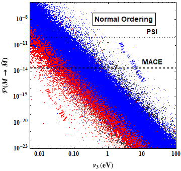
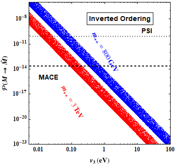
Figure 2: Upper: Scatter plots of the doubly charged Higgs mass $m_{++}$ and the conversion probability $P$ in the hybrid seesaw model with $v_{3}=0.2$ eV (blue points) and $v_{3}=1$ eV (red points) for Normal Ordering (left) and Inverted Ordering (right). Lower: Scatter plots of the vev $v_{3}$ and the conversion probability $P$ in the hybrid seesaw model with $m_{++}=800$ GeV (blue points) and $m_{++}=3$ TeV (red points) for Normal Ordering (left) and Inverted Ordering (right). All the plotted points are allowed by the flavor and collider constraints.

In this case, we assume all of the neutrino mass comes from the triplet Higgs, while the contribution from the right-handed neutrino can be negligible. In Fig. 1 we show the scan result by requiring the neutrino mass satisfying the observation. Since there is an ambiguity in the neutrino mass ordering, we split our analysis in these two cases. The left panels show the preferred parameter space for neutrino mass Normal Ordering and the right panels that of Inverted Ordering. For the top two plots, we fixed the vacuum value of the triplet Higgs at 1 eV (red) and 0.2 eV (blue). We find for $v_{3}=1$ eV, the doubly-charged Higgs should be heavier than around 1.5 TeV to evade the limit from flavor constraints, particularly from $\mu^{+}\rightarrow e^{-}e^{+}e^{+}$. In the case of $v_{3}=0.2$ eV, the limit on the doubly-charged Higgs is stronger since a larger Yukawa coupling is needed to generate the neutrino mass for a smaller vacuum value of $\Delta$. We note that the preferred parameter space behaves as a band due to the uncertainty of the neutrino mass parameter. Finally, we find all the survived parameter space predicts a muonium-antimuonium conversion probability less than $10^{-15}$ which is beyond the reach of the future MACE experiment.

V.2 Hybrid seesaw

As shown in previous model, the strongest limit arises from the cLFV processes, such as $\mu^{+}\to e^{+}\gamma$ and $\mu^{+}\to e^{-}e^{+}e^{+}$. The reason is that from the PMNS matrix we can see the neutrino mixing is relatively large and a large off-diagonal terms in the neutrino mass matrix are needed. Since the neutrino mass matrix mainly originates from the triplet Higgs, it requires a large flavor changing coupling between the triplet Higgs and the leptons, inducing a large flavor changing effect. In the hybrid seesaw model, the flavor constrains could be weaker due to the contribution of off-diagonal terms from right-handed neutrino. Specifically, here we consider that all off-diagonal terms of the neutrino mass matrix originate from the right-handed neutrino, thus all of Yukawa couplings $y_{\nu}$ are fixed. Hence all the flavor constraints could be removed .

The final scanning results are shown in Fig. 2. As before, the upper two scatter plots show the muonium-to-antimuonium conversion probability ${\cal P}(M\leftrightarrow\bar{M})$ as a function of the doubly-charged Higgs mass $m_{++}$ for both NO (left panel) and IO (right panel), while the lower two ones correspond to parameter spaces in ${\cal P}(M\leftrightarrow\bar{M})$ vs. $v_{3}$ plane. Compared with the previous Type-II seesaw case, it is clear that the allowed parameter spaces for the hybrid seesaw model are enlarged greatly, extending aggressively into the low doubly-charged Higgs mass region and the low triplet VEV $v_{3}$ region. Due to the relax of cLFV constraints in this hybrid model, the lower bounds on the doubly-charged Higgs mass for both NO and IO cases around 600 GeV are given by the collider searches for $\xi^{\pm\pm}$. As a result, it is seen that MACE can increase the detection region considerably. Concretely, for $v_{3}=0.2$ eV, MACE can detect doubly-charged Higgs as heavy as 3 TeV. On the other hand, for a fixed $m_{++}$, MACE has an ability to measure the parameter region with $v_{3}<1$ eV for both orderings, which is almost one order more sensitive than the PSI detector. The study in this subsection demonstrates the advantage and the necessity of MACE in the probing and constraining the triplet scalar in the seesaw models.

VI Summary and conclusion

In the present paper, we have discussed prospects of the proposed MACE experiment to search for the muonium-to-antimuonium conversion process in the type-II and hybrid seesaw models, the latter of which is an extension of the type-II seesaw by including a single heavy right-handed neutrino. Note that the leading-order contributions to the $M-\bar{M}$ conversion probability in both models are induced at tree level by the doubly-charged scalar originated in the $SU(2)_{L}$ triplet scalar. Thus, MACE can effectively measure the parameter space related to this triplet scalar. By utilizing the high-quality slow muon sources at CSNS, together with other significant advances in the detector technologies, MACE has been shown to be able to improve the sensitivity to the conversion probability by almost three orders of magnitude compared with the existing PSI experiment accomplished more than 20 years ago. Therefore, a large uncharted model parameter space is expected to be probed by MACE, which is complementary to direct collider searches, neutrino oscillations and other cLFV channels such as $\mu^{+}\to e^{+}\gamma$ and $\mu^{+}\to e^{-}e^{+}e^{+}$. As a result, it is shown that MACE is not sensitive to the parameter space of interest surviving from the collider and flavor limits. On the other hand, for the hybrid seesaw model, MACE can reach unexplored parameter region, and thus provides useful information on the triplet scalar complementary to other cLFV experiments like MEG-II and Mu3e. In other words, if no positive signals are observed by MACE in the future, we shall be able to set a much more stringent upper bound on the mass of the doubly-charged scalar around 1.2 TeV for $v_{3}=1$ eV in the case of Inverted Ordering, which will surpass the corresponding LHC limits even by taking into account the uncertainties involving the neutrino mass ordering or the VEV of the triplet scalar. Even for the NO, the prospect of MACE can reach a doubly-charged Higgs as heavy as 3 TeV for $v_{3}=1$ eV. In summary, with the advent of MACE, the muonium-to-antimuonium conversion will become one of golden channels to study the cLFV physics, which, together with other flavor and collider searches, will shed light on the mystery of the neutrino masses.

Appendix

VI.1 Higgs Potential

We consider the general Higgs potential for a doublet $\Phi=(h^{+},h^{0})^{T}$ and a triplet Higgs $\Delta$ Chun:2003ej .

$$V(\Phi,\Delta)= m^{2}(\Phi^{\dagger}\Phi)+\lambda_{1}(\Phi^{\dagger}\Phi)^{2}+M_{\Delta}^{2}\mathrm{Tr}(\Delta^{\dagger}\Delta)+\lambda_{2}[\mathrm{Tr}(\Delta^{\dagger}\Delta)]^{2}+\lambda_{3}\mathrm{Tr}(\Delta\Delta)\mathrm{Tr}(\Delta^{\dagger}\Delta^{\dagger}),$$ (27)

$$+\lambda_{4}(\Phi^{\dagger}\Phi)[\mathrm{Tr}(\Delta^{\dagger}\Delta)]+\lambda_{5}(\Phi^{\dagger}\Delta^{\dagger}\Delta\Phi)+\lambda_{6}(\Phi^{\dagger}\Delta\Delta^{\dagger}\Phi)+\frac{1}{2}\mu(\Phi^{T}\varepsilon\Delta^{\dagger}\Phi)+\mbox{h.c.}$$

The breaking can be explicit when V($\Phi,\Delta$) is supposed to contain the trilinear L-nonconserving term ($\Phi^{T}\Delta\Phi$). In this case the masses of the new Higgs particles $M_{\Delta}$ in the model can be arbitrary large. Collect the following soft lepton number violating trilinear interaction between $\Delta$ and $\Phi$ from the Higgs potential:

$${\cal L}_{\mathrm{soft}} = -\frac{1}{2}\mu\Phi^{T}\varepsilon\Delta^{\dagger}\Phi+\mbox{h.c.},$$ (28)

$$= -\frac{1}{2}\mu\left[(h^{+})^{2}\xi^{--}-\sqrt{2}h^{+}h^{0}\xi^{-}-(h^{0})^{2}\xi^{0{\dagger}}\right]+\mbox{h.c.}$$

where $\mu$ is an undetermined parameter. The minimum of Higgs potential is presented in the following:

$$V_{\mathrm{min}}(\Phi,\Delta)=\frac{1}{2}m^{2}v_{1}^{2}+M_{\Delta}^{2}v_{3}^{2}+\frac{1}{4}\lambda_{1}v_{1}^{4}+\lambda_{2}v_{3}^{4}+\frac{1}{2}\lambda_{4}v_{1}^{2}v_{3}^{2}+\frac{1}{2}\lambda_{6}v_{1}^{2}v_{3}^{2}+\frac{1}{2}\mu v_{1}^{2}v_{3}$$ (29)

After the spontaneous symmetry breaking (SSB), solving the equation $\frac{\partial V_{\mathrm{min}}(\Phi,\Delta)}{\partial v_{i}}=0$ leads to:

$$\langle h^{0}\rangle=\frac{v_{1}}{\sqrt{2}},\quad\langle\xi^{0}\rangle=v_{3}.$$

$$v_{1}^{2}=-\frac{m^{2}}{\lambda_{1}},\quad v_{3}=-\frac{\mu v_{1}^{2}}{2\left(2M^{2}+v_{1}^{2}\lambda_{4}+v_{1}^{2}\lambda_{6}\right)}$$ (30)

where $\mu<0$, $m^{2}<0$ and $M_{\Delta}^{2}>0$. When $|\mu|$ is small enough compared with the weak scale, the smallness of neutrino masses is attributed to the tiny $\mu$, which is estimated at the eV scale in the case where $y_{N}\sim O(1)$ and $M_{\Delta}\sim v_{1}$. For completeness, the charged Higgs masses are listed below:

$$m_{+} = M_{\Delta}^{2}+\frac{1}{2}(\lambda_{4}+\frac{\lambda_{5}+\lambda_{6}}{2})v_{1}^{2}$$ (31)

$$m_{++} = M_{\Delta}^{2}+\frac{1}{2}(\lambda_{4}+\lambda_{5})v_{1}^{2}$$ (32)

VI.2 Gauge Sector

Now let us move to gauge couplings $D_{\mu}\xi D^{\mu}\xi$. Since there is a triplet scalar, we have to use 3-dimension representation of SU(2) group.

$$T_{1}=\left(\begin{array}[]{lll}0&\frac{1}{\sqrt{2}}&0\\ \frac{1}{\sqrt{2}}&0&\frac{1}{\sqrt{2}}\\ 0&\frac{1}{\sqrt{2}}&0\end{array}\right),\quad T_{2}=\left(\begin{array}[]{lll}0&-\frac{i}{\sqrt{2}}&0\\ \frac{i}{\sqrt{2}}&0&-\frac{i}{\sqrt{2}}\\ 0&\frac{i}{\sqrt{2}}&0\end{array}\right),\quad T_{3}=\left(\begin{array}[]{ccc}1&0&0\\ 0&0&0\\ 0&0&-1\end{array}\right)$$ (33)

$$T^{+}=T^{1}+iT^{2}=\left(\begin{array}[]{ccc}0&\sqrt{2}&0\\ 0&0&\sqrt{2}\\ 0&0&0\end{array}\right),\quad T^{-}=T^{1}-iT^{2}=\left(\begin{array}[]{ccc}0&0&0\\ \sqrt{2}&0&0\\ 0&\sqrt{2}&0\end{array}\right)$$ (34)

$$D_{\mu}\xi=\partial_{\mu}-ig_{1}Y_{\xi}B_{\mu}-ig_{2}A_{\mu}^{a}T^{a}=\left(\begin{array}[]{l}\left(\partial_{\mu}-iB_{\mu}g_{1}-iA^{3}_{\mu}g_{2}\right)\xi^{\text{++}}-ig_{2}W^{+}_{\mu}\xi^{+}\\ \left(\partial_{\mu}-iB_{\mu}g_{1}\right)\xi^{+}-ig_{2}W^{-}_{\mu}\xi^{\text{++}}-ig_{2}W^{+}_{\mu}\xi^{0}\\ \left(\partial_{\mu}-iB_{\mu}g_{1}+iA^{3}_{\mu}g_{2}\right)\xi^{0}-ig_{2}W^{-}_{\mu}\xi^{+}\end{array}\right)$$ (35)

$$W_{\mu}^{\pm} =\frac{1}{\sqrt{2}}(A_{\mu}^{1}\mp iA_{\mu}^{2})$$ (36)

$$s_{w} \equiv\sin\theta_{w}=\frac{g_{1}}{\sqrt{g_{1}^{2}+g_{2}^{2}}}$$

$$c_{w} \equiv\cos\theta_{w}=\frac{g_{2}}{\sqrt{g_{1}^{2}+g_{2}^{2}}}$$

$$A_{\mu}^{3} =Z_{\mu}^{0}\cos\theta_{w}+A_{\mu}\sin\theta_{w}$$

$$B_{\mu} =-Z_{\mu}^{0}\sin\theta_{w}+A_{\mu}\cos\theta_{w}$$

After spontaneous symmetry breaking, $\Delta$ develops a vacuum expectation value. If physical vector bosons are introduced, we have

$$D^{\mu*}(\xi+\langle\xi\rangle)=\left(\begin{array}[]{l}iW^{-\mu}\xi^{-}g_{2}+\left[ig_{2}\left(Z^{\text{0$\mu$}}c_{w}+A^{\mu}s_{w}\right)+ig_{1}\left(A^{\mu}c_{w}-Z^{\text{0$\mu$}}s_{w}\right)+\partial^{\mu}\right]\xi^{--}\\ iA^{\mu}\xi^{-}c_{w}g_{1}+ig_{2}\left(W^{\text{+$\mu$}}\xi^{--}+W^{-\mu}\xi^{\text{0*}}\right)+\left(\partial^{\mu}-iZ^{\text{0$\mu$}}g_{1}s_{w}\right)\xi^{-}\\ iW^{\text{+$\mu$}}\xi^{-}g_{2}+\left[-ig_{2}\left(Z^{\text{0$\mu$}}c_{w}+A^{\mu}s_{w}\right)+ig_{1}\left(A^{\mu}c_{w}-Z^{\text{0$\mu$}}s_{w}\right)+\partial^{\mu}\right]\xi^{\text{0*}}\end{array}\right)$$ (37)

They will contribute to gauge boson masses,

$$\begin{split}|D_{\mu}\langle\xi\rangle|^{2}&=W_{\mu}^{+}W^{-\mu}g_{2}^{2}v_{3}^{2}+Z_{\mu}^{0}Z^{\text{0$\mu$}}\left(c_{w}^{2}g_{2}^{2}+2c_{w}g_{1}s_{w}g_{2}+g_{1}^{2}s_{w}^{2}\right)v_{3}^{2}\\ &\quad+Z_{\mu}^{0}A^{\mu}\left(-g_{1}g_{2}c_{w}^{2}-g_{1}^{2}s_{w}c_{w}+g_{2}^{2}s_{w}c_{w}+g_{1}g_{2}s_{w}^{2}-g_{1}g_{2}c_{w}^{2}-g_{1}^{2}s_{w}c_{w}+g_{2}^{2}s_{w}c_{w}+g_{1}g_{2}s_{w}^{2}\right)v_{3}^{2}\\ &\quad+A_{\mu}A^{\mu}\left(c_{w}^{2}g_{1}^{2}-2c_{w}g_{2}s_{w}g_{1}+g_{2}^{2}s_{w}^{2}\right)v_{3}^{2}\\ &=g_{2}^{2}v_{3}^{2}W^{+\mu}W_{\mu}^{-}+\frac{g_{2}^{2}v_{3}^{2}}{\cos^{2}\theta_{w}}Z^{0\mu}Z_{\mu}^{0}\end{split}$$ (38)

In addition, the traditional SM contains gauge mass terms:

$$\mathcal{L}_{\mathrm{GM}}=\frac{1}{4}g_{2}^{2}v_{1}^{2}W_{\mu}^{+}W^{-\mu}+\frac{1}{8}\frac{g_{2}^{2}v_{1}^{2}}{\cos^{2}\theta_{w}}Z_{\mu}^{0}Z^{0\mu}$$ (39)

which violates the custodial symmetry such as

$$\rho=\frac{M_{W}^{2}}{M_{Z}^{2}\cos^{2}\theta_{w}}=\frac{\frac{1}{4}g_{2}^{2}v_{1}^{2}+g_{2}^{2}v_{3}^{2}}{\frac{1}{4}g_{2}^{2}v_{1}^{2}+2g_{2}^{2}v_{3}}=1-\frac{v_{3}^{2}}{\frac{1}{4}v_{1}^{2}+2v_{3}^{2}}$$ (40)

As $|\mu|$ is small enough so that $v_{3}\ll v_{1}$, $\rho\approx 1$ meets the requirement from electroweak precision experiments whereas detectable lepton flavor violating processes are expected. Since the lepton number is restored for $\mu=0$, it may be natural to have a small $\mu$ as a consequence of a tiny lepton number violation. In fact, there is a tree-level lepton flavor violating process $e^{-}\mu^{+}\longrightarrow e^{+}\mu^{-}$ mediated by $\xi^{++}$ due to the interaction term $\bar{e}^{c}_{i}P_{L}e_{j}\xi^{++}$ Chang:1989uk just as the related term of Eq. (13).

References

- [1] Niklaus Berger. The Mu3e Experiment. Nucl. Phys. B Proc. Suppl., 248-250:35–40, 2014.
- [2] A. M. Baldini et al. The design of the MEG II experiment. Eur. Phys. J. C, 78(5):380, 2018.
- [3] R. Abramishvili et al. COMET Phase-I Technical Design Report. PTEP, 2020(3):033C01, 2020.
- [4] L. Bartoszek et al. Mu2e Technical Design Report. 10 2014.
- [5] B. Pontecorvo. Mesonium and anti-mesonium. Sov. Phys. JETP, 6:429, 1957.
- [6] T. E. Clark and S. T. Love. Muonium - anti-muonium oscillations and massive Majorana neutrinos. Mod. Phys. Lett. A, 19:297–306, 2004.
- [7] Gorazd Cvetic, Claudio O. Dib, C. S. Kim, and J. D. Kim. Muonium-antimuonium conversion in models with heavy neutrinos. Phys. Rev. D, 71:113013, 2005.
- [8] Boyang Liu. Gauge Invariance of the Muonium-Antimuonium Oscillation Time Scale and Limits on Right-Handed Neutrino Masses. Mod. Phys. Lett. A, 24:335–348, 2009.
- [9] Darwin Chang and Wai-Yee Keung. Constraints on Muonium - anti-Muonium Conversion. Phys. Rev. Lett., 62:2583, 1989.
- [10] H. Fujii, Y. Mimura, K. Sasaki, and T. Sasaki. Muonium, hyperfine structure and the decay mu+ — e+ + anti-electron-neutrino + muon-neutrino in models with dilepton gauge baryons. Phys. Rev. D, 49:559–562, 1994.
- [11] Paul H. Frampton and Masayasu Harada. Constraints from precision electroweak data on leptoquarks and bileptons. Phys. Rev. D, 58:095013, 1998.
- [12] A. Halprin and A. Masiero. Muonium - anti-muonium oscillations and exotic muon decay in broken R-parity SUSY models. Phys. Rev. D, 48:2987–2989, 1993.
- [13] Peter Herczeg and Rabindra N. Mohapatra. Muonium to anti-muonium conversion and the decay mu+ — e+ anti-neutrino neutrino in left-right symmetric models. Phys. Rev. Lett., 69:2475–2478, 1992.
- [14] A. Halprin. NEUTRINOLESS DOUBLE BETA DECAY AND MUONIUM - ANTI-MUONIUM TRANSITIONS. Phys. Rev. Lett., 48:1313–1316, 1982.
- [15] Renae Conlin and Alexey A. Petrov. Muonium-antimuonium oscillations in effective field theory. Phys. Rev. D, 102(9):095001, 2020.
- [16] L. Willmann et al. New bounds from searching for muonium to anti-muonium conversion. Phys. Rev. Lett., 82:49–52, 1999.
- [17] Jian Tang et al. Letter of interest contribution to snowmass21. https://www.snowmass21.org/docs/files/summaries/RF/SNOWMASS21-RF5_RF0_Jian_Tang-126.pdf, 2020.
- [18] G. Feinberg and S. Weinberg. Conversion of Muonium into Antimuonium. Phys. Rev., 123:1439–1443, 1961.
- [19] J. Schechter and J. W. F. Valle. Neutrino Masses in SU(2) x U(1) Theories. Phys. Rev. D, 22:2227, 1980.
- [20] Mitsuru Kakizaki and Masahiro Yamaguchi. Singular Kahler potential and heavy top quark in a democratic mass matrix model. Phys. Lett. B, 573:123–130, 2003.
- [21] Ivan Esteban, M. C. Gonzalez-Garcia, Michele Maltoni, Thomas Schwetz, and Albert Zhou. The fate of hints: updated global analysis of three-flavor neutrino oscillations. JHEP, 09:178, 2020.
- [22] R. Primulando, J. Julio, and P. Uttayarat. Scalar phenomenology in type-II seesaw model. JHEP, 08:024, 2019.
- [23] Palash B. Pal. Constraints on a Muon - Neutrino Mass Around 100-kev. Nucl. Phys. B, 227:237–251, 1983.
- [24] G. K. Leontaris, K. Tamvakis, and J. D. Vergados. Lepton and Family Number Violation From Exotic Scalars. Phys. Lett. B, 162:153–159, 1985.
- [25] Morris L. Swartz. Limits on Doubly Charged Higgs Bosons and Lepton Flavor Violation. Phys. Rev. D, 40:1521, 1989.
- [26] R. N. Mohapatra. Rare decays of the tau lepton as a probe of the left-right symmetric theories of weak interactions. Phys. Rev. D, 46:2990–2995, 1992.
- [27] V. Cirigliano, A. Kurylov, M. J. Ramsey-Musolf, and P. Vogel. Lepton flavor violation without supersymmetry. Phys. Rev. D, 70:075007, 2004.
- [28] A. G. Akeroyd, Mayumi Aoki, and Hiroaki Sugiyama. Lepton Flavour Violating Decays tau — anti-l ll and mu — e gamma in the Higgs Triplet Model. Phys. Rev. D, 79:113010, 2009.
- [29] D. N. Dinh, A. Ibarra, E. Molinaro, and S. T. Petcov. The Conversion in Nuclei, Decays and TeV Scale See-Saw Scenarios of Neutrino Mass Generation. JHEP, 08:125, 2012. [Erratum: JHEP 09, 023 (2013)].
- [30] P. S. Bhupal Dev, Michael J. Ramsey-Musolf, and Yongchao Zhang. Doubly-Charged Scalars in the Type-II Seesaw Mechanism: Fundamental Symmetry Tests and High-Energy Searches. Phys. Rev. D, 98(5):055013, 2018.
- [31] Manoel M. Ferreira, Tessio B. de Melo, Sergey Kovalenko, Paulo R. D. Pinheiro, and Farinaldo S. Queiroz. Lepton Flavor Violation and Collider Searches in a Type I + II Seesaw Model. Eur. Phys. J. C, 79(11):955, 2019.
- [32] U. Bellgardt et al. Search for the Decay mu+ — e+ e+ e-. Nucl. Phys. B, 299:1–6, 1988.
- [33] Peter Minkowski. at a Rate of One Out of Muon Decays? Phys. Lett. B, 67:421–428, 1977.
- [34] C. S. Lim and T. Inami. Lepton Flavor Nonconservation and the Mass Generation Mechanism for Neutrinos. Prog. Theor. Phys., 67:1569, 1982.
- [35] Paul Langacker and David London. Lepton Number Violation and Massless Nonorthogonal Neutrinos. Phys. Rev. D, 38:907, 1988.
- [36] W. J. Marciano and A. I. Sanda. Exotic Decays of the Muon and Heavy Leptons in Gauge Theories. Phys. Lett. B, 67:303–305, 1977.
- [37] T. P. Cheng and Ling-Fong Li. in Theories With Dirac and Majorana Neutrino Mass Terms. Phys. Rev. Lett., 45:1908, 1980.
- [38] A. Ilakovac and A. Pilaftsis. Flavor violating charged lepton decays in seesaw-type models. Nucl. Phys. B, 437:491, 1995.
- [39] F. Deppisch and J. W. F. Valle. Enhanced lepton flavor violation in the supersymmetric inverse seesaw model. Phys. Rev. D, 72:036001, 2005.
- [40] Bo He, T. P. Cheng, and Ling-Fong Li. A Less suppressed mu — e gamma loop amplitude and extra dimension theories. Phys. Lett. B, 553:277–283, 2003.
- [41] L. Lavoura. General formulae for f(1) — f(2) gamma. Eur. Phys. J. C, 29:191–195, 2003.
- [42] D. V. Forero, S. Morisi, M. Tortola, and J. W. F. Valle. Lepton flavor violation and non-unitary lepton mixing in low-scale type-I seesaw. JHEP, 09:142, 2011.
- [43] R. Alonso, M. Dhen, M. B. Gavela, and T. Hambye. Muon conversion to electron in nuclei in type-I seesaw models. JHEP, 01:118, 2013.
- [44] A. M. Baldini et al. Search for the lepton flavour violating decay with the full dataset of the MEG experiment. Eur. Phys. J. C, 76(8):434, 2016.
- [45] Joydeep Chakrabortty, H. Zeen Devi, Srubabati Goswami, and Sudhanwa Patra. Neutrinoless double- decay in TeV scale Left-Right symmetric models. JHEP, 08:008, 2012.
- [46] A. Gando et al. Search for Majorana Neutrinos near the Inverted Mass Hierarchy Region with KamLAND-Zen. Phys. Rev. Lett., 117(8):082503, 2016. [Addendum: Phys.Rev.Lett. 117, 109903 (2016)].
- [47] M. Agostini et al. Improved Limit on Neutrinoless Double- Decay of 76Ge from GERDA Phase II. Phys. Rev. Lett., 120(13):132503, 2018.
- [48] Morad Aaboud et al. Search for doubly charged Higgs boson production in multi-lepton final states with the ATLAS detector using proton–proton collisions at . Eur. Phys. J. C, 78(3):199, 2018.
- [49] Eung Jin Chun, Kang Young Lee, and Seong Chan Park. Testing Higgs triplet model and neutrino mass patterns. Phys. Lett. B, 566:142–151, 2003.