Theory and simulation of AC electroosmotic suppression of acoustic streaming
Abstract
Acoustic handling of nanoparticles in resonating acoustofluidic devices is often impeded by the presence of acoustic streaming. For micrometer-sized acoustic chambers, this acoustic streaming is typically driven from the fluid-solid interface by viscous shear-stresses generated by the acoustic actuation. AC electroosmosis is another boundary-driven streaming phenomena routinely used in microfluidic devices for handling of particle suspensions in electrolytes. Here, we study how streaming can be suppressed by combining ultrasound acoustics and AC electroosmosis. Based on a theoretical analysis of the electrokinetic problem, we are able to compute numerically a form of the electrical potential at the fluid-solid interface, which is suitable for suppressing a typical acoustic streaming pattern associated with a standing acoustic half-wave. In the linear regime, we even derive an analytical expression for the electroosmotic slip velocity at the fluid-solid interface, and use this as a guiding principle for developing models in the experimentally more relevant nonlinear regime that occurs at elevated driving voltages. We present simulation results for an acoustofluidic device, showing how implementing a suitable AC electroosmosis results in a suppression of the resulting streaming in the bulk of the device by two orders of magnitude.
I Introduction
Acoustofluidics is a rapidly advancing field of research based on the integration of ultrasound and microfluidics in lab-on-a-chip designs. Acoustic waves are used for label-free and efficient particle handling with high bio-compatibility, and the principle has found many application within biotechnology and health care. Examples include acoustic separation, Petersson2007 ; Manneberg2008 ; Ding2014 trapping, Hammarstrom2012 ; Evander2015 tweezing Collins2016 ; Lim2016 ; Baresch2016 as well as enrichment of cancer cells Augustsson2012 ; Antfolk2015 , and bacteria Antfolk2014 ; Li2017 and size-independent sorting of cells.Augustsson2016
System designs for particle migration by ultrasound, termed acoustophoresis, are typically based on elongated fluid channels with cross section dimensions in the range of 0.1 to 1 mm. The frequency of the acoustic waves in aqueous suspensions with wavelengths comparable to the chamber dimensions is thus in the low MHz range. These ultrasound fields are generated by piezoelectric transducers. Two competing forces of nonlinear origin act on particles suspended in the fluid. One force is the acoustic radiation force induced by acoustic wave-scattering by the particles.King1934 ; Yosioka1955 ; Doinikov1997 ; Settnes2012 ; Karlsen2015 This force focuses particles in nodes or antinodes of the acoustic waves, and it scales with the particle volume.Muller2013 The other force is the viscous Stokes drag due to the acoustic streaming,LordRayleigh1884 ; Schlichting1932 ; Westervelt1953 ; Nyborg1958 which scales linearly with the particle radius and tends to swirl particles around. Because of the different scalings, streaming-induced drag force is the dominating force for particles smaller than a critical size. For an aqueous suspension of spherical polystyrene particles in a 1-MHz ultrasound field, the critical diameter has been determined to be around .Muller2012 ; Barnkob2012a To ease the acoustic manipulation of sub-µm particles, such as bacteria, viruses, and exosomes, we seek to suppress the acoustic streaming.
There are two types of acoustic streaming: The boundary-layer-driven streaming originating from the viscous boundary layers near the fluid-solid interfaces, as first analyzed analytically by Lord Rayleigh LordRayleigh1884 and later studied in more detail,Nyborg1958 ; Lee1989 ; Vanneste2011 ; Bach2018 and the bulk-driven streaming generated by attenuation of acoustic waves in the bulk of the fluid,Eckart1948 an effect that is typically negligible in microfluidics except for rotating acoustic fields.bach2019
Electroosmosis, the steady motion of electrolytic solutions with respect to a charged surface by an external electric potential, is another type of boundary-driven streaming.Squires2004 The principle has been used to create, say, micropumps with no moving parts for lab-on-a-chip systems.Ajdari2000 ; Brown2000 ; Gregersen2007 In particular, AC electroosmotic pumps have gained attention by generating relevant flow velocities at relatively low ac-voltages without electrolysis, thus circumventing the problem of gas formation. Pumping velocities have been reported in the s range,Brown2000 ; Gregersen2007 which is of similar magnitude to typical acoustic streaming velocities.
In this study, we suggest to combine acoustic and AC electroosmotic streaming with a resulting net streaming close to zero. As an example of how to achieve this, we propose a specific design of an electro-acoustic device consisting of a microchannel with surface electrodes for generating electroosmosis, embedded in an elastic solid with an attached piezoelectric transducer for generating acoustics. We emphasize that the analysis is carried out with no intrinsic zeta potential. The ensuing study thus belongs to the body of work, which assumes that the chemically generated intrinsic zeta potential has been removed, say by means of a DC offset in the applied potential or by chemical surface treatments. A thorough study of the effects of an intrinsic zeta potential is left for future work.
The paper is structured as follows: In Section II we present the general theoretical framework. In Section III we consider AC electroosmosis at low excitation voltages, where the electrokinetic problem can be linearized and analytical expressions for the electroosmotic slip velocity are obtained. In Section IV, the analytical solution is compared to full numerical solutions at higher voltages, and we find that the linearized regime capture both qualitative and quantitative behavior at surprisingly high voltages. In Section V, the linearized AC electroosmotic theory is integrated into an existing acoustofluidic simulation adapted from Skov et al.Skov2019 Using an electrode design, which could be produced by standard clean room fabrication techniques, together with an attached piezoelectric transducer, we demonstrate how to obtain heavily suppressed streaming patterns when exciting both AC electroosmosis and ultrasound acoustophoresis. In Section VI, we discuss some of the limitations of the proposed model, and finally we conclude.
II Theory
The core part of the system we analyze is a binary electrolyte in the form of a dilute aqueous suspension of ions, with a single positive ion (subscript ) and a single negative ion (subscript ) of opposite valences . The electrolyte is placed inside a microchannel in the presence of a MHz-ultrasound pressure resonance with angular frequency and an kHz-AC electrical potential with angular frequency . The fundamental continuum fields in the fluid at point and time is the mass density , the pressure , the fluid velocity , and the viscous stress tensor , as well as the concentration fields of the positive and negative ions and , the electrical charge density , and the electric potential . The material parameters of the system are the dynamic viscosity , the bulk viscosity , the speed of sound , the quiescent mass density , the isentropic compressibility , the ionic valence number , the ionic diffusivities and mobilities , as well as the electric permittivity . The governing equations for the fluid including acoustics are the mass continuity and Navier–Stokes equation,
| (1a) | ||||
| (1b) | ||||
| (1c) | ||||
The electrokinetics of the ions are governed by the concentration continuity, Nernst, and Poisson equation,
| (2a) | ||||
| (2b) | ||||
| (2c) | ||||
The fields will be treated in perturbation theory written as
| (3) |
Here, is the unperturbed field, is the first-order acoustic and electric time-harmonic perturbation, and is the unsteady second-order field, which is generated by the inherent nonlinearities in hydrodynamic and electrokinetic equations. The time-averaged second-order response is defined . A time-average of a product of two first-order fields is also a second-order term, written as , where the asterisk denote complex conjugation.
| Parameter | Symbol | Value | Unit |
|---|---|---|---|
| Water properties:Muller2014 | |||
| Mass density | kg | ||
| Compressibility | |||
| Speed of sound | |||
| Shear viscosity | |||
| Bulk viscosity | |||
| Electrolyte permittivityCRC | |||
| Ion properties: | |||
| Average diffusivityCRC | |||
| Valence | - | ||
| Bulk concentration | |||
| Debye length | |||
| Debye frequency | |||
| Pyrex properties:CorningPyrex | |||
| Mass density | |||
| PermittivityCRC | |||
| Longditudinal sound speed | |||
| Transverse sound speed | |||
| Pz26 properties:Ferroperm2017 | |||
| Mass density | |||
| Elastic constants: | |||
| Coupling constants: | |||
| Permittivities: | |||
II.1 Combined acoustics and AC electroosmosis
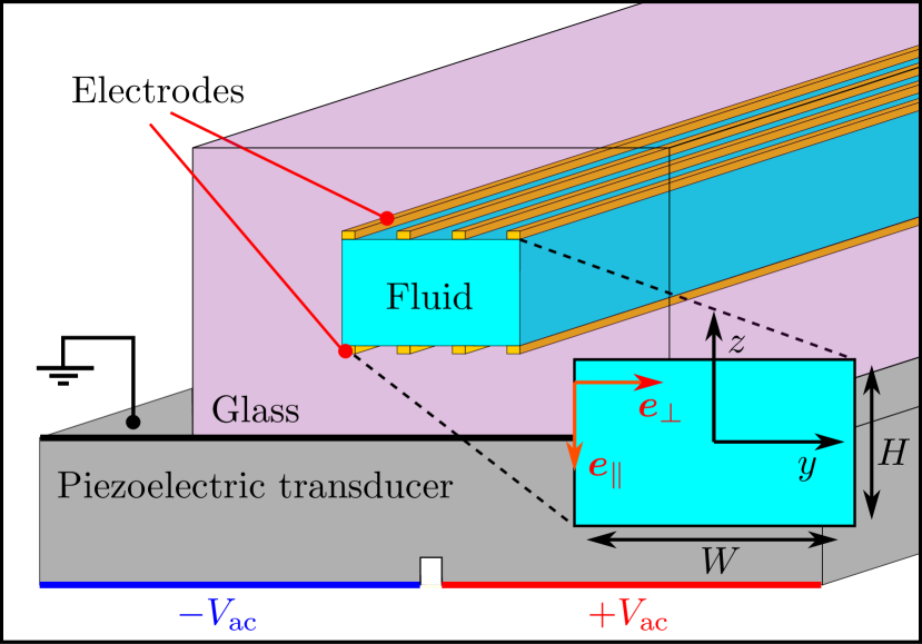
We consider a microfluidic system with integrated acoustics and electroosmosis. A conceptual sketch of such a system is shown in Fig. 1. A piezoelectric transducer actuates the system acoustically and generates acoustic streaming, and electrode arrays surrounding the fluid channel actuate AC electroosmotic streaming, which by proper design aims to counteract and suppress the acoustic streaming. To provide a proof of concept of this streaming suppression, we consider a simple long, straight rectangular fluid channel of dimensions . The acoustic problem in this configuration has previously been studied extensively both theoretically and experimentally,Muller2012 ; Muller2013 ; Muller2014 ; Muller2015 and it is known that the physical properties of the system are well-described by modeling restricted to the two-dimensional (2D) cross section. We thus apply a Cartesian () coordinate system centered in the fluid channel. The equilibrium position of the fluid-solid interface will be denoted , and to describe boundary effects, we apply a local coordinate system at the boundary.
Combining the two phenomena could potentially lead to non-trivial coupled effects. When acoustic waves travel through a ionic suspension, the ions will oscillate slightly out of phase with respect to the solvent. The different mobilities of ionic species will lead to a so-called ionic vibration potential. These potentials normalized by the oscillatory velocity of the fluid are typically of the order of Zana1982 . This effect is around two orders of magnitude lower than what is needed for acoustic streaming suppression by electroosmosis, and it is thus ignored.
As we shall see in the following, AC electroosmotic flows work ideally for , whereas the acoustic actuation frequencies are 1000 times faster in the range of . This separation of time scales allows us to use the acoustomechanical responses at the time-averaged (with respect to ) spatial position of the fluid-solid interface and the oscillating fluid, when computing the electrokinetic responses. Furthermore, the electrokinetic flow is established through the ionic Debye layer at the fluid-solid boundary on the short length scale , whereas the acoustically induced velocity fields are established over a viscous boundary layer of the much longer length scale . Thus, we assume that no significant advection of ions in the Debye layer happen due to the acoustic streaming or vibrational velocity. This spatiotemporal decoupling of the electrokinetics and acoustics is further supported by the fact, that both electroosmotic and acoustic streaming in microchannels are described by linear Stokes flows,Ajdari2000 ; Bach2018 so we conclude that the combined streaming can be derived simply by superimposing the two flows computed separately.
Lastly, as the electric field extends throughout the fluid, dielectrophoretic forces inevitably arise and act on suspended particles.(Voldman2006, ) For most materials in the present context, these forces are several orders of magnitude lower than the acoustic radiation force and the drag forces from streaming. We therefore ignore dielectrophoresis is this analysis.
II.2 Pressure acoustics with viscous boundary layers
To simulate acoustic fields, we follow the approach of Refs. Bach2018, ; Skov2019, . The complex amplitude of the mechanical displacement field in the surrounding solid of the fluid channel and in the piezoelectric transducer is denoted . The complex acoustic pressure field and the associated oscillating fluid velocity field are denoted and , respectively. The steady time-averaged acoustic streaming and the corresponding pressure are then calculated as a Stokes flow with an acoustic slip velocity at the boundary,
| (4a) | ||||
| (4b) | ||||
| (4c) | ||||
In Eq. (4b), the acoustic body force, with the small viscous bulk damping coefficient , is typically negligible for single mode operation in microchannels, bach2019 and the flow is thus mostly driven by the slip velocity . We consider the conventional standing half-wave mode in the acoustic pressure. As we demonstrate later, the acoustic slip velocity for this mode closely resemble that of the classical Rayleigh streaming in fluid channels etched into acoustically hard materials like pyrex glass,
| (5a) | ||||
| (5b) | ||||
where is the average acoustic energy density,
| (6) |
To determine the suppression of streaming numerically, we seek to minimize the average steady streaming in the fluid cross section,
| (7) |
Inspired by Ref. Bach2020, , the streaming suppression is also quantified by the measure,
| (8a) | ||||
| (8b) | ||||
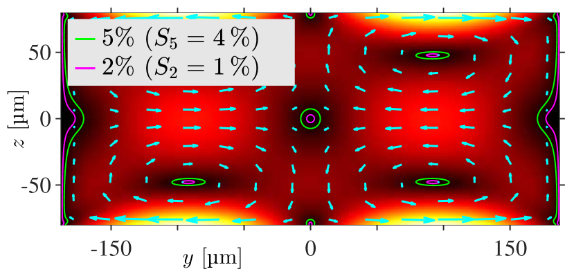
For the initial part of our study, we employ the analytically known acoustic resonance mode derived in Ref. Bach2018, , where the side walls are oscillated as,
| (9) |
Here, is the displacement amplitude, which is tuned to reach a desired average energy density or acoustic streaming. Given the physical parameters used for our study and listed in table Table 1, the resonance frequency for water at is MHz. The acoustic streaming pattern generated by this actuation is shown in Fig. 2.
II.3 AC electroosmosis
We consider an aqueous solution of a simple binary salt, say KCl, with ionic charges , concentrations , diffusivities , and electric mobilities . We also introduce the average diffusivity , which turns out to be the lowest order correction to asymmetric ions in the linearized theory given below. All parameter values are listed in Table 1.
We largely follow the presentations in Refs. Ajdari2000, ; Mortensen2005, but consider a more general externally applied electric potential at the fluid-solid interface,
| (10) |
Here, is some complex-valued function of order unity that describes the shape of the externally applied potential at the boundary, whereas describes its amplitude. We consider flow velocities of sufficiently low amplitudes to describe the fluid as incompressible and drop the nonlinear term in the momentum equation, Eq. (1b). The electric potential is denoted in the fluid and in the surrounding solid and piezoceramic. The full set of governing equations for the electrokinetic problem in the fluid are thus written as,
| (11a) | ||||
| (11b) | ||||
| (11c) | ||||
| (11d) | ||||
The boundary conditions for the electrokinetic problem on electrode surfaces is an equipotential condition and on dielectric surfaces a zero-charge condition. All fluid-solid interfaces admit zero ionic flux normal to the wall (we adopt the notation and ), and the fluid velocity field must fulfill the no slip boundary condition,
| (12a) | |||||
| (12b) | |||||
| (12c) | |||||
| (12d) | |||||
III Linearized analysis of AC electroosmosis
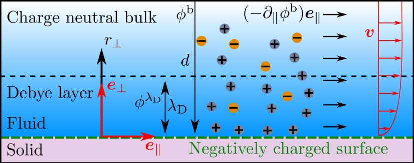
The nonlinear nature of Eq. (11) makes it computationally and analytically challenging to work with general electrokinetic problems. For most computations we opt to use a linearized theory, which heavily reduces the computational footprint. In Section IV we address the error introduced by using this theory at higher voltages. A conceptual sketch of electroosmotic flow generation is shown in Fig. 3. The general idea is to generate an electric charge density at electrode surfaces and then inducing a boundary-driven flow by dragging the ions along the surface with a parallel electric field.
III.1 Linearized electrokinetic equations
We consider the special case where such that , because of the Einstein relation,
| (13) |
where is the Boltzmann constant, is the temperature, and mV is the thermal voltage. Following the treatment in Ref. Mortensen2005, , we consider a zero intrinsic zeta potential and the linearized dynamical Debye–Hückel regime, which is obtained for weak externally applied potentials at the electrode surfaces. Here, the applied potential and the corresponding changes in ionic densities act as first-order fields. Through the non-linear electric body force, this will generate steady streaming as well as double-harmonic streaming with frequency , similar to perturbative acoustic calculations. Denoting the initial ionic concentration by , we write,
| (14a) | ||||
| (14b) | ||||
The second-order electric field and ionic concentrations are omitted, as they do not affect the electroosmotic streaming. We then apply the linearization , and in Eq. (11b), where the latter is valid in the diffusive limit, where ionic advection becomes insignificant compared to diffusion. The first-order electrodynamic fields and the steady time-averaged second-order flow are thus obtained from,Mortensen2005
| (15a) | ||||
| (15b) | ||||
| (15c) | ||||
| (15d) | ||||
where we have introduced the notation
| (16) |
Correspondingly, the boundary condition (12d) becomes,
| (17) |
III.2 Effective AC electrokinetic theory
The rectangular cross section of Fig. 2 only contains planar fluid-solid interfaces, and the potential-shape function of Eq. (10) is assumed to vary on length scales comparable to the chamber dimensions , where . Further, we assume that , which is the relevant limit for our purpose. When an external potential is applied at the fluid-solid interface, ions will accumulate at the wall in a thin layer of length scale . This ionic layer will completely screen off the wall potential for DC wall potentials, but for AC potentials the screening is only partial. Because , we have in Eq. (15a). The perpendicular coordinate away from the surface is called , and thus
| (18) |
where is a constant. The solution for will contain a particular solution , which reflects the partial ionic screening in the thin Debye layer near the boundary, and a homogeneous solution that extends into the bulk,
| (19) |
Combining Eqs. (15b) and (18) and inserting , the two terms in Eq. (19) obey,
| (20a) | ||||
| (20b) | ||||
Using boundary conditions (12a) and (17) with Eqs. (18), (19), and (20a) inserted at , we eliminate to find
| (21a) | ||||
| (21b) | ||||
| (21c) | ||||
For dielectric surfaces , the boundary condition (12b) can similarly be rewritten in terms of ,
| (22) |
The known forms of and can be inserted in Eq. (15d) alongside the calculated . With this, one can compute the steady time-averaged streaming to lowest order in and as a simple Stokes flow with an electroosmotic slip velocity given by as,
| (23a) | ||||
| (23b) | ||||
| (23c) | ||||
| (23d) | ||||
This form of the slip velocity is essentially identical to the one given in Eq. (2) of Ref. Ajdari2000, .
III.3 The analytic electrokinetic double mode
To generate an AC electroosmotic slip velocity opposite to the acoustic Rayleigh slip velocity (5), we use an analytical model in the linearized regime as guidance. We consider an idealized case, where a perfectly smooth potential is generated at the fluid boundary, corresponding to the limit of implementing infinitely many infinitely thin electrodes in our electrode arrays. The more realistic case of a finite amount of electrodes is subsequently assessed in Section V.
In an experimental setup, see Fig. 1, it would likely be desirable to only implement electrodes at the top and bottom boundaries of the microchannel and thus assume a zero-charge conditions at the side walls . The electric potential in the surrounding solid originate from the same electrodes that generate the fluid potential, which leads to . Because most relevant materials for creating microfluidic channels have , Eq. (22) dictates at a dielectric boundary.
A single sinusoidal mode in the electric potential is studied in Ref. Mortensen2005, and shown to give a negligible steady streaming component. Since for , it is clear from Eq. (23d) that a phase difference is needed between the perpendicular- and the parallel component of the electric bulk field at the boundary to generate a significant steady streaming . This is not possible with a single mode, so instead we combine two sinusoidal modes with a relative phase difference ,
| (24a) | ||||
| (24b) | ||||
| (24c) | ||||
We use that , and derive the analytical solution of Eqs. (20b) and (21a) for the bulk potential ,
| (25a) | ||||
| (25b) | ||||
Inserting this in Eq. (23d) leads to an expression for the electroosmotic slip velocity , which depends on both and . We are interested in generating large streaming amplitudes at low applied voltages. The phase difference that leads to the largest streaming amplitude is denoted , and the optimized angular frequency at is denoted . These can both be found analytically and result in the electroosmotic slip velocity,
| (26a) | ||||
| (26b) | ||||
| (26c) | ||||
The optimal phase difference and the corresponding optimal angular frequency are given by,
| (27a) | ||||
| (27b) | ||||
| (27c) | ||||
The slip velocity in Eq. (26) approaches the desired acoustic slip velocity of Eq. (5a) for large values of . Even for , the term will dominate for . The streaming amplitude is seen to increase linearly with for large values of . This continuous growth is caused by the increase in the transverse electrical bulk field generated by the sinusoidal modes for a given surface potential amplitude. In Fig. 4 is shown an electrokinetic simulation with the boundary conditions (24) and , superimposed on the acoustics simulation of Fig. 2. The resulting suppressed streaming is shown next to the separate streaming patterns. For an average acoustic energy density of Pa, the streaming is optimally suppressed through the electroosmotic mode discussed above at mV. We see that the streaming is suppressed below of the Rayleigh streaming amplitude everywhere in the channel, and almost the entire streaming pattern is suppressed below . This result constitutes our first proof of concept of suppression of acoustic streaming by electroosmotic streaming.
Let us discuss the assumptions. It takes very high values of to violate the assumption , and using high order sinusoidal modes could be a valid strategy for creating powerful streaming. However, generating high order sinusoidal modes with discrete electrode arrays would require many electrodes, and in practice it may be desirable to use low order modes. For , we find nm/s for mV. Extrapolating to higher voltages, one would need around mV to reach typical acoustic streaming velocities of around /s. This obviously violates the assumption of , but still remains well below the steric regime.Bazant2007
The efficiency of the electric double-mode potential stems from a phase-matching between the charge density generated by one mode and the electric field of the other mode, which drags the established charge density along the top and bottom surfaces of the channel.
Lastly, we note that the suggested mode combination is not the only way of generating the desired streaming pattern. A combination between a sinusoidal and a linear mode with dielectric side-walls also generate a useful streaming pattern, albeit the analytical solution becomes more complicated. If one controls the potential on the side walls, it also becomes possible to generate clean sinusoidal modes with an even number of half-waves. These possibilities are not explored in this study.
IV Non-linear electroosmotic flows
To reach experimentally relevant streaming velocities, one needs to apply voltages around , well into the nonlinear regime of the electrokinetic problem. In the following, we evaluate the capability of the linearized theory of AC electrokinetics to predict qualitative trends for higher voltages. We adopt a numerical approach inspired by Muller et al.Muller2015 to compare the linear predictions to the full nonlinear system of Eq. (11). For lower voltages, where the linearized theory is valid, we assume the streaming velocity and corresponding pressure to be of the form, Muller2015
| (28) |
where the time dependencies in and describe a transient period. For higher voltages, a more general time dependency could arise by significant mixing of Fourier components through the nonlinear terms in Eqs. (11b) and (11d). Using a fifth-order Romberg integration scheme,Muller2015 ; Press2002 the time-averaged response at a given time is computed numerically as,
| (29) |
IV.1 Numerical implementation
The governing equations (11) are solved with the commercial finite element software COMSOL Multiphysics.Comsol54 Solving the full time-dependent nonlinear equations increases the computational footprint significantly compared to the linearized treatment.
We simulate the transient leading to the time-harmonic problem discussed in the linearized scheme above. The boundary condition (24b) is used directly as formulated in Eqs. (10) and (12a). The boundary condition for the side-walls in Eq. (24a) is replaced by,
| (30) |
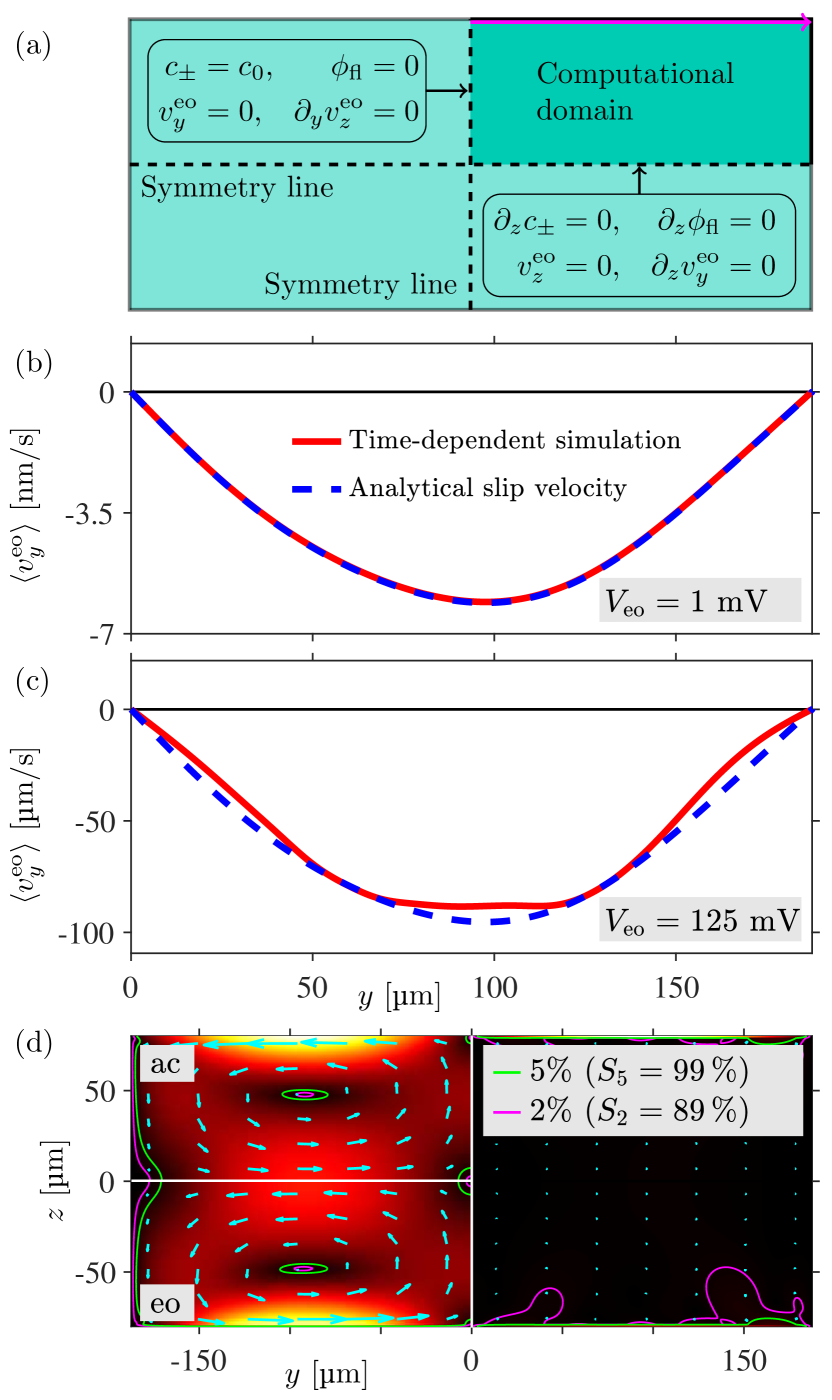
The two central symmetry lines and were used to reduce the computational domain by a factor of four. This is illustrated in Fig. 5(a) alongside the corresponding symmetry boundary conditions. A structured mesh with high resolution near the domain boundaries was used to fully resolve the thin Debye layer, which now has to be taken into account numerically.
As in Ref. Muller2015, , a time-dependent solver is employed with the Generalized alpha time-stepping scheme, where the alpha factor is set to 0.5. A constant time-stepping of was used for all simulations. For simulations with mV, the system Jacobian was set to update at every time-step to stabilize the solutions. The amplitude of the external voltage was gradually ramped up through the first oscillation period as,
| (31) |
The time-dependent solver was run for four electric periods, , and as the physical system is not resonant, a steady state was reached already for . Here, we present two different simulations, one linear with and the other nonlinear with . The time-averaged solution of the latter, which took eight days to finish, turned out to contain higher-than-second-order harmonics with a relative amplitude of about 1 %, signalling the onset of the strongly nonlinear regime. However, due to their relatively low amplitude, these are not discussed further.
IV.2 Results of time-dependent simulations
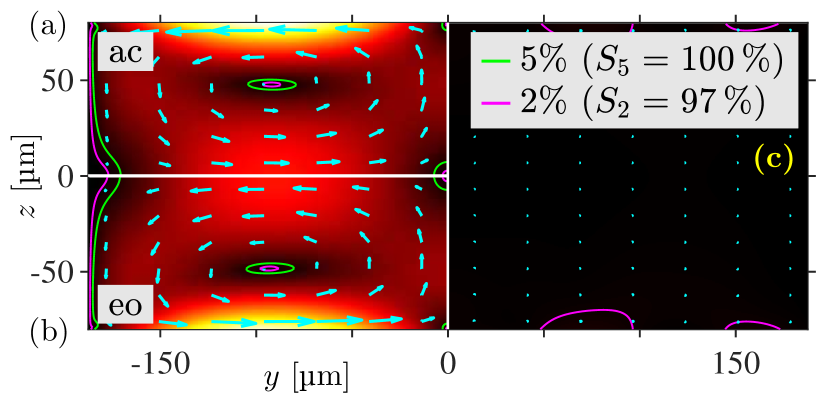
The simulation at mV was primarily made to check the numerical setup. In Fig. 5(b), the time-averaged horizontal velocity component at is shown along the top right boundary, marked by the magenta arrow in Fig. 5(a). Specifically, the field is shown just outside the Debye layer at coordinates , and the comparison with the analytical expression (26b) for the linearized slip velocity shows an almost perfect agreement.
A similar plot is made for mV in Fig. 5(c), and there a notable difference between the two theories appears. The peak amplitude of the time-dependent simulation is s, whereas the linearized theory predicts s, 8% higher. We however notice, that clear quantitative and even decent qualitative features remain. To validate the numerical result of this more nonlinear simulation, the first half period was simulated for increasing mesh refinement, which yielded no significant changes to the solution of the individual time-steps.
Finally, in Fig. 5(d) the time-averaged nonlinear electroosmotic flow at mV is superposed with the idealized acoustic streaming at Pa, in a case chosen to minimize the resulting streaming . As for the linear case Fig. 4(c), the nonlinear streaming in Fig. 5(d) is seen to be heavily suppressed. However here, in contrast to the linearized streaming, small patches of streaming extend from the boundary, where the time-dependent solution is seen to differ the most from the linearized theory. Nevertheless, the streaming is less than 2% of the Rayleigh value in 89% of the domain.
This brief study of electroosmotic streaming in the moderately nonlinear regime suggests that the linearized theory captures the main features of the streaming to a satisfactory degree at the suggested voltage range from 0 to for the initial study presented in this work. We therefore return to the computationally much simpler linearized model in the next section, where we extend our model to include the elastic channel walls, a small number of surface electrodes, and the piezoelectric transducer.
V Numerical 2D device simulations
As sketched in Fig. 1, a typical acoustophoretic device contains a microchannel embedded in an elastic solid which is glued onto a piezoelectric transducer. Consequently, the acoustic response including the streaming is degraded compared to the ideal hard-wall system studied above. Moreover, it is not possible in a real electroosmotic device to create and control a given continuous shape of the surface potential, and instead only a limited number of finite-sized electrodes may be fabricated. In the following, we study through 2D numerical simulations, using the linearized electrokinetic model, to which extend the introduction of these more realistic aspects of the model will diminish the ability to suppress the acoustic streaming by electroosmotic streaming.
V.1 The design of the 2D device
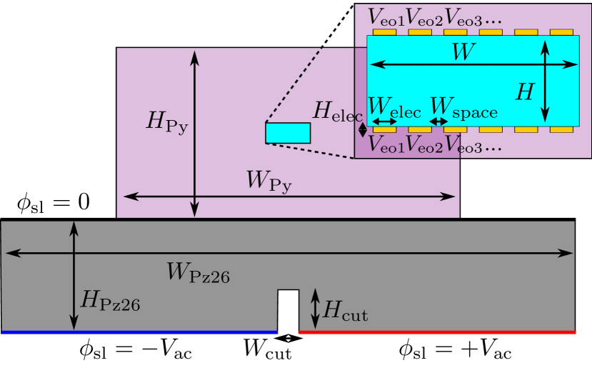
We consider the 2D model sketched in Fig. 6. It contains a microchannel of dimensions filled with a dilute aqueous solution of KCl ions and embedded in an elastic block of pyrex glass of dimensions . The electroosmotic streaming is actuated by voltages on the arrays of rectangular electrodes of dimensions ( and varied) and spacings of dimension engraved into the top and bottom fluid-solid interfaces. The acoustic streaming is actuated by the attached piezoelectric transducer of dimensions modeled as the piezoelectric material Pz26 driven by the potential . A central cut of dimensions is made in the bottom of the transducer to enable antisymmetric actuation.Bode2020
To avoid excessive meshing in the numerical model near the electrodes at the fluid-solid interface, their thickness was chosen to be , which is about 40 times larger than standard clean-room-deposited electrodes typically having a thickness of . Since these enhanced electrodes still comprise a small fraction of the glass volume, they have a negligible effect on the resulting acoustic resonance properties of the channel. Acoustically the electrodes are part of the elastic solid, and electrically, they are modeled as ideal conductors having equipotential surfaces with the applied voltages , respectively, where is applied to the outermost left electrodes at the top and bottom surfaces. The electrode- and spacing widths are always chosen such that with . The -coordinates of the electrode centers for and the potential applied to the electrode arrays, a discretized version of the potential shape (24b) for , are then given by
| (32a) | ||||
| (32b) | ||||
The optimized parameters and are used in all simulations. The side walls and electrode spacings will have a pyrex/water interface with the boundary condition described by Eq. (22).
The system is actuated acoustically by potentials applied to the top and bottom boundaries of the piezoelectric transducer at a numerically determined resonance frequency . A voltage difference of is applied between the two bottom electrodes on the transducer, while the top electrode is grounded. is chosen to reach an average acoustic energy density of Pa.
V.2 Simulation results for the 2D device
In the following, we simulate the combined acoustic and electroosmotic streaming as the Stokes flow (4) with its acoustic body force and acoustic slip, but now also adding the electrokinetics (20b) including the electroosmotic slip velocity (23d),
| (33a) | ||||
| (33b) | ||||
| (33c) | ||||
| (33d) | ||||
| (33e) | ||||
One could worry about using the electroosmotic slip velocity for discrete electrodes, where the edges of these equipotential surfaces introduce length scales that violate the assumptions necessary to derive Eq. (21a) and Eq. (23d). A two-dimensional Debye layer forms at the electrode edges, when the linearized system of equations Eq. (15) is solved with boundary conditions Eq. (12a) and Eq. (17) and a fully resolved boundary layer. This error only occurs at a relatively small part of the computational domain as long as . It was checked numerically, that the implementation of the effective boundary conditions only lead to a relative error of in the streaming pattern for a simple simulation with only two electrodes of widths .
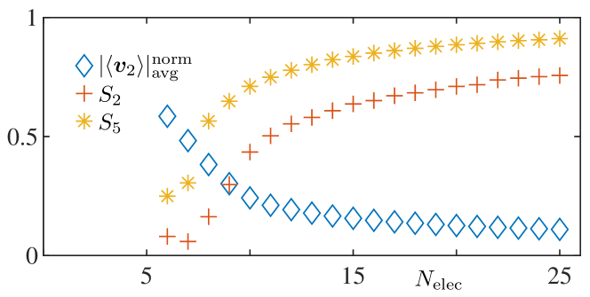
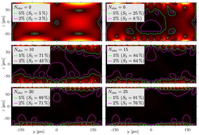
The 2D device simulation was performed for an increasing number of electrodes ranging from with to with . For each value of , the voltage was changed to minimize streaming at Pa. This in turn required a decreasing amplitude for the applied voltage from mV at to mV at . Unsurprisingly, it requires a higher voltage to generate streaming through the discrete electrode pattern compared to the idealized mode.
In Fig. 7 we plot the quantitative measures of the obtained streaming suppression versus the number of electrodes in the arrays. Notably, the initial increase from to electrodes yield the largest increase in the suppression measures, after which a gradual saturation sets in. This suggests that one can look for a reasonable trade off between having many electrodes and reaching a high suppression.
The simulated suppressed streaming is shown in Fig. 8 for 6, 10, 15, 20 and 25. We notice, that the acoustic streaming at is almost identical to the idealized mode in Fig. 2. For the entire central part of the acoustophoretic channel is cleared for streaming amplitudes above of . At , a similar result is seen for the contour lines. Further increases in the electrode count largely just brings the contour lines closer to the boundaries. It is likely undesirable to perform particle focusing close to the boundaries regardless, as this brings adhesion effects into the problem, so increasing the number of electrodes beyond a certain point appears redundant. Right at the boundaries, high streaming velocities are still seen, but these decay on the length scale of the electrode widths. This is expected from the classical Rayleigh solutions, that finds an exponential decay in boundary driven streaming with a characteristic length scale identical to the parallel variations in the slip velocity.LordRayleigh1884
VI Discussion and conclusion
We have already addressed many of the technicalities associated with the method of combining acoustic and electroosmotic streaming. Here, before concluding, we will briefly address two critical points which were neglected in the preceding analysis. First, our analysis of electroosmotic streaming was based on the assumption of a vanishing intrinsic zeta potential. However, the presence of chemically generated charge on relevant interfaces like water/glass is inevitable. Typical values of the zeta potential for borosilicate glass is of the order of mV, Kirby2004 comparable in amplitude to the applied potentials. It is unclear whether or not a DC-offset of this intrinsic wall potential at the discrete electrode arrays would fully nullify its presence, as chemical charges would still form a significant charge cloud in the gaps between electrodes. One idea could be to make these gaps as small as possible.
The intrinsic zeta potential is typically modeled as a constant surface potential, and in the framework of the linearized theory, this would act as a zeroth order field, yielding non-zero gradients in and generating a corresponding initial steady electric equilibrium potential . As noted in Ref. Olesen2006b, , the presence of these extra fields will lower the acquired slip-velocity. A supplemental numerical study in the linearized regime by the authors suggest, that the inclusion of a relatively high intrinsic zeta potential of mV almost halves the slip velocity of the solution used in this paper with the shape remaining the same.
Secondly, we only worked with two-dimensional systems in our present study. While the electroosmotic problem could in principle be implemented invariant along the channel, we know from previous experimental studies,Augustsson2011 that even long, straight microchannel with rectangular cross sections exhibits axial inhomogeneities in the acoustic fields, which renders a 3D analysis necessary for complete characterization of the system. Such a break in the 2D symmetry may yield areas of non-suppressed streaming, which could compromise the performance of the suggested chip design.
In conclusion, we have presented the theoretical framework for a method to effectively suppress acoustic streaming by superposing electroosmotic streaming. We have suggested a specific set of boundary conditions that achieves this suppression in a typical microchannel with a resonant standing half-wave. This idealized electroosmotic mode was then tested in an idealized hard-walled model of the microchannel, in a more realistic model including the transducer, the elastic solid and the microchannel, and for applied voltages in both the linear and nonlinear regime.
Furthermore, we have demonstrated that the electroosmotic streaming pattern derived from a linearized theory largely hold true for relevant amplitudes of applied voltages. Lastly, we also evaluated numerically the capability for suppressing streaming of a specific acoustophoretic chip, where integrated discrete electrodes for generating electroosmosis were implemented. We hope that this theoretical work will inspire the acoustofluidic community to investigate experimentally the possibility of suppressing acoustic streaming in a controlled manner by electroosmosis.
References
- (1) F. Petersson, L. Åberg, A. M. Swärd-Nilsson, and T. Laurell, “Free flow acoustophoresis: microfluidic-based mode of particle and cell separation,” Anal. Chem. 79(14), 5117–23 (2007) \dodoi10.1021/ac070444e.
- (2) O. Manneberg, B. Vanherberghen, J. Svennebring, H. M. Hertz, B. Önfelt, and M. Wiklund, “A three-dimensional ultrasonic cage for characterization of individual cells,” Appl Phys Lett 93(6), 063901–3 (2008) \dodoi10.1063/1.2971030.
- (3) X. Ding, Z. Peng, S.-C. S. Lin, M. Geri, S. Li, P. Li, Y. Chen, M. Dao, S. Suresh, and T. J. Huang, “Cell separation using tilted-angle standing surface acoustic waves,” Proc. Natl. Acad. Sci. U.S.A. 111(36), 12992–12997 (2014) \dodoi10.1073/pnas.1413325111.
- (4) B. Hammarström, T. Laurell, and J. Nilsson, “Seed particle enabled acoustic trapping of bacteria and nanoparticles in continuous flow systems,” Lab Chip 12, 4296–4304 (2012) \dodoi10.1039/C2LC40697G.
- (5) M. Evander, O. Gidlof, B. Olde, D. Erlinge, and T. Laurell, “Non-contact acoustic capture of microparticles from small plasma volumes,” Lab Chip 15, 2588–2596 (2015) \dodoi10.1039/C5LC00290G.
- (6) D. J. Collins, C. Devendran, Z. Ma, J. W. Ng, A. Neild, and Y. Ai, “Acoustic tweezers via sub-time-of-flight regime surface acoustic waves,” Science Advances 2(7), e1600089 (2016) \dodoi10.1126/sciadv.1600089.
- (7) H. G. Lim, Y. Li, M.-Y. Lin, C. Yoon, C. Lee, H. Jung, R. H. Chow, and K. K. Shung, “Calibration of trapping force on cell-size objects from ultrahigh-frequency single-beam acoustic tweezer,” IEEE IEEE T. Ultrason. Ferr. 63(11), 1988–1995 (2016) \dodoi10.1109/TUFFC.2016.2600748.
- (8) D. Baresch, J.-L. Thomas, and R. Marchiano, “Observation of a single-beam gradient force acoustical trap for elastic particles: Acoustical tweezers,” Phys. Rev. Lett. 116, 024301 (2016) \dodoi10.1103/PhysRevLett.116.024301.
- (9) P. Augustsson, C. Magnusson, M. Nordin, H. Lilja, and T. Laurell, “Microfluidic, label-free enrichment of prostate cancer cells in blood based on acoustophoresis,” Anal. Chem. 84(18), 7954–7962 (2012) \dodoi10.1021/ac301723s.
- (10) M. Antfolk, C. Magnusson, P. Augustsson, H. Lilja, and T. Laurell, “Acoustofluidic, label-free separation and simultaneous concentration of rare tumor cells from white blood cells,” Anal. Chem. 87(18), 9322–9328 (2015) \dodoi10.1021/acs.analchem.5b02023.
- (11) M. Antfolk, P. B. Muller, P. Augustsson, H. Bruus, and T. Laurell, “Focusing of sub-micrometer particles and bacteria enabled by two-dimensional acoustophoresis,” Lab Chip 14, 2791–2799 (2014) \dodoi10.1039/c4lc00202d.
- (12) S. Li, F. Ma, H. Bachman, C. E. Cameron, X. Zeng, and T. J. Huang, “Acoustofluidic bacteria separation,” J. Micromech. Microeng. 27(1), 015031 (2017) \dodoi10.1088/1361-6439/27/1/015031.
- (13) P. Augustsson, J. T. Karlsen, H.-W. Su, H. Bruus, and J. Voldman, “Iso-acoustic focusing of cells for size-insensitive acousto-mechanical phenotyping,” Nat. Commun. 7, 11556 (2016) \dodoi10.1038/ncomms11556.
- (14) L. V. King, “On the acoustic radiation pressure on spheres,” Proc. R. Soc. London, Ser. A 147(861), 212–240 (1934) \dodoi10.1098/rspa.1934.0215.
- (15) K. Yosioka and Y. Kawasima, “Acoustic radiation pressure on a compressible sphere,” Acustica 5, 167–173 (1955).
- (16) A. A. Doinikov, “Acoustic radiation force on a spherical particle in a viscous heat-conducting fluid .1. general formula,” J. Acoust. Soc. Am. 101(2), 713–721 (1997) \dodoi10.1121/1.418035.
- (17) M. Settnes and H. Bruus, “Forces acting on a small particle in an acoustical field in a viscous fluid,” Phys. Rev. E 85, 016327 (2012) \dodoi10.1103/PhysRevE.85.016327.
- (18) J. T. Karlsen and H. Bruus, “Forces acting on a small particle in an acoustical field in a thermoviscous fluid,” Phys. Rev. E 92, 043010 (2015) \dodoi10.1103/PhysRevE.92.043010.
- (19) P. B. Muller, M. Rossi, A. G. Marin, R. Barnkob, P. Augustsson, T. Laurell, C. J. Kähler, and H. Bruus, “Ultrasound-induced acoustophoretic motion of microparticles in three dimensions,” Phys. Rev. E 88(2), 023006 (2013) \dodoi10.1103/PhysRevE.88.023006.
- (20) Lord Rayleigh, “On the circulation of air observed in Kundt’s tubes, and on some allied acoustical problems,” Philos. Trans. R. Soc. London 175, 1–21 (1884) \dodoi10.1098/rstl.1884.0002.
- (21) H. Schlichting, “Berechnung ebener periodischer Grenzeschichtströmungen,” Phys. Z. 33, 327–335 (1932).
- (22) P. Westervelt, “The theory of steady rotational flow generated by a sound field,” J. Acoust. Soc. Am. 25(1), 60–67 (1953) \dodoi10.1121/1.1907009.
- (23) W. L. Nyborg, “Acoustic streaming near a boundary,” J. Acoust. Soc. Am. 30(4), 329–339 (1958) \dodoi10.1121/1.1909587.
- (24) P. B. Muller, R. Barnkob, M. J. H. Jensen, and H. Bruus, “A numerical study of microparticle acoustophoresis driven by acoustic radiation forces and streaming-induced drag forces,” Lab Chip 12, 4617–4627 (2012) \dodoi10.1039/C2LC40612H.
- (25) R. Barnkob, P. Augustsson, T. Laurell, and H. Bruus, “Acoustic radiation- and streaming-induced microparticle velocities determined by microparticle image velocimetry in an ultrasound symmetry plane,” Phys. Rev. E 86, 056307 (2012) \dodoi10.1103/PhysRevE.86.056307.
- (26) C. Lee and T. Wang, “Near-boundary streaming around a small sphere due to 2 orthogonal standing waves,” J. Acoust. Soc. Am. 85(3), 1081–1088 (1989) \dodoi10.1121/1.397491.
- (27) J. Vanneste and O. Bühler, “Streaming by leaky surface acoustic waves,” Proc. R. Soc. A 467(2130), 1779–1800 (2011) \dodoi10.1098/rspa.2010.0457.
- (28) J. S. Bach and H. Bruus, “Theory of pressure acoustics with viscous boundary layers and streaming in curved elastic cavities,” J. Acoust. Soc. Am. 144, 766–784 (2018) \dodoi10.1121/1.5049579.
- (29) C. Eckart, “Vortices and streams caused by sound waves,” Phys. Rev. 73, 68–76 (1948) \dodoi10.1103/PhysRev.73.68.
- (30) J. S. Bach and H. Bruus, “Bulk-driven acoustic streaming at resonance in closed microcavities,” Phys. Rev. E 100, 023104 (2019) \dodoi10.1103/PhysRevE.100.023104.
- (31) T. M. Squires and M. Z. Bazant, “Induced-Charge Electro-Osmosis,” J. Fluid Mech. 509(-1), 217–252 (2004) \dodoi10.1017/S0022112004009309.
- (32) A. Ajdari, “Pumping liquids using asymmetric electrode arrays,” Phys Rev E 61(1), 45–48 (2000) \dodoi10.1103/PhysRevE.61.R45.
- (33) A. B. D. Brown, C. G. Smith, and A. R. Rennie, “Pumping of water with ac electric fields applied to asymmetric pairs of microelectrodes,” Phys Rev E 63(1), 016305 (2000) \dodoi10.1103/PhysRevE.63.016305.
- (34) M. M. Gregersen, L. H. Olesen, A. Brask, M. F. Hansen, and H. Bruus, “Flow reversal at low voltage and low frequency in a microfabricated ac electrokinetic pump,” Phys Rev E 76(5), 056305 (2007) \dodoi10.1103/PhysRevE.76.056305.
- (35) N. R. Skov, J. S. Bach, B. G. Winckelmann, and H. Bruus, “3D modeling of acoustofluidics in a liquid-filled cavity including streaming, viscous boundary layers, surrounding solids, and a piezoelectric transducer,” AIMS Mathematics 4, 99–111 (2019) \dodoi10.3934/Math.2019.1.99.
- (36) P. B. Muller and H. Bruus, “Numerical study of thermoviscous effects in ultrasound-induced acoustic streaming in microchannels,” Phys. Rev. E 90(4), 043016 (2014) \dodoi10.1103/PhysRevE.90.043016.
- (37) W. M. Haynes, ed., CRC Handbook of Chemistry and Physics, 97 ed. (CRC Press, Boca Raton, FL, 2016).
- (38) CORNING, Houghton Park C-8, Corning, NY 14831, USA, Glass Silicon Constraint Substrates, http://www.valleydesign.com/Datasheets/Corning%20Pyrex%207740.pdf, accessed 28 November 2019.
- (39) Meggitt A/S, Porthusvej 4, DK-3490 Kvistgaard, Denmark, Ferroperm Matdat 2017, https://www.meggittferroperm.com/materials/, accessed 28 Januar 2021.
- (40) P. B. Muller and H. Bruus, “Theoretical study of time-dependent, ultrasound-induced acoustic streaming in microchannels,” Phys. Rev. E 92, 063018 (2015) \dodoi10.1103/PhysRevE.92.063018.
- (41) R. Zana and E. B. Yeager, “Ultrasonic vibration potentials,” in Modern Aspects of Electrochemistry: No. 14, edited by J. O. Bockris, B. E. Conway, and R. E. White (Springer US, Boston, MA, 1982), pp. 1–60, \dodoi10.1007/978-1-4615-7458-3_1.
- (42) J. Voldman, “Electrical forces for microscale cell manipulation,” Annual Review of Biomedical Engineering 8(1), 425–454 (2006) \dodoi10.1146/annurev.bioeng.8.061505.095739.
- (43) J. S. Bach and H. Bruus, “Suppression of acoustic streaming in shape-optimized channels,” Phys. Rev. Lett. 124, 214501 (2020) \dodoi10.1103/PhysRevLett.124.214501.
- (44) N. Mortensen, L. Olesen, L. Belmon, and H. Bruus, “Electrohydrodynamics of binary electrolytes driven by modulated surface potentials,” Physical review. E, Statistical, nonlinear, and soft matter physics 71, 056306 (2005) \dodoi10.1103/PhysRevE.71.056306.
- (45) M. S. Kilic, M. Z. Bazant, and A. Ajdari, “Steric effects in the dynamics of electrolytes at large applied voltages. ii. modified poisson-nernst-planck equations,” Phys. Rev. E 75, 021503 (2007) \dodoi10.1103/PhysRevE.75.021503.
- (46) W. H. Press, S. A. Teukolsky, W. T. Vetterling, and B. P. Flannery, Numerical Recipies in C - The Art of Scientific Computing, 2nd edition (Cambridge University Press, 2002).
- (47) COMSOL Multiphysics 5.4 (2018), http://www.comsol.com.
- (48) W. N. Bodé, L. Jiang, T. Laurell, and H. Bruus, “Microparticle acoustophoresis in aluminum-based acoustofluidic devices with PDMS covers,” Micromachines 11(3), 292 (2020) \dodoi10.3390/mi11030292.
- (49) B. J. Kirby and E. F. H. Jr, “Zeta potential of microfluidic substrates: 2. data for polymers,” Electrophoresis 25(2), 203–213 (2004) \dodoi10.1002/elps.200305755.
- (50) L. H. Olesen, “AC electrokinetic micropumps,” PhD thesis, DTU Nanotech, 2006, http://www.fysik.dtu.dk/microfluidics.
- (51) P. Augustsson, R. Barnkob, S. T. Wereley, H. Bruus, and T. Laurell, “Automated and temperature-controlled micro-PIV measurements enabling long-term-stable microchannel acoustophoresis characterization,” Lab Chip 11(24), 4152–4164 (2011) \dodoi10.1039/c1lc20637k.