Lower Bounds on Information Requirements for Causal Network Inference

Abstract

Recovery of the causal structure of dynamic networks from noisy measurements has long been a problem of intense interest across many areas of science and engineering. Many algorithms have been proposed, but there is no work that compares the performance of the algorithms to converse bounds in a non-asymptotic setting. As a step to address this problem, this paper gives lower bounds on the error probability for causal network support recovery in a linear Gaussian setting. The bounds are based on the use of the Bhattacharyya coefficient for binary hypothesis testing problems with mixture probability distributions. Comparison of the bounds and the performance achieved by two representative recovery algorithms are given for sparse random networks based on the Erdős–Rényi model.

I Introduction

Causal networks refer to the directed graphs representing the causal relationships among a number of entities, and the inference of sparse large-scale causal networks is of great importance in many scientific, engineering, and medical fields. For example, the study of gene regulatory networks in biology concerns the causal interactions between genes and is vital for finding pathways of biological functions. Because of the scale of these networks, inference often cannot be carried out for specific ordered pairs of the vertices without significant prior knowledge about the networks. Instead, it is desirable to infer the sparse structure from observations on all the vertices. Time-series observations are especially useful due to the nature of causality. The problem of causal network inference is then typically formulated as a sparse support recovery problem from time-series vertex data.

Numerous algorithms have been applied to the problem of causal network inference, and their performance have been evaluated using both generative models with ground truths and real data with putative truths (see, e.g., [1] for gene regulatory network reconstruction), but there is little work that studies the theoretical converse bounds of the minimum information requirements. The work [2] lays a theoretical foundation for causal network inference by studying a general dynamic Markovian model, and proposes the oCSE algorithm which is shown to find the causal structure of the network when the exact causation entropy information is available. However, such information is often unavailable due to the limited amount of data and noise in the observations.

Motivated by [2], as a first step to understand the fundamental information requirements, we study the linear discrete stochastic network in [2] as a special case of the general Markovian model. Unlike [2], we consider observation noise on the time-series measurements.

To get lower bounds on the error probability, we apply lower bounds for binary hypothesis testing (BHT) based on the Bhattacharyya coefficient (BC), which measures the similarity between two probability distributions. In addition, we use the fact that when there is side information that has the same distribution under either hypothesis, the conditional error probabilities given the side information can be lower bounded using the BC for the conditional distributions and then averaged to yield a lower bound for the original BHT problem.

The contributions of this paper are three-fold. First, two lower bounds on error probabilities, a direct one for general hypothesis testing and one based on side information for mixture hypothesis testing, are given. Second, the lower bound based on side information is applied to the dynamic Erdős–Rényi (ER) networks from [2] (see Proposition 4). Third, the lower bound based on side information is numerically compared with the performance of lasso and oCSE[2].

Problems similar to the causal network inference in this paper have been studied in various settings, but nothing on converse bounds is known for a non-asymptotic regime. In a linear system identification (i.e., a vector autoregression model) setting, the upper bound of this problem was recently studied in [3], with sparsity constraint in [4, 5], with observation noise in [6], and in a closed-loop setting in [7], and in both discrete-time and continuous-time settings in [8]. Notably, the mutual incoherence property (see [9, 10, 11, 12, 13]) is often used in upper bound analysis. Lower bounds for exact recovery in asymptotic settings have been studied in [14, 15, 16]. The causal inference problem is also closely related to compressed sensing, but unlike compressed sensing it has an unknown design matrix (the time series of system states).

The organization of this paper is as follows. Section II introduces the model of the causal network inference problem. Section III gives a direct lower bound on the error probability based on the BC for hypothesis testing and applies it to the network setting. Section IV presents the lower bound based on side information, and Section V applies this bound to the dynamic ER networks. Section VI shows the numerical comparison of the lower bound and two representative algorithms.

II Model

II-A Network dynamics

Let $n$ be the number of network vertices and $A^{0}\in\mathbb{R}^{n\times n}$ be the random weighted adjacency matrix of the network with a prior distribution $\pi^{0}$. Let $X(t)$ be an $n$-dimensional random row vector representing the system state at time $t\in\{0,1,2,\dots,T\}$. Assume $X(0)\sim\mathcal{N}(\mu,Q)$ and

$$X(t)=X(t-1)A^{0}+W(t),\quad t=1,2,\dots,T,$$

where $W(t)\sim\mathcal{N}(0,\sigma^{2}I)$ are independent driving noises with variance $\sigma^{2}$. The noisy observations are

$$Y(t)=X(t)+Z(t),\quad t=0,1,\dots,T,$$

where $Z(t)\sim\mathcal{N}(0,\nu^{2}I)$ are observation noises with variance $\nu^{2}$. The observations $Y=(Y(0),Y(1),\dots,Y(T))\in\mathbb{R}^{n(T+1)}$ are jointly Gaussian given $A^{0}$. The goal is to recover the support matrix $\chi^{0}$ from the obervations $Y$, where $\chi^{0}$ is defined by $\chi^{0}_{ij}=0$ if $A^{0}_{ij}=0$ and $\chi^{0}_{ij}=1$ if $A^{0}_{ij}\neq 0$. This setting is the same as the linear discrete stochastic network dynamics in [2] and the discrete-time model in [8]. However the theoretical results in [2] and [8] do not consider observation noise.

To be definite, for the examples considered in this paper, two more restrictions are imposed on the prior distribution $\pi^{0}$ and the initial distribution $\mathcal{N}(\mu,Q)$. Let $r(A)$ denote the spectral radious of $A$, defined by $r(A)\triangleq\max_{x\in\mathbb{R}^{n}\colon\|x\|_{2}=1}|xAx^{*}|$, where $x^{*}$ denotes the transpose of $x$. We assume $r(A^{0})<1$ for stability. Without such a stability condition data at later time points could have much higher signal-to-noise ratios, making early time points relatively useless. We also assume the process $\left(X(t)\colon t\in\{0,1,\dots,T\}\right)$ is stationary; i.e., $\mu=0$ and $Q$ satisfies $Q=(A^{0})^{*}QA^{0}+\sigma^{2}I$.

II-B Performance metrics

In this section we define the performance metrics of the network inference problem, and relate them to error probabilities for testing hypotheses about the existence of individual edges.

We first define the network-level error probabilities. Let $\widehat{\chi}\colon\mathbb{R}^{n(T+1)}\to\{0,1\}^{n\times n}$ be the support matrix estimator based on the observation $Y$. Let $\mathbb{I}(\cdot)$ be the indicator function. On the network level, following [2], we define the false negative ratio $\epsilon^{-}$ and the false positive ratio $\epsilon^{+}$ for a given network prior $\pi^{0}$ and an estimator $\widehat{\chi}$ by

$$\epsilon^{-}\triangleq\frac{\operatorname{\mathbb{E}}\sum_{i,j}\mathbb{I}(\{A^{0}_{ij}\neq 0,\widehat{\chi}_{ij}(Y)=0\})}{\operatorname{\mathbb{E}}\sum_{i,j}\mathbb{I}(\{A^{0}_{ij}\neq 0\})},$$ (1)

$$\epsilon^{+}\triangleq\frac{\operatorname{\mathbb{E}}\sum_{i,j}\mathbb{I}(\{A^{0}_{ij}=0,\widehat{\chi}_{ij}(Y)=1\})}{\operatorname{\mathbb{E}}\sum_{i,j}\mathbb{I}(\{A^{0}_{ij}=0\})},$$ (2)

provided the denominators are positive. Here the summations are over all ordered pairs, including the self-pairs.

Now we define the edge-level error probabilities. For an ordered pair $(i,j)$ given the prior $\pi^{0}$ on $A^{0}$ and an estimator $\widehat{\chi}$, the recovery of $\chi^{0}_{ij}$ is a BHT problem with the probability of miss and the probability of false alarm given by

$$P^{-}_{ij}\triangleq\operatorname{\mathbb{P}}(\widehat{\chi}_{ij}(Y)=0\mid\chi^{0}_{ij}=1)$$ (3)

and

$$P^{+}_{ij}\triangleq\operatorname{\mathbb{P}}(\widehat{\chi}_{ij}(Y)=1\mid\chi^{0}_{ij}=0).$$ (4)

Proposition 1

The network-level error probabilities are convex combinations of the edge-level error probabilities:

$$\epsilon^{-}=\sum_{i,j}P^{-}_{ij}w_{ij}^{-},\quad\epsilon^{+}=\sum_{i,j}P^{+}_{ij}w_{ij}^{+},$$

where

$$w_{ij}^{-}\triangleq\frac{\operatorname{\mathbb{P}}\{A^{0}_{ij}\neq 0\}}{\sum_{k,l}\operatorname{\mathbb{P}}\{A^{0}_{kl}\neq 0\}},\quad w_{ij}^{+}\triangleq\frac{\operatorname{\mathbb{P}}\{A^{0}_{ij}=0\}}{\sum_{k,l}\operatorname{\mathbb{P}}\{A^{0}_{kl}=0\}}.$$

The proof of Proposition 1 follows immediately by exchanging the summation and expectation in the numerators and the denominators in (1) and (2). Proposition 1 implies in order to study the network-level error probabilities it suffices to study the edge-level error probabilities.

Remark 1

The quantities $\epsilon^{-}$, $\epsilon^{+}$, $w_{ij}^{-}$, and $w_{ij}^{+}$ can be interpreted as limits, assuming the number of instances of the support recovery problem converges to infinity. First, $\epsilon^{-}$ is the limiting ratio of the number of false negatives (edges in the ground truth that are missed in the prediction) to the total number of edges in the ground truth. Similarly, $\epsilon^{+}$ is the limiting ratio of the number of false positives (predicted edges that are not in the ground truth) to the total number of ordered pairs with no edges. Likewise, the weight $w_{ij}^{-}$ is the limiting fraction of edges that appear on the ordered pair $(i,j)$ out of all edges, and $w_{ij}^{+}$ is the limiting fraction of non-edges on $(i,j)$ that appear out of all non-edges.

Remark 2

While one can alternatively define $\epsilon^{-}$ and $\epsilon^{+}$ in (1) and (2) by taking the expectation of the ratios rather than the ratios of the expectations, the presented definitions do not get overly dominated by the variation of the denominators, and the denominators might even be zero. In [2] the two quantities were originally defined for a pair of true and predicted networks.

Remark 3

The weights $w_{ij}^{-}$’s and $w_{ij}^{+}$’s are determined by the prior $\pi^{0}$. If the network prior $\pi^{0}$ is symmetric in the sense a) it is invariant under vertex permutation; and b) $\operatorname{\mathbb{P}}\{A^{0}_{11}=0\}=\operatorname{\mathbb{P}}\{A^{0}_{12}=0\}\in(0,1)$, then $w_{ij}^{-}=w_{ij}^{+}=\frac{1}{n^{2}}$.

Remark 4

Note (1) and (2) weigh the self-edges and the other edges equally, whereas they could be weighted differently, or self-edges could be excluded.

III Direct lower bounds on error probability

In this section we apply error bounds for BHT based on the BC directly to obtain sample complexity lower bounds on the network inference problem.

III-A Binary hypothesis testing

For background, this section presents useful bounds from the theory of detection that are used to provide lower bounds on the network-level error probabilities $\epsilon^{-}$ and $\epsilon^{+}$.

Consider a BHT problem with prior probabilities $\pi$ for $H_{0}$ and $1-\pi$ for $H_{1}$. Suppose that the observation $Y\in\mathcal{Y}$ has probability density function (pdf) $f$ under hypothesis $H_{0}$ and $g$ under hypothesis $H_{1}$. For any decision rule $\delta\colon\mathcal{Y}\to\{0,1\}$, let the probability of miss and the probability of false alarm be

$$P^{-}_{\delta}\triangleq\int g(y)(1-\delta(y))\mathop{}\!\mathrm{d}y\mbox{ and }P^{+}_{\delta}\triangleq\int f(y)\delta(y)\mathop{}\!\mathrm{d}y.$$

The average error probability is $\pi P^{-}_{\delta}+(1-\pi)P^{+}_{\delta}$. A decision rule is Bayes optimal (i.e. minimizes the average error probability) if and only if it minimizes $\pi f(y)\delta(y)+(1-\pi)g(y)(1-\delta(y))$ for each $y$. The corresponding minimum average error probability is given by

$$p_{e}^{\mathrm{opt}}=\int(\pi f(y))\wedge((1-\pi)g(y))\mathop{}\!\mathrm{d}y,$$ (5)

where $a\wedge b\triangleq\min\{a,b\}$. Let the BC for a pair of continuous probability distributions with pdfs $f$ and $g$ be defined by:

$$\rho(f,g)\triangleq\int\sqrt{f(y)g(y)}\mathop{}\!\mathrm{d}y.$$

We shall often omit the arguments $f$ and $g$ when they are clear from the context. Note the BC is related to the Hellinger distance $H(f,g)$ by $H(f,g)=\sqrt{1-\rho}$. For two jointly Gaussian distributions with means $\mu_{1}$ and $\mu_{2}$ and covariance matrix $\Sigma_{1}$ and $\Sigma_{2}$ it is known that $\rho=\rho_{G}((\mu_{1},\Sigma_{1}),(\mu_{2},\Sigma_{2}))$ is given by

$$\exp\left(-\frac{1}{8}(\Delta\mu)^{*}\left(\frac{\Sigma_{1}+\Sigma_{2}}{2}\right)^{-1}(\Delta\mu)\right)\cdot\sqrt{\frac{\sqrt{\det\Sigma_{1}\det\Sigma_{2}}}{\det\frac{\Sigma_{1}+\Sigma_{2}}{2}}},$$

where $\Delta\mu=\mu_{1}-\mu_{2}$.

The following lemma goes back at least as far as a report of Kraft in the 1950’s (see [17]).

Lemma 1

(a) For any two distributions $f$ and $g$, the minimum average error probability for the BHT problem with priors $(\pi,1-\pi)$ satisfies

$$\pi(1-\pi)\rho^{2}\leq\frac{1}{2}(1-\sqrt{1-4\pi(1-\pi)\rho^{2}})\leq p_{e}^{\mathrm{opt}}\leq\sqrt{\pi(1-\pi)}\rho.$$

(b) The BC for tensor products is the product of the BCs:

$$\rho(\otimes_{j=1}^{n}f_{j},\otimes_{j=1}^{n}g_{j})=\prod_{j=1}^{n}\rho(f_{j},g_{j}),$$

where the $f_{j}$ and $g_{j}$ are pdfs.

A proof of Lemma 1 is shown in Appendix B.

III-B Direct Bhattacharyya bound for network inference

Now we return to the model in Section II. Let $f_{Y\mid A^{0}_{ij}=0}$ and $f_{Y\mid A^{0}_{ij}\neq 0}$ be the conditional pdfs of $Y$ given there is not an edge from $i$ to $j$ or there is such an edge, respectively. We have the following bound on the average network-level error probability.

Proposition 2

For any estimator $\widehat{\chi}$ and any $\pi\in[0,1]$,

$$\pi\epsilon^{-}+(1-\pi)\epsilon^{+}\geq\frac{1}{2}\sum_{i,j}\left(1-\sqrt{1-4\pi(1-\pi)\rho_{ij}^{2}}\right)(w_{ij}^{-}\wedge w_{ij}^{+}),$$

where $\rho_{ij}\triangleq\rho(f_{Y\mid A^{0}_{ij}\neq 0},f_{Y\mid A^{0}_{ij}=0})$, and $w_{ij}^{-}$ and $w_{ij}^{+}$ are defined in Proposition 1.

Proof:

Proposition 1 yields

$$\pi\epsilon^{-}+(1-\pi)\epsilon^{+} =\sum_{i,j}\pi P^{-}_{ij}w_{ij}^{-}+(1-\pi)P^{+}_{ij}w_{ij}^{+}$$

$$\geq\sum_{i,j}(\pi P^{-}_{ij}+(1-\pi)P^{+}_{ij})(w_{ij}^{-}\wedge w_{ij}^{+}).$$

and $\pi P^{-}_{ij}+(1-\pi)P^{+}_{ij}$ is the average error probability for testing $\chi^{0}_{ij}=0$ vs. $\chi^{0}_{ij}=1$. Applying Lemma 1 to bound each of those terms completes the proof. ∎

We illustrate Proposition 2 with a simple example.

Example 1

Consider the following prior for network size $n=2$. With probability $\beta$ there is a single edge of coefficient $a\neq 0$ from vertex $1$ to vertex $2$, and with probability $1-\beta$ there are no edges in the network. In other words, $\pi^{0}$ is given by $\pi^{0}\left(\left\{A_{0}\right\}\right)=1-\beta$ and $\pi^{0}\left(\left\{A_{1}\right\}\right)=\beta$, where $A_{0}=\begin{pmatrix}0&0\\ 0&0\end{pmatrix}$ and $A_{1}=\begin{pmatrix}0&a\\ 0&0\end{pmatrix}$.

Let $N=\nu^{2}/\sigma^{2}$. By the formula of $\rho_{G}$, the BC of the observations given the two possible networks as

$$\rho(f_{Y\mid A^{0}=A_{0}},f_{Y\mid A^{0}=A_{1}})=\rho_{0}\gamma^{T},$$ (6)

where

$$\rho_{0}\triangleq\sqrt{\frac{\sqrt{(N+1)(N+1+a^{2})}}{N+1+\frac{a^{2}}{2}}}$$

and

$$\gamma\triangleq\left(\frac{(N+1)\sqrt{N^{2}+(2+a^{2})N+1}}{N^{2}+(2+\frac{a^{2}}{2})N+1+\frac{a^{2}}{4}}\right)^{1/2}.$$

Indeed, note that $Y_{1}(T)$, $Y_{2}(0)$, and the pairs $\left((Y_{1}(t-1),Y_{2}(t))\colon 1\leq t\leq T\right)$ are all mutually independent. Then by Lemma 1(b), the BC of $Y$ under the two hypotheses tensorizes to the product of BCs of the independent components. The BC of $Y_{2}(0)$ is the first multiplicative term in (6), and the BCs of the i.i.d. pairs form the other term. The random variable $Y_{1}(T)$ is identically distributed under either hypothesis so its BC is 1.

For the given $\pi^{0}$ we can get $w^{-}=\begin{pmatrix}0&1\\ 0&0\end{pmatrix}$ and $w^{+}=\displaystyle\frac{1}{4-\beta}\begin{pmatrix}1&1-\beta\\ 1&1\end{pmatrix}$. Then by Proposition 2, for any $\pi\in[0,1]$,

$$\pi\epsilon^{-}+(1-\pi)\epsilon^{+}\geq\frac{1}{2}\left(1-\sqrt{1-4\pi(1-\pi)\rho_{0}^{2}\gamma^{2T}}\right)\frac{1-\beta}{4-\beta}.$$

IV Lower bounds on error probability with side information

The direct Bhattacharyya bound in Proposition 2 can however be hard to compute or estimate because of the integration involving high-dimensional pdfs. In this section we give a different bound based on the side information that acts like a switch random variable. With proper choice of the side information, this new bound can be easily estimated numerically.

Consider the same setting as in Section III-A with the additional condition $f=\sum_{s=1}^{d}\alpha_{s}f_{s}$ and $g=\sum_{s=1}^{d}\alpha_{s}g_{s}$, where $f_{s}$ and $g_{s}$ are pdfs for any $s\in[d]\triangleq\{1,2,\dots,d\}$ and $\left(\alpha_{s}\colon s\in[d]\right)$ satisfies $\sum_{s=1}^{d}\alpha_{s}=1$ and $\alpha_{s}\geq 0$ for any $s$. Recall by Lemma 1 we have $p_{e}^{\mathrm{opt}}\geq\mathsf{LB}_{\text{direct}}$, where $\mathsf{LB}_{\text{direct}}$ is the lower bound based on the mixture distributions alone without decomposing them into mixture components and is given by

$$\mathsf{LB}_{\text{direct}}\triangleq\frac{1}{2}\left(1-\sqrt{1-4\pi(1-\pi)\rho^{2}(f,g)}\right).$$ (7)

The following proposition gives a lower bound using the mixture representation.

Proposition 3

For any $\pi\in[0,1]$, we have $p_{e}^{\mathrm{opt}}\geq\mathsf{LB}_{\text{side-info}}$, where

$$\mathsf{LB}_{\text{side-info}}\triangleq\frac{1}{2}\left(1-\sum_{s}\alpha_{s}\sqrt{1-4\pi(1-\pi)\rho^{2}(f_{s},g_{s})}\right).$$ (8)

Proof:

Let $S$ be a random variable such that, under either hypothesis, $\operatorname{\mathbb{P}}\{S=s\}=\alpha_{s}$ for $s\in[d]$. Suppose $X$ is jointly distributed with $S$ such that the conditional pdf of $X$ given $S=s$ is $f_{s}$ under $H_{0}$ and is $g_{s}$ under $H_{1}$. Then $S$ can be thought of as a switch variable or side information. For each $s\in[d]$, Lemma 1 applied to the BHT problem with densities $f_{s}$ and $g_{s}$ yields that the conditional average error probability, given $S=s$, is lower bounded by $\mathsf{LB}_{\text{direct}}(f_{s},g_{s})$. Averaging these lower bounds using $\left(\alpha_{s}\colon s\in[d]\right)$ yields (8). The lower bound applies to decision rules $\delta$ that depend on both $S$ and $Y$, so it applies to decision rules depending on $Y$ alone. ∎

Numerical comparisons of $\mathsf{LB}_{\text{direct}}$, $\mathsf{LB}_{\text{side-info}}$, and $p_{e}^{\mathrm{opt}}$ under the uniform prior $\pi=1/2$ are shown in Fig. 1.

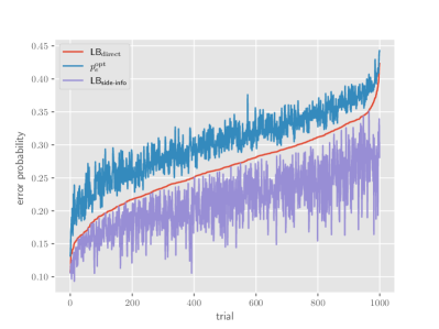
Figure 1: Numerical comparison of lower bounds with $d=2$, $X$ taking 10 values, and $\pi=1/2$.

For each trial, $d=2$ and $\alpha_{1}$ is drawn from $[0,1]$ uniformly at random, and $\alpha_{2}=1-\alpha_{1}$ (equivalently, $(\alpha_{1},\alpha_{2})$ follow the 2-dimensional symmetric Dirichlet distribution). The distributions $f_{1}$, $f_{2}$, $g_{1}$, $g_{2}$ follow the $10$-dimensional symmetric Dirichlet distribution independently. All these distributions are generated independently for each trial. The trials are sorted in the increasing order of $\mathsf{LB}_{\text{direct}}$. It is shown that $\mathsf{LB}_{\text{direct}}$ is usually better than $\mathsf{LB}_{\text{side-info}}$ for random mixtures. Note the following example shows this is not always the case. Equivalently, it shows that $\mathsf{LB}_{\text{direct}}$ is not a concave function of $(f,g)$.

Example 2

Consider discrete distributions with probability mass functions $f=(\frac{1}{3},\frac{1}{3},\frac{1}{3})$ and $g=(\frac{1}{2},\frac{1}{3},\frac{1}{6})$. Note the two distributions can be decomposed into mixtures as

$$f=\frac{2}{3}\left(\frac{1}{2},0,\frac{1}{2}\right)+\frac{1}{3}(0,1,0),$$

$$g=\frac{2}{3}\left(\frac{3}{4},0,\frac{1}{4}\right)+\frac{1}{3}(0,1,0).$$

Then for $\pi=1/2$, we have $\mathsf{LB}_{\text{direct}}\approx 0.4246$ and $\mathsf{LB}_{\text{side-info}}\approx 0.4385$. So $\mathsf{LB}_{\text{direct}}<\mathsf{LB}_{\text{side-info}}$.

V Application to dynamic ER networks

This section presents the random network prior used in [2]. As we will see, the direct lower bounds on the average error probability for such a prior require high-dimensional integration and are hard to compute even numerically, while the calculation of the lower bounds based on side information only involves the means and the determinants of the covariance matrices of the Gaussian mixture components.

Definition 1

A dynamic ER prior distribution, denoted by $\pi^{0}_{\mathsf{ER}}$, is the distribution of a signed ER graph scaled to a desired spectral radius if possible. Here the signed ER graph is a random graph whose edge weights take values in $\{-1,0,1\}$, with the locations of the edges determined by an ER graph and the signs equally likely. Formally, for given $n\in\mathbb{N}$, $p\in[0,1]$, and $r_{0}\in(0,1)$, let $R^{0}\in\{-1,1\}^{n\times n}$ be independent Rademacher random variables indicating the potential signs of the edges, and let $\chi^{0}\in\{0,1\}^{n\times n}$ be independent Bernoulli random variables with mean $p$ indicating the support. Then $\pi^{0}_{\mathsf{ER}}$ is defined to be the distribution of $s(R^{0}\circ\chi^{0})$, where $\circ$ denotes the Hadamard (entrywise) product and $s\colon\{-1,0,1\}^{n\times n}\to\mathbb{R}^{n\times n}$ defined by (recall $r(\cdot)$ is the spectral radius)

$$s(A)\triangleq\begin{cases}r_{0}\frac{A}{r(A)}&\text{if }r(A)\neq 0,\\ A&\text{if }r(A)=0.\end{cases}$$

Note $R^{0}\circ\chi^{0}$ can have a spectral radius of zero, in which case scaling cannot achieve the desired spectral radius $r_{0}$. Also note $\pi^{0}_{\mathsf{ER}}$ is symmetric in the sense of Remark 3.

To apply the direct lower bound in Proposition 2 one needs to calculate the $\rho_{ij}$’s, which are based on high-dimensional Gaussian components mixed with mixture weights from the dynamic ER networks. As a result, even numerical estimation is highly non-trivial.

Alternatively, to use Proposition 3 we need to find suitable side information for the BHT $\chi^{0}_{ij}=0$ vs. $\chi^{0}_{ij}=1$. Borrowing terminology from game theory, let $\chi^{0}_{-ij}$ be all the entries except the $(i,j)$th in $\chi^{0}$, defined by

$$\chi^{0}_{-ij}=(\chi^{0}_{i^{\prime}j^{\prime}}:i^{\prime},j^{\prime}\in[n],~{}(i^{\prime},j^{\prime})\neq(i,j)).$$

Because $R^{0}$ and $\chi^{0}_{-ij}$ are independent of $\chi^{0}_{ij}$, a natural choice of the side information is $(R^{0},\chi^{0}_{-ij})$. With a slight abuse of notation we write $\pi^{0}_{\mathsf{ER}}(R,\chi_{-ij})\triangleq\operatorname{\mathbb{P}}\{R^{0}=R,\chi^{0}_{-ij}=\chi_{-ij}\}$. Propositions 1 and 3 then yield the following bound on the average network-level error probability for the dynamics ER networks.

Proposition 4

Under $\pi^{0}_{\mathsf{ER}}$ for any estimator $\widehat{\chi}$ and any $\pi$,

$$\quad\pi\epsilon^{-}+(1-\pi)\epsilon^{+}$$

$$\geq\frac{1}{2}\left(1-\frac{1}{n^{2}}\sum_{i,j}\sum_{R,\chi_{-ij}}\pi^{0}_{\mathsf{ER}}(R,\chi_{-ij})\sqrt{1-4\pi(1-\pi)\rho_{i,j,R,\chi_{-ij}}^{2}}\right),$$

where $\rho_{i,j,R,\chi_{-ij}}$ is the BC for the following two mean zero Gaussian distributions: The conditional distribution of $Y$ given $R^{0}=R,\chi^{0}_{-ij}=\chi_{-ij},\chi^{0}_{ij}=0$ vs. the conditional distribution of $Y$ given $R^{0}=R,\chi^{0}_{-ij}=\chi_{-ij},\chi^{0}_{ij}=1$.

The bound in Proposition 4 involves an expectation over the probability distribution of the dynamic ER network, and can be readily estimated by Monte Carlo simulation.

VI Numerical results

VI-A Algorithms

Let

$$\Phi(0)=\begin{pmatrix}Y(0)\\ Y(1)\\ \vdots\\ Y(T-1)\end{pmatrix},\quad\Phi(1)=\begin{pmatrix}Y(1)\\ Y(2)\\ \vdots\\ Y(T)\end{pmatrix}.$$

VI-A1 lasso

The lasso algorithm solves the optimization problem

$$\operatorname*{minimize}_{A_{j}}\frac{1}{2T}\|\Phi_{j}(1)-\Phi(0)A_{j}\|_{2}^{2}+\lambda\|A_{j}\|_{1},$$

where $A_{j}$ and $\Phi_{j}(1)$ are the $j$th columns of $A$ and $\Phi(1)$, respectively, and $\lambda\geq 0$ is the regularization parameter. If $\Phi(0)^{*}\Phi(0)$ is invertible, the minimizer $\hat{A}_{j}^{\mathsf{lasso}}$ is unique. Write $\hat{A}_{j}^{\mathsf{lasso}}=\left(\hat{A}_{ij}^{\mathsf{lasso}}\colon i\in[n]\right)$. Then the estimated support matrix is $\widehat{\chi}^{\mathsf{lasso}}$ defined by $\widehat{\chi}_{ij}^{\mathsf{lasso}}=\mathbb{I}(\{\hat{A}_{ij}^{\mathsf{lasso}}\neq 0\})$. We implement lasso using scikit-learn [18].

VI-A2 oCSE

oCSE was proposed in [2]. For each target vertex $j$, its parent set is discovered greedily one at a time by finding the vertex whose column in $\Phi(0)$ together with the other chosen columns fits $\Phi_{j}(1)$ the best in the least squares sense. This discovery stage terminates when the improvement in the residual fails a permutation test with some threshold $\theta.$

VI-B Dynamic ER graphs

Comparisons of the receiver operating characteristic (ROC) curves of lasso and oCSE by varying the parameters $\lambda$ and $\theta$ and the upper bounds on the ROC curve resulted from Proposition 4 on dynamic ER graphs are shown in Figs. 2 and 3.

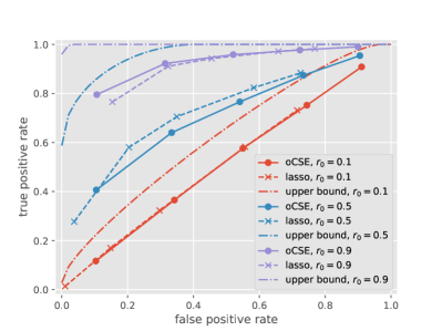
Figure 2: ROC curves of oCSE and lasso and the upper bound based on $\mathsf{LB}_{\text{side-info}}$ for dynamic ER graphs with $n=10$, $p=0.2$, $T=20$, and $\nu^{2}=0$, averaged over 100 simulations.

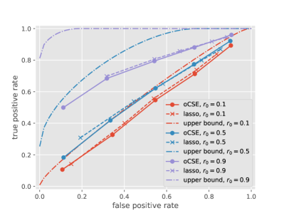
Figure 3: ROC curves of oCSE and lasso and the upper bound based on $\mathsf{LB}_{\text{side-info}}$ for dynamic ER graphs with $n=10$, $p=0.2$, $T=20$, and $\nu^{2}=1$, averaged over 100 simulations.

The simulation code can be found at [19].

VII Discussion

There is a significant gap between the information lower bound (upper bound on the ROC curve) and the algorithm performance, especially for small spectral radius (high signal-to-noise ratio) settings. Further research to close the gap is warranted.

Appendix A Mutual incoherence property in dynamic ER networks

For a covariance matrix $Q$, let $\mathcal{A}_{j}$ be the nonzero index set of column $j$ of $Q$. The mutual incoherence property in [4] requires that $\mathsf{MIP}\leq 1-\gamma_{0}$ for some positive $\gamma_{0}$, where

$$\mathsf{MIP}\triangleq\max_{1\leq j\leq n}\max_{i\notin\mathcal{A}_{j}}\|Q_{i,\mathcal{A}_{j}}Q_{\mathcal{A}_{j},\mathcal{A}_{j}}^{-1}\|_{1}.$$

For the dynamic ER networks as defined in Definition 1 starting from an all-zero state, the average MIP at time $T$ is shown in Fig. 4. It can be seen that the average MIP can be greater than $1$. As a result, the mutual incoherence property does not hold in general.

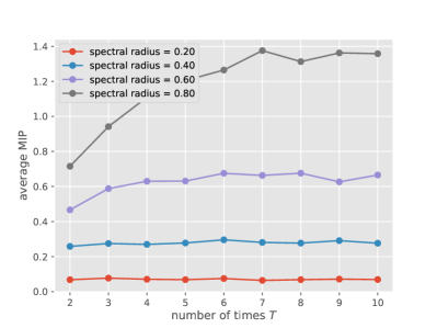
Figure 4: Average mutual incoherence parameters for dynamic ER networks with 200 vertices and 0.05 probability of connection. Each point is averaged over 10 simulations.

Appendix B Bhattacharyya bounds on average error probability for BHT

This section provides a proof of Lemma 1 and discusses the (non)-concavity properties of the related quantities in BHT.

Proof:

Let $\bar{\pi}\triangleq 1-\pi$. Integrating the identity $\pi f(y)+\bar{\pi}g(y)=2((\pi f(y))\wedge(\bar{\pi}g(y)))+|\pi f(y)-\bar{\pi}g(y)|$ over $y$ yields

$$1=2p_{e}^{\mathrm{opt}}+\int|\pi f(y)-\bar{\pi}g(y)|\mathop{}\!\mathrm{d}y.$$ (9)

The Cauchy–Schwarz inequality yields

$$\quad\int|\pi f(y)-\bar{\pi}g(y)|\mathop{}\!\mathrm{d}y$$

$$=\int\left|\sqrt{\pi f(y)}+\sqrt{\bar{\pi}g(y)}\right|\cdot\left|\sqrt{\pi f(y)}-\sqrt{\bar{\pi}g(y)}\right|\mathop{}\!\mathrm{d}y$$

$$\leq\sqrt{\int\left(\sqrt{\pi f(y)}+\sqrt{\bar{\pi}g(y)}\right)^{2}\mathop{}\!\mathrm{d}y}$$

$$\quad\cdot\sqrt{\int\left(\sqrt{\pi f(y)}-\sqrt{\bar{\pi}g(y)}\right)^{2}\mathop{}\!\mathrm{d}y}$$

$$=\sqrt{(1+2\sqrt{\pi\bar{\pi}}\rho)(1-2\sqrt{\pi\bar{\pi}}\rho)}$$

$$=\sqrt{1-4\pi\bar{\pi}\rho^{2}}.$$ (10)

Combining (9) and (10) yields

$$p_{e}^{\mathrm{opt}}\geq\frac{1}{2}\left[1-\sqrt{1-4\pi\bar{\pi}\rho^{2}}\right].$$

For the other direction, note that $(\pi f(y))\wedge(\bar{\pi}g(y))\leq\sqrt{\pi\bar{\pi}f(y)g(y)}$. Integrating over $y$ yields $p_{e}^{\mathrm{opt}}\leq\sqrt{\pi\bar{\pi}}\rho$.

Using the fact $\sqrt{1-u}\leq 1-\frac{u}{2}$ for $0\leq u\leq 1$ (square both sides to check), one gets $\frac{1}{2}(1-\sqrt{1-4\pi(1-\pi)\rho^{2}})\geq\pi(1-\pi)\rho^{2}$ (see also eq. (III.C.23) in Section III.C.2 of [20]).

Proof of the tensorization of BC is left to the reader. ∎

In the rest of this section we study the joint concavity of the average error probability and its upper and lower bounds in Lemma 1 in terms of the distributions $f$ and $g$. The following two lemmas show that the minimum average error probability and the upper bound are jointly concave in the two distributions. The two lower bounds are not concave in general per Example 2, but Proposition 5 shows $\rho^{2}$ is jointly concave in a binary case. Besides, Proposition 6 shows $\rho^{2}$ is concave in one distribution with the other fixed.

Lemma 2

For fixed $\pi$, the minimum average error probability $p_{e}^{\mathrm{opt}}$ in (5) is jointly concave in $f$ and $g$.

Proof:

For any $f_{1}$, $f_{2}$, $g_{1}$, $g_{2}$, and $\alpha$, let $f^{\prime}=\alpha f_{1}+(1-\alpha)f_{2}$ and let $g^{\prime}=\alpha g_{1}+(1-\alpha)g_{2}$. Then $f^{\prime}$ and $g^{\prime}$ are the mixture distributions of $f_{1}$, $f_{2}$ and $g_{1}$, $g_{2}$ with mixture weights $\alpha$ and $1-\alpha$. It then suffices to show for any $f_{1}$, $f_{2}$, $g_{1}$, $g_{2}$, and $\alpha$, we have

$$p_{e}^{\mathrm{opt}}(f^{\prime},g^{\prime})\geq\alpha p_{e}^{\mathrm{opt}}(f_{1},g_{1})+(1-\alpha)p_{e}^{\mathrm{opt}}(f_{2},g_{2}).$$ (11)

Indeed, the left-hand side of (11) is the optimal average error probability based on an observation of the two mixture distributions, while the right-hand side of (11) is the optimal average error probability based on the observation as well as the side information of a binary random variable indicating the mixture component. Since side information cannot hurt, we obtain (11). ∎

Lemma 3

The BC $\rho$ is jointly concave in $f$ and $g$.

Proof:

It is easy to see that the mapping $\phi\colon(x,y)\mapsto\sqrt{xy}$ is jointly concave by checking the Hessian. Then $\rho$ is also jointly concave because a summation or integration of concave functions is still concave. ∎

Example 2 shows $\mathsf{LB}_{\text{direct}}$ defined in (7) is not concave. The same example also demonstrates that $\rho^{2}$ is not concave. The following proposition shows that $\rho^{2}$ is however indeed concave for discrete distributions taking only two values.

Proposition 5

For binary-valued distributions $f$ and $g$, the BC $\rho^{2}(f,g)=\sqrt{f_{1}g_{1}}+\sqrt{f_{2}g_{2}}$ is jointly concave in $(f,g)$.

The proof can be done by checking the Hessian is negative semi-definite and is left to the reader.

Proposition 6

$\rho^{2}(f,\cdot)$ is concave for fixed $f$.

Proof:

Applying the reverse Minkowski inequality immediately yields the result. ∎

Appendix C Bounds on the area under the ROC curve

This paper presents lower bounds on error probabilities which were shown as upper bounds on the ROC curve. This section briefly describes the corresponding upper bounds on the area under the ROC curve. For the Bayes optimal decision rules $\delta(\pi)$ defined in Section III-A, the area under the ROC curve, denoted by AUC, is traced out by varying $\pi$ for the pair $(1-P^{-}_{\delta(\pi)},P^{+}_{\delta(\pi)})$. Lemma 1 implies the following upper bound on AUC.

Corollary 1

$\mathsf{AUC}\leq 1-\rho^{4}/6$.

Proof:

For any $\pi\in[0,1]$ and any $\alpha\in[0,1]$, let $\bar{\pi}=1-\pi$ and $\bar{\alpha}=1-\alpha$. By Lemma 1,

$$\alpha P^{-}_{\delta(\pi)}+\bar{\alpha}P^{+}_{\delta(\pi)}\geq\alpha\bar{\alpha}\rho^{2}.$$

Using the fact that for any nonnegative $a$, $b$, and $c$,

$$(\forall\alpha\in[0,1],\alpha a+\bar{\alpha}b\geq\alpha\bar{\alpha}c)\iff\sqrt{a}+\sqrt{b}\geq\sqrt{c},$$

we can eliminate the parameter $\alpha$ to get $P^{-}_{\delta(\pi)}\geq\left(\rho-\sqrt{P^{+}_{\delta(\pi)}}\right)^{2}$. Then by excluding the impossible region we have $\mathsf{AUC}\leq 1-\int_{0}^{\rho^{2}}(\rho-\sqrt{x})^{2}\mathop{}\!\mathrm{d}x=1-\rho^{4}/6$. ∎

Similarly, the tighter lower bound on $p_{e}^{\mathrm{opt}}$ in Lemma 1(a) implies a tighter upper bound on AUC. The tighter AUC bound does not have a nice analytical form, but can nevertheless be numerically computed. The two bounds and the bound from Shapiro [21] ($\mathsf{AUC}\leq 1-(1-\sqrt{1-\rho^{2}})^{2}/2$) are shown in Fig. 5.

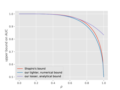
Figure 5: Comparison of upper bounds on AUC.

It can be seen that our numerical bound outperforms Shapiro’s bound for all value of $\rho$, and our simple analytical bound in Corollary 1 also slightly outperforms Shapiro’s bound when $\rho<0.65$.

References

- [1] D. Marbach, J. C. Costello, R. Küffner, N. M. Vega, R. J. Prill, D. M. Camacho, K. R. Allison, M. Kellis, J. J. Collins, and G. Stolovitzky, “Wisdom of crowds for robust gene network inference,” Nat Methods, vol. 9, no. 8, pp. 796–804, Jul. 2012.
- [2] J. Sun, D. Taylor, and E. M. Bollt, “Causal network inference by optimal causation entropy,” SIAM Journal on Applied Dynamical Systems, vol. 14, no. 1, pp. 73–106, Jan. 2015.
- [3] M. Simchowitz, H. Mania, S. Tu, M. I. Jordan, and B. Recht, “Learning without mixing: Towards a sharp analysis of linear system identification,” CoRR, vol. abs/1802.08334, 2018. [Online]. Available: http://arxiv.org/abs/1802.08334
- [4] S. Fattahi and S. Sojoudi, “Sample complexity of sparse system identification problem,” CoRR, vol. abs/1803.07753, 2018. [Online]. Available: http://arxiv.org/abs/1803.07753
- [5] S. Fattahi, N. Matni, and S. Sojoudi, “Learning sparse dynamical systems from a single sample trajectory,” CoRR, vol. abs/1904.09396, 2019. [Online]. Available: http://arxiv.org/abs/1904.09396
- [6] S. Oymak and N. Ozay, “Non-asymptotic identification of LTI systems from a single trajectory,” in 2019 American Control Conference (ACC). IEEE, Jul. 2019.
- [7] S. Lale, K. Azizzadenesheli, B. Hassibi, and A. Anandkumar, “Logarithmic regret bound in partially observable linear dynamical systems,” CoRR, vol. abs/2003.11227, 2020. [Online]. Available: https://arxiv.org/abs/2003.11227
- [8] J. Bento, M. Ibrahimi, and A. Montanari, “Learning networks of stochastic differential equations,” in Advances in Neural Information Processing Systems (NIPS), 2010, pp. 172–180. [Online]. Available: http://papers.nips.cc/paper/4055-learning-networks-of-stochastic-differential-equations.pdf
- [9] J. Fuchs, “Recovery of exact sparse representations in the presence of bounded noise,” IEEE Transactions on Information Theory, vol. 51, no. 10, pp. 3601–3608, Oct. 2005.
- [10] J. Tropp, “Just relax: convex programming methods for identifying sparse signals in noise,” IEEE Transactions on Information Theory, vol. 52, no. 3, pp. 1030–1051, Mar. 2006.
- [11] P. Zhao and B. Yu, “On model selection consistency of Lasso,” J Mach Learn Res, vol. 7, pp. 2541–2563, Nov. 2006.
- [12] N. Meinshausen and P. Bühlmann, “High-dimensional graphs and variable selection with the lasso,” The Annals of Statistics, vol. 34, no. 3, pp. 1436–1462, Jun. 2006.
- [13] M. J. Wainwright, “Sharp thresholds for high-dimensional and noisy sparsity recovery using -constrained quadratic programming (Lasso),” IEEE Transactions on Information Theory, vol. 55, no. 5, pp. 2183–2202, May 2009.
- [14] Y. Jedra and A. Proutiere, “Sample complexity lower bounds for linear system identification,” in 2019 IEEE 58th Conference on Decision and Control (CDC). IEEE, Dec. 2019.
- [15] J. Bento, M. Ibrahimi, and A. Montanari, “Information theoretic limits on learning stochastic differential equations,” in 2011 IEEE International Symposium on Information Theory Proceedings. IEEE, Jul. 2011.
- [16] J. B. A. Periera and M. Ibrahimi, “Support recovery for the drift coefficient of high-dimensional diffusions,” IEEE Transactions on Information Theory, vol. 60, no. 7, pp. 4026–4049, Jul. 2014.
- [17] T. Kailath, “The divergence and Bhattacharyya distance measures in signal selection,” IEEE Transactions on Communications, vol. 15, no. 1, pp. 52–60, Feb. 1967.
- [18] F. Pedregosa, G. Varoquaux, A. Gramfort, V. Michel, B. Thirion, O. Grisel, M. Blondel, P. Prettenhofer, R. Weiss, V. Dubourg, J. Vanderplas, A. Passos, D. Cournapeau, M. Brucher, M. Perrot, and E. Duchesnay, “Scikit-learn: Machine learning in Python,” Journal of Machine Learning Research, vol. 12, pp. 2825–2830, 2011.
- [19] X. Kang, “Causal network inference simulations,” Feb. 2021. [Online]. Available: https://github.com/Veggente/net-inf-eval
- [20] H. V. Poor, An Introduction to Signal Detection and Estimation. Springer-Verlag New York, 1994.
- [21] J. H. Shapiro, “Bounds on the area under the ROC curve,” Journal of the Optical Society of America A, vol. 16, no. 1, p. 53, Jan. 1999.