Measurements of Partial Branching Fractions of Inclusive $B\to X_{u}\,\ell^{+}\,\nu_{\ell}$ Decays with Hadronic Tagging

Abstract

We present measurements of partial branching fractions of inclusive semileptonic $B\to X_{u}\,\ell^{+}\,\nu_{\ell}$ decays using the full Belle data set of 711 fb^-1 of integrated luminosity at the $\Upsilon(4S)$ resonance and for $\ell=e,\mu$. Inclusive semileptonic $B\to X_{u}\,\ell^{+}\,\nu_{\ell}$ decays are CKM suppressed and measurements are complicated by the large background from CKM-favored $B\to X_{c}\,\ell^{+}\,\nu_{\ell}$ transitions, which have a similar signature. Using machine learning techniques, we reduce this and other backgrounds effectively, whilst retaining access to a large fraction of the $B\to X_{u}\,\ell^{+}\,\nu_{\ell}$ phase space and high signal efficiency. We measure partial branching fractions in three phase-space regions covering about 31% to 86% of the accessible $B\to X_{u}\,\ell^{+}\,\nu_{\ell}$ phase space. The most inclusive measurement corresponds to the phase space with lepton energies of $E_{\ell}^{B}>1$ GeV, and we obtain $\Delta\mathcal{B}(B\to X_{u}\ell^{+}\,\nu_{\ell})=\left(1.59\pm 0.07\pm 0.16\right)\times 10^{-3}$ from a two-dimensional fit of the hadronic mass spectrum and the four-momentum-transfer squared distribution, with the uncertainties denoting the statistical and systematic error. We find $\left|V_{ub}\right|=\left(4.10\pm 0.09\pm 0.22\pm 0.15\right)\times 10^{-3}$ from an average of four calculations for the partial decay rate with the third uncertainty denoting the average theory error. This value is higher but compatible with the determination from exclusive semileptonic decays within 1.3 standard deviations. In addition, we report charmless inclusive partial branching fractions separately for $B^{+}$ and $B^{0}$ mesons as well as for electron and muon final states. No isospin breaking or lepton flavor universality violating effects are observed.

I introduction

Precision measurements of the absolute value of the Cabibbo-Kobayashi-Maskawa (CKM) matrix element $V_{ub}$ are important to challenge the Standard Model of particle physics (SM) Cabibbo (1963); Kobayashi and Maskawa (1973). In the SM, the CKM matrix is a $3\times 3$ unitary matrix and responsible for the known charge-parity (CP) violating effects in the quark sector Zyla et al. (2020a). There are indications of CP violation in the neutrino sector Abe et al. (2020), but it remains unclear if both sources of CP violation are sufficient to explain the matter dominance of today’s universe. This motivates the search for new sources of CP-violating phenomena. If such exist in the form of heavy exotic particles that couple to quarks in some form, their presence might alter the properties of measurements constraining the unitarity of the CKM matrix Kou et al. (2019). Precise measurements of $|V_{ub}|$ and the CKM angle $\gamma=\phi_{3}$ are imperative to isolate such effects, as their measurements involve tree-level processes, which are expected to remain unaffected by new physics and thus provide an unbiased measure for the amount of CPV due to the Kobayashi-Maskawa (KM) mechanism Kobayashi and Maskawa (1973) alone.

Charmless semileptonic decays of $\mathit{{B}{}_{\mspace{-3.0mu}\scriptstyle{}}^{\mspace{-1.0mu}\scriptstyle{}}}$ mesons provide a clean avenue to measure $|V_{ub}|$, as their decay rate is theoretically better understood than purely hadronic transitions and their decay signature is more accessible than leptonic $\mathit{{B}{}_{\mspace{-3.0mu}\scriptstyle{}}^{\mspace{-1.0mu}\scriptstyle{}}}$ meson decays. The existing measurements either focus on exclusive final states, with $B\to\pi\,\ell^{+}\,\nu_{\ell}$ Amhis et al. (2019) and the ratio of $\Lambda_{b}\to p\,\mu^{+}\,\nu_{\mu}$ and $\Lambda_{b}\to\Lambda_{c}\,\mu^{+}\,\nu_{\mu}$ Aaij et al. (2015) providing the most precise measurements to date, and measurements reconstructing the $B\to X_{u}\,\ell^{+}\,\nu_{\ell}$ decay fully inclusively. Central for both approaches are reliable predictions of the (partial) decay rates $\Delta\Gamma(B\to X_{u}\,\ell^{+}\,\nu_{\ell})$ (omitting the CKM factor) from theory to convert measured (partial or full) branching fractions, $\Delta\mathcal{B}(B\to X_{u}\,\ell^{+}\,\nu_{\ell})$, into measurements of $|V_{ub}|$ via

$$|V_{ub}|=\sqrt{\frac{\Delta\mathcal{B}(B\to X_{u}\,\ell^{+}\,\nu_{\ell})}{\tau_{B}\,\Delta\Gamma(B\to X_{u}\,\ell^{+}\,\nu_{\ell})}}\,,$$

with $\tau_{B}$ denoting the $B$ meson lifetime. For exclusive measurements, the non-perturbative parts of the decay rates can be reliably predicted by lattice QCD Aoki et al. (2020) or light-cone sum rules Bharucha (2012) and constrained by the measurements of the decay dynamics. The determination of $|V_{ub}|$ using inclusive decays is very challenging due to the large background from the CKM-favored $B\to X_{c}\,\ell^{+}\,\nu_{\ell}$ process. Both processes have a very similar decay signature in the form of a high momentum lepton, a hadronic system, and missing energy from the neutrino that escapes detection. Figure 1 shows an illustration of both processes for a $B^{0}$-meson decay. A clear separation of the processes is only possible in kinematic regions where $B\to X_{c}\,\ell^{+}\,\nu_{\ell}$ is kinematically forbidden. In these regions, however, non-perturbative shape functions enter the description of the decay dynamics, making predictions for the decay rates dependent on the precise modeling. These functions parametrize at leading order the Fermi motion of the $b$ quark inside the $B$ meson. Properties of the leading-order $\Lambda_{\mathrm{QCD}}/m_{b}$ shape function can be determined using the photon energy spectrum of $B\to X_{s}\,\gamma$ decays and moments of the lepton energy or hadronic invariant mass in semileptonic $B$ decays Gambino and Uraltsev (2004); Bauer et al. (2004); Benson et al. (2005), but the modeling of both the leading and subleading shape functions introduces large theory uncertainties on the decay rate. In the future, more model-independent approaches aim to directly measure the leading-order shape function Bernlochner et al. (2020); Gambino et al. (2016).

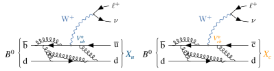
Figure 1: The CKM suppressed and favored inclusive semileptonic processes $B\to X_{u}\,\ell^{+}\,\nu_{\ell}$ (left) and $B\to X_{c}\,\ell^{+}\,\nu_{\ell}$ (right) for a $B^{0}$ meson decay.

As such methods are not yet realized, it is beneficial to extend the measurement region as much as possible into the $B\to X_{c}\,\ell^{+}\,\nu_{\ell}$ dominated phase space. This was done, e.g., by Refs. Lees et al. (2012); Urquijo et al. (2010). This reduces the theory uncertainties on the predicted partial rates Lange et al. (2005a); Gambino et al. (2007); Andersen and Gardi (2006); Gardi (2008); Aglietti et al. (2009, 2007), although making the measurement more prone to systematic uncertainties. This strategy is also adopted in the measurement described in this paper.

The corresponding world averages of $|V_{ub}|$ from both exclusive and inclusive determinations are Amhis et al. (2019):

$$|V_{ub}^{\mathrm{excl.}}| =\left(3.67\pm 0.09\pm 0.12\right)\times 10^{-3}\,,$$ (1)

$$|V_{ub}^{\mathrm{incl.}}| =\left(4.32\pm 0.12{}^{+0.12}_{-0.13}\right)\times 10^{-3}\,.$$ (2)

Here the uncertainties are experimental and from theory. Both world averages exhibit a disagreement of about 3 standard deviations between them. This disagreement is limiting the reach of present-day precision tests of the KM mechanism and searches for loop-level new physics, see e.g. Ref. Bona et al. (2020) for a recent analysis. For a more complete review the interested reader is referred to Refs. Dingfelder and Mannel (2016); Zyla et al. (2020b).

One important experimental method to extend the probed $B\to X_{u}\,\ell^{+}\,\nu_{\ell}$ phase space into regions dominated by $B\to X_{c}\,\ell^{+}\,\nu_{\ell}$ transitions is the full reconstruction of the second $\mathit{{B}{}_{\mspace{-3.0mu}\scriptstyle{}}^{\mspace{-1.0mu}\scriptstyle{}}}$ meson of the $e^{+}\,e^{-}\to\Upsilon(4S)\to B\bar{B}$ process. This process is referred to as “tagging” and allows for the reconstruction of the hadronic $X$ system of the semileptonic process. In addition, the neutrino four-momentum can be reconstructed. Properties of both are instrumental to distinguish $B\to X_{u}\,\ell^{+}\,\nu_{\ell}$ and $B\to X_{c}\,\ell^{+}\,\nu_{\ell}$ processes. In this manuscript the reconstruction of the second $\mathit{{B}{}_{\mspace{-3.0mu}\scriptstyle{}}^{\mspace{-1.0mu}\scriptstyle{}}}$ meson and the separation of $B\to X_{u}\,\ell^{+}\,\nu_{\ell}$ from $B\to X_{c}\,\ell^{+}\,\nu_{\ell}$ processes were carried out using machine learning approaches. Several neural networks were trained to identify correctly reconstructed tag-side $\mathit{{B}{}_{\mspace{-3.0mu}\scriptstyle{}}^{\mspace{-1.0mu}\scriptstyle{}}}$ mesons. The distinguishing variables of the classification algorithm were carefully selected in order not to introduce a bias in the measured partial branching fractions. In addition, the modeling of backgrounds was validated in $B\to X_{c}\,\ell^{+}\,\nu_{\ell}$ enriched selections. We report the measurement of three partial branching fractions, covering 31% - 86% of the accessible $B\to X_{u}\,\ell^{+}\,\nu_{\ell}$ phase space. The measurement of fully differential distributions, which allow one to determine the leading and subleading shape functions, is left for future work.

The main improvement over the previous Belle result of Ref. Urquijo et al. (2010) lies in the adoption of a more efficient tagging algorithm for the reconstruction of the second $B$ meson and the improvements of the $B\to X_{u}\,\ell^{+}\,\nu_{\ell}$ signal and $B\to X_{c}\,\ell^{+}\,\nu_{\ell}$ background descriptions. In addition, the full Belle data set of 711 fb^-1 is analyzed and we avoid the direct use of kinematic properties of the candidate semileptonic decay in the background suppression. After the final selection we retain a factor of approximatively 1.8 times more signal events than the previous analysis with a ca. 20% improved purity.

The remainder of this manuscript is organized as follows: Section II provides an overview of the data set and the simulated signal and background samples, that were used in the analysis. Section III details the analysis strategy and reconstruction of the hadronic $X$ system of the semileptonic decay. Section IV introduces the fit procedure used to separate $B\to X_{u}\,\ell^{+}\,\nu_{\ell}$ signal from background contributions. Section V lists the systematic uncertainties affecting the measurements and Section VI summarizes sideband studies central to validate the modeling of the crucial $B\to X_{c}\,\ell^{+}\,\nu_{\ell}$ background processes. Finally, Section VII shows the selected signal events and compares them with the expectation from simulation. In Section VIII the measured partial branching fractions and subsequent values of $|V_{ub}|$ are discussed. Section IX presents our conclusions.

II Data Set and Simulated Samples

The analysis utilizes the full Belle data set of $(772\pm 10)\times 10^{6}$ $\mathit{{B}{}_{\mspace{-3.0mu}\scriptstyle{}}^{\mspace{-1.0mu}\scriptstyle{}}}$ meson pairs, which were produced at the KEKB accelerator complex Kurokawa and Kikutani (2003) with a center-of-mass energy of $\sqrt{s}=$10.58\text{\,}\mathrm{G}\mathrm{e}\mathrm{V}$$ corresponding to the $\Upsilon(4S)$ resonance. In addition, $79\text{\,}\mathrm{f}\mathrm{b}^{-1}$ of collision events recorded $60\text{\,}\mathrm{M}\mathrm{e}\mathrm{V}$ below the $\Upsilon(4S)$ resonance peak are used to derive corrections and for cross-checks.

The Belle detector is a large-solid-angle magnetic spectrometer that consists of a silicon vertex detector, a 50-layer central drift chamber (CDC), an array of aerogel threshold Cherenkov counters (ACC), a barrel-like arrangement of time-of-flight scintillation counters (TOF), and an electromagnetic calorimeter composed of CsI(Tl) crystals (ECL) located inside a superconducting solenoid coil that provides a $1.5\text{\,}\mathrm{T}$ magnetic field. An iron flux return located outside of the coil is instrumented to detect $K^{0}_{L}$ mesons and to identify muons (KLM). A more detailed description of the detector and its layout and performance can be found in Ref. (Abashian et al., 2002a) and in references therein.

Charged tracks are identified as electron or muon candidates by combining the information of multiple subdetectors into a lepton identification likelihood ratio, $\mathcal{L}_{\mathrm{LID}}$. For electrons, the most important identifying features are the ratio of the energy deposition in the ECL with respect to the reconstructed track momentum, the energy loss in the CDC, the shower shape in the ECL, the quality of the geometrical matching of the track to the shower position in the ECL, and the photon yield in the ACC (Hanagaki et al., 2002). Muon candidates can be identified from charged track trajectories extrapolated to the outer detector. The most important identifying features are the difference between expected and measured penetration depth as well as the transverse deviation of KLM hits from the extrapolated trajectory (Abashian et al., 2002b). Charged tracks are identified as pions or kaons using a likelihood ratio $\mathcal{L}_{\mathrm{K/\pi\,\mathrm{ID}}}=\mathcal{L}_{\mathrm{K\,\mathrm{ID}}}/\left(\mathcal{L}_{\mathrm{K\,\mathrm{ID}}}+\mathcal{L}_{\mathrm{\pi\,\mathrm{ID}}}\right)$. The most important identifying features of the kaon ($\mathcal{L}_{\mathrm{K\,\mathrm{ID}}}$) and pion ($\mathcal{L}_{\mathrm{\pi\,\mathrm{ID}}}$) likelihoods for low momentum particles with transverse momentum below 1 GeV in the laboratory frame are the recorded energy loss by ionization, $\mathrm{d}E/\mathrm{d}x$, in the CDC, and the time of flight information from the TOF. Higher-momentum kaon and pion classification relies on the Cherenkov light recorded in the ACC. In order to avoid the difficulties in understanding the efficiencies of reconstructing $K^{0}_{L}$ mesons, they are not explicitly reconstructed or used in this analysis.

Photons are identified as energy depositions in the ECL, vetoing clusters to which an associated track can be assigned. Only photons with an energy deposition of $E_{\gamma}$ $>$100\text{\,}\mathrm{M}\mathrm{e}\mathrm{V}$$, $150\text{\,}\mathrm{M}\mathrm{e}\mathrm{V}$, and $50\text{\,}\mathrm{M}\mathrm{e}\mathrm{V}$ in the forward endcap, backward endcap and barrel part of the calorimeter, respectively, are considered. We reconstruct $\pi^{0}$ candidates from photon candidates. The invariant mass is required to fall inside a window of $m_{\gamma\gamma}\in[0.12,0.15]\,\text{GeV}$, which corresponds to about 2.5 times the $\pi^{0}$ mass resolution.

Monte Carlo (MC) samples of $\mathit{{B}{}_{\mspace{-3.0mu}\scriptstyle{}}^{\mspace{-1.0mu}\scriptstyle{}}}$ meson decays and continuum processes ($e^{+}e^{-}\to q\bar{q}$ with $q=u,d,s,c$) are simulated using the EvtGen generator (Lange, 2001). These samples are used to evaluate reconstruction efficiencies and acceptance, and to estimate background contaminations. The sample sizes used correspond to approximately ten and five times, respectively, the Belle collision data for $\mathit{{B}{}_{\mspace{-3.0mu}\scriptstyle{}}^{\mspace{-1.0mu}\scriptstyle{}}}$ meson and continuum decays. The interactions of particles traversing the detector are simulated using Geant3 (Brun et al., 1987). Electromagnetic final-state radiation is simulated using the PHOTOS (Barberio et al., 1991) package for all charged final-state particles. The efficiencies in the MC are corrected using data-driven methods to account for, e.g., differences in identification and reconstruction efficiencies.

Table 1: Branching fractions for $B\to X_{u}\,\ell^{+}\,\nu_{\ell}$ and $B\to X_{c}\,\ell^{+}\,\nu_{\ell}$ background processes that were used are listed. More details on the applied corrections can be found in the text. We neglect the small contribution from $B^{+}\to D_{s}^{(*)}\,K^{+}\,\ell^{+}\,\nu_{\ell}$ which has a branching fraction of similar size as $B\to D\pi\pi\,\ell^{+}\,\nu_{\ell}$.

$\mathcal{B}$	Value $B^{+}$	Value $B^{0}$
$B\to X_{u}\,\ell^{+}\,\nu_{\ell}$
$B\to\pi\,\ell^{+}\,\nu_{\ell}$	$\left(7.8\pm 0.3\right)\times 10^{-5}$	$\left(1.5\pm 0.06\right)\times 10^{-4}$
$B\to\eta\,\ell^{+}\,\nu_{\ell}$	$\left(3.9\pm 0.5\right)\times 10^{-5}$	-
$B\to\eta^{\prime}\,\ell^{+}\,\nu_{\ell}$	$\left(2.3\pm 0.8\right)\times 10^{-5}$	-
$B\to\omega\,\ell^{+}\,\nu_{\ell}$	$\left(1.2\pm 0.1\right)\times 10^{-4}$	-
$B\to\rho\,\ell^{+}\,\nu_{\ell}$	$\left(1.6\pm 0.1\right)\times 10^{-4}$	$\left(2.9\pm 0.2\right)\times 10^{-4}$
$B\to X_{u}\,\ell^{+}\,\nu_{\ell}$	$\left(2.2\pm 0.3\right)\times 10^{-3}$	$\left(2.0\pm 0.3\right)\times 10^{-3}$
$B\to X_{c}\,\ell^{+}\,\nu_{\ell}$
$B\to D\,\ell^{+}\,\nu_{\ell}$	$\left(2.5\pm 0.1\right)\times 10^{-2}$	$\left(2.3\pm 0.1\right)\times 10^{-2}$
$B\to D^{*}\,\ell^{+}\,\nu_{\ell}$	$\left(5.4\pm 0.1\right)\times 10^{-2}$	$\left(5.1\pm 0.1\right)\times 10^{-2}$
$B\to D_{0}^{*}\,\ell^{+}\,\nu_{\ell}$	$\left(4.2\pm 0.8\right)\times 10^{-3}$	$\left(3.9\pm 0.7\right)\times 10^{-3}$
$(\hookrightarrow D\pi)$
$B\to D_{1}^{*}\,\ell^{+}\,\nu_{\ell}$	$\left(4.2\pm 0.8\right)\times 10^{-3}$	$\left(3.9\pm 0.8\right)\times 10^{-3}$
$(\hookrightarrow D^{*}\pi)$
$B\to D_{1}\,\ell^{+}\,\nu_{\ell}$	$\left(4.2\pm 0.3\right)\times 10^{-3}$	$\left(3.9\pm 0.3\right)\times 10^{-3}$
$(\hookrightarrow D^{*}\pi)$
$B\to D_{2}^{*}\,\ell^{+}\,\nu_{\ell}$	$\left(1.2\pm 0.1\right)\times 10^{-3}$	$\left(1.1\pm 0.1\right)\times 10^{-3}$
$(\hookrightarrow D^{*}\pi)$
$B\to D_{2}^{*}\,\ell^{+}\,\nu_{\ell}$	$\left(1.8\pm 0.2\right)\times 10^{-3}$	$\left(1.7\pm 0.2\right)\times 10^{-3}$
$(\hookrightarrow D\pi)$
$B\to D_{1}\,\ell^{+}\,\nu_{\ell}$	$\left(2.4\pm 1.0\right)\times 10^{-3}$	$\left(2.3\pm 0.9\right)\times 10^{-3}$
$(\hookrightarrow D\pi\pi)$
$B\to D\pi\pi\,\ell^{+}\,\nu_{\ell}$	$\left(0.6\pm 0.6\right)\times 10^{-3}$	$\left(0.6\pm 0.6\right)\times 10^{-3}$
$B\to D^{*}\pi\pi\,\ell^{+}\,\nu_{\ell}$	$\left(2.2\pm 1.0\right)\times 10^{-3}$	$\left(2.0\pm 1.0\right)\times 10^{-3}$
$B\to D\eta\,\ell^{+}\,\nu_{\ell}$	$\left(4.0\pm 4.0\right)\times 10^{-3}$	$\left(4.0\pm 4.0\right)\times 10^{-3}$
$B\to D^{*}\eta\,\ell^{+}\,\nu_{\ell}$	$\left(4.0\pm 4.0\right)\times 10^{-3}$	$\left(4.0\pm 4.0\right)\times 10^{-3}$
$B\to X_{c}\,\ell^{+}\,\nu_{\ell}$	$\left(10.8\pm 0.4\right)\times 10^{-2}$	$\left(10.1\pm 0.4\right)\times 10^{-2}$

The most important background processes are semileptonic $B\to X_{c}\,\ell^{+}\,\nu_{\ell}$ decays and continuum processes, which both can produce high-momentum leptons in a momentum range similar to the $B\to X_{u}\,\ell^{+}\,\nu_{\ell}$ process. The semileptonic background from $B\to X_{c}\,\ell^{+}\,\nu_{\ell}$ decays is dominated by $B\to D\,\ell^{+}\,\nu_{\ell}$ and $B\to D^{*}\,\ell^{+}\,\nu_{\ell}$ decays. The $B\to D\,\ell^{+}\,\nu_{\ell}$ decays are modeled using the BGL parametrization Boyd et al. (1995) with form factor central values and uncertainties taken from the fit in Ref. Glattauer et al. (2016). For $B\to D^{*}\,\ell^{+}\,\nu_{\ell}$   we use the BGL implementation proposed by Refs. Grinstein and Kobach (2017); Bigi et al. (2017) with form factor central values and uncertainties from the fit to the measurement of Ref. Waheed et al. (2019). Both backgrounds are normalized to the average branching fraction of Ref. Amhis et al. (2019) assuming isospin symmetry. Semileptonic $B\to D^{**}\,\ell^{+}\,\nu_{\ell}$ decays with $D^{**}=\{D_{0}^{*},D_{1}^{*},D_{1},D_{2}^{*}\}$ denoting the four orbitally excited charmed mesons are modeled using the heavy-quark-symmetry-based form factors proposed in Ref. Bernlochner and Ligeti (2017). We simulate all $D^{**}$ decays using masses and widths from Ref. Zyla et al. (2020c). For the branching fractions we adopt the values of Ref. Amhis et al. (2019) and correct them to account for missing isospin-conjugated and other established decay modes, following the prescription given in Ref. Bernlochner and Ligeti (2017). To correct for the fact that the measurements were carried out in the $D^{**\,0}\to D^{(*)+}\,\pi^{-}$ decay modes, we account for the missing isospin modes with a factor of

$$f_{\pi}=\frac{\mathcal{B}(\overline{D}^{**\,0}\to D^{(*)\,-}\pi^{+})}{\mathcal{B}(\overline{D}^{**\,0}\to\overline{D}^{(*)}\pi)}=\frac{2}{3}\,.$$ (3)

The measurements of the $B\to D_{2}^{*}\,\ell\bar{\nu}_{\ell}$ in Ref. Amhis et al. (2019) are converted to only account for the $\overline{D}_{2}^{*\,0}\to D^{*\,-}\pi^{+}$ decay. To also account for $\overline{D}_{2}^{*\,0}\to D^{-}\pi^{+}$ contributions, we apply a factor of Zyla et al. (2020c)

$$f_{D_{2}^{*}}=\frac{\mathcal{B}(\overline{D}_{2}^{*\,0}\to D^{-}\pi^{+})}{\mathcal{B}(\overline{D}_{2}^{*\,0}\to D^{*\,-}\pi^{+})}=1.54\pm 0.15\,.$$ (4)

The world average of $B\to D_{1}^{*}\,\ell\bar{\nu}_{\ell}$ given in Ref. Amhis et al. (2019) combines measurements, which show poor agreement, and the resulting probability of the combination is below 0.01%. Notably, the measurement of Ref. Liventsev et al. (2008) is in conflict with the measured branching fractions of Refs. Aubert et al. (2008); Abdallah et al. (2006) and with the expectation of $\mathcal{B}(B\to D_{1}^{*}\,\ell\bar{\nu}_{\ell})$ being of similar size than $\mathcal{B}(B\to D_{0}\,\ell\bar{\nu}_{\ell})$ Leibovich et al. (1998); Bigi et al. (2007). We perform our own average excluding Ref. Liventsev et al. (2008) and use

$$\mathcal{B}(B^{+}\to\overline{D}_{1}^{*\,0}(\to D^{*\,-}\pi^{+})\,\ell^{+}\nu_{\ell}) =\left(0.28\pm 0.06\right)\times 10^{-2}\,.$$ (5)

The world average of $B\to D_{1}\,\ell\bar{\nu}_{\ell}$ does not include contributions from prompt three-body decays of $D_{1}\to D\pi\pi$. We account for these using a factor Aaij et al. (2011)

$$f_{D_{1}}=\frac{\mathcal{B}(\overline{D}_{1}^{0}\to D^{*\,-}\pi^{+})}{\mathcal{B}(\overline{D}_{1}^{0}\to\overline{D}^{0}\pi^{+}\pi^{-})}=2.32\pm 0.54\,.$$ (6)

We subtract the contribution of $D_{1}\to D\pi\pi$ from the measured non-resonant plus resonant $B\to D\pi\pi\ell\bar{\nu}_{\ell}$ branching fraction of Ref. Lees et al. (2016). To account for missing isospin-conjugated modes of the three-hadron final states we adopt the prescription from Ref. Lees et al. (2016), which calculates an average isospin correction factor of

$$f_{\pi\pi} =\frac{\mathcal{B}(\overline{D}^{**\,0}\to\overline{D}^{(*)\,0}\pi^{+}\pi^{-})}{\mathcal{B}(\overline{D}^{**\,0}\to\overline{D}^{(*)}\pi\pi)}=\frac{1}{2}\pm\frac{1}{6}\,.$$ (7)

The uncertainty takes into account the full spread of final states ($f_{0}(500)\to\pi\pi$ or $\rho\to\pi\pi$ result in $f_{\pi\pi}=2/3$ and $1/3$, respectively) and the non-resonant three-body decays ($f_{\pi\pi}=3/7$). We further assume that

$$\mathcal{B}(\overline{D}_{2}^{*}\to\overline{D}\pi)+\mathcal{B}(\overline{D}_{2}^{*}\to\overline{D}^{*}\pi)=1\,,$$

$$\mathcal{B}(\overline{D}_{1}\to\overline{D}^{*}\pi)+\mathcal{B}(\overline{D}_{1}\to\overline{D}\pi\pi)=1\,,$$

$$\mathcal{B}(\overline{D}_{1}^{*}\to\overline{D}^{*}\pi)=1\,,\quad\text{and}\quad\mathcal{B}(\overline{D}_{0}\to\overline{D}\pi)=1\,\,.$$ (8)

For the remaining $B\to D^{(*)}\,\pi\,\pi\,\ell^{+}\,\nu_{\ell}$ contributions we use the measured value of Ref. Lees et al. (2016). The remaining “gap” between the sum of all considered exclusive modes and the inclusive $B\to X_{c}\,\ell^{+}\,\nu_{\ell}$ branching fraction ($\approx 0.8\times 10^{-2}$ or 7-8% of the total $B\to X_{c}\,\ell^{+}\,\nu_{\ell}$ branching fraction) is filled in equal parts with $B\to D\,\eta\,\ell^{+}\,\nu_{\ell}$ and $B\to D^{*}\,\eta\,\ell^{+}\,\nu_{\ell}$ and we assume a 100% uncertainty on this contribution. We simulate $B\to D^{(*)}\,\pi\,\pi\,\ell^{+}\nu_{\ell}$ and $B\to D^{(*)}\,\eta\,\ell^{+}\nu_{\ell}$ final states assuming that they are produced by the decay of two broad resonant states $D^{**}_{\mathrm{gap}}$ with masses and widths identical to $D_{1}^{*}$ and $D_{0}$. Although there is currently no experimental evidence for decays of charm $1P$ states into these final states or the existence of such an additional broad state (e.g. a $2S$) in semileptonic transitions, this description provides a better kinematic description of the initial three-body decay, $B\to D^{**}_{\mathrm{gap}}\,\ell\bar{\nu}_{\ell}$, than e.g. a model based on the equidistribution of all final-state particles in phase space. For the form factors we adapt Ref. Bernlochner and Ligeti (2017).

Semileptonic $B\to X_{u}\,\ell^{+}\,\nu_{\ell}$ decays are modeled as a mixture of specific exclusive modes and non-resonant contributions. We normalize their corresponding branching fractions to the world averages from Ref. Zyla et al. (2020c): semileptonic $B\to\pi\,\ell^{+}\,\nu_{\ell}$ decays are simulated using the BCL parametrization (Bourrely et al., 2009) with form factor central values and uncertainties from the global fit carried out by Ref. (Bailey et al., 2015). The processes of $B\to\rho\,\ell^{+}\,\nu_{\ell}$ and $B\to\omega\,\ell^{+}\,\nu_{\ell}$ are modeled using the BCL form factor parametrization. We use the fit of Ref. Bernlochner et al. (2021), that combines the measurements of Refs. Sibidanov et al. (2013); Lees et al. (2013); del Amo Sanchez et al. (2011) with the light-cone sum rule predictions of Ref. Bharucha (2012) to determine a set of form factor central values and uncertainties. The processes of $B\to\eta\,\ell^{+}\,\nu_{\ell}$ and $B\to\eta^{\prime}\,\ell^{+}\,\nu_{\ell}$ are modeled using the LCSR calculation of Ref. Duplancic and Melic (2015). For the uncertainties we assume for these states that the pole-parameters $\alpha^{+/0}$ and the form factor normalization $f_{B\eta}^{+}(0)$ at maximum recoil can be treated as uncorrelated. In addition to these narrow resonances, we simulate non-resonant $B\to X_{u}\,\ell^{+}\,\nu_{\ell}$ decays with at least two pions in the final state following the DFN model De Fazio and Neubert (1999). The triple differential rate of this model is a function of the four-momentum-transfer squared ($q^{2}$), the lepton energy ($E_{\ell}^{B}$) in the $\mathit{{B}{}_{\mspace{-3.0mu}\scriptstyle{}}^{\mspace{-1.0mu}\scriptstyle{}}}$ rest-frame, and the hadronic invariant mass squared ($M_{X}^{2}$) of the $X_{u}$ system at next-to-leading order precision in the strong coupling constant $\alpha_{s}$. This triple differential rate is convolved with a non-perturbative shape function using an ad-hoc exponential model. The free parameters of the model are the $b$ quark mass in the Kagan-Neubert scheme Kagan and Neubert (1999), $m_{b}^{\text{KN}}=(4.66\pm 0.04)\,\mathrm{GeV}$ and a non-perturbative parameter $a^{\text{KN}}=1.3\pm 0.5$. The values of these parameters were determined in Ref. Buchmuller and Flacher (2006) from a fit to $B\to X_{c}\,\ell^{+}\,\nu_{\ell}$ and $B\to X_{s}\gamma$ decay properties. At leading order, the non-perturbative parameter $a^{\text{KN}}$ is related to the average momentum squared of the $b$ quark inside the $B$ meson and determines the second moment of the shape function. It is defined as $a^{\text{KN}}=-3\overline{\Lambda}^{2}/\lambda_{1}-1$ with the binding energy $\overline{\Lambda}=m_{B}-m_{b}^{\text{KN}}$ and the kinetic energy parameter $\lambda_{1}$. The hadronization of the parton-level $B\to X_{u}\,\ell^{+}\,\nu_{\ell}$ DFN simulation is carried out using the JETSET algorithm T. Sjöstrand (1994), producing final states with two or more mesons. The inclusive and exclusive $B\to X_{u}\,\ell^{+}\,\nu_{\ell}$ predictions are combined using a so-called ‘hybrid’ approach, which is a method originally suggested by Ref. Ramirez et al. (1990), and our implementation closely follows Ref. Prim et al. (2020) and uses the library of Ref. Prim (2020). To this end, we combine both predictions such that the partial branching fractions in the triple differential rate of the inclusive ($\Delta\mathcal{B}_{ijk}^{\rm incl}$) and combined exclusive ($\Delta\mathcal{B}_{ijk}^{\rm excl}$) predictions reproduce the inclusive values. This is achieved by assigning weights to the inclusive contributions $w_{ijk}$ such that

$$\Delta\mathcal{B}_{ijk}^{\rm incl}= \,\Delta\mathcal{B}_{ijk}^{\rm excl}+w_{ijk}\times\Delta\mathcal{B}_{ijk}^{\rm incl}\,,$$ (9)

with $i,j,k$ denoting the corresponding bin in the three dimensions of $q^{2}$, $E_{\ell}^{B}$, and $M_{X}$:

$$q^{2} =[0,2.5,5,7.5,10,12.5,15,20,25]\,\text{GeV}^{2}\,,$$

$$E_{\ell}^{B} =[0,0.5,1,1.25,1.5,1.75,2,2.25,3]\,\text{GeV}\,,$$

$$M_{X} =[0,1.4,1.6,1.8,2,2.5,3,3.5]\,\text{GeV}\,.$$

To study the model dependence of the DFN shape function, we also determine weights using the BLNP model of Ref. Lange et al. (2005b) and treat the difference later as a systematic uncertainty. For the $b$ quark mass in the shape-function scheme we use $m_{b}^{\mathrm{SF}}=4.61\,\mathrm{GeV}$ and $\mu_{\pi}^{2\,\text{SF}}=0.20\,\mathrm{GeV}^{2}$. Figures detailing the hybrid model construction can be found in Appendix A.

Table 1 summarizes the branching fractions for the signal and the important $B\to X_{c}\,\ell^{+}\,\nu_{\ell}$ background processes that were used. Figure 2 shows the generator-level distributions and yields of $B\to X_{c}\,\ell^{+}\,\nu_{\ell}$ and $B\to X_{u}\,\ell^{+}\,\nu_{\ell}$ after the tag-side reconstruction (cf. Section III). The $B\to X_{u}\,\ell^{+}\,\nu_{\ell}$ yields were scaled up by a factor of 50 to make them visible. A clear separation can be obtained at low values of $M_{X}$ and high values of $E_{\ell}^{B}$.

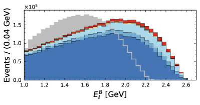
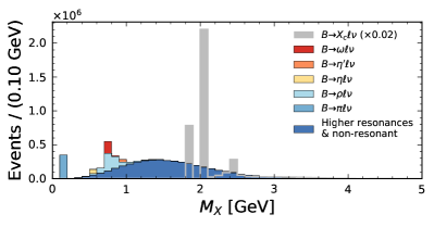
Figure 2: The generator-level $E_{\ell}^{B}$ and $M_{X}$ distributions of the CKM suppressed and favored inclusive semileptonic processes, $B\to X_{u}\,\ell^{+}\,\nu_{\ell}$ (scaled up by a factor of 50) and $B\to X_{c}\,\ell^{+}\,\nu_{\ell}$, respectively, are shown, using the models described in the text.

III Analysis Strategy, Hadronic Tagging, and $X$ Reconstruction

III.1 Neural Network Based Tag Side Reconstruction

We reconstruct collision events using the hadronic full reconstruction algorithm of Ref. Feindt et al. (2011). The algorithm reconstructs one of the $\mathit{{B}{}_{\mspace{-3.0mu}\scriptstyle{}}^{\mspace{-1.0mu}\scriptstyle{}}}$ mesons produced in the collision event using hadronic decay channels. We label such $\mathit{{B}{}_{\mspace{-3.0mu}\scriptstyle{}}^{\mspace{-1.0mu}\scriptstyle{}}}$ mesons in the following as $B_{\mathrm{tag}}$. Instead of attempting to reconstruct as many $\mathit{{B}{}_{\mspace{-3.0mu}\scriptstyle{}}^{\mspace{-1.0mu}\scriptstyle{}}}$ meson decay cascades as possible, the algorithm employs a hierarchical reconstruction ansatz in four stages: at the first stage, neural networks are trained to identify charged tracks and neutral energy depositions as detector stable particles ($e^{+},\mu^{+},K^{+},\pi^{+},\gamma$), neutral $\pi^{0}$ candidates, or $K_{S}^{0}$ candidates. At the second stage, these candidate particles are combined into heavier meson candidates ($J/\psi,D^{0},D^{+},D_{s}$) and for each target final state a neural network is trained to identify probable candidates. In addition to the classifier output from the first stage, vertex fit probabilities of the candidate combinations, and the full four-momentum of the combination are passed to the input layer. At the third stage, candidates for $D^{*\,0},D^{*\,+}$, and $D_{s}^{*}$ mesons are formed and separate neural networks are trained to identify viable combinations. The input layer aggregates the output classifiers from all previous reconstruction stages. The final stage combines the information from all previous stages to form $B_{\mathrm{tag}}$ candidates. The viability of such combinations is again assessed by a neural network that was trained to distinguish correctly reconstructed candidates from wrong combinations and whose output classifier score we denote by $\mathcal{O}_{\mathrm{FR}}$. Over 1104 decay cascades are reconstructed in this manner, achieving an efficiency of 0.28% and 0.18% for charged and neutral $\mathit{{B}{}_{\mspace{-3.0mu}\scriptstyle{}}^{\mspace{-1.0mu}\scriptstyle{}}}$ meson pairs Bevan et al. (e 95), respectively. Finally, the output of this classifier is used as an input and combined with a range of event shape variables to train a neural network to distinguish reconstructed $\mathit{{B}{}_{\mspace{-3.0mu}\scriptstyle{}}^{\mspace{-1.0mu}\scriptstyle{}}}$ meson candidates from continuum processes. The output classifier score of this neural network is denoted as $\mathcal{O}_{\mathrm{Cont}}$. Both classifier scores are mapped to a range of $[0,1)$ signifying the reconstruction quality of poor to excellent candidates. We retain $B_{\mathrm{tag}}$ candidates that show at least moderate agreement based on these two outputs and require that $\mathcal{O}_{\mathrm{FR}}>10^{-4}$ and $\mathcal{O}_{\mathrm{Cont}}>10^{-4}$. Despite these relatively low values, knowledge of the charge and momentum of the decay constituents in combination with the known beam-energy allows one to infer the flavor and four-momentum of the $B_{\mathrm{tag}}$ candidate. We require the $B_{\mathrm{tag}}$ candidates to have at least a beam-constrained mass of

$$M_{\mathrm{bc}}=\sqrt{E_{\mathrm{beam}}^{2}-|\mathbb{p}_{\mathrm{tag}}|^{2}}>5.27\,\text{GeV}\,,$$ (10)

with $\mathbb{p}_{\mathrm{tag}}$ denoting the momentum of the $B_{\mathrm{tag}}$ candidate in the center-of-mass frame of the colliding $e^{+}e^{-}$-pair. Furthermore, $E_{\mathrm{beam}}=\sqrt{s}/2$ denotes half the center-of-mass energy of the colliding $e^{+}e^{-}$-pair. The energy difference

$$\Delta E=E_{\mathrm{tag}}-E_{\mathrm{beam}}\,,$$ (11)

is already used in the input layer of the neural network trained in the final stage of the reconstruction. Here $E_{\mathrm{tag}}$ denotes the energy of the $B_{\mathrm{tag}}$ candidate in the center-of-mass frame of the colliding $e^{+}e^{-}$-pair. In each event a single $B_{\mathrm{tag}}$ candidate is then selected according to the highest $\mathcal{O}_{\mathrm{FR}}$ score of the hierarchical full reconstruction algorithm. All tracks and clusters not used in the reconstruction of the $B_{\mathrm{tag}}$ candidate are used to define the signal side.

III.2 Signal Side Reconstruction

The signal side of the event is reconstructed by identifying a well-reconstructed lepton with $E_{\ell}^{B}=|\mathbb{p}_{\ell}^{B}|>1\,\mathrm{GeV}$ in the signal $B$ rest frame using the likelihood mentioned in Section II. The signal $B$ rest frame is calculated using the momentum of the $B_{\mathrm{tag}}$ candidate via

$$p_{\mathrm{sig}}=p_{e^{+}\,e^{-}}-\left(\sqrt{m_{B}^{2}+|\mathbb{p_{\mathrm{tag}}}|^{2}},\mathbb{p_{\mathrm{tag}}}\right)\,,$$ (12)

with $p_{e^{+}e^{-}}$ denoting the four-momentum of the colliding electron-positron pair. Leptons from $J/\psi$ and photon conversions in detector material are rejected by combining the lepton candidate with oppositely charged tracks ($t$) on the signal side and demanding that $m_{\ell t}>0.14\,\text{GeV}$ and $m_{et}\notin[3.05,3.15]\,\text{GeV}$ or $m_{\mu t}\notin[3.06,3.12]\,\text{GeV}$. If multiple lepton candidates are present on the signal side, the event is discarded as multiple leptons are likely to originate from a double semileptonic $b\to c\to s$ cascade. For charged $B_{\mathrm{tag}}$ candidates, we demand that the charge assignment of the signal-side lepton be opposite that of the $B_{\mathrm{tag}}$ charge. The hadronic $X$ system is reconstructed from the remaining unassigned charged particles and neutral energy depositions. Its four momentum is calculated as

$$p_{X}=\sum_{i}\left(\sqrt{m_{\pi}^{2}+|\mathbb{p}_{i}|^{2}},\mathbb{p}_{i}\right)+\sum_{j}\left(E_{j},\mathbb{k}_{j}\right)\,,$$ (13)

with $E_{i}=|\mathbb{k_{i}}|$ the energy of the neutral energy depositions and all charged particles with momentum $\mathbb{p_{i}}$ are assumed to be pions. With the $X$ system reconstructed, we can also reconstruct the missing mass squared,

$$M_{\mathrm{miss}}^{2}=\left(p_{\mathrm{sig}}-p_{X}-p_{\ell}\right)^{2}\,,$$ (14)

which should peak at zero, $M_{\mathrm{miss}}^{2}\approx m_{\nu}^{2}\approx 0\,\text{GeV}^{2}$, for correctly reconstructed semileptonic $B\to X_{u}\,\ell^{+}\,\nu_{\ell}$ and $B\to X_{c}\,\ell^{+}\,\nu_{\ell}$ decays. The hadronic mass of the $X$ system is later used to discriminate $B\to X_{u}\,\ell^{+}\,\nu_{\ell}$ signal decays from $B\to X_{c}\,\ell^{+}\,\nu_{\ell}$ and other remaining backgrounds. It is reconstructed using

$$M_{X}=\sqrt{\left(p_{X}\right)^{\mu}\left(p_{X}\right)_{\mu}}\,.$$ (15)

In addition, we reconstruct the four-momentum-transfer squared, $q^{2}$, as

$$q^{2}=\left(p_{\mathrm{sig}}-p_{X}\right)^{2}\,.$$ (16)

The resolution of both variables for $B\to X_{u}\,\ell^{+}\,\nu_{\ell}$ is shown in Figure 3 as residuals with respect to the generated values of $q^{2}$ and $M_{X}$. The resolution for $M_{X}$ has a root-mean-square (RMS) deviation of $0.47\,\text{GeV}$, but exhibits a large tail towards larger values. The distinct peak at 0 is from $B^{0}\to\pi^{-}\,\ell^{+}\,\nu_{\ell}$ and other low-multiplicity final states comprised of only charged pions. The four-momentum-transfer squared $q^{2}$ exhibits a large resolution, which is caused by a combination of the tag-side $B$ and the $X$ reconstruction. The RMS deviation for $q^{2}$ is $1.59\,\text{GeV}^{2}$. The core resolution is dominated by the tagging resolution, whereas the large negative tail is dominated from the resolution of the reconstruction of the $X$ system.

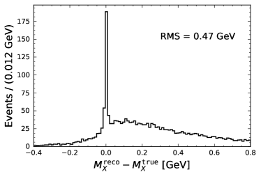
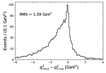
Figure 3: The resolution of the reconstructed $M_{X}$ and $q^{2}$ values for $B\to X_{u}\,\ell^{+}\,\nu_{\ell}$ signal is shown as a residual with respect to the generated values.

III.3 Background Suppression BDT

At this point in the reconstruction, the $B\to X_{c}\,\ell^{+}\,\nu_{\ell}$ process completely dominates the selected events. To identify $B\to X_{u}\,\ell^{+}\,\nu_{\ell}$, we combine several distinguishing features into a single discriminant. This is achieved by using a machine learning based classification with boosted decision trees (BDTs). Note that all momenta are in the center-of-mass frame of the colliding $e^{+}e^{-}$-pair. These features are:

1. $M_{\mathrm{miss}}^{2}$: The average $B\to X_{c}\,\ell^{+}\,\nu_{\ell}$ multiplicity is higher than $B\to X_{u}\,\ell^{+}\,\nu_{\ell}$, broadening the missing mass squared distribution.

2. $D^{*}$ veto: We search for low momentum neutral and charged pions in the $X$ system with $|\mathbb{p}_{\pi}|<220$ MeV, compatible with a $D^{*}\to D\pi$ transition. The key idea of this is that due to the small available phase space from the small mass difference between the $D^{*}$ and $D$ mesons, the flight direction of the slow pion is strongly correlated with the $D^{*}$ momentum direction. The energy and momentum of a $D^{*}$ candidate can thus be approximated as

   $$E_{D^{*}} =\frac{m_{D^{*}}}{m_{D^{*}}-m_{D}}\times E_{\pi}\,,$$

   $$\mathbb{p}_{D^{*}} =\mathbb{p_{\pi}}\times\frac{\sqrt{E_{D^{*}}^{2}-m_{D^{*}}^{2}}}{|\mathbb{p}_{\pi}|}\,,$$ (17)

   with $m_{D^{*}}$ and $m_{D}$ denoting the $D^{*}$ and $D$ meson masses, respectively, and $E_{\pi}=\sqrt{m_{\pi}^{2}+|\mathbb{p}_{\pi}|^{2}}$ is the energy of the slow pion. Using the $D^{*}$ candidate four momentum $p_{D^{*}}=(E_{D^{*}},\mathbb{p}_{D^{*}})$ we can calculate

   $$M_{\mathrm{miss},D^{*}}^{2} =\left(p_{\mathrm{sig}}-p_{D^{*}}-p_{\ell}\right)^{2}\,,$$

   $$\cos\theta_{B,D^{*}\ell} =\frac{2E_{\mathrm{beam}}E_{D^{*}\ell}-m_{B}^{2}-m_{D^{*}\ell}^{2}}{2|\mathbb{p}_{B}||\mathbb{p}_{D^{*}\ell}|}\,,$$

   $$\cos\theta^{*} =\frac{\mathbb{p}_{\ell}\cdot\mathbb{p}_{D^{*}}}{|\mathbb{p}_{\ell}||\mathbb{p}_{D^{*}}|}\,,$$ (18)

   with $p_{D^{*}\ell}=p_{D^{*}}+p_{\ell}=(E_{D^{*}\ell},\mathbb{p}_{D^{*}\ell})$ and $|\mathbb{p}_{B}|=\sqrt{E_{B}^{2}-m_{B}^{2}}$. These three variables are used exclusively for events with charged and neutral slow pion candidates.

3. Kaons: We identify the number of $K^{+}$ candidates using the particle-identification likelihood, cf. Section II. In addition, we reconstruct $K_{S}^{0}$ candidates from displaced tracks found in the $X$ system.

4. $B_{\mathrm{sig}}$ vertex fit: The charmed mesons produced in $B\to X_{c}\,\ell^{+}\,\nu_{\ell}$ transitions exhibit a longer lifetime than their charmless counterparts produced in $B\to X_{u}\,\ell^{+}\,\nu_{\ell}$ decays. This can be exploited by carrying out a vertex fit using the lepton and all charged constituents, not identified as kaons, of the $X$ system and we use its $\chi^{2}$ value as a discriminator.

5. $Q_{\mathrm{tot}}$: The total event charge as calculated from the $X$ system plus lepton on the signal and from the $B_{\mathrm{tag}}$ constituents. Due to the larger average multiplicity of $B\to X_{c}\,\ell^{+}\,\nu_{\ell}$, the expected net zero event charge is more often violated in comparison to $B\to X_{u}\,\ell^{+}\,\nu_{\ell}$ candidate events.

We use the BDT implementation of Ref. Chen and Guestrin (2016) and train a classifier $\mathcal{O}_{\mathrm{BDT}}$ with simulated $B\to X_{u}\,\ell^{+}\,\nu_{\ell}$ and $B\to X_{c}\,\ell^{+}\,\nu_{\ell}$ events, which we discard in the later analysis. Ref. Chen and Guestrin (2016) uses optimized boosting and pruning procedures to maximize the classification performance. We choose a selection criteria on $\mathcal{O}_{\mathrm{BDT}}$ that rejects 98.7% of $B\to X_{c}\,\ell^{+}\,\nu_{\ell}$ and retains 18.5% of $B\to X_{u}\,\ell^{+}\,\nu_{\ell}$ signal. This working point was chosen by maximizing the significance of the most inclusive partial branching fraction, taking into account the full set of systematic uncertainties and the full analysis procedure. The stability of the result as a function of the BDT selection is further discussed in Section VIII.

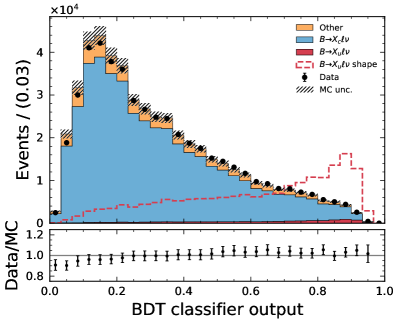
Figure 4: The shape of the background suppression classifier $\mathcal{O}_{\mathrm{BDT}}$ is shown. MC is divided into $B\to X_{u}\,\ell^{+}\,\nu_{\ell}$ signal, the dominant $B\to X_{c}\,\ell^{+}\,\nu_{\ell}$ background, and all other contributions. To increase visibility, the $B\to X_{u}\,\ell^{+}\,\nu_{\ell}$ component is shown with a scaling factor (red dashed line). The uncertainties on the MC contain the full systematic errors and are further discussed in Section V.

Table 2 lists the efficiencies for signal and $B\to X_{c}\,\ell^{+}\,\nu_{\ell}$ background for the $M_{\mathrm{bc}}$ and the BDT selections. Figure 4 shows the output classifier of the background suppression BDT for MC and data. The classifier output shows good agreement between simulated and observed data, with the exception of the first two signal depleted bins. A comparison of the shape of all input variables for $B\to X_{u}\,\ell^{+}\,\nu_{\ell}$ and $B\to X_{c}\,\ell^{+}\,\nu_{\ell}$, and further MC and data comparisons can be found in Appendix B.

Table 2: The selection efficiencies for $B\to X_{u}\,\ell^{+}\,\nu_{\ell}$ signal, $B\to X_{c}\,\ell^{+}\,\nu_{\ell}$   and for data are listed after the reconstruction of the $B_{\mathrm{tag}}$ and lepton candidate. The nominal selection requirement on the BDT classifier $\mathcal{O}_{\mathrm{BDT}}$ is 0.85. The other two requirements were introduced to test the stability of the result, cf. Section VIII.

Selection	$B\to X_{u}\,\ell^{+}\,\nu_{\ell}$	$B\to X_{c}\,\ell^{+}\,\nu_{\ell}$	Data
$M_{\mathrm{bc}}>5.27\,\text{GeV}$	84.8%	83.8%	80.2%
$\mathcal{O}_{\mathrm{BDT}}>0.85$	18.5%	1.3%	1.6%
$\mathcal{O}_{\mathrm{BDT}}>0.83$	21.9%	1.7%	2.1%
$\mathcal{O}_{\mathrm{BDT}}>0.87$	14.5%	0.9%	1.1%

III.4 Tagging Efficiency Calibration

The reconstruction efficiency of the hadronic full reconstruction algorithm of Ref. Feindt et al. (2011) differs between simulated samples and the reconstructed data. This difference mainly arises due to imperfections, e.g. in the simulation of detector responses, particle identification efficiencies, or incorrect branching fractions in the reconstructed decay cascades. To address this, the reconstruction efficiency is calibrated using a data-driven approach and we follow closely the procedure outlined in Ref. Glattauer et al. (2016). We reconstruct full reconstruction events by requiring exactly one lepton on the signal side, and apply the same $B_{\mathrm{tag}}$ and lepton selection criteria outlined in the previous section. This $B\to X\,\ell^{+}\,\nu_{\ell}$ enriched sample is divided into groups of subsamples according to the $B_{\mathrm{tag}}$ decay channel and the multivariate classifier output $\mathcal{O}_{\mathrm{FR}}$ used in the hierarchical reconstruction. Each of these groups of subsamples is studied individually to derive a calibration factor for the hadronic tagging efficiency: the calibration factor is obtained by comparing the number of inclusive semileptonic $B$-meson decays, $N(B\to X\,\ell^{+}\,\nu_{\ell})$, in data with the expectation from the simulated samples, $N^{\mathrm{MC}}(B\to X\,\ell^{+}\,\nu_{\ell})$. The semileptonic yield is determined via a binned maximum likelihood fit using the the lepton energy spectrum. To reduce the modeling dependence of the $B\to X\,\ell^{+}\,\nu_{\ell}$ sample this is done in a coarse granularity of five bins. The calibration factor of each these groups of subsamples is given by

$$C_{\mathrm{tag}}(B_{\mathrm{tag}}\,\text{mode},\mathcal{O}_{\mathrm{FR}}) =\frac{N(B\to X\,\ell^{+}\,\nu_{\ell})}{N^{\mathrm{MC}}(B\to X\,\ell^{+}\,\nu_{\ell})}\,.$$ (19)

The free parameters in the fit are the yield of the semileptonic $B\to X\,\ell^{+}\,\nu_{\ell}$ decays, the yield of backgrounds from fake leptons and the yield of backgrounds from true leptons. Approximately 1200 calibration factors are determined this way. The leading uncertainty on the $C_{\mathrm{tag}}$ factors is from the assumed $B\to X\,\ell^{+}\,\nu_{\ell}$ composition and the lepton PID performance, cf. Section V. We also apply corrections to the continuum efficiency. These are derived by using the off-resonance sample and comparing the number of reconstructed off-resonance events in data with the simulated on-resonance continuum events, correcting for differences in the selection.

IV Fitting Procedure

Table 3: The binning choices of the five fit scenarios are given.

Fit variable	Bins
$M_{X}$	$[0,1.5,1.9,2.5,3.1,4.0]\,\text{GeV}$
$q^{2}$	$[0,2,4,6,8,10,12,14,26]\,\text{GeV}^{2}$
$E_{\ell}^{B}$	15 equidist. bins in $[1,2.5]\,\text{GeV}$ & $[2.5,2.7]\,\text{GeV}$
$M_{X}:q^{2}$	$[0,1.5]\,\text{GeV}$ $\times[0,2,4,6,8,10,12,14,26]\,\text{GeV}^{2}$
	$[1.5,1.9]\,\text{GeV}$ $\times[0,2,4,6,26]\,\text{GeV}^{2}$
	$[1.9,2.5]\,\text{GeV}$ $\times[0,2,4,26]\,\text{GeV}^{2}$
	$[2.5,4.0]\,\text{GeV}$ $\times[0,2,26]\,\text{GeV}^{2}$

After the selection, we retain 9875 events. In order to determine the $B\to X_{u}\,\ell^{+}\,\nu_{\ell}$ signal yield and constrain all backgrounds, we perform a binned likelihood fit of these events in several discriminating variables. To reduce the dependence on the precise modeling of the $B\to X_{u}\,\ell^{+}\,\nu_{\ell}$ signal, we use coarse bins over regions that are very sensitive to the admixture of resonant and non-resonant decays, cf. Section II, and explore different variables for the signal extraction. The total likelihood function is constructed as the product of individual Poisson distributions $\mathcal{P}$,

$$\mathcal{L}=\prod_{i}^{\rm bins}\,\mathcal{P}\left(n_{i};\nu_{i}\right)\,\times\prod_{k}\,\mathcal{G}_{k}\,,$$ (20)

with $n_{i}$ denoting the number of observed data events and $\nu_{i}$ the total number of expected events in a given bin $i$. Here, $\mathcal{G}_{k}$ are nuisance-parameter (NP) constraints, whose role is to incorporate systematic uncertainties of a source $k$ into the fit. Their construction is further discussed in Section V. The number of expected events in a given bin, $\nu_{i}$, is estimated using simulated collision events and is given by

$$\nu_{i}=\sum_{k}^{\mathrm{component}}\,f_{ik}\,\eta_{k}\,,$$ (21)

with $\eta_{k}$ denoting the total number of events from a given fit component $k$, and $f_{ik}$ denoting the fraction of such events being reconstructed in bin $i$ as determined by the MC simulation. The three fit components we determine are:

• Signal $B\to X_{u}\,\ell^{+}\,\nu_{\ell}$ events that fall inside a phase-space region for a partial branching fraction we wish to determine.

• Signal $B\to X_{u}\,\ell^{+}\,\nu_{\ell}$ events that fall outside said region if applicable. This component can have very similar shapes as other backgrounds. We thus constrain this component in all fits to its expectation using the world average of $\mathcal{B}(B\to X_{u}\,\ell^{+}\,\nu_{\ell})=\left(2.13\pm 0.30\right)\times 10^{-3}$ Zyla et al. (2020c). We also investigated different approaches: for instance linking this component with the component of a). This leads to small shifts of $\mathcal{O}(0.3-1\%)$ of the reported partial branching fractions using this component.

• Background events; such are dominated by $B\to X_{c}\,\ell^{+}\,\nu_{\ell}$ and other decays that produce leptons in the final state (e.g. from $B\to h_{1}h_{2}$ and $h_{2}\to h_{3}\ell^{-}\nu$ with $h_{1},h_{2}$, and $h_{3}$ denoting hadronic final states). Other contributions are from misidentified lepton candidates and a small amount of continuum processes. A full description of all background processes is given in Section III.

We carry out five separate fits to measure three partial branching fractions, using different discriminating variables to determine the $B\to X_{u}\,\ell^{+}\,\nu_{\ell}$ yield. The fits and variables are:

1. The hadronic mass, $M_{X}$: Signal is expected to pre-dominantly populate the low hadronic mass region, whereas remaining $B\to X_{c}\,\ell^{+}\,\nu_{\ell}$ background will produce a sharp peak at around $M_{X}\approx 2\,\text{GeV}$. The sizeable resolution on the reconstruction of the $X$ system will result in a non-negligible amount of these backgrounds to also be present in the low and high $M_{X}$ region. The determined signal yields are used to measure the partial branching fraction of $M_{X}<1.7\,\mathrm{GeV}$ and $E_{\ell}^{B}>1\,\text{GeV}$. We thus use two signal templates and split events according to generator-level $M_{X}<1.7\,\mathrm{GeV}$ and $M_{X}>1.7\,\mathrm{GeV}$.

2. The four-momentum-transfer squared, $q^{2}$: Signal will on average have a higher $q^{2}$ than $B\to X_{c}\,\ell^{+}\,\nu_{\ell}$ background, whose kinematic endpoint is $q^{2}=\left(m_{B}-m_{D}\right)^{2}\approx 11.6\,\text{GeV}^{2}$. However, the reconstructed $q^{2}$ of $B\to X_{c}\,\ell^{+}\,\nu_{\ell}$ events is smeared over the entire kinematic range due to the sizeable resolution in the reconstruction of the inclusive $X$ system and the $B_{\mathrm{tag}}$ reconstruction. To reduce background from $B\to X_{c}\,\ell^{+}\,\nu_{\ell}$ events, we apply a cut on the reconstructed $M_{X}$ and require a value smaller than $1.7\,\mathrm{GeV}$. The determined signal yields are used to measure the partial branching fraction of $M_{X}<1.7\,\mathrm{GeV}$, $q^{2}>8\,\mathrm{GeV}^{2}$, and $E_{\ell}^{B}>1\,\text{GeV}$. We use two signal templates: Template a) is defined as signal events with generator-level values of $M_{X}<1.7\,\mathrm{GeV}$ and $q^{2}>8\,\mathrm{GeV}^{2}$ and template b) contains all other signal events.

3. The lepton energy in the $B$ meson rest-frame, $E_{\ell}^{B}$: Signal and $B\to X_{c}\,\ell^{+}\,\nu_{\ell}$ can be separated beyond the kinematic endpoint of the $B\to X_{c}\,\ell^{+}\,\nu_{\ell}$ background, which is $\frac{1}{2m_{B}}\left(m_{B}^{2}-m_{D}^{2}+m_{\ell}^{2}\right)\approx 2.3\,\text{GeV}$. The lepton energy is reconstructed using its momentum ($E_{\ell}^{B}=|\mathbb{p}_{\ell}^{B}|$), which has excellent resolution. This makes the measurement more sensitive to the exact composition of the $B\to X_{c}\,\ell^{+}\,\nu_{\ell}$ background and $B\to X_{u}\,\ell^{+}\,\nu_{\ell}$ signal. To minimize the dependence on the signal modeling, the endpoint of the lepton spectrum, ranging from $E_{\ell}^{B}\in[2.5,2.7]\,\text{GeV}$, is treated as a single coarse bin in the fit. To reduce the dependence on the exact modeling of $B\to X_{c}\,\ell^{+}\,\nu_{\ell}$   we require $M_{X}<1.7$   GeV. The determined signal yields are used to measure the partial branching fraction with $M_{X}<1.7\,\mathrm{GeV}$ and the signal templates are split accordingly into a matching generator-level template and all other signal events.

4. The next fit also analyzes $E_{\ell}^{B}$, but uses the determined signal yields to measure the partial branching fraction with $E_{\ell}^{B}>1\,\text{GeV}$. Thus no separation of signal events in different categories is used.

5. The final fit uses $M_{X}$ and $q^{2}$ simultaneously in a two dimensional fit ($M_{X}:q^{2}$). This fit also measure the partial branching fraction with $E_{\ell}^{B}>1\,\text{GeV}$ and no separation into different categories of signal events is used.

A summary of the binning choices of the kinematic variables is provided in Table 3 and we further remove events with $M_{X}>4\,\mathrm{GeV}$ in all fits. Further, we also exclude events with negative $q^{2}$ values in the $M_{X}$, $M_{X}:q^{2}$, and $q^{2}$ fits. The likelihood Eq. 20 is numerically maximized to fit the value of the different components, $\eta_{k}$, from the observed events and by using the sequential least squares programming method implementation of Ref. Ongmongkolkul et al. (12). Confidence intervals are constructed using the profile likelihood ratio method. For a given component $\eta_{k}$ the ratio is

$$\Lambda(\eta_{k})=-2\ln\frac{\mathcal{L}(\eta_{k},\boldsymbol{\widehat{\eta}_{\eta_{k}}},\boldsymbol{\widehat{\theta}_{\eta_{k}}})}{\mathcal{L}(\widehat{\eta}_{k},\boldsymbol{\widehat{\eta}},\boldsymbol{\widehat{\theta}})}\,,$$ (22)

where $\widehat{\eta}_{k}$, $\boldsymbol{\widehat{\eta}}$, $\boldsymbol{\widehat{\theta}}$ are the values of the component of interest, the remaining components, and a vector of nuisance parameters (NPs), respectively, that maximize the likelihood function, whereas the remaining components $\boldsymbol{\widehat{\eta}_{\eta_{k}}}$ and nuisance parameters $\boldsymbol{\widehat{\theta}_{\eta_{k}}}$ maximize the likelihood for the specific value $\eta_{k}$. In the asymptotic limit, the test statistic Eq. 22 can be used to construct approximate confidence intervals through

$$1-\text{CL}=\int_{\Lambda(\eta_{k})}^{\infty}\,f_{\chi^{2}}(x;1\,\text{dof})\,\text{d}x\,,$$ (23)

with $f_{\chi^{2}}(x;1\,\text{dof})$ denoting the $\chi^{2}$ distribution of the variable $x$ with a single degree of freedom. Further, CL denotes the desired confidence level. The determined signal yields $\widehat{\eta}_{k}=\widehat{\eta}_{\mathrm{sig}}$ are translated into partial branching fractions via

$$\Delta\mathcal{B}(B\to X_{u}\,\ell^{+}\,\nu_{\ell};\mathrm{Reg.}) =\frac{\widehat{\eta}_{\mathrm{sig}}\cdot\epsilon_{\Delta\mathcal{B}(\mathrm{Reg.})}}{4\left(\epsilon_{\mathrm{tag}}\cdot\epsilon_{\mathrm{sel}}\right)\cdot N_{BB}}\,.$$ (24)

Here $\epsilon_{\mathrm{tag}}$ denotes the tagging efficiency, as determined after applying the calibration factor introduced in Section III.4. Further, $\epsilon_{\mathrm{sel}}$ and $\epsilon_{\Delta\mathcal{B}(\text{Reg.})}$ denote the signal side selection efficiency and a correction to the efficiency to account for the fraction of $B\to X_{u}\,\ell^{+}\,\nu_{\ell}$ phase-space region that is measured. The factor of $4$ in the denominator is due to the factor $N_{BB}=\left(771.58\pm 9.78\right)\times 10^{6}$ $B$ meson pairs and our averaging over electron and muon final states.

To validate the fit procedure we generated ensembles of pseudoexperiments for different input branching fractions for $B\to X_{u}\,\ell^{+}\,\nu_{\ell}$ signal and $B\to X_{c}\,\ell^{+}\,\nu_{\ell}$ background. Fits to these ensembles show no biases in central values and no under- or overcoverage of CI. Using the current world average of $\mathcal{B}(B\to X_{u}\,\ell^{+}\,\nu_{\ell})=\left(2.13\pm 0.30\right)\times 10^{-3}$, we expect approximately between 930 - 2070 $B\to X_{u}\,\ell^{+}\,\nu_{\ell}$ signal events with significances $s=\widehat{\eta}_{\mathrm{sig}}/\epsilon$ ranging from about 9 to 15 standard deviations, depending on the signal region under study, and with $\epsilon$ being the expected fit error determined from Asimov data sets Cowan et al. (2011).

V Systematic Uncertainties

Several systematic uncertainties affect the determination of the reported partial branching fractions. The most important uncertainties arise from the modeling of the $B\to X_{u}\,\ell^{+}\,\nu_{\ell}$ signal component and from the tagging calibration correction. This is followed by uncertainties on particle identification of kaons and leptons, the uncertainty on the number of $B$-meson pairs, the statistical uncertainty on the used MC samples, and uncertainties related to the efficiency of the track reconstructions. Table 4 summarizes the systematic uncertainties for the five measured partial branching fractions probing three phase-space regions. The table separates uncertainties that originate from the background subtraction ( ‘Additive uncertainties’) and uncertainties related to the translation of the fitted signal yields into partial branching fractions ( ‘Multiplicative uncertainties’).

The tagging calibration uncertainties are evaluated by producing different sets of calibration factors. These sets take into account the correlation structure from common systematic uncertainties (cf. Section  III.4) and that individual channels and ranges of the output classifier are statistically independent. When applying the different sets of calibration factors, we notice only negligible shape changes on the signal and background template shapes, but the overall tagging efficiency is affected. The associated uncertainty on the calibration factors is found to be 3.6% and is identical for the five measured partial branching fractions. The $B\to X_{u}\,\ell^{+}\,\nu_{\ell}$ and $B\to X_{c}\,\ell^{+}\,\nu_{\ell}$ modeling uncertainties do directly affect the shapes of $M_{X}$, $q^{2}$, and $E_{\ell}^{B}$ signal and background distributions. Further, the $B\to X_{u}\,\ell^{+}\,\nu_{\ell}$ modeling affects the overall reconstruction efficiencies and migrations of events inside and outside of the phase-space regions we measure. We evaluate the uncertainties on the composition of the hybrid $B\to X_{u}\,\ell^{+}\,\nu_{\ell}$ MC by variations of the $B\to\pi\,\ell^{+}\,\nu_{\ell}$, $B\to\rho\,\ell^{+}\,\nu_{\ell}$, $B\to\omega\,\ell^{+}\,\nu_{\ell}$, $B\to\eta\,\ell^{+}\,\nu_{\ell}$, $B\to\eta^{\prime}\,\ell^{+}\,\nu_{\ell}$ branching fractions and form factors. The uncertainty on non-resonant $B\to X_{u}\,\ell^{+}\,\nu_{\ell}$ contributions in the hybrid model is estimated by changing the underlying model from that of DFN De Fazio and Neubert (1999) to that of BLNP Lange et al. (2005a). In addition, the uncertainty on the used DFN parameters $m_{b}^{1S}$ and $a$ (cf. Section II) are incorporated. For each of these variations, new hybrid weights are calculated to propagate the uncertainties into shapes and efficiencies. We estimate the uncertainties of $X_{u}$ fragmentation into $s\bar{s}$ quark pairs by variations of the corresponding JETSET parameter $\gamma_{s}$ (cf. Ref. T. Sjöstrand (1994)). As our BDT is trained to reject final states with kaon candidates, a change in this fraction will directly impact the signal efficiency. The $s\bar{s}$ production probability has been measured by Refs. Althoff et al. (1985); Bartel et al. (1983) at center-of-mass energies of 12 and 36 GeV with values of $\gamma_{s}=0.35\pm 0.05$ and $\gamma_{s}=0.27\pm 0.06$, respectively. We adopt the value and error of $\gamma_{s}=0.30\pm 0.09$, which spans the range of both measurements including their uncertainties. The $X_{u}$ system of the non-resonant signal component is hadronized by JETSET into final states with two or more pions. We test the impact on the signal efficiency by changing the post-fit charged pion multiplicity of non-resonant $B\to X_{u}\,\ell^{+}\,\nu_{\ell}$ to the distribution observed in data in the signal enriched region of $M_{X}<1.7$ GeV (cf. Section VIII.5 and Appendix C). The $B\to X_{c}\,\ell^{+}\,\nu_{\ell}$ background after the BDT selection is dominated by $B\to D\,\ell^{+}\,\nu_{\ell}$ and $B\to D^{*}\,\ell^{+}\,\nu_{\ell}$ decays. We evaluate the uncertainties on the modeling of $B\to D\,\ell^{+}\,\nu_{\ell}$   $B\to D^{*}\,\ell^{+}\,\nu_{\ell}$   and $B\to D^{**}\,\ell^{+}\,\nu_{\ell}$ by variations of the BGL parameters and heavy quark form factors within their uncertainties. In addition, we propagate the branching fraction uncertainties. The uncertainties on the $B\to X_{c}\,\ell^{+}\,\nu_{\ell}$ gap branching fractions are taken to be large enough to account for the difference between the sum of all exclusive branching fractions measured and the inclusive branching fraction measured. We also evaluate the impact on the efficiency of the lepton- and hadron-identification uncertainties, and the overall tracking efficiency uncertainty. The statistical uncertainty on all generated MC samples is also evaluated and propagated into the systematic errors.

We incorporate the effect of additive systematic uncertainties directly into the likelihood function. This can be done by introducing a vector of NPs, $\boldsymbol{\theta}_{k}$, for each fit template of a process $k$ (e.g. signal or background). Each element of this vector represents one bin of the fitted observables of interest (e.g. $M_{X}$,$q^{2}$, $E_{\ell}^{B}$ or a 2D bin of $M_{X}:q^{2}$). These NPs are constrained parameters in the likelihood Eq. 20 using multivariate Gaussian distributions, $\mathcal{G}_{k}=\mathcal{G}_{k}(\boldsymbol{0};\boldsymbol{\theta}_{k},\Sigma_{k})$. Here $\Sigma_{k}$ denotes the systematic covariance matrix for a given template $k$ and $\boldsymbol{\theta}_{k}$ is a vector of NPs. The covariance $\Sigma_{k}$ is the sum over all possible uncertainty sources for a given template $k$,

$$\Sigma_{k}=\sum_{s}^{\text{error sources}}\Sigma_{ks}\,,$$ (25)

with $\Sigma_{ks}$ denoting the covariance matrix of error source $s$. The covariance matrices $\Sigma_{ks}$ depend on uncertainty vectors $\boldsymbol{\sigma_{ks}}$, which represent the absolute error in bins of the fit variable of template $k$. Uncertainties from the same error source are either fully correlated, or for the case of MC or other statistical uncertainties, are treated as uncorrelated. Both cases can be expressed as $\Sigma_{ks}=\boldsymbol{\sigma_{ks}}\otimes\boldsymbol{\sigma_{ks}}$ or $\Sigma_{ks}=\text{Diag}\left(\boldsymbol{\sigma_{ks}}^{2}\right)$, respectively. For particle identification uncertainties, we estimate $\Sigma_{ks}$ using sets of correction tables, sampled according to their statistical and systematic uncertainties. The systematic NPs are incorporated in Eq. 21 by rewriting the fractions $f_{ik}$ for all templates as

$$f_{ik}=\frac{\eta_{ik}^{\rm MC}}{\sum_{j}\eta_{jk}^{\rm MC}}\to\frac{\eta_{ik}^{\rm MC}\left(1+\theta_{ik}\right)}{\sum_{j}\eta_{jk}^{\rm MC}\left(1+\theta_{jk}\right)},$$ (26)

to take into account changes in the signal or background shape. Here $\eta_{ik}^{\rm MC}$ denotes the predicted number of MC events of a given bin $i$ and a process $k$, and $\theta_{ik}$ is the associated nuisance parameter constrained by $\mathcal{G}_{k}$.

VI $B\to X_{c}\ell\bar{\nu}_{\ell}$ Control Region

Figure 5 compares the reconstructed $M_{X}$, $q^{2}$, and $E_{\ell}^{B}$ distributions with the expectation from MC before applying the background suppression BDT. All corrections are applied and the MC uncertainty contains all systematic uncertainties discussed in Section V. The agreement of $M_{X}$ and $q^{2}$ is excellent, but some differences in the shape of the lepton momentum spectrum are seen. This is likely due to imperfections of the modeling of the inclusive $B\to X_{c}\,\ell^{+}\,\nu_{\ell}$ background. The discrepancy reduces in the $M_{X}<1.7$ GeV region. The main results of this paper will be produced by fitting $q^{2}$ and $M_{X}$ in two dimensions. We use the lepton spectrum to measure the same regions of phase space, to validate the obtained results.

VII $B\to X_{u}\,\ell^{+}\,\nu_{\ell}$ Signal Region

Figure 6 shows the reconstructed $M_{X}$, $q^{2}$, and $E_{\ell}^{B}$ distributions after the BDT selection is applied. The $B\to X_{u}\,\ell^{+}\,\nu_{\ell}$ contribution is now clearly visible at low $M_{X}$ and high $E_{\ell}^{B}$, while the reconstructed events and the MC expectation show good agreement. The $B\to X_{c}\,\ell^{+}\,\nu_{\ell}$ background is dominated by contributions from $B\to D\,\ell^{+}\,\nu_{\ell}$ and $B\to D^{*}\,\ell^{+}\,\nu_{\ell}$ decays, and the remaining background is predominantly from secondary leptons, and misidentified lepton candidates.

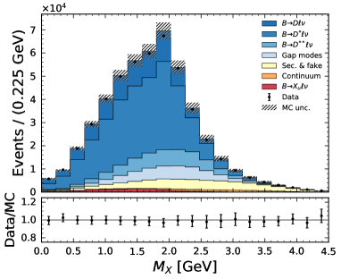
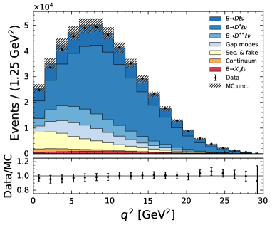
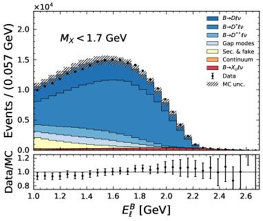
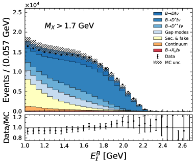
Figure 5: (Top) The $M_{X}$ and $q^{2}$ spectra of the selected candidates prior to applying the background BDT are shown.
(Bottom) The $E_{\ell}^{B}$ spectrum of the selected candidates prior to applying the background BDT are shown for events with $M_{X}<1.7$ GeV and $M_{X}>1.7$ GeV.

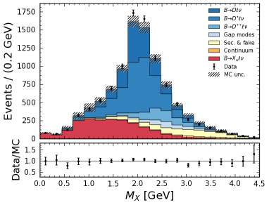
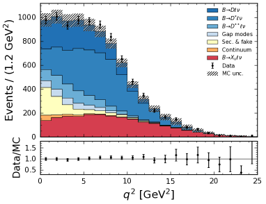
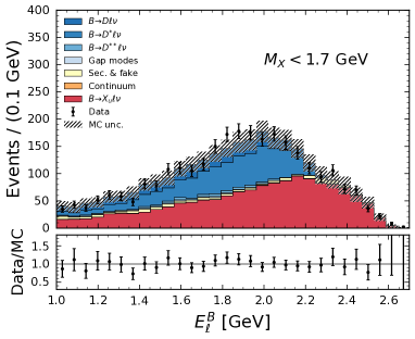
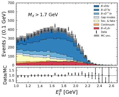
Figure 6: The $M_{X}$, $q^{2}$ and $E_{\ell}^{B}$ spectra after applying the background BDT but before the fit are shown. The $B\to X_{u}\,\ell^{+}\,\nu_{\ell}$ contribution is shown in red and scaled to the world average of $\mathcal{B}(B\to X_{u}\,\ell^{+}\,\nu_{\ell})=\left(2.13\pm 0.30\right)\times 10^{-3}$. The data and MC agreement is reasonable in all variables. The $E_{\ell}^{B}$ spectra is shown with selections of $M_{X}<1.7\,\text{GeV}$ and $M_{X}>1.7\,\text{GeV}$. The cut of $M_{X}<1.7\,\text{GeV}$ is later used in the fit to reduce the dependence on the $B\to X_{c}\,\ell^{+}\,\nu_{\ell}$ modeling of higher charmed states.

Table 4: The relative uncertainty on the extracted $B\to X_{u}\,\ell^{+}\,\nu_{\ell}$ partial branching fractions are shown. For definitions of additive and multiplicative errors, see text.

	Relative uncertainties [%]
Phase-space region	$M_{X}<1.7\,\mathrm{GeV}$,	$M_{X}<1.7\,\mathrm{GeV},$	$M_{X}<1.7\,\mathrm{GeV},$	$E_{\ell}^{B}>1\,\mathrm{GeV}$	$E_{\ell}^{B}>1\,\mathrm{GeV}$
	$E_{\ell}^{B}>1\,\mathrm{GeV}$	$E_{\ell}^{B}>1\,\mathrm{GeV}$	$q^{2}>8\,\text{GeV}^{2},$
			$E_{\ell}^{B}>1\,\mathrm{GeV}$
Fit variable(s)	($M_{X}$ fit)	($E_{\ell}^{B}$ fit)	($q^{2}$ fit)	($E_{\ell}^{B}$ fit)	($M_{X}:q^{2}$ fit)
Additive uncertainties
$B\to X_{u}\,\ell^{+}\,\nu_{\ell}$ modeling
$B\to\pi\,\ell^{+}\,\nu_{\ell}$ FFs	0.1	0.7	1.4	0.6	0.4
$B\to\rho\,\ell^{+}\,\nu_{\ell}$ FFs	0.2	1.9	4.3	1.9	0.7
$B\to\omega\,\ell^{+}\,\nu_{\ell}$ FFs	0.5	3.2	5.2	3.1	0.8
$B\to\eta\,\ell^{+}\,\nu_{\ell}$ FFs	0.1	1.6	3.0	1.6	0.3
$B\to\eta^{\prime}\,\ell^{+}\,\nu_{\ell}$ FFs	0.1	1.6	3.0	1.6	1.6
$\mathcal{B}(B\to\pi\,\ell^{+}\,\nu_{\ell})$	0.2	0.1	0.2	0.1	0.2
$\mathcal{B}(B\to\rho\,\ell^{+}\,\nu_{\ell})$	0.3	0.7	0.8	0.5	0.4
$\mathcal{B}(B\to\omega\,\ell^{+}\,\nu_{\ell})$	$<$0.1	0.1	0.8	0.1	0.1
$\mathcal{B}(B\to\eta\,\ell^{+}\,\nu_{\ell})$	$<$0.1	0.1	$<$0.1	0.1	$<$0.1
$\mathcal{B}(B\to\eta^{\prime}\,\ell^{+}\,\nu_{\ell})$	$<$0.1	$<$0.1	0.1	0.1	$<$0.1
$\mathcal{B}(B\to X_{u}\,\ell^{+}\,\nu)$	0.7	2.0	2.1	2.1	2.1
DFN parameters	2.3	3.5	1.1	3.5	5.0
Hybrid model	2.7	8.7	4.6	8.7	3.1
$B\to X_{c}\,\ell^{+}\,\nu_{\ell}$ modeling
$B\to D\,\ell^{+}\,\nu_{\ell}$ FFs	0.1	0.1	0.9	0.1	$<$0.1
$B\to D^{*}\,\ell^{+}\,\nu_{\ell}$ FFs	1.4	1.2	3.0	1.3	1.1
$B\to D^{**}\,\ell^{+}\,\nu_{\ell}$ FFs	0.4	0.5	0.3	0.5	0.4
$\mathcal{B}(B\to D\,\ell^{+}\,\nu_{\ell})$	0.1	$<$0.1	0.2	$<$0.1	0.2
$\mathcal{B}(B\to D^{*}\,\ell^{+}\,\nu_{\ell})$	$<$0.1	$<$0.1	0.3	$<$0.1	0.2
$\mathcal{B}(B\to D^{**}\,\ell^{+}\,\nu_{\ell})$	0.6	0.1	0.3	0.1	0.5
Gap modeling	1.1	0.1	0.3	0.1	1.0
MC statistics	1.3	1.6	3.8	1.7	1.6
Tracking efficiency	0.3	-	0.8	-	0.4
$\mathcal{L}_{\rm\ell ID}$ shape	1.0	0.5	1.3	0.6	1.2
$\mathcal{L}_{\rm K/\pi ID}$ shape	1.2	-	1.3	-	1.0
$D\to X\ell\,\nu_{\ell}$	0.1	0.1	0.1	0.1	0.1
$\pi_{s}$ efficiency	$<$0.1	-	0.1	-	0.1
Multiplicative uncertainties
$B\to X_{u}\,\ell^{+}\,\nu_{\ell}$ modeling
$B\to\pi\,\ell^{+}\,\nu_{\ell}$ FFs	0.2	0.2	1.9	0.2	0.2
$B\to\rho\,\ell^{+}\,\nu_{\ell}$ FFs	0.7	0.8	3.7	0.8	0.6
$B\to\omega\,\ell^{+}\,\nu_{\ell}$ FFs	1.3	1.6	6.1	1.6	1.1
$B\to\eta\,\ell^{+}\,\nu_{\ell}$ FFs	0.3	0.3	1.8	0.3	0.2
$B\to\eta^{\prime}\,\ell^{+}\,\nu_{\ell}$ FFs	0.2	0.3	1.8	0.3	0.2
$\mathcal{B}(B\to\pi\,\ell^{+}\,\nu_{\ell})$	0.3	0.4	0.4	0.4	0.3
$\mathcal{B}(B\to\rho\,\ell^{+}\,\nu_{\ell})$	0.4	0.6	0.6	0.6	0.4
$\mathcal{B}(B\to\omega\,\ell^{+}\,\nu_{\ell})$	$<$0.1	$<$0.1	0.1	$<$0.1	$<$0.1
$\mathcal{B}(B\to\eta\,\ell^{+}\,\nu_{\ell})$	0.1	0.1	$<$0.1	0.1	$<$0.1
$\mathcal{B}(B\to\eta^{\prime}\,\ell^{+}\,\nu_{\ell})$	0.1	0.1	0.1	0.1	0.1
$\mathcal{B}(B\to X_{u}\,\ell^{+}\,\nu)$	3.0	3.2	2.9	4.8	3.8
DFN parameters	2.5	2.5	2.7	6.8	3.6
Hybrid model	0.2	0.8	1.4	4.7	2.8
$\pi^{+}$ multiplicity	1.7	2.5	2.3	3.1	1.7
$\gamma_{s}$ ($s\bar{s}$ fragmentation)	0.5	0.8	1.1	1.1	0.8
$\mathcal{L}_{\rm\ell ID}$ efficiency	1.5	1.6	1.6	1.6	1.5
$\mathcal{L}_{\rm K/\pi\,ID}$ efficiency	0.7	0.6	0.6	0.6	0.7
$N_{B\bar{B}}$	1.3	1.3	1.3	1.3	1.3
Tracking efficiency	0.8	0.3	0.8	0.3	0.9
Tagging calibration	3.6	3.6	3.6	3.6	3.6
Total syst. uncertainty	7.8	12.6	14.6	15.4	10.4

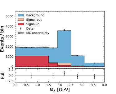
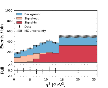
Figure 7: The post-fit distributions of the one-dimensional fits to $M_{X}$ and $q^{2}$ are shown, corresponding to the measured partial branching fractions for $E_{\ell}^{B}>1\,\text{GeV}$ with additional requirements of $M_{X}<1.7\,\text{GeV}$, and $M_{X}<1.7\,\text{GeV}$ and $q^{2}>8\,\text{GeV}^{2}$, respectively.

VIII Results

We report partial branching fractions for three phase-space regions from five fits to the reconstructed variables introduced in Section IV. All partial branching fractions correspond to a selection with $E_{\ell}^{B}>1\,\text{GeV}$, also reverting the effect of final state radiation photons, and possible additional phase-space restrictions. The resulting fit yields are listed in Table 5.

Table 5: The fitted signal yields in ($\widehat{\eta}_{\mathrm{sig}}$) and outside ($\widehat{\eta}_{\mathrm{sig-out}}$) the measured phase-space regions, the background yields ($\widehat{\eta}_{\mathrm{bkg}}$) and the product of tagging and selection efficiency are listed. The number of analyzed data events, $n_{\mathrm{data}}$, are also listed.

Phase-space region	Additional Selection	Fit variable(s)	$\widehat{\eta}_{\mathrm{sig}}$	$\widehat{\eta}_{\mathrm{sig-out}}$	$\widehat{\eta}_{\mathrm{bkg}}$	$n_{\mathrm{data}}$	$10^{3}\left(\epsilon_{\mathrm{tag}}\cdot\epsilon_{\mathrm{sel}}\right)$
$M_{X}<1.7$ GeV, $E_{\ell}^{B}>1$ GeV	-	$M_{X}$ fit	$1558\pm 69\pm 71$	$364\pm 51$	$6912\pm 138$	$8833\pm 94$	$0.26\pm 0.07$
$M_{X}<1.7$ GeV, $E_{\ell}^{B}>1$ GeV	$M_{X}<1.7\,\mathrm{GeV}$	$E_{\ell}^{B}$ fit	$1285\pm 68\pm 139$	$22\pm 3$	$1362\pm 155$	$2669\pm 52$	$0.21\pm 0.07$
$M_{X}<1.7$ GeV, $q^{2}>8$ GeV2, $E_{\ell}^{B}>1$ GeV	$M_{X}<1.7\,\mathrm{GeV}$	$q^{2}$ fit	$938\pm 99\pm 100$	$474\pm 57$	$1253\pm 192$	$2665\pm 52$	$0.14\pm 0.07$
$E_{\ell}^{B}>1$ GeV	$M_{X}<1.7\,\mathrm{GeV}$	$E_{\ell}^{B}$ fit	$1303\pm 69\pm 138$	-	$1366\pm 154$	$2669\pm 52$	$0.21\pm 0.19$
$E_{\ell}^{B}>1$ GeV		$M_{X}:q^{2}$ fit	$1801\pm 81\pm 123$	-	$7031\pm 164$	$8833\pm 94$	$0.31\pm 0.12$

VIII.1 Partial Branching Fraction Results

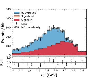
Figure 8: The post-fit distributions of the fit to $E_{\ell}^{B}$ with $M_{X}<1.7\,\text{GeV}$ is shown. The resulting yields were corrected to correspond to the partial branching fraction with $E_{\ell}^{B}>1\,\text{GeV}$ with and without an additional requirement of $M_{X}<1.7\,\text{GeV}$, respectively.

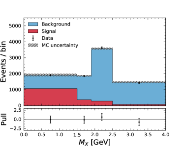
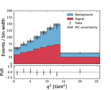
Figure 9: The post-fit projection of $M_{X}$ of the two-dimensional fit to $M_{X}:q^{2}$ on $M_{X}$ and the $q^{2}$ distribution in the range of $M_{X}\in[0,1.5]\,\mathrm{GeV}$ are shown. The resulting yields are corrected to correspond to a partial branching fraction with $E_{\ell}^{B}>1\,\text{GeV}$. The remaining $q^{2}$ distributions are given in Figure 22 (Appendix D).

For the partial branching fraction with $M_{X}<1.7\,\text{GeV}$ from the fit to $M_{X}$ we find

$$\Delta\mathcal{B}(B\to X_{u}\ell^{+}\,\nu_{\ell})=\left(1.09\pm 0.05\pm 0.08\right)\times 10^{-3}\,,$$ (27)

with the first and second error denoting the statistical and systematic uncertainty, respectively. The resulting post-fit distribution is shown in the top panel of Figure 7. With this selection about 56% of the available $B\to X_{u}\,\ell^{+}\,\nu_{\ell}$ phase space is probed. The partial branching fraction is in good agreement with the value obtained by fitting $E_{\ell}^{B}$ and corrected to the same phase space. The fit is shown in Figure 8 and we measure

$$\Delta\mathcal{B}(B\to X_{u}\ell^{+}\,\nu_{\ell})=\left(1.11\pm 0.06\pm 0.14\right)\times 10^{-3}\,,$$ (28)

with a larger systematic and statistical uncertainty than Eq. 27. To further probe the $B\to X_{u}\,\ell^{+}\,\nu_{\ell}$   enriched region, we carry out a measurement for $M_{X}<1.7\,\text{GeV}$ and $q^{2}>8\,\text{GeV}^{2}$ from a fit to the $q^{2}$ spectrum. This selection only probes about 31% of the available $B\to X_{u}\,\ell^{+}\,\nu_{\ell}$ phase space. We find

$$\Delta\mathcal{B}(B\to X_{u}\ell^{+}\,\nu_{\ell})=\left(0.67\pm 0.07\pm 0.10\right)\times 10^{-3}\,.$$ (29)

The corresponding post-fit distribution of $q^{2}$ is shown in the bottom panel of Figure 7. The most precise determinations of $B\to X_{u}\,\ell^{+}\,\nu_{\ell}$ are obtained from a two-dimensional fit, exploiting the full combined discriminatory power of $M_{X}$ and $q^{2}$. The resulting partial branching fraction probes about 86% of the available $B\to X_{u}\,\ell^{+}\,\nu_{\ell}$ phase space. We measure

$$\Delta\mathcal{B}(B\to X_{u}\ell^{+}\,\nu_{\ell})=\left(1.59\pm 0.07\pm 0.16\right)\times 10^{-3}\,.$$ (30)

The projection of the 2D fit onto $M_{X}$ and the $q^{2}$ distribution for the signal enriched region of $M_{X}<1.5\,\mathrm{GeV}$ are shown in Figure 9. The remaining $q^{2}$ distributions are given in Appendix D. The partial branching fraction is also in good agreement from the measurement obtained by fitting $E_{\ell}^{B}$, covering the same phase space (c.f. Figure 8):

$$\Delta\mathcal{B}(B\to X_{u}\ell^{+}\,\nu_{\ell})=\left(1.69\pm 0.09\pm 0.26\right)\times 10^{-3}\,.$$ (31)

The uncertainties are larger, but both results are compatible. The nuisance parameter pulls of all fits are provided in Appendix D. The result of Eq. 30 can be further compared with the most precise measurement to date of this region of Ref. Lees et al. (2017), where $\Delta\mathcal{B}(B\to X_{u}\ell\,\nu_{\ell})=\left(1.55\pm 0.12\right)\times 10^{-3}$, and shows good agreement. The measurement can also be compared to Ref. Lees et al. (2012) using a similar experimental approach. The measured partial branching fraction of $E_{\ell}^{B}>1\,\text{GeV}$ is $\Delta\mathcal{B}(B\to X_{u}\ell\,\nu_{\ell})=\left(1.82\pm 0.19\right)\times 10^{-3}$, which is compatible with Eq. 30 within 0.9 standard deviations. Belle previously reported in Ref. Urquijo et al. (2010) using also a similar approach for the same phase space a higher value of $\Delta\mathcal{B}(B\to X_{u}\ell\,\nu_{\ell})=\left(1.96\pm 0.19\right)\times 10^{-3}$. We cannot quantify the statistical overlap between both results, but by comparing the number of determined signal events one can estimate it to be below 55%. The dominant systematic uncertainties of Ref. Urquijo et al. (2010) were evaluated using different approaches, but fully correlating the dominant systematic uncertainties and assuming a statistical correlation of 55% we obtain a compatibility of 1.7 standard deviations. The main difference of this analysis with Ref. Urquijo et al. (2010) lies in the modeling of signal and background processes: since its publication our understanding improved and more precise measurements of branching fractions and form factors were made available. Further, for the $B\to X_{u}\,\ell^{+}\,\nu_{\ell}$ signal process in this paper a hybrid approach was adopted (see Section II and Appendix A), whereas Ref. Urquijo et al. (2010) used an alternative approach to model signal as a mix of inclusive and exclusive decay modes. Note that this work supersedes Ref. Urquijo et al. (2010).

VIII.2 $|V_{ub}|$ Determination

We determine $|V_{ub}|$ from the measured partial branching fractions using a range of theoretical rate predictions. In principle, the total $B\to X_{u}\,\ell^{+}\,\nu_{\ell}$ decay rate can be calculated using the same approach as $B\to X_{c}\,\ell^{+}\,\nu_{\ell}$ using the heavy quark expansion (HQE) in inverse powers of $m_{b}$. Unfortunately, the measurement requirements necessary to separate $B\to X_{u}\,\ell^{+}\,\nu_{\ell}$ from the dominant $B\to X_{c}\,\ell^{+}\,\nu_{\ell}$ background spoil the convergence of this approach. In the predictions for the partial rates corresponding to our measurements, perturbative and non-perturbative uncertainties are largely enhanced and as outlined in the introduction the predictions are sensitive to the shape function modeling.

The relationship between measured partial branching fractions, predictions of the rate (omitting CKM factors) $\Delta\Gamma(B\to X_{u}\,\ell^{+}\,\nu_{\ell})$, and $|V_{ub}|$ is

$$|V_{ub}|=\sqrt{\frac{\Delta\mathcal{B}(B\to X_{u}\,\ell^{+}\,\nu_{\ell})}{\tau_{B}\cdot\Delta\Gamma(B\to X_{u}\,\ell^{+}\,\nu_{\ell})}}\,.$$ (32)

with $\tau_{B}=\left(1.579\pm 0.004\right)\,\text{ps}$ denoting the average of the charged and neutral $\mathit{{B}{}_{\mspace{-3.0mu}\scriptstyle{}}^{\mspace{-1.0mu}\scriptstyle{}}}$ meson lifetime Zyla et al. (2020c). We use four predictions for the theoretical partial rates. All predictions use the same input values as Ref. Amhis et al. (2019) chooses for their world averages. The four predictions are:

• BLNP: The prediction of Bosch, Lange, Neubert, and Paz (short BLNP) of Ref. Lange et al. (2005a) provides a prediction at next-to-leading-order accuracy in terms of the strong coupling constant $\alpha_{s}$ and incorporates all known corrections. Predictions are interpolated between the shape-function dominated region (endpoint of the lepton spectrum, small hadronic mass) to the region of phase space, that can be described via the operator product expansion (OPE). As input we use $m_{b}^{\mathrm{SF}}=4.58\pm 0.03\,\text{GeV}$ and $\mu_{\pi}^{2\,\mathrm{SF}}=0.20{}^{+0.09}_{-0.10}\,\text{GeV}^{2}$.

• DGE: The Dressed Gluon Approximation (short DGE) from Andersen and Gardi Andersen and Gardi (2006); Gardi (2008) makes predictions by avoiding the direct use of shape functions, but produces predictions for hadronic observables using the on-shell $b$-quark mass. The calculation is carried out in the $\overline{\mathrm{MS}}$ scheme and we use $m_{b}(\overline{\mathrm{MS}})=4.19\pm 0.04\,\text{GeV}$.

• GGOU: The prediction from Gambino, Giordano, Ossola, and Uraltsev Gambino et al. (2007) (short GGOU) incorporates all known perturbative and non-perturbative effects up to the order $\mathcal{O}(\alpha_{s}^{2}\,\beta_{0})$ and $\mathcal{O}(1/m_{b}^{3})$, respectively. The shape function dependence is incorporated by parametrizing its effects in each structure function with a single light-cone function. The calculation is carried out in the kinetic scheme and we use as inputs $m_{b}^{\mathrm{kin}}=4.55\pm 0.02\,\,\text{GeV}$ and $\mu_{\pi}^{2\,\mathrm{kin}}=0.46\pm 0.08\,\text{GeV}^{2}$.

• ADFR: The calculation of Aglietti, Di Lodovico, Ferrera, and Ricciardi Aglietti et al. (2009, 2007) makes use of the ratio of $B\to X_{u}\,\ell^{+}\,\nu_{\ell}$ to $B\to X_{c}\,\ell^{+}\,\nu_{\ell}$ rates and soft-gluon resummation at next-to-next-to-leading-order and an effective QCD coupling approach. The calculation uses the $\overline{\mathrm{MS}}$ scheme and we use $m_{b}(\overline{\mathrm{MS}})=4.19\pm 0.04\,\text{GeV}$.

Table 6 lists the decay rates and their associated uncertainties for the probed regions of phase space, which we use to extract $|V_{ub}|$ from the measured partial branching fractions with Eq. 32.

Table 6: The theory rates $\Delta\Gamma(B\to X_{u}\,\ell^{+}\,\nu_{\ell})$ from various theory calculations are listed. The rates are given in units of $\text{ps}^{-1}$.

Phase-space region	BLNP Lange et al. (2005a)	DGE Andersen and Gardi (2006); Gardi (2008)	GGOU Gambino et al. (2007)	ADFR Aglietti et al. (2009, 2007)
$M_{X}<1.7\,\text{GeV}$	$45.2^{+5.4}_{-4.6}$	$42.3^{+5.8}_{-3.8}$	$43.7^{+3.9}_{-3.2}$	$52.3^{+5.4}_{-4.7}$
$M_{X}<1.7\,\text{GeV}$, $q^{2}>8\,\text{GeV}^{2}$	$23.4^{+3.4}_{-2.6}$	$24.3^{+2.6}_{-1.9}$	$23.3^{+3.2}_{-2.4}$	$31.1^{+3.0}_{-2.6}$
$E_{\ell}^{B}>1\,\mathrm{GeV}$	$61.5^{+6.4}_{-5.1}$	$58.2^{+3.6}_{-3.0}$	$58.5^{+2.7}_{-2.3}$	$61.5^{+5.8}_{-5.1}$

VIII.3 $|V_{ub}|$ Results

From the partial branching fractions with $E_{\ell}^{B}>1\,\text{GeV}$ and $M_{X}<1.7\,\text{GeV}$ determined from fitting $M_{X}$ we find

$$\left|V_{ub}\right|\,(\mathrm{BLNP}) =\left(3.90\pm 0.09\pm 0.15\pm 0.21\right)\times 10^{-3}\,,$$

$$\left|V_{ub}\right|\,(\mathrm{DGE}) =\left(4.08\pm 0.09\pm 0.16{}^{+0.20}_{-0.26}\right)\times 10^{-3}\,,$$

$$\left|V_{ub}\right|\,(\mathrm{GGOU}) =\left(3.97\pm 0.09{}^{+0.15}_{-0.16}{}^{+0.15}_{-0.16}\right)\times 10^{-3}\,,$$

$$\left|V_{ub}\right|\,(\mathrm{ADFR}) =\left(3.63\pm 0.08\pm 0.14\pm 0.17\right)\times 10^{-3}\,.$$ (33)

The uncertainties denote the statistical uncertainty, the systematic uncertainty and the theory error from the partial rate prediction. For the partial branching fraction with $E_{\ell}^{B}>1\,\text{GeV}$, $M_{X}<1.7\,\text{GeV}$, and $q^{2}>8\,\text{GeV}^{2}$ we find

$$\left|V_{ub}\right|\,(\mathrm{BLNP}) =\left(4.24{}^{+0.22}_{-0.23}{}^{+0.30}_{-0.32}{}^{+0.26}_{-0.28}\right)\times 10^{-3}\,,$$

$$\left|V_{ub}\right|\,(\mathrm{DGE}) =\left(4.16{}^{+0.21}_{-0.23}{}^{+0.30}_{-0.32}{}^{+0.18}_{-0.21}\right)\times 10^{-3}\,,$$

$$\left|V_{ub}\right|\,(\mathrm{GGOU}) =\left(4.25{}^{+0.22}_{-0.23}{}^{+0.30}_{-0.33}{}^{+0.24}_{-0.26}\right)\times 10^{-3}\,,$$

$$\left|V_{ub}\right|\,(\mathrm{ADFR}) =\left(3.68{}^{+0.19}_{-0.20}{}^{+0.26}_{-0.28}\pm 0.17\right)\times 10^{-3}\,.$$ (34)

Finally, the most inclusive determination with $E_{\ell}^{B}>1\,\text{GeV}$ from the two-dimensional fit of $M_{X}$ and $q^{2}$ results in

$$\left|V_{ub}\right|\,(\mathrm{BLNP}) =\left(4.05\pm 0.09{}^{+0.20}_{-0.21}{}^{+0.18}_{-0.20}\right)\times 10^{-3}\,,$$

$$\left|V_{ub}\right|\,(\mathrm{DGE}) =\left(4.16\pm 0.09{}^{+0.21}_{-0.22}{}^{+0.11}_{-0.12}\right)\times 10^{-3}\,,$$

$$\left|V_{ub}\right|\,(\mathrm{GGOU}) =\left(4.15\pm 0.09{}^{+0.21}_{-0.22}{}^{+0.08}_{-0.09}\right)\times 10^{-3}\,,$$

$$\left|V_{ub}\right|\,(\mathrm{ADFR}) =\left(4.05\pm 0.09{}^{+0.20}_{-0.21}\pm 0.18\right)\times 10^{-3}\,.$$ (35)

In order to quote a single value for $|V_{ub}|$ we adapt the procedure of Ref. Zyla et al. (2020b) and calculate a simple arithmetic average of the most precise determinations in Eq. 35 to obtain

$$\left|V_{ub}\right|=\left(4.10\pm 0.09\pm 0.22\pm 0.15\right)\times 10^{-3}\,.$$ (36)

This value is larger, but compatible with the exclusive measurement of $|V_{ub}|$ from $B\to\pi\,\ell^{+}\,\nu_{\ell}$ of $\left|V_{ub}\right|=\left(3.67\pm 0.09\pm 0.12\right)\times 10^{-3}$ within 1.3 standard deviations.

VIII.4 Stability Checks

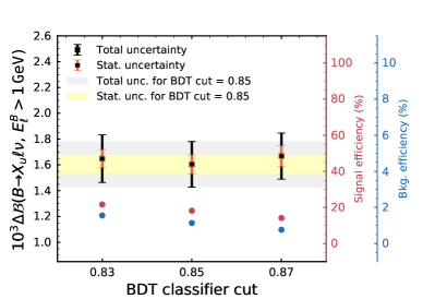
Figure 10: The stability of the determined partial branching fraction $\Delta\mathcal{B}(B\to X_{u}\ell\,\nu_{\ell})$ using the $M_{X}:q^{2}$ fit is studied as a function of the BDT selection requirement. The classifier output selection of $0.83$ and $0.87$ correspond to signal efficiencies after the pre-selection of 22% and 15%, respectively. These selections increase, or decrease the background from $B\to X_{c}\,\ell^{+}\,\nu_{\ell}$ and other processes by 37% and 33%, respectively. The grey and yellow bands show the total and statistical error, respectively, with the nominal BDT working point of 0.85.

To check the stability of the result we redetermine the partial branching fractions using two additional working points. We change the BDT selection to increase and decrease the amount of $B\to X_{c}\,\ell^{+}\,\nu_{\ell}$ and other backgrounds, and repeat the full analysis procedure. The resulting values of $\Delta\mathcal{B}(B\to X_{u}\ell\,\nu_{\ell})$ are determined using the two-dimensional fit of $M_{X}:q^{2}$ and are shown in Figure 10. The background contamination changes by $+37\%$ and $-33\%$, respectively. The small shifts in central value are well contained within the quoted systematic uncertainties. To further estimate the compatibility of the result we determine the full statistical and systematic correlations of the results and recover that the partial branching fraction with looser and tighter BDT selection are in agreement with the nominal result within 1.1 and 1.4 standard deviations, respectively.

VIII.5 $B\to X_{u}\,\ell^{+}\,\nu_{\ell}$ Charged Pion Multiplicity

Figure 11: The post-fit charged pion multiplicity is shown for events with $M_{X}<1.7$ GeV. The uncertainties on the MC stack include all systematic uncertainties.

The modeling the $B\to X_{u}\,\ell^{+}\,\nu_{\ell}$ signal composition is crucial to all presented measurements. One aspect difficult to assess is the $X_{u}$ fragmentation simulation: the charmless $X_{u}$ state can decay via many different channels producing a number of charged or neutral pions or kaons. In Section V we discussed how we assess the uncertainty on the number of $s\bar{s}$ quark pairs produced in the $X_{u}$ fragmentation. Due to the BDT removing such events to suppress the dominant $B\to X_{c}\,\ell^{+}\,\nu_{\ell}$ background, no signal-enriched region can be easily obtained. The accuracy of the fragmentation into the number of charged pions can be tested in the signal enriched region of $M_{X}<1.7\,\mathrm{GeV}$. Figure 11 compares the charged pion multiplicity between simulated signal and background processes and data. The signal and background predictions are scaled to their respective normalizations obtained from the two-dimensional fit in $M_{X}:q^{2}$. The uncertainty band shown on the MC includes the full systematic uncertainties discussed in Section V. The agreement overall lies within the assigned uncertainties, with the data having more events in the zero multiplicity bin and less in the two charged pion multiplicity bin. We use this distribution to correct our simulation to assign an additional uncertainty from the charged pion fragmentation. More details can be found in Section V and Appendix C.

VIII.6 Lepton Flavor Universality and Weak Annihilation Contributions

To test the lepton flavor universality in $B\to X_{u}\,\ell^{+}\,\nu_{\ell}$ we also carry out fits to determine the partial branching fraction for electron and muon final states. For this we categorzie the selected events accordingly and carry out a fit to the $M_{X}:q^{2}$ distributions using the same granularity as the fit described in Section VIII.1. We carry out a simultaneous analysis of both samples, such that shared NPs for the modeling of the signal or background components can be correctly correlated afterwards. The resulting yields are corrected to a partial branching fraction with $E_{\ell}^{B}>1\,\text{GeV}$ and we obtain

$$\Delta\mathcal{B}(B\to X_{u}e^{+}\,\nu_{e})=\left(1.57\pm 0.10\pm 0.16\right)\times 10^{-3}\,,$$ (37)

$$\Delta\mathcal{B}(B\to X_{u}\mu^{+}\,\nu_{\mu})=\left(1.62\pm 0.10\pm 0.18\right)\times 10^{-3}\,,$$ (38)

with a total correlation of $\rho=0.53$. The ratio of the electron to the muon final state is

$$R_{e\mu}=\frac{\Delta\mathcal{B}(B\to X_{u}e^{+}\,\nu_{e})}{\Delta\mathcal{B}(B\to X_{u}\mu^{+}\,\nu_{\mu})}=0.97\pm 0.09\pm 0.04\,,$$ (39)

with the first error denoting the statistical uncertainty and the second the systematic uncertainty. We observe no significant deviation from lepton flavor universality. More details on the fit can be found in Appendix E.

Isospin breaking effects can be studied by separately measuring the partial branching fraction for charged and neutral $B$ meson final states. We determine the ratio

$$R_{\mathrm{iso}}=\frac{\tau_{B^{0}}}{\tau_{B^{+}}}\times\frac{\Delta\mathcal{B}(B^{+}\to X_{u}\ell^{+}\,\nu_{\ell})}{\Delta\mathcal{B}(B^{0}\to X_{u}\ell^{+}\,\nu_{\ell})}\,,$$ (40)

by using the information from the composition of the fully reconstructed tag-side $B$-meson decays to separate charged and neutral $B$ candidates. The partial branching fraction is then determined by a simultaneous fit of both samples in $M_{X}:q^{2}$ to correctly correlate common systematic uncertainties. To account for the small contamination of wrongly assigned $B$ tag flavors, we use the wrong-tag fractions from our simulation. The measured number of signal events in the reconstructed neutral and charged $B$ candidate categories (denoted in the following as $N_{\mathrm{reco}}^{0}$ and $N_{\mathrm{reco}}^{+}$) are related to the number of neutral and charged $B$ mesons ($N_{\mathrm{true}}^{0}$ and $N_{\mathrm{true}}^{+}$) via

$$N_{\mathrm{reco}}^{0}=\mathcal{P}_{B^{0}_{\mathrm{true}}\to B^{0}_{\mathrm{reco}}}\,N_{\mathrm{true}}^{0}+\mathcal{P}_{B^{+}_{\mathrm{true}}\to B^{0}_{\mathrm{reco}}}\,N_{\mathrm{true}}^{+}\,,$$ (41)

$$N_{\mathrm{reco}}^{+}=\mathcal{P}_{B^{0}_{\mathrm{true}}\to B^{+}_{\mathrm{reco}}}\,N_{\mathrm{true}}^{0}+\mathcal{P}_{B^{+}_{\mathrm{true}}\to B^{+}_{\mathrm{reco}}}\,N_{\mathrm{true}}^{+}\,.$$ (42)

Here e.g. $\mathcal{P}_{B^{0}_{\mathrm{true}}\to B^{+}_{\mathrm{reco}}}$ denotes the probability to identify in the reconstruction of the tag-side $B$-meson a true $B^{0}$ as a $B^{+}$ candidate. In the simulation we find

$$\mathcal{P}_{B^{0}_{\mathrm{true}}\to B^{0}_{\mathrm{reco}}}=0.985\,\quad\mathcal{P}_{B^{0}_{\mathrm{true}}\to B^{+}_{\mathrm{reco}}}=0.015\,,$$ (43)

$$\mathcal{P}_{B^{+}_{\mathrm{true}}\to B^{+}_{\mathrm{reco}}}=0.977\,\quad\mathcal{P}_{B^{+}_{\mathrm{true}}\to B^{0}_{\mathrm{reco}}}=0.023\,.$$ (44)

Using this procedure we determine for the individual partial branching fractions with $E_{\ell}^{B}>1\,\text{GeV}$

$$\Delta\mathcal{B}(B^{+}\to X_{u}\ell^{+}\,\nu_{\ell})=\left(1.65\pm 0.10\pm 0.18\right)\times 10^{-3}\,,$$ (45)

$$\Delta\mathcal{B}(B^{0}\to X_{u}\ell^{+}\,\nu_{\ell})=\left(1.51\pm 0.10\pm 0.16\right)\times 10^{-3}\,,$$ (46)

with a total correlation of $\rho=0.50$ and for the ratio Eq. 40

$$R_{\mathrm{iso}}=1.01\pm 0.09\pm 0.06\,,$$ (47)

compatible with the expectation of equal semileptonic rates for both isospin states. Isospin breaking effects would for instance arise from weak annihilation contributions, which only can contribute to charged $B$ meson final states. Using Eq. 47 the relative contribution from weak annihilation processes to the total semileptonic $B\to X_{u}\ell^{+}\,\nu_{\ell}$ rate can be constrained via

$$\frac{\Gamma_{\mathrm{wa}}}{\Gamma(B\to X_{u}\ell^{+}\,\nu_{\ell})}=\frac{f_{u}}{f_{\mathrm{wa}}}\times\left(R_{\mathrm{iso}}-1\right)\,.$$ (48)

Here $f_{u}$ is a factor that corrects the measured partial branching fraction to the full inclusive phase space. We estimate it using the DFN model De Fazio and Neubert (1999) (cf. Section II for details) and find $f_{u}=0.86$. We further assume that $f_{\mathrm{wa}}=1$, as such processes would produce a high momentum lepton. We recover

$$\frac{\Gamma_{\mathrm{wa}}}{\Gamma(B\to X_{u}\ell^{+}\,\nu_{\ell})}=0.01\pm 0.09\,,$$ (49)

which translates into a limit of $[-0.14,0.17]$ at 90% CL. This result is more stringent than the limit of Ref. Lees et al. (2012), but weaker than the result of Ref. Rosner et al. (2006), that directly used the shape of the $q^{2}$ distribution to constrain weak annihilation processes. Our result is also weaker than the estimates of Refs. Gambino and Kamenik (2010); Ligeti et al. (2010); Voloshin (2001); Bigi and Uraltsev (1994) that constrain weak annihilation contributions to be of the order 2-3%.

IX Summary and Conclusions

We report measurements of partial branching fractions with different requirements on the properties of the hadronic system of the $B\to X_{u}\,\ell^{+}\,\nu_{\ell}$ decay and with a lepton energy of $E_{\ell}^{B}>1\,\text{GeV}$ in the $\mathit{{B}{}_{\mspace{-3.0mu}\scriptstyle{}}^{\mspace{-1.0mu}\scriptstyle{}}}$ rest-frame, covering 31-86% of the available phase space. The sizeable background from semileptonic $B\to X_{c}\,\ell^{+}\,\nu_{\ell}$ decays is suppressed using multivariate methods in the form of a BDT. This approach allows us to reduce such backgrounds to an acceptable level, whilst retaining a high signal efficiency. Signal yields are obtained using a binned likelihood fit in either the reconstructed hadronic mass $M_{X}$, the four-momentum-transfer squared $q^{2}$, or the lepton energy $E_{\ell}^{B}$. The most precise result is obtained from a two-dimensional fit of $M_{X}$ and $q^{2}$. Translated to a partial branching fraction for $E_{\ell}^{B}>1\,\text{GeV}$ we obtain

$$\Delta\mathcal{B}(B\to X_{u}\ell^{+}\,\nu_{\ell})=\left(1.59\pm 0.07\pm 0.16\right)\times 10^{-3}\,,$$ (50)

with the errors denoting statistical and systematic uncertainties. The partial branching fraction is compatible with the value obtained by a fit of the lepton energy spectrum $E_{\ell}^{B}$ and with the most precise determination of Ref. Lees et al. (2017). In addition, it is stable under variations of the background suppression BDT. From this partial branching fraction we obtain a value of

$$\left|V_{ub}\right|=\left(4.10\pm 0.09\pm 0.22\pm 0.15\right)\times 10^{-3}$$ (51)

from an average over four theoretical calculations. This value is higher than, but compatible with, the value of $|V_{ub}|$ from exclusive determinations by 1.3 standard deviations. The compatibility with the value expected from CKM unitarity from a fit of Ref. Charles et al. (2005) of $|V_{ub}|=\left(3.62{}^{+0.11}_{-0.08}\right)\times 10^{-3}$ is 1.6 standard deviations. Figure 12 summarizes the situation. The result presented here supersedes Ref. Urquijo et al. (2010): this paper uses a more efficient tagging algorithm, incorporates improvements of the $B\to X_{u}\,\ell^{+}\,\nu_{\ell}$ signal and $B\to X_{c}\,\ell^{+}\,\nu_{\ell}$ background descriptions, and analyzes the full Belle data set of 711 fb^-1. The measurement of kinematic differential shapes of $M_{X}$, $q^{2}$, and other properties are left for future work. These results will be crucial for future direct measurements with Belle II that will attempt to use data-driven methods to directly constrain the shape function using $B\to X_{u}\,\ell^{+}\,\nu_{\ell}$ information.

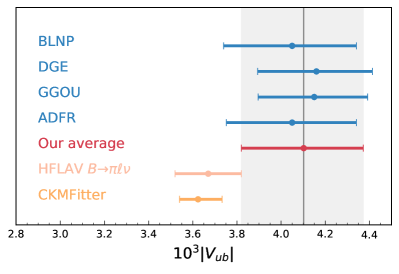
Figure 12: The obtained values of $|V_{ub}|$ from the four calculations and the arithmetic average is compared to the determination from exclusive $B\to\pi\,\ell^{+}\,\nu_{\ell}$ and the expectation from CKM unitarity Charles et al. (2005) without the direct constraints from semileptonic and leptonic decays.

A. $B\to X_{u}\,\ell^{+}\,\nu_{\ell}$ Hybrid MC Details

Figure 13 shows the generator level hybrid $B\to X_{u}\,\ell^{+}\,\nu_{\ell}$ signal sample for $E_{\ell}^{B}$, $M_{X}$, and $q^{2}$ described in Section II.

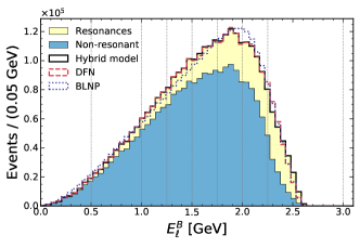
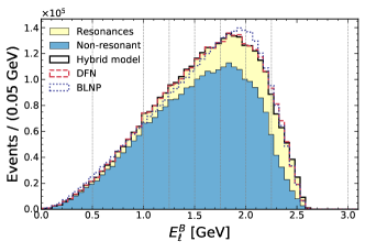
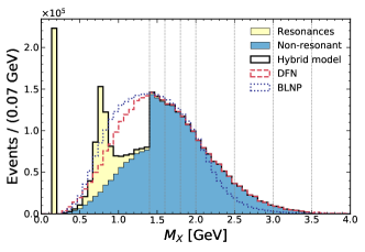
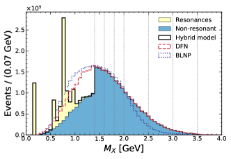
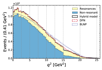
Figure 13: The generator level $B\to X_{u}\,\ell^{+}\,\nu_{\ell}$ distributions $E_{\ell}^{B}$, $M_{X}$, and $q^{2}$ for neutral (left) and charged (right) $B$ mesons are shown. The black histogram shows the merged hybrid model, composed of resonant and non-resonant contributions. For more details on the used models and how the hybrid $B\to X_{u}\,\ell^{+}\,\nu_{\ell}$ signal sample is constructed, see Section II.

B. Input variables of $B\to X_{c}\ell\bar{\nu}_{\ell}$ suppression BDT

The shapes of the variables used in the $B\to X_{c}\,\ell^{+}\,\nu_{\ell}$ background suppression BDT are shown in Figures 14 and 17. The most discriminating variables are $M_{\mathrm{miss}}^{2}$, the $B_{\mathrm{sig}}$ vertex fit probability, and $M_{\mathrm{miss},D^{*}}^{2}$. Figures 15, 16 and 18 show the agreement between recorded and simulated events, taking into account the full uncertainties detailed in Section V. More details about the BDT can be found in Section III.3.

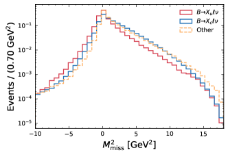
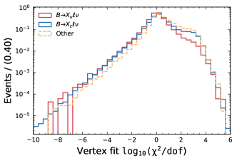
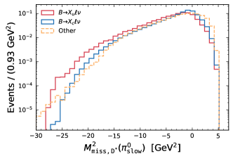
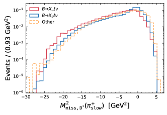
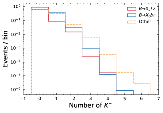
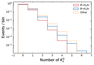
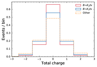
Figure 14: The shape of the input variables for the $B\to X_{c}\,\ell^{+}\,\nu_{\ell}$ background suppression BDT are shown. For details and definitions see Section III.3.

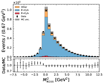
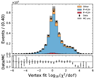
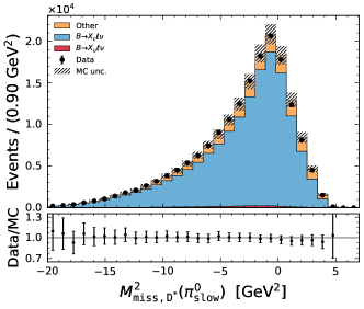
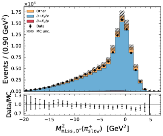
Figure 15: The input variables for the $B\to X_{c}\,\ell^{+}\,\nu_{\ell}$ background suppression BDT for recorded and simulated events are shown. The uncertainty on the simulated events incorporate the full systematic uncertainties detailed in Section V.

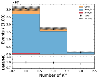
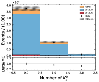
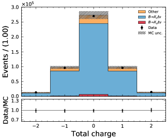
Figure 16: The input variables for the $B\to X_{c}\,\ell^{+}\,\nu_{\ell}$ background suppression BDT for recorded and simulated events are shown. The uncertainty on the simulated events incorporate the full systematic uncertainties detailed in Section V.

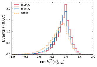
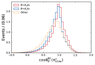
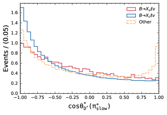
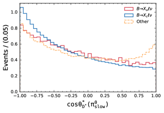
Figure 17: The shape of the input variables for the $B\to X_{c}\,\ell^{+}\,\nu_{\ell}$ background suppression BDT are shown. For details and definitions see Section III.3.

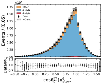
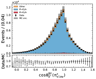
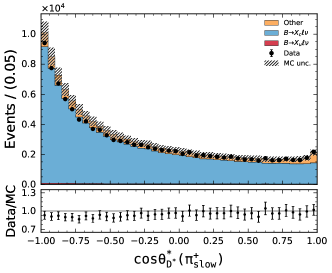
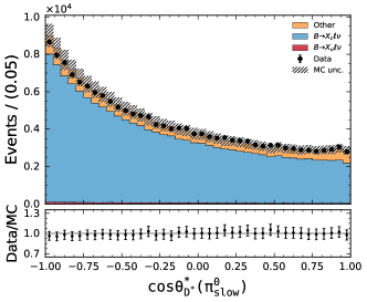
Figure 18: The input variables for the $B\to X_{c}\,\ell^{+}\,\nu_{\ell}$ background suppression BDT for recorded and simulated events are shown. The uncertainty on the simulated events incorporate the full systematic uncertainties detailed in Section V.

C. $B\to X_{u}\,\ell^{+}\,\nu_{\ell}$ Charged Pion Fragmentation modeling

Figure 19 compares the charged pion multiplicity at different stages in the selection. This variable is not used in the signal extraction, but its modeling is tested to make sure that the $B\to X_{u}\,\ell^{+}\,\nu_{\ell}$ fragmentation probabilities cannot bias the final result. The agreement in the signal enriched region with $M_{X}<1.7$ GeV after the BDT selection is fair, but shows some deviations. We correct the generator level charged pion multiplicity to match the $n_{\pi^{\pm}}$ observed in this selection by assigning the non-resonant $B\to X_{u}\,\ell^{+}\,\nu_{\ell}$ events a correction weight as a function of the true charged pion multiplicity. After this procedure the agreement is perfect and we use the difference in the reconstruction efficiency as an uncertainty on the pion fragmentation on the partial branching fractions and $|V_{ub}|$ (cf. Section V).

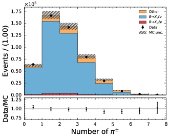
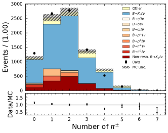
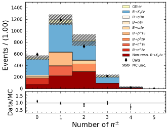
Figure 19: The charged pion multiplicity ($n_{\pi^{\pm}}$) are compared between data and the simulation: (top left) for all events prior the BDT selection; (top right) for all events after the BDT selection; (bottom left): for the signal enriched region of $M_{X}<1.7$ GeV; (bottom right) for the same region but after rescaling the non-resonant contributions such that the $n_{\pi^{\pm}}$ fragmentation probability to match the one observed in data.

D. Nuisance Parameter Pulls and Additional Fit Plots

Figures 20 and 21 show the nuisance parameter pulls for each fit category $k$ and bin $i$ defined as

$$\left(\widehat{\theta}_{ik}-\theta_{ik}\right)/\sqrt{\Sigma_{k,ii}}\,,$$ (52)

of the partial branching fraction fits, with $\widehat{\theta}$ ($\theta$) corresponding to the post-fit (pre-fit) value of the nuisance parameter. Note that uncertainties of each pull shows the post-fit error

$$\sqrt{\widehat{\Sigma}_{k,ii}}$$ (53)

normalized to the pre-fit constraint

$$\sqrt{\Sigma_{k,ii}}\,.$$ (54)

Figure 22 shows the post-fit $q^{2}$ distributions of the two-dimensional fit to $M_{X}:q^{2}$ on $M_{X}$.

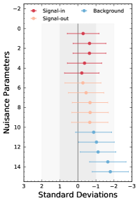
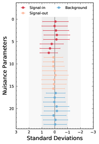
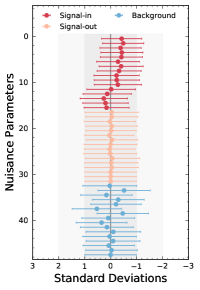
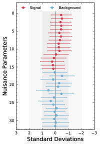
Figure 20: The nuisance parameter pulls on the 1D fits of $M_{X}$, $q^{2}$, and $E_{\ell}^{B}$ with and without $M_{X}<1.7$ GeV events separated out, are shown from left to right.

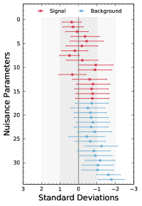
Figure 21: The nuisance parameter pulls on the 2D fit of $M_{X}:q^{2}$ is shown.

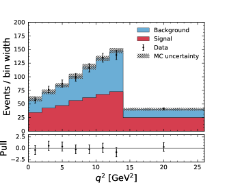
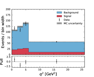
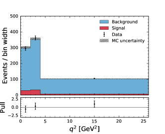
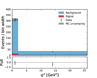
Figure 22: The post-fit $q^{2}$ distributions of the two-dimensional fit to $M_{X}:q^{2}$ on $M_{X}$ are shown. The panels correspond to: $M_{X}\in[0,1.5]\,\mathrm{GeV}$ (top left), $M_{X}\in[1.5,1.9]\,\mathrm{GeV}$ (top right), $M_{X}\in[1.9,2.4]\,\mathrm{GeV}$ (bottom left) and $M_{X}\in[2.4,4]\,\mathrm{GeV}$ (bottom right). The resulting yields are corrected to correspond to a partial branching fraction with $E_{\ell}^{B}>1\,\text{GeV}$.

E. Additional Fit Details to the Lepton Flavor Universality and Weak Annihilation Tests

The fitted yields of the two-dimensional fit to $M_{X}:q^{2}$ separated in electron and muon candidates, as well as in charged or neutral $B$ mesons are listed in Table 7.

Table 7: The fitted yields separated in electron and muon candidates, as well as in charged or neutral $B$ mesons.

Decay mode	$\widehat{\eta}_{\tt{sig}}$	$\widehat{\eta}_{\tt{bkg}}$	$10^{3}\left(\epsilon_{\tt{tag}}\cdot\epsilon_{\tt{sel}}\right)$	$10^{3}\Delta\mathcal{B}$
$B^{+}\to X_{u}\ell^{+}\nu$	$914\pm 56\pm 64$	$3667\pm 77\pm 63$	$0.30\pm 0.13$	$1.65\pm 0.10\pm 0.18$
$B^{0}\to X_{u}\ell^{+}\nu$	$879\pm 58\pm 65$	$3373\pm 76\pm 64$	$0.33\pm 0.11$	$1.51\pm 0.10\pm 0.16$
$B\to X_{u}e^{+}\nu$	$870\pm 56\pm 59$	$3311\pm 75\pm 60$	$0.31\pm 0.12$	$1.57\pm 0.10\pm 0.16$
$B\to X_{u}\mu^{+}\nu$	$936\pm 58\pm 71$	$3716\pm 78\pm 71$	$0.32\pm 0.13$	$1.62\pm 0.10\pm 0.18$

F. BDT Efficiencies

Figure 23 shows the efficiency of the BDT selection as a function of the reconstructed variables $q^{2}$, $M_{X}$, and the lepton energy $E_{\ell}^{B}$ for simulated $B\to X_{u}\,\ell^{+}\,\nu_{\ell}$ events. Although we avoided using these variables in the boosted decision tree, a residual dependence on the kinematic variables is seen. For instance the efficiency increases with an increase in $E_{\ell}^{B}$ and a decrease with respect to high $q^{2}$. The efficiency on the hadronic mass $M_{X}$ is relatively flat. This efficiency dependence is linked to the used variables in the BDT. Although we carefully avoided kinematic variables that would allow the BDT to learn these kinematic properties, there are indirect connections: e.g. high $E_{\ell}^{B}$ final states have a lower multiplicity as they are dominated by $B\to\pi\ell\bar{\nu}_{\ell}$ decays. Further, their corresponding hadronic system carries little momentum and on average such decays retain a better resolution in discriminating variables of the background suppression BDT. A concrete example is $M_{\mathrm{miss}}^{2}$ (cf. Figure 15): high multiplicity $B\to X_{u}\,\ell^{+}\,\nu_{\ell}$ decays will retain a larger tail in this variable and will be selected with a lower efficiency by the BDT.

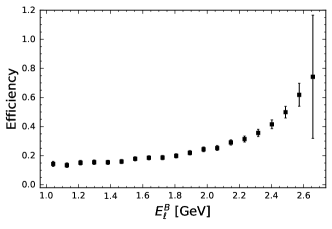
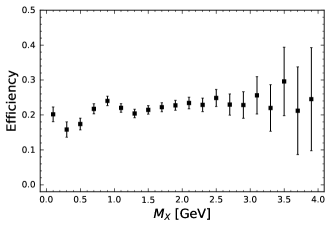
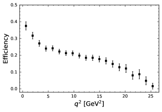
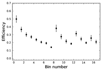
Figure 23: The $B\to X_{u}\,\ell^{+}\,\nu_{\ell}$ efficiency after the BDT selection is shown as a function of the reconstructed kinematic variables ($E_{\ell}^{B}$, $M_{X}$, $q^{2}$) used in the signal extraction. The bottom right plot shows the efficiencies in the bins of $M_{X}:q^{2}$ and the binning can be found in the text. The uncertainties are statistical only.