Hamiltonian reconstruction as metric for variational studies

Abstract

Variational approaches are among the most powerful modern techniques to approximately solve quantum many-body problems. These encompass both variational states based on tensor or neural networks, and parameterized quantum circuits in variational quantum eigensolvers. However, self-consistent evaluation of the quality of variational wavefunctions is a notoriously hard task. Using a recently developed Hamiltonian reconstruction method, we propose a multi-faceted approach to evaluating the quality of neural-network based wavefunctions. Specifically, we consider convolutional neural network (CNN) and restricted Boltzmann machine (RBM) states trained on a square lattice spin-1/2 $J_{1}$-$J_{2}$ Heisenberg model. We find that the reconstructed Hamiltonians are typically less frustrated, and have easy-axis anisotropy near the high frustration point. Furthermore, the reconstructed Hamiltonians suppress quantum fluctuations in the large $J_{2}$ limit. Our results highlight the critical importance of the wavefunction’s symmetry. Moreover, the multi-faceted insight from the Hamiltonian reconstruction reveals that a variational wave function can fail to capture the true ground state through suppression of quantum fluctuations.

Introduction – The Hamiltonian is the defining object that governs the dynamics of a physical system. For a quantum mechanical system, it defines the Schrödinger equation to be solved to obtain the energy spectrum and the wavefunction. However, the approach of “exact diagonalization” is constrained to small system sizes due to the exponential growth of the Hilbert space upon increasing the system size. An alternative to exact diagonalization is the Quantum Monte Carlo techniques using a stochastic approach to model the probability distribution associated with the thermal density matrix associated with a given Hamiltonian. These approaches, however, suffer from the sign-problem Troyer and Wiese (2005), which limits their applicability to a restricted class of Hamiltonians, or to high temperature properties only. These challenges motivated variational wavefunction approaches to start from many-body wave functions that are parameterized within a given functional form. In variational approaches, the Hamiltonian is referenced for optimizing the wavefunction within the chosen functional form (see the blue arrow in Figure 1). Since the resulting best wavefunction is constrained to lie within limited variational spaces such as tensor network states Verstraete et al. (2008), neural network states Carleo and Troyer (2017); Choo et al. (2019), and parametrized quantum circuits Peruzzo et al. (2014); McClean et al. (2016) (see Figure 1), significant effort has been put into having sufficiently general variational classes that can capture the actual ground state. However, assessing how close a given variational parameterization is to the target ground state is, in general, a hard task.

At present, the standard metrics for assessing the quality of a wavefunction that cut across different variational forms are the energy and the energy variance. Reliance on these measurements, however, leaves the comparison between constructions a case-by-case trial exercise. Much needed are alternative metrics to assess the quality of a given variational state. Interestingly, recent works have proposed methods to reconstruct Hamiltonians from measurements of correlators Qi and Ranard (2019); Chertkov and Clark (2018); Bairey et al. (2019); Valenti et al. (2019) or single operator measurements Pakrouski (2020) (see the red arrow in Figure 1). These reconstruction processes have been tested on Hamiltonians with known exact solutions, but their applicability to challenging open problems has yet to be demonstrated.

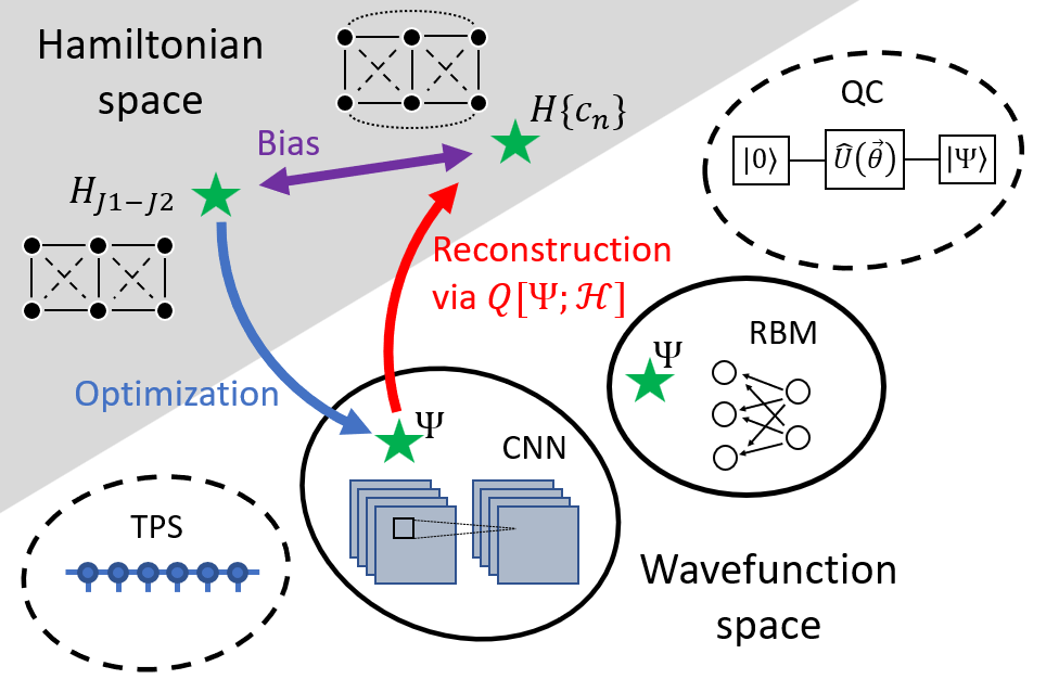
Figure 1: In a typical variational algorithm, a wavefunction is obtained through variational optimization within a given variational form such as CNN, RBM, tensor product state (TPS), or a parametrized quantum circuit (QC). In this work, we study CNN and RBM quantum states, marked with green stars. A blue arrow is shown to represent variational optimization of the CNN construction as an example. The Hamiltonian reconstruction works in the opposite direction to map a variational wavefunction to a Hamiltonian $H[\{c_{n}\}]$ (red arrow). The bias between the original Hamiltonian and the reconstructed Hamiltonian (purple arrow) provides insight into the nature of the variational wavefunction.

In this Letter, we employ Hamiltonian reconstruction to investigate how frustration affects the distance between reconstructed and target Hamiltonians for neural-network wavefunctions. We optimize convolutional neural network (CNN) and restricted Boltzmann machine (RBM) wavefunctions to approximate the ground state of the spin-1/2 $J_{1}$-$J_{2}$ Heisenberg model on a square lattice Choo et al. (2019), a poster-child frustrated spin model that suffers from the sign problem. On this model, deep neural network-based wavefunctions have so far obtained highly accurate results for the $J_{1}$-$J_{2}$ model away from the high frustration point, showing the potential of neural-network based variational constructions. However, the same neural network states showed limitations near $J_{2}/J_{1}=0.5$, which is the point of high frustration Choo et al. (2019). To probe features of these wavefunctions, we construct subspaces of Hamiltonians that accommodate different “deformations” of the target Hamiltonian. For each subspace, we use the reconstruction method to retrieve the Hamiltonian that best fits the trained wavefunction. We then discuss insights from the Hamiltonian reconstruction.

Hamiltonian Reconstruction – Let us review the Hamiltonian reconstruction procedure following Refs. Qi and Ranard (2019); Chertkov and Clark (2018). The procedure starts with the wavefunction of interest $\Psi$, which would be energy-optimized within a given variational form. We then define the Hamiltonian subspace, to be searched within, by a spanning set of operators $\mathcal{O}\equiv\{O_{i}\}$. Any Hamiltonian that is an element of this subspace, i.e., $H\in\mathcal{H}$, can be expressed in the form

$$H[\{c_{n}\}]=\sum_{n}^{N}c_{n}O_{n},$$ (1)

where $c_{n}$’s are real-valued parameters. The aim of the reconstruction procedure is to find the $N$-dimensional vector $\{c_{n}\}$ such that the wavefunction of interest $|\Psi\rangle$ is an approximate eigenstate of the corresponding Hamiltonian $H[\{c_{n}\}]$. For this, we construct the quantum covariance matrix $Q$ associated with the wavefunction and the Hamiltonian subspace

$$Q[\Psi;\mathcal{H}]_{nm}=\frac{1}{2}\left(\langle O_{n}O_{m}\rangle+\langle O_{m}O_{n}\rangle\right)-\langle O_{n}\rangle\langle O_{m}\rangle,$$ (2)

which is an $N\crossproduct N$ positive semi-definite matrix where expectation values are evaluated with respect to the wavefunction $|\Psi\rangle$ (also see Figure 1). The computational cost of evaluating $Q$ is quadratic in the number of operators to be considered (but note that the number of terms in operators also tends to grow linearly with system size).

The subset of Hamiltonians $\mathcal{H}[\mathcal{O}]$ that correspond to eigenvectors of $Q[\Psi;\mathcal{H}]$ with the smallest eigenvalues would all accept $|\Psi\rangle$ as an approximate eigenstate. To see this, note that the variance of the Hamiltonian $H[\{c_{n}\}]$ in the state $\ket{\Psi}$ is given by

$$\begin{split}\langle(\Delta H[\{c_{n}\}])^{2}\ &=\langle H[\{c_{n}\}]^{2}\rangle-\langle H[\{c_{n}\}]\rangle^{2}\\ &=\sum_{nm}c_{n}c_{m}\left(\langle O_{n}O_{m}\rangle-\langle O_{n}\rangle\langle O_{m}\rangle\right)\\ &=\vec{c}^{~{}T}Q[\Psi;\mathcal{H}]\vec{c}.\end{split}$$ (3)

By diagonalizing $Q[\Psi;\mathcal{H}]$, the Hamiltonians $H[\{c_{n}\}]$ which have the lowest variance under $\ket{\Psi}$ can be found, and the associated eigenvalues will be the variances in energy of those Hamiltonians. If $|\Psi\rangle$ is an exact ground state of the exact parent Hamiltonian $H^{*}$, and $H^{*}$ is within the Hamiltonian search space $\mathcal{H}[\mathcal{O}]$, then $H^{*}$ will lie in the nullspace of $Q[\Psi;\mathcal{H}]$.

The expectation values of many-body operators in Eq. (2) need to be evaluated by performing high-dimensional integrals. Typically, these high-dimensional integrals can be approximated via Monte Carlo (MC) sampling, but we found that the Hamiltonian reconstruction is highly sensitive to noise in the correlation functions (see Supplemental Material II.C). This sensitivity restricts the procedure to systems in which the correlation functions can be evaluated sufficiently accurately; indeed, previous applications of Hamiltonian reconstruction Chertkov and Clark (2018); Dupont and Laflorencie (2019) are limited to well-understood states in which correlation functions can be evaluated easily. In our case, this restricted our study to small system sizes in which the correlation functions could be evaluated explicitly.

The antiferromagnetic $J_{1}$-$J_{2}$ model for spin 1/2 on a two-dimensional square lattice Dagotto and Moreo (1989); Schulz and Ziman (1992) is defined by the following Hamiltonian

$$H_{J_{1}J_{2}}\equiv J_{1}\sum_{\langle ij\rangle}\vec{S}_{i}\cdot\vec{S}_{j}+J_{2}\sum_{\llangle ij\rrangle}\vec{S}_{i}\cdot\vec{S}_{j},$$ (4)

where $\langle ij\rangle$ and $\llangle ij\rrangle$ denote nearest and next-nearest neighbours respectively. We set $J_{1}=1$ and consider only antiferromagnetic interactions $J_{2}\geq 0$. The exact ground states of the Hamiltonian in the two limits of $J_{2}\ll J_{1}$ and $J_{2}\gg J_{1}$ are well understood, since geometric frustration is absent in both limits: the ground state is a Néel antiferromagnet for $J_{2}\ll J_{1}$ and a striped antiferromagnet for $J_{2}\gg J_{1}$. However, the nature of the ground state in the vicinity of the maximally frustrated point of $J_{2}/J_{1}=0.5$ is the subject of much debate Hu et al. (2013); Gong et al. (2014); Jiang et al. (2012); Sachdev and Bhatt (1990); Mambrini et al. (2006); Yu and Kao (2012); Wang and Sandvik (2018); Ferrari and Becca (2020); Nomura and Imada (2020a).

Hamiltonian space and wavefunction space – We consider three Hamiltonian subspaces that allow the reconstructed Hamiltonian to deviate from the target Hamiltonian Eq. (4) in physically meaningful ways. We chose the three two-operator parametrizations

$$\begin{split}H[\delta J_{2}]&=H_{J_{1}J_{2}}+\delta J_{2}\sum_{\llangle i,j\rrangle}\vec{S}_{i}\cdot\vec{S}_{j}\\ H[J_{3}]&=H_{J_{1}J_{2}}+J_{3}\sum_{\left<i,j\right>_{3}}\vec{S}_{i}\cdot\vec{S}_{j}\\ H[\alpha]&=H_{J_{1}J_{2}}+\alpha\left(\sum_{\left<i,j\right>}S^{z}_{i}S^{z}_{j}+\frac{J_{2}}{J_{1}}\sum_{\llangle i,j\rrangle}S^{z}_{i}S^{z}_{j}\right),\\ \end{split}$$ (5)

where $\delta J_{2}$ measures the degree of frustration, $J_{3}$ measures the strength of a longer range interaction, and $\alpha$ measures the easy-axis anisotropy. Above, the coefficients of the original $J_{1}$-$J_{2}$ Hamiltonian have been normalized to 1. In Supplemental Material – II.A, we show that reconstructions into these spaces, from an exact solution of the Heisenberg model, simply yield the original Heisenberg model. In Supplemental Material – II.B, we present how reconstructions into higher-dimensional spaces are more challenging to interpret, motivating our choice of study of two-dimensional Hamiltonian spaces.

Seeking further understanding of the challenges underlying the maximally frustrated point, we focus on neural network based wavefunctions that outperformed (i.e., had lower energy than) leading variational constructions, away from the high frustration point Choo et al. (2019). Neural networks can be universal approximators of complex functions Cybenko (1989); Bishop (1995) and thus have the potential to allow more efficient exploration of the wavefunction space compared to traditional constructions Deng et al. (2017). The initial proposal of using restricted Boltzmann machines (RBM) to represent many-body wavefunctions Carleo and Troyer (2017) generated much excitement in the community and extensive investigations of RBM-based wavefunctions and their variants Nomura et al. (2017); Carleo et al. (2018); Chen et al. (2018); Glasser et al. (2018); Saito and Kato (2018); Choo et al. (2018); Kochkov and Clark (2018); Luo and Clark (2019); Pastori et al. (2019); Sharir et al. (2020); Nomura and Imada (2020b); Gao and Duan (2017). More recently, Levine et al. (2019) showed that the more expressive convolutional neural network (CNN) architecture can encode volume-law entangled states more efficiently. Indeed, CNN wavefunctions improved energy compared to state-of-the-art methods for the $J_{1}$-$J_{2}$ model, but only in the parameter regime away from the classical frustration point of $J_{2}/J_{1}=0.5$ Choo et al. (2019).

In this work, we examine CNN and RBM many-body wavefunctions which were trained to to have high overlap with the ground state of the model in question, the spin-1/2 Heisenberg $J_{1}$-$J_{2}$ model on a $4\times 4$ square lattice with periodic boundary conditions (see Supplemental Material I). Both the CNN and RBM architectures preserve the translational invariance of the system, and the wavefunctions were further symmetrized to respect time reversal and point group symmetries (see Supplemental Material – I.C). We trained wavefunctions for values of $J_{2}$ ranging between 0 and 2. The optimization of the wavefunctions was done using the NetKet package Carleo et al. (2019).

Results – The conventional measure for a wavefunction’s quality is its variational energy. The energies of our trained wavefunctions, measured with respect to the exact ground states are shown in Figure 2(a); the high frustration region around $J_{2}=0.5$ is marked by a sharp increase in energy difference. However, in the large $J_{2}$ regime, past the high frustration region, the energy difference remains large. The non-trivial dependence of the energies on the $J_{2}/J_{1}$ ratio implies multiple tendencies at play, yet the total energy “bundles” any and all possible issues into a single number. We therefore compare reconstruction results shown in Figure 2(b-d) to the variational energy to gain much needed insight.

The easy-axis anisotropy, $\alpha$, is sharply peaked in the vicinity of the high frustration point $J_{2}/J_{1}=0.5$ (see Figure 2(b)). The comparison between the reconstructed anisotropy and the energy difference (Figure 2(a)) reveals that the higher energies of both the CNN and RBM wavefunctions in the narrow region in the vicinity of the high frustration point can be attributed to wavefunction anisotropy. Such an observation reinforces the importance of building spin rotation symmetry into the wavefunction, as was indicated by the performance of $SU(2)$ symmetric RBM wavefunctions for the ground state of the Heisenberg model Vieijra et al. (2020). It is interesting to note that the CNN wavefunctions have more significant anisotropy despite having better energies compared to the RBM wavefunctions, once again confirming that energy by itself is an insufficient measure for validating variational wavefunctions. However, the anisotropy alone does not explain the higher energies in the large $J_{2}$ region.

The reconstructions of interaction strengths $\delta J_{2}$ and $J_{3}$ present complementary information. They show deviations from the target Hamiltonian in two separate regions: the vicinity of the high frustration point $J_{2}/J_{1}=0.5$, and the large $J_{2}$ region (see Figure 2(c-d)). In the vicinity of the high frustration point, the reconstructions tend to avoid the high frustration point of $J_{2}/J_{1}=0.5$. In the $\delta J_{2}$ space, this is evidenced by negative $\delta J_{2}$ near the high frustration point. In the large $J_{2}$ region, both $\delta J_{2}$ and $J_{3}$ are reconstructed in a way to strengthen the stripe order and reduce quantum fluctuations. Specifically, large and positive $\delta J_{2}$, and large and negative $J_{3}$, both favor classical stripe order as we show explicitly through exact diagonalization in Supplemental Material – III.

The compilation of the reconstruction results for these two parameters into one plot, as shown in Figure 3, demonstrates the tendency to avoid, or “push away from” the high frustration point, as well as suppress quantum fluctuations via ferromagnetic $J_{3}$ at large $J_{2}$. In other words, the reconstructions in the large $J_{2}$ regime that explain the large energy differences in Figure 2(a) can be summarized as a general tendency to suppress quantum fluctuations.

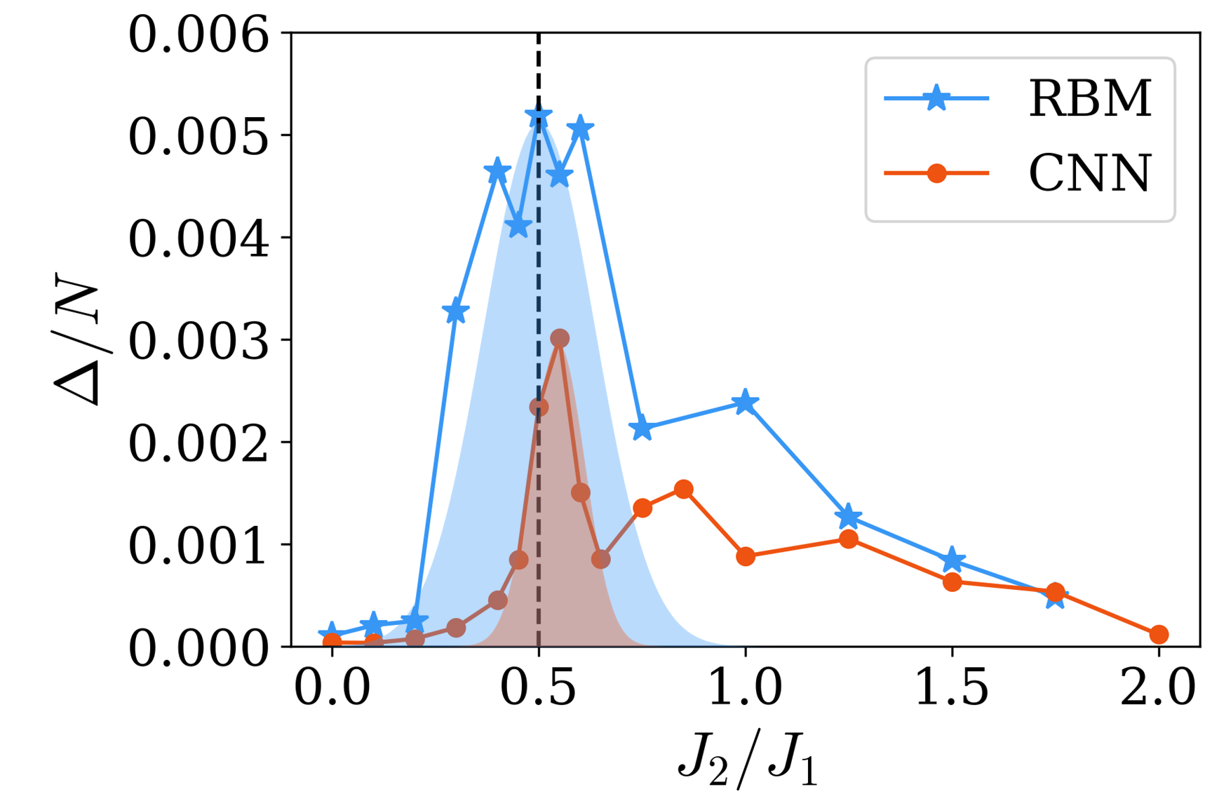
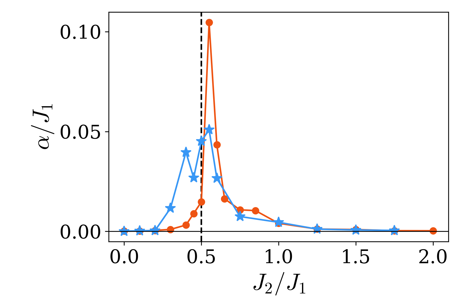
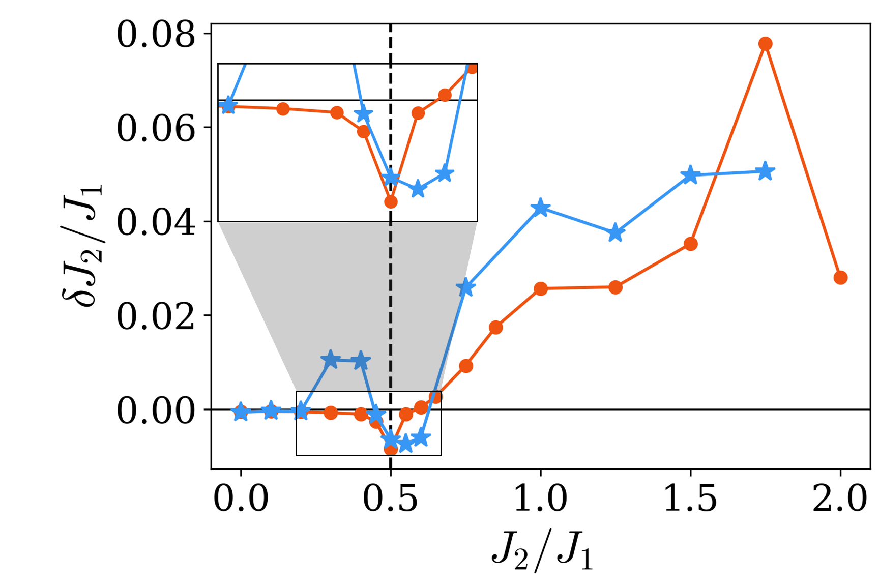
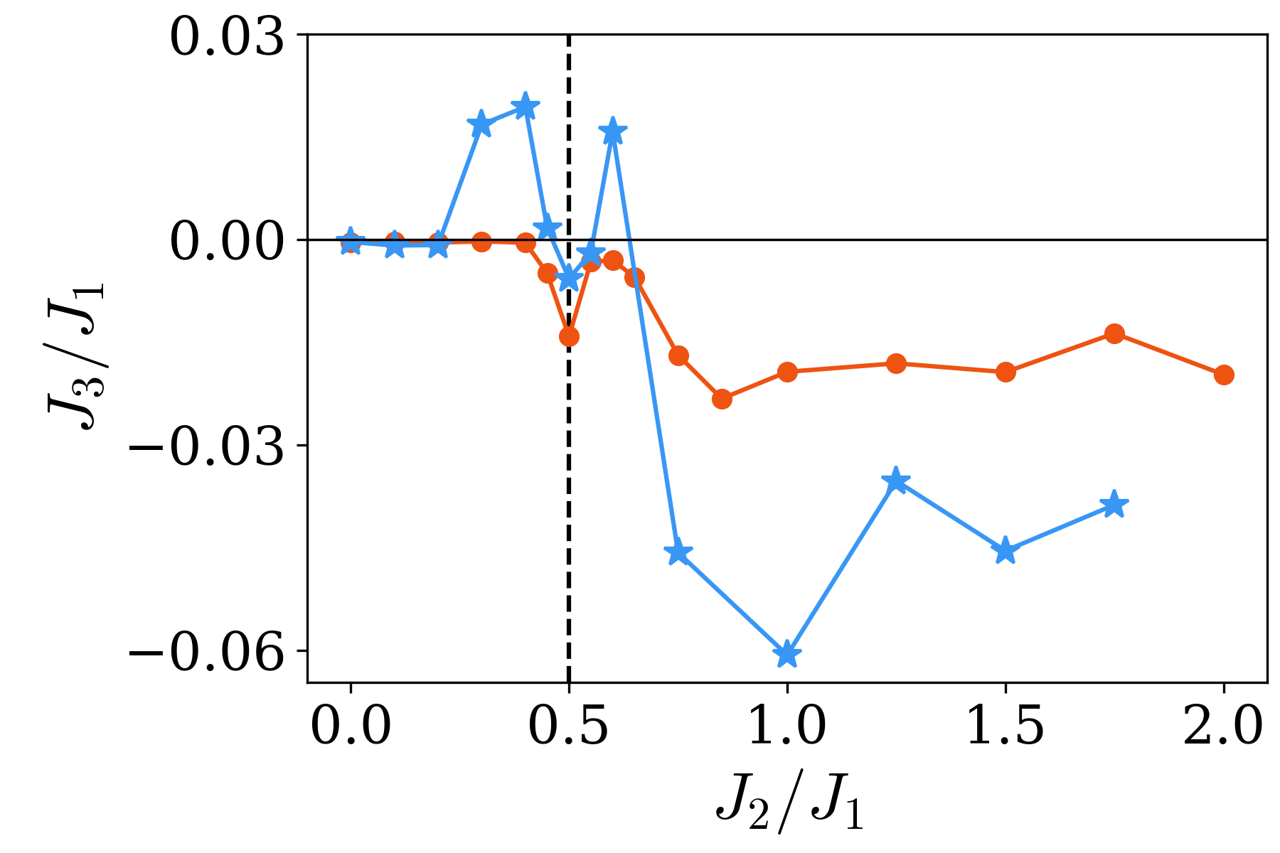
Figure 2: Ground state energy differences, and parameters of the reconstructed Hamiltonians, of CNN and RBM wavefunctions. The vertical broken line marks $J_{2}/J_{1}=0.5$, which is the classical maximum frustration point. a) Ground state energy difference (relative to true ground state obtained via exact diagonalization) per site. The shaded area is a guide to the eye that outlines the range in which the energy difference is attributable to the wavefunction anisotropy (see panel b). The unshaded energy difference in the large $J_{2}$ regime is associated with errors in the reconstructed spin couplings, panels c) and d). b) The reconstructed easy-axis anisotropy $\alpha/J_{1}$, which is primarily peaked at the classical high frustration point and dies off in the small $J_{2}$ and large $J_{2}$ limits. c) The reconstructed difference in the nearest-neighbor coupling, $\delta J_{2}/J_{1}$. The reconstruction deviates slightly from the expected value of 0 around $J_{2}=0.5$, as well as in the large $J_{2}$ regime in a more pronounced manner. d) The reconstructed longer-range interaction parameter $J_{3}/J_{1}$. Together with panel c), the reconstructions of the spin couplings $J_{2}$ and $J_{3}$ are associated with the energy differences of the trained wavefunctions outside the neighborhood of the classical high frustration point.

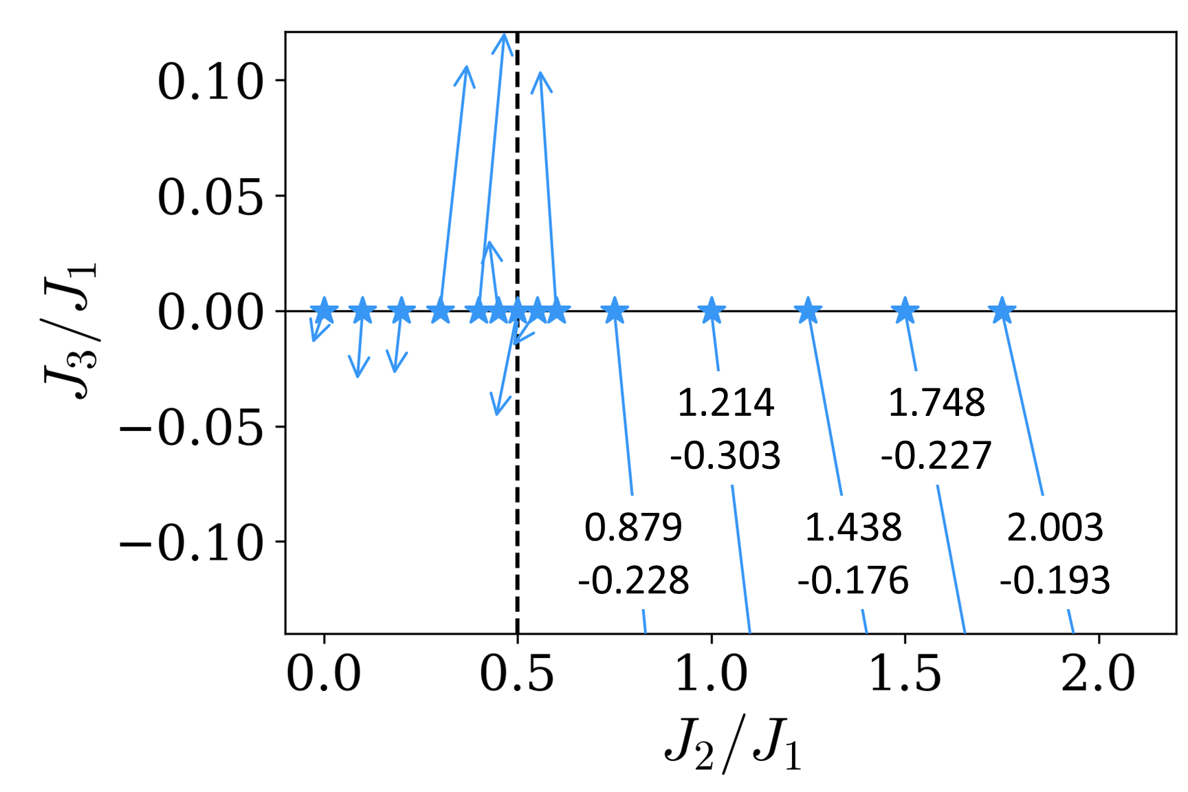
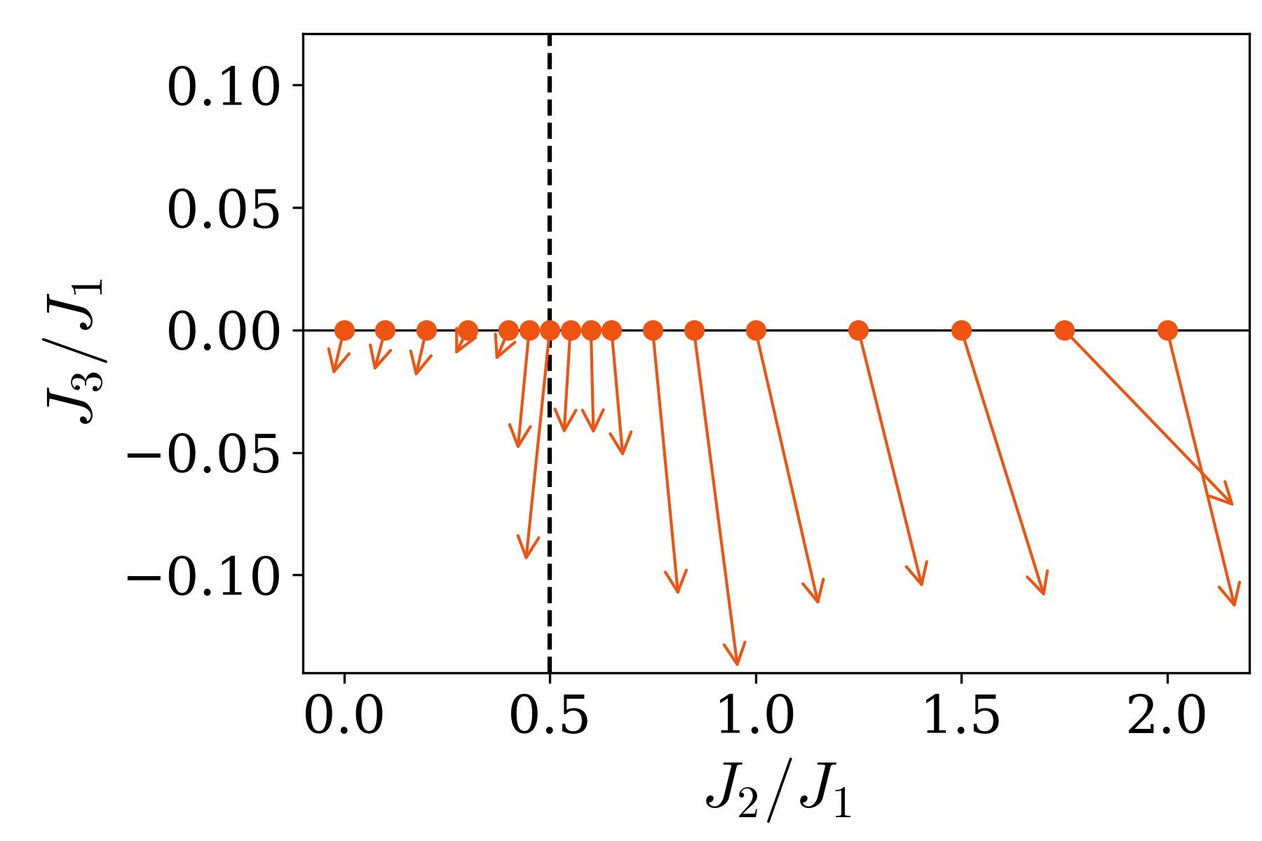
Figure 3: Schematic summary of $\delta J_{2}$ and $J_{3}$ reconstructions of (a) RBM and (b) CNN wavefunctions. The markers represent initial $J_{2}/J_{1}$ parameters for which we trained variational wavefunctions. The tips of the arrows show the reconstructed spin coupling parameters from the trained wavefunctions, i.e., $(\delta J_{2}+J_{2})/J_{1}$ and $J_{3}/J_{1}$, with the deviations magnified by a factor of 5 for clarity. The annotations beside clipped arrows describe the locations of the arrowheads (upper: $J_{2}/J_{1}$, lower: reconstructed $J_{3}/J_{1}$).

Conclusions – We have proposed Hamiltonian reconstruction as a method to probe many-body variational wavefunctions beyond their energies. Taking on the $J_{1}-J_{2}$ model and two neural network based variational wavefunctions, RBM and CNN, we investigated the Hamiltonian spaces parametrized by three channels of deviations from the target model: $\delta J_{2}$, $J_{3}$, and $\alpha$. Our results dissect the $J_{2}/J_{1}$ parameter space into two regimes: the regime dominated by frustration ($J_{2}/J_{1}\approx 0.5$) and the regime dominated by classical stripe order ($J_{2}/J_{1}>0.5$). We found the anisotropy $\alpha$ to be the dominant cause of error near the high-frustration point. Moreover, we found $\delta J_{2}$ and $J_{3}$ reconstruction to both indicate suppression of quantum fluctuation through artificial enhancement of classical order in the large $J_{2}$ regime. Overall, the Hamiltonian reconstruction revealed mutliple ways for a variational wavefunction to fail in capturing highly frustrated ground states steeped in quantum fluctuations.

Looking ahead, we expect that Hamiltonian reconstruction can be an effective means to refine variational constructions in both classical and quantum (such as variational quantum eigensolvers) platforms. With new insight into the performance of variational wavefunctions, specific areas of improvement can be identified, informing future selection of variational constructions. Further, our results concerning the $J_{1}$-$J_{2}$ model may serve as guidelines for future neural network studies of similar frustrated spin systems.

Acknowledgements. KZ, SL, and E-AK acknowledge NSF, Institutes for Data-Intensive Research in Science and Engineering – Frameworks (OAC-19347141934714). KC and TN acknowledge the European Research Council under the European Union’s Horizon 2020 research and innovation program (ERC-StG-Neupert-757867-PARATOP).

References

- Troyer and Wiese (2005) M. Troyer and U.-J. Wiese, Phys. Rev. Lett. 94, 170201 (2005).
- Verstraete et al. (2008) F. Verstraete, V. Murg, and J. Cirac, Advances in Physics 57, 143 (2008).
- Carleo and Troyer (2017) G. Carleo and M. Troyer, Science 355, 602 (2017).
- Choo et al. (2019) K. Choo, T. Neupert, and G. Carleo, Phys. Rev. B 100, 125124 (2019).
- Peruzzo et al. (2014) A. Peruzzo, J. McClean, P. Shadbolt, M.-H. Yung, X.-Q. Zhou, P. J. Love, A. Aspuru-Guzik, and J. L. O’Brien, Nature Communications 5, 10.1038/ncomms5213 (2014).
- McClean et al. (2016) J. R. McClean, J. Romero, R. Babbush, and A. Aspuru-Guzik, New Journal of Physics 18, 023023 (2016).
- Qi and Ranard (2019) X.-L. Qi and D. Ranard, Quantum 3, 159 (2019).
- Chertkov and Clark (2018) E. Chertkov and B. K. Clark, Phys. Rev. X 8, 031029 (2018).
- Bairey et al. (2019) E. Bairey, I. Arad, and N. H. Lindner, Phys. Rev. Lett. 122, 020504 (2019).
- Valenti et al. (2019) A. Valenti, E. van Nieuwenburg, S. Huber, and E. Greplova, Physical Review Research 1, 10.1103/physrevresearch.1.033092 (2019).
- Pakrouski (2020) K. Pakrouski, Quantum 4, 315 (2020).
- Dupont and Laflorencie (2019) M. Dupont and N. Laflorencie, Phys. Rev. B 99, 020202 (2019).
- Dagotto and Moreo (1989) E. Dagotto and A. Moreo, Phys. Rev. Lett. 63, 2148 (1989).
- Schulz and Ziman (1992) H. J. Schulz and T. A. L. Ziman, Europhysics Letters (EPL) 18, 355 (1992).
- Hu et al. (2013) W.-J. Hu, F. Becca, A. Parola, and S. Sorella, Phys. Rev. B 88, 060402 (2013).
- Gong et al. (2014) S.-S. Gong, W. Zhu, D. N. Sheng, O. I. Motrunich, and M. P. A. Fisher, Phys. Rev. Lett. 113, 027201 (2014).
- Jiang et al. (2012) H.-C. Jiang, H. Yao, and L. Balents, Phys. Rev. B 86, 024424 (2012).
- Sachdev and Bhatt (1990) S. Sachdev and R. N. Bhatt, Phys. Rev. B 41, 9323 (1990).
- Mambrini et al. (2006) M. Mambrini, A. Läuchli, D. Poilblanc, and F. Mila, Phys. Rev. B 74, 144422 (2006).
- Yu and Kao (2012) J.-F. Yu and Y.-J. Kao, Phys. Rev. B 85, 094407 (2012).
- Wang and Sandvik (2018) L. Wang and A. W. Sandvik, Phys. Rev. Lett. 121, 107202 (2018).
- Ferrari and Becca (2020) F. Ferrari and F. Becca, arXiv preprint arXiv:2005.12941 (2020).
- Nomura and Imada (2020a) Y. Nomura and M. Imada, arXiv preprint arXiv:2005.14142 (2020a).
- Cybenko (1989) G. Cybenko, Mathematics of Control, Signals and Systems 2, 303 (1989).
- Bishop (1995) C. Bishop, Neural Networks for Pattern Recognition (Oxford University Press, 1995).
- Deng et al. (2017) D.-L. Deng, X. Li, and S. Das Sarma, Phys. Rev. X 7, 021021 (2017).
- Nomura et al. (2017) Y. Nomura, A. S. Darmawan, Y. Yamaji, and M. Imada, Phys. Rev. B 96, 205152 (2017).
- Carleo et al. (2018) G. Carleo, Y. Nomura, and M. Imada, Nature Communications 9, 10.1038/s41467-018-07520-3 (2018).
- Chen et al. (2018) J. Chen, S. Cheng, H. Xie, L. Wang, and T. Xiang, Phys. Rev. B 97, 085104 (2018).
- Glasser et al. (2018) I. Glasser, N. Pancotti, M. August, I. D. Rodriguez, and J. I. Cirac, Phys. Rev. X 8, 011006 (2018).
- Saito and Kato (2018) H. Saito and M. Kato, Journal of the Physical Society of Japan 87, 014001 (2018).
- Choo et al. (2018) K. Choo, G. Carleo, N. Regnault, and T. Neupert, Phys. Rev. Lett. 121, 167204 (2018).
- Kochkov and Clark (2018) D. Kochkov and B. K. Clark, Variational optimization in the ai era: Computational graph states and supervised wave-function optimization (2018), arXiv:1811.12423 [cond-mat.str-el] .
- Luo and Clark (2019) D. Luo and B. K. Clark, Physical Review Letters 122, 10.1103/physrevlett.122.226401 (2019).
- Pastori et al. (2019) L. Pastori, R. Kaubruegger, and J. C. Budich, Phys. Rev. B 99, 165123 (2019).
- Sharir et al. (2020) O. Sharir, Y. Levine, N. Wies, G. Carleo, and A. Shashua, Physical Review Letters 124, 020503 (2020).
- Nomura and Imada (2020b) Y. Nomura and M. Imada, Dirac-type nodal spin liquid revealed by machine learning (2020b), arXiv:2005.14142 [cond-mat.str-el] .
- Gao and Duan (2017) X. Gao and L.-M. Duan, Nature Communications 8, 10.1038/s41467-017-00705-2 (2017).
- Levine et al. (2019) Y. Levine, O. Sharir, N. Cohen, and A. Shashua, Phys. Rev. Lett. 122, 065301 (2019).
- Carleo et al. (2019) G. Carleo, K. Choo, D. Hofmann, J. E. Smith, T. Westerhout, F. Alet, E. J. Davis, S. Efthymiou, I. Glasser, S.-H. Lin, M. Mauri, G. Mazzola, C. B. Mendl, E. van Nieuwenburg, O. O’Reilly, H. Théveniaut, G. Torlai, F. Vicentini, and A. Wietek, SoftwareX 10, 100311 (2019).
- Vieijra et al. (2020) T. Vieijra, C. Casert, J. Nys, W. De Neve, J. Haegeman, J. Ryckebusch, and F. Verstraete, Phys. Rev. Lett. 124, 097201 (2020).