One-sided Frank-Wolfe algorithms for saddle problems

Abstract

We study a class of convex-concave saddle-point problems of the form $\min_{x}\max_{y}\langle Kx,y\rangle+f_{\cal P}(x)-h^{\ast}(y)$ where $K$ is a linear operator, $f_{\cal P}$ is the sum of a convex function $f$ with a Lipschitz-continuous gradient and the indicator function of a bounded convex polytope ${\cal P}$, and $h^{\ast}$ is a convex (possibly nonsmooth) function. Such problem arises, for example, as a Lagrangian relaxation of various discrete optimization problems. Our main assumptions are the existence of an efficient linear minimization oracle (${\tt lmo}$) for $f_{\cal P}$ and an efficient proximal map (${\tt prox}$) for $h^{*}$ which motivate the solution via a blend of proximal primal-dual algorithms and Frank-Wolfe algorithms. In case $h^{*}$ is the indicator function of a linear constraint and function $f$ is quadratic, we show a $O(1/n^{2})$ convergence rate on the dual objective, requiring $O(n\log n)$ calls of ${\tt lmo}$. If the problem comes from the constrained optimization problem $\min_{x\in\mathbb{R}^{d}}\{f_{\cal P}(x)\>|\>Ax-b=0\}$ then we additionally get bound $O(1/n^{2})$ both on the primal gap and on the infeasibility gap. In the most general case, we show a $O(1/n)$ convergence rate of the primal-dual gap again requiring $O(n\log n)$ calls of ${\tt lmo}$. To the best of our knowledge, this improves on the known convergence rates for the considered class of saddle-point problems. We show applications to labeling problems frequently appearing in machine learning and computer vision.

1 Introduction

In this paper, we consider the following class of saddle-point problems:

$$\min_{x\in{\cal X}}\max_{y\in{\cal Y}}{\cal L}(x,y):=\langle{Kx},\,{y}\rangle+f_{\cal P}(x)-h^{*}(y)$$ (1)

where ${\cal X},{\cal Y}$ are finite dimensional spaces, equipped with an inner product $\langle{\cdot},\,{\cdot}\rangle$ and $K:{\cal X}\to{\cal Y}$ is a bounded linear operator with operator norm $L_{K}=\|{K}\|$. Usually the underlying spaces are the standard Euclidean spaces ${\cal X}=\mathbb{R}^{n}$ and ${\cal Y}=\mathbb{R}^{m}$.

The functions $f_{\cal P}(x)$ and $h^{*}$ are convex, lower semicontinuous functions.

For a differentiable convex function $f$ we say that it has a Lipschitz continuous gradient if there exists a constant $L_{f}\geq 0$ such that

$$\|{\nabla f(x)-\nabla f(y)}\|\leq L_{f}\|{x-y}\|,\quad\forall x,y\in{\cal X}.$$

Moreover, the function $f$ is called strongly convex with strong convexity parameter $\mu_{f}>0$ if

$$f(y)\geq f(x)+\langle{\nabla f(x)},\,{y-x}\rangle+\frac{\mu_{f}}{2}\|{y-x}\|^{2},\quad\forall x,y\in{\cal X}.$$

We make the following important structural assumptions on the functions $f_{\cal P}(x)$ and $h^{*}$:

• The function $f_{\cal P}(x)$ has the following composite form

  $$f_{\cal P}(x)=f(x)+\delta_{{\cal P}}(x),$$

  where $f$ is a convex function with a $L_{f}$-Lipschitz continuous gradient and $\delta_{{\cal P}}$ is the indicator function of a convex polytope ${\cal P}\subset{\cal X}$. For this polytope, we assume the existence of an efficient linear minimization oracle (${\tt lmo}$), which means that for any $a\in{\cal X}^{*}$, one can efficiently solve

  $${\tt lmo}_{{\cal P}}(a)\in\arg\min_{x\in{\cal P}}\langle{a},\,{x}\rangle.$$

  This is for example the case if ${\cal P}$ is the polytope arising from LP relaxations of MAP-MRF problems in a tree-structured graph, where the above problem can be solved efficiently using dynamic programming.

• The function $h^{*}$ is a convex function which allows to efficiently compute its proximal map (${\tt prox}$), which for any $\bar{y}\in{\cal Y}$ and $\tau>0$ is defined as

  $${\tt prox}_{\tau h^{*}}(\bar{y})=\arg\min_{y\in{\cal Y}}\frac{1}{2\tau}\|{y-\bar{y}}\|^{2}+h^{*}(y).$$

  Important examples of $h^{*}$ which allow for an efficient proximal map include quadratic functions and various norms. If $h^{*}=\delta_{C}$ i.e. the indicator functions of some convex set $C$ the proximal map reduces the orthogonal projection operator.

An important special case of problem (1) is given by

$$\min_{x\in\mathbb{R}^{d}}\max_{y\in\mathbb{R}^{d}}{\cal L}(x,y):=f_{\cal P}(x)+\langle{y},\,{Ax-b}\rangle$$ (2)

where $A$ is a matrix and $b$ is a vector of appropriate dimensions. This corresponds to the problem of minimizing $f_{\cal P}(x)$ subject to the linear constraint $Ax-b=0$.

Primal and dual problems   We denote by $(x^{\star},y^{\star})$ a saddle point of problem (1), which satisfies

$${\cal L}(x^{\star},y)\leq{\cal L}(x^{\star},y^{\star})\leq{\cal L}(x,y^{\star}),\quad\forall(x,y)\in{\cal X}\times{\cal Y}.$$

Throughout the paper we denote the primal and dual problems respectively by

$${F}(x)=\max_{y\in{\cal Y}}{\cal L}(x,y),\quad H(y)=\min_{x\in{\cal X}}{\cal L}(x,y).$$

We assume that strong duality holds, that is

$$H(y^{\star})=\max_{y\in{\cal Y}}H(y)=\max_{y\in{\cal Y}}\min_{x\in{\cal X}}{\cal L}(x,y)=\min_{x\in{\cal X}}{F}(x)={F}(x^{\star})$$

Some of the results will also assume coercivity of a function. We recall that a proper function $\phi(z)$ is called coercive if

$$\lim_{\|{z}\|\to\infty}\phi(z)=\infty.$$

Contributions   The algorithms we propose here are based on inexact proximal algorithms, which allow for an approximate evaluation of the proximal maps. For this we make use of efficient variants of the Frank-Wolfe algorithm that offer a linear convergence rate on the proximal subproblems. In summary, after $O(n\log n)$ calls to ${\tt lmo}$ we achieve the following guarantees.

• If function $f$ is linear or quadratic, $h^{*}$ is the indicator function of a linear constraint, and function $-H(y)$ is coercive then we obtain accuracy $O(1/n^{2})$ on the dual objective $H$. If in addition the problem has the form of eq. (2) then we obtain accuracy $O(1/n^{2})$ both on the primal gap $f_{\cal P}(x)-f_{\cal P}(x^{\star})$ and on the infeasibility gap $||Ax-b||$.

• In the most general case, we obtain accuracy $O(1/n)$ on the dual objective (and also on the primal objective assuming that $\operatorname*{dom}h^{\ast}\subseteq{\cal Y}$ is compact).

To the best of our knowledge these rates improve on the so far known rates for the class of saddle-point problems considered in this paper. In particular, for the problem in eq. (2) previous works (described later in Sec. 1.2) after $n$ calls to ${\tt lmo}$ obtained accuracy $O(1/n)$ on the dual objective and accuracy $O(1/\sqrt{n})$ on both $f_{\cal P}(x)-f_{\cal P}(x^{\star})$ and $||Ax-b||$.

1.1 Motivating example

An important application, which also serves as the main motivation for the class of saddle-point problems studied in this paper, is given by the Lagrangian relaxation of discrete optimization problems. To form such relaxation, one needs to first encode discrete variables via Boolean indicator variables $X\in\{0,1\}^{d}$, and then express a difficult optimization problem as a sum of tractable subproblems:

$$\min_{X\in\{0,1\}^{d}}\;\;\sum_{t\in T}f_{t}(X_{A_{t}})$$ (3)

Here $T=\{1,\ldots,m\}$ is the set of terms where each term $t$ is specified by a subset of variables $A_{t}\subseteq[d]$ and a function $f_{t}:\{0,1\}^{A_{t}}\rightarrow\mathbb{R}\cup\{+\infty\}$ of $|A_{t}|$ variables. Vector $X_{A_{t}}$ is the restriction of vector $X\in\mathbb{R}^{d}$ to $A_{t}$. The arity $|A_{t}|$ of function $f_{t}$ can be arbitrarily large, however we assume the existence of an efficient min-oracle that for a given vector $Y\in\mathbb{R}^{A_{t}}$ computes $X\in\operatorname*{arg\,min}\nolimits_{X\in\{0,1\}^{A_{t}}}\left[f_{t}(X)+\langle X,Y\rangle\right]$ together with the cost $f_{t}(X)$. For example, this holds if $f_{t}(\cdot)$ corresponds to a MAP-MRF inference problem in a tree-structured graph.

It is now easy to define a relaxation of (3) that will have the form of eq. (1) (see e.g. [44]). First, for each $t\in T$ let us define polytope ${\cal P}^{t}={\tt conv}(\{[X\;f(X)]\>|\>X\in\operatorname*{dom}f_{t}\})\subseteq\mathbb{R}^{A_{t}}\times R$ where $\operatorname*{dom}f_{t}=\{X\in\{0,1\}^{A_{t}}\>|\>f_{t}(X)<+\infty\}$ is the effective domain of $f_{t}$. Problem (3) can then be equivalently written as

$$\min_{X\in\{0,1\}^{d},X^{1}\in{\cal P}^{1},\ldots,X^{m}\in{\cal P}^{m}}\;\;\sum_{t\in T}X^{t}_{\circ}\qquad\quad\mbox{s.t.}\quad X_{v}=X^{t}_{v}\qquad\forall t\in T,v\in A_{t}$$ (4)

where $X^{t}_{\circ}$ denotes the last component of vector $X^{t}\in\mathbb{R}^{A_{t}}\times R$. By dropping constraint $X\in\{0,1\}^{d}$, dualizing equalities $X^{t}_{v}-X_{v}=0$ with a Lagrange multiplier $Y_{v}^{t}$, and eliminating variables $X$, we obtain the following saddle point problem which is a relaxation of (4) (its optimal value is a lower bound on (4)):

$$\min_{x=(X^{1},\ldots,X^{m})\in{\cal P}^{1}\times\ldots\times{\cal P}^{m}}\;\;\;\max_{y=(Y^{t}_{v})_{t\in T,v\in A_{t}}\in{\cal Y}}\;\;\sum_{t\in T}X^{t}_{\circ}+\sum_{t\in T,v\in A_{t}}X^{t}_{v}Y^{t}_{v}$$ (5)

where ${\cal Y}$ is the set of vectors $y=(Y^{t}_{v})_{t\in T,v\in A_{t}}$ satisfying constraints $\sum_{t:v\in A_{t}}Y^{t}_{v}=0$ for all $v\in[d]$. This problem has the form of eq. (1) where function $f(x)$ is linear and $h^{\ast}(y)$ is the indicator function of a linear constraint on $y$.

As an example, the MAP-MRF inference problem on an undirected graph can be cast in the framework above by decomposing the graph into tree-structured subproblems. It is well-known that the Lagrangian relaxation is equivalent to a standard LP relaxation, aka the local polytope relaxation [19, 34]. MAP-MRF problems find numerous applications in machine learning and computer vision [7]. In more recent work, they also appears as the final inference layer in deep convolutional neural networks [18].

1.2 Related work

Saddle point problems in the form of (1) can be solved by a large number of proximal primal-dual algorithms (see for example the recent work [10] for a very comprehensive overview) as soon as the proximal maps for both the primal and dual functions can be solved efficiently. On the other hand, Gidel et al. proposed in [13] an extension of the Frank-Wolfe algorithm to saddle-point problems $\min_{x\in{\cal X}}\max_{y\in{\cal Y}}{\cal L}(x,y)$ by assuming the existence of an efficient linear minimization oracle for the product space ${\cal X}\times{\cal Y}$ (which is assumed to be a compact set). In this paper, we are assuming the existence of an efficient linear minimization oracle just on the primal and an efficient proximal map on the dual. Therefore, our algorithms somewhat stand between the two aforementioned techniques.

Our proposed algorithms rely on the inexact accelerated proximal gradient algorithm of Aujol and Dossal [2] and the inexact primal-dual algorithm of Rasch and Chambolle [29, Section 3.1]. Note that the first method only generates a dual sequence $\{y_{n}\}$. We extend the method and the analysis to also generate a primal sequence $\{x_{n}\}$, which is needed to solve the saddle problem (1).

Several authors studied a special case of (1) given in (2), or equivalently the problem of minimizing function $f_{\cal P}(x)=f(x)+\delta_{\cal P}(x)$ subject to linear constraints $Ax=b$ [14, 23, 46]. (The last paper actually considered a more general class of saddle problems). Papers [23, 46] achieve an accuracy of $O(n^{-1/2})$ after $n$ iterations on the primal and infeasibility gaps, where [46] uses one ${\tt lmo}$ call per iteration and [23] uses $O(k^{2})$ ${\tt lmo}$ calls at $k$-th iteration assuming that a standard Frank-Wolfe method is employed. Note, the papers above do not give bounds on suboptimality gaps of the dual function $H$; instead, [14, 23] bound residuals of the augmented Lagrangian, which is not directly related to the residuals of the Lagrangian in eq. (2). A similar but slightly more general class of composite optimization problems was also recently considered in [42]. In a setting similar to our paper ($\nabla f$ is Lipschitz continuous) they show $O(n^{-1/3})$ accuracy on Lagrangian values after $n$ calls to ${\tt lmo}$.

Frank-Wolfe algorithms for saddle-point problems have also been used in [1, 22]. The former paper achieved a $O(n^{-1/2})$ convergence rate on a rather general class of constrained optimization problems. The paper [22] shares some high-level similarities with our approach (such as solving smoothed primal subproblem to a given accuracy with Frank-Wolfe), but uses a different smoothing strategy that requires both primal and dual domains to be compact. This assumption rules out many interesting applications, including the one considered in Section 1.1.

There is a large body of literature on the special case of problem (1) corresponding to Lagrangian relaxation of discrete optimization problems, see e.g. [43, 36, 16, 30, 17, 32, 38, 19, 25, 33, 24, 40, 39, 44]. Some of these methods apply only to MAP inference problems in pairwise (or low-order) graphical models, because they need to compute marginals in tree-structured subproblems [16, 17, 33] or because they explicitly exploit the fact that the relaxation can be described by polynomial many constraints [38, 25, 40, 39]. The papers [17, 32] obtained accuracy $O(1/n)$ on the dual objective after $n$ iterations, by applying accelerated gradient methods [26].

The first method that we develop can be viewed as an extension of the technique in [44], which applied an inexact proximal point algorithm (PPA) to the dual objective. In contrast to [44], we apply an accelerated version of inexact PPA, specify to which accuracy the subproblems need to be solved, and analyze the convergence rate.

1.3 Notation for approximate solutions and organization of the paper

We introduce the following notation for a function $\phi$ and accuracy $\varepsilon\geq 0$:

$$z\approx_{\varepsilon}\operatorname*{arg\,min}_{z}\phi(z)\quad \Leftrightarrow \quad\phi(z)\leq\min_{z}\phi(z)+\varepsilon$$

$$z\approx_{\varepsilon}\operatorname*{arg\,max}_{z}\phi(z)\quad \Leftrightarrow \quad\phi(z)\geq\max_{z}\phi(z)-\varepsilon$$

$$z\approx_{\varepsilon}{\tt prox}_{\tau\phi}(\bar{z})\quad \Leftrightarrow \quad z\approx_{\varepsilon}\operatorname*{arg\,min}_{z}\left[\phi(z)+\frac{1}{2\tau}||z-\bar{z}||^{2}\right]$$

The rest of the paper is organized as follows. The next section describes Frank-Wolfe algorithms for minimizing a smooth function over a convex polytope. Then in Section 3 we will present our first approach, which is based on an inexact accelerated proximal point algorithm on the dual problem. In Section 4 we present our second approach, which is based on an inexact proximal primal-dual algorithm and directly solves the saddle point problem. Preliminary numerical results are given in Section 5. To make the paper more self-contained, Appendix A discusses some important results of convex optimization. Additionally, for a better readability, the more technical proofs are all moved to Appendices B-E.

2 Frank-Wolfe algorithms

Frank-Wolfe style algorithms is a class of algorithms for minimizing functions $g_{\cal P}:{\cal X}\rightarrow\mathbb{R}$ of the form $g_{\cal P}(x)=g(x)+\delta_{\cal P}(x)$ where $g$ a convex continuously differentiable function with a Lipschitz continuous gradient and ${\cal P}$ is a convex polytope. They are typically iterative techniques that work by applying a certain procedure ${\tt FWstep}(x;g_{\cal P})\mapsto x^{\prime}$ where $g_{\cal P}$ is the objective function, and $x$ and $x^{\prime}$ are respectively the old and the new iterates with $g_{\cal P}(x^{\prime})\leq g_{\cal P}(x)$. We will apply such steps to functions $g_{\cal P}$ that change from time to time, which is why $g_{\cal P}$ is made a part of the notation.

It will be convenient to denote $g^{\downarrow}_{\cal P}(x)=g_{\cal P}(x)-\min_{x\in{\cal X}}g_{\cal P}(x)$ to be a shifted version of $g_{\cal P}$ with $\min_{x\in{\cal X}}g_{\cal P}^{\downarrow}(x)=0$. The following fact is known (see [20]). For completeness, in Appendix D.1 we give a proof of the second inequality, expanding some derivations that were omitted in the proof of [20, Theorem 2].

Lemma 1 ([20]).

For a point $\hat{x}\in{\cal P}$ denote ${\tt gap}^{\tt FW}(\hat{x};g_{\cal P})=\langle\nabla g(\hat{x}),\hat{x}-s\rangle$ where $s={\tt lmo}_{\cal P}(\nabla g(\hat{x}))$. Then

$$g^{\downarrow}_{\cal P}(\hat{x})\leq{\tt gap}^{\tt FW}(\hat{x};g_{\cal P})\leq\begin{cases}g_{\cal P}^{\downarrow}(\hat{x})+LD^{2}/2&\mbox{if }g_{\cal P}^{\downarrow}(\hat{x})>LD^{2}/2\\ D\sqrt{2L\cdot g_{\cal P}^{\downarrow}(\hat{x})}&\mbox{if }g_{\cal P}^{\downarrow}(\hat{x})\leq LD^{2}/2\end{cases}$$

where $D$ is the diameter of ${\cal P}$ and $L=L_{g}$ is the Lipschitz constant of $\nabla g$.

While the original FW algorithm has a sublinear convergence rate, there are several variants that achieve a linear convergence rate under some assumptions on $g$. Examples include Frank-Wolfe with away steps (AFW) [20], Decomposition-invariant Conditional Gradient (DiCG) [12, 3], and Blended Conditional Gradient (BCG) [8]. Each step in these methods is classified as either good or bad. Good steps are guaranteed to decrease $g_{\cal P}^{\downarrow}(x)$ by a constant factor. Bad steps do not have such guarantee (because they hit the boundary of the polytope), but they make $x$ “sparser” in a certain sense and thus cannot happen too often.

More formally, consider a class of functions $\mathfrak{F}$ where each function $g_{\cal P}\in\mathfrak{F}$ is associated with a parameter vector $\Theta_{g_{\cal P}}\in\mathbb{R}^{p}$, and ${\cal P}=\operatorname*{dom}g_{\cal P}$ is the same for all $g_{\cal P}\in\mathfrak{F}$. We say that procedure ${\tt FWstep}$ has a linear convergence rate on $\mathfrak{F}$ if there exist continuous function $\theta:\mathbb{R}^{p}\rightarrow(0,1)$ and integers $R_{0},R_{1}\geq 0$ with the following properties: (i) if the step ${\tt FWstep}(x;g_{\cal P})\mapsto x^{\prime}$ for $g_{\cal P}\in\mathfrak{F}$ is good then $g_{\cal P}^{\downarrow}(x^{\prime})\leq\theta(\Theta_{g_{\cal P}})\cdot g_{\cal P}^{\downarrow}(x)$; (ii) when applying ${\tt FWstep}(x;g_{\cal P})$ iteratively to some initial vector $x_{0}$ (possibly for different functions $g_{\cal P}\in\mathfrak{F}$), at any point we have $N_{\tt bad}\leq R_{0}+R_{1}N_{\tt good}$ where $N_{\tt good}$ and $N_{\tt bad}$ are respectively the numbers of good and bad steps.

We will consider two classes of functions:

• $\mathfrak{F}_{\tt strong}=\{g_{\cal P}(x)=g(x)+\delta_{\cal P}(x)\>:\>$ $g$ is a strongly convex differentiable function with a Lipschitz-continuous gradient, with $\Theta_{g_{\cal P}}=(\mu_{g},L_{g})$ $\}$.

• $\mathfrak{F}_{\tt weak}=\{g_{\cal P}(x)=g(Ex)+\langle b,x\rangle+\delta_{\cal P}(x)\>:\>$ $g$ is a strongly convex differentiable function with a Lipschitz-continuous gradient, and $E,b$ are matrix and vector of appropriate dimensions, with $\Theta_{g_{\cal P}}=(\mu_{g},L_{g},E,b)$ $\}$.

Note that class $\mathfrak{F}_{\tt strong}$ is implicitly parameterized by the dimension of vector $x$, and class $\mathfrak{F}_{\tt weak}$ is implicitly parameterized by the dimensions of vector $x$ and matrix $E$.

The AFW method is known to have linear convergence on $\mathfrak{F}_{\tt strong}$ [20] and also on $\mathfrak{F}_{\tt weak}$ [4, 20]. From the result of [4, 20] it is easy to deduce that the DiCG method with away steps also has linear convergence on $\mathfrak{F}_{\tt weak}$, using [3, Property 1]. The BCG method [8] has been shown to have linear convergence on class $\mathfrak{F}_{\tt strong}$.

Remark 1.

Some of the techniques above maintain some additional information about current iterate $x$. In particular, AFW and BCG represent $x$ as a convex combination of “atoms” (vertices of ${\cal P}$): $x=\sum_{i}\alpha_{i}a_{i}$ where $\alpha_{i}\geq 0$, $\sum_{i}\alpha_{i}=1$ and $a_{i}$ are atoms. Coefficients $\alpha_{i}$ are updated together with $x$. For brevity, we omitted this from the notation.

Remark 2.

The claims about the number of bad steps are proven in [20, 12, 3, 8] assuming that the function $g_{\cal P}$ is fixed. However, the proofs only use “structural” properties of current iterate $x$; they are easily extended to the case when $g_{\cal P}$ is changing, as long as ${\cal P}$ is fixed.

Iterative application of ${\tt FWstep}$   Procedure ${\tt FWstep}$ can be used in a natural way to solve problems $x\approx_{\varepsilon}\operatorname*{arg\,min}_{x}g_{\cal P}(x)$ up to desired accuracy $\varepsilon$.

1 while true do

2       update $x\leftarrow{\tt FWstep}(x;g_{\cal P})$

3       if ${\tt gap}^{\tt FW}(x;g_{\cal P})\leq\varepsilon$ then return $x$

Output: vector $x^{\prime}\approx_{\varepsilon}\operatorname*{arg\,min}_{x}g_{\cal P}(x)$.

Algorithm 1 Algorithm ${\tt FW}_{\varepsilon}(x;g_{\cal P})$.

Output: vector $x^{\prime}\approx_{\varepsilon}\operatorname*{arg\,min}_{x}g_{\cal P}(x)$.

Proposition 2.

Suppose that procedure ${\tt FWstep}$ has a linear convergence rate on class $\mathfrak{F}$ that contains $g_{\cal P}$. Then,
(a) The number of good steps made during ${\tt FW}_{\varepsilon}(x_{0};g_{\cal P})$ satisfies

$$N_{\tt good}\leq\log_{1/\theta(\Theta_{g_{\cal P}})}\frac{g^{\downarrow}_{\cal P}(x_{0})}{\min\{\frac{1}{2}LD^{2},\frac{1}{2L}\left(\frac{\varepsilon}{D}\right)^{2}\}}$$ (6)

where $D$ is the diameter of ${\cal P}$ and $L>0$ is any constant satisfying $L\geq L_{g}$.
(b) Suppose that $g_{\cal P}\in\tilde{\mathfrak{F}}\subseteq\mathfrak{F}$ where $\sup_{g_{\cal P}\in\tilde{\mathfrak{F}},x\in{\cal P}}g^{\downarrow}_{\cal P}(x)<\infty$, $\sup_{g_{\cal P}\in\tilde{\mathfrak{F}}}L_{g}<\infty$, and $\{\Theta_{g_{\cal P}}\>|\>g_{\cal P}\in\tilde{\mathfrak{F}}\}$ is a compact subset of $\mathbb{R}^{p}$. Then $N_{\tt good}=O(\log\frac{1}{\varepsilon})$ where the constant in the $O(\cdot)$ notation depends on $\tilde{\mathfrak{F}}$.

Proof.

(a)   By the definition of linear convergence, after the given number of good steps we obtain vector $x$ satisfying $g^{\downarrow}_{\cal P}(x)\leq\min\{\frac{1}{2}LD^{2},\frac{1}{2L}\left(\frac{\varepsilon}{D}\right)^{2}\}$. By Lemma 1, such $x$ satisfies ${\tt gap}^{\tt FW}(x;g_{\cal P})\leq\varepsilon$, and therefore the algorithm will immediately terminate.

(b)   Since set $\{\Theta_{g_{\cal P}}\>|\>g_{\cal P}\in\tilde{\mathfrak{F}}\}\subseteq\mathbb{R}^{p}$ is compact and function $\theta:\mathbb{R}^{p}\rightarrow(0,1)$ is continuous, there exists $\theta^{\ast}\in(0,1)$ such that $\theta(\Theta_{g_{\cal P}})\leq\theta^{\ast}$ for all $g_{\cal P}\in\tilde{\mathfrak{F}}$. Thus, all quantities present in (6) (except for $\varepsilon$) are bounded by constants for all $g_{\cal P}\in\tilde{\mathfrak{F}}$. The claim follows. ∎

3 First approach: dual proximal point algorithm

The first approach that we consider is a proximal point algorithm (PPA) applied to the dual problem:

$$\max_{y\in{\cal Y}}\left\{H(y):=\min_{x\in{\cal X}}{\cal L}(x,y)\right\}.$$

For a point $\bar{y}\in{\cal Y}$ and a smoothing parameter $\gamma>0$, we let

$${\cal L}_{\gamma,\bar{y}}(x,y)={\cal L}(x,y)-\frac{1}{2\gamma}\|{y-\bar{y}}\|^{2},$$

which can be seen as the original saddle-point problem, but with an additional proximal regularization on the dual variable. In each iteration, the PPA solves a maximization problem of the following form:

$$\hat{y}=\operatorname*{arg\,max}_{y\in{\cal Y}}\left\{H_{\gamma,\bar{y}}(y):=\min_{x\in{\cal X}}{\cal L}_{\gamma,\bar{y}}(x,y)=H(y)-\frac{1}{2\gamma}\|{y-\bar{y}}\|^{2}\right\}.$$

Based on our structure, it will be beneficial to first solve for $\hat{x}$ and then to solve for $\hat{y}$ via its proximal map, that is

$$\hat{x}=\arg\min_{x\in{\cal X}}\left\{{F}_{\gamma,\bar{y}}(x):=\max_{y\in{\cal Y}}{\cal L}_{\gamma,\bar{y}}(x,y)\right\},\quad\hat{y}=\operatorname*{arg\,max}_{y\in{\cal Y}}{\cal L}_{\gamma,\bar{y}}(\hat{x},y)={\tt prox}_{\gamma h^{*}}(\bar{y}+\gamma K\hat{x}).$$

Note that also for the smoothed saddle-point problem, strong duality holds,

$$\min_{x\in{\cal X}}{F}_{\gamma,\bar{y}}(x)=\min_{x\in{\cal X}}\max_{y\in{\cal Y}}{\cal L}_{\gamma,\bar{y}}(x,y)=\max_{y\in{\cal Y}}H_{\gamma,\bar{y}}(y),$$

and hence each step of the PPA can be equivalently written as minimizing the primal-dual gap

$$(\hat{x},\hat{y})=\operatorname*{arg\,min}_{(x,y)\in{\cal X}\times{\cal Y}}{F}_{\gamma,\bar{y}}(x)-H_{\gamma,\bar{y}}(y)$$ (7)

It is a well-known fact that the basic proximal point algorithm can be accelerated to achieve a $O(1/n^{2})$ convergence rate [15, 31], which follows from the fact that the PPA can be seen as a steepest descent on the Moreau envelope (see Appendix A), which has a Lipschitz continuous gradient and hence can be accelerated using the technique of Nesterov [26].

However, based on our general assumptions on the problem (1), we will not be able to solve the proximal subproblems (7) exactly but only up to a certain error $\varepsilon>0$ that is

$$(\hat{x},\hat{y})\approx_{\varepsilon}\operatorname*{arg\,min}_{(x,y)\in{\cal X}\times{\cal Y}}{F}_{\gamma,\bar{y}}(x)-H_{\gamma,\bar{y}}(y),$$

which clearly implies that $\hat{x}\approx_{\varepsilon}\operatorname*{arg\,min}_{x\in{\cal X}}{F}_{\gamma,\bar{y}}(x)$ as well as $\hat{y}\approx_{\varepsilon}\operatorname*{arg\,max}_{y\in{\cal Y}}H_{\gamma,\bar{y}}(y)$. However, we can still apply the recently proposed inexact accelerated proximal gradient algorithm of Aujol and Dossal [2], that can handle such approximation while still achieving an optimal $O(1/n^{2})$ convergence rate on the dual objective. Note that the original method given in [2] only generates the dual sequence $\{y_{n}\}$ but in Algorithm 2 below we also keep the primal sequence $\{x_{n}\}$ which is needed to obtain a solution of the original saddle-point problem (1). Therefore, the algorithm below can also be seen as a generalization for solving saddlepoint problems.

1 choose nonnegative sequences $\{t_{n}\}$, $\{\varepsilon_{n}\}$ so that $t_{1}=1$ and $\rho_{n}{\stackrel{{\scriptstyle\mbox{\tiny\tt~{}def~{}}}}{{=}}}t_{n-1}^{2}-t_{n}^{2}+t_{n}>0$ for all $n\geq 2$

2 choose initial point $y_{0}\in{\cal Y}$, set $\bar{y}_{0}=y_{0}$

3 for $n=1,2,\ldots$ do

4      

$$(x_{n},y_{n}) \approx_{\varepsilon_{n}} \operatorname*{arg\,min}_{(x,y)\in{\cal X}\times{\cal Y}}{F}_{\gamma,\bar{y}_{n-1}}(x)-H_{\gamma,\bar{y}_{n-1}}(y)$$ (8)

$$\bar{y}_{n} = y_{n}+\tfrac{t_{n}-1}{t_{n+1}}(y_{n}-y_{n-1})$$ (9)

Algorithm 2 Approximate accelerated proximal gradient algorithm.

In order to analyze this algorithm, let us introduce the following quantities:

$$u_{0} =y_{0},\qquad u_{n}=y_{n-1}+t_{n}(y_{n}-y_{n-1})\qquad\forall n\geq 1$$ (10)

$$A_{n} =\sum_{k=1}^{n}t_{k}\sqrt{2\gamma\varepsilon_{k}}$$ (11)

$$B_{n} =\sum_{k=1}^{n}\gamma t_{k}^{2}\varepsilon_{k}$$ (12)

$$W_{n} =t_{n}^{2}[H(y^{\star})-H(y_{n})]+\sum_{k=2}^{n}\rho_{k}[H(y^{\star})-H(y_{k-1})]$$ (13)

$$T_{n} =t_{n}^{2}+\sum_{k=2}^{n}\rho_{k}=\sum_{k=1}^{n}t_{k}$$ (14)

First, we recall the following result from [2].

Theorem 3 ([2]).

For any $n\geq 1$ there holds

$$W_{n}+\frac{1}{2\gamma}||u_{n}-y^{\star}||^{2} \leq \frac{C^{\ast}_{n}}{2\gamma}$$ (15)

where

$$C^{\ast}_{n} = ||y_{0}-y^{\star}||^{2}+2A_{n}\left(||y_{0}-y^{\star}||+2A_{n}+\sqrt{2B_{n}}\right)+2B_{n}$$ (16)

$$\leq \left(||y_{0}-y^{\star}||+2A_{n}+\sqrt{2B_{n}}\right)^{2}$$ (17)

This theorem immediately implies the following results. (Note, some of the statements below are slightly modified versions of statements from [2], but follow exactly the same proofs).

Corollary 4 ([2]).

Suppose that sequences $\{A_{n}\}$ and $\{B_{n}\}$ are bounded. Then
(a) $H(y^{\star})-H(y_{n})=O(1/t_{n}^{2})$.
(b) $H(y^{\star})-H(y^{e}_{n})=O(1/T_{n})$ where $y^{e}_{n}=(t_{n}^{2}y_{n}+\sum_{k=2}^{n}\rho_{k}y_{k-1})/T_{n}$.
(c) If function $-H(y)$ is coercive then sequence $\{y_{n}\}$ is bounded, and $||y_{n}-y_{n-1}||=O(1/t_{n})$.

Note that the rate of convergence in Corollary 4 depends on the choice of sequence $\{t_{n}\}$. These are some of the choices that have appeared in the literature:

• PPA: $t_{n}=1$ for all $n\geq 1$. Then $T_{n}=\Theta(n)$.

• Nesterov [26, 6]: $t_{n+1}=(1+\sqrt{1+4t_{n}^{2}})/2$ for $n\geq 1$. Then $t_{n}=\Theta(n)$ and $T_{n}=\Theta(n^{2})$.

• Aujol-Dossal [2]: $t_{n}=\left(\frac{n+a-1}{a}\right)^{d}$ with $d\in(0,1]$ and $a>\max\{1,(2d)^{1/d}\}$. Then $t_{n}=\Theta(n^{d})$ and $T_{n}=\Theta(n^{d+1})$.

When stating complexities, we will implicitly assume below that either the second case or the third case with $d=1$ is used, meaning that $t_{n}=\Theta(n)$ and $T_{n}=\Theta(n^{2})$.

We now generalize Theorem 3 to the situation in this section. This generalization is somewhat analogous to the generalization obtained by Tseng [45] (for a different Nesterov-type algorithm and with a different proof).

Theorem 5.

Denote $x^{e}_{n}=\sum_{k=1}^{n}t_{k}x_{k}/T_{n}$. For any $y\in{\cal Y}$ and any $n\geq 1$ there holds

$$T_{n}\left[{\cal L}(x^{e}_{n},y)-H(y^{\star})\right]+W_{n}+\frac{1}{2\gamma}||u_{n}-y||^{2} \leq \frac{C_{n}(y)}{2\gamma}$$ (18)

where

$$C_{n}(y) = ||y_{0}-y||^{2}+2A_{n}\left(||y-y^{\star}||+||y_{0}-y^{\star}||+2A_{n}+\sqrt{2B_{n}}\right)+2B_{n}$$ (19)

Note that setting $y=y^{\star}$ in Theorem 5 recovers Theorem 3, since in this case we have ${\cal L}(x^{e}_{n},y^{\star})\geq H(y^{\star})$ and $C_{n}(y^{\star})=C^{\ast}_{n}$.

Corollary 6.

Suppose that sequences $\{A_{n}\},\{B_{n}\}$ are bounded and $\operatorname*{dom}h^{\ast}\subseteq{\cal Y}$ is a compact set. Then ${F}(x^{e}_{n})-{F}(x^{\star})=O(1/T_{n})=O(1/n^{2})$.

Proof.

By the assumption of the corollary, quantity $C_{n}(y)$ is bounded for any $y\in\operatorname*{dom}h^{\ast}$ and $n\geq 1$. We also have ${F}(x^{e}_{n})=\max\limits_{y\in\operatorname*{dom}h^{\ast}}{\cal L}(x^{e}_{n},y)$ and ${F}(x^{\star})=H(y^{\star})$. The claim now follows directly from Theorem 5. ∎

Next, we analyze the special case of problem (1) corresponding to constrained optimization problem $\min_{x\in\mathbb{R}^{d}}\{f_{\cal P}(x)\>|\>Ax=b\}$.

Theorem 7.

Suppose we are in the case of the saddle problem in eq. (2). (a) There holds

$$f_{\cal P}(x^{e}_{n})-f_{\cal P}(x^{\star}) \leq \frac{C_{n}(0)}{2\gamma T_{n}}$$ (20)

$$||Ax^{e}_{n}-b|| \leq \sqrt{\frac{2\max\{f_{\cal P}(x^{\star})-f_{\cal P}(x^{e}_{n}),0\}}{\gamma T_{n}}}+\frac{\hat{C}_{n}}{\gamma T_{n}}$$ (21)

where

$$\hat{C}_{n}=||y_{0}||+A_{n}+\sqrt{||y_{0}||^{2}+2A_{n}\left(||y^{\star}||+||y_{0}-y^{\star}||+2A_{n}+\sqrt{2B_{n}}\right)+2B_{n}}$$

(b) There exists constant $\beta\geq 0$ such that for any $x\in{\cal P}$ we have $f_{\cal P}(x^{\star})-f_{\cal P}(x)\leq\beta||Ax-b||$.
(c) If sequences $\{A_{n}\}$ and $\{B_{n}\}$ are bounded then $f_{\cal P}(x^{e}_{n})-f_{\cal P}(x^{\star})=O(1/n^{2})$ and $||Ax^{e}_{n}-b||=O(1/n^{2})$.

Note that part (a) is derived directly from Theorem 5. In part (b) we crucially exploit the facts that ${\cal P}$ is a polytope, the feasible set $\{x\in{\cal P}:Ax-b=0\}$ is non-empty, and function $f$ has a bounded gradient on ${\cal P}$. Part (c) is an easy consequence of parts (a) and (b).

3.1 Overall algorithm

In this section we fix $n$, and denote $\bar{y}=\bar{y}_{n-1}$ and $\varepsilon=\varepsilon_{n}$. In order to implement Algorithm 2 for solving the saddle-point problem (1), we need to specify how to solve subproblem (2) for vector $\bar{y}$ up to accuracy $\varepsilon$:

$$(x_{n},y_{n}) \approx_{\varepsilon} \operatorname*{arg\,min}_{(x,y)\in{\cal X}\times{\cal Y}}{F}_{\gamma,\bar{y}}(x)-H_{\gamma,\bar{y}}(y)$$ (22)

We will first compute $x_{n}\approx_{\varepsilon}\operatorname*{arg\,min}_{x\in{\cal X}}{F}_{\gamma,\bar{y}}(x)$ by invoking Algorithm 1 for function ${F}_{\gamma,\bar{y}}$, and then solve for $y_{n}$ via its proximal map:

$$x_{n}={\tt FW}_{\varepsilon}(x_{n-1};{F}_{\gamma,\bar{y}})\qquad\qquad y_{n}=\operatorname*{arg\,max}_{y\in{\cal Y}}{\cal L}_{\gamma,\bar{y}}(x_{n},y)={\tt prox}_{\gamma h^{*}}(\bar{y}+\gamma Kx_{n})$$

(As we will see later, function ${F}_{\gamma,\bar{y}}$ has the form ${F}_{\gamma,\bar{y}}(x)=g(x)+\delta_{\cal P}(x)$ for some differentiable convex function $g$ with a $L_{g}$-Lipschitz continuous gradient, and so Algorithm 1 is indeed applicable). By construction, vector $x_{n}$ satisfies ${\tt gap}^{\tt FW}(x_{n};{F}_{\gamma,\bar{y}})\leq\varepsilon$. The following lemma thus implies that the pair $(x_{n},y_{n})$ indeed solves problem (22).

Lemma 8.

Suppose that $\hat{x}\in{\cal P}$ and $\hat{y}=\operatorname*{arg\,max}_{y}{\cal L}_{\gamma,\bar{y}}(\hat{x},y)$. Then $H_{\gamma,\bar{y}}(\hat{y})\geq{\cal L}_{\gamma,\bar{y}}(\hat{x},\hat{y})-\varepsilon={F}_{\gamma,\bar{y}}(\hat{x})-\varepsilon$ where $\varepsilon={\tt gap}^{\tt FW}(\hat{x};{F}_{\gamma,\bar{y}})$.

Next, we derive an explicit expression for function ${F}_{\gamma,\bar{y}}$ (which is needed for implementing the call $x_{n}={\tt FW}_{\varepsilon}(x_{n-1};{F}_{\gamma,\bar{y}})$), and formulate sufficient conditions on ${\cal L}$ that will guarantee that ${F}_{\gamma,\bar{y}}\in\mathfrak{F}_{\tt weak}$ (this would yield a good bound on the complexity of Algorithm 2).

Recall that the function ${F}_{\gamma,\bar{y}}(x)$ is given by

$${F}_{\gamma,\bar{y}}(x)=\max_{y\in{\cal Y}}{\cal L}_{\gamma,\bar{y}}(x,y)=\max_{y\in{\cal Y}}\langle{Kx},\,{y}\rangle+f_{{\cal P}}(x)-h^{\ast}(y)-\frac{1}{2\gamma}\|{y-\bar{y}}\|^{2}.$$

We now show that it can be written as

$${F}_{\gamma,\bar{y}}(x)=f_{{\cal P}}(x)+h_{\gamma,\bar{y}}(Kx)$$

with $h_{\gamma,\bar{y}}(Kx)$ a differentiable function with Lipschitz continuous gradient.

Lemma 9.

Let the function $h_{\gamma,\bar{y}}(Kx)$ be defined as

$$h_{\gamma,\bar{y}}(Kx)=\max_{y\in{\cal Y}}\langle{Kx},\,{y}\rangle-h^{\ast}(y)-\frac{1}{2\gamma}\|{y-\bar{y}}\|^{2}.$$

We have the following two representations:

$$h_{\gamma,\bar{y}}(Kx) = \frac{\gamma}{2}\|{Kx}\|^{2}+\langle{Kx},\,{\bar{y}}\rangle-m_{h^{*}}^{\gamma}(\bar{y}+\gamma Kx),$$ (23)

$$= m_{h}^{\gamma^{-1}}\left(\gamma^{-1}\bar{y}+Kx\right)-\frac{1}{2\gamma}\|{\bar{y}}\|^{2}.$$ (24)

where $m_{h^{*}}^{\gamma}$ is the Moreau envelope of $h^{*}$ with smoothing parameter $\gamma$ and $m_{h}^{\gamma^{-1}}$ is the Moreau envelope of $h$ with smoothing parameter $\gamma^{-1}$.
Moreover, the function $h_{\gamma,\bar{y}}(Kx)$ is convex, continuously differentiable in $x$ with a $\gamma L_{K}^{2}$-Lipschitz continuous gradient given by

$$\nabla_{x}h_{\gamma,\bar{y}}(Kx) = K^{*}{\tt prox}_{\gamma h^{*}}\left(\bar{y}+\gamma Kx\right),$$ (25)

$$= \gamma K^{*}\left(\gamma^{-1}\bar{y}+Kx-{\tt prox}_{\gamma^{-1}h}\left(\gamma^{-1}\bar{y}+Kx\right)\right).$$ (26)

In practical applications, we will mostly be interested in the situation where $h^{*}$ is a linear constraint.

Lemma 10.

Let ${\cal X}={\cal Y}=\mathbb{R}^{\ell}$, and let $h^{*}(y)=\delta_{S}(y)$ be a linear constraint of the form $S=\{y\in\mathbb{R}^{\ell}:Cy=d\}$ for some matrix $C$ with full row rank and vector $d$. Then, the function $h_{\gamma,\bar{y}}(Kx)$ is a quadratic function of the form

$$h_{\gamma,\bar{y}}(Kx)=\frac{\gamma}{2}\|{Kx}\|^{2}+\langle{Kx},\,{\bar{y}}\rangle-\frac{1}{2\gamma}\|{C^{*}(CC^{*})^{-1}(d-C(\bar{y}+\gamma Kx))}\|^{2}.$$

Moreover, its gradient is a linear map given by

$$\nabla_{x}h_{\gamma,\bar{y}}(Kx)=K^{*}\left(\bar{y}+\gamma Kx+C^{*}(CC^{*})^{-1}(d-C(\bar{y}+\gamma Kx))\right).$$

We therefore obtain the following sufficient condition where the functions ${F}_{\gamma,\bar{y}}(x)$ for any $\bar{y}\in{\cal Y}$ and any $\gamma>0$ fall into the class $\mathfrak{F}_{\tt weak}$.

Lemma 11.

Let $f(x)$ be a quadratic function of the form $f(x)=\frac{1}{2}\langle{Qx},\,{x}\rangle+\langle{q},\,{x}\rangle$, with a symmetric positive semidefinite matrix $Q$ and vector $q$. Furthermore, let $h^{*}$ satisfy the condition of Lemma 10. Then $\{{F}_{\gamma,\bar{y}}\>|\>\bar{y}\in{\cal Y}\}\subseteq\mathfrak{F}_{\tt weak}$.

Proof.

First note that both $f(x)$ and $h_{\gamma,\bar{y}}(Kx)$ are quadratic functions. By completing the squares and ignoring constant terms, it follows that ${F}_{\gamma,\bar{y}}(x)$ can be written as ${F}_{\gamma,\bar{y}}(x)=\frac{1}{2}\|{Ex}\|^{2}+\langle{b},\,{x}\rangle+\delta_{{\cal P}}(x)$ for some matrix $E$ and vector $b$, where matrix $E$ may depend on $\gamma$ but not on $\bar{y}$. ∎

It remains to specify how to set the sequence $\{\varepsilon_{n}\}$. We want sequences $\{A_{n}\}$ and $\{B_{n}\}$ to be bounded; this can be achieved by setting $\varepsilon_{n}=\Theta(n^{-4-\delta})$ for some $\delta>0$. With these choices, we obtain the main result of this section:

Theorem 12.

Suppose that function ${\cal L}$ satisfies the precondition of Lemma 11, function $-H(y)$ is coercive, and procedure ${\tt FWstep}$ has a linear convergence rate on $\mathfrak{F}_{\tt weak}$ (e.g. it is one step of AFW or DiCG). Then Algorithm 2 makes $O(n\log n)$ calls to ${\tt FWstep}$ during the first $n$ iterations, and obtains iterates $x_{n}^{e}$ and $y_{n}^{e}$ satisfying $H(y^{\star})-H(y^{e}_{n})=O(1/n^{2})$. Furthermore, in the case of the problem in eq. (2) the iterates satisfy $f_{\cal P}(x^{e}_{n})-f_{\cal P}(x^{\star})=O(1/n^{2})$ and $||Ax_{n}^{e}-b||=O(1/n^{2})$.

Proof.

By Lemma 11, all functions ${F}_{\gamma,\bar{y}_{n-1}}$ encountered during the algorithm belong to $\mathfrak{F}_{\tt weak}$. Furthermore, vectors $\bar{y}_{n-1}$ for $n\geq 1$ belong to a compact set, since the sequence $\{y_{n}\}$ (and thus the sequence $\{\bar{y}_{n}\}$) is bounded by Corollary 4(c). By Proposition 2(b) the number of good FW steps during $n$-th iteration is $O(\log\frac{1}{\varepsilon_{n}})=O(\log n)$, and during the first $n$ iterations is $\sum_{k=1}^{n}O(\log k)=O(n\log n)$. The number of bad FW steps is thus also $O(n\log n)$ by the definition of linear convergence and by the fact that the call $x_{n}={\tt FW}_{\varepsilon_{n}}(x_{n-1};{F}_{\gamma,\bar{y}_{n-1}})$ is initialized with vector $x_{n-1}$. The remaining claims follow from Corollaries 4 and 6 and Theorem 7. ∎

4 Second approach: primal-dual proximal algorithm

In this section we consider solving (1) without the restriction that $h^{*}$ is the indicator function of a linear constraint. Therefore we make use of proximal primal-dual algorithms such as [9] which in each step of the algorithm need to compute proximal maps with respect to $f_{\cal P}$ and $h^{*}$. By our problem assumptions, the proximal map with respect to $h^{*}$ is tractable but the proximal map with respect to $f_{\cal P}$ requires to solve for any $\bar{x}\in{\cal X}$ and $\tau>0$ an optimization problem of the form

$${\tt prox}_{\tau f_{\cal P}}(\bar{x})=\operatorname*{arg\,min}_{x\in{\cal P}}f(x)+\frac{1}{2\tau}\|{x-\bar{x}}\|^{2}.$$

We note the obvious fact that each proximal subproblem is a $\tau^{-1}$-strongly convex function with $L_{f}+\tau^{-1}$-Lipschitz continuous gradient over a convex polytope. Hence, it falls into the class $\mathfrak{F}_{\tt strong}$, on which Frank-Wolfe algorithms achieve a linear rate of convergence. Similar to the previous section, we will not be able to solve the subproblems exactly but up to a certain accuracy $\varepsilon>0$. We therefore need to resort to the recently proposed inexact primal-dual algorithm by Rasch and Chambolle [29, Section 3.1] which can handle such inaccuracy. The algorithm adapted to our situation is given below as Algorithm 3.

1 choose $\tau,\sigma>0$ such that $\sigma\tau L_{K}^{2}<1$

2 choose initial points $x_{0}\in{\cal X}$ and $y_{0}\in{\cal Y}$, set $x_{-1}=x_{0}$

3 for $n=0,1,\ldots$ do

4      

$$y_{n+1} = {\tt prox}_{\sigma h^{\ast}}(y_{n}+\sigma K(2x_{n}-x_{n-1}))$$ (27)

$$x_{n+1} \approx_{\varepsilon_{n+1}} {\tt prox}_{\tau f_{\cal P}}(x_{n}-\tau K^{\ast}y_{n+1})$$ (28)

Algorithm 3 Inexact primal-dual algorithm.

The following result has been shown in [29]. 

Theorem 13 ([29]).

(a) Define $x^{e}_{n}=\frac{1}{n}\sum_{k=1}^{n}x_{k}$ and $y^{e}_{n}=\frac{1}{n}\sum_{k=1}^{n}y_{k}$. Then for any $n\geq 1$ and $(x,y)\in{\cal X}\times{\cal Y}$

$${\cal L}(x_{n}^{e},y)-{\cal L}(x,y_{n}^{e})\leq\frac{1}{n}\left(\frac{||x-x_{0}||^{2}}{2\tau}+\frac{||y-y_{0}||^{2}}{2\sigma}+\frac{{\tt diam}({\cal P})}{\tau}A_{n}+\frac{1}{\tau}B_{n}\right)$$

where

$$A_{n} =\sum_{k=1}^{n}\sqrt{2\tau\varepsilon_{k}} B_{n} =\sum_{k=1}^{n}\tau\varepsilon_{k}$$ (29)

(b) If sequences $\{A_{n}\}$ and $\{B_{n}\}$ are bounded then there exists saddle point $(x^{\star},y^{\star})$ of problem (1) such that $x_{n}\rightarrow x^{\star}$ and $y_{n}\rightarrow y^{\star}$.

To solve the subproblem in eq. (3), we call Algorithm 1 via

$$x_{n+1}\leftarrow{\tt FW}_{\varepsilon_{n+1}}(x_{n};g_{n}),\qquad g_{n}(x)=f_{\cal P}(x)+\frac{1}{2\tau}||x-(x_{n}-\tau K^{\ast}y_{n+1})||^{2}$$

To make sequences $\{A_{n}\}$ and $\{B_{n}\}$ bounded, we can set $\varepsilon_{n}=\Theta(n^{-2-\delta})$ for some $\delta>0$. With these choices, we obtain

Theorem 14.

Suppose that procedure ${\tt FWstep}$ has a linear convergence rate on $\mathfrak{F}_{\tt strong}$ (e.g. it is one step of AFW, DiCG or BCG). Then Algorithm 3 makes $O(n\log n)$ calls to ${\tt FWstep}$ during the first $n$ iterations, and obtains iterates $x_{n}^{e}$ and $y_{n}^{e}$ satisfying $F(x^{e}_{n})-F(x^{\star})=O(1/n)$ (if $\operatorname*{dom}h^{\ast}$ is a compact set) and $H(y^{\star})-H(y^{e}_{n})=O(1/n)$.

Proof.

Clearly, all proximal subproblems $g_{n}$ encountered during the algorithm belong to $\mathfrak{F}_{\tt strong}$. Furthermore, vectors $\bar{x}_{n+1}{\stackrel{{\scriptstyle\mbox{\tiny\tt~{}def~{}}}}{{=}}}x_{n}-\tau K^{\ast}y_{n+1}$ for $n\geq 0$ belong to a compact set (by Theorem 13(b)). By Proposition 2(b) the number of good FW steps during $n$-th iteration is $O(\log\frac{1}{\varepsilon_{n+1}})=O(\log n)$, and during the first $n$ iterations is $\sum_{k=1}^{n}O(\log k)=O(n\log n)$. The number of bad FW steps is thus also $O(n\log n)$ by the definition of linear convergence.

Now assume that $\operatorname*{dom}h^{\ast}$ is a compact set, and define $x\in\operatorname*{arg\,min}\limits_{x\in{\cal P}}{\cal L}(x,y^{e}_{n})$, $y\in\operatorname*{arg\,max}\limits_{y\in\operatorname*{dom}h^{\ast}}{\cal L}(x^{e}_{n},y)$. We have $F(x^{e}_{n})-F(x^{\star})={\cal L}(x^{e}_{n},y)-F(x^{\star})\leq{\cal L}(x^{e}_{n},y)-H(y^{e}_{n})={\cal L}(x^{e}_{n},y)-{\cal L}(x,y^{e}_{n})$, so applying Theorem 13(a) for $(x,y)$ gives $F(x^{e}_{n})-F(x^{\star})=O(1/n)$.

It remains to prove the last claim. Since the sets $\{x_{n}\}$ and $\{y_{n}\}$ are bounded, we can assume w.l.o.g. that $\operatorname*{dom}h^{\ast}$ is a compact set (we can add indicator function $\delta_{S}(y)$ to $h^{\ast}(y)$ for a suitable set $S\subseteq{\cal Y}$ so that the algorithm and values $H(y^{\star})$, $H(y^{e}_{n})$ are not affected). Using the same argument as before, we obtain $H(y^{\star})-H(y^{e}_{n})=O(1/n)$. ∎

5 Numerical Results

(a) “Vapnik” ($200\times 150$, $50$ labels)

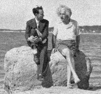
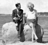
(b) “Einstein” ($200\times 185$, $50$ labels)

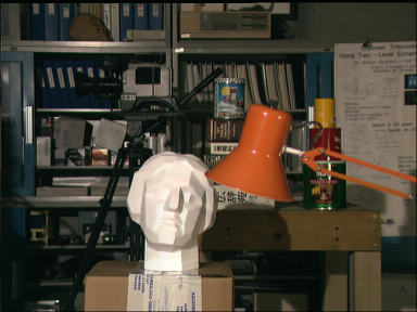
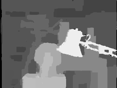
(c) “Tsukuba” ($385\times 288$, $16$ labels)

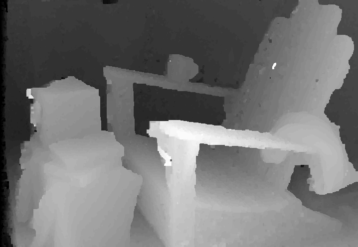
(d) “Adirondack” ($718\times 496$, $64$ labels)

Figure 1: Results of the proposed algorithm for MRF-based image denoising (first row) and disparity estimation (second row)

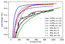
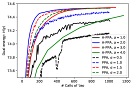
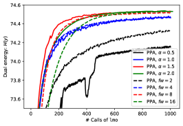
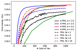
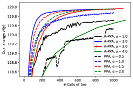
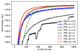
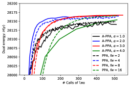
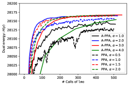
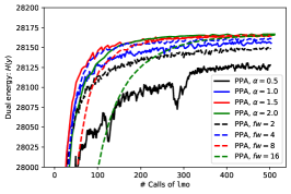
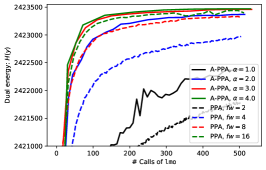
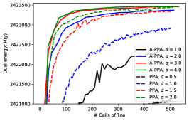
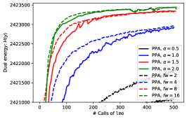
Figure 2: Convergence plots of the dual energy for “Vapnik” (first row), ”Einstein” (second row), “Tsukuba” (third row) and “Adirondack” (fourth row). See the text for more details.

In this section, we show preliminary results for solving MRFs arising from computer vision. The goal is to solve the following discrete minimization problem:

$$\min_{\mbox{\footnotesize X}\in D^{\cal V}}\;E(\mbox{X}):=\sum_{i\in{\cal V}}\theta_{i}(\mbox{X}_{i})+\sum_{ij\in{\cal E}}\theta_{ij}(\mbox{X}_{i},\mbox{X}_{j})$$

where $({\cal V},{\cal E})$ is a 4-connected 2D grid graph, $D$ is a finite set of labels, and $\theta_{i}(\cdot),\theta_{ij}(\cdot,\cdot)$ are given unary and pairwise costs, respectively. We decompose the problem into horizontal and vertical chains, and convert it to the saddle point problem (1) as described in Section 1.1.

We compare two versions of Algorithm 2: accelerated proximal point algorithm (denoted as A-PPA) with the aggressive choice $t_{n}=(n+1)/2$ (which corresponds to the Aujol-Dossal scheme with $d=1,a=2$), and the standard proximal point algorithm (denoted as PPA) which is realized by setting $t_{n}=1$. Their convergence rates after $n$ iterations are $O(1/n^{2})$ and $O(1/n)$ respectively, assuming that sequences $\{A_{n}\}$ and $\{B_{n}\}$ are bounded. We invoke Algorithm 1 to minimize the functions $F_{\gamma,\bar{y}}$ up to accuracy

$$\varepsilon_{n}={\tt gap}_{0}\cdot n^{-\alpha},$$ (30)

for a constant $\alpha>0$, where ${\tt gap}_{0}$ denotes the initial gap of the function $F_{\gamma,\bar{y}}$. Note that for $O(1/n^{2})$ convergence rate for A-PPA we would have to set $\alpha>4$, but in practice smaller settings of $\alpha$ give larger speedups.

The smoothing parameter $\gamma$ is chosen by hand, but as a general rule of thumb, it should be adapted to the scale of the primal respectively dual cost functions. Note that the selection of an optimal value of $\gamma$ is beneficial mainly from a practical point of view as it does not influence the asymptotic convergence rate. We leave the selection of an optimal value of $\gamma$ for future work.

In the case of PPA we tested two different versions. The first version is the method proposed in [44]. It uses a fixed number of Frank-Wolfe steps and is hence denoted as PPA-fw. The second version is motivated from our analysis for the case $t_{n}=1$. It uses (30) for determining the accuracy of the subproblems and hence we denote it by PPA-$\alpha$. Note that in order to guarantee an $O(1/n)$ convergence of PPA, one needs $\alpha>2$ but as before, smaller values yield larger speedups.

Procedure ${\tt FWstep}$ was implemented as follows. We explicitly maintain the current iterate $x$ as a convex combination of atoms. In the beginning of ${\tt FWstep}$ we first run a standard Frank-Wolfe step, and then re-optimize the objective over the current set of atoms. For that one needs to solve a low-dimensional strongly convex, quadratic subproblem over the unit simplex; we used the linearly converging accelerated proximal gradient method described in [27]. The resulting method can be viewed as a version of the BCG method [8], which is known to be linearly convergent on $\mathfrak{F}_{\tt strong}$.

Remark 3.

Note that there is an extensive literature on FW variants. Potential alternatives to the method above include BCFW [21] and its variants [41, 28], DiCG [12, 3], and Frank-Wolfe with in-face directions [11]. However, testing different Frank-Wolfe methods is outside the scope of this paper; instead, we study what is the best way to use a given FW method.

Next, we describe the two vision applications that we used.

Image denoising   The first application is a simple Gaussian image denoising problem. The unary terms are given by a quadratic potential function and the pairwise terms are given by a truncated quadratic potential function. Hence, this model resembles a discrete version of the celebrated Mumford-Shah functional. Figure 1 (a) and (b) show the noisy input images together with their denoised versions. The value of $\gamma$ was set to $\gamma=1e-03$ in both cases.

Stereo   The second application is a classical disparity estimation problem from rectified stereo image pairs [35]. Figure 1 (c) and (d) show the left input images together with the estimated disparity images. For the “Tsukuba” image, the unaries are computed based on the absolute color differences between the left and right input image. The unaries of the “Adirondack” image are computed using a CNN-based correlation network [18]. In bother cases the pairwise costs are given by a truncated absolute potential function. The value of $\gamma$ was set to $\gamma=1e-01$ in the case of “Tsukuba”, and $\gamma=1.0$ in the case of “Adirondack”.

Results   In Figure 2 we provide convergence plots of the three different algorithms: A-PPA, PPA-fw and PPA-$\alpha$ on all 4 examples. We plot the convergence of the dual energy $H(y)$ over the total number of calls of ${\tt lmo}$.

The plots show that A-PPA systematically outperforms both the baseline method PPA-fw (first column) as well as its variant PPA-$\alpha$ (second column). The results also indicate that the choice of $\alpha$ significantly influences the global convergence behavior. For example in Figure 2 (a) $\alpha=2$ yields the largest speedup in the first iterations but is catched up by $\alpha=3$ in later iterations of the algorithm. This suggest, that a more flexible sequence $\varepsilon_{n}$ has the potential for an additional speedup but such a development is left for future research.

From the plots in the third column one can also observe that the new variant PPA-$\alpha$ has a small speedup over the existing baseline method PPA-fw. This can be seen as a byproduct of our novel analysis in the case $t_{n}=1$. Here one can also observe that values of $\alpha<2$ yield the fastest convergence in the first iterations of the algorithm.

From a practical point of view, the plots show that $\alpha$ should be chosen according to the desired accuracy of the solution. This is of particular interest if one is only interested in a fast approximate solution to the problem, for example if the MRF is used as the last inference layer in a CNN.

6 Conclusion

In this work, we have proposed new primal-dual algorithms based on a mixture of proximal and Frank-Wolfe algorithms to solve a class of convex-concave saddle point problems arising in Lagrangian relaxations of discrete optimization problems. As our main result, we have shown after $O(n\log n)$ calls to ${\tt lmo}$ a $O(1/n)$ convergence rate in the most general case (Alg. 3) and a $O(1/n^{2})$ convergence rate with certain regularity assumptions on the dual objective (Alg. 2). To the best of our knowledge, this improves on the known rates from the literature. Our preliminary numerical results also show an improved practical performance of Alg. 2 on MAP inference problems in computer vision. Note, we have not implemented yet Alg. 3 since its rate is worse on the application that we consider; at the moment the primary purpose of Alg. 3 is to show which rates are achievable for different classes of saddle point problems.

Appendix A Some results from convex optimization

In order to make the paper more self-contained, we recall here some well-known definitions and results from convex optimization, which will be useful later. The results with their proofs can for example be found in the recent monograph by Amir Beck [5].

The convex conjugate $f^{*}$ of an extended real valued function $f$ is defined as

$$f^{*}(y)=\sup_{x}\langle{x},\,{y}\rangle-f(x),$$ (31)

which, since being a pointwise maximum over linear affine functions, is a convex lower semicontinuous function.

The infimal convolution between two proper functions $f$ and $g$ (written as $f\square g$) is defined by

$$(f\square g)(x)=\inf_{u}f(u)+g(x-u)=\inf_{x=u+v}f(u)+g(v).$$ (32)

which itself is a convex function, if $f$ is proper and convex, and $g$ is convex and real valued.

The infimal convolution and the convex conjugate for two proper functions $f,g$ are related via

$$(f\square g)^{*}=f^{*}+g^{*}.$$ (33)

Moreover, assuming that $f$ is proper and convex and $g$ is a real-valued convex function, one also has that

$$(f+g)^{*}=f^{*}\square g^{*}.$$ (34)

The Moreau envelope of a convex function $f$ with smoothness parameter $\mu>0$ is the infimal convolution of $f$ with $\mu^{-1}$ times a quadratic function.

$$m^{\mu}_{f}(x)=\inf_{x=u+v}f(u)+\frac{1}{2\mu}\|{v}\|^{2}=\left(f\square\frac{1}{2\mu}\|{\cdot}\|^{2}\right)(x).$$ (35)

Its unique minimizing argument is precisely given by the proximal map

$$\operatorname*{arg\,min}_{u}f(u)+\frac{1}{2\mu}\|{x-u}\|^{2}={\tt prox}_{\mu f}(x),$$ (36)

so that the Moreau envelope can explicitly be written as

$$m^{\mu}_{f}(x)=f({\tt prox}_{\mu f}(x))+\frac{1}{2\mu}\|{x-{\tt prox}_{\mu f}(x)}\|^{2}.$$ (37)

It is a well-known fact (and it easily follows from the monotonicity of the subdifferential), that the proximal map is a firmly nonexpansive operator, that is for any proper, convex lower semicontinuous function $f$ it holds that

$$\|{{\tt prox}_{f}(x)-{\tt prox}_{f}(y)}\|^{2}\leq\langle{{\tt prox}_{f}(x)-{\tt prox}_{f}(y)},\,{x-y}\rangle,\quad\forall x,y.$$ (38)

Furthermore, from the Cauchy-Schwartz inequality it also follows that the proximal map is a nonexpansive operator

$$\|{{\tt prox}_{f}(x)-{\tt prox}_{f}(y)}\|\leq\|{x-y}\|,\quad\forall x,y.$$ (39)

The Moreau envelop is continuously differentiable with an explicit representation of the gradient in terms of its proximal map

$$\nabla m^{\mu}_{f}(x)=\frac{1}{\mu}(x-{\tt prox}_{\mu f}(x)).$$ (40)

Furthermore, the gradient of the Moreau envelope is Lipschitz continuous with parameter $\mu^{-1}$.

The next computation (which makes use of some results above) shows the relation between the Moreau envelopes of a convex function $f$ and its convex conjugate $f^{*}$.

$$m^{\mu}_{f}(x)= \inf_{u}f(u)+\frac{1}{2\mu}\|{x}\|^{2}-\frac{1}{\mu}\langle{x},\,{u}\rangle+\frac{1}{2\mu}\|{u}\|^{2}$$

$$= \frac{1}{2\mu}\|{x}\|^{2}-\frac{1}{\mu}\sup_{u}\langle{x},\,{u}\rangle-\mu f(u)-\frac{1}{2}\|{u}\|^{2}$$

$$= \frac{1}{2\mu}\|{x}\|^{2}-\frac{1}{\mu}\left(\mu f(u)+\frac{1}{2}\|{\cdot}\|^{2}\right)^{*}(x)$$

$$= \frac{1}{2\mu}\|{x}\|^{2}-\left(f^{*}\square\frac{\mu}{2}\|{\cdot}\|^{2}\right)\left(\frac{x}{\mu}\right),$$

from which it follows the beautiful relation

$$\frac{1}{2\mu}\|{x}\|^{2}=m^{\mu}_{f}(x)+m^{\mu^{-1}}_{f^{*}}\left(\frac{x}{\mu}\right).$$ (41)

Now, taking the gradient with respect to $x$ on both sides and multiplying by $\mu$, recovers the celebrated Moreau identity

$$x={\tt prox}_{\mu f}(x)+\mu{\tt prox}_{\frac{1}{\mu}f^{*}}\left(\frac{x}{\mu}\right).$$ (42)

Appendix B Analysis of Algorithm 2: proof of Theorem 5

B.1 Proof preliminaries

We first state a few technical results the will be used in the proof of Theorem 5.

Lemma 15.

Suppose that $(\hat{x},\hat{y})\approx_{\varepsilon}\operatorname*{arg\,min}_{x,y}[F_{\gamma,\bar{y}}(x)-H_{\gamma,\bar{y}}(y)]$. Then $\hat{y}\approx_{\varepsilon-\delta}\operatorname*{arg\,max}_{y}{\cal L}_{\gamma,\bar{y}}(\hat{x},y)$ where $\delta={\cal L}(\hat{x},\hat{y})-H(\hat{y})\geq 0$.

Proof.

The claim follows from the following inequalities:

$$\max_{y}{\cal L}_{\gamma,\bar{y}}(\hat{x},y)-{\cal L}_{\gamma,\bar{y}}(\hat{x},\hat{y})=F_{\gamma,\bar{y}}(\hat{x})-{\cal L}_{\gamma,\bar{y}}(\hat{x},\hat{y})=F_{\gamma,\bar{y}}(\hat{x})-H_{\gamma,\bar{y}}(\hat{y})-\delta\leq\varepsilon-\delta$$

∎

Lemma 16 ([37, Lemma 2],[2, Lemma 2.5]).

Suppose that $\hat{y}\approx_{\varepsilon}{\tt prox}_{\gamma\phi}(\bar{y})$ for a proper convex l.s.c. function $\phi$. Then there exists $r$ with $||r||\leq\sqrt{2\gamma\varepsilon}$ such that

$$\phi(z)\geq\phi(\hat{y})+\left\langle\frac{\bar{y}-\hat{y}-r}{\gamma},z-\hat{y}\right\rangle-\varepsilon\qquad\qquad\forall z\in{\cal Y}$$

Lemma 17.

Suppose that $(\hat{x},\hat{y})\approx_{\varepsilon}\operatorname*{arg\,min}_{x,y}[F_{\gamma,\bar{y}}(x)-H_{\gamma,\bar{y}}(y)]$. Then

$$H(\hat{y})\geq{\cal L}(\hat{x},z)+\frac{||\hat{y}-z||^{2}-||z-\bar{y}||^{2}+||\hat{y}-\bar{y}||^{2}}{2\gamma}-\varepsilon-\sqrt{\frac{2\varepsilon}{\gamma}}\cdot||\hat{y}-z||\qquad\quad\forall z\in{\cal Y}$$

Proof.

Denote $\phi(z)=-{\cal L}(\hat{x},z)$. By Lemma 15, we have $\hat{y}\approx_{\varepsilon-\delta}{\tt prox}_{\gamma\phi}(\bar{y})$ where $\delta={\cal L}(\hat{x},\hat{y})-H(\hat{y})\geq 0$. By Lemma 16, there exists $r$ with $||r||\leq\sqrt{2\gamma(\varepsilon-\delta)}\leq\sqrt{2\gamma\varepsilon}$ such that

$$-H(\hat{y})\;\;=\;\;\delta+\phi(\hat{y}) \leq \delta+\phi(z)-\left\langle\frac{\bar{y}-\hat{y}-r}{\gamma},z-\hat{y}\right\rangle+\varepsilon-\delta$$

$$= -{\cal L}(\hat{x},z)-\tfrac{1}{\gamma}\left\langle\bar{y}-\hat{y},z-\hat{y}\right\rangle+\tfrac{1}{\gamma}\left\langle r,z-\hat{y}\right\rangle+\varepsilon$$

$$= -{\cal L}(\hat{x},z)+\tfrac{1}{2\gamma}\left(||\bar{y}-z||^{2}-||\hat{y}-z||^{2}-||\hat{y}-\bar{y}||^{2}\right)+\tfrac{1}{\gamma}\left\langle r,z-\hat{y}\right\rangle+\varepsilon$$

It remains to observe that $\left\langle r,z-\hat{y}\right\rangle\leq||r||\cdot||\hat{y}-z||\leq\sqrt{2\gamma\varepsilon}\cdot||\hat{y}-z||$. ∎

The following identity will also be useful (it follows from eq. (2) and (10)):

$$\bar{y}_{n}=\left(1-\frac{1}{t_{n+1}}\right)y_{n}+\frac{1}{t_{n+1}}u_{n}$$ (43)

B.2 Proof of Theorem 5

Proof.

Let us fix $y\in{\cal Y}$ (to be determined later). For brevity, denote $a_{k}=a_{k}(y)=||u_{k}-y||$ for $k\geq 0$. Now fix $k\geq 1$, and apply Lemma 17 to $\bar{y}=\bar{y}_{k-1}$, $\hat{y}=y_{k}$ and $z=(1-\frac{1}{t_{k}})y_{k-1}+\frac{1}{t_{k}}y$. We get

$$H(y_{k})\geq{\cal L}(x_{k},z)+\frac{||y_{k}-z||^{2}-||z-\bar{y}_{k-1}||^{2}}{2\gamma}-\varepsilon_{k}-\sqrt{\frac{2\varepsilon_{k}}{\gamma}}\cdot||y-y_{k}||$$ (44)

Using (43), it can be checked that $y_{k}-z=\frac{1}{t_{k}}(u_{k}-y)$ and $z-\bar{y}_{k-1}=\frac{1}{t_{k}}(y-u_{k-1})$. Furthermore, by concavity of function ${\cal L}(x_{k},\cdot)$ we get

$${\cal L}(x_{k},y) \geq \left(1-\frac{1}{t_{k}}\right){\cal L}(x_{k},y_{k-1})+\frac{1}{t_{k}}{\cal L}(x_{k},y)$$

$$\geq \left(1-\frac{1}{t_{k}}\right)H(y_{k-1})+\frac{1}{t_{k}}{\cal L}(x_{k},y)$$

Plugging these equations into (44) and multiplying by $t_{k}^{2}$ gives

$$t_{k}^{2}H(y_{k})\geq(t_{k}^{2}-t_{k})H(y_{k-1})+t_{k}{\cal L}(x_{k},y)+\frac{a_{k}^{2}-a_{k-1}^{2}}{2\gamma}-t_{k}^{2}\varepsilon_{k}-t_{k}\sqrt{\frac{2\varepsilon_{k}}{\gamma}}\cdot a_{k}$$

Let us sum this inequality over $k=1,\ldots,n$ and move terms with $H(\cdot)$ to the LHS. We obtain

$$t_{n}^{2}H(y_{n})+\sum_{k=1}^{n-1}\rho_{k+1}H(y_{k})\geq\sum_{k=1}^{n}t_{k}{\cal L}(x_{k},y)+\frac{a_{n}^{2}-a_{0}^{2}}{2\gamma}-\sum_{k=1}^{n}t_{k}^{2}\varepsilon_{k}-\sum_{k=1}^{n}t_{k}\sqrt{\frac{2\varepsilon_{k}}{\gamma}}\cdot a_{k}$$

Note that the LHS equals $T_{n}H(y^{\star})-W_{n}$. By convexity of function ${\cal L}(\cdot,y)$, we have $\sum_{k=1}^{n}t_{k}{\cal L}(x_{k},y)\geq T_{n}{\cal L}(x^{e}_{n},y)$. Therefore,

$$T_{n}H(y^{\star})-W_{n} \geq T_{n}{\cal L}(x^{e}_{n},y)+\frac{||u_{n}-y||^{2}}{2\gamma}-\frac{\tilde{C}_{n}(y)}{2\gamma}$$ (45)

where we denoted

$$\tilde{C}_{n}(y) = ||y_{0}-y||^{2}+2\sum_{k=1}^{n}\gamma t_{k}^{2}\varepsilon_{k}+2\sum_{k=1}^{n}t_{k}\sqrt{2\gamma\varepsilon_{k}}\cdot||u_{k}-y||$$

Equivalently,

$$T_{n}\left[{\cal L}(x^{e}_{n},y)-H(y^{\star})\right]+W_{n}+\frac{1}{2\gamma}||u_{n}-y||^{2} \leq \frac{\tilde{C}_{n}(y)}{2\gamma}$$ (46)

∎

Our next goal is to upper bound quantities $||u_{k}-y^{\star}||$. We use the same argument as in [37, 2]. It relies on the following fact.

Lemma 18.

[37, Lemma 1] Assume that a nonnegative sequence $\{a_{n}\}$ satisfies $a_{n}^{2}\leq S_{n}+\sum_{k=1}^{n}\lambda_{k}a_{k}$ where $\{S_{k}\}$ is a nondecreasing sequence, $S_{0}\geq a_{0}^{2}$ and $\lambda_{k}\geq 0$ for all $k$. Then

$$a_{n}\leq A_{n}+\sqrt{S_{n}+A_{n}^{2}},\qquad A_{n}=\frac{1}{2}\sum_{k=1}^{n}\lambda_{k}$$

Plugging $y=y^{\star}$ into (46) and observing that ${\cal L}(x^{e}_{n},y^{\star})-H(y^{\star})\geq 0$ gives

$$||u_{n}-y^{\star}||^{2}\leq\tilde{C}_{n}(y^{\star})$$

Therefore, the sequence $\{a_{n}\}$ defined via $a_{n}=||u_{n}-y_{\star}||$ satisfies the precondition of Lemma 18 with

$$B_{n}=\sum_{k=1}^{n}\gamma t_{k}^{2}\varepsilon_{k}\qquad S_{n}=||y_{0}-y^{\star}||^{2}+2B_{n}\qquad\lambda_{k}=2t_{k}\sqrt{2\gamma\varepsilon_{k}}\qquad A_{n}=\sum_{k=1}^{n}t_{k}\sqrt{2\gamma\varepsilon_{k}}$$

We can thus conclude

$$||u_{n}-y^{\star}||\leq A_{n}+\sqrt{||y_{0}-y^{\star}||^{2}+2B_{n}+A_{n}^{2}}\leq||y_{0}-y^{\star}||+2A_{n}+\sqrt{2B_{n}}$$

By observing that $||u_{k}-y||\leq||u_{k}-y^{\star}||+||y-y^{\star}||$ we obtain

$$||u_{k}-y|| \leq ||y-y^{\star}||+||y_{0}-y^{\star}||+2A_{k}+\sqrt{2B_{k}}$$

$$\leq ||y-y^{\star}||+||y_{0}-y^{\star}||+2A_{n}+\sqrt{2B_{n}}\qquad\quad\forall 1\leq k\leq n$$

Plugging this bound into (45) gives the desired result:

$$\tilde{C}_{n}(y) \leq ||y_{0}-y||^{2}+2B_{n}+2A_{n}\cdot\left(||y-y^{\star}||+||y_{0}-y^{\star}||+2A_{n}+\sqrt{2B_{n}}\right)\;\;=\;\;C_{n}(y)$$

Appendix C Algorithm 2 for solving $\min_{x}\{f_{\cal P}(x)\>|\>Ax=b\}$: proof of Theorem 7

C.1 Proof of Theorem 7(a)

(a)   Let us fix $n\geq 1$. Using Theorem 5 and the strong duality assumption ($H(y^{\star})=f_{\cal P}(x^{\star})$), we obtain

$$f_{\cal P}(x^{e}_{n})-f_{\cal P}(x^{\star})+\langle y,Ax^{e}_{n}-b\rangle\leq\frac{C_{n}(y)}{2\gamma T_{n}}$$ (47)

Plugging $y=0$ gives eq. (20). Next, from (19) we obtain

$$C_{n}(y) \leq||y_{0}||^{2}+2||y_{0}||\cdot||y||+||y||^{2}+2A_{n}\left(||y||+||y^{\star}||+||y_{0}-y^{\star}||+2A_{n}+\sqrt{2B_{n}}\right)+2B_{n}$$

$$=||y||^{2}+P\cdot||y||+Q$$

where we denoted

$$P=2(||y_{0}||+A_{n})\qquad Q=||y_{0}||^{2}+2A_{n}\left(||y^{\star}||+||y_{0}-y^{\star}||+2A_{n}+\sqrt{2B_{n}}\right)+2B_{n}$$

Now denote $r=Ax^{e}_{n}-b$, $\Delta=\max\{f_{\cal P}(x^{\star})-f_{\cal P}(x^{e}_{n}),0\}$, and for scalar $z>0$ define vector $y=z\cdot\frac{r}{||r||}$ (assuming that $||r||\neq 0$). From eq. (47) we get

$$z\cdot||r||=\langle y,r\rangle\leq\Delta+\frac{||y||^{2}+P\cdot||y||+Q}{2\gamma T_{n}}=\Delta+\frac{z^{2}+P\cdot z+Q}{2\gamma T_{n}}$$

and therefore

$$||r||\leq\frac{z}{2\gamma T_{n}}+\left(\Delta+\frac{Q}{2\gamma T_{n}}\right)\frac{1}{z}+\frac{P}{2\gamma T_{n}}$$

Since $\min_{z>0}\left[\frac{z}{\alpha}+\frac{\beta}{z}\right]=2\sqrt{\frac{\beta}{\alpha}}$ for $\alpha,\beta>0$, we obtain the claim in eq. (21):

$$||r||\leq 2\sqrt{\frac{\Delta+\frac{Q}{2\gamma T_{n}}}{2\gamma T_{n}}}+\frac{P}{2\gamma T_{n}}\leq\sqrt{\frac{2\Delta}{\gamma T_{n}}}+\frac{\sqrt{Q}}{\gamma T_{n}}+\frac{P}{2\gamma T_{n}}=\sqrt{\frac{2\Delta}{\gamma T_{n}}}+\frac{P/2+\sqrt{Q}}{\gamma T_{n}}$$

C.2 Proof of Theorem 7(b)

In this section for a point $x\in\mathbb{R}^{d}$ and convex set $C\subseteq\mathbb{R}^{d}$ we denote $x_{C}$ to be the projection of $x$ to $C$, and ${\tt dist}(x,C)=||x-x_{C}||$. We will prove the following key result.

Theorem 19.

Consider polytope ${\cal P}\subseteq\mathbb{R}^{d}$ and linear subspace ${\cal{H}}\subseteq{\mathbb{R}}^{d}$ with ${\cal Q}={\cal P}\cap\cal{H}\neq\varnothing$. There exists constant $\beta$ such that

$${\tt dist}(x,{\cal Q})\leq\beta\cdot{\tt dist}(x,{\cal H})\qquad\forall x\in{\cal P}$$ (48)

This would easily imply Theorem 7(b). Indeed, let ${\cal H}=\{x\in\mathbb{R}^{d}\>:\>Ax-b=0\}$, then for any $x\in{\cal P}$ we have $||x-x_{\cal H}||\leq\frac{||Ax-b||}{\sigma_{\min}(A)}$, where $\sigma_{\min}(A)$ denotes the smallest singular value of $A$. This easily follows from the projection formula $x_{\cal H}=x-A^{*}(AA^{*})^{-1}(Ax-b)$ and the fact that any $A$ can be factorized as $A=U\Sigma V^{*}$ so that $A^{*}(AA^{*})^{-1}=V\Sigma^{-1}U^{*}$ and $\|{V\Sigma^{-1}U^{*}}\|=\sigma^{-1}_{\min}(A)$. It follows from Theorem 19 that $||\tilde{x}-x||\leq\frac{\beta}{\sigma_{\min}(A)}||Ax-b||$ where $\tilde{x}=x_{{\cal P}\cap{\cal H}}$. Since $\tilde{x}\in{\cal P}\cap\cal H$, we have $f_{\cal P}(\tilde{x})\geq f_{\cal P}(x^{\star})$. Convexity of $f_{\cal P}$ gives

$$f_{\cal P}(x)\geq f_{\cal P}(\tilde{x})+\langle\nabla f(\tilde{x}),x-\tilde{x}\rangle\geq f_{\cal P}(x^{\star})-||\nabla f(\tilde{x})||\cdot||\tilde{x}-x||\geq f_{\cal P}(x^{\star})-||\nabla f(\tilde{x})||\cdot\frac{\beta}{\sigma_{\min}(A)}||Ax-b||$$

which yields Theorem 7(b), since $||\nabla f(\tilde{x})||$ is bounded on ${\cal P}$.

In the remainder of this section we prove Theorem 19. We need to show that $\sup_{x\in{\cal P}-{\cal H}}\beta(x)<+\infty$ where we defined $\beta(x)=\frac{{\tt dist}(x,{\cal Q})}{{\tt dist}(x,{\cal H})}$. (Note that ${\tt dist}(x,{\cal H})>0$ for $x\in{\cal P}-{\cal H}$, and ${\tt dist}(x,{\cal H})={\tt dist}(x,{\cal Q})=0$ for $x\in{\cal P}\cap{\cal H}={\cal Q}$).

Clearly, set ${\cal Q}={\cal P}\cap{\cal H}$ is a polytope. Let $\mathbb{F}_{\cal P},\mathbb{F}_{\cal Q}$ be the sets of faces of ${\cal P},{\cal Q}$ respectively. For a pair of faces $({\cal A},{\cal B})\in\mathbb{F}_{\cal P}\times\mathbb{F}_{\cal Q}$ define

$${{\cal B}^{+}_{\circ}} = \{x\in{\cal P}\>|\>\mbox{${\cal B}$ is the minimal face of ${\cal Q}$ containing $x_{\cal Q}$}\}$$ (49)

$${{\cal B}^{+}} = \{x\in{\cal P}\>|\>x_{\cal Q}=x_{\cal B}=x_{{\tt affine}({\cal B})}\in{\cal B}\}$$ (50)

$$\beta({\cal A},{\cal B}) = \sup_{x\in({\cal A}\cap{\cal B}^{+})-{\cal H}}\beta(x)$$ (51)

where ${\tt affine}({\cal B})$ is the affine hull of ${\cal B}$, and we assume that $\sup\varnothing=-\infty$. Denote

$$\mathbb{F}_{{\cal P}{\cal Q}}=\{({\cal A},{\cal B})\in\mathbb{F}_{\cal P}\times\mathbb{F}_{\cal Q}\>|\>({\cal A}\cap{\cal B}^{+})-{\cal H}\neq\varnothing\}$$

We also define $\dim({\cal A},{\cal B})=\dim{\cal A}+\dim{\cal B}$.

Lemma 20.

For each ${\cal B}\in\mathbb{F}_{{\cal Q}}$ set ${\cal B}^{+}$ are compact, and ${\cal B}^{+}_{\circ}\subseteq{\cal B}^{+}$.

Proof.

The first claim follows from continuity of projections and compactness of faces. To show the second claim, consider $x\in{\cal B}^{+}_{\circ}$. Clearly, $x_{\cal B}=x_{\cal Q}$. Also, $x_{\cal B}$ belongs to the interior of ${\cal B}$ (and thus $x_{{\tt affine}({\cal B})}=x_{\cal B}$), otherwise there would exist a face ${\cal B}^{\prime}\subsetneq{\cal B}$ of ${\cal Q}$ containing $x_{\cal B}$, contradicting minimality of ${\cal B}$. ∎

From this lemma we can conclude that ${\cal P}-{\cal H}=\bigcup_{({\cal A},{\cal B})\in\mathbb{F}_{{\cal P}{\cal Q}}}(({\cal A}\cap{\cal B}^{+})-{\cal H})$. (Indeed, for each $x\in{\cal P}-{\cal H}$ pick arbitrary face ${\cal A}\in\mathbb{F}_{\cal P}$ containing $x$, and minimal face ${\cal B}\in\mathbb{F}_{\cal Q}$ containing $x_{Q}$. Then $x\in{\cal A}$, $x\in{\cal B}_{\circ}^{+}\subseteq{\cal B}^{+}$ and so $x\in({\cal A}\cap{\cal B}^{+})-{\cal H}$, implying that $({\cal A},{\cal B})\in\mathbb{F}_{{\cal P}{\cal Q}}$). It now suffices to show that $\beta({\cal A},{\cal B})<+\infty$ for all $({\cal A},{\cal B})\in\mathbb{F}_{{\cal P}{\cal Q}}$. Pair $({\cal A},{\cal B})\in\mathbb{F}_{{\cal P}{\cal Q}}$ will be called ${\cal Q}$-nonadjacent if ${\cal A}\cap{\cal B}^{+}\cap{\cal B}\cap{\cal H}$ is empty, and ${\cal Q}$-adjacent otherwise. It is easy to show the boundedness of $\beta({\cal A},{\cal B})$ for pairs of the former type.

Lemma 21.

If $({\cal A},{\cal B})$ is ${\cal Q}$-nonadjacent then $\beta({\cal A},{\cal B})<+\infty$.

Proof.

We will prove the contrapositive statement. Suppose that $\beta({\cal A},{\cal B})=+\infty$, then set ${\cal A}\cap{\cal B}^{+}$ contains a sequence $x^{1},x^{2},\ldots$ with $\lim_{i\rightarrow\infty}\beta(x^{i})=+\infty$. Since values ${\tt dist}(x^{i},{\cal Q})$ are upper-bounded, we must have $\lim_{i\rightarrow\infty}{\tt dist}(x^{i},{\cal H})=0$. Let $y$ be a limit point of sequence $\{x^{i}\}$, then ${\tt dist}(y,{\cal H})=0$ and $y\in{\cal A}\cap{\cal B}^{+}$ by compactness of ${\cal A}$ and ${\cal B}^{+}$.

We have $y\in{\cal Q}={\cal P}\cap{\cal H}$, and so $y_{\cal Q}=y$. Since $y\in{\cal B}^{+}$, we also have $y_{\cal Q}\in{\cal B}$, and so $y\in{\cal B}$. We showed that $y\in{\cal A}\cap{\cal B}^{+}\cap{\cal B}\cap{\cal H}$, and so $({\cal A},{\cal B})$ is ${\cal Q}$-adjacent. ∎

Next, we analyze ${\cal Q}$-adjacent pairs.

Lemma 22.

Consider a ${\cal Q}$-adjacent pair $({\cal A},{\cal B})$ and points $x\in({\cal A}\cap{\cal B}^{+})-{\cal H}$ and $y\in{\cal A}\cap{\cal B}^{+}\cap{\cal B}\cap{\cal H}$. For a value $\lambda\geq 0$ define $x{(\lambda)}=\lambda x+(1-\lambda)y$.
(a) For every linear subspace ${\cal I}$ containing $y$ there exists constant $\tau>0$ (that depends on $x,y,{\cal I}$) such that ${\tt dist}(x(\lambda),{\cal I})=\tau\lambda$ for all $\lambda\geq 0$.
(b) If $\lambda>0$ and $x(\lambda)\in{\cal A}\cap{\cal B}^{+}$ then $x(\lambda)\notin{\cal H}$ and $\beta(x(\lambda))=\beta(x)$.

Proof.

(a)   By applying translations and orthogonal rotations we can assume w.l.o.g. that ${\cal I}=\{z\in\mathbb{R}^{d}\>|\>z_{1}=z_{2}=\ldots=z_{m}=0\}$ for some $m\leq d$, and $y=(0,0,\ldots,0)$. (Such transformations do not affect the claim of the lemma). We have $x(\lambda)=\lambda\cdot x$ and ${\tt dist}(x(\lambda),{\cal I})=\lambda\cdot(x_{1}^{2}+x_{2}^{2}+\ldots+x_{m}^{2})^{1/2}$ for any $\lambda\geq 0$. This implies the claim.

(b)   Let $\tau_{1}$ and $\tau_{2}$ be the values from part (a) applied respectively to linear subspaces ${\cal I}={\tt affine}({\cal B})$ and ${\cal I}={\cal H}$. For any $\lambda>0$ with $x(\lambda)\in{\cal A}\cap{\cal B}^{+}$ (and in particular for $\lambda=1$) we have ${\tt dist}(x(\lambda),{\cal Q})={\tt dist}(x(\lambda),{\tt affine}({\cal B}))=\tau_{1}\lambda$ and ${\tt dist}(x(\lambda),{\cal H})=\tau_{2}\lambda$. The claim follows. ∎

Lemma 23.

For every ${\cal Q}$-adjacent pair $({\cal A},{\cal B})$ there exists pair $({\cal A}^{\prime},{\cal B}^{\prime})\in\mathbb{F}_{{\cal P}{\cal Q}}$ with $\beta({\cal A}^{\prime},{\cal B}^{\prime})\geq\beta({\cal A},{\cal B})$ and $\dim({\cal A}^{\prime},{\cal B}^{\prime})<\dim({\cal A},{\cal B})$.

Proof.

Consider $x\in({\cal A}\cap{\cal B}^{+})-{\cal H}$. Using Lemma 22(b), we conclude that there exists $\hat{x}\in({\cal A}\cap{\cal B}^{+})-{\cal H}$ such that $\beta(\hat{x})=\beta(x)$ and $\hat{x}$ lies on the boundary of ${\cal A}\cap{\cal B}^{+}$. (To obtain such $\hat{x}$, we can take maximum value of $\hat{\lambda}$ with $x(\hat{\lambda})\in{\cal A}\cap{\cal B}^{+}$, and set $\hat{x}=x(\hat{\lambda})$; the maximum exists since set ${\cal A}\cap{\cal B}^{+}$ is compact and $y\neq x$.)

It now suffices to show that $\hat{x}\in{\cal A}^{\prime}\cap({\cal B}^{\prime})^{+}$ for some $({\cal A}^{\prime},{\cal B}^{\prime})\in\mathbb{F}_{\cal P}\times\mathbb{F}_{\cal Q}$ with $\dim({\cal A}^{\prime},{\cal B}^{\prime})<\dim({\cal A},{\cal B})$. (This will imply that $({\cal A}^{\prime},{\cal B}^{\prime})\in\mathbb{F}_{{\cal P}{\cal Q}}$ since $\hat{x}\notin{\cal H}$). Two cases are possible:

• $\hat{x}$ lies on the boundary of ${\cal A}$. Then there exists face ${\cal A}^{\prime}\subsetneq{\cal A}$ of ${\cal P}$ containing is the minimal face of ${\cal P}$ containing $\hat{x}$. We then have $\hat{x}\in{\cal A}^{\prime}\cap{\cal B}^{+}$, as desired.

• $\hat{x}$ lies on the boundary of ${\cal B}^{+}$. This means that $\hat{x}_{\cal Q}=\hat{x}_{\cal B}\in{\cal B}$ lies on boundary of ${\cal B}$. Let ${\cal B}^{\prime}$ be the minimal face of ${\cal Q}$ containing $\hat{x}_{\cal Q}$; by the previous fact we must have ${\cal B}^{\prime}\subsetneq{\cal B}$. By definition, $\hat{x}\in({\cal B}^{\prime})^{+}_{\circ}$, and so $\hat{x}\in({\cal B}^{\prime})^{+}$ by Lemma 20. We then have $\hat{x}\in{\cal A}\cap({\cal B}^{\prime})^{+}$, as desired.

∎

By applying Lemma 23 repeatedly (with an induction on $\dim({\cal A},{\cal B})$) we conclude that for every ${\cal Q}$-adjacent pair $({\cal A},{\cal B})$ there exists ${\cal Q}$-nonadjacent pair $({\cal A}^{\prime},{\cal B}^{\prime})\in\mathbb{F}_{{\cal P}{\cal Q}}$ with $\beta({\cal A}^{\prime},{\cal B}^{\prime})\geq\beta({\cal A},{\cal B})$. Combining this fact with Lemma 21 concludes the proof.

C.3 Proof of Theorem 7(c)

Denote $r_{n}=||Ax^{e}_{n}-b||$ and $\Delta_{n}=\max\{f_{\cal P}(x^{\star})-f_{\cal P}(x^{e}_{n}),0\}$. Since sequences $\{A_{n}\}$ and $\{B_{n}\}$ are bounded and $T_{n}=\Theta(n^{2})$, by Theorem 7(a) there exist positive constants $P,Q$ such that $r_{n}\leq P\frac{\sqrt{\Delta_{n}}}{n}+\frac{Q}{n^{2}}$ for sufficiently large $n$’s, or equivalently $n^{2}r_{n}\leq Pn\sqrt{\Delta_{n}}+Q$. Also, we have $\Delta_{n}\leq\beta r_{n}$ by Theorem 7(b), and so $n^{2}r_{n}\leq Pn\sqrt{\beta r_{n}}+Q$. Denote $z_{n}=n\sqrt{r_{n}}$, then $z_{n}^{2}-P\sqrt{\beta}z_{n}-Q\leq 0$. This means that $z_{n}\leq z^{\ast}$ where $z^{\ast}$ is the positive solution of quadratic equation $z^{2}-P\sqrt{\beta}z-Q=0$. We showed that $n\sqrt{r_{n}}=O(1)$, or equivalently $r_{n}=O(1/n^{2})$.

Appendix D Properties of the Frank-Wolfe gap: proofs of Lemmas 1 and 8

D.1 Proof of Lemma 1

Let $x^{\star}\in\operatorname*{arg\,min}_{x\in P}g(x)$. Since the gradient of $g$ is $L$-Lipschitz, for any $d$ with $\hat{x}+d\in{\cal P}$ we have

$$g(x^{\star})\leq g(\hat{x}+d)\leq g(\hat{x})+\langle\nabla g(\hat{x}),d\rangle+\tfrac{L}{2}||d||^{2}$$

Let us plug $d=\gamma(s-\hat{x})$ where $\gamma\in[0,1]$ and $s={\tt lmo}_{\cal P}(\nabla g(\hat{x}))$. We obtain

$$-c=g(x^{\star})-g(\hat{x})\leq\gamma\langle\nabla g(\hat{x}),s-\hat{x}\rangle+\frac{\gamma^{2}}{2}L||s-x||^{2}\leq-b\gamma+\frac{a\gamma^{2}}{2}$$

where we denoted $c=g_{\cal P}^{\downarrow}(\hat{x})$, $b=\langle\nabla g(\hat{x}),\hat{x}-s\rangle={\tt gap}^{\tt FW}(\hat{x};g_{\cal P})$ and $a=LD^{2}\geq L||s-x||^{2}$. Optimizing the RHS in the last inequality over $\gamma$ gives

$$c\geq\max_{\gamma\in[0,1]}\left(-\frac{a\gamma^{2}}{2}+b\gamma\right)=\begin{cases}b-\frac{a}{2}&\mbox{if }b\geq a\quad\quad(\gamma=1)\\ \frac{b^{2}}{2a}&\mbox{if }b\leq a\quad\quad(\gamma=\frac{b}{a})\end{cases}$$ (52)

To prove the second inequality in Lemma 1, we need to show two claims:

• If $c>a/2$ then $b\leq c+a/2$. Suppose this is false: $c>a/2$ and $c<b-a/2$. From (52) we get $b<a$, and so $c<b-a/2<a-a/2=a/2$ - a contradiction.

• If $c\leq a/2$ then $b\leq\sqrt{2ac}$. Suppose this is false: $c\leq a/2$ and $c<b^{2}/2a$. From (52) we get $b>a$ and thus $c\geq b-a/2$, implying $c>a-a/2=a/2$ - a contradiction.

D.2 Proof of Lemma 8

Let $\tilde{\cal L}_{\gamma,\bar{y}}(x,y)=\langle Kx,y\rangle+f(x)-h^{\ast}(y)-\frac{1}{2\gamma}||y-\bar{y}||^{2}$ be the function that includes all terms of ${\cal L}_{\gamma,\bar{y}}$ except for $\delta_{P}(x)$, so that ${\cal L}(x,y)=\tilde{\cal L}(x,y)+\delta_{P}(x)$. Denote $g(x)=\max_{y}\tilde{\cal L}_{\gamma,\bar{y}}(x,y)$, $\hat{g}(x)=\tilde{\cal L}_{\gamma,\bar{y}}(x,\hat{y})$ and $\hat{g}_{\cal P}(x)=g(x)+\delta_{\cal P}(x)={\cal L}_{\gamma,\bar{y}}(x,\hat{y})$.

By construction, we have ${F}_{\gamma,\bar{y}}(x)=g(x)+\delta_{P}(x)$ and $\hat{g}(x)\leq g(x)$ for any $x$. Furthermore, functions $g$ and $\hat{g}$ are differentiable convex with a Lipschitz continuous gradient (since the same holds for function $f(x)$ and also for function $\max_{y}[\langle Kx,y\rangle-h^{\ast}(y)-\frac{1}{2\gamma}||y-\bar{y}||^{2}]$ by Lemma 9).

Since $\hat{y}=\operatorname*{arg\,max}_{y}\tilde{\cal L}_{\gamma,\bar{y}}(\hat{x},y)$, we have $\hat{g}(\hat{x})=\tilde{\cal L}_{\gamma,\bar{y}}(\hat{x},\hat{y})=\max_{y}\tilde{\cal L}_{\gamma,\bar{y}}(\hat{x},\hat{y})=g(\hat{x})$. Since $\hat{g}(\hat{x})=g(\hat{x})$ and $\hat{g}(x)\leq g(x)$ for all $x\in{\cal X}$, we obtain that $\nabla\hat{g}(\hat{x})=\nabla g(\hat{x})$.

Conditions $\hat{g}(\hat{x})=g(\hat{x})$ and $\nabla\hat{g}(\hat{x})=\nabla g(\hat{x})$ mean that $\varepsilon={\tt gap}^{\tt FW}(\hat{x};{F}_{\gamma,\bar{y}})={\tt gap}^{\tt FW}(\hat{x};\hat{g}_{\cal P})$. Let us apply Lemma 1 to function $\hat{g}_{\cal P}(x)$. We obtain $\hat{g}_{\cal P}^{\downarrow}(\hat{x})\leq\varepsilon$, or equivalently ${\cal L}_{\gamma,\bar{y}}(\hat{x},\hat{y})\leq\varepsilon+\min_{x}{\cal L}_{\gamma,\bar{y}}(x,\hat{y})=\varepsilon+H_{\gamma,\bar{y}}(\hat{y})$.

Appendix E Properties of function $h_{\gamma,\bar{y}}(Kx)$: proofs of Lemma 9 and 10

E.1 Proof of Lemma 9

We first show the effect on Moreau envelope of a function $f$ when adding a linear function. Let $f$ be a convex functions $f(x)$ and define $g(x)=f(x)+\langle{x},\,{b}\rangle$ for some $b\in{\cal X}$. From the definition of the Moreau envelope and by completing the squares it directly follows that

$$m^{\mu}_{g}(x)= \inf_{u}f(u)+\langle{u},\,{b}\rangle+\frac{1}{2\mu}\|{x-u}\|^{2}$$

$$= \inf_{u}f(u)+\frac{1}{2\mu}\|{(x-\mu b)-u}\|^{2}+\langle{x},\,{b}\rangle-\frac{\mu}{2}\|{b}\|^{2}$$

$$= m^{\mu}_{f}(x-\mu b)+\langle{x},\,{b}\rangle-\frac{\mu}{2}\|{b}\|^{2}.$$ (53)

Next, we rewrite $h_{\gamma,\bar{y}}(Kx)$ as

$$h_{\gamma,\bar{y}}(Kx)=-\inf_{y\in{\cal Y}}-\langle{Kx},\,{y}\rangle+h^{\ast}(y)+\frac{1}{2\gamma}\|{y-\bar{y}}\|^{2},$$

which is now in the form of (minus) an infimal convolution of the function $h^{*}(y)$ minus the linear function $\langle{Kx},\,{y}\rangle$. The application of (E.1) immediately yields the first representation in terms of the Moreau envelope of $h^{*}$, that is

$$h_{\gamma,\bar{y}}(Kx)=\frac{\gamma}{2}\|{Kx}\|^{2}+\langle{Kx},\,{\bar{y}}\rangle-m_{h^{*}}^{\gamma}(\bar{y}+\gamma Kx).$$

The second representation in terms of the Moreau envelope of $h$ is obtained by applying the formula (41).

The gradient formula in terms of the proximal map of $h^{*}$ can be deduced from the gradient formula (40) applied to $m_{h^{*}}^{\gamma}(\bar{y}+\gamma Kx)$, which yields

$$\nabla_{x}h_{\gamma,\bar{y}}(x)=\gamma K^{*}Kx+K^{*}\bar{y}-\gamma K^{*}\frac{1}{\gamma}\left(\bar{y}+\gamma Kx-{\tt prox}_{\gamma h^{*}}(\bar{y}+\gamma Kx)\right)=K^{*}{\tt prox}_{\gamma h^{*}}\left(\bar{y}+\gamma Kx\right),$$

and Moreau’s identity (42) easily gives the second formula in terms of the proximal map of $h$.

It remains to compute the Lipschitz constant, which by invoking the the nonexpansiveness (39) of the proximal map shows that

$$\|{K^{*}{\tt prox}_{\gamma h^{*}}\left(\bar{y}+\gamma Kx\right)-K^{*}{\tt prox}_{\gamma h^{*}}\left(\bar{y}+\gamma Ky\right)}\|\leq \|{K}\|\|{{\tt prox}_{\gamma h^{*}}\left(\bar{y}+\gamma Kx\right)-{\tt prox}_{\gamma h^{*}}\left(\bar{y}+\gamma Ky\right)}\|$$

$$\leq \|{K}\|\|{(\bar{y}+\gamma Kx)-(\bar{y}+\gamma Ky)}\|$$

$$\leq \gamma\|{K}\|^{2}=\gamma L_{K}^{2}.$$

E.2 Proof of Lemma 10

The proximal map to the indicator function of the linear constraint $S=\{y\in{\cal Y}:Cy=d\}$ amounts to computing for a given point $z\in{\cal Y}$ the projection

$${\tt prox}_{\gamma h^{*}}(z)=\operatorname*{arg\,min}_{y\in{\cal Y}}\frac{1}{2}\|{y-z}\|^{2},\quad\text{s.t.}\;Cy=d.$$

It is a well-known fact that such projection can be computed by

$${\tt prox}_{\gamma h^{*}}(z)=z+(CC^{*})^{-1}(d-Cz),$$

where we have assumed that the matrix $C$ has full row rank, that is there are no redundant or conflicting constraints.

With this result in mind and by combining (23) with (37), we can easily obtain a closed form representation of the function $h_{\gamma,\bar{y}}(Kx)$, that is

$$h_{\gamma,\bar{y}}(Kx)= \frac{\gamma}{2}\|{Kx}\|^{2}+\langle{Kx},\,{\bar{y}}\rangle-m_{h^{*}}^{\gamma}(\bar{y}+\gamma Kx)$$

$$= \frac{\gamma}{2}\|{Kx}\|^{2}+\langle{Kx},\,{\bar{y}}\rangle-\delta_{S}({\tt prox}_{\gamma h^{*}}(\bar{y}+\gamma Kx))-\frac{1}{2\gamma}\|{\bar{y}+\gamma Kx-{\tt prox}_{\gamma h^{*}}(\bar{y}+\gamma Kx)}\|^{2}$$

$$= \frac{\gamma}{2}\|{Kx}\|^{2}+\langle{Kx},\,{\bar{y}}\rangle-\frac{1}{2\gamma}\|{\bar{y}+\gamma Kx-{\tt prox}_{\gamma h^{*}}(\bar{y}+\gamma Kx)}\|^{2},$$

where in the last line we have used the fact that $\delta_{S}({\tt prox}_{\gamma h^{*}}(z))=0$, for any $z\in{\cal Y}$. Obviously, $h_{\gamma,\bar{y}}(Kx)$ is a quadratic function and its (linear) gradient with respect to $x$ follows from the gradient formula (25), that is

$$\nabla_{x}h_{\gamma,\bar{y}}(Kx)=K^{*}{\tt prox}_{\gamma h^{*}}(\bar{y}+\gamma Kx)=K^{*}\left(\bar{y}+\gamma Kx+(CC^{*})^{-1}(d-C(\bar{y}+\gamma Kx))\right).$$

References

- [1] A. Argyriou, M. Signoretto, and J. A. K. Suykens. Hybrid conditional gradient-smoothing algorithms with applications to sparse and low rank regularization. In Regularization, Optimization, Kernels, and Support Vector Machines, pages 53–82. Chapman and Hall/CRC, 2014.
- [2] J.-F. Aujol and C. Dossal. Stability of over-relaxations for the forward-backward algorithm, application to FISTA. SIAM Journal on Optimization, 25(4):2408–2433, 2015.
- [3] M. A. Bashiri and X. Zhang. Decomposition-invariant conditional gradient for general polytopes with line search. In Conference on Neural Information Processing Systems (NIPS), 2017.
- [4] A. Beck and S. Shtern. Linearly convergent away-step conditional gradient for non-strongly convex functions. Mathematical Programming, 164:1–27, 2017.
- [5] Amir Beck. First-order methods in optimization. SIAM, 2017.
- [6] Amir Beck and Marc Teboulle. A fast iterative shrinkage-thresholding algorithm for linear inverse problems. SIAM J. Imaging Sci., 2(1):183–202, 2009.
- [7] Andrew Blake, Pushmeet Kohli, and Carsten Rother. Markov random fields for vision and image processing. MIT press, 2011.
- [8] G. Braun, S. Pokutta, D. Tu, and S. Wright. Blended conditional gradients: the unconditioning of conditional gradients. In International Conference on Machine Learning (ICML), 2019.
- [9] Antonin Chambolle and Thomas Pock. A first-order primal-dual algorithm for convex problems with applications to imaging. J. Math. Imaging Vision, 40(1):120–145, 2011.
- [10] Laurent Condat, Daichi Kitahara, Andrés Contreras, and Akira Hirabayashi. Proximal splitting algorithms: A tour of recent advances, with new twists. arXiv preprint arXiv:1912.00137, 2019.
- [11] Robert M. Freund, Paul Grigas, and Rahul Mazumder. An extended Frank-Wolfe method with “in-face” directions, and its application to low-rank matrix completion. SIAM J. Optimization, 27(1):319–346, 2017.
- [12] D. Garber and O. Meshi. Linear-memory and decomposition-invariant linearly convergent conditional gradient algorithm for structured polytopes. In Conference on Neural Information Processing Systems (NIPS), 2016.
- [13] Gauthier Gidel, Tony Jebara, and Simon Lacoste-Julien. Frank-Wolfe algorithms for saddle point problems. In Artificial Intelligence and Statistics, pages 362–371. PMLR, 2017.
- [14] Gauthier Gidel, Fabian Pedregosa, and Simon Lacoste-Julien. Frank-Wolfe splitting via augmented lagrangian method. In AISTATS, 2018.
- [15] Osman Güler. New proximal point algorithms for convex minimization. SIAM J. Optim., 2(4):649–664, 1992.
- [16] J. Johnson, D. M. Malioutov, and A. S. Willsky. Lagrangian relaxation for map estimation in graphical models. In 45th Annual Allerton Conference on Communication, Control and Computing, 2007.
- [17] V. Jojic, S. Gould, and D. Koller. Accelerated dual decomposition for MAP inference. In International Conference on Machine Learning (ICML), 2010.
- [18] Patrick Knöbelreiter, Christian Sormann, Alexander Shekhovtsov, Friedrich Fraundorfer, and Thomas Pock. Belief propagation reloaded: Learning bp-layers for labeling problems. In Proceedings of the IEEE/CVF Conference on Computer Vision and Pattern Recognition, pages 7900–7909, 2020.
- [19] N. Komodakis, N. Paragios, and G. Tziritas. MRF energy minimization and beyond via dual decomposition. IEEE Transactions on Pattern Analysis and Machine Intelligence, 33(3):531–552, March 2011.
- [20] S. Lacoste-Julien and M. Jaggi. On the global linear convergence of Frank-Wolfe optimization variants. In Conference on Neural Information Processing Systems (NIPS), 2015.
- [21] S. Lacoste-Julien, M. Jaggi, M. Schmidt, and P. Pletscher. Block-coordinate Frank-Wolfe optimization for structural SVMs. In International Conference on Machine Learning (ICML), 2013.
- [22] Guanghui Lan and Yi Zhou. Conditional gradient sliding for convex optimization. SIAM Journal on Optimization, 26(2):1379–1409, 2016.
- [23] Ya-Feng Liu, Xin Liu, and Shiqian Ma. On the non-ergodic convergence rate of an inexact augmented lagrangian framework for composite convex programming. Mathematics of Operations Research, 44:2, 2019.
- [24] D. V. N. Luong, P. Parpas, D. Rueckert, and B. Rustem. Solving MRF minimization by mirror descent. In Advances in Visual Computing - 8th International Symposium, ISVC 2012, Rethymnon, Crete, Greece, July 16-18, 2012, Revised Selected Papers, Part I, pages 587–598, 2012.
- [25] A. F. T. Martins, M. A. T. Figueiredo, P. M. Q. Aguiar, N. A. Smith, and E. P. Xing. An augmented Lagrangian approach to constrained MAP inference. In International Conference on Machine Learning (ICML), 2011.
- [26] Yurii Nesterov. A method for solving the convex programming problem with convergence rate . Dokl. Akad. Nauk SSSR, 269(3):543–547, 1983.
- [27] Yurii Nesterov. Introductory lectures on convex optimization, volume 87 of Applied Optimization. Kluwer Academic Publishers, Boston, MA, 2004. A basic course.
- [28] A. Osokin, J.-B. Alayrac, I. Lukasewitz, P. K. Dokania, and S. Lacoste-Julien. Minding the gaps for block Frank-Wolfe optimization of structured SVMs. In International Conference on Machine Learning (ICML), 2016.
- [29] Julian Rasch and Antonin Chambolle. Inexact first‐order primal–dual algorithms. Computational Optimization and Applications, 76:381–430, 2020.
- [30] P. Ravikumar, A. Agarwal, and M. J. Wainwright. Message-passing for graph-structured linear programs: Proximal methods and rounding schemes. Journal of Machine Learning Research, 11:1043–1080, 2010.
- [31] Saverio Salzo and Silvia Villa. Inexact and accelerated proximal point algorithms. J. Convex Anal., 19(4):1167–1192, 2012.
- [32] B. Savchynskyy, J. Kappes, S. Schmidt, and C. Schnörr. A study of nesterov’s scheme for lagrangian decomposition and map labeling. In Computer Vision and Pattern Recognition (CVPR), 2011 IEEE Conference on, pages 1817–1823. IEEE, 2011.
- [33] B. Savchynskyy, S. Schmidt, J. H. Kappes, and C. Schnörr. Efficient MRF energy minimization via adaptive diminishing smoothing. In Uncertainty in Artificial Intelligence (UAI), 2012.
- [34] Bogdan Savchynskyy. Discrete graphical models – an optimization perspective. Foundations and Trends® in Computer Graphics and Vision, 11(3-4):160–429, 2019.
- [35] D. Scharstein, H. Hirschmüller, Y. Kitajima, G. Krathwohl, N. Nesic, X. Wang, and P. Westling. High-resolution stereo datasets with subpixel-accurate ground truth. In German Pattern Recognition Conference (GCPR), pages 31–42, 2014.
- [36] M. I. Schlesinger and V. V. Giginyak. Solution to structural recognition (MAX,+)-problems by their equivalent transformations. (2):3–18, 2007.
- [37] M. Schmidt, N. Le Roux, and F. Bach. Convergence rates of inexact proximal-gradient methods for convex optimization. CoRR, arXiv:1109.2415, 2011.
- [38] S. Schmidt, B. Savchynskyy, J. H. Kappes, and C. Schnörr. Evaluation of a first-order primal-dual algorithm for mrf energy minimization. In International Workshop on Energy Minimization Methods in Computer Vision and Pattern Recognition, pages 89–103. Springer, 2011.
- [39] Alexander Schwing, Tamir Hazan, Marc Pollefeys, and Raquel Urtasun. Globally convergent parallel MAP LP relaxation solver using the Frank-Wolfe algorithm. In International Conference on Machine Learning (ICML), 2014.
- [40] Alexander G. Schwing, Tamir Hazan, Marc Pollefeys, and Raquel Urtasun. Globally convergent dual MAP LP relaxation solvers using Fenchel-Young margins. In NIPS, 2012.
- [41] N. Shah, V. Kolmogorov, and C. H. Lampert. A multi-plane block-coordinate Frank-Wolfe algorithm for training structural SVMs with a costly max-oracle. In IEEE Conference on Computer Vision and Pattern Recognition (CVPR), 2015.
- [42] Antonio Silveti-Falls, Cesare Molinari, and Jalal Fadili. Generalized conditional gradient with augmented lagrangian for composite minimization. SIAM Journal on Optimization, 30(4):2687–2725, 2020.
- [43] G. Storvik and G. Dahl. Lagrangian-based methods for finding map. IEEE Trans. on Image Processing, 9(3):469–479, march 2000.
- [44] Paul Swoboda and Vladimir Kolmogorov. MAP inference via block-coordinate Frank-Wolfe algorithm. In IEEE Conference on Computer Vision and Pattern Recognition (CVPR), 2019.
- [45] P. Tseng. On accelerated proximal gradient methods for convex-concave optimization. Technical report, University of Washington, Seattle, 2008.
- [46] Alp Yurtsever, Olivier Fercoq, Francesco Locatello, and Volkan Cevher. A conditional gradient framework for composite convex minimization with applications to semidefinite programming. In ICML, 2018.