Polynomial Trajectory Predictions for Improved Learning Performance

Abstract

The rising demand for Active Safety systems in automotive applications stresses the need for a reliable short-term to mid-term trajectory prediction. Anticipating the unfolding path of road users, one can act to increase the overall safety. In this work, we propose to train neural networks for movement understanding by predicting trajectories in their natural form, as a function of time. Predicting polynomial coefficients allows us to increase accuracy and improve generalisation.

Index Terms—  trajectory prediction, motion understanding, autonomous driving, active safety.

1 Introduction

Reliably predicting the future movement of road users will positively affect road safety, not only in completely autonomous applications but also in current features such as Autonomous Emergency Braking (AEB) or Adaptive Cruise Control (ACC).

Traditionally, there has been an emphasis on detection and recognition, with algorithms like MaskRCNN  [1] showing a good combination of accuracy and efficiency. However, detection is not enough for a fully functional system. Considering the example of an ACC system, the detection and classification are merely the first steps in the pipeline. An ACC system which anticipates its neighbours’ movements is able to better prepare for events like cut-ins or sudden braking.

As with other tasks, this one was also enabled by public datasets like the well studied NGSim dataset  [2] and the more recent, but with restrictive terms of use, HighD dataset  [3]. While real-world data enjoys a high credibility, it should also be used with care as it often features strong biases like region, weather or time of day.

Looking at the publications in the field, one sees a general agreement on the general framework for trajectory prediction. Some, like [4], use Generative Adverserial Networks, others, like  [5], use Variational Auto-Encoders. There are also various attention mechanisms [[6], [4],  [7]]. Yet, the general structure of an encoder-attention-decoder model remains the same. Furthermore, the decoder predicts a series of coordinates, representing the future spatial positions of an agent at multiple temporal offsets, e.g., one, two and three seconds into the future. These offsets are constant and get hard-coded into the model during training.

Although convenient, these predetermined temporal offsets have a few drawbacks. First, the predicted coordinates are predicted in parallel and are thus independent of each other. That is, they are not confined to any sort of temporal consistency. Trajectories jagged around the ground truth could potentially result in undesired side effects. For predicting cut-in events, for example, such jitters around a lane marker would mean multiple possible intersections, making it harder to anticipate the actual cut-in and thus reducing reliability. Second, the prediction resolution of the fixed offsets is limiting. Certain scenarios, e.g., congested traffic, require a higher prediction resolution than a clear motorway.

In this work, we propose a novel framework for continuous trajectory training and prediction with artificial neural networks. Our main contributions are:

• An alternative output formulation for trajectory prediction which better matches the nature of movement.

• An adjustment to the common uncertainty propagation to allow for a continuous variance estimation.

• A novel training scheme for enhanced generalisation.

2 Related Work

One of the first works in the field dates back to 1995, with Helbing et al. proposing a model for pedestrian dynamics [8] which defines attractive and retractive forces between pedestrians. A statistical approach for behaviour prediction in a multi-agent environment was proposed by  [9]. It was later followed by  [10] with a Kalman filter based approach.

More recent works mostly focus on environment understanding and the plurality of possible futures, i.e., multi-modality. The former is represented by works as [11] and [12] which proposed social pooling for multi-agent integration. ChauffeurNet [13] modelled the environment as binary pixel masks which are convolved as an image. Finally, projects such as [14] train end-to-end systems for steering decisions.

A slightly different strain of work looks into kinematic constraints. Instead of learning the well studied rules of physics from data, they are directly built into the network by design, reducing the prediction to its variable parts. A good overview is provided by  [15], while [16] has more recently modelled vehicle movement using the bicycle model by predicting the acceleration and the steering angle.

This work proposes a loose variant of the latter class of publications. Instead of a kinematic model, and similar to [17], we predict continuous functions. Trained with our random anchoring scheme, we improve generalisation while being more accurate and flexible compared to coordinate prediction.

Using neural networks for polynomial coefficients was discussed before. In 2014, Andoni et at. predicted sparse polynomials with increased robustness using neural networks [18]. More recently, [19] used polynomials for optical flow and video stabilisation. Finally,  [20] incorporated polynomials into their network structure. Their polynomial activation function in their generative model showed appealing results on a wide variety of tasks.

3 Polynomial Prediction Framework

Our framework consists of three parts. Spatial position prediction, variance estimation and the training scheme. These are further discussed in this section.

3.1 Spatial Position Prediction

Assuming an arbitrary neural network, $f(\cdot)$, which takes in a time series of states, $s^{i}_{t}\in S$, of an arbitrary length, with $i\in\mathbb{N}$ different agents including the ego vehicle. The goal is to predict the trajectories of all agents for the next $T$ frames, with $t_{0}$ being the current time step.

For normalisation, we use position increments, defining $\left[\delta x^{i}_{t},\delta y^{i}_{t}\right]=\left[x^{i}_{t},y^{i}_{t}\right]-\left[x^{i}_{t-1},y^{i}_{t-1}\right]$. We follow the common state definition $s^{i}_{t}=\left[\delta x^{i}_{t},\delta y^{i}_{t},v^{i}_{t},\alpha^{i}_{t},\theta^{i}_{t},l^{i}_{t},\varphi_{t}^{i}\right]$. I.e., position increments, current velocity, acceleration, heading angle and, finally, the polar coordinates to the ego agent, respectively. Prior art defines the output of such a network as

$$f(S)=[x_{1},y_{1},x_{2},y_{2},\ldots,x_{T},y_{T}].$$ (1)

The origin of this coordinate system is the ego vehicle at the current $t_{0}$. We define our model’s output as

$$f(S)=\left[a_{1},\dots,a_{d_{x}},b_{1},\dots,b_{d_{y}}\right]=A\cup B.$$ (2)

Meaning that our neural network predicts two sets of parameters $A=\left[a_{1},\dots,a_{d_{x}}\right]$ and $B=\left[b_{1},\dots,b_{d_{y}}\right]$. These parameterize two polynomial functions, $x(t)$ and $y(t)$, of degrees $d_{x}$ and $d_{y}$, respectively, which describe the trajectory along the time dimension. The polynomial form for $x(t)$ is

$$x(t)=\sum_{j=1}^{d_{x}}a_{j}*t^{j}.$$ (3)

The definition of $y(t)$ is analogous. Furthermore, the $0^{th}$ (constant) coefficient is ignored since it represents the bias on the current position which is, by definition, the origin.

3.2 Variance Estimation

Joint position and variance prediction, as discussed in [11] and  [21], is now a standard. Yet as we do not have predefined prediction points, we have to adjust the formulation.

Predicting polynomial coefficients renders the formulation of [21] inapplicable. We fix this by outputting the polynomial coefficients $\left[a_{1},\dots,a_{d_{x}}\right]$ along with their respective predicted standard deviations $\left[\sigma_{a_{1}},\dots,\sigma_{a_{d_{x}}}\right]$. Since the loss is evaluated by sampling from the position polynomials, we need to propagate the variances to a positional variance form.

Following [11], the respective covariance matrix $cov(A)$ is denoted as

$$\text{cov}(A)=\begin{pmatrix}&\sigma_{a_{1}}^{2}&0&\dots&0\\ &0&\sigma_{a_{2}}^{2}&\dots&0\\ &\dots&\dots&\dots&0\\ &0&0&0&\sigma_{a_{d_{x}}}^{2}\end{pmatrix}.$$ (4)

In Equation 3, $x(t)$ is a linear combination of polynomial coefficients $a_{j}$. Given the covariance $\text{cov}(A)$, the variance of function $x(t)$ at frame $t$ is

$$\text{var}(x(t))=\sum_{j=1}^{d_{x}}\sigma_{a_{j}}^{2}*(t^{j})^{2}.$$ (5)

The axis-wise probability density function is then a Gaussian

$$P(x(t))=\frac{\text{exp}\left(-0.5*\left(\frac{x(t)-\mu_{x,t}}{\sqrt{\text{var}(x(t))}}\right)^{2}\right)}{\sqrt{\text{var}(x(t))*2\pi}}.$$ (6)

$\mu_{x,t}$ is the respective ground truth observation for the lateral axis at time $t$. Finally, the negative log probability is used as a loss and, surely enough, the term for $y(t)$ follows analogously.

3.3 Training Scheme

The polynomial output layers also allow for an improved training scheme. Evaluating the predictions for a series of temporal offsets requires a simple vector-matrix multiplication and results in a series of spatial coordinates.

Nevertheless, training a high order, non-linear function on a few fixed offsets is the textbook example of over-fitting. As discussed in Section 4, when trained with two fixed anchors (coordinates at fixed temporal offsets), the model strongly over-fits the desired offsets. We circumvent this by introducing two adjustments to the training scheme. First, we increase the number of anchor points, i.e., the evaluated coordinates based on which the loss is calculated. This is a common practice with coordinates for a higher prediction resolution [e.g.  [22],  [12]]. Second, instead of fixed temporal offsets, e.g. predicting future frames $[5,10,15,\dots]$, we define a uniform distribution over an offset range $\mathcal{U}\{\text{min}\in\mathbb{N},\text{max}\in\mathbb{N}\}$. For each sample during training, an offset $r$ is drawn from this distribution while all other anchor points are evenly spread accordingly.

$$[t_{1},t_{2},...,t_{T}]=[\lfloor r*\frac{1}{T}\rfloor,\lfloor r*\frac{2}{T}\rfloor,\dots\lfloor r*\frac{T}{T}\rfloor].$$ (7)

For example, for $4$ anchors from the integer range of $\mathcal{U}\{5,30\}$ frames, the variate $r=20$ is drawn. The loss is calculated based on the following frame offsets $[t_{1},t_{2},t_{3},t_{4}]=[5,10,15,20]$. Non-integer frame indices are floored. Notice that the lower range is hence over-represented while the upper range becomes less frequent. To reduce this over-representation, the lower boundary of the range is set in practice to a rather large number while the upper boundary is set to be a bit larger than the maximal desired prediction offset. In the final system with a prediction range of $50$ frames, the uniform distribution is set to $\mathcal{U}\{35,55\}$.

4 Experiments

Since our main aim throughout the experiments was to test the limits and performance of our polynomial predictions, all experiments were done with a simple Gated Recurrent Units (GRU) [23] based encoder-attention-decoder architecture. It consists of a two-layer encoder and a three-layer decoder while the attention is based on [24]. All layers have $32$ units and use the default Keras GRU implementation.

Using multi-modal architectures, we have established that modality selection, i.e., which of the modalities to use for evaluation, quickly become the bottleneck. This means that modality prediction is exchanged for modality selection for testing. As multi-modality is not the focus of this work, we followed [12] who conditioned their decoder on the modality label, both in testing and training. This underlying architecture is then paired once with the polynomial framework and once with the common coordinates prediction framework, thus minimising external influences on the comparison.

Due to its free licence, we used the NGSim dataset [2]. It consists of two motorway segments in the USA, recorded by static traffic cameras at $10Hz$ and three different times of day (dawn, midday, dusk). The tracks are divided into segments of $200$ frames and temporarily split into train and test sets with a $3{:}1$ ratio. Due to the relatively small dataset, we refrained from composing a validation set. The training set was then filtered to half the amount of constant velocity, straight driving tracks, leaving us with ${\sim}7500$ training samples and ${\sim}3400$ testing samples. Furthermore, we always predict from the first to the last frame, i.e., no ‘warm-up phase‘ for the GRU. The results in this section are either in Average Displacement Error (ADE) or in Root Mean Squared Error (RMSE) in metres i.e., lower is better. Time is given in seconds.

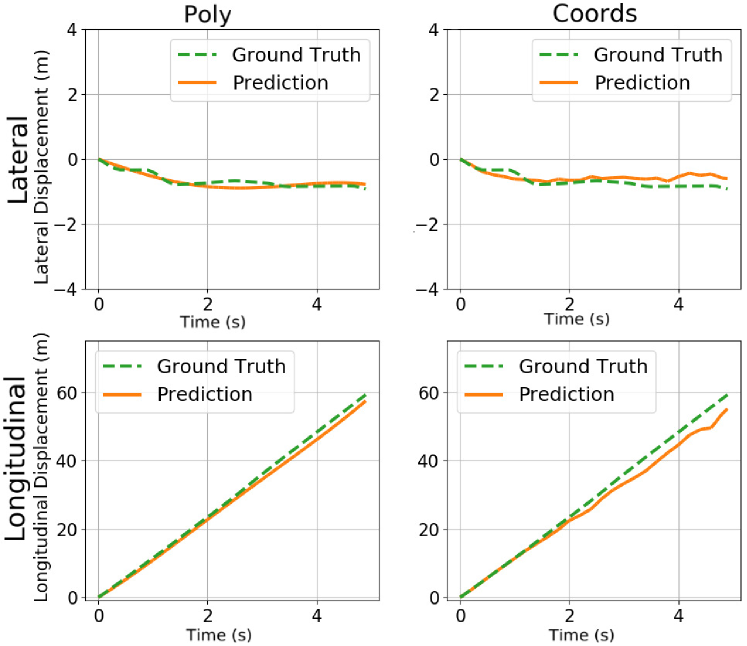
Fig. 1: Axis-wise visualisation of a random prediction from the test set. Right: coordinates prediction. Left: polynomial prediction. The top and bottom rows show the lateral and longitudinal axes, respectively. Notice how the polynomial prediction results in smoother and less jagged trajectories.

4.1 Visual Evaluation

Both prediction frameworks give visually appealing results. However, taking a closer look at a random example from the test set (Figure 1), the inconsistencies of the coordinates model are clearly visible. We explain this with two known properties of neural networks - over-fitting and prediction resolution.

During training, the network learns to over-fit its prediction offsets, subsequently harming its generalisation capacity. This is further discussed in subsection 4.3.

As noticed by works like [25], neural networks can reliably regress values, but only to a certain precision. The small regression inaccuracies which create the jagged trajectories make for a small portion of the total loss, making them hard to correct during training. By training our model on continuous trajectories, we are able to reach smoother, more natural looking results, as seen in Figure 1.

Offset (sec)	Coords baseline	Poly (ours)	CS-LSTM (M) [12]	MFP-1 [22]
1	0.43	0.55	0.62	0.54
2	1.00	0.93	1.27	1.16
3	1.72	1.64	2.09	1.90
4	2.76	2.64	3.10	2.78
5	3.98	3.85	4.37	3.83

Table 1: Results in RMSE of coordinates vs. polynomial training on NGSim [2]. For reference, two other SotA results are provided.

4.2 Quantifiable Evaluation

We further evaluate our framework on the common prediction horizon of five seconds. The results are presented in Table 1 along with two other works as a reference.

In a further experiment, we train both output types with both $5$ and $25$ anchor points. The results, shown in Figure 2 (right), are quite interesting. Looking at the $5$ anchors and the $25$ anchors models separately, one can see favourable performance of the polynomial models starting at around $1.5$ seconds. However, even between both types of models a clear improvement is visible, supporting our claim that models better generalise with the increased amount of anchors.

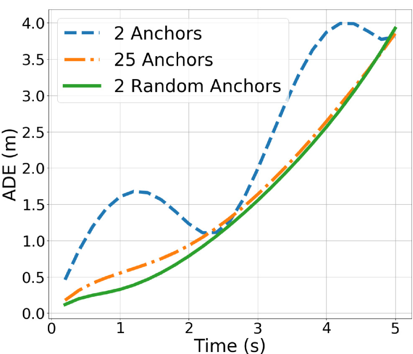
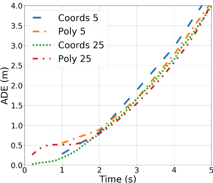
Fig. 2: Left: evaluating the random anchoring scheme. Even with as little as $2$ anchors the polynomial accuracies exceed the $25$ fixed anchors. Right: the results with $5$ and $25$ anchors per trajectory. For a given number of anchors, the polynomial prediction models outperform the classical coordinates.

4.3 Random Anchoring

We claim that when training on a fixed set of predetermined temporal offsets, the network only regards these few coordinates, thus learning less about the movement itself. As coordinates are fixed by definition, we test using our more flexible polynomials. The first model is trained using two anchors at $t_{25}$ and $t_{50}$ frames. The second model is trained on $25$ evenly spread frames, i.e. $[t_{2},t_{4},t_{6},\dots,t_{48},t_{50}]$. The third model is trained with two random anchors as described in Section 3.3.

The results are visualised in Figure 2 (left). Even with as little as two random labels per sample, the network manages to overcome the extreme over-fitting seen in the baseline and generalise better.

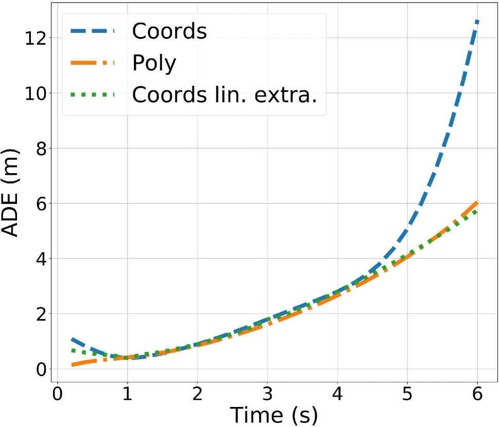
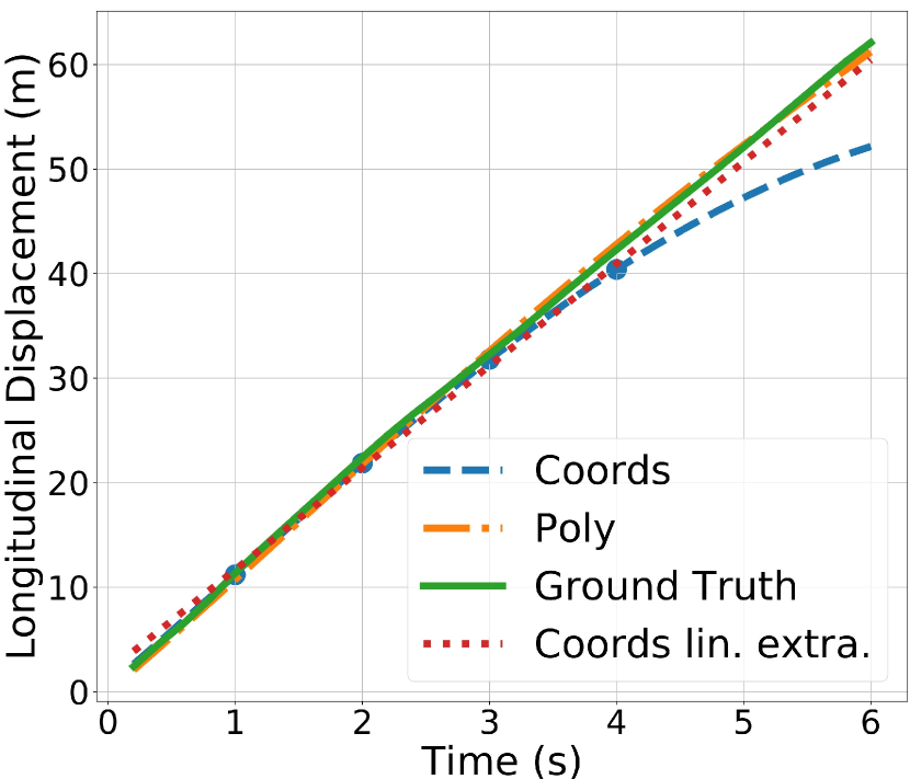
Fig. 3: Left: the ADE curve for the extrapolation experiment. Right: an example of an extrapolated longitudinal trajectory.

4.4 Extrapolation

To further test the generalisation capacities of our framework, we studied the extrapolation to unseen time steps.

A coordinates model and a polynomial one were trained on four seconds with four anchor points. We then evaluated them on a six seconds time span at five frames per second. For the coordinates extrapolation, we used NumPy’s polyfit function and fit both a linear curve and one of the same order as our polynomials.

The results averaging the entire test set are shown in Figure 3 (left). For the same polynomial degree our predictions better extend to new horizons. Yet the linear extrapolation of the coordinates prediction does similarly well. We use Figure 3 (right) as an example to explain this and show that often a simple linear interpolation performs well on average, especially on a dataset, which mostly includes straight trajectories.

5 Limitations

Despite the more accurate predictions, we have also noticed some limitations. For one, pedestrians typically require a higher degree of freedom than our polynomials currently enable. E.g., imagine a sequence of walking, stopping for a bit and then continuing to walk. Second, as seen in Figure 1, minor movements inside the lane are hard to represent. Yet such cruising artefacts are often irrelevant for most applications.

6 Conclusions

We presented a novel lightweight framework for predicting polynomial trajectories with artificial neural networks by adjusting only the output layer and the training scheme. With the rather general constraint of continuity our framework improves the generalisation of predicted trajectories. We are furthermore positive other fields, e.g., flight path planning, could also benefit from our development.

ACC

Adaptive Cruise Control

VAE

Variational Auto-Encoder

AEB

Autonomous Emergency Braking

RNN

Recurrent Neural Network

CNN

Convolutional Neural Network

ADE

Average Displacement Error

GRU

Gated Recurrent Units

GAN

Generative Adverserial Network

RMSE

Root Mean Squared Error

References

- [1] Kaiming He et al., “Mask R-CNN,” in Proceedings of the IEEE international conference on computer vision, 2017, pp. 2961–2969.
- [2] US Department of Transportation, “NGSIM next generation simulation,” 2006.
- [3] Robert Krajewski et al., “The HighD dataset: A drone dataset of naturalistic vehicle trajectories on german highways for validation of highly automated driving systems,” in 2018 21st International Conference on Intelligent Transportation Systems (ITSC), 2018, pp. 2118–2125.
- [4] Agrim Gupta et al., “Social GAN: Socially acceptable trajectories with generative adversarial networks,” in Proceedings of the IEEE Conference on Computer Vision and Pattern Recognition, 2018, pp. 2255–2264.
- [5] Namhoon Lee et al., “DESIRE: Distant future prediction in dynamic scenes with interacting agents,” in Proceedings of the IEEE Conference on Computer Vision and Pattern Recognition (CVPR), 2017.
- [6] Abduallah Mohamed et al., “Social-STGCNN: A social spatio-temporal graph convolutional neural network for human trajectory prediction,” in Proceedings of the IEEE/CVF Conference on Computer Vision and Pattern Recognition (CVPR), 2020.
- [7] Vineet Kosaraju et al., “Social-bigat: Multimodal trajectory forecasting using bicycle-gan and graph attention networks,” in Advances in Neural Information Processing Systems, 2019, pp. 137–146.
- [8] Dirk Helbing and Peter Molnar, “Social force model for pedestrian dynamics,” Physical review E, vol. 51, no. 5, pp. 4282, 1995.
- [9] Gianluca Antonini et al., “Discrete choice models of pedestrian walking behavior,” Transportation Research Part B: Methodological, vol. 40, no. 8, pp. 667–687, 2006.
- [10] C. G. Prevost et al., “Extended kalman filter for state estimation and trajectory prediction of a moving object detected by an unmanned aerial vehicle,” in 2007 American Control Conference, 2007, pp. 1805–1810.
- [11] A. Alahi et al., “Social LSTM: Human trajectory prediction in crowded spaces,” in IEEE Conf. on Computer Vision and Pattern Recognition, 2016.
- [12] Nachiket Deo and Mohan M Trivedi, “Convolutional social pooling for vehicle trajectory prediction,” in Proceedings of the IEEE Conference on Computer Vision and Pattern Recognition Workshops, 2018, pp. 1468–1476.
- [13] Mayank Bansal et al., “Chauffeurnet: Learning to drive by imitating the best and synthesizing the worst,” Robotics Science and Systems (RSS), 2019.
- [14] Mariusz Bojarski et al., “End to end learning for self-driving cars,” arXiv preprint arXiv:1604.07316, 2016.
- [15] Rajesh Rajamani, Vehicle dynamics and control, Springer Science & Business Media, 2011.
- [16] Henggang Cui et al., “Deep kinematic models for physically realistic prediction of vehicle trajectories,” arXiv preprint arXiv:1908.00219, 2019.
- [17] Charles Richter et al., “Polynomial trajectory planning for aggressive quadrotor flight in dense indoor environments,” in Robotics Research, pp. 649–666. Springer, 2016.
- [18] Alexandr Andoni et al., “Learning polynomials with neural networks,” in International conference on machine learning, 2014, pp. 1908–1916.
- [19] Juan-Manuel Pérez-Rúa et al., “Learning how to be robust: Deep polynomial regression,” arXiv preprint arXiv:1804.06504, 2018.
- [20] Grigorios G Chrysos et al., “P-nets: Deep polynomial neural networks,” in Proceedings of the IEEE/CVF Conference on Computer Vision and Pattern Recognition, 2020, pp. 7325–7335.
- [21] Alex Graves, “Generating sequences with recurrent neural networks,” CoRR, vol. abs/1308.0850, 2013.
- [22] Charlie Tang and Russ R Salakhutdinov, “Multiple futures prediction,” in Advances in Neural Information Processing Systems, 2019, pp. 15398–15408.
- [23] Junyoung Chung et al., “Empirical evaluation of gated recurrent neural networks on sequence modeling,” arXiv preprint arXiv:1412.3555, 2014.
- [24] Ashish Vaswani et al., “Attention is all you need,” in Advances in neural information processing systems, 2017, pp. 5998–6008.
- [25] J Bernardo et al., “Regression and classification using gaussian process priors,” Bayesian statistics, vol. 6, pp. 475, 1998.