Exactly solvable spin-$1/2$ XYZ models with highly-degenerate, partially ordered, ground states

Abstract

Exactly solvable models play a special role in Condensed Matter physics, serving as secure theoretical starting points for investigation of new phenomena. Changlani et al. [Phys. Rev. Lett. 120, 117202 (2018)] have discovered a limit of the XXZ model for $S=1/2$ spins on the kagome lattice, which is not only exactly solvable, but features a huge degeneracy of exact ground states corresponding to solutions of a three-coloring problem. This special point of the model was proposed as a parent for multiple phases in the wider phase diagram, including quantum spin liquids. Here, we show that the construction of Changlani et al. can be extended to more general forms of anisotropic exchange interaction, finding a line of parameter space in an XYZ model which maintains both the macroscopic degeneracy and the three-coloring structure of solutions. We show that the ground states along this line are partially ordered, in the sense that infinite-range correlations of some spin components coexist with a macroscopic number of undetermined degrees of freedom. We therefore propose the exactly solvable limit of the XYZ model on corner-sharing triangle-based lattices as a tractable starting point for discovery of quantum spin systems which mix ordered and spin liquid-like properties.

I Introduction

Calculations in condensed matter theory must generally bridge two different gaps. The first is the gap between model and experiment: any model simple enough to be successfully studied cannot capture every aspect of a real many body system, though we hope to capture the most important and interesting ones. The second is the gap between models and the actual calculation of physical quantities. Even when the model in question is simple to write down, it is usually necessary to employ some kind of approximation scheme during calculations.

Sometimes, however, the second gap is absent. There are models which are both physically relevant and for which exact calculations are possible. These have been important in the development of modern Condensed Matter physics, especially where they have been used to establish the theoretical possibility of novel phenomena or phases of matter. Notable examples of this include the Shastry-Sutherland model Shastry and Sutherland (1981), which established a featureless, gapped ground state in a many-body quantum spin model, and later found realization in SrCu₂(BO₃)₂ Miyahara and Ueda (1999); Kageyama et al. (1999) and the Kitaev honeycomb model Kitaev (2006), which a gave an example of a $Z_{2}$ quantum spin liquid with emergent Majorana fermions, and was later found to be relevant to various spin-orbit coupled magnets Jackeli and Khaliullin (2009); Banerjee et al. (2016, 2017); Kitagawa et al. (2018); Takagi et al. (2019).

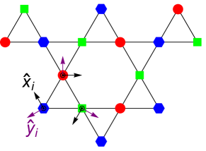
Figure 1: A three-color covering of the kagome lattice. Every triangle must include a site with each of three colors. The number of configurations satisfying this local rule grows exponentially with the system size. The exact ground states of the kagome XYZ model [Eq. (2)] map on to this three-coloring problem when the exchange parameters are chosen to obey Eq. (3). The coordinate axes $\hat{\bf x}_{i}$, $\hat{\bf y}_{i}$ indicate a choice of local basis for the spins, such that Eq. (2) is consistent with the symmetry of the kagome lattice, with the $\hat{\bf z}$ axis being uniformly perpendicular to the kagome plane. In contrast to the depicted coloring, this local spin basis is uniform across the lattice.

An interesting example of an exactly solvable spin-1/2 model has been pointed out by Changlani et al. Changlani et al. (2018). They considered the nearest neighbor XXZ model on the kagome lattice [Fig. 1]

$$\mathcal{H}_{\text{XXZ}}=\sum_{\langle ij\rangle}\left[J_{\perp}\left({S}^{x}_{i}{S}^{x}_{j}+{S}^{y}_{i}{S}^{y}_{j}\right)+J_{z}{S}^{z}_{i}{S}^{z}_{j}\right]\,,$$ (1)

and showed that at the special point $J_{z}/J_{\perp}=-1/2$ (denoted as the XXZ0 point Essafi et al. (2016)) the model has a set of exact, degenerate, ground states, the number of which grows exponentially with system size. These ground states can be written as simple product states, despite the fact that the Hamiltonian is composed of non-commuting terms and that general excited eigenstates are entangled. The ground states correspond with the solutions of the three-coloring problem on the kagome lattice Baxter (1970), in which the vertices of the lattice are colored with three different colors such that no triangle has two vertices of the same color [Fig. 1]. For a non-trivial, quantum many-body model to have such a huge degeneracy of ground states, with such a simple structure, is remarkable. The XXZ0 point is also significant in the wider phase diagram, being a point at which several different phases, including distinct quantum spin liquids, meet. It was suggested that the phase diagram of the model in the surrounding parameter space could be understood starting from this point Changlani et al. (2018, 2019).

Here we show how the XXZ0 point can be generalized to a wider set of exactly solvable anisotropic $S=1/2$ exchange models. Specifically, we consider the nearest-neighbor XYZ model on the kagome lattice:

$$\mathcal{H}_{\text{XYZ}}=\sum_{\langle ij\rangle}\left[J_{x}{S}^{x}_{i}{S}^{x}_{j}+J_{y}{S}^{y}_{i}{S}^{y}_{j}+J_{z}{S}^{z}_{i}{S}^{z}_{j}\right]\,,$$ (2)

i.e., the case where each component of the spin has a different associated exchange constant. If the basis for the spin operators $S^{\alpha}_{i}$ is defined with a local coordinate frame, as shown in Fig. 1, then this model is consistent with the symmetry of the lattice and can be considered as a limit of a more general model of anisotropic exchange Essafi et al. (2017), as shown in Appendix A.

We show that for any parameter set $\{J\}=(J_{x},J_{y},J_{z})$ fulfilling the conditions:

$$J_{x}+J_{y}+J_{z}>0\ \ \text{and}\ \ J_{x}J_{y}+J_{y}J_{z}+J_{z}J_{x}=0\,,$$ (3)

there exists a large manifold of exact product ground states, which generally differs from the solutions of the XXZ0 model, but retains the correspondence with the three-coloring problem.

We further show that despite having an extensive number of undetermined degrees of freedom, the ground states possess infinite range correlations of some spin components, coexisting with algebraic correlations. This is qualitatively reminiscent of the phenomenon of “magnetic moment fragmentation” Brooks-Bartlett et al. (2014); Rougemaille and Canals (2019); Lhotel et al. (2020) studied in both kagome Paddison et al. (2016); Canals et al. (2016); Dun et al. (2020) and pyrochlore Brooks-Bartlett et al. (2014); Petit et al. (2016); Benton (2016); Lefrancois et al. (2017) systems, but is particularly remarkable because it occurs in the exact ground states of a quantum model. This is in contrast to most known examples of moment fragmentation, which either occur in settings where the spins can be considered classical Brooks-Bartlett et al. (2014); Paddison et al. (2016); Canals et al. (2016); Lefrancois et al. (2017) or as a feature of the semi-classical dynamics rather than of the ground state Petit et al. (2016); Benton (2016).

The Article is structured as follows: Section II shows the construction of the family of exactly solvable models and their highly-degenerate ground states; Section III demonstrates the partial order of these ground states; Section IV demonstrates the presence of gapless excitations above these ground states despite the absence of continuous symmetry in the Hamiltonian; Section V discusses how our construction can be generalized to other lattices and spin lengths and gives a criterion for the presence of exact ground states of the type discussed here; lastly, Section VI contains a brief summary of our results and outlook for future work.

II Construction of exactly solvable Hamiltonian and its ground states

In this Section we show how to obtain the result that the ground states of Eq. (2) can be found exactly for all sets of parameters satisfying (3).

Any nearest-neighbor Hamiltonian on the kagome lattice can be written as a sum of single-triangle Hamiltonians:

$$\mathcal{H}_{\text{XYZ}}=\sum_{\triangle}\mathcal{H}_{\text{XYZ},\triangle}\,.$$ (4)

The spectrum of the single triangle Hamiltonian $\mathcal{H}_{\text{XYZ},\triangle}$ is composed of a quadruplet with energy

$$e_{q}=-\frac{1}{4}(J_{x}+J_{y}+J_{z})\,,$$ (5)

and of two doublets with energies

$$e_{d\pm}=-e_{q}\pm 2\sqrt{e_{q}^{2}-\frac{3}{16}\Lambda}\,\,,$$ (6)

where $\Lambda=J_{x}J_{y}+J_{y}J_{z}+J_{z}J_{x}\,.$ When $\Lambda=0$ and $e_{q}<0$ (cf. Eq. (3)), the spectrum is composed of a 6-fold degenerate ground state $e_{q}=e_{d-}=e_{0}$, and of an excited doublet $e_{d+}$.

In this case it follows that the Hamiltonian can be written as a sum of non-commuting projectors:

$$\mathcal{H}_{\text{XYZ},\Lambda=0}=\sum_{\triangle}[(e_{d+}-e_{0})P_{\triangle}+e_{0}]\,,$$ (7)

with $P_{\triangle}$ being the operator that projects onto the pair of single-triangle excited states:

$$P_{\triangle} =\lvert d+,+\rangle\langle d+,+\rvert\ \ +\ \ \lvert d+,-\rangle\langle d+,-\rvert\,,$$ (8)

$$\lvert d+,+\rangle =\cos(\alpha)\frac{\lvert\uparrow\uparrow\downarrow\rangle+\lvert\uparrow\downarrow\uparrow\rangle+\lvert\downarrow\uparrow\uparrow\rangle}{\sqrt{3}}+\sin(\alpha)\lvert\downarrow\downarrow\downarrow\rangle\,,$$

$$\lvert d+,-\rangle =\cos(\alpha)\frac{\lvert\downarrow\downarrow\uparrow\rangle+\lvert\downarrow\uparrow\downarrow\rangle+\lvert\uparrow\downarrow\downarrow\rangle}{\sqrt{3}}+\sin(\alpha)\lvert\uparrow\uparrow\uparrow\rangle\,,$$

$$\tan(\alpha) =\frac{(J_{x}-J_{y})}{\sqrt{3}(J_{x}+J_{y})}\,.$$

Since $e_{d+}>e_{0}$, the coefficient in front of the projection operator in Eq. (7) is positive and any state which is annihilated by all of the $P_{\triangle}$ is a ground state.

We can search for states annihilated by $P_{\triangle}$ amongst the set of site-product states:

$$\lvert\Psi(\{\theta\},\{\phi\})\rangle=\prod_{{\rm sites}\ j}\bigg{(} \cos\left(\tfrac{1}{2}\theta_{j}\right)e^{-i\tfrac{1}{2}\phi_{j}}\lvert\uparrow_{j}\rangle$$ (9)

$$~{}~{}+\sin\left(\tfrac{1}{2}\theta_{j}\right)e^{i\tfrac{1}{2}\phi_{j}}\lvert\downarrow_{j}\rangle\bigg{)}\,.$$

As we show below, there are many product states on the lattice which are annihilated by $P_{\triangle}$. Our strategy is to first identify these product states on a single triangle (Section II.1) and then generate ground states on the lattice by tiling single triangle ground states across the system.

II.1 Product ground states on a single triangle

For a single triangle, the possible product wave functions [Eq. (9)] are parametrized by $6$ variables: the $\theta_{j}$ and $\phi_{j}$ of each of the three sites. To be ground states, these wavefunctions need to satisfy four constraints: the real and imaginary parts of their overlaps with $\lvert d+,\pm\rangle$ [Eq. (8)] must vanish. This suggests a $6-4=2$ dimensional surface of exact product state ground states for a single triangle. We have verified that such a surface, that we shall call $\mathcal{M}$, indeed exists for all $\{J\}$ obeying (3). An exact parameterization of $\mathcal{M}$ has also been found, but its derivation is quite involved and is therefore presented in Appendix B.

Nonetheless, the solutions for two limits of (3) are easily found, and the general case can be understood as an interpolation between these two limits [Fig. 2]. The first limit is the XXZ0 limit Changlani et al. (2018) $J_{x}=J_{y}=2/3$, $J_{z}=-1/3$ in which case $\mathcal{M}$ is composed of two spheres:

$$\theta_{1} =\theta_{2}=\theta_{3}\,,$$

$$\phi_{1} =\phi_{2}\pm\frac{2\pi}{3}=\phi_{3}\mp\frac{2\pi}{3}\,.$$ (10)

These two spheres meet at the points $\theta_{1}=0$ and $\pi$ corresponding to the all-up and all-down states, as illustrated under Fig. 2 a).

The other easily solved limit is the Ising limit: $J_{x}=J_{y}=0$, $J_{z}=1$. In this case, product ground states have $\theta=0$ (spin fully up) on one site and $\theta=\pi$ (spin fully down) on another, with $\theta,\phi$ on the remaining site completely free. The product ground state manifold $\mathcal{M}$ is thus composed of six spheres, each connected to two other spheres at the points where two spins have $\theta=0$ or $\theta=\pi$. This is illustrated in Fig. 2 b). The six spheres correspond to the six ways of assigning an up spin, a down spin, and a free spin to the three sites of a triangle. The surface of each individual sphere corresponds to the direction of the expectation value of the free spin.

The manifold for more general exactly solvable $\{J\}$ interpolates between these two limits by smoothing out the singular points where the spheres meet so as to produce a manifold with the topology of a torus. This interpolation can be made precise by parameterizing the $\{J\}$ satisfying (3) as $J_{x/y}=1/3-(2/3)\cos(\kappa\pm 2\pi/3)$, $J_{z}=1/3-(2/3)\cos(\kappa)$. Then $\kappa=0$ is a XXZ0 point [Fig. 2 a)], $\kappa=\pi/3$ an Ising point [Fig. 2 b)], and the $\mathcal{M}$ for generic $\kappa\in\langle 0,\pi/3\rangle$ smoothly deforms as we vary $\kappa$ from one limiting case to the other [Fig. 2 c)]. In between, $\mathcal{M}$ has the topology of a torus, and this torus pinches at two (six) points as $\kappa\to 0$ ($\kappa\to\pi/3$).

We have checked numerically that the surface of single triangle solutions for general parameters has genus $g=1$ (see Appendix C and Supplemental Material sup ). This is itself an unusual situation, which can be contrasted (e.g.) with the exact ground states of a Heisenberg ferromagnet which cover the surface of a sphere.

Having obtained the exact solutions on a single triangle, the question is then how much freedom there is to tile these solutions over the whole lattice.

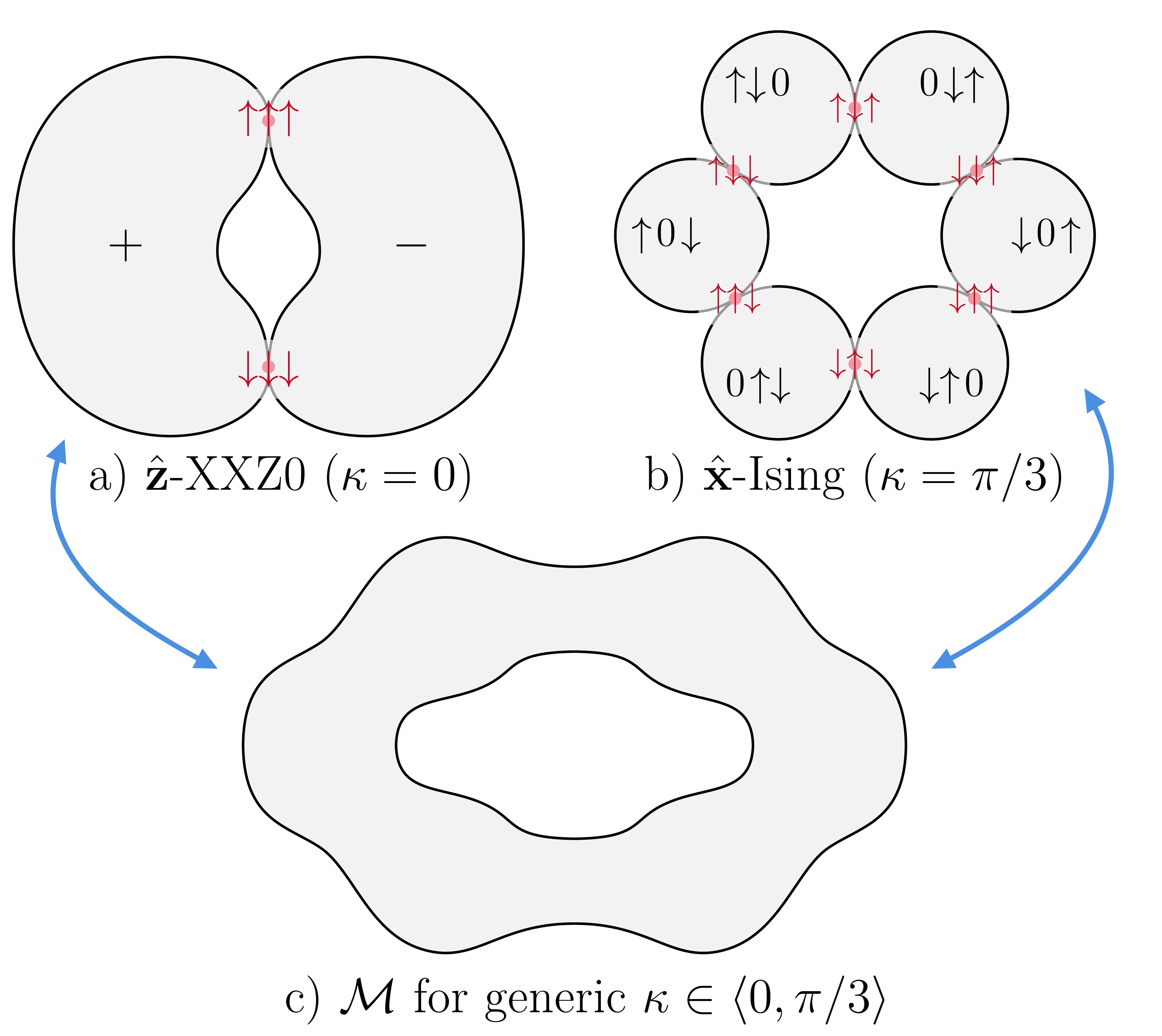
Figure 2: Schematic representation of the topology of the product ground state manifold of a triangle $\mathcal{M}$ for: a) the $\hat{\bf z}$-XXZ0 point ($\kappa=0$, $J_{x}=J_{y}=2/3$, $J_{z}=-1/3$), b) the $\hat{\bf x}$-Ising point ($\kappa=\pi/3$, $J_{x}=1$, $J_{y}=J_{z}=0$), and c) generic $\kappa\in\langle 0,\pi/3\rangle$ between these two limits. The $\mathcal{M}$ of the XXZ0 point is made of two spheres with different chiralities, denoted $+$ and $-$, that touch at their poles. The points of contact are marked with red dots, and the respective spin configurations are written on top of these contact points. The Ising point $\mathcal{M}$ is made of six spheres that have one $\uparrow$ spin, one $\downarrow$ spin, and one free spin, which we denoted with a $0$. These six spheres touch adjacent spheres at the specified red points. In between, $\mathcal{M}$ has the topology of a torus. Although drawn here as (deformed) circles, lines, etc., all of the above sketches should be understood as representing 2D surfaces embedded in the 6D space of all possible $\theta_{j},\phi_{j}$ in a triangle.

II.2 Exact ground states on the lattice

Any $S=1/2$ product state [Eq. (9)] can be labelled by the expectation values of the spin operators $\langle{\bf S}_{i}\rangle=(\langle S^{x}_{i}\rangle,\langle S^{y}_{i}\rangle,\langle S^{z}_{i}\rangle)$, up to a global phase. Let us fix $\langle{\bf S}_{i}\rangle$ on one particular site and then seek to build a solution on the lattice from there.

It turns out we can choose any direction for the first $\langle{\bf S}_{i}\rangle$ and still find configurations for the surrounding spins such that the triangle and system are in a ground state. Specifying the first $\langle{\bf S}_{i}\rangle$ will in general remove the continuous freedom identified for the single triangle in II.1, leaving only a discrete set of possibilities for the neighboring spins to remain in the ground state.

If we fix $\langle{\bf S}_{i}\rangle$ to ${\bf S}_{0}$ and consider one of the two triangles connected to the site $i$, then the remaining spins $j,k$ on that triangle can take only one of two configurations. These two configurations are related to one another by a permutation symmetry that swaps the remaining pair of sites,

$$\langle{\bf S}_{j}\rangle={\bf S}_{1}\,,\langle{\bf S}_{k}\rangle={\bf S}_{2}\ \ \text{or}\ \ \langle{\bf S}_{j}\rangle={\bf S}_{2}\,,\langle{\bf S}_{k}\rangle={\bf S}_{1}\,,$$ (11)

with the values ${\bf S}_{1}$ and ${\bf S}_{2}$ being fixed by ${\bf S}_{0}$.

Propagating this throughout the system, consistency between triangles will force all sites to take one of the three expectation values $({\bf S}_{0},{\bf S}_{1},{\bf S}_{2})$. Some examples of allowed triads of expectation values $({\bf S}_{0},{\bf S}_{1},{\bf S}_{2})$ for $J_{x}/J_{z}=1/4$, $J_{y}/J_{z}=-1/5$ are shown in Fig. 3. Provided that the first triangle $ijk$ was in a ground state, the permutation symmetry of $\mathcal{H}_{\text{XYZ}}$ guarantees that any triangle where each of the three expectation values is represented once is also a ground state.

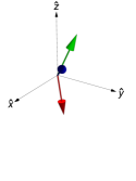
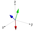
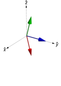
Figure 3: Examples of allowed triads of spin expectation values which may occur together on a triangle, for an example parameter set $J_{x}/J_{z}=1/4$, $J_{y}/J_{z}=-1/5$. Different possible product ground state wavefunctions correspond to a different choice of one such triad on the first triangle, and then a tiling of the lattice with the three members of the triad, with each member occurring once on each triangle. Animations of all allowed spin triads for various parameter sets $\{J\}$ are included in the Supplementary Material sup .

Provided that $({\bf S}_{0},{\bf S}_{1},{\bf S}_{2})$ are all distinct from one another (which is true for generic members of the ground state manifold), these conditions are in precise correspondence to the rules of the three coloring model. Thus, the set of product state solutions to $\mathcal{H}_{\text{XYZ},\Lambda=0}$ is given by the space of three-color configurations, along with two continuous degrees of freedom which were used up by fixing the first spin.

This establishes our main result: that $\mathcal{H}_{\text{XYZ}}$ with parameters chosen to obey Eq. (3) has a set of exact, product, ground states, the number of which grows exponentially with system size. The wavefunctions described by Eq. (9) are not all linearly independent, so the actual ground state degeneracy is not the same as the number of product state solutions. Nevertheless, if the number of product state solutions grows exponentially with system size, it should be expected that the number which are linearly independent also grows exponentially. This was verified for the case of the XXZ0 model in Ref. Changlani et al., 2018.

We have checked using exact diagonalization on small clusters that there is indeed a collapse of many excited states towards the ground state approaching the points in parameter space given by (3), consistent with the establishment of a macroscopic ground state degeneracy in the thermodynamic limit. This is shown for a 24-site cluster in Fig. 4.

It is possible that there are also additional ground states, beyond the product ground states found here. Changlani et al. found numerically that there are indeed some additional ground states in the XXZ0 limit for lattices with periodic boundaries, although not with open boundaries Changlani et al. (2018).

The set of exactly solvable XYZ models described by (3) includes both the XXZ0 model ($\{J\}\propto(\frac{2}{3},\frac{2}{3},\frac{-1}{3})$ and permutations) and the Ising model ($\{J\}\propto(0,0,1)$ and permutations), three times each. The Ising model represents a singular limit for the set of product ground states because if two spins on a triangle are fixed to be one up and one down, the third spin is actually completely undetermined, increasing the freedom in the construction of ground states on the lattice.

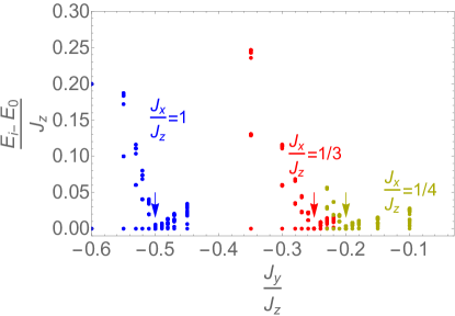
Figure 4: Low energy spectra of the XYZ model Eq. (2) from exact diagonalization of a 24-site cluster, as a function of $J_{y}/J_{z}$ for $J_{x}/J_{z}=1$, $1/3$, $1/4$. A collapse of the excited states towards zero energy can be seen approaching the points where Eq. (3) is satisfied (respectively at $J_{y}/J_{z}=-1/2$, $-1/4$, $-1/5$ for the three chosen values of $J_{x}/J_{z}$, as indicated by arrows).

III Partial Ordering in the Ground States

In this Section we argue that the exact ground states identified in Section II possess infinite range correlations, coexisting with the algebraic correlations implied by the three-color mapping and are in this sense partially ordered.

The allowed ground state configurations of spin expectation values on a single triangle generally have a finite value of ${\bf m}=\langle{\bf S}_{0}\rangle+\langle{\bf S}_{1}\rangle+\langle{\bf S}_{2}\rangle$. This is illustrated in Fig. 5, where the minimum and maximum value of $|{\bf m}|$ over the possible single triangle ground states is plotted as a function of $J_{y}/J_{z}$. Note that ${\bf m}$ would not be the same as the magnetisation in a real system, because of the local basis used to define the spins [Fig. 1].

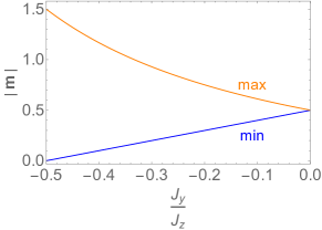
Figure 5: Maximum and minimum possible ground state values of $|{\bf m}|=|\langle{\bf S}_{0}\rangle+\langle{\bf S}_{1}\rangle+\langle{\bf S}_{2}\rangle|$ within the set of exact product ground states on a single triangle as a function of $J_{y}/J_{z}$, for sets of parameters obeying condition (3). Apart from at the XXZ0 point ($J_{y}/J_{z}=-1/2$), all allowed product ground states have a finite ${\bf m}$. Once ${\bf m}$ is fixed on the first triangle it will be the same on all triangles throughout the lattice, apart from in the Ising limit, ($J_{y}/J_{z}=0$) where some individual spins can be rotated freely. This establishes that, for general parameter sets obeying (3), the ground states carry infinite range spin correlations, coexisting with the algebraic correlations implied by the three-color mapping.

Since the remaining triangles in the lattice must only feature permutations of the spin expectation values on the first triangle (see Section II.2), and since ${\bf m}$ is invariant under those permutations, we conclude that all triangles must have the same value of ${\bf m}$. This implies that ${\bf M}=\sum_{\triangle}{\bf m}_{\triangle}$ has a macroscopic value in any given product state and that there are infinite range correlations of the spin component parallel to ${\bf m}$. These infinite-range correlations must coexist with the algebraic correlations that are also present due to the mapping between the spin configurations and the three-color model.

IV Gapless Excitations

In addition to the many ground states, this exactly solvable model also possesses gapless excitations.

We demonstrate this below by making use of the continuous degeneracy of the ground states identified in Section II.1, and a trial wave function for the excitations based on the single mode approximation. Starting from a translationally invariant member of the set of ground states one can construct excitations using the generators of rotations within the single triangle ground state manifold, and show that these are gapless in the long wavelength limit.

Let us emphasize that the considerations of this section depend only on the continuous degeneracy of the ground states, and not on the discrete degeneracy of how one can tile the one triangle solution across the whole lattice. Thus the argument of this section would work equally well for (e.g.) exactly solvable XYZ models on the triangular lattice, which would retain the continuous degeneracy of the kagome case considered here, but for which only 6 consistent three-colorings are possible.

The gapless excitations are similar to Nambu-Goldstone modes, except that unlike ordinary Nambu-Goldstone modes the associated symmetry generator $\mathcal{G}$ does not commute with the Hamiltonian

$$[\mathcal{H}_{\text{XYZ}},\mathcal{G}]\neq 0\,,$$ (12)

but rather the commutator annihilates a ground state:

$$[\mathcal{H}_{\text{XYZ}},\mathcal{G}]\lvert\Psi_{0}\rangle=0\,.$$ (13)

One way of motivating the above is to consider a one-parameter family of ground states $\lvert\Psi_{t}\rangle$ that we know exists because of the continuous degeneracy. Then it is always possible to find an unitary operator $\mathcal{U}_{t}$ that maps $\lvert\Psi_{0}\rangle\mapsto\lvert\Psi_{t}\rangle$. We may then identify the quasisymmetry generator with $\mathcal{G}=i\partial_{t}\mathcal{U}_{t}|_{t=0}$. Since $E_{0}\lvert\Psi_{1}\rangle=\mathcal{H}_{\text{XYZ}}\mathcal{U}_{t}\lvert\Psi_{0}\rangle=\mathcal{U}_{t}\mathcal{H}_{\text{XYZ}}\lvert\Psi_{0}\rangle$, (13) follows. Qualitatively, we may say that $\mathcal{G}$ becomes an exact symmetry only in the zero-energy limit.

Of course, it may be the case that some of the ground state quasi-symmetry generators are also genuine symmetry generators. The XXZ0 point, considered in Section II.1, is a good example. From (10) it is evident that a global rotation around the $\hat{\bf z}$ axis maps a ground state to a ground state. In fact, this is an exact symmetry of the XXZ Hamiltonian. On the other hand, rotating the spins by $\theta_{i}\mapsto\theta_{i}+\delta\theta$ also maps a ground state to a ground state, but is not a genuine symmetry. Note how in the case of the $\theta_{i}\mapsto\theta_{i}+\delta\theta$ transformation, the generator $\mathcal{G}$ depends on the starting ground state $\lvert\Psi_{0}\rangle$.

To begin with, we choose a member of the set of product ground states to construct excitations around. In such a ground state, each spin expectation value takes one of three values $\langle{\bf S}_{r}\rangle$, $\langle{\bf S}_{g}\rangle$, and $\langle{\bf S}_{b}\rangle$, according to whether the site is red, green, or blue in the three-color representation of the state. $\lvert\Psi_{0}\rangle$ is chosen to be the state corresponding to a translationally invariant three-coloring of the lattice. Later we comment on more general red-green-blue patterns.

The existence of a continuous two-dimensional manifold of exact product ground states on the single triangle implies the existence of infinitesimal global rotations which keep every triangle, and therefore the system as a whole, in a ground state.

There are two independent generators of these rotations for every starting ground state (spin triad). We will pick one of them, which we label $\mathcal{G}=\sum_{i}g_{i}$. The site generator $g_{i}$ depends on the color of site $i$ in the three-color tiling of the ground state.

We now do a site-dependent coordinate transformation on the spin basis $\{x,y,z\}\to\{u_{i},v_{i},w_{i}\}$, with the new coordinate axes chosen such that ${\bf\hat{w}}_{i}$ aligns with the expectation value of spin $i$ in the ground state and so that the generators $g_{i}$ are proportional to rotations around ${\bf\hat{u}}_{i}$. The spin operators in this basis then satisfy:

$$S^{w}_{i}\lvert\Psi_{0}\rangle =\frac{1}{2}\lvert\Psi_{0}\rangle\,,\quad\forall\,i\,,$$ (14)

$$g_{i} =U_{i}\,S^{u}_{i}\,,$$ (15)

where $U_{i}$ is a real scaling factor that depends only on the coloring of the site $i$. (In general, $U_{i}$ also depend on the three spin vectors $\langle{\bf S}_{r}\rangle$, $\langle{\bf S}_{g}\rangle$, and $\langle{\bf S}_{b}\rangle$, but these are the same across $\lvert\Psi_{0}\rangle$.) It is normalized according to

$$\sum_{c=r,g,b}(U_{c})^{2}=1\,.$$ (16)

Since the local ${\bf\hat{u}}_{i}$ axes have been chosen to correspond with the rotation axes that keep the system in a ground state, it must be true that:

$$\sum_{i}[\mathcal{H}_{\text{XYZ}},U_{i}S^{u}_{i}]\lvert\Psi_{0}\rangle=0\,.$$ (17)

We then consider the following variational wavefunction for the excitations, based on the single mode approximation,

$$\lvert{\rm ex},{\bf q}\rangle =\mathcal{G}({\bf q})\lvert\Psi_{0}\rangle\,,$$ (18)

$$\mathcal{G}({\bf q}) =\frac{1}{\sqrt{N}}\sum_{i}U_{i}S^{u}_{i}\exp(i{\bf q}\cdot{\bf r}_{i})\,,$$ (19)

where $N$ is the number of unit cells. The wavefunction $\lvert{\rm ex},{\bf q}\rangle$ describes a spin wave-like excitation.

$\lvert{\rm ex},{\bf q}\rangle$ is orthogonal to $\lvert\Psi_{0}\rangle$ because $\langle\Psi_{0}|S^{u}_{i}|\Psi_{0}\rangle$ vanishes everywhere. At finite ${\bf q}$ and in the thermodynamic limit $N\to\infty$, it is also orthogonal to the other members of the ground state manifold. Because of this, the expectation value of the energy in $\lvert{\rm ex},{\bf q}\rangle$ is an upper bound on the energy of excitations with momentum ${\bf q}$:

$$E(\mathbf{q})-E_{0}\leq\frac{\langle\Psi_{0}|\mathcal{G}(-{\bf q})[\mathcal{H}_{\text{XYZ}},\mathcal{G}({\bf q})]|\Psi_{0}\rangle}{\langle\Psi_{0}|\mathcal{G}(-{\bf q})\mathcal{G}({\bf q})|\Psi_{0}\rangle}\,.$$ (20)

The denominator $\langle\Psi_{0}|\mathcal{G}(-{\bf q})\mathcal{G}({\bf q})|\Psi_{0}\rangle=\frac{1}{4}$, and we can set $E_{0}=0$ (i.e., measure all energies relative to the ground state), so that

$$E(\mathbf{q})\leq 4\langle\Psi_{0}|\mathcal{G}(-{\bf q})[\mathcal{H}_{\text{XYZ}},\mathcal{G}({\bf q})]|\Psi_{0}\rangle\,.$$ (21)

Due to Eq. (17), the ${\bf q}\to{\bf 0}$ limit of Eq. (21) vanishes:

$$\lim_{{\bf q}\to{\bf 0}}E(\mathbf{q})=0\,,$$ (22)

implying gapless excitations.

The part of Eq. (21) which is linear in ${\bf q}$ also vanishes:

$$\frac{1}{N}\sum_{m,n}i{\bf q}\cdot{\bf r}_{m}\langle\Psi_{0}|[U_{n}S^{u}_{n},\mathcal{H}_{\text{XYZ}}]U_{m}S^{u}_{m}|\Psi_{0}\rangle$$

$$-\frac{1}{N}\sum_{m,n}i{\bf q}\cdot{\bf r}_{n}\langle\Psi_{0}|U_{n}S^{u}_{n}[\mathcal{H}_{\text{XYZ}},U_{m}S^{u}_{m}]|\Psi_{0}\rangle=0\,,$$ (23)

which also follows from Eq. (17).

This leads us to the conclusion that the dispersion of excitations has a quadratic upper-bound at small $q$:

$$E({\bf q})\leq\zeta\,q^{2}\,.$$ (24)

This also agrees with a linear spin wave analysis which finds quadratically dispersing excitations around the translationally invariant exact ground states.

Although not obvious, a detailed analysis of the properties of the coupling matrix $J_{ij}$ in the new basis $\{u_{i},v_{i},w_{i}\}$ shows that the second generator of symmetry has $g_{i}^{\prime}=U_{i}S^{v}_{i}$ with the same scaling factors $U_{i}$ from Eq. (15). Thus one finds that the commutator $[\mathcal{G},\mathcal{G}^{\prime}]$ has a non-vanishing expectation value in the ground state $|\Psi_{0}\rangle$, implying that the two generators represent only one degree of freedom (cf. $[x,p]=i\hbar$) Watanabe (2020). In the spin wave analysis this is reflected in the fact that there is only one gapless mode, despite the two broken quasi-symmetry generators.

For more general coloring patterns (that are not translationally symmetric), $\mathcal{G}({\bf q})$ may still be used to probe the low-lying excitations, but this time ${\bf q}$ cannot be identified with the momentum. The above argument thus suggests that low-lying excitations still exist even for more general RGB patterns.

With that said, one should keep in mind that the above argument may fail if the upper bound from (20) is discontinuous at ${\bf q}={\bf 0}$, (see e.g. Supplementary Material of [Matsuyama and Greensite, 2019]).

To verify that our upper bound is continuous, we evaluate it by noting that only averages of the form $\langle\Psi_{0}|S_{i}^{u}S_{i}^{\mu}S_{i+\delta}^{w}|\Psi_{0}\rangle$ for $\mu=u,v$ are non-vanishing, giving:

$$\langle\Psi_{0}|\mathcal{G}(-{\bf q})[\mathcal{H}_{\text{XYZ}},\mathcal{G}({\bf q})]|\Psi_{0}\rangle=$$

$$-\frac{1}{8N}\sum_{i\delta}(U_{i})^{2}J^{i,i+\delta}_{ww}+\frac{1}{8N}\sum_{i\delta}U_{i}U_{i+\delta}e^{i{\bf q}\cdot{\bf\delta}}(J^{i,i+\delta}_{vv}-iJ^{i,i+\delta}_{uv})\,.$$

(25)

From the fact that $|\Psi_{0}\rangle$ is an exact eigenstate, it follows that in the new basis the exchange coefficients satisfy $J^{ij}_{uu}=J^{ij}_{vv}=J^{ij}_{\perp}$ and $J^{ij}_{uv}=-J^{ij}_{vu}=d^{ij}$. The exchange coefficients $J^{ij}_{\mu\nu}$ also depend only on the coloring of the sites $i$ and $j$ and satisfy $J^{ij}_{\mu\nu}=J^{ji}_{\nu\mu}$. Moreover, from the fact that the change in energy within one triangle is to second order equal to zero when we vary the spins with $\mathcal{G}$, it follows that:

$$2J_{\perp}^{rg}U_{r}U_{g}+2J_{\perp}^{gb}U_{g}U_{b}+2J_{\perp}^{br}U_{b}U_{r}-(J_{ww}^{rg}+J_{ww}^{rb})(U_{r})^{2}$$

$$-(J_{ww}^{gr}+J_{ww}^{gb})(U_{g})^{2}-(J_{ww}^{br}+J_{ww}^{bg})(U_{b})^{2}=0\,.$$ (26)

Applying to Eq. (25), we obtain:

$$\frac{\langle\Psi_{0}|\mathcal{G}(-{\bf q})[\mathcal{H}_{\text{XYZ}},\mathcal{G}({\bf q})]|\Psi_{0}\rangle}{\langle\Psi_{0}|\mathcal{G}(-{\bf q})\mathcal{G}({\bf q})|\Psi_{0}\rangle}=$$

$$\frac{1}{4N}\sum_{\langle ij\rangle}U_{i}U_{j}\left[J^{ij}_{\perp}[\cos\left({\bf q}\cdot({\bf r}_{j}-{\bf r}_{i})\right)-1]+d^{ij}\sin\left({\bf q}\cdot({\bf r}_{j}-{\bf r}_{i})\right)\right],$$

which is indeed continuous and vanishing in the limit ${\bf q}\to{\bf 0}$.

We therefore conclude that the partially ordered exact ground states of the XYZ model have gapless excitations, despite the absence of continuous symmetry in the original Hamiltonian.

V Recipe for constructing further exactly solvable models

Our work exposes a simple recipe for the construction of further highly degenerate exactly solvable models, of the same kind as those discussed here.

First, one must define a Hamiltonian for quantum spins of length $S$ on a set of corner sharing units (for instance, triangles or tetrahedra), with the Hamiltonian on each unit being symmetric under permutations of the sites. Then one must tune the parameters such that the degeneracy $d_{0}$ of the ground state of the single unit Hamiltonian is large enough that product wavefunctions on the single unit have enough free parameters to be made orthogonal to all of the excited states.

If $n$ is the number of sites in each unit then, the total number of states in the single unit spectrum is $(2S+1)^{n}$ and a single unit product state has $4Sn$ degrees of freedom. Requiring that the real and imaginary parts of the overlap with every excited state in the single unit spectrum vanishes gives $2((2S+1)^{n}-d_{0})$ constraints, so to be able to find product-like solutions we need:

$$d_{0}\geq(2S+1)^{n}-2Sn\,.$$ (28)

If the single unit Hamiltonian can be tuned to have a sufficiently large $d_{0}$ then one can search for product-like ground states. If, in these ground states, all $n$ sites in the unit are distinguishable from one another (e.g., if the spin expectation values differ on the sites), and the single-unit Hamiltonian has a permutation symmetry under the swapping of sites, then the problem of tiling solutions over the whole lattice becomes an $n$-coloring problem. We anticipate that this recipe can be used to construct further exactly solvable models on other lattices.

In the case of $S=1/2$ spins on the kagome lattice, the minimal $d_{0}$ is $5$ (cf. $d_{0}=6$ for the models considered in this manuscript). In a model with $d_{0}=5$, there would be no continuous degrees of freedom left in the ground state, but only discrete degrees of freedom from the three-coloring pattern.

The exactly solvable “two-coloring” models identified in Ref. Pal et al., can also be seen as an example of the construction described above, with the corner-sharing units being single bonds ($n=2$) and the requirement for exact solvability $d_{0}\geq 2$. The “two-coloring” models in Ref. Pal et al., have $d_{0}=3$.

VI Summary and outlook

We have demonstrated that the exactly solvable model pointed out in Ref. Changlani et al., 2018 is a member of a wider family of exactly solvable models, and that the ground states of these models possess coexisting infinite-range and algebraic correlations. The combination of the large ground state degeneracy, and the coexistence of infinite-range and algebraic correlations suggest an analogy with the phenomenon of “magnetic moment fragmentation” Brooks-Bartlett et al. (2014); Rougemaille and Canals (2019); Lhotel et al. (2020); Paddison et al. (2016); Canals et al. (2016); Petit et al. (2016); Benton (2016); Lefrancois et al. (2017) but the case here is distinguished by the fact that it occurs in the exact ground states of a quantum model.

Our conclusions generalize straightforwardly to XYZ models on other triangle-based lattices, such as the hyperkagome lattice.

The models described here, fall into a wider category of frustrated systems possessing a large number of low energy states, defined by local constraints. In such cases, a description of the low energy physics in terms of emergent gauge fields and charges is frequently useful Isakov et al. (2004); Moessner and Sondhi (2010); Cépas and Ralko (2011), and this may be an interesting avenue to investigate further for the present case.

The exact ground states we have defined are not themselves quantum spin liquids, since they lack quantum entanglement and have a large non-topological degeneracy. Nevertheless, highly degenerate points of a model are often a good starting point for discovery of spin liquids because small perturbations can stabilize a variety of non-trivial superpositions of the degenerate states. In this case, given the partial ordering of the ground states, perturbing the models identified here may be a way to stabilize phases which combine the interesting features of a quantum spin liquid (entanglement, fractional excitations) with spontaneous symmetry breaking. With this in mind, we suggest that a numerical study of the ground states of $\mathcal{H}_{\text{XYZ}}$ for parameter sets close to the exactly solvable limit may be a rewarding subject for future work.

In view of the large number of ground states, and low lying excited states, the physics of the exactly solvable models at finite temperature is also an interesting topic for the future. In particular, it is possible that at $T>0$ thermal order-by-disorder will lead to a breaking of the ground state degeneracy. Quantum ($T=0$) order-by-disorder is conclusively ruled out for the models described in this work, because the exact ground states and their energies are known. It may nevertheless be the case that thermal fluctuations can distinguish between the states, leading to an entropic selection at finite temperature. The low energy gapless modes discussed in Section IV are likely to play a key role in this selection, if it occurs.

A further unusual feature of the XYZ model presented here is that even the solutions to the single triangle problem are topologically non-trivial, in that the continuous manifold of single-triangle solutions has the topology of a torus. Whether interesting phenomena can be derived from this by, for example, adiabatically moving the system around this manifold is something which remains to be seen.

Finally we note that these exact ground states may also be of interest from the point of view of non-equilibrium physics. With a simple alteration of the Hamiltonian Lee et al. (2020) the exact ground states can be turned into many-body quantum scars: highly excited states which violate the eigenstate thermalization hypothesis. The XYZ models proposed here offer a chance to explore this in a setting which lacks continuous spin rotation symmetry.

Appendix A Relationship between XYZ model and more general anisotropic exchange models on the kagome lattice

Here we elaborate on the relationship between the XYZ model studied in the main text and the model dicussed in Ref. Essafi et al., 2017. The model discussed in Ref. Essafi et al., 2017 gives the most general set of nearest neighbour interactions consistent with the symmetries of the lattice, including a mirror symmetry in the kagome plane itself. In total, the symmetries considered comprise the inversion and translation symmetries of the kagome lattice along with the three point group symmetries shown in Fig. 6.

The Hamiltonian of this model is:

$$\mathcal{H}_{\sf gen}=\sum_{\langle ij\rangle}S^{\alpha}_{i}J^{\alpha\beta}_{ij}S^{\beta}_{j}\,.$$ (29)

The three coupling matrices on the triangle, when written in the global basis $(\hat{\bf{x}}^{(g)},\hat{\bf{y}}^{(g)},\hat{\bf{z}})$ [Fig. 7], have the form:

$$J_{12}=\begin{pmatrix}J_{\perp}+t&D_{z}&0\\ -D_{z}&J_{\perp}-t&0\\ 0&0&J_{z}\end{pmatrix}\,,$$

$$J_{23}=\begin{pmatrix}J_{\perp}-\frac{1}{2}t&D_{z}+\frac{\sqrt{3}}{2}t&0\\ -D_{z}+\frac{\sqrt{3}}{2}t&J_{\perp}+\frac{1}{2}t&0\\ 0&0&J_{z}\end{pmatrix}\,,$$

$$J_{31}=\begin{pmatrix}J_{\perp}-\frac{1}{2}t&D_{z}-\frac{\sqrt{3}}{2}t&0\\ -D_{z}-\frac{\sqrt{3}}{2}t&J_{\perp}+\frac{1}{2}t&0\\ 0&0&J_{z}\end{pmatrix}\,,$$ (30)

with the numbering convention for sites on a triangle as shown in Fig. 7.

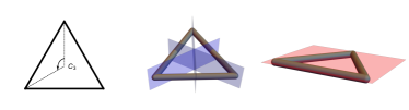
Figure 6: Symmetries of a triangle in the kagome lattice used to constrain the exchange Hamiltonian, Eq. (30) Essafi et al. (2017). These are: $C_{3}$ rotations around the center of the triangle, reflections in the planes perpendicular to each bond, and reflection in the plane of the lattice itself.

Figure 7: Global and local bases used in Eqs. (30)-(31), and numbering convention used for sites on a triangle.

Transforming to a local coordinate system, with local axes in the $xy$-plane ${\bf\hat{x}}_{i},{\bf\hat{y}}_{i}$ on each site of the triangle as shown in Fig. 7, while maintaining the same global ${\bf\hat{z}}$ axis, the coupling matrices become uniform:

$$\tilde{J}=R_{i}\cdot J_{ij}\cdot R^{T}_{j}=$$

$$\begin{pmatrix}-\frac{1}{2}\left(\sqrt{3}D_{z}+J_{\perp}\right)+t&\frac{1}{2}\left(-D_{z}+\sqrt{3}J_{\perp}\right)&0\\ \frac{1}{2}\left(D_{z}-\sqrt{3}J_{\perp}\right)&-\frac{1}{2}\left(\sqrt{3}D_{z}+J_{\perp}\right)-t&0\\ 0&0&J_{z}\end{pmatrix}.$$

(31)

In the special case $D_{z}=\sqrt{3}J_{\perp}$, this becomes an XYZ model with

$$J_{x}=-2J_{\perp}+t\,,\quad J_{y}=-2J_{\perp}-t\,.$$ (32)

This establishes that the XYZ model discussed in the main text occurs as a limit of the general symmetry-allowed anisotropic exchange Hamiltonian for kagome magnets.

Appendix B Derivation of the exact ground states

Here we show how to obtain analytic expressions for the ground states in the exactly solvable limits of the XYZ model.

The ground state wave functions are product states of the form Eq. (9) Such a wave function is completely determined (up to a global phase) by the expectation values of the spin components on each site:

$$\langle S^{x}_{i}\rangle=\frac{1}{2}\sin(\theta_{i})\cos(\phi_{i})\,,$$

$$\langle S^{y}_{i}\rangle=\frac{1}{2}\sin(\theta_{i})\sin(\phi_{i})\,,$$

$$\langle S^{z}_{i}\rangle=\frac{1}{2}\cos(\theta_{i}).$$ (33)

The vector $\langle{\bf S}_{i}\rangle=(\langle S^{x}_{i}\rangle,\langle S^{y}_{i}\rangle,\langle S^{z}_{i}\rangle)$ is constrained to lie on a sphere:

$$\langle S^{x}_{i}\rangle^{2}+\langle S^{y}_{i}\rangle^{2}+\langle S^{z}_{i}\rangle^{2}=1/4\,,\quad\forall\,i\,.$$ (34)

In the following, we find analytic expressions for $\langle{\bf S}_{i}\rangle$ for all product state ground states of the single triangle Hamiltonian, at the exactly solvable points of the XYZ model. The ground states on the lattice follow from this by tiling the lattice with single triangle solutions in the way described in the main text.

The exactly solvable parameter space is given by $J_{x}J_{y}+J_{y}J_{z}+J_{z}J_{x}=0$ and $J_{x}+J_{y}+J_{z}>0$. Setting $J_{x}+J_{y}+J_{z}=1$ as the unit of energy we can then write the exchange parameters as a function of a single variable $\kappa$:

$$J_{x/y} =\frac{1}{3}+\frac{1}{3}\cos(\kappa)\pm\frac{1}{\sqrt{3}}\sin(\kappa)\,,$$

$$J_{z} =\frac{1}{3}-\frac{2}{3}\cos(\kappa)\,.$$ (35)

The points $\kappa=0$, $2\pi/3$, and $4\pi/3$ correspond to the XXZ0 points along the ${\bf\hat{z}}$, ${\bf\hat{y}}$, and ${\bf\hat{x}}$ axis, respectively, whereas $\kappa=\pi/3$, $\pi$, and $5\pi/3$ correspond to the Ising points along the ${\bf\hat{x}}$, ${\bf\hat{z}}$, and ${\bf\hat{y}}$ axis, respectively. If we attribute $\beta=x\to 1$, $y\to 2$, and $z\to 3$, then the above can be compactly written as:

$$J_{\beta}=\frac{1}{3}-\frac{2}{3}\cos\left(\kappa+\frac{2\pi}{3}\beta\right)\,.$$ (36)

The above parameterisation has the nice property that it allows us to focus on the parameter range $\kappa\in[0,\pi/3]$, with the rest related to this range by a permutation of the $\{J\}$ coefficients and spin components. In particular:

$$(J_{x},J_{y},J_{z})\big{|}_{-\kappa}=(J_{y},J_{x},J_{z})\big{|}_{\kappa}\,,$$ (37)

$$(J_{x},J_{y},J_{z})\big{|}_{\kappa+2\pi/3}=(J_{y},J_{z},J_{x})\big{|}_{\kappa}\,.$$ (38)

This permutation symmetry (of the $x,y,z$ components) relates systems with different exchange coefficients and should not be conflated with the dynamical permutation symmetry of exchanging the spins on a triangle, whilst keeping $\{J\}$ the same. The latter we used in Section II.2 to derive the tiling rules.

Since the XXZ0 and Ising points were analyzed in the main text under Section II.1, below we focus on the case of generic $\kappa\in\langle 0,\pi/3\rangle$.

B.1 Method of Lagrange multipliers

For generic values of $\kappa$, not equal to $\mathbb{Z}\pi/3$, we find the ground state by minimising the expectation value of the energy, using Lagrange multipliers to enforce Eq. (34). If this expectation value $\langle\Psi|\mathcal{H}_{\text{XYZ}}|\Psi\rangle$ coincides with the known ground state energy $e_{0}=-\frac{1}{4}(J_{x}+J_{y}+J_{z})=-1/4$, then $\lvert\Psi\rangle$ is a ground state.

The energy of the product state can be written directly in terms of the spin expectation values:

$$E_{\Psi}=\langle\Psi|\mathcal{H}_{\text{XYZ}}|\Psi\rangle=\sum_{\langle ij\rangle}\sum_{\beta=x,y,z}J_{\beta}\langle S^{\beta}_{i}\rangle\langle S^{\beta}_{j}\rangle\,.$$ (39)

To simplify the notation, we will from this point forward denote $\langle S^{\beta}_{i}\rangle$ as $S^{\beta}_{i}$ and treat them as classical variables. The problem is then to minimize $E_{\Psi}$ with respect to the nine variables $S^{\beta}_{i}$ (three components $\beta$ on each of three sites of a triangle $i$), while respecting the three constraints Eq. (34). This can be achieved with the method of Lagrange multipliers.

We seek to minimize:

$$\begin{aligned} E^{\prime}=\frac{1}{4}&+\frac{1}{2}\sum_{i\neq j}\sum_{\beta=x,y,z}J_{\beta}S_{i}^{\beta}S_{j}^{\beta}\\ &-\frac{1}{2}\sum_{i}\mu_{i}\left({\bf S}_{i}^{2}-\frac{1}{4}\right)=0\,,\end{aligned}$$ (40)

$$\frac{\partial E^{\prime}}{\partial S_{i}^{\beta}}=0\,,\quad\forall\,i,\beta\,,$$ (41)

$$\frac{\partial E^{\prime}}{\partial\mu_{i}}=0,\quad\forall\,i\,,$$ (42)

where we have introduced three Lagrange multipliers $\mu_{i}$ to the energy, to satisfy Eq. (34).

Eq. (41) has the form of zero-eigenvalue equation for a block diagonal matrix

$${\mathcal{M}}\cdot\tilde{S} =0\,,$$ (43)

$$\tilde{S} =\left(S^{x}_{1}\ S^{x}_{2}\ S^{x}_{3}\ S^{y}_{1}\ S^{y}_{2}\ S^{y}_{3}\ S^{z}_{1}\ S^{z}_{2}\ S^{z}_{3}\right)^{T},$$ (44)

$$\mathcal{M} =\begin{pmatrix}M_{x}&0&0\\ 0&M_{y}&0\\ 0&0&M_{z}\end{pmatrix},\ M_{\beta}=\begin{pmatrix}-\mu_{1}&J_{\beta}&J_{\beta}\\ J_{\beta}&-\mu_{2}&J_{\beta}\\ J_{\beta}&J_{\beta}&-\mu_{3}\end{pmatrix}.$$

For there to be solutions of Eq. (43) where all spin components are finite on at least one spin in the triangle, we require that:

$$\det M_{\beta}=2J_{\beta}^{3}+J_{\beta}^{2}(\mu_{1}+\mu_{2}+\mu_{3})-\mu_{1}\mu_{2}\mu_{3}=0\,,\quad\forall\,\beta\,.$$

(46)

Acting on Eq. (43) from the left with $\tilde{S}$, and using the spin length constraints and the known ground state energy, gives us

$$\mu_{1}+\mu_{2}+\mu_{3}=-2(J_{x}+J_{y}+J_{z})=-2\,.$$ (47)

Substituting Eq. (47) in to Eq. (46), gives the relation:

$$\mu_{1}\mu_{2}\mu_{3}=2J_{\beta}^{2}(J_{\beta}-1)=-\frac{8}{27}\cos^{2}\left(\frac{3\kappa}{2}\right)\,.$$ (48)

Eqs. (47) and (48) are sufficient to guarantee the satisfaction of all three conditions in Eq. (46).

The next step is then to solve Eqs. (47) and (48) to give expressions for $\mu$ in terms of $\kappa$. To do this, we write $\mu_{j}$ in terms of polar coordinates, an angle $u$ and radius $r(u)$,

$$\mu_{j}=-\frac{2}{3}-\frac{2}{3}r(u)\cos\left(u+\frac{2\pi j}{3}\right)\,.$$ (49)

This solves Eq. (47), and Eq. (48) now gives a cubic equation for $r(u)$:

$$\cos(3u)\,r^{3}-3\,r^{2}+4\sin^{2}\left(\frac{3\kappa}{2}\right)=0\,.$$ (50)

For general $u\neq\pi/6+\mathbb{Z}\pi/3$, that is $\cos(3u)\neq 0$, the above equation has three real roots $r_{n}(u,\kappa)$, $n=0,1,2$, given by Viète’s formula:

$$r_{n}(u)=\sec(3u)-2|\sec(3u)|\cos\left(\Phi(u)+\frac{2\pi n}{3}\right)\,,$$ (51)

$$\Phi(u)=\frac{1}{3}{\rm arccos}\left[{\rm sgn}(\cos(3u))\left[-1+2\cos^{2}(3u)\sin^{2}\left(3\kappa/2\right)\right]\right]\,.$$

The identities ${\rm arccos}(1-2x^{2})=2|{\rm arcsin}(x)|$ and ${\rm arccos}(x)+{\rm arccos}(-x)=\pi$, when combined with a piecewise redefinition of $n$, allow us to further simplify the above to:

$$r_{n}(u)=\sec(3u)\left[1+2\cos\left[\frac{2}{3}{\rm arcsin}(\cos(3u)\sin(3\kappa/2))+\frac{2\pi n}{3}\right]\right]\,.$$

(53)

Since we’re using polar coordinates to express $\mu_{j}$ in Eq. (49), $(r,u)$ and $(-r,u+\pi)$ represent the same $\mu_{j}$ and the $n=1$ and $n=2$ radial solutions are equivalent. Thus there are only two distinct solutions, having $n=0$ and $1$.

Some properties of $r_{n}(u,\kappa)$ and $\mu_{j}(u,n,\kappa)$:

• Since $r_{n}(u,\kappa)$ depends on $u$ only through $\cos(3u)$, it satisfies $r_{n}(u,\kappa)=r_{n}(-u,\kappa)=r_{n}(u+2\pi/3,\kappa)$ and therefore $\mu_{j}$ satisfies $\mu_{j}(u,n,\kappa)=\mu_{j+3}(u,n,\kappa)=\mu_{j+1}(u-2\pi/3,n,\kappa)=\mu_{-j}(-u,n,\kappa)$. Hence results derived for $\mu_{3}$ transfer to $\mu_{1}$ and $\mu_{2}$ (i.e., $\mu_{1}$ and $\mu_{2}$ do not need to be considered separately).

• Only for the XXZ0 points, $\kappa=\mathbb{Z}2\pi/3\implies\sin(3\kappa/2)=0$, does Eq. (50) have a (double) solution $r_{1/2}=0$. For all other $\kappa\neq\mathbb{Z}2\pi/3$ and $u\in\mathbb{R}$, $r_{n}(u,\kappa)\neq 0$. The other solution at the XXZ0 points is $r_{0}=3/\cos(3u)$.

• At the Ising points, $\kappa=\pi/3+\mathbb{Z}2\pi/3\implies\sin^{2}(3\kappa/2)=1$, the three solutions of Eq. (50) can be written as $r^{{\rm Ising}}_{n}(u)=-1/\cos(u+2\pi n/3)$. A piecewise patching of the different $n$ solutions from Eq. (53) is needed to construct these smooth $r^{{\rm Ising}}_{n}$.

• By studying the limit $u\to\pi/6+\mathbb{Z}\pi/3$ of $r_{n}(u)$ where $\sec(3u)$ diverges, one may confirm that the $n=0$ solution of Eq. (53) diverges there, whereas $r_{n=1}=-(2/\sqrt{3})\sin(3\kappa/2)$ at these points. The latter value also follows directly from Eq. (50). As for $\mu_{j}$, the $\cos(u+2\pi j/3)$ from Eq. (49) eliminates some of the $n=0$ divergences. Specifically, for $\mu_{3}(n=0)$ the only unremovable poles are at $u=\pm\pi/6$ and $u=\pm 5\pi/6$ (for all $\kappa$).

• At the Ising points $\kappa=\pi/3+\mathbb{Z}2\pi/3$, ${\rm arcsin}(\cos(3u))$ is a sawtooth-like function that is not smooth at $u=\mathbb{Z}\pi/3$. Consequently, $r_{n=0}(u)$ as given by Eq. (53) is not smooth at $(u,\kappa)=(\mathbb{Z}\pi/3,\pi/3+\mathbb{Z}2\pi/3)$, and $r_{n=1}(u)$ is not smooth at $(u,\kappa)=(\pi/3+\mathbb{Z}2\pi/3,\pi/3+\mathbb{Z}4\pi/3)$ and $(\mathbb{Z}2\pi/3,\pi+\mathbb{Z}4\pi/3)$. For all other $\kappa$, the functions $r_{n}(u,\kappa)$ and $\mu_{j}(u,n,\kappa)$ are smooth in $u$ on their whole domain of definition (which for $n=0$ excludes certain singularities). Likewise, for fixed $u=\mathbb{Z}\pi/3$, ${\rm arcsin}(\sin(3\kappa/2))$ from the $r_{n}(\kappa)$ are not smooth at the same $(u,\kappa)$ points from above. For all other fixed $u$, the functions $r_{n}(u,\kappa)$ and $\mu_{j}(u,n,\kappa)$ are smooth in $\kappa$ for all $\kappa\in\mathbb{R}$.

• Lastly, for a fixed $n$, $r_{n}(u,\kappa)$ and $\mu_{j}(u,n,\kappa)$ as functions of $(u,\kappa)$ are smooth everywhere on their domains of definitions, excluding the cusps listed under (v). This is a stronger statement than being smooth in only $u$ or $\kappa$, and it follows from the structure of Eqs. (53) and (49). With that said, in the arguments that follow we shall only be needing the piecewise continuity and differentiability in $u$ of these functions.

With the values of $\mu_{j}$ determined, the vector of spin components $\tilde{S}$ [Eq. (44)] is given by a linear combination of the null vectors of $\mathcal{M}$. Row reduction of $M_{\beta}$ gives

$$M_{\beta}\sim\begin{pmatrix}J_{\beta}+\mu_{1}&-(J_{\beta}+\mu_{2})&0\\ 0&J_{\beta}+\mu_{2}&-(J_{\beta}+\mu_{3})\\ -\mu_{1}&J_{\beta}&J_{\beta}\\ \end{pmatrix}$$

$$\sim\begin{pmatrix}J_{\beta}+\mu_{1}&-(J_{\beta}+\mu_{2})&0\\ 0&J_{\beta}+\mu_{2}&-(J_{\beta}+\mu_{3})\\ 0&0&0\\ \end{pmatrix},$$ (54)

where in the second step we have used Eq. (46) and assumed that at least two $i$ out of three satisfy $J_{\beta}+\mu_{i}\neq 0$. It turns out that for all $\kappa$, there are special values of $u$, denoted $u^{*}$, for which two $J_{\beta}+\mu_{i}$ (with the same $\beta$) vanish, invalidating the second step above.

For generic $\kappa\neq\mathbb{Z}\pi/3$ (i.e., not Ising or XXZ0 points), however, these special $u^{*}$ are restricted to a discrete number of points. Although not obvious, all $\tilde{S}$ solutions of these special $u^{*}$ can be obtained by a limiting procedure of the generic $u$ solutions.

Below we first determine when $J_{\beta}+\mu_{i}=0$ and find that these special $u^{*}$ are, for generic $\kappa$, given by $u^{*}=\mathbb{Z}\pi/3$. Then we find the spins $\tilde{S}$ at these special $u^{*}$ explicitly to confirm that there are no points isolated from the generic $u$ solutions. Lastly, we find the $\tilde{S}$ for generic $u$.

B.2 Finding the special $u^{*}$

In the coming two sections, the functions $J_{\beta}+\mu_{i}$ shall play a prominent role, so we introduce

$$a_{\beta i}(u,n,\kappa)=\frac{1}{2}\big{(}J_{\beta}(\kappa)+\mu_{i}(u,n,\kappa)\big{)}\,.$$ (55)

Special $u^{*}$ we define as those $u$ for which least one $a_{\beta i}(u^{*})$ vanishes. Let us consider the case where $a_{x1}=0$. Then $\mu_{1}=-J_{x}$ and one may easily solve Eqs. (47) and (48) to get $(\mu_{2}+J_{x})(\mu_{2}+2-2J_{x})=0$ and $\mu_{3}=J_{x}-2-\mu_{2}$. Thus $\mu_{1}=-J_{x}$ implies that either $\mu_{2}=-J_{x}$ and $\mu_{3}=2(J_{x}-1)$, or $\mu_{2}=2(J_{x}-1)$ and $\mu_{3}=-J_{x}$. Focusing on the case $\mu_{1}=\mu_{2}=-J_{x}$ and $\mu_{3}=2(J_{x}-1)$, we see that $a_{x1}=a_{x2}=0$ and $a_{x3}=3(J_{x}-2/3)\neq 0$ when we’re not at a XXZ0 point. We may therefore conclude that $a_{\beta i}$ always vanish in pairs (with the same $\beta$), but for generic $\kappa$ never in triplets (i.e., $a_{\beta 1}=a_{\beta 2}=a_{\beta 3}=0$ never happens).

These special points $\mu_{1}=\mu_{2}=-J_{x}$ and $\mu_{3}=2(J_{x}-1)$, moreover, coincide with the extrema of $\mu_{3}$. To prove this, we differentiate Eqs. (47) and (48) to get, for all $u$,

$$\partial_{u}\mu_{1}+\partial_{u}\mu_{2}+\partial_{u}\mu_{3} =0\,,$$ (56)

$$(\partial_{u}\mu_{1})\mu_{2}\mu_{3}+\mu_{1}(\partial_{u}\mu_{2})\mu_{3}+\mu_{1}\mu_{2}(\partial_{u}\mu_{3}) =0\,.$$ (57)

By substituting $\mu_{1}=\mu_{2}=-J_{x}$, $\mu_{3}=2(J_{x}-1)$ in to the above, one obtains $J_{x}(J_{x}-2/3)\partial_{u}\mu_{3}(u^{*})=0$. Since $J_{\beta}=0$ only at the Ising points, and $J_{\beta}=2/3$ only at the XXZ0 points, we conclude that for generic $\kappa$, $\partial_{u}\mu_{3}(u^{*})=0$.

The converse statement also holds. That is, $\partial_{u}\mu_{3}(u^{*})=0$ implies that for at least one $\beta$, $\mu_{1}(u^{*})=\mu_{2}(u^{*})=-J_{\beta}$ and $\mu_{3}(u^{*})=2(J_{\beta}-1)$. To prove this, we use $\partial_{u}\mu_{3}(u^{*})=0$ in Eqs. (56) and (57) to obtain $(\mu_{1}-\mu_{2})\mu_{3}\partial_{u}\mu_{1}=0$. The case $\mu_{3}=0$ is forbidden for non-Ising $\kappa$ because of Eq. (48). The case $\partial_{u}\mu_{1}=\partial_{u}\mu_{2}=\partial_{u}\mu_{3}=0$ happens only for the XXZ0 point with $r=0$. The generic case $\mu_{1}=\mu_{2}$, when combined with Eqs. (47) and (48), yields $(\mu_{1}+J_{x})(\mu_{1}+J_{y})(\mu_{1}+J_{z})=0$ and $\mu_{3}=-2\mu_{1}-2$, which is the desired result.

Using $\partial_{u}\mu_{3}(u^{*})=0$ one can find the special $u^{*}$ without solving any complicated algebraic equations that include the expression (53). First, we differentiate the cubic equation (50) and solve for $\partial_{u}r$,

$$\frac{\partial_{u}r}{r}=\frac{r\sin(3u)}{r\cos(3u)-2}\,.$$ (58)

Next, we differentiate the definition (49) of $\mu_{j}$ and use $\partial_{u}\mu_{3}(u^{*})=0$ to get

$$\frac{\partial_{u}r(u^{*})}{r(u^{*})}=\frac{\sin(u^{*})}{\cos(u^{*})}\,.$$ (59)

By combining the above two equations, one obtains the desired equation

$$(r(u^{*})\cos(u^{*})+1)\sin(u^{*})=0\,.$$ (60)

The only case when $r(u^{*})=-1/\cos(u^{*})$ is a solution of the cubic equation (50) is at the Ising points. Thus, for generic $\kappa$, $a_{\beta 1}=a_{\beta 2}=0$ occurs only at $u^{*}=\mathbb{Z}\pi$. Analogously, $a_{\beta 1}=a_{\beta 3}=0$ occurs only at $u^{*}=2\pi/3+\mathbb{Z}\pi$, and $a_{\beta 2}=a_{\beta 3}=0$ occurs only at $u^{*}=\pi/3+\mathbb{Z}\pi$. Altogether, the special $u^{*}$ are given by $\mathbb{Z}\pi/3$.

These special $u^{*}$ also arise when finding the $\tilde{S}$. The limiting condition that arises in that context is $|a_{\beta i}|=|a_{\beta j}|$. Focusing on the case $i=1,j=2$, the question is when is $|a_{\beta 1}|=|a_{\beta 2}|$ for some $\beta$? To answer this, one must consider two cases, $a_{\beta 1}=+a_{\beta 2}\implies\mu_{1}=\mu_{2}$ and $a_{\beta 1}=-a_{\beta 2}\implies 2J_{\beta}+\mu_{1}+\mu_{2}=0$. In either case, after solving with Eqs. (47) and (48), one finds that $\mu_{1}=\mu_{2}=-J_{\beta^{\prime}}$ and $\mu_{3}=2(J_{\beta^{\prime}}-1)$, for some potentially different $\beta^{\prime}$. Thus $|a_{\beta 1}|=|a_{\beta 2}|$ happens only at $u^{*}=\mathbb{Z}\pi$, and more generally $|a_{\beta i}|=|a_{\beta j}|$ occurs only at $u^{*}=\mathbb{Z}\pi/3$. Indeed, when we know that, say, $|a_{x1}|=|a_{x2}|$, then $|a_{y1}|=|a_{y2}|$ and $|a_{z1}|=|a_{z2}|$ must hold as well, and only one of these three vanishes, the others being finite; $|a_{x3}|,|a_{y3}|,|a_{z3}|$ also must be non-zero. All of this holds for generic $\kappa\neq\mathbb{Z}\pi/3$.

B.3 Ground states for special $u^{*}=\mathbb{Z}\pi/3$ and $0<\kappa<\pi/3$

Let us consider a special point $u^{*}$ where $|a_{\gamma i}|=|a_{\gamma j}|=0$ for a fixed $n=0,1$. The remaining component and spin indices we shall denote $\beta_{1},\beta_{2}$ and $k$, respectively, so that $(\beta_{1},\beta_{2},\gamma)$ and $(i,j,k)$ are permutations of $(x,y,z)$ and $(1,2,3)$, respectively. We moreover consider only the range $0<\kappa<\pi/3$, since the parameterisation permutation symmetry [Eqs. (37)-(38)] maps this region to all other generic $\kappa$.

From the previous section we know that $|a_{\beta_{1}i}|=|a_{\beta_{1}j}|\neq 0$, $|a_{\beta_{2}i}|=|a_{\beta_{2}j}|\neq 0$, and $|a_{\beta_{1}k}|,|a_{\beta_{2}k}|,|a_{\gamma k}|\neq 0$ are all non-zero. In light of Eq. (54), the null vectors of $M_{\beta_{1}}$ and $M_{\beta_{2}}$ are given by

$$V_{\beta}=2\begin{pmatrix}(J_{\beta}+\mu_{1})^{-1}\\ (J_{\beta}+\mu_{2})^{-1}\\ (J_{\beta}+\mu_{3})^{-1}\end{pmatrix}=\begin{pmatrix}a_{\beta 1}^{-1}\\ a_{\beta 2}^{-1}\\ a_{\beta 3}^{-1}\end{pmatrix}\,,$$ (61)

whereas the null vector of $M_{\gamma}$ has the components $(V_{\gamma})_{i}=-(V_{\gamma})_{j}=1$ and $(V_{\gamma})_{k}=0$.

Since $\tilde{S}$ is a null vector of $\mathcal{M}$ [Eq. (43)], we may write it as:

$$\tilde{S}=\frac{1}{2}\begin{pmatrix}X_{x}V_{x}\\ X_{y}V_{y}\\ X_{z}V_{z}\end{pmatrix}\,,$$ (62)

where the coefficients $X_{\beta}$ are fixed by the spin normalization constraints [Eq. (34)].

Because of the relations among $\{a_{\beta i}\}$, only two of the three spin normalization constraints are independent, to wit

$$\frac{X^{2}_{\beta_{1}}}{|a_{\beta_{1}i}|^{2}}+\frac{X^{2}_{\beta_{2}}}{|a_{\beta_{2}i}|^{2}}+X^{2}_{\gamma} = 1\,,$$ (63)

$$\frac{X^{2}_{\beta_{1}}}{|a_{\beta_{1}k}|^{2}}+\frac{X^{2}_{\beta_{2}}}{|a_{\beta_{2}k}|^{2}} = 1\,.$$ (64)

Eq. (63) defines an ellipsoid and Eq. (64) a cylinder. These two intersect at:

$$X_{\beta_{1}}(v)=a_{\beta_{1}k}\cos(v)\,,$$ (65)

$$X_{\beta_{2}}(v)=a_{\beta_{2}k}\sin(v)\,,$$ (66)

$$X_{\gamma}(v)=\pm\sqrt{1-\left(\frac{a_{\beta_{1}k}}{a_{\beta_{1}i}}\right)^{2}\cos^{2}(v)-\left(\frac{a_{\beta_{2}k}}{a_{\beta_{2}i}}\right)^{2}\sin^{2}(v)}\,,$$

(67)

and the spins are given by

$${\bf S}_{i}=\frac{1}{2}\begin{pmatrix}X_{\beta_{1}}/a_{\beta_{1}i}\\ X_{\beta_{2}}/a_{\beta_{2}i}\\ +X_{\gamma}\end{pmatrix}\,,\ \ {\bf S}_{j}=\frac{1}{2}\begin{pmatrix}X_{\beta_{1}}/a_{\beta_{1}j}\\ X_{\beta_{2}}/a_{\beta_{2}j}\\ -X_{\gamma}\end{pmatrix}\,,$$

$${\bf S}_{k}=\frac{1}{2}\begin{pmatrix}X_{\beta_{1}}/a_{\beta_{1}k}\\ X_{\beta_{2}}/a_{\beta_{2}k}\\ 0\end{pmatrix}\,,$$ (68)

where the rows represent the $\beta_{1}$, $\beta_{2}$, and $\gamma$ components of the spins.

What these equations represent depends on the ratios $(a_{\beta_{1}k}/a_{\beta_{1}i})^{2}$ and $(a_{\beta_{2}k}/a_{\beta_{2}i})^{2}$. We have three cases to consider:

• When $(a_{\beta_{1}k}/a_{\beta_{1}i})^{2}>1$ and $(a_{\beta_{2}k}/a_{\beta_{2}i})^{2}>1$, the $X_{\gamma}$ are imaginary and there are no $\tilde{S}$ that satisfy the spin normalization constraints. Said differently, the ellipsoid [Eq. (63)] and cylinder [Eq. (64)] do not intersect. On $0<\kappa<\pi/3$, this is the case for the $n=0$ solutions on all $u^{*}=\mathbb{Z}\pi/3$.

• When $(a_{\beta_{1}k}/a_{\beta_{1}i})^{2}<1$ and $(a_{\beta_{2}k}/a_{\beta_{2}i})^{2}<1$, $X_{\gamma}$ is real for all $v$, and Eqs. (65)-(67) parametrizes two ($\pm$) closed lines. Once projected on to the $i,j,k$ spin spheres, one obtains lines that have a circular shape in the $\beta_{1}\beta_{2}$ plane. On $0<\kappa<\pi/3$, this is the case for the $n=1$ solutions with $u^{*}=\mathbb{Z}2\pi/3$. In detail, $(i,j)=(1,2)$ for $u^{*}=0$, $(1,3)$ for $u^{*}=2\pi/3$, and $(2,3)$ for $u^{*}=4\pi/3$; $(\beta_{1},\beta_{2},\gamma)=(y,z,x)$ in all cases.

• When $(a_{\beta_{1}k}/a_{\beta_{1}i})^{2}>1$ and $(a_{\beta_{2}k}/a_{\beta_{2}i})^{2}<1$, it is better to eliminate $X_{\beta_{2}}$ from Eq. (63), giving

  $$X_{\gamma}(v)=\sqrt{1-(a_{\beta_{2}k}/a_{\beta_{2}i})^{2}}\,\cos(v)\,,$$ (69)

  $$X_{\beta_{1}}(v)=\sqrt{\frac{(a_{\beta_{2}i})^{2}-(a_{\beta_{2}k})^{2}}{(a_{\beta_{2}i}/a_{\beta_{1}i})^{2}-(a_{\beta_{2}k}/a_{\beta_{1}k})^{2}}}\,\sin(v)\,,$$ (70)

  $$X_{\beta_{2}}(v)=$$

  $$\pm a_{\beta_{1}k}\sqrt{\frac{1-(a_{\beta_{1}i}/a_{\beta_{1}k})^{2}\sin^{2}(v)-(a_{\beta_{2}k}/a_{\beta_{2}i})^{2}\cos^{2}(v)}{(a_{\beta_{1}k}/a_{\beta_{2}k})^{2}-(a_{\beta_{1}i}/a_{\beta_{2}i})^{2}}}\,.$$

  The above is again well-defined for all $v$, and parametrizes two closed lines. Once projected on to the $i,j$ spheres, we get lines circular in the $\gamma\beta_{1}$ plane. On the $k$ sphere, we get a line squashed along the $\gamma$ direction, $S^{\gamma}_{k}=0$. On $0<\kappa<\pi/3$, this is the case for the $n=1$ solutions with $u^{*}=\pi/3+\mathbb{Z}2\pi/3$. In detail, $(i,j)=(2,3)$ for $u^{*}=0$, $(1,2)$ for $u^{*}=2\pi/3$, and $(1,3)$ for $u^{*}=4\pi/3$; $(\beta_{1},\beta_{2},\gamma)=(z,x,y)$ in all cases.

Lastly, let us comment on how the $i,j,k,\beta_{1},\beta_{2},\gamma$ are determined. Since from previous study we know that $|a_{\beta i}|$ are continuous functions of $\kappa$ and that only at the special Ising and XXZ0 points may additional $|a_{\beta i}|$ coincide or vanish, it follows that it is sufficient to determine the $i,j,k,\beta_{1},\beta_{2},\gamma$ for a given $u^{*}\in\mathbb{Z}\pi/3$ at one $\kappa\in\langle 0,\pi/3\rangle$ to know these indices across this whole range. That is, because of discreteness and continuity, these indices may only change at $\kappa=\mathbb{Z}\pi/3$.

B.4 Ground states for generic $u\neq\mathbb{Z}\pi/3$ and $0<\kappa<\pi/3$

For a generic $u$ and $\kappa$, the null vectors of each $3\times 3$ submatrix $M_{\beta}$ are always given by Eq. (61), and $\tilde{S}$ can again be written as given in Eq. (62).

The allowed values of $X_{\beta}$ are determined by the intersection of 3 ellipsoids that follow from the spin normalization constraints:

$$\frac{X_{x}^{2}}{a_{xi}^{2}}+\frac{X_{y}^{2}}{a_{yi}^{2}}+\frac{X_{z}^{2}}{a_{zi}^{2}}=1\,,\quad i=1,2,3\,,$$ (72)

with semi-axis lengths $|a_{\beta i}|$ [Eq. (55)], known to all be non-zero for $u\neq\mathbb{Z}\pi/3$.

One might expect Eqs. (72) to give eight solutions for $X_{\beta}$ for each $\kappa,u,n$ given by

$$\begin{pmatrix}X_{x}^{2}\\ X_{y}^{2}\\ X_{z}^{2}\end{pmatrix}=\mathcal{A}^{-1}\cdot\begin{pmatrix}1\\ 1\\ 1\end{pmatrix}\,,$$ (73)

$$\mathcal{A}=\begin{pmatrix}\left(1/a_{x1}\right)^{2}&\left(1/a_{y1}\right)^{2}&\left(1/a_{z1}\right)^{2}\\ \left(1/a_{x2}\right)^{2}&\left(1/a_{y2}\right)^{2}&\left(1/a_{z2}\right)^{2}\\ \left(1/a_{x3}\right)^{2}&\left(1/a_{y3}\right)^{2}&\left(1/a_{z3}\right)^{2}\end{pmatrix}\,.$$ (74)

However, the matrix $\mathcal{A}$ actually has a vanishing determinant, signifying that one of the three constraints in Eq. (72) is linearly dependent on the other two.

In the previous section, we have already seen this linear dependence make the $i,j$ constraints of Eq. (63) identical. Although we are presently unable to give an analytic proof of the statement $\det\mathcal{A}=0$ for generic $u$, we have verified it numerically for the full spectrum of possible values of $\kappa,u,n$ and it holds for all cases.

Given that only two of the constraints in Eq. (72) are linearly independent, there exist one-parameter families of solutions for $X_{\beta}$. We will parametrize these families with a continuous parameter $v$. Combined with the fact that $u$ is also a continuous parameter, this means that for all sets of generic exchange parameters $\{J\}$ [Eq. (36) with $\kappa\neq\mathbb{Z}\pi/3$], the set of ground states has two continuous free parameters, $u$ and $v$.

For two ellipsoids with semi-axis lengths $(|a_{x1}|,|a_{y1}|,|a_{z1}|)$ and $(|a_{x2}|,|a_{y2}|,|a_{z2}|)$ (both having principal semi-axes aligned along the coordinate directions $x,y,z$) to intersect, each ellipsoid must have at least one axis whose length is longer than the corresponding axis of the other ellipsoid (i.e., we cannot have $|a_{x1}|>|a_{x2}|$, $|a_{y1}|>|a_{y2}|$, $|a_{z1}|>|a_{z2}|$).

As previously established, $|a_{\beta i}|$ are piecewise continuous functions of $u$ and $\kappa$ that can (for generic $\kappa$) intersect only at the special $u^{*}=\mathbb{Z}\pi/3$ points. Thus if we consider, for instance, $u\in\langle 0,\pi/3\rangle$ and $\kappa\in\langle 0,\pi/3\rangle$, then for this whole range all $|a_{\beta i}|$ differ and, moreover, the corresponding ellipsoids must intersect, or not, in the same way. When one considers the $n=0$ solution, one must also pay attention to the divergences of $|a_{\beta i}|$ that happen at $u_{\rm div}=\pi/6+\mathbb{Z}\pi/3$.

After analysing the various cases for $0<\kappa<\pi/3$, one finds that the $n=0$ ellipsoids with semi-axes $|a_{\beta i}(u,n=0,\kappa)|$ never intersect. This agrees with the previous section where the $n=0$ case also could not satisfy the spin normalization constraints (the cylinder and ellipsoid did not intersect).

As for the $n=1$ case, on the interval $0<u<\pi$ (not including the special $\mathbb{Z}\pi/3$), one finds that

$$|a_{x1}|<|a_{x2}|\,,\ |a_{y1}|>|a_{y2}|\,,\ |a_{z1}|>|a_{z2}|\,,$$ (75)

holds, whereas for $\pi<u<2\pi$, the reverse holds:

$$|a_{x1}|>|a_{x2}|\,,\ |a_{y1}|<|a_{y2}|\,,\ |a_{z1}|<|a_{z2}|\,.$$ (76)

In either case, one may solve Eq. (72) with $i=1$ for $X_{x}$,

$$X_{x}=\pm a_{x1}\sqrt{1-\left(\frac{X_{y}}{a_{y1}}\right)^{2}-\left(\frac{X_{z}}{a_{z1}}\right)^{2}}\,\,,$$ (77)

and then substitute in to Eq. (72) with $i=2$, yielding

$$\left(\frac{X_{y}}{b_{y,x}^{2,1}}\right)^{2}+\left(\frac{X_{z}}{b_{z,x}^{2,1}}\right)^{2}=1\,,$$ (78)

$$b_{\beta,\gamma}^{i,j}=b_{\gamma,\beta}^{j,i}=\sqrt{\frac{(a_{\gamma j})^{2}-(a_{\gamma i})^{2}}{\left(a_{\gamma j}/a_{\beta j}\right)^{2}-\left(a_{\gamma i}/a_{\beta i}\right)^{2}}}\,\,.$$ (79)

Note how the inequalities (75) and (76) ensure that $b^{2,1}_{y,x}>0$ and $b^{2,1}_{z,x}>0$.

Altogether, the solutions of the three ellipsoid equations can be parametrized as:

$$X_{x}(u,v,\kappa)=$$

$$\pm a_{x1}(u,n=1,\kappa)\sqrt{1-\left(\frac{b^{2,1}_{y,x}}{a_{y1}}\right)^{2}\cos^{2}(v)-\left(\frac{b^{2,1}_{z,x}}{a_{z1}}\right)^{2}\sin^{2}(v)}\,,$$

(80)

$$X_{y}(u,v,\kappa)=+b^{2,1}_{y,x}(u,n=1,\kappa)\cos(v)\,,\quad$$ (81)

$$X_{z}(u,v,\kappa)=+b^{2,1}_{z,x}(u,n=1,\kappa)\sin(v)\,.\quad$$ (82)

If we consider the $\tilde{S}$ that the above solutions for $X_{\beta}$, when combined with Eqs. (33), (44), and (62), give, then one finds that for a fixed sign of $X_{x}$ these solutions are discontinuous at $u=\mathbb{Z}2\pi/3$. The cause is the fact that $X_{x}$ always has the same sign, whereas $a_{xi}$, and therefore $S^{x}_{i}$, change their sign at $u=\mathbb{Z}2\pi/3$.

If one tries to find a sign convention that preserves continuity, then one finds that the six patches of length $2\pi/3$ that Eqs. (80)-(82) yield combine in to one periodic patch of length $4\pi$.

In addition to the above, if one considers $\tilde{S}$ for a fixed $v$ as a function of $u$, the $+$ sign convention in Eq. (81) again gives discontinuities, but this time at $u=\pi/3+\mathbb{Z}2\pi/3$ and in the $S^{y}_{i}$ components of the spins. A simple sign change eliminates these.

In summary, the $X_{\beta}$, now named $X,Y,Z$, that give a continuous parameterisation of the ground state manifold are

$$X(u,v,\kappa)={\rm sgn}\left[\sin(3u/2)\right]a_{x1}(u,\kappa)\times$$

$$\qquad\sqrt{1-\left(\frac{b^{2,1}_{y,x}}{a_{y1}}\right)^{2}\cos^{2}(v)-\left(\frac{b^{2,1}_{z,x}}{a_{z1}}\right)^{2}\sin^{2}(v)}\,,$$ (83)

$$Y(u,v,\kappa)={\rm sgn}\left[\cos(3u/2)\right]b^{2,1}_{y,x}(u,\kappa)\cos(v)\,,$$ (84)

$$Z(u,v,\kappa)=+b^{2,1}_{z,x}(u,\kappa)\sin(v)\,,$$ (85)

where $u$ spans $[0,4\pi]$ and $v$ spans $[0,2\pi]$. By substituting in to Eq. (62), one obtains the desired values of all possible spins, and through Eq. (33) product states, that are in the ground state:

$${\bf S}_{1}(u,v,\kappa)=\frac{1}{2}\begin{pmatrix}\displaystyle\frac{X(u,v,\kappa)}{a_{x1}(u,\kappa)}\\ \displaystyle\frac{Y(u,v,\kappa)}{a_{y1}(u,\kappa)}\\ \displaystyle\frac{Z(u,v,\kappa)}{a_{z1}(u,\kappa)}\end{pmatrix}\,,$$ (86)

$${\bf S}_{2}(u,v,\kappa)=\frac{1}{2}\begin{pmatrix}\displaystyle\frac{X(u,v,\kappa)}{a_{x2}(u,\kappa)}\\ \displaystyle\frac{Y(u,v,\kappa)}{a_{y2}(u,\kappa)}\\ \displaystyle\frac{Z(u,v,\kappa)}{a_{z2}(u,\kappa)}\end{pmatrix}\,,$$ (87)

$${\bf S}_{3}(u,v,\kappa)=\frac{1}{2}\begin{pmatrix}\displaystyle\frac{X(u,v,\kappa)}{a_{x3}(u,\kappa)}\\ \displaystyle\frac{Y(u,v,\kappa)}{a_{y3}(u,\kappa)}\\ \displaystyle\frac{Z(u,v,\kappa)}{a_{z3}(u,\kappa)}\end{pmatrix}\,.$$ (88)

The above expressions are valid even at the special $u$ points if one takes a careful limiting procedure $u\to u^{*}\in\mathbb{Z}\pi/3$. What one obtains through such a limiting procedure agrees with the solutions derived in the previous section explicitly. This confirms that the above solutions exhaust the manifold of all product state ground states for $\kappa\neq\mathbb{Z}\pi/3$.

In the Supplementary Material sup , the reader may also find animations of the parameterisation from Eqs. (86)-(88) for $\kappa=0.1,\pi/6,0.9$. ”In the animations, two rows are drawn with three spin spheres and one $\mathcal{M}$ torus in each. In the upper row, lines of constant $u$ are drawn whose coloring indicates how $v$ is varied along them. In the lower row, $v$ is held constant and $u$ is varied.”

Appendix C Topology of the manifold of exact product ground states on a single triangle

In the previous section, we have found explicit parameterisations of all possible product states [Eq. (9)] that are grounds states of a single triangle. That is, at the points in the $\{J\}$ parameter space where the ground state is six-fold degenerate [Eq. (35)], we have found that this six-dimensional subspace of ground states includes a two-dimensional submanifold of separable states. Here we shortly discuss the topology of this separable ground state manifold $\mathcal{M}$.

The manifold $\mathcal{M}$ can be looked at as a submanifold embedded in the quantum space of ground state rays $\mathbb{C}\mathbf{P}^{5}=\mathbb{C}^{6}/{\sim}=\mathcal{S}^{11}/{\rm U}(1)$, but also as a submanifold embedded in the classical configuration space $\mathcal{S}^{2}\times\mathcal{S}^{2}\times\mathcal{S}^{2}$. The latter is just the statement that the product states are in correspondence with a state of classical vector spins, with components corresponding to the expectation values of the spin operators.

Although a small portion of $\mathbb{C}\mathbf{P}^{5}$, superpositions of separable states contained in $\mathcal{M}$ are in fact sufficient to describe all ground states on a single triangle. For the Ising and XXZ0 points, this can be verified explicitly, whereas for generic $\kappa$ we have verified this statement numerically for all $\kappa$: by taking six or more random points of $\mathcal{M}$ and calculating their corresponding quantum state vectors, one finds that the rank of these vectors is always six.

As shown in Fig. (2), the $\mathcal{M}$ of Ising and XXZ0 points are made of a series of spheres that touch neighbors in just such a way that together they resemble a wreath. In general, upon varying $\kappa$, the instabilities that these points of contact represent can be resolved by either combining or disconnecting these spheres. Because of the spin permutation $({\bf S}_{1},{\bf S}_{2},{\bf S}_{3})\mapsto({\bf S}_{\pi(1)},{\bf S}_{\pi(2)},{\bf S}_{\pi(3)})$ and inversion ${\bf S}_{i}\mapsto-{\bf S}_{i}$ symmetries, what happens at one junction must happen at all the other junctions.

Since there are no special $\kappa$ points besides these points, and there is no continuous way one can transform six disjoint spheres in to two touching spheres, it seems intuitively clear that the spheres must combine into one torus. And indeed, in our exact solution we have found that (for generic $\kappa$) $\mathcal{M}$ can be smoothly parametrized with two periodic parameters $u\in[0,4\pi]$ and $v\in[0,2\pi]$. Thus, $\mathcal{M}$ is topologically a torus. We have also verified this numerically (see next section for details).

Although both the Ising and XXZ0 points arise from a thinning out of the torus $\mathcal{M}$ at certain rings, for the Ising points the thinning happens at constant $u$, while for the XXZ0 points the thinning happens for constant $v$. This should be clearly visible in the animations of $\mathcal{M}$, available in the Supplementary Material sup .

Let us also comment on the mapping ${\bf S}_{1}\colon\mathcal{M}\to\mathcal{S}^{2}$. For generic $\kappa$, the Brouwer degree of this mapping is ${\rm deg}\,{\bf S}_{1}=\frac{1}{4\pi}\int_{\mathcal{M}}d\Omega_{1}=2$, where $d\Omega_{1}$ is the spherical angle two-form. Because of the parameterisation permutation symmetry [Eqs. (37)-(38)] and smoothness in $\kappa$, it is sufficient to determine this numerically at one point to conclude that it holds for all $\kappa\neq\mathbb{Z}\pi/3$.

One can also consider the ${\rm U}(1)$-bundle associated with the Hilbert space modulo global phases. As usual for spin-half particles, the curvature of the connection of this bundle is $F=\frac{1}{2}(d\Omega_{1}+d\Omega_{2}+d\Omega_{3})$. It is interesting to note how once one considers the analogous ${\rm U}(1)$-bundle of $\mathcal{M}$, the first Chern number is $c_{1}=\frac{1}{2\pi}\int_{\mathcal{M}}F={\rm deg}\,{\bf S}_{1}+{\rm deg}\,{\bf S}_{2}+{\rm deg}\,{\bf S}_{3}=6$, implying that the ${\rm U}(1)$-bundle of the torus $\mathcal{M}$ is non-trivial.

C.1 Finding the topology of closed 2D manifolds numerically

The numerical procedure of determining the topology of 2D closed manifolds relies on the classification theorem that the orientability and genus uniquely determine the topology of every closed (compact without a boundary) 2D manifold Edelsbrunner and Harer (2010).

In 2D, the possible closed manifolds are the sphere (orientable, genus $g=0$), connected sums of tori (orientable, $g\geq 1$), and connected sums of real projective planes (non-orientable, non-orientable genus $k\geq 1$).

Since numerically, in general, the only thing that one can do is determine whether a point is in the manifold of interest, the question is how to determine from a collection of points (a mesh) the orientability and genus.

This can be done if we can find a proper triangulation of this mesh. By a proper triangulation we mean a triangulation whose edges all border two, and only two, distinct triangles.

If we can consistently attribute an orientation to all triangles of the triangulation, then the manifold is orientable. Let us recall that an orientation of a triangle is given by attributing directions to all the triangle edges in a circular way. The orientations of adjacent triangles are consistent if the directions of the shared edge are opposite. Moreover, from the number of vertices $V$, edges $E$, and triangles $T$, we can calculate the Euler characteristic $\chi=V-E+T$. The Euler characteristic is related to the genus through $\chi=2-2g$, and to the non-orientable genus through $\chi=2-k$. Thus finding the topology of $\mathcal{M}$ amounts to finding a proper triangulation of $\mathcal{M}$.

Although there are various procedures for finding the triangulation of a collection of points, we have implemented the following simple procedure (see the supplemented file triangulation_finder.py for a Python implementation sup ):

• Starting from a random point $i$ of the manifold mesh, we first find the closest $\sim 32$ points of the mesh.

• Then we find the best fitting plane of these closest points through a singular-value decomposition, and project all the $\sim 32$ closest point on to this plane.

• Next, we find the Delaunay triangulation of this 2D sample of points and add the edges and triangles of only those points that are adjacent to $i$ to the manifold triangulation.

• Lastly, we add these points adjacent to $i$ to a queue, and repeat the above three steps for all points in the queue. The only difference is that now we have to carry out a constrained Delaunay triangulation to ensure that we respect the edges of the previous local-plane triangulations.

A demonstration of our numerical routine, together with an application to an already computed mesh of the ground state manifold $\mathcal{M}$, is given in triangulation_demonstration_and_verification.ipynb.

Our routine detects various cusps or irregularities in the manifold or mesh by calculating the standard deviations orthogonal to the best fitting plane. If they are large, a warning is given.

In addition, it is also a good idea to use a mesh that is dense and uniform. Uniformity can be achieved by relaxing the mesh under the influence of short-ranged repulsive forces.

When the triangulation_finder.py routine is applied to a sufficiently dense mesh of the ground state manifold $\mathcal{M}$, for $\kappa$ not too close to the Ising or XXZ0 points, one finds that $\mathcal{M}$ is orientable and has genus $1$. Thus $\mathcal{M}$ is a torus.

References

- Shastry and Sutherland (1981) B. S. Shastry and B. Sutherland, Physica B+C 108, 1069 (1981).
- Miyahara and Ueda (1999) S. Miyahara and K. Ueda, Phys. Rev. Lett. 82, 3701 (1999).
- Kageyama et al. (1999) H. Kageyama, K. Yoshimura, R. Stern, N. V. Mushnikov, K. Onizuka, M. Kato, K. Kosuge, C. P. Slichter, T. Goto, and Y. Ueda, Phys. Rev. Lett. 82, 3168 (1999).
- Kitaev (2006) A. Kitaev, Annals of Physics 321, 2 (2006).
- Jackeli and Khaliullin (2009) G. Jackeli and G. Khaliullin, Phys. Rev. Lett. 102, 017205 (2009).
- Banerjee et al. (2016) A. Banerjee, C. A. Bridges, J.-Q. Yan, A. A. Aczel, L. Li, M. B. Stone, G. E. Granroth, M. D. Lumsden, Y. Yiu, J. Knolle, S. Bhattacharjee, D. L. Kovrizhin, R. Moessner, D. A. Tennant, D. G. Mandrus, and S. E. Nagler, Nature Materials 15, 733 (2016).
- Banerjee et al. (2017) A. Banerjee, J. Yan, J. Knolle, C. A. Bridges, M. B. Stone, M. D. Lumsden, D. G. Mandrus, D. A. Tennant, R. Moessner, and S. E. Nagler, Science 356, 1055 (2017).
- Kitagawa et al. (2018) K. Kitagawa, T. Takayama, Y. Matsumoto, A. Kato, R. Takano, Y. Kishimoto, S. Bette, R. Dinnebier, G. Jackeli, and H. Takagi, Nature 554, 341 (2018).
- Takagi et al. (2019) H. Takagi, T. Takayama, G. Jackeli, G. Khaliullin, and S. E. Nagler, Nature Reviews Physics 1, 264 (2019).
- Changlani et al. (2018) H. J. Changlani, D. Kochkov, K. Kumar, B. K. Clark, and E. Fradkin, Phys. Rev. Lett. 120, 117202 (2018).
- Essafi et al. (2016) K. Essafi, O. Benton, and L. D. C. Jaubert, Nature Communications 7, 10297 (2016).
- Baxter (1970) R. J. Baxter, J. Math. Phys. 11, 784 (1970).
- Changlani et al. (2019) H. J. Changlani, S. Pujari, C.-M. Chung, and B. K. Clark, Phys. Rev. B 99, 104433 (2019).
- Essafi et al. (2017) K. Essafi, O. Benton, and L. D. C. Jaubert, Phys. Rev. B 96, 205126 (2017).
- Brooks-Bartlett et al. (2014) M. E. Brooks-Bartlett, S. T. Banks, L. D. C. Jaubert, A. Harman-Clarke, and P. C. W. Holdsworth, Phys. Rev. X 4, 011007 (2014).
- Rougemaille and Canals (2019) N. Rougemaille and B. Canals, European Phys. J. B 92, 62 (2019).
- Lhotel et al. (2020) E. Lhotel, L. D. C. Jaubert, and P. C. W. Holdsworth, J. Low. Temp. Phys. 201, 710 (2020).
- Paddison et al. (2016) J. A. M. Paddison, H. S. Ong, J. O. Hamp, M. P., X. Bai, M. G. Tucker, N. P. Butch, C. Castelnovo, M. Mourigal, and S. E. Dutton, Nature Commun. 8, 13842 (2016).
- Canals et al. (2016) B. Canals, I.-A. Chioar, V.-D. Nguyen, M. Hehn, D. Lacour, F. Montaigne, A. Locatelli, O. M. Tevfik, B. Santos Burgos, and N. Rougemaille, Nature Commun. 7, 11446 (2016).
- Dun et al. (2020) Z. Dun, X. Bai, J. A. M. Paddison, E. Hollingworth, N. P. Butch, C. D. Cruz, M. B. Stone, T. Hong, F. Demmel, M. Mourigal, and H. Zhou, Phys. Rev. X 10, 031069 (2020).
- Petit et al. (2016) S. Petit, E. Lhotel, B. Canals, M. Ciomaga Hatnean, J. Ollivier, H. Mutka, E. Ressouche, A. R. Wildes, M. R. Lees, and G. Balakrishnan, Nature Phys. 12, 746 (2016).
- Benton (2016) O. Benton, Phys. Rev. B 94, 104430 (2016).
- Lefrancois et al. (2017) E. Lefrancois, V. Cathelin, E. Lhotel, J. Robert, P. Lejay, C. V. Colin, B. Canals, F. Damay, J. Ollivier, B. Fåk, L. C. Chapon, R. Ballou, and V. Simonet, Nature Commun. 8, 209 (2017).
- (24) In the Supplemental Material, one may find animations of the exact ground state manifolds, a Python code for numerically finding the topology of 2D manifolds, and an interactive Python notebook which demonstrates this numerical procedure and applies it to two meshes of the exact ground state manifold. The Supplemental Material are also available under the directory Supplemental-Material of the GitHub repository https://github.com/grgur-palle/2D-topology-finder, maintained by one of the authors .
- Watanabe (2020) H. Watanabe, Annual Review of Condensed Matter Physics 11, 169 (2020).
- Matsuyama and Greensite (2019) K. Matsuyama and J. Greensite, Phys. Rev. B 100, 184513 (2019).
- (27) S. Pal, P. Sharma, H. J. Changlani, and S. Pujari, arXiv:1902.07075 .
- Isakov et al. (2004) S. V. Isakov, K. Gregor, R. Moessner, and S. L. Sondhi, Phys. Rev. Lett. 93, 167204 (2004).
- Moessner and Sondhi (2010) R. Moessner and S. L. Sondhi, Phys. Rev. Lett. 105, 166401 (2010).
- Cépas and Ralko (2011) O. Cépas and A. Ralko, Phys. Rev. B 84, 020413(R) (2011).
- Lee et al. (2020) K. Lee, R. Melendrez, A. Pal, and H. J. Changlani, Phys. Rev. B 101, 241111(R) (2020).
- Edelsbrunner and Harer (2010) H. Edelsbrunner and J. L. Harer, Computational Topology: An Introduction (American Mathematical Society, Providence, RI, 2010).