Multi-instrument analysis of far-ultraviolet aurora in the southern hemisphere of comet 67P/Churyumov-Gerasimenko

Abstract

Aims. We aim to determine whether dissociative excitation of cometary neutrals by electron impact is the major source of far-ultraviolet (FUV) emissions at comet 67P/Churyumov-Gerasimenko in the southern hemisphere at large heliocentric distances, both during quiet conditions and impacts of corotating interaction regions observed in the summer of 2016.

Methods. We combined multiple datasets from the Rosetta mission through a multi-instrument analysis to complete the first forward modelling of FUV emissions in the southern hemisphere of comet 67P and compared modelled brightnesses to observations with the Alice FUV imaging spectrograph. We modelled the brightness of OI1356, OI1304, Lyman-$\beta$, CI1657, and CII1335 emissions, which are associated with the dissociation products of the four major neutral species in the coma: CO2, H2O, CO, and O2. The suprathermal electron population was probed by the Ion and Electron Sensor of the Rosetta Plasma Consortium (RPC/IES) and the neutral column density was constrained by several instruments: the Rosetta Orbiter Spectrometer for Ion and Neutral Analysis (ROSINA), the Microwave Instrument for the Rosetta Orbiter (MIRO) and the Visual InfraRed Thermal Imaging Spectrometer (VIRTIS).

Results. The modelled and observed brightnesses of the FUV emission lines agree closely when viewing nadir and dissociative excitation by electron impact is shown to be the dominant source of emissions away from perihelion. The CII1335 emissions are shown to be consistent with the volume mixing ratio of CO derived from ROSINA. When viewing the limb during the impacts of corotating interaction regions, the model reproduces brightnesses of OI1356 and CI1657 well, but resonance scattering in the extended coma may contribute significantly to the observed Lyman-$\beta$ and OI1304 emissions. The correlation between variations in the suprathermal electron flux and the observed FUV line brightnesses when viewing the comet’s limb suggests electrons are accelerated on large scales and that they originate in the solar wind. This means that the FUV emissions are auroral in nature.

1 Introduction

Auroras, most familiarly observed at high latitudes over the northern and southern regions of Earth, have been detected at several bodies in the Solar System. Auroral emissions are generated by (usually charged) extra-atmospheric particles colliding with an atmosphere, causing excitation (Galand & Chakrabarti 2002). At Earth, other magnetised planets, and the Jovian moon Ganymede, the magnetospheric structure restricts entry of these extra-atmospheric particles into the atmosphere, confining auroras to regions with open field lines. However, comets are unmagnetised (Heinisch et al. 2019), so they exhibit more similarities to regions of Mars with no crustal magnetisation, where diffuse auroras have been seen (Schneider et al. 2015).
The Rosetta mission (Glassmeier et al. 2007) observed comet 67P/Churyumov-Gerasimenko (hereafter 67P) from within the coma throughout the two-year escort phase, allowing measurement of cometary emissions from a new, close perspective. Earth-based observations of comets in the far-ultraviolet (FUV) with the Hubble Space Telescope (HST; Lupu et al. 2007; Weaver et al. 2011) and the Far Ultraviolet Spectroscopic Explorer (FUSE; Feldman et al. 2002; Weaver et al. 2002) have not seen evidence of aurora at comets. The analysis of FUV emission spectra from HST and FUSE indicated that photodissociation and resonance scattering were the dominant sources of emissions at these wavelengths. However, these Earth-based observations are limited to active comets, with an outgassing rate of $Q>10^{28}$ ${\mathrm{s}}^{-1}$, which are close to the Sun ($<2$ $\mathrm{ua}$). Rosetta provided an opportunity to observe a comet further from the Sun ($>3$ $\mathrm{ua}$) and at much lower levels of activity ($Q<10^{26}$ ${\mathrm{s}}^{-1}$) than was previously possible (Läuter et al. 2018).
The Alice FUV imaging spectrograph (Stern et al. 2007) onboard Rosetta was used to measure emission spectra from within the coma of 67P, which contrasted with the Earth-based measurements of cometary emissions. An analysis of the emission line ratios in FUV spectra has suggested that the dissociative excitation of cometary neutrals by electron impact (e + X for a cometary molecule - X) was a significant source of FUV emissions (Feldman et al. 2015). Dissociative excitation is driven by suprathermal electrons which have energies greater than the high threshold energies ($>14$ $\mathrm{eV}$) for these processes (McConkey et al. 2008; Ajello 1971; Mumma et al. 1972). Suprathermal electrons have been observed in the coma of 67P throughout the escort phase with the electron spectrometer (Burch et al. 2007) and do not follow a Maxwellian distribution (Clark et al. 2015; Broiles et al. 2016). There is also a thermal population of cold electrons ($<1$ $\mathrm{eV}$) which have been observed throughout the escort phase (Eriksson et al. 2017; Gilet, N. et al. 2020) but their energy is too low to be able to contribute to the FUV emissions.
Early FUV spectra taken in the northern hemisphere summer were consistent with the impact of electrons on water (Feldman et al. 2018). The outgassing of H2O is closely linked to the illumination conditions of the nucleus and exhibits seasonal trends in its production rate (Fink et al. 2016; Läuter et al. 2018). Pre-perihelion, in the northern hemisphere summer, H2O is the dominant outgassed neutral species (Hässig et al. 2015; Läuter et al. 2018; Bockelée-Morvan et al. 2016), whilst there is also a significant presence of O2 (Bieler et al. 2015a).
Unlike over the northern hemisphere, the post-perihelion spectra analysed over the southern hemisphere summer exhibit strong carbon lines and hence they are driven mostly by electron impact on CO2. This reflects the hemispherical asymmetry in the composition of 67P’s coma that has been observed at large heliocentric distances with the mass spectrometer (Balsiger et al. 2007) as well as with the infrared (Coradini et al. 2007) and sub-mm (Gulkis et al. 2007) spectrometers onboard Rosetta. Throughout the mission, the outgassing of CO2 and, to a lesser extent, CO were larger in the southern hemisphere than in the northern hemisphere (Läuter et al. 2018), which reflects an inhomogeneity in the surface of the nucleus. The significant increase in the outgassing of both CO2 and CO post-perihelion (Gasc et al. 2017a; Biver et al. 2019) may also result from the exposure of a more pristine surface layer of the nucleus, due to erosion around perihelion (Fink et al. 2016; Filacchione et al. 2016).
Chaufray et al. (2017) showed that HI-Ly-$\beta$ emissions observed by the Alice FUV spectrograph exhibit some correlation with remote measurements of the water column density from the IR spectrometer on Rosetta. This demonstrated the dependence of FUV emission brightness on the column density of water along the line of sight. They also calculated the Ly-$\beta$ brightness, assuming a Maxwellian distribution of suprathermal electrons with a constant temperature (17 $\mathrm{eV}$) and density (20 ${\mathrm{cm}}^{-3}$). However, this does not account for large variations (by a factor of 100) that have been observed in the suprathermal electron flux or the non-thermal distribution of electrons. Chaufray et al. (2017) also found that away from perihelion the suprathermal electron flux does not seem to vary with cometocentric distance, in contrast to the total electron density which varies approximately with $1/r$ (Galand et al. 2016; Heritier et al. 2017b).
Raghuram & Bhardwaj (2020) have analysed the brightness of FUV emissions using a photochemical model, with application to a high outgassing regime ($Q>10^{27}$ s^-1). However, they model significant emissions from several photodissociation processes that require spin-forbidden transitions, and therefore do not occur. When the analysis is applied to a larger heliocentric distance (1.99 $\mathrm{ua}$), they cannot explain the observed FUV emission brightnesses.
Galand et al. (2020) employed a multi-instrument analysis to combine FUV brightnesses with in situ or remote neutral gas observations and in situ measurements of the suprathermal electron flux. This work focused on the northern, summer hemisphere of comet 67P at large helicoentric distances where H2O is the major neutral species, demonstrating that electron impact on H2O and O2 are the dominant sources of emissions. Galand et al. (2020) concluded that emissions are driven by electrons which have been accelerated on large scales rather than locally heated. Acceleration of solar wind electrons by an ambipolar field is the most likely candidate (Deca et al. 2017, 2019), meaning these emissions are auroras, a phenomenon which had not previously been observed at a comet in the FUV.
In the non-illuminated southern hemisphere, the FUV emission spectra are very different to those in the northern hemisphere, with much stronger emissions of atomic carbon lines and molecular bands of CO (Feldman et al. 2018). There has been no forward modelling to determine whether the FUV emissions in the southern hemisphere are also driven by dissociative excitation of cometary neutrals or to understand which neutral species are key to each emission line. We propose to apply an extension of the multi-instrument analysis of Galand et al. (2020) to model the FUV emissions in the southern hemisphere of comet 67P at large heliocentric distances.
The brightest emission from the coma is Ly-$\alpha$ at 1216 $\mathrm{\SIUnitSymbolAngstrom}$ but due to the high flux of Ly-$\alpha$ photons during the mission, the detector degraded significantly at this wavelength throughout the mission. We model the brightness of emissions in the strongest remaining atomic emission lines. These are associated with atomic transitions of oxygen (OI1356, OI1304), hydrogen (Ly-$\beta$), and carbon (CI1657 and CII1335), which are the dissociation products of the four major neutral species in the coma (CO2, H2O, CO, O2; Gasc et al. 2017a; Läuter et al. 2018).
Throughout the duration of Rosetta’s escort phase, many solar events, such as Coronal Mass Ejections (CMEs) and Corotating Interaction Regions (CIRs) reached 67P, generating enhancements in the suprathermal electron population in the coma (Edberg et al. 2016; Witasse et al. 2017; Hajra et al. 2018; Goetz et al. 2019). The variation of emissions during these events has been observed by Feldman et al. (2015) and Noonan et al. (2018), although the solar event which Feldman et al. (2015) analysed was not identified until after publication (Witasse et al. 2017). Both of these events were observed in the northern hemisphere when H2O was the dominant outgassing species, with the CIR of Feldman et al. (2015) occurring early in the mission and the CME of Noonan et al. (2018) arriving when 67P was close to perihelion. Noonan et al. (2018) qualitatively compared the ’warm’ (5-100 $\mathrm{eV}$) electron density to the brightness of several atomic FUV lines (OI1356, OI1304, Ly-$\beta$ and CI1657) during the arrival of a CME near perihelion.
In the present study, we focus on CIRs observed at 67P throughout the summer of 2016 (Hajra et al. 2018). These are formed when a fast solar wind stream interacts with the slow solar wind that precedes it, generating a region of compression. The compression causes an increase in the electron number density, while shock structures can lead to further heating of electrons at large heliocentric distances (Smith & Wolfe 1976). The CIR is seen periodically ($\sim\!25$$\mathrm{d}$) from June to September 2016, because of its solar corotation. Electron impact is the dominant ionisation process during these CIRs and contributes significantly to the total plasma density (Heritier et al. 2018b), but there has not been a quantitative assessment of their impact on FUV emissions so far.
In this paper, we utilise a multi-instrument analysis to model the brightness of FUV emission lines in the southern hemisphere of comet 67P at large heliocentric distances, with direct comparison to observed brightnesses from the FUV spectrograph onboard Rosetta. In Section 2, we introduce the methodology used in the study to calculate the brightness of each emission line, using measurements of neutral gas composition and density as well as measurements of the suprathermal electron flux. In Section 3, we apply this analysis in the southern hemisphere during quiet periods, outside of solar events, both pre- and post-perihelion. We then model FUV emissions from the coma during the August and July occurrences of the CIR in the summer of 2016 in Section 4. In Section 5, we compare our results with those obtained in the northern hemisphere and discuss the implications of our findings on our understanding of the cometary environment and on future analysis of cometary FUV emissions.

2 Methods

2.1 Multi-instrument analysis

In this study, we employed an extension of a multi-instrument analysis developed by Galand et al. (2020) to model the emissions driven by dissociative excitation of cometary neutrals by electron impact. The analysis brings together distinct datasets from several instruments onboard Rosetta. The process of dissociative excitation by electron impact is outlined in Fig. 1, along with a qualitative description of how each instrument contributes to the analysis.

Figure 1: Schematic of the multi-instrument analysis used in this study to model FUV emissions driven by electron impact on cometary neutrals. From left to right: (a) Suprathermal electrons present within the coma were measured using RPC/IES (see Section 2.4.2). (b) Neutral gas molecules in the coma. There were four major neutral species seen at 67P: CO2, H2O, CO, and O2 (see Section 2.3). (c) A collision between a suprathermal electron and a cometary molecule causes the molecule to dissociate. A neutral fragment and an excited atom are produced. (d) The excited atom de-excites, releasing a photon in the FUV. These photons were observed with the Alice FUV imaging spectrograph (see Section 2.2).

The equation underlying the methodology allows direct comparison of the brightness derived from the observations, by the Alice FUV imaging spectrograph (see Section 2.2), with the brightness, $B^{X}$ [R, 1 rayleigh $=10^{6}/4\pi$ photons cm^-2s^-1sr^-1], of the atomic emission line, X (OI, CI, CII, HI), calculated as follows:

$$B^{X}=10^{-6}\sum\limits_{l}N_{l}\int\limits_{E_{Th,l}}^{E_{Max}}\!\sigma^{X}_{l}(E)J(E)\,\mathrm{d}E=10^{-6}\sum\limits_{l}N_{l}\nu_{l}^{X}$$ (1)

where $N_{l}$ [cm^-2] is the column density of each neutral species, $l$ (CO2, H2O, CO and O2), along the line of sight of the FUV spectrograph and the summation is over each of the major species found in the coma of 67P (see Section 2.3). Equation 1 is predicated on the assumption that the suprathermal electron particle flux, $J(E)$ [cm^-2s^-1eV^-1], is constant throughout the column in question (see Section 2.4.2). The emission frequency, $\nu_{l}^{X}$ [s^-1], is derived from the emission cross-section, $\sigma^{X}_{l}(E)$ [cm²], for each emission line, $X$, and neutral species, $l$, and from the suprathermal electron particle flux (see Section 2.4).

2.2 Observed brightness of FUV emission lines

The Alice FUV imaging spectrograph (Stern et al. 2007) observed emissions in the range 700 Å - 2050 Å, with a spectral resolution of 8 Å in the slit centre. The slit comprised 32 rows (0 to 31) with Row 15 at the centre, each row subtending $0.3^{\circ}$ along the slit axis. The slit had a dogbone-like shape as the central rows (13 to 17) have a width of $0.05^{\circ}$, whereas the outer rows ($\geq 19$ and $\leq 12$) had a width of $0.10^{\circ}$ (Feldman et al. 2015). Rows 12 and 18 were transitional between these two widths, hence they have been avoided in the present analysis. Typically, the spectrograph scans lasted either approximately five or ten minutes, but to improve the signal-to-noise ratio (S/N), several consecutive spectra can be co-added.
The emission spectra exhibit an odd-even oscillation between rows (Chaufray et al. 2017), so even numbers of rows were co-added to minimise the impact of this aberration. When using a nadir viewing, during quiet periods, 67P was fairly stationary in the Alice field-of-view over several scans. As such, the co-added scans, ranging from 20 to 100 $\mathrm{min}$, probed a small region of the coma within each viewing period.
In the cases of solar events, the temporal variation in the brightness of each emission line is highly relevant. Therefore, each spectrum retrieved from Alice has been considered individually, whilst several adjacent rows were combined. To capture some of the spatial variability in the emissions, the brightness was evaluated in three different regions of the Alice viewing slit.
In the present study, we considered emissions from five multiplets (as illustrated in Fig. 2): Lyman-$\beta$, OI1304, OI1356, CI1657 and CII1335. We have not considered emissions of Lyman-$\alpha$ as the contribution to this line from the interplanetary medium (IPM) is very strong, and the detector of the FUV spectrograph degraded significantly at this wavelength throughout the mission. The contribution of the IPM to the Lyman-$\beta$ brightness is of the order of 2 R when looking off-limb, whereas the strength of the IPM Ly-$\alpha$ is 300 times larger (Feldman et al. 2015).
There are also other emission features that overlap with the lines of interest and which, therefore, must be considered. The oxygen line at 1027 $\mathrm{\SIUnitSymbolAngstrom}$ is not well resolved from the emissions of Ly-$\beta$. The CO Fourth Positive Group (4PG) emits in the range $1400-1800$Å and has several bands which can contribute to the emissions observed at 1657Å. Those bands which emit significantly in this range are (3,4) at 1648Å, (0,2) at 1653Å and (1,3) at 1670Å (Beegle et al. 1999).

Figure 2: FUV spectrum measured by Alice during two nadir scans during quiet periods. The spectra have been coadded over four rows in the Alice slit and smoothed with a five point moving average to minimise the noise in the spectra. The key emissions selected in this study have been highlighted.

2.3 Neutral column density

The column density of the neutral gas along the line-of-sight of the FUV spectrograph can be calculated with several different methods depending on the viewing geometry of Rosetta. When observing nadir, we can extrapolate from in-situ total neutral density measurements by the Rosetta Orbiter Spectrometer for Ion and Neutral Analysis (ROSINA, Balsiger et al. 2007). We derived the neutral composition from measurements by the Double Focusing Mass Spectrometer (ROSINA/DFMS) but this was not available at all times. Therefore, FUV scans were only selected if DFMS was measuring at similar times. The total neutral density at Rosetta was probed by the COmet Pressure Sensor (ROSINA/COPS) and has been corrected for the composition of the gas in line with Gasc et al. (2017b).
The neutral gas moves approximately radially away from the comet, which is along the line-of-sight when Alice is looking nadir. As a result, the whole column should originate from a similar region of the nucleus and have a constant composition throughout.
The local neutral density measurements, $n(r_{Rosetta})$, at the cometocentric distance, $r_{Rosetta}$, of Rosetta can be converted to a radial column density from the nucleus surface to Rosetta as the neutral density has been observed to follow a $r^{-2}$-dependence (Hässig et al. 2015; Bieler et al. 2015a):

$$N_{Tot}=n(r_{Rosetta})r_{Rosetta}\bigg{(}\frac{r_{Rosetta}}{r_{{\color[rgb]{0,0,0}\definecolor[named]{pgfstrokecolor}{rgb}{0,0,0}\text{67P}}}}-1\bigg{)}.$$ (2)

However, under this model, the total column density, $N_{Tot}$, is highly dependent on the radius of the comet, $r_{\text{67P}}$, at the foot-print of the column, which varies significantly across the surface (Jorda et al. 2016). We have taken $r_{\text{67P}}=1.7\text{\leavevmode\nobreak\ $\mathrm{km}$}$ and assumed that the expansion velocity of the neutral gas is constant, which both introduce uncertainty to the neutral column density. The standard deviation of the cometoradius is approximately $0.26\times r_{67P}$ (Gaskell et al. 2017), which translates to a 30% uncertainty in the column density, increasing to 35% at low cometoradii ($\sim 10$km). The assumption of a constant expansion velocity results in an underestimate of the column density as the gas undergoes acceleration near the nucleus surface (Heritier et al. 2017b; Bykov & Zakharov 2020). When looking off-limb, the neutral gas column probed by the FUV spectrograph may have very different properties to the gas measured locally by the pressure gauge, so the in situ neutral density was only used to derive the column density when looking close to nadir.
The column density of several of the major neutral species could be measured remotely using other instruments onboard Rosetta. The Visual InfraRed Thermal Imaging Spectrometer (VIRTIS, Coradini et al. 2007) observed emissions from the $\nu_{3}$ vibrational bands of H2O and CO2 at 2.67 $\mathrm{\SIUnitSymbolMicro m}$ and 4.27 $\mathrm{\SIUnitSymbolMicro m}$ respectively (Bockelée-Morvan et al. 2015). The calculations used to derive the H2O and CO2 column densities are the same as those outlined in Bockelée-Morvan et al. (2015). Emission from the $\nu$(1-0) band of CO was also observed by the IR spectrometer, but the emission in this band is much weaker than that of the $\nu_{3}$ bands of H2O and CO2, so the S/N was too low to be useable at the large heliocentric distances under focus here. VIRTIS comprised 2 channels, M and H, operating at similar wavelengths in the infrared but VIRTIS-M stopped working in May 2015 (Bockelée-Morvan et al. 2016), so in the present study we used only VIRTIS-H measurements.
The Microwave Instrument for Rosetta Orbiter (MIRO; Gulkis et al. 2007) observed emissions from H2O and CO lines in the sub-mm wavelengths. The (110-101) rotational lines of H2O (H2^18O) at 557 $\mathrm{GHz}$ (548 $\mathrm{GHz}$) and the CO (5-4) rotational line at 576 $\mathrm{GHz}$ a were seen in emission spectra when observing the limb and in absorption spectra when viewing nadir (Biver et al. 2015, 2019). The CO line was more difficult to observe due to its intrinsic low strength and the small abundance of CO.
The IR and sub-mm spectrometers were aligned with the FUV spectrograph line-of-sight and their fields of view were located close to Row 15 of the viewing slit. Thus, they probed approximately the same neutral column as the FUV spectrograph (near the centre of the slit). This is particularly useful when observing off-limb, as the composition may vary significantly along the column and the source of gas is far more dispersed. Column densities derived from MIRO data in nadir pointing are less reliable when viewing the nucleus due to low contrast between the near surface warm gas emission and background radiation emitted from the surface. The IR spectrometer could be used when looking nadir if the surface is in shadow but it acquired little data in this configuration throughout the mission. Each of these instruments has been used to constrain the column density when the data are available.

2.4 Calculation of the emission frequency from dissociative excitation

The emission frequency, $\nu_{l}^{X}$, of a given neutral species, $l$, and emission line, $X$, is driven by only two physical quantities (Eq. 1): the emission cross-section (see Section 2.4.1) and the suprathermal electron particle flux (see Section 2.4.2).

2.4.1 Dissociative excitation cross-sections

The emission cross-sections for each spectral line, $X$, and neutral species, $l$, are outlined in Table $2$. The current set of laboratory measurements of the emission cross-sections due to electron impact are somewhat incomplete. Many of the cross-sections have datapoints at only one or two energies so the energy dependence of the cross-sections are not known. As such, several assumptions about the energy dependence of the cross-sections have been made and are summarised in Table $2$.
Several cross-sections were recently updated by Ajello et al. (2019), but we do not use these in this study. The emission cross-sections of OI1356 from e + CO2 in Ajello et al. (2019) are an order of magnitude smaller than those from previous literature (Wells et al. 1972; Wells & Zipf 1974). The inferred OI1304/OI1356 line ratio of $\sim 3.2$ is not consistent with emission spectra from the Rosetta mission, when electron impact on CO2 was prevalent (Section 3.1 & Feldman et al. 2018). The ⁵S upper state of the OI1356 transition has a long radiative lifetime (180 $\mu$s; Wells & Zipf 1974) and may have been quenched through collisions. Wells et al. (1972) and Wells & Zipf (1974) measured the production and radiative lifetime of the ⁵S state independently, so the inferred emission cross section was not susceptible to collisions experienced by the intermediate state. The experiments in Ajello et al. (2019) were based on the emission spectra of CO2, which are more strongly impacted by any quenching of the ⁵S state by the relatively dense neutral gas used ($\sim 3\times 10^{11}$ molecules cm^-3). This is 3-4 orders of magnitude denser than the neutral gas seen at 67P at the large heliocentric distances considered in this study.

Table 1: Cross-sections for the dissociative excitation of cometary molecules by electron impact. .

Emission Line	Species	Threshold Energy [$\mathrm{eV}$]	Reference and Assumptions
Ly-$\beta$ & OI1027	H2O	17.21	Makarov et al. (2004). Assume the same shape as Ly-$\alpha$ with ratio $7/55$ at 200 $\mathrm{eV}$. Includes coincident OI line.
	CO2	$21\pm 2$	Kanik et al. (1993) Assume the same shape as OI1304. Use ratio at 200 $\mathrm{eV}$.
	CO	23.17	James et al. (1992).
	O2	20.6	Wilhelmi & Schartner (2000). Absolute value given at 200 $\mathrm{eV}$. Assume same shape as OI1304.
OI1304	H2O	15.2	Makarov et al. (2004).
	CO2	$21\pm 2$	Mumma et al. (1972). Reduced by a factor of 0.59 due to updated measurements of H2 Ly-$\alpha$ (McConkey et al. 2008).
	CO	20.6	Ajello (1971). Some uncertainty at energies $>100$ $\mathrm{eV}$.
	O2	14.6	Kanik et al. (2003). Scaled up by factor $2.93/2.90$ in line with the recommendation by McConkey et al. (2008).
OI1356	H2O	15.2	Makarov et al. (2004). Assume same threshold and shape as OI1304.
	CO2	$20.6$	Feldman et al. (2015). Excitation rate of OI1356 33 times larger for CO2 than H2O (Wells et al. 1972), after revision of the lifetime of the ^5S^$\circ$ state (Wells & Zipf 1974). Assume the same shape as OI1304.
	CO	20.6	Ajello (1971). Ratio given at 100 $\mathrm{eV}$ (Wells & Zipf 1974; Wells et al. 1972). Assume the same shape as OI1304.
	O2	14.6	Kanik et al. (2003). Scaled up by factor $6.47/6.40$ in line with recommendation by McConkey et al. (2008).
CI1657	CO2	$25\pm 2$	Mumma et al. (1972).
	CO		Difficult to measure cross-section due to the strong overlapping CO4PG band. No contribution from dissociative excitation of CO considered for CI1657.
CO4PG	CO2	$25\pm 2$	Contribution of (0,2) bands included in CI1657 cross-section of Mumma et al. (1972).
	CO	8	Beegle et al. (1999). Absolute values for bands given at 100 $\mathrm{eV}$. Shape of (0,1) band given. Scaled down by factor 0.925 due to remeasurement of calibrating NI line (Ajello et al. 2019).
CII1335	CO2	44	Mumma et al. (1972).
	CO	33	Ajello (1971).

2.4.2 Suprathermal electron flux

The suprathermal electron flux during each scan of the FUV spectrograph has been derived from measurements by the Rosetta Plasma Consortium (RPC; Carr et al. 2007). The count rate measurements from the Ion and Electron Sensor (RPC/IES; Burch et al. 2007) were converted to an electron particle flux using the method outlined in Appendix A. Several of the RPC/IES anodes degraded throughout the mission, resulting in limited angular coverage of the electron flux (Broiles et al. 2016). In the correction for the field of view, we assumed that the electron flux was isotropic.
We also assumed that the suprathermal electron flux was constant along the line of sight of the Alice FUV spectrograph, which is consistent with the findings of Chaufray et al. (2017). We consider the electron depth (Heritier et al. 2018b)

$$\tau^{e-}=\sum\limits_{l}\sigma_{l}^{e-,inel}N_{l}(r),$$ (3)

where $\sigma_{l}^{e-,inel}$ is the total inelastic collision cross-section for 30 $\mathrm{eV}$ electrons with the neutral species H2O ($2.32\times 10^{-16}$ ${\mathrm{cm}}^{2}$, Itikawa & Mason 2005) and CO2 ($1.6\times 10^{-16}$ ${\mathrm{cm}}^{2}$, Itikawa 2002). The electron depth is analogous to an optical depth, so for $\tau^{e-}<1$ we expect little degradation of suprathermal electrons along the line of sight. As expected at large heliocentric distances, the electron depth was small ($\tau^{e}<0.35$) for all cases in the present study so suprathermal electrons were unlikely to undergo collisions in the coma.
RPC/IES measured electrons that have energies between 4.32 $\mathrm{eV}$ and 17.67 $\mathrm{keV}$ at the detector. However, throughout the mission, the spacecraft was typically at a voltage of $-10$ $\mathrm{V}$, as measured by the Rosetta Dual Langmuir Probes (RPC/LAP, Odelstad et al. 2015). The negative spacecraft potential ($V_{S/C}$) repelled electrons, allowing only those with higher energies to reach the sensor. The minimum energy, $E_{min}$, in $\mathrm{eV}$ that electrons observed by RPC/IES has is: $E_{min}\,\text{[$\mathrm{eV}$]}=4.32-V_{S/C}\,\text{[$\mathrm{V}$]}$.
The electron flux was corrected for this using the Liouville’s theorem, under the assumption that the phase space density is conserved within the potential of the spacecraft:

$$\frac{J(E)}{E}=\frac{J_{IES}}{E_{IES}}\quad\text{where}\quad E\,\text{[$\mathrm{eV}$]}=E_{IES}\,\text{[$\mathrm{eV}$]}-qV_{S/C}\,\text{[$\mathrm{V}$].}$$ (4)

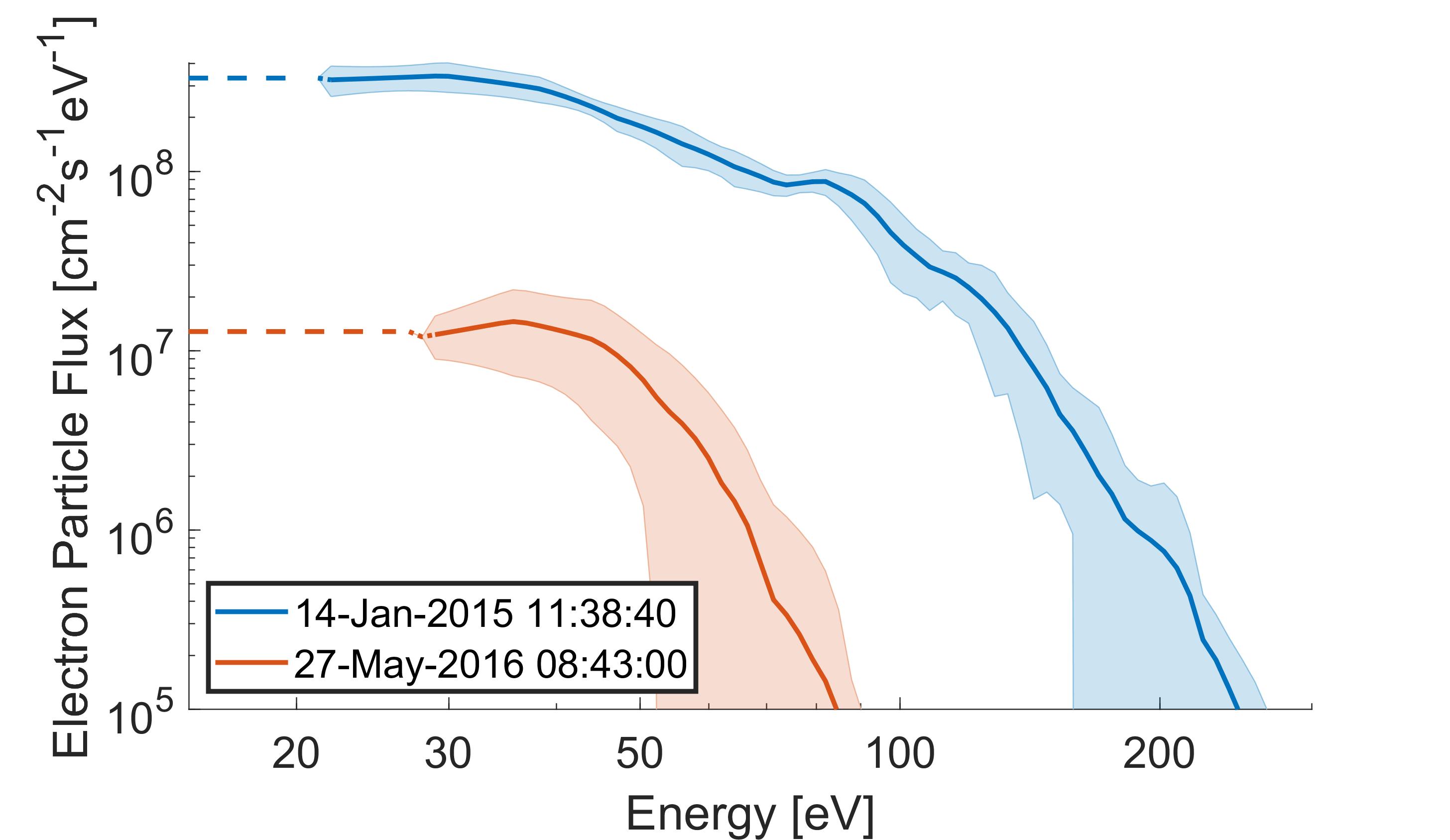
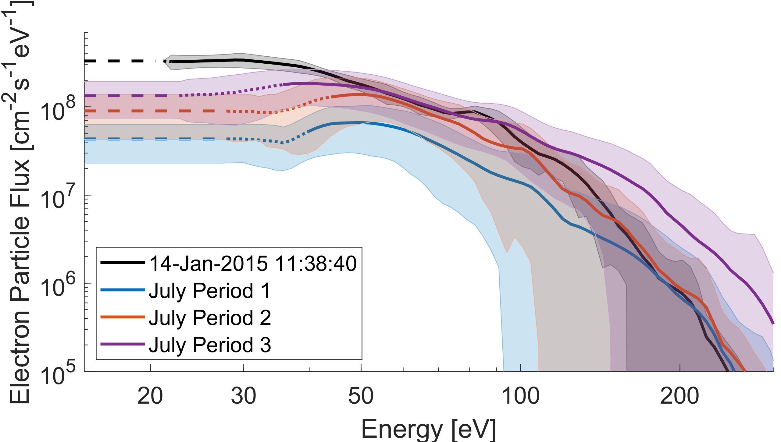
Within the duration of each FUV scan, there were several measurements of the electron flux by RPC/IES, each of which was individually corrected for the spacecraft potential at that time. The time-average and the standard deviation of the electron flux were calculated at each energy as shown in Figure 3.
Although RPC/IES could not measure the electron population below the detection threshold, there may still have been a large electron flux at low energies. As such, we extended the mean particle flux to low energies assuming a constant particle flux at low energies. We also considered extrapolating logarithmically but the method of extrapolation had little impact on the resulting emission frequency as the cross-sections decrease significantly near the threshold energies (given in Table $2$). The emission cross-sections decrease sharply near the threshold energies of each line (see Table $2$) and electrons below the threshold are unable to generate FUV emissisons. Despite large particle fluxes the low energy ($<20$ $\mathrm{eV}$) electrons contributed little to the model brightness.

Figure 3: Suprathermal electron particle flux during two nadir Alice scans during quiet periods. The solid line is the average particle flux during each of the scans, while the shaded region corresponds to the standard deviation of the electron flux in the same period. The extrapolation of the electron flux to energies below which RPC/IES could not measure, due to the spacecraft potential, is given by the dashed line.

2.5 Other sources of emission

Alongside dissociative excitation by electron impact, there are several other sources of emission that are observed at comets. We have already referred to the contribution to the Lyman series by the IPM (see Section 2.2), but this should not have been visible when viewing the surface of the nucleus from Rosetta.
We considered two main emission sources outside of electron impact: prompt-photodissociation of H2O to produce Lyman-$\beta$ and fluorescence of CO to emit in the Fourth Positive Group.
These emission features are driven by the solar flux incident on the column of gas along the line of sight. The brightness of the emissions from these sources is given by

$$B^{X,h\nu}_{l}=10^{-6}N_{l}\int\limits_{\lambda_{min}}^{\lambda_{Th}}\!\sigma_{l}^{X,h\nu}(\lambda)I(\lambda)\,\mathrm{d}\lambda,$$ (5)

where $l$ is H2O for $X=\text{Ly-$\beta$}$ and CO for $X=\text{CO4PG}$ (contributing to the CI1657 emissions).
The photon flux, $I(\lambda)$, at comet 67P was driven by TIMED-SEE (Woods et al. 2005) measurements at 1 $\mathrm{ua}$ taken at the same Carrington longitude as comet 67P for each time interval. The cross-section for resonance fluorescence of CO was based on the model of Lupu et al. (2007). For the prompt-photodissociation of H2O, we use the emission cross-section from Hans et al. (2015).
The modelled brightness of these photon-driven emissions are upper bounds as we assumed that the entire column of neutral gas along the line of sight was illuminated. In reality, the neutral column may have been partially shadowed near the nucleus, where the neutral number density was highest, and the emissions from fluorescence of CO and prompt-photodissociation of H2O will be overestimated.

3 Nadir analysis during quiet periods

3.1 Selected cases

Table 2: Cases selected in the southern hemisphere, with nadir viewing at large heliocentric distances. The horizontal lines separate nadir cases with high (Cases 1-8) and low (Cases 9-13) electron fluxes.

Case	Date	Start Time [UTC]	Integration Time [$\mathrm{s}$]	Cometocentric Distance [$\mathrm{km}$]	Heliocentric Distance [$\mathrm{ua}$]	Spacecraft Latitude [$\circ$]	Spacecraft Longitude [$\circ$]	Total Column Density [$10^{15}$ ${\mathrm{cm}}^{-2}$]
1	14/01/2015	11:38:40	3629	28.4	2.55	-23.4	-82.9	0.58
2	29/01/2015	18:40:49	6048	27.8	2.44	-63.8	5.4	0.27
3	30/01/2015	04:25:44	2419	27.8	2.43	-64.6	56.6	0.22
4	30/01/2015	06:34:42	2419	27.8	2.43	-64.2	-11.4	0.51
5	30/01/2015	07:17:41	1763	27.8	2.43	-64.0	-34.0	0.48
6	30/01/2015	11:32:18	2419	27.9	2.43	-62.5	-167.4	0.18
7	30/01/2015	15:25:50	2419	27.9	2.43	-60.5	71.35	0.28
8	26/04/2016	06:06:12	4452	21.2	2.9	-33.1	-107	1.88
9	29/01/2015	07:51:27	3629	27.8	2.44	-58.4	-17.1	0.75
10	21/04/2016	23:01:00	3398	30.9	2.85	-24.6	-57.7	1.24
11	21/03/2016	00:05:00	2603	12.2	2.62	-24.2	-36.8	1.43
12	14/05/2016	14:39:34	4613	9.8	3.0	-53.1	-111.7	1.13
13	27/05/2016	08:43:00	5592	7.0	3.09	-56.2	-42.3	1.32

In order to determine whether the FUV emissions over the southern hemisphere are driven primarily by electron impact, cases with a nadir viewing geometry over the shadowed nucleus are considered. By observing the shadowed nucleus, there is no contribution from the IPM to the observed Lyman-$\beta$ brightness and any contamination from solar photons reflected off the nucleus is minimised. This geometry also provides the best constraint on the neutral composition of the coma from the mass spectrometer (see Section 2.3).
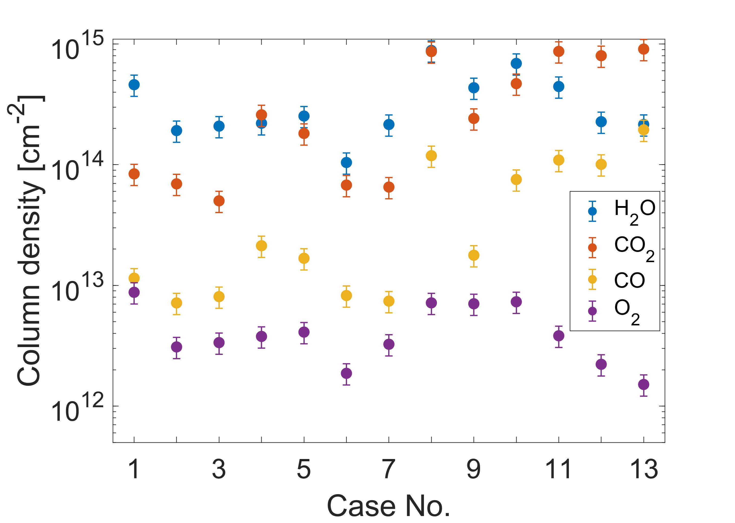
We have considered 13 cases in the southern hemisphere and at large heliocentric distances. The properties of each of these scans are outlined in Table 2. The cases have been split into two sets, which have been approached separately: nadir cases with a high suprathermal electron flux, as illustrated by the blue spectrum in Fig. 3 (Cases 1-8; Section 3.2); and nadir cases with a low suprathermal electron flux, as illustrated by the red spectrum in Fig. 3 (Cases 9-13; Section 3.3). The emission frequency for all the selected lines and the column density of each neutral species are shown in Figs. 4 and 5, respectively, for all cases in order to interpret the modelled brightnesses presented in Fig. 6, along with the FUV spectrograph observations. The average electron particle fluxes in two energy brackets are given in Table 3. The distinction between the high and low suprathermal electron flux cases (see Fig. 3) can be seen in both of the energy ranges, but to a greater extent from $60-120$ $\mathrm{eV}$.

Table 3: Average electron flux in two energy ranges for each of the nadir cases outlined in Table 2. The distinction between cases with high and low suprathermal electron fluxes is clearer in the 60-120 $\mathrm{eV}$ range.

Case	Ave. Electron Flux for $20-60$ $\mathrm{eV}$ [$10^{7}$ ${\mathrm{cm}}^{-2}\text{\,}{\mathrm{s}}^{-1}\text{\,}{\mathrm{eV}}^{-1}$]	Ave. Electron Flux for $60-120$ $\mathrm{eV}$ [$10^{7}$ ${\mathrm{cm}}^{-2}\text{\,}{\mathrm{s}}^{-1}\text{\,}{\mathrm{eV}}^{-1}$]
1	$23.2\pm 1.2$	$6.33\pm 0.85$
2	$30.4\pm 1.9$	$5.68\pm 1.34$
3	$27.7\pm 3.6$	$5.10\pm 2.62$
4	$20.5\pm 1.3$	$4.82\pm 0.95$
5	$16.9\pm 0.9$	$4.36\pm 0.65$
6	$22.2\pm 0.8$	$5.88\pm 0.56$
7	$10.5\pm 1.4$	$2.47\pm 1.01$
8	$\phantom{0}6.42\pm 0.51$	$2.60\pm 0.37$
9	$3.51\pm 0.84$	$0.05\pm 0.61$
10	$1.18\pm 0.05$	$0.22\pm 0.04$
11	$1.40\pm 0.12$	$0.06\pm 0.09$
12	$0.51\pm 0.09$	$0.01\pm 0.07$
13	$1.03\pm 0.11$	$0.03\pm 0.08$

Figure 4: Emission frequency, $v_{l}^{X}$, of each neutral species and emission line: (a) OI1356, (b) OI3014, (c) Ly-$\beta$ and OI1027, (d) CI1657 and CO4PG, and (e) CII1335. Emissions due to electron impact (e + X, Section 2.4) on CO2 (red), H2O (dark blue), CO (orange), and O2 (purple) and other processes (hν + X, Section 2.5) have been included. The uncertainty in the electron impact emission frequency is derived from the variability in the electron flux during each scan of the FUV spectrograph (see Section 2.4.2). hν + CO refers to emissions from the fluorescence of CO (green), while hν + H2O refers to the prompt-photodissociation of water (light blue) to produce Lyman-$\beta$ (see Section 2.5).

Figure 5: Column density of the four major neutral species in the coma during each of the spectrograph scans. The volume mixing ratios are derived from ROSINA/DFMS measurements (see Section 2.3).

3.2 Nadir cases 1-8

As mentioned in Section 2.3, we can derive the total neutral density in nadir viewing from in situ measurements. However, the strong dependence of the column density on the cometoradius means this method is quite uncertain. Alternatively, we can constrain the total column density by setting the modelled brightness of the OI1356 line such that it equals the observed brightness of this line. OI1356 emissions are associated with a forbidden transition (^5S - ^3P), so there are few sources of this emission line apart from electron impact. The contributions of both resonance scattering and fluorescence to this line are negligible.
There is a close agreement between the modelled and observed brightnesses for all five FUV emission lines selected for cases 1-8 (see Fig. 6). This suggests that our model represents the sources of FUV emissions in the coma well.
The emission of OI1356 is dominated by e + CO2 (red, Fig. 6a) across the high suprathermal electron flux cases. This is a result of the high emission frequency of e + CO2 ($1.08\times 10^{-8}$ ${\mathrm{s}}^{-1}$) compared to e + H2O ($4.0\times 10^{-10}$ ${\mathrm{s}}^{-1}$, see Fig. 4) in this line. The small emission frequency from e + H2O means the brightness of the OI1356 emissions is not sensitive to the column density of water. e + O2 has an OI1356 emission frequency of $5.98\times 10^{-8}$ ${\mathrm{s}}^{-1}$ in cases 1-8, larger than that from e + CO2, but the column density of O2 is insufficient for this process to contribute significantly to the total brightness (purple, Fig. 5). In case 1, e + O2 drives 0.69 R of OI1356 emission (purple, Fig. 6a), which is considerably more than the $0.1-0.2$ R of emission from this source in cases 2-8. This results from the larger column density of O2 ($8.9\times 10^{12}$ ${\mathrm{cm}}^{-2}$, Fig. 5) in case 1 than in cases 2-7 ($3.1\pm 0.9\times 10^{12}$ ${\mathrm{cm}}^{-2}$, Fig. 5), due to the more equatorial latitude compared to the southerly cases 2-7 (see Table 2). Case 8 occurred post-perihelion, when the outgassing rate of CO2 increased, resulting in a low volume mixing ratio of O2 (purple, Fig. 5), despite having a similar latitude to case 1 (see Table 2).
The OI1304 emissions are mostly driven by electron impact on CO2 and H2O (see Fig. 6b). The emission frequency of OI1304 from e + CO2 is only 1.5 times more efficient than e + H2O, in contrast to the factor of 20 in the emission frequencies of OI1356. Electron impact on CO and O2 are 1.5 and 10 times more efficient at emitting OI1304 than e + CO2 (see Fig. 4b), respectively, but the small volume mixing ratios of these molecules throughout cases 1-8 ($\ce{O2}/\ce{CO2}=0.04$; $\ce{CO}/\ce{CO2}=0.11$; Fig. 5) limits their contribution to the total OI1304 brightness. However, these processes can be a significant source of OI1304, when the volume mixing ratio of each species increases (see. Fig. 5) as seen in case 1 for e + O2 and case 8 for e + CO (see Fig. 6b).
The emission feature near 1026 $\mathrm{\SIUnitSymbolAngstrom}$ is dominated by electron impact on water throughout cases 1-8 (dark blue, Fig. 6c), generating emissions of Ly-$\beta$. As seen with OI1356 and OI1304 emissions, the largest emission frequency at this wavelength is from e + O2 at $1.17\times 10^{-8}$ ${\mathrm{s}}^{-1}$ (purple, Fig. 4c), which produces OI1027, but this is only twice that of e + H2O, so the small column density of O2 with respect to that of water means it contributes negligibly to the modelled brightness (purple, Fig. 6). Throughout these cases, we see a sizeable contribution from e + CO2 ($<0.9$ R) to the OI1027 brightness that is not seen in the northern hemisphere (Galand et al. 2020). This is especially prominent in case 8, with a post-perihelion enhanced CO2 column density of $8.66\times 10^{14}$ ${\mathrm{cm}}^{-2}$ (see Fig. 5). In cases 1-8, prompt-photodissociation of H2O (light blue, Fig. 4c) has an emission frequency 5 times smaller than from e + H2O (dark blue, Fig. 4c), so photodissociation is a minor source of emissions when the suprathermal electron flux is large (Fig. 6c). We show that e + H2O is the major source of the emissions near 1026 $\mathrm{\SIUnitSymbolAngstrom}$ in the southern hemisphere, but the contribution from e + CO2 and prompt-photodissociation of H2O to this line are not negligible.
Throughout cases 1-8, the emissions near 1657 $\mathrm{\SIUnitSymbolAngstrom}$ are dominated by CI1657 emission from electron impact on CO2 (red, Fig. 6d). There is also a small contribution from e + CO (orange, Fig. 6d) to the overlapping bands of the Fourth Positive Group, which has an emission frequency ($4.58\times 10^{-8}$ ${\mathrm{s}}^{-1}$) twice that of e + CO2 (orange and red, respectively, Fig 4d). As the suprathermal electron flux is high for these cases, fluorescence of CO (green, Fig. 4d) has a lower or similar emission frequency to e + CO2. However, the low column density of CO compared to that of CO2 (see Fig. 5) means the emissions from both electron impact on and fluorescence of CO are only minor contributions to the total brightness near 1657 $\mathrm{\SIUnitSymbolAngstrom}$ (see Fig. 6d), except in case 8, when the column density of CO ($1.19\times 10^{14}$ ${\mathrm{cm}}^{-2}$) is larger than seen in cases 1-7 (see Fig. 5).
The CII1335 emissions have significant contributions from electron impact on both CO and CO2. The emission frequency of e + CO ($2.04\times 10^{-8}$ ${\mathrm{s}}^{-1}$) is 8 times larger from e + CO2 for this line, which is balanced by a ratio of 0.11 of CO to CO2 in column density. The two competing effects result in the two species contributing approximately equally to the brightness of the CII1335 line (see Fig. 6e). This emission line is primarily driven by $60-120$ $\mathrm{eV}$ electrons due to the high threshold energies of e + CO (33 $\mathrm{eV}$) and e + CO2 (44eV, Table $2$) for this process. The electrons in this energy range vary little across cases 1-8 (see Table 3), which is reflected in the roughly constant emission frequency (see Fig. 4e). Therefore, the variations in the CII1335 brightness in cases 1-8 are driven by changes in the column densities of CO and CO2 (see Fig. 5). The large emission frequency of e + CO relative to e + CO2 (see Fig. 4e) in this line means the observed brightness is highly sensitive to the column density of CO. The volume mixing ratio of CO, derived from measurements by the mass spectrometer, includes a significant correction for fragmentation of CO2 within the instrument, which leads to a contribution to the CO signal (Dhooghe et al. 2014). The close agreement between the modelled and observed brightness of this line across cases 1-8 (Fig. 6e) suggests that the corrected $\ce{CO}/\ce{CO2}$ volume mixing ratio derived from the mass spectrometer measurements is accurate.

Figure 6: Comparison of the total modelled (black) and observed brightness (magenta), $B^{X}$, of each emission line. The stacked bars show the contribution from each neutral species and emission process. The same colour code as Fig. 4 is used. The error on the observed brightness is derived from the integration of the FUV spectra. The error on the modelled brightness is from the temporal variation of the electron flux and column density, as well as a 20% uncertainty in the neutral composition. In cases 1-8, where the observed OI1356 brightness is used to fit the total neutral column density (see Section 3.2), the error on the modelled OI1356 brightness is included in the error of the other modelled emission brightnesses.

3.3 Nadir cases 9-13

In cases 9-13, the suprathermal electron flux was very low (see Table 3) in both energy ranges. The electron flux was on average 11.8 times greater for cases 1-8 than for cases 9-13 between 20 and 60 $\mathrm{eV}$, whereas in the range $60-120$ $\mathrm{eV}$ the average flux ratio was $\sim\!{60}$. The FUV emission lines considered, except CII1335, are driven primarily by electrons from $20-60$ $\mathrm{eV}$ so the emission frequencies are a factor of $\sim\!20$ smaller in cases 9-13 than in cases 1-8 (e.g. 26.6 for Ly-$\beta$ from e + H2O; dark blue, Fig. 4c). The threshold energies for emission of CII1335 from electron impact on CO (33 $\mathrm{eV}$, see Table $2$) and CO2 (44 $\mathrm{eV}$) are much higher than for the other wavelengths considered, and hence the emissions are more dependent on the electron flux between 60 and 120 $\mathrm{eV}$. This results in a ratio of $\sim\!{50}$ in the emission frequency of the process e + CO2 (red, Fig. 4e) between the high and low flux cases.
Throughout the low flux cases, we observe no substantial emissions of OI1356 due to the low electron impact emission frequencies (see Fig. 6a). As a result, we use the radial column density, derived from the in situ pressure gauge measurements (see Section 2.3), to calculate the modelled emission brightnesses. The radial column density is calculated assuming a constant neutral gas velocity, which may result in an underestimate of the column density.
We also observe negligible emissions of OI1304 throughout this time (see Fig. 6b). The column densities in cases 9-13 are similar to cases 1-8 (see Fig. 5), so the lack of oxygen line emissions is a result of the lower electron flux (Table 3). In addition, there are negligible emissions of CII1335 (see Fig. 6e), as there are few $60-120$ $\mathrm{eV}$ electrons in the coma (Table 3). The lack of observed OI1356, OI1304, and CII1335 emissions (see Figs. 6a, 6b and  6e) in these lines is replicated in the modelled brightnesses for the cases associated with a low suprathermal electron flux. This demonstrates that the only source of these emission lines in nadir viewing is dissociative excitation by electron impact.
As shown in Fig.  6d, there are significant emissions near 1657 $\mathrm{\SIUnitSymbolAngstrom}$ for these cases, despite the small populations of energetic electrons in the coma (Table 3) and the low emission frequency of the processes e + CO ($3.96\times 10^{-9}$ ${\mathrm{s}}^{-1}$) and e + CO2 ($1.07\times 10^{-9}$ ${\mathrm{s}}^{-1}$, see Fig. 4d). The emission frequency of fluorescence of CO is $1.86\times 10^{-8}$ ${\mathrm{s}}^{-1}$ through cases 9-13, and hence is the dominant source of emissions at this wavelength. The dominance of CO fluorescence, compared to case 8, results only from the decrease in the electron impact emission frequency, as both the volume mixing ratio $\ce{CO}/\ce{CO2}=0.14\pm 0.05$ and the emission frequency from CO fluorescence (green, Fig. 6d) are similar to those in case 8. In cases 1-7, the total column density and the CO column density are on average a factor 3 times smaller than in cases 9-13, which result in a small absolute contribution from CO fluorescence (0.27 R). There is some uncertainty in the source of the CO4PG emissions in the low flux cases, as the Cameron bands, which are seen at long wavelengths, indicate that there may be emissions from CO in the 4PG driven by a large flux of low energy ($\sim$10 eV) electrons. However, we have not seen evidence of this in the measured electron flux as the spacecraft potential ($-23$ to $-17$ eV, as measured by RPC/LAP) prevented measurements at such low electron energies. Other emission lines are unaffected by these low energy electrons as these lines have a much higher threshold energy ($>$15 eV) compared to 4PG emissions from CO (8 eV, see Table $2$). Despite this, the modelled CI1657 and CO4PG emissions well represent the observed emissions in these cases, given the uncertainty in the column density, and dissociative excitation by electron impact is not the major source of emissions when the suprathermal electron flux is small.
In cases 9-13, the emission frequency of Ly-$\beta$ and OI1027 from electron impact on all species drops below the emission frequency of prompt-photodissociation of H2O ($8.6\times 10^{-10}$ ${\mathrm{s}}^{-1}$, Fig. 4c). In these cases, prompt-photodissociation of H2O is the dominant source of emissions as the process e + H2O has an emission frequency a factor four smaller ($1.97\times 10^{-10}$ ${\mathrm{s}}^{-1}$, Fig. 4c). Photodissociation of H2O is comparable in efficiency to electron impact on O2 near 1026 $\mathrm{\SIUnitSymbolAngstrom}$ but throughout these cases the number density ratio of $\ce{O2}/\ce{H2O}$ is less than $0.02$, so the contribution from electron impacts on O2 is small.
The observed and modelled brightnesses of Ly-$\beta$ and OI1027 agree closely in cases 9 and 10 but for cases 11-13 the modelled brightness is smaller than that observed (see Fig. 6c). The unexplained intense Lyman-$\beta$ emissions are unlikely to be from electron impact emissions which would produce strong signals in the other atomic lines, such as OI1304 from e + H2O at a factor $\sim 2.9$ smaller than the Ly-$\beta$ brightness.
The Lyman-$\alpha$/Lyman-$\beta$ ratio can be used as an indicator of key emission processes, with a ratio of 8 expected from pure e + H2O (Makarov et al. 2004). On 29 Nov 2014, a spectrum of pure e + H2O (Galand et al. 2020) was observed with a ratio Lyman-$\alpha$/Lyman-$\beta=4.4$. The disparity between the observed ratio and the theoretical ratio may be a result of the difficult calibration of Alice around Lyman-$\alpha$, variation in the shape of the Lyman series cross-sections or differences in the cascade emissions. Case 8, also in early 2016, has a ratio of 2.56 with a large electron flux, but the 1027Å line brightness has a large contribution of OI emissions from e + CO2. The modelled Ly-$\beta$ emissions from e + H2O in case 8 are a factor 4.4 smaller than the Ly-$\alpha$ brightness, consistent with the line ratio in Nov 2014.
Cases 11-13 have Ly-$\alpha$/Ly-$\beta=$ 2.6, 3.2 and 3.3 respectively, suggesting that a process with a small line ratio has contributed significantly to the Ly-$\beta$ brightness. Electron impact on other neutral species cannot be a strong source of OI1027 in these cases, as they would show stronger emissions in other lines (e.g. OI1356 for O2 and CO2) which were not observed. Resonant scattering of solar flux on atomic hydrogen would generate Ly-$\alpha$ emissions 300 times brighter than Ly-$\beta$, greatly increasing the line ratio. It is also very unlikely at the low cometocentric distances ($\sim 10$ km) as neutral molecules are advected away from the nucleus (timescale of the order of seconds; Galand et al. 2016) before they can undergo photodissociation (timescale $>10^{5}$ s; Huebner & Mukherjee 2015).
Prompt-photodissociation, which gives a Ly-$\alpha$/Ly-$\beta$ ratio of 1.4 (Hans et al. 2015), could generate the lower line ratio. The emission of OI1304 from this process is also very weak, as a spin forbidden transition would be required (Wu & Judge 1988). However, if we had significantly underestimated the efficiency of this process in the model, a discrepancy would be seen in the other cases. A large increase in the column of water in cases 11-13 (by a factor of 8, 15 and 5, respectively) would bring the modelled Ly-$\beta$ into agreement with the observed brightnesses, whilst generating few emissions in the other atomic lines due to the low emission frequencies (dark blue, Figs. 4a & b). However, this would result in a neutral column comprising 80% water in cases 11 and 12 (50% in case 13), which is inconsistent with the concurrent mass spectrometer measurements (see Fig 5).The required mixing ratio would also be incongruous with wider outgassing trends, as the outgassing rate of CO2 in the southern hemisphere was larger than that of H2O in Mar 2016 (Case 11) and was dominant over the outgassing of H2O near the end of mission (Cases 12 and 13; Gasc et al. 2017a; Läuter et al. 2018). The source of the Lyman-$\beta$ emissions in cases 11-13 remains unclear.

4 Corotating interaction regions in summer 2016

4.1 Selection of cases

Having confirmed that the impact of suprathermal electrons on cometary neutrals is a major source of emissions during quiet periods in the southern hemisphere in Section 3, we apply the multi-instrument analysis to the CIRs observed in the summer of 2016. The CIR was observed over four solar rotations throughout the summer of 2016 (Hajra et al. 2018), from the start of June until the beginning of September. In the present study, we consider two occurrences: one over the 9 and 10 July, and one on the 4 August. Enhanced FUV emissions were observed on two additional solar rotations in early and late September. However, observations in the FUV occurred infrequently during these events, so we could not study the temporal variability of the emissions.
During these events, the suprathermal electron flux can vary by a factor of 100 within several hours, as seen during the first periods on 4 Aug and 9 July (see Tables $3$ and 5 and Fig. 8). The brightness of the FUV emission lines are also seen to vary by a factor of ten within the same time periods (see Figs. 9 and 11). This scale of variation in the emission brightness has also been observed by Galand et al. (2020) during a solar event in October 2014 and Noonan et al. (2018) during a CME in summer 2015. To capture the variability, we use the highest temporal resolution available for both the measurements of the electron flux and the observed FUV brightness (10 $\mathrm{min}$). The emission frequencies are calculated from individual electron flux measurements, once the flux has been corrected for the spacecraft potential (see Section 2.4.2). The modelled brightness is plotted in Figures 9 and 11 at the time resolution of the electron spectrometer. We do not co-add consecutive spectra from the FUV spectrograph, as in Section 2.2, but instead evaluate the brightness at three distinct regions of the viewing slit for each spectrum. The black vertical lines are therefore indicative of the spatial variability of the emissions along the Alice slit. In Figures 9 and 11, the three regions associated with rows 8-11, 13-16, and 18-21 are given by the red, black, and blue crosses, respectively. The measurements taken simultaneously in the 3 regions of the FUV spectrograph slit are linked by vertical black lines.
Neither the case in July nor the one in August 2016 had a nadir viewing geometry as was used in Section 3. On 4 August 2016, the FUV spectrograph was viewing off the limb of the nucleus, whereas on the 9-10 July 2016 the spectrograph was pointed at the nucleus but off-nadir. In both situations it is not possible to derive the column density along the line of sight from the ROSINA in-situ measurements as was done in cases 1-8 in Section 3.2. Variation across the nucleus’ surface in both the density and composition of the outgassing neutrals means we cannot extrapolate from in situ measurements to calculate the column density along the line of sight. For the August case, the column densities of CO2 and H2O are derived from remote observations by VIRTIS-H and MIRO spectrometers, respectively, (see Section 2.3) over each of the intervals of FUV observations.
In the July event, the surface of the nucleus was illuminated, which prevents the estimation of reliable column densities using either of the spectrometers. We, therefore, set the column density of CO2 during each interval such that the scale of the modelled and observed brightnesses of the OI1356 within each interval agree, which is consistent with the approach in cases 1-8 in Section 3.2.
The column density, taken constant with each interval during the CIR events considered are given in Tables $3$ and 5. The different periods, with distinct neutral column densities, are indicated by different coloured lines in Figures 9 and 11. During each interval the nucleus moved slowly within the field of view of the spectrograph, justifying the constant column density during each interval. However, between these periods the spacecraft underwent manoeuvres in which the region of the coma observed changed rapidly, which justifies the variation of the column density from one interval to the next. As the column density is taken as constant in each interval, the variation of the modelled brightness during the time periods is only due to the fluctuations of the measured suprathermal electron flux. The average electron fluxes in each period of the FUV spectra are shown in Figures 8 and 10 for August and July, respectively. The electron flux in period 1 of the August case is split into two parts, comprising the peaks (dark blue) and troughs (light blue) of the electron flux as seen in the modelled brightness in Fig.9 (dark blue).

4.2 4 August 2016

4.2.1 Overview

Figure 7: OSIRIS WAC image (Keller et al. 2007) from 4 Aug 2016 02:00 UT during period 1 (see Section 4.2.3) with the Alice viewing slit shown in white. The line of sight passes within $\sim 500$ m of the comet nucleus.

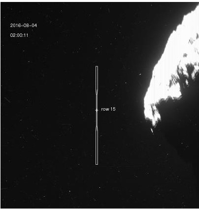
On this day the viewing geometry was limb (Fig 7), so we have used column density measurements from the VIRTIS-H and MIRO spectrometers (see Section 2.3). The column density measurements taken in the four time periods are outlined in Table 5. This solar event occurred near the end of mission at 3.5 $\mathrm{ua}$, when CO2 was dominant over H2O in the southern hemisphere as seen in Table $3$, which is consistent with a volume mixing ratio of $\ce{H2O}/\ce{CO2}\sim 0.05$ from Läuter et al. (2018). During period 2, the line of sight of the spectrograph passed over the neck region of the comet, which had an increased abundance of water (Migliorini et al. 2016), resulting in the enhanced water column density. CO was not detected during any of the four periods and the 3$\sigma$ upper-limits of the column density derived from the sub-mm spectrometer are given in Table $3$. The FUV emission spectra display weak CO band emissions which indicates there is some CO in the coma, although insufficient to be detected by MIRO. In Figure 9, we have assumed that there is no CO present in the coma as we do not have a good constraint on the CO mixing ratio throughout the column. The spectrometers could not measure the column density of O2, so we have assumed there is no O2 present in the column along the line of sight. Towards the end of mission, the mixing ratio $\ce{O2}/\ce{CO2}$ decreased ($<1$%, Läuter et al. 2018) and O2 was less abundant in the southern hemisphere (Hässig et al. 2015), so we would not expect significant emissions from e + O2. Including a few percent of O2 relative to the H2O column density has negligible impact on the emission brightness, as emissions of the atomic oxygen lines are dominated by electron impact on CO2.

Table 4: Properties of the four intervals on 4 Aug 2016 at 3.5 $\mathrm{ua}$. The first period has been split into the peaks and troughs in the electron flux, which can be seen in Fig. 9. These are the same periods as shown in Fig. 8 in dark blue (peaks) and light blue (troughs).

Period	Start Time [UTC]	End Time [UTC]	CO2 Column Density [$10^{14}$ ${\mathrm{cm}}^{-2}$]	H2O Column Density [$10^{14}$ ${\mathrm{cm}}^{-2}$]	CO Column Density [$10^{14}$ ${\mathrm{cm}}^{-2}$]	Ave. Electron Flux for 20 - 60 $\mathrm{eV}$ [$10^{7}$  ${\mathrm{cm}}^{-2}\text{\,}{\mathrm{s}}^{-1}\text{\,}{\mathrm{eV}}^{-1}$]
1 - Peaks	01:38:59	05:42:30	$6.21\pm 0.16$	$0.5\pm 0.03$	¡1.1	15.5 - 44.9
1 - Troughs						0.56 - 10.1
2	07:25:24	10:59:15	$2.65\pm 0.17$	$2.24\pm 0.09$	–	0.77 - 23.3
3	11:51:51	15:56:18	$8.43\pm 0.14$	$0.36\pm 0.02$	¡1.3	3.16 - 20.4
4	17:38:16	21:12:03	$7.93\pm 0.23$	$0.31\pm 0.02$	–	3.48 - 7.95

Figure 8: Average electron particle flux during the three periods listed in Table $3$, with the standard deviation of the flux shown by the shaded regions. The colour of each period is the same as in Fig. 9. The first period has been split into the peaks (dark blue) and troughs (light blue) in the electron flux to highlight the variability in this period. The dotted lines indicate energies where some of the RPC/IES measurements during the period could not probe, due to a high spacecraft potential (see Section 2.4.2). The dashed lines denote energies that could not be probed by any of the RPC/IES scans during the period. The electron flux from Case 1 in the nadir study (see Section 3 & Fig. 3) is plotted for comparison (black).

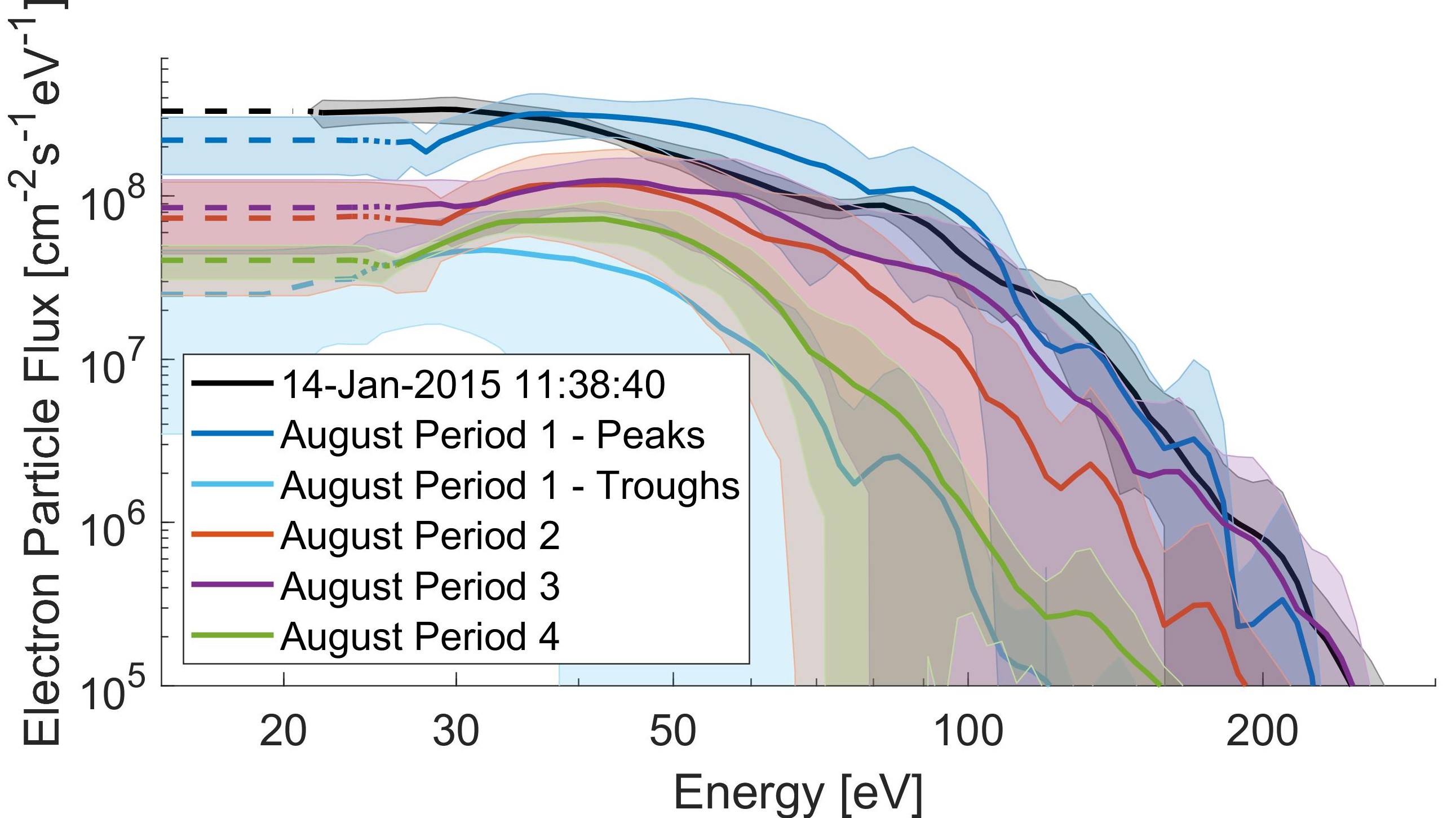
During the CIR, the variation in the suprathermal electron flux is mirrored in the brightness of the emissions in all four of the selected lines: OI1356 (Fig. 9a), CI1657 and CO4PG (Fig. 9b), Ly-$\beta$ and OI1027 (Fig. 9c), and OI1304 (Fig. 9d). This suggests that all of these emissions are strongly driven by electron impact on cometary neutrals. For limb viewing, the emissions originate from a distant region of the coma, which cannot be probed in situ. The observed correlation between the in situ measurements of the electron flux and the remote measurements of the FUV spectrograph suggest that the variations in the electron flux occur on large scales. The electron fluxes during each period (see Fig. 8) peak at 40-50 eV, which is not seen in the electron spectra during the nadir cases in quiet periods (see Fig. 3). This may result from the higher density and more energetic solar wind electrons entering the coma that are associated with the CIR.

Figure 9: Comparison of the observed (crosses) and modelled (coloured lines) brightness of four emission features, OI1356 (a), CI1657 and CO4PG (b), Lyman-$\beta$ and OI1027 (c) and OI1304 (d), during four time periods, during which a CIR was observed at comet 67P, on 4 Aug 2016 (see Table $3$). The observed brightnesses are from three regions of the FUV spectrograph slit (Rows 8-11 [red], 13-16 [black] and 18-21 [blue]). Vertical black lines link simultaneous measurements of the brightness.

4.2.2 Periods 2-4

The modelled brightness of the OI1356 emissions closely replicate both the variations and the magnitude of the observed emissions in periods 2-4 (see Fig. 9a). The emissions are dominated by e + CO2, which accounts for 98% of the modelled emissions. This is consistent with our findings from the nadir cases over the southern hemisphere (see Fig. 6a) for which the neutral composition was derived from the mass spectrometer (see Section 3.2). The close agreement in periods 2-4 suggests that there are no other significant sources of OI1356 in these cases. The lower OI1356 brightness during the second time period is a result of the lower column of CO2 compared to the following period (see Table $3$). In period 3, the OI1356 emission frequency from e + CO2 increases from $7.1\times 10^{-10}$ ${\mathrm{s}}^{-1}$ at 12:35 UT to $2.1\times 10^{-8}$ ${\mathrm{s}}^{-1}$ at 15:42UT, which causes the concurrent rise in the OI1356 brightness.
Period 4 has fewer emissions due to the small electron flux (green, Fig. 8 & Table $3$), which results in a lower emission frequency. In period 3 the emission frequency of OI1356 from e + CO2 reached $2.1\times 10^{-8}$ s^-1, five times the peak frequency in period 4 ($3.9\times 10^{-9}$ s^-1).
When looking nadir in Section 3.1, the CI1657 emissions were dominated by electron impact on CO2, with only a small contribution from fluorescence of CO (dark green, Fig. 6d) when the suprathermal electron flux was high. For limb viewing, the modelled brightness of CI1657, driven only by electron impact on CO2 (without any contribution from fluorescence of CO), well reproduces the observed brightness throughout the periods 2 and 3 (see Fig. 9b), which is consistent with there being no significant column of CO present along the line of sight ($\ce{CO}/\ce{CO2}<0.05$). Furthermore, we would not expect any significant contribution from fluorescence in this case, as e + CO is a more efficient source of emissions when the suprathermal electron flux is large (see cases 1-8, Fig. 4). In period 4, a slight underestimation of CI1657 by the model may result from the lack of CO column included in the model. A $\ce{CO}/\ce{CO2}$ ratio of 0.2 would explain the disparity, which is only slightly larger than the ratio in production rates ($\ce{CO}/\ce{CO2}=0.1$) in the southern hemisphere at this time (Läuter et al. 2018).
For limb viewing, emissions from the IPM contribute to the observed Ly-$\beta$ brightness, unlike in the nadir case (see Section 2.2). As such we include a 2-rayleigh background contribution from the IPM in this line. The Ly-$\beta$ brightness exhibits the same variations as measured in the electron flux throughout the CIR (see Fig. 9c), suggesting that dissociative excitation by electron impact is a significant source of this line.
The brightness of Ly-$\beta$ emissions is well captured throughout periods 2-4, which suggests there are no other major sources of emissions. The contribution from prompt-photodissociation of H2O to the total brightness is negligible throughout the CIR. In the limb viewing geometry, the extended coma is also observed, in which photodissociation is a significant source of neutral atoms. There could be some contribution from resonant scattering off atomic hydrogen in the extended coma, but the agreement between the modelled and observed brightnesses in Fig. 9b suggests there are not significant emissions from this source. However, it is difficult to estimate it independently as there is no constraint on the column of atomic hydrogen from remote instrumentation on Rosetta.
Again, the fluctuations of the OI1304 emission brightness mirror the changes in the suprathermal electron flux (see Fig. 9d), indicating that e + X is a major source of emission. In the nadir cases, these emissions were driven by electron impact on both CO2 and H2O (see Fig. 6b) and when the suprathermal electron flux was low there were no emissions in this line (see cases 10-14, Fig. 6). When looking at the limb, we observe substantial emissions ($\sim\!3$ R) of OI1304 when the average electron flux from $20-60$ $\mathrm{eV}$ is less than $10^{7}$ ${\mathrm{cm}}^{-2}\text{\,}{\mathrm{s}}^{-1}\text{\,}{\mathrm{eV}}^{-1}$. The disparity between the observed and modelled emissions in Fig. 9d is approximately constant throughout periods 2-4, suggesting that the residual emissions are not driven by electrons which showed strong fluctuations over the same time period. Similar to Ly-$\beta$, there may be a contribution from resonant scattering from atomic oxygen along the line of sight, but with a lack of constraints we cannot determine whether this is sufficient to explain the discrepancy.

4.2.3 Period 1

During the first period on 4 Aug 2016, the variations in the electron flux with time are mirrored by the changes in the line brightnesses for all four atomic lines. There are two strong peaks in the electron flux (dark blue, Fig. 8) from 01:45-02:20 UT and 02:40-03:40 UT during which all four of the atomic lines considered also exhibit peaks in the brightnesses. From 03:40 UT until 05:20 UT, the electron flux is small (light blue, Fig. 8) and no significant FUV emissions are observed in the atomic lines. The 2 rayleighs of Ly-$\beta$ emissions observed during this trough are attributed wholly to interplanetary emissions that are seen with a limb viewing geometry. An increase in the electron flux at the end of the first period (after 05:20 UT) also coincides with a rise in the brightnesses of the atomic lines.
However, the scale of the fluctuations related to the two strong peaks in the modelled emissions greatly exceeds those observed with the FUV spectrograph. This disparity in scale could be attributed to either a poorly estimated column density or in the electron flux along the line of sight. A reduction of the CO2 column, which was the dominant emission source in period 1, by a factor of 0.4 gives a close agreement between the modelled and observed brightnesses for all four of the atomic lines. With this reduction, there is a slight underestimation of the OI1304 brightness, which is consistent with the results in the later periods. Variation of the CO2 column density within the first period could drive the difference in scale, so we have considered higher time resolution VIRTIS data, which splits the first period into four parts. A slightly lower CO2 column is found during the first peak ($3.37\times 10^{14}$ cm^-2, 01:40-02:40 UT), but during the second peak the CO2 column density is found to be larger ($7.4\times 10^{14}$ cm^-2, 02:40-03:40 UT). The result of using these column is plotted with a dashed blue line in Figure 9.
Alternatively, the assumption that the suprathermal electron flux is constant along the line of sight may break down when viewing the extended coma. The electron flux is measured at a cometocentric distance of 12 km, but the limb observed passes within roughly 500 m of the nucleus surface at the closest point (see Fig. 7) so there could be some variation along the line of sight. Using the higher time resolution CO2 columns from VIRTIS, the electron flux would have to be reduced by a factor 0.6 during the first peak and 0.3 during the second peak to reach a close agreement between the observed and modelled brightnesses. However, if this assumption were invalid, a similar disparity to that seen in period 1 would be expected in periods 2-4, which is not the case. The viewing geometry has been compared between period 1 and periods 2-4 and there is no obvious distinction (all four periods have a line of sight passing within 1 km of the nucleus) that would cause a difference in the electron behaviour.
As the temporal variations of the electron flux and the FUV emissions are well correlated for all four atomic lines, these emissions are driven by electron impact and generated by the variations in the CIR. However, it is not clear why the brightness of the emission lines during the two large peaks in period 1 are overestimated in the model.

4.3 9 - 10 July 2016

During the CIR on 9-10 July 2016, the FUV spectrograph is viewing the illuminated nucleus, which pollutes the FUV emission spectra at long wavelengths ($>1500$ Å) and prevents reliable measurements of the column density by either spectrometer. There are only a few periods when the emissions driven by a CIR were observed by Alice, so despite the difficulties in the analysis the reflected solar photons present, this period is still of great interest.
In situ measurements do not provide a good constraint on the density and composition of the neutral gas column due to the off nadir view. Therefore, we adjust the column density during each of the periods to match the observed OI1356 emission brightness, which is consistent with our findings of CO2 driving this line over the southern hemisphere (Sections 3.2 and 4.2). The resulting column densities are given in Table 5, under the assumption of a pure CO2 coma. The adjusted column densities of CO2 are between 0.88 and 1.6 times the radial column density derived from in situ measurements of the neutral density (see Sec. 5). This is a good agreement given the variation in the outgassing across the surface and the longer path through the coma due to the viewing geometry. The off-nadir angle during periods 1-3 was roughly 10^∘, so the spatially variable outgassing is likely the major driver of the difference in column density. The in situ measurements used for this comparison have been corrected assuming the neutral gas is only CO2 (Gasc et al. 2017a).
In Figure 11, we plot only the modelled and observed brightness of the OI1356 (a) and CI1657 (b) lines, as we have no constraint on the H2O column density. The Ly-$\beta$ and OI1304 emissions both have significant contributions from e + H2O, which we cannot constrain with the OI1356 emissions (see Section 3.2).
Reflection of solar flux off the illuminated nucleus is seen in the Alice spectra at long wavelengths, strongly contributing to the atomic line at 1657 Å. In order to distinguish the CI1657 emissions from the coma from those reflected off the nucleus, we subtract the solar spectrum from the Alice observations during this event as outlined in Appendix B. OI1356 is a weak line in the solar spectrum due to the associated forbidden transition, so is unaffected by this correction. Reflected solar flux would also contribute to the Ly-$\beta$ and OI1304 brightnesses, but these lines are not considered in this section.

Table 5: Properties of the three intervals on 9-10 July.

Period	Start Time [After 9 July 2016 00:00 UTC]	End Time [After 9 July 2016 00:00 UTC]	CO2 Column Density [$10^{14}$ ${\mathrm{cm}}^{-2}$]	Total Radial Column Density [$10^{14}$ ${\mathrm{cm}}^{-2}$]	Ave. Electron Flux for 20 - 60 $\mathrm{eV}$ [$10^{7}$  ${\mathrm{cm}}^{-2}\text{\,}{\mathrm{s}}^{-1}\text{\,}{\mathrm{eV}}^{-1}$]
1	15:00:00	23:30:00	6.0	3.83	0.16 - 15.3
2	29:52:00	34:30:00	2.0	2.25	2.46 - 25.0
3	35:10:00	48:00:00	1.2	0.76	1.97 - 36.2

Figure 10: Average electron particle flux during the three periods listed in Table 5, with the standard deviation of the flux shown by the shaded regions. The colour of each period is the same as in Fig. 11. The format of the plot is the same as outlined in Figure 8.

The OI1356 brightness closely matches the variation of the electron flux during this event. Between 16:00 and 18:00 UT on 9 July, the emission frequency of OI1356 from CO2 increases from $10^{-9}$ ${\mathrm{s}}^{-1}$ at 15:45 UT, plateaus at $9\times 10^{-9}$ ${\mathrm{s}}^{-1}$ until 17:30 UT, and then drops to $4\times 10^{-10}$ ${\mathrm{s}}^{-1}$ at 17:45 UT. The close agreement in the fine structure can be seen between 07:30 and 09:30UT on 10 July. The emission frequency of OI1356 from e + CO2 increases from $5.7\times 10^{-9}$ ${\mathrm{s}}^{-1}$ to a maximum $1.3\times 10^{-8}$ ${\mathrm{s}}^{-1}$ at 08:00 UT, followed by a decrease to $1.1\times 10^{-9}$ ${\mathrm{s}}^{-1}$ at 08:40 UT. At 08:50 UT, the emission frequency and brightness of the OI1356 line both increase rapidly to $2.0\times 10^{-8}$ ${\mathrm{s}}^{-1}$ and 3.2 R, respectively, before plateauing.

Figure 11: Comparison of the observed and modelled brightness of the OI1356 (a) and CI1657 emission lines from 9 July 15:00 UT to 11 July 00:00 UT 2016. The plots follow the same format as outlined in Figure 9. The modelled brightnesses shown here are only driven by electron impact on CO2.

The observed CI1657 emissions display the same structures seen in the OI1356 brightness (e.g. between 16:00 and 18:00 UT on 9 July; Fig. 11b), capturing both the magnitude and variability of the fluctuations. On 10 July, a peak in the observed CI1657 brightness at 18:00 UT is mirrored by an increase in the CI1657 emission frequency to $5.59\times 10^{-8}$ s^-1, before a decrease in both the observed emissions from the coma and the electron flux until 21:00 UT. When there are few suprathermal electrons around 21:00 UT 10 July, there are almost no observed emissions from the coma, demonstrating that there are no other major sources of emissions from the coma during this event. The good agreement between the in situ electron measurement and remote FUV observations strengthens the case that the electron variations occur over large scales.

5 Conclusion

The Rosetta spacecraft’s proximity to the nucleus of 67P, throughout the two-year escort phase, provided us with the opportunity to observe FUV emissions from within the coma. We have performed the first forward modelling of FUV emissions in the southern hemisphere of comet 67P using an extension of the multi-instrument analysis of Galand et al. (2020) and introducing carbon lines for the first time. When observing the shadowed nucleus at large heliocentric distances, the analysis we have applied well reproduces the observed brightnesses of the selected FUV emission lines (OI1356, OI1304, Ly-$\beta$ and OI1027, CI1657 and CO4PG, and CII1335) for periods with large suprathermal electron fluxes (see Section 3.2) . Therefore, dissociative excitation by electron impact is a key source of the FUV emissions in the southern hemisphere away from perihelion. When the suprathermal electron flux was small (Averaged electron flux $<2\times 10^{7}$ ${\mathrm{cm}}^{-2}\text{\,}{\mathrm{s}}^{-1}\text{\,}{\mathrm{eV}}^{-1}$ between 20 and 60 $\mathrm{eV}$), no emission of either of the OI lines or the CII line ($B^{\text{OI1304}}<0.55$R, $B^{\text{OI1356}}<0.79$R, $B^{\text{CII1335}}<0.22$R) were observed, indicating that energetic electrons in the coma are the dominant driver of these emissions (see Section 3.3). In the low flux cases, fluorescence of CO was a larger source of emissions at 1657 Å compared to many of the cases with a high electron flux (see Fig. 6d), due to the larger total column density (see Table 2). The relative contribution of CO fluorescence in the low flux cases was also enhanced by the small emission frequency from electron impact processes (see Fig. 4d), which had dominated in the high flux cases (cases 1-8, Fig 6d).
Unlike other low suprathermal electron flux cases, in cases 11 & 12 there were significant emissions at 1027Å (5 R & 3 R), the source of which remains unclear. Electron impact on neutrals cannot be the source of the emissions as the brightness of other atomic lines, such as OI1304 and OI1356 would be significant as well. The low Lyman-$\alpha$/Lyman-$\beta$ ratios in these cases (2.6 - 3.3) rules out resonant scattering as a source (expected ratio of 300) and suggests photo-dissociation could be a driver of these emissions (expected ratio of 1.4). However, prompt-photodissociation would require significantly more H2O along the line of sight (by a factor 5-15) to generate emissions in agreement with those observed. Late in the Rosetta mission, as these cases were, water was more weakly outgassing than CO2 in the southern hemisphere (Gasc et al. 2017a; Läuter et al. 2018), so the required mixing ratios (up to 80% water) are unlikely to have occurred and are inconsistent with the in situ measurements. Therefore, the source of these unexplained Ly-$\beta$ emissions remains an open question.
In the low electron flux cases (cases 9-13), the neutral column density is derived from a very simple model (Eq. 2), where we have assumed a fixed comet radius and constant neutral gas velocity. Using a constant expansion velocity may underestimate the gas density near the nucleus by up to 50% (Heritier et al. 2017a), but this has little impact on the conclusions in these low flux cases. We have also neglected any lateral motion of the neutral gas in the coma, which could impact the composition and density of the neutrals along the line of sight. When deriving column densities from in situ measurements, a more complete 3D structure of the neutral coma (e.g. Bieler et al. 2015b), including expansion of the gas near the nucleus, could be incorporated into the multi-instrument analysis.
At large heliocentric distances, the FUV spectra obtained in the southern hemisphere are very different to those from the northern, summer hemisphere due to the prominence of CO2 in the southern hemisphere (Hässig et al. 2015), especially post perihelion (Gasc et al. 2017a). Consequently, the FUV spectra contain much stronger atomic carbon lines (CI and CII) as well as molecular bands of CO, such as the Fourth Positive Group (Feldman et al. 2018) compared to the northern hemisphere where they are barely detected. The hemispherical asymmetry in composition results in significantly different sources for several emission lines between the northern and southern hemispheres.
OI1356 is produced primarily by e + CO2 in the southern hemisphere (see Fig. 6a), whereas, in the northern hemisphere, e + O2 plays a more significant role (Galand et al. 2020). The OI1304 brightness had significant contributions from electron impact on all four of the major neutral species in the coma (CO2, H2O, CO and O2) across the selected cases over the shadowed nucleus in the southern hemisphere(see Fig. 6b). The emissions near 1026 $\mathrm{\SIUnitSymbolAngstrom}$ correspond only to emissions of Lyman-$\beta$ from e + H2O during the northern hemisphere summer (Galand et al. 2020), whereas for post-perihelion cases in the southern, winter hemisphere, there can be a significant contribution of OI1027 from e + CO2 (see case 8, Fig. 2c). Therefore, it is important to account for all four of the major neutral species when analysing FUV emission spectra over the southern hemisphere to derive column densities or mixing ratios.
The CI1657 emissions are dominated by e + CO2, when there is a large suprathermal electron flux (see Section 3.2). However when the population of suprathermal electrons in the coma is small, fluorescence of CO in the overlapping 4PG bands becomes a more significant driver of emissions near 1657 $\mathrm{\SIUnitSymbolAngstrom}$.
The brightness of the CII1335 emissions is highly sensitive to the column density of CO, due to the large emission frequency of CO compared to CO2 in this line (see Fig. 4e). The close agreement between the observed and modelled brightness of the CII1335 line confirms that the volume mixing ratio of CO derived from the ROSINA mass spectrometer is accurate, once the contribution to the CO signal due to fragmentation of CO2 in the ion source is subtracted from the CO signal on the detector (Dhooghe et al. 2014).
During the CIRs over the 9 and 10 July and on 4 August 2016, the OI1356 and CI1657 emissions were dominated by e + CO2, as attested by the agreement between the observed and modelled brightnesses (see Section 4). This is not surprising as CO2 was the dominant species outgassing from the southern hemisphere near the end of mission (Luspay-Kuti et al. 2019). For limb viewing, the Lyman-$\beta$ (Fig. 9c) and OI1304 (Fig. 9d) emissions both have significant contributions from electron impact, but the model underestimates the brightness of these lines. As the extended coma is also observed in limb viewing, resonant scattering of solar photons from atomic hydrogen and oxygen present along the line of sight may account for the discrepancy between the model and observations for these lines (Combi et al. 2004; Feldman et al. 2018). When viewing the illuminated nucleus, reflected solar flux from the nucleus introduced significant noise to the brightness of the CI1657 emissions, but the OI1356 line was generated only by dissociative excitation.
Throughout the CIRs, the brightnesses of all the selected emission lines exhibit the same temporal variation as measured in the suprathermal electron flux (Section 4). For all the time periods except the first on 4 Aug 2016, the modelled brightnesses agreed very closely with the observed line brightnesses, although there is a slight underestimation of OI1304 throughout the limb observations (see Figure 9d), which may be attributed to resonant scattering from atomic oxygen in the extended coma. Resonant scattering off atomic hydrogen may contribute to Ly-$\beta$ emissions, but this is less apparent as the emissions are much weaker than those from the IPM, which have been accounted for. It is difficult to constrain resonant scattering off atomic oxygen or hydrogen as we do not have measurements of the density of these neutrals throughout the column. The discrepancy in magnitude in the first period in August may originate from some change in the electron flux throughout the column. There should be no significant degradation of electrons in the coma at the large heliocentric distances considered (see Section 2.4.2), but a large scale potential well (Deca et al. 2017) could cause a variation of the electron flux over the extended column in limb viewing. However, if the assumption of a constant electron flux were invalid, the discrepancy should also arise in the other periods on 4 August, which have similar viewing geometries.
In a limb or off-nadir viewing geometry, the emissions originate from a distant region of the coma, which cannot be probed in situ. The observed correlation between the in situ measurements of the electron flux and the remote measurements of the FUV spectrograph suggests that any acceleration of the electron flux occurs on large scales as suggested by Deca et al. (2017). At times with low electron fluxes, such as period 4 and the troughs in period 1 on 4 August 2016, there were no strong emissions of the FUV lines, which excludes any strong local heating of electrons in a distant region along the column. These results support the findings of Galand et al. (2020) that these are solar wind electrons, which undergo acceleration by several tens of $\mathrm{eV}$ in the coma. Therefore, the FUV emissions are auroral in nature. The close correlation observed between the observed FUV auroral brightness and the electron flux allows FUV spectroscopy to be used as another measure of structures in the solar wind.
The aurora observed in the southern hemisphere of 67P is similar to the diffuse aurora at Mars in several ways. Both auroras are driven by solar wind electrons on open draped field lines (Brain et al. 2007; Volwerk et al. 2019) as shown in this study at comet 67P and by Schneider et al. (2015) at Mars. However, at comet 67P the solar wind electrons are accelerated by an ambipolar field (Deca et al. 2017, 2019), whereas at Mars the electrons driving diffuse auroras are accelerated at the Sun rather than within the Martian system (Schneider et al. 2015). Consequently, these auroras are persistent at comet 67P whereas at Mars the diffuse aurora is only observed during strong solar events.

Supporting data

All of the primary data from Rosetta used in this study will be available through ESA’s Planetary Science Archive (PSA) at www.rssd.esa.int or is available on request until posted to the archive. The processed emission line brightnesses, emission frequencies, column densities, and electron particle fluxes are made available through the Centre de Donnés astronomiques de Strasbourg (CDS) archives.

Appendix A Calculating the suprathermal electron flux from the RPC/IES counts

The Rosetta Plasma Consortium Ion and Electron Sensor (RPC/IES) was a top hat electrostatic analyser which measured the number of electron counts in bins of azimuthal angle, elevation angle and energy (Burch et al. 2007). The sensor comprised $16\times 16\times 128$ bins in these dimensions with an angular resolution of $$$\times$$$. The energy bins were distributed approximately logarithmically with a bin width $\Delta E/E=8\%$. RPC/IES measured the electron count rate in all 16 azimuthal bins simultaneously, whilst the electron and energy bins were cycled through. During the mission, anodes from the 8${}^{\text{th}}$ to 15${}^{\text{th}}$ azimuthal bins degraded (Broiles et al. 2016), hence we only used anodes 0 to 7 in our analysis.
The electron particle flux was derived from RPC/IES measurements by Heritier et al. (2018a), but here we provide an outline of each step in this calculation. Within the Level 3 files on the PSA, the background count of electrons, $C_{L3BG}$, is given for each scan of the electron spectrometer, which is independent of the instrument bin. The background count must be corrected as below before being subtracted from the counts in the measured bins.

$$C_{BG}=C_{L3BG}+\sqrt{5}C_{L3BG}$$ (6)

When installed on Rosetta, the field of view of the instrument was obscured by the main body of the spacecraft and other instruments (Clark et al. 2015). This restricted field of view has been corrected with geometric factors, $G(\theta_{0},\phi_{0},E_{0})$ (Broiles et al. 2016), where the subscript $0$ indicates that this has been evaluated on the underlying instrument grid of $16\times 16\times 128$. However, in many of the operation modes, neighbouring bins in all three dimensions were collapsed into one datapoint to reduce the demand on telemetry. Combined azimuthal bins have already been separated in the Level 2 datafiles, available on the PSA but the combined bins in elevation and energy have not been separated. We refer to $N_{bins}$, the number of combined energy bins multiplied by the number of combined elevation bins.
The counts, with background removed on the binned grid, were then un-binned onto the instrumental $16\times 16\times 128$ grid, assuming the electrons were distributed evenly between the combined bins.

$$C^{\prime}(\theta_{0},\phi_{0},E_{0},t)=\frac{C(\theta_{b},\phi_{b},E_{b},t)-C_{BG}(t)}{N_{Bins}},$$ (7)

where the subscript $b$ refers to the binned grid. The un-binned counts were then divided by the geometric factor for each bin and the integration time associated with the operation mode to convert to a differential energy flux, $g^{\prime}(\theta_{0},\phi_{0},E_{0},t)$. The geometric factor of the instrument used here is based on observations on 1 January 2015, as derived by Broiles et al. (2016).

$$g^{\prime}(\theta_{0},\phi_{0},E_{0},t)=\frac{C^{\prime}(\theta_{0},\phi_{0},E_{0},t)}{\Delta t\times G(\theta_{0},\phi_{0},E_{0})}$$ (8)

The differential flux above has not accounted for the efficiency, $\epsilon(E)$, of the MicroChannel Plates (MCPs) in the instrument, which is dependent on the impacting electron energy, E (in $\mathrm{eV}$; Kurz 1979).

$$\begin{split}\epsilon(E)=0.52&\exp\Big{(}-[\log(E+37)-2.3]^{2}/0.82\Big{)}+0.071\\ &+0.16\log(E+37)-0.028\log(E+37)^{2}\end{split}$$ (9)

We returned to the binned energy grid, $E_{b}$, by summing over combined energy bins, before dividing by the efficiency to give the differential electron particle flux (DEF), $j(\theta_{b},\phi_{b},E_{b})$.

$$j(\theta_{0},\phi_{0},E_{b},t)=\frac{\sum\limits_{\text{Comb. Energies}}g^{\prime}(\theta_{0},\phi_{0},E_{0},t)}{N_{\text{Comb. Energies}}\times\epsilon(\bar{E}_{b})\times\bar{E}_{b}},$$ (10)

where the summation is over the energy bins which were combined in the binned grid. $\bar{E_{b}}$ is the average energy of the combined energy bins. The DEF was integrated over the field of view of RPC/IES to give the electron particle flux, $J(E)$ (in ${\mathrm{cm}}^{-2}\text{\,}{\mathrm{s}}^{-1}\text{\,}{\mathrm{eV}}^{-1}$; Heritier et al. 2018a):

$$J(E_{b})=\frac{4\pi}{2\pi\sin$$}\int_{\theta_{0}=$$}^{$$}\int_{\phi_{0}=$$}^{$$}\!\cos\theta_{0}\times j(\theta_{0},\phi_{0},E_{b})\,\mathrm{d}\phi_{0}\mathrm{d}\theta_{0}$$ (11)

The term representing a geometric factor at the start of Eq. 11 is a correction for the limited field of view of RPC/IES, under the assumption of an isotropic electron particle flux at the detector.
We note that the electron particle flux at the detector was not representative of the electron flux in the coma, as the Rosetta spacecraft was generally at a spacecraft potential lower than -10 $\mathrm{V}$ (Odelstad et al. 2015). This was corrected for using Liouville’s theorem (see Eq. 4) but this prevented measurement of any electrons at low energies (see Section 2.4.2).

Appendix B Removing solar contamination from FUV emission spectra

Figure 12: Comparison of the photon flux observed by Alice at 15:58 UT 9 July 2016 to the solar photon flux, measured by TIMED-SEE at long wavelengths (1500Å - 1800 Å). Three distinct regions of the Alice slit (Rows 8-11 [red], Rows 13-16 [black] and Rows 18-21 [blue]) have been plotted which are the same as those plotted in Figure 11. The linear fits are used to scale the solar flux, so it can be subtracted from the observed Alice spectrum.

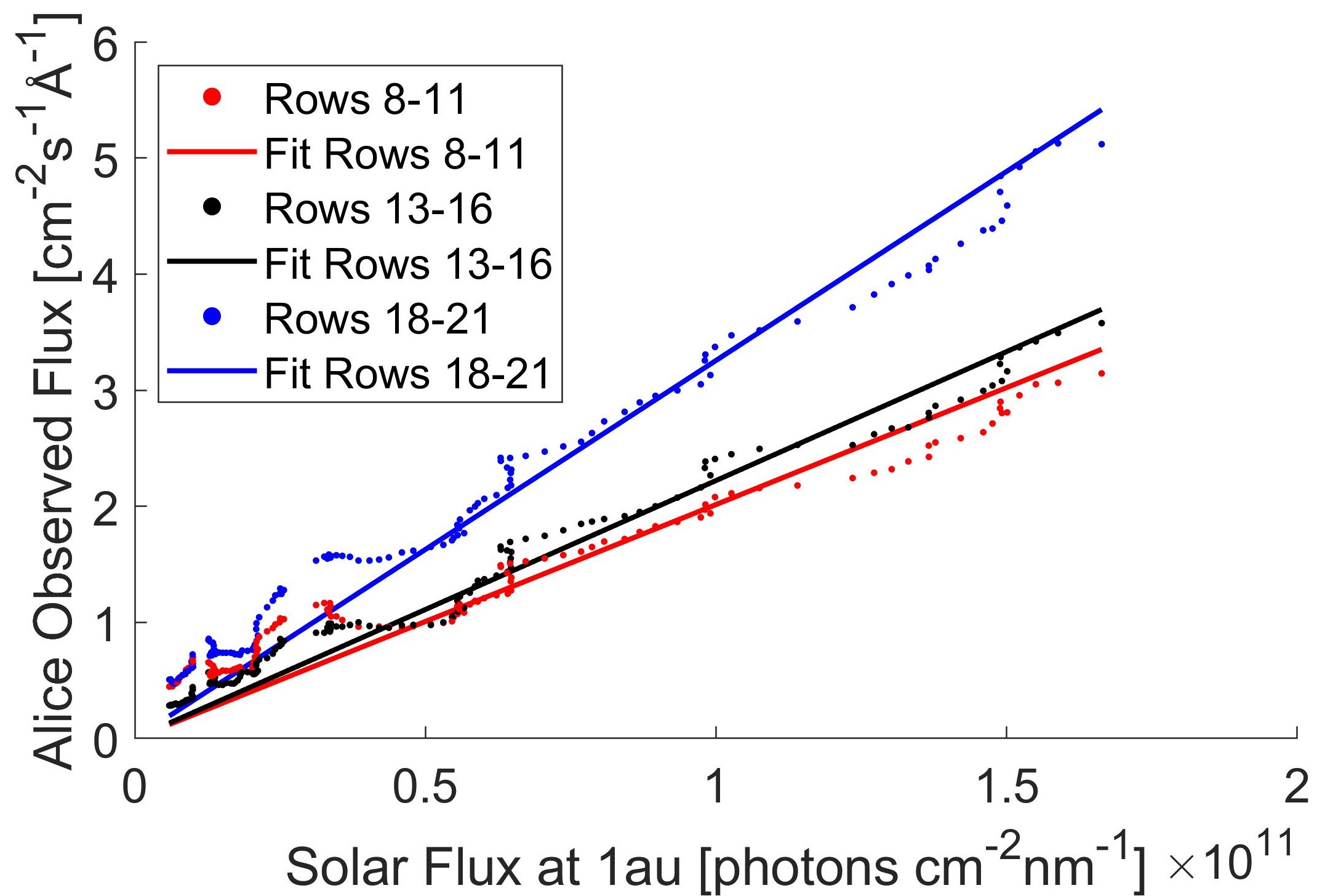
The emission spectra gathered on 9-10 July 2016 were strongly polluted by reflected solar flux from the illuminated surface of the nucleus. As we are only interested in the emissions from the coma, it was necessary to remove any contribution of reflected solar photons. The shape of the solar spectrum was taken from TIMED-SEE measurements on 16 July 2016 (green, Figure 13), which was at the same Carrington longitude as the Alice observations. As this study considers only cases at large heliocentric distances, the coma was optically thin and there should not have been significant absorption of the solar flux by cometary neutrals (Heritier et al. 2018b).

Figure 13: Breakdown of the fitting procedure to retrieve the CI1657 and CO4PG line brightness for (a) Rows 8-11, (b) Rows 13-16 and (c) Rows 18-21. The solar spectrum from TIMED-SEE (green) is smoothed and then scaled to the Alice photon flux (dark blue) at long wavelengths. The residual observed flux, once the solar spectrum is subtracted, is shown in light blue and with the CI1657 fit plotted in purple. The combination of the solar background with the CI1657 line fit is plotted in orange.

As the solar flux was more intense at the long wavelength end of the Alice spectral range (Feldman et al. 2018), the photon flux at 1au was compared to the FUV emission spectra from Alice between 1500 Å and 1800 Å for each set of co-added rows (see Figure. 12), with bright emission features around 1561 Å and 1657 Å excluded. A clear linear correlation was seen for all three regions of the Alice slit illustrating the strong presence of the solar spectrum. The reflected solar flux was derived from the linear fit (green, Fig. 13) and was subtracted from the observed Alice spectra. The residual FUV emission spectra (light blue, Fig. 13) were then fitted with a linear combination of two gaussian distributions (purple).
The CI1657 emission, measured by Alice (dark blue, Fig. 13), was more diffuse than the atomic line measured at 1au by TIMED-SEE as a result of the lower spectral resolution (8 -12 Å). The emission feature in the Alice spectra may also contain several bands of the CO Fourth Positive Group (see Section 2.2) leading to further broadening. We smoothed the TIMED-SEE flux over 10 Å to broaden the peak at 1657 Å, which better captured the width of the peak in the Alice dataset. If the adjusted goodness of fit exceeded 0.65, the line brightness is given by

$$B^{X}=(A_{1}+A_{2})\times 4\arcsin\Big{[}\sin\Big{(}\frac{\alpha}{2}\Big{)}\sin\Big{(}\frac{\beta}{2}\Big{)}\Big{]}\times\frac{10^{6}}{4\pi}$$ (12)

where the line brightness $B^{X}$ is in rayleighs and the amplitudes of the Gaussian distributions, $A_{1}$ and $A_{2}$, have units of photons cm^-2s^-1. $\alpha$ and $\beta$ are the angles subtended by the coadded rows in the Alice slit, and the numerical factor originates from the definition of 1 rayleigh (see Equation 1).

References

- Ajello (1971) Ajello, J. M. 1971, The Journal of Chemical Physics, 55, 3158
- Ajello et al. (2019) Ajello, J. M., Malone, C. P., Evans, J. S., et al. 2019, Journal of Geophysical Research (Space Physics), 124, 2954
- Balsiger et al. (2007) Balsiger, H., Altwegg, K., Bochsler, P., et al. 2007, Space Science Reviews, 128, 745
- Beegle et al. (1999) Beegle, L. W., Ajello, J. M., James, G. K., Dziczek, D., & Alvarez, M. 1999, Astronomy & Astrophysics, 347, 375
- Bieler et al. (2015a) Bieler, A., Altwegg, K., Balsiger, H., et al. 2015a, Nature, 526, 678
- Bieler et al. (2015b) Bieler, A., Altwegg, K., Balsiger, H., et al. 2015b, Astronomy & Astrophysics, 583, A7
- Biver et al. (2019) Biver, N., Bockelée-Morvan, D., Hofstadter, M., et al. 2019, A&A, 630, A19
- Biver et al. (2015) Biver, N., Hofstadter, M., Gulkis, S., et al. 2015, Astronomy & Astrophysics, 583, A3
- Bockelée-Morvan et al. (2016) Bockelée-Morvan, D., Crovisier, J., Erard, S., et al. 2016, Monthly Notices of the Royal Astronomical Society, Volume 462, Issue Suppl_1, p.S170-S183, 462, S170
- Bockelée-Morvan et al. (2015) Bockelée-Morvan, D., Debout, V., Erard, S., et al. 2015, Astronomy & Astrophysics, 583, A6
- Brain et al. (2007) Brain, D. A., Lillis, R. J., Mitchell, D. L., Halekas, J. S., & Lin, R. P. 2007, Journal of Geophysical Research (Space Physics), 112, A09201
- Broiles et al. (2016) Broiles, T. W., Livadiotis, G., Burch, J. L., et al. 2016, Journal of Geophysical Research: Space Physics, 121, 7407
- Burch et al. (2007) Burch, J. L., Goldstein, R., Cravens, T. E., et al. 2007, Space Science Reviews, 128, 697
- Bykov & Zakharov (2020) Bykov, N. Y. & Zakharov, V. V. 2020, Physics of Fluids, 32, 067109
- Carr et al. (2007) Carr, C., Cupido, E., Lee, C. G. Y., et al. 2007, ssr, 128, 629
- Chaufray et al. (2017) Chaufray, J.-Y., Bockelée-Morvan, D., Bertaux, J.-L., et al. 2017, Monthly Notices of the Royal Astronomical Society, 469, S416
- Clark et al. (2015) Clark, G., Broiles, T. W., Burch, J. L., et al. 2015, Astronomy & Astrophysics, 583, A24
- Combi et al. (2004) Combi, M. R., Harris, W. M., & Smyth, W. H. 2004, Gas dynamics and kinetics in the cometary coma: theory and observations, ed. M. C. Festou, H. U. Keller, & H. A. Weaver, 523
- Coradini et al. (2007) Coradini, A., Capaccioni, F., Drossart, P., et al. 2007, Space Science Reviews, 128, 529
- Deca et al. (2017) Deca, J., Divin, A., Henri, P., et al. 2017, Physical Review Letters, 118, 205101
- Deca et al. (2019) Deca, J., Henri, P., Divin, A., et al. 2019, Phys. Rev. Lett., 123, 055101
- Dhooghe et al. (2014) Dhooghe, F., De Keyser, J., Altwegg, K., et al. 2014, in EGU General Assembly Conference Abstracts, Vol. 16, EGU General Assembly Conference Abstracts, 6265
- Edberg et al. (2016) Edberg, N. J. T., Eriksson, A. I., Odelstad, E., et al. 2016, Journal of Geophysical Research A: Space Physics, 121, 949
- Eriksson et al. (2017) Eriksson, A. I., Engelhardt, I. A. D., André, M., et al. 2017, Astronomy & Astrophysics, 605
- Feldman et al. (2015) Feldman, P. D., A’Hearn, M., Bertaux, J.-L., et al. 2015, Astronomy & Astrophysics, 583, A8
- Feldman et al. (2018) Feldman, P. D., Weaver, H. A., A’hearn, M. F., Combi, M. R., & Russo, N. D. 2018, The Astronomical Journal, 155, 193
- Feldman et al. (2002) Feldman, P. D., Weaver, H. A., & Burgh, E. B. 2002, The Astrophysical Journal, 576, L91
- Filacchione et al. (2016) Filacchione, G., Raponi, A., Capaccioni, F., et al. 2016, Science, 354, 1563
- Fink et al. (2016) Fink, U., Doose, L., Rinaldi, G., et al. 2016, Icarus, 277, 78
- Galand & Chakrabarti (2002) Galand, M. & Chakrabarti, S. 2002, Washington DC American Geophysical Union Geophysical Monograph Series, 130, 55
- Galand et al. (2020) Galand, M., Feldman, P. D., Bockelée-Morvan, D., et al. 2020, Nature Astronomy
- Galand et al. (2016) Galand, M., Héritier, K. L., Odelstad, E., et al. 2016, Monthly Notices of the Royal Astronomical Society, 462, S331
- Gasc et al. (2017a) Gasc, S., Altwegg, K., Balsiger, H., et al. 2017a, Monthly Notices of the Royal Astronomical Society, 469, S108
- Gasc et al. (2017b) Gasc, S., Altwegg, K., Fiethe, B., et al. 2017b, Planetary and Space Science, 135, 64
- Gaskell et al. (2017) Gaskell, R., Jorda, L., Capanna, C., Hviid, S., & Gutierrez, P. 2017, SPC SHAP5 CARTESIAN PLATE MODEL FOR COMET 67P/C-G 12K PLATES, RO-C-MULTI-5-67P-SHAPE-V2.0:CG_SPC_SHAP5_012K_CART, NASA Planetary Data System and ESA Planetary Science Archive, ftp://psa.esac.esa.int
- Gilet, N. et al. (2020) Gilet, N., Henri, P., Wattieaux, G., et al. 2020, A&A, 640, A110
- Glassmeier et al. (2007) Glassmeier, K.-H., Boehnhardt, H., Koschny, D., Kührt, E., & Richter, I. 2007, Space Science Reviews, 128, 1
- Goetz et al. (2019) Goetz, C., Tsurutani, B. T., Henri, P., et al. 2019, A&A, 630, A38
- Gulkis et al. (2007) Gulkis, S., Frerking, M., Crovisier, J., et al. 2007, Space Science Reviews, 128, 561
- Hajra et al. (2018) Hajra, R., Henri, P., Myllys, M., et al. 2018, Monthly Notices of the Royal Astronomical Society, 480, 4544
- Hans et al. (2015) Hans, A., Knie, A., Schmidt, P., et al. 2015, Phys. Rev. A, 92, 032511
- Hässig et al. (2015) Hässig, M., Altwegg, K., Balsiger, H., et al. 2015, Science, 347, aaa0276
- Heinisch et al. (2019) Heinisch, P., Auster, H. U., Richter, I., & Glassmeier, K. H. 2019, A&A, 630, A46
- Heritier et al. (2017a) Heritier, K. L., Altwegg, K., Balsiger, H., et al. 2017a, Monthly Notices of the Royal Astronomical Society, 469, S427
- Heritier et al. (2018a) Heritier, K. L., Altwegg, K., Berthelier, J.-J., et al. 2018a, Nature Communications, 9, 2580
- Heritier et al. (2018b) Heritier, K. L., Galand, M., Henri, P., et al. 2018b, aap, 618, A77
- Heritier et al. (2017b) Heritier, K. L., Henri, P., Vallières, X., et al. 2017b, Monthly Notices of the Royal Astronomical Society, 469, S118
- Huebner & Mukherjee (2015) Huebner, W. & Mukherjee, J. 2015, Planetary and Space Science, 106, 11
- Itikawa (2002) Itikawa, Y. 2002, Journal of Physical and Chemical Reference Data, 31, 749
- Itikawa & Mason (2005) Itikawa, Y. & Mason, N. 2005, Journal of Physical and Chemical Reference Data, 34, 1
- James et al. (1992) James, G. K., Ajello, J. M., Kanik, I., Franklin, B., & Shemansky, D. E. 1992, Journal of Physics B Atomic Molecular Physics, 25, 1481
- Jorda et al. (2016) Jorda, L., Gaskell, R., Capanna, C., et al. 2016, Icarus, 277, 257
- Kanik et al. (1993) Kanik, I., Ajello, J. M., & James, G. K. 1993, Chemical Physics Letters, 211, 523
- Kanik et al. (2003) Kanik, I., Noren, C., Makarov, O. P., et al. 2003, Journal of Geophysical Research, 108, 5126
- Keller et al. (2007) Keller, H. U., Barbieri, C., Lamy, P., et al. 2007, Space Science Reviews, 128, 433
- Kurz (1979) Kurz, E. A. 1979, American Laboratory, 11, 67
- Lupu et al. (2007) Lupu, R. E., Feldman, P. D., Weaver, H. A., & Tozzi, G. G.-P. 2007, The Astrophysical Journal, 670, 1473
- Luspay-Kuti et al. (2019) Luspay-Kuti, A., Altwegg, K., Berthelier, J. J., et al. 2019, Astronomy & Astrophysics
- Läuter et al. (2018) Läuter, M., Kramer, T., Rubin, M., & Altwegg, K. 2018, Monthly Notices of the Royal Astronomical Society, 483, 852
- Makarov et al. (2004) Makarov, O. P., Ajello, J. M., Vattipalle, P., et al. 2004, Journal of Geophysical Research: Space Physics, 109, 1
- McConkey et al. (2008) McConkey, J. W., Malone, C. P., Johnson, P. V., et al. 2008, Physics Reports, 466, 1
- Migliorini et al. (2016) Migliorini, A., Piccioni, G., Capaccioni, F., et al. 2016, Astronomy & Astrophysics, 589, A45
- Mumma et al. (1972) Mumma, M. J., Stone, E. J., Borst, W. L., & Zipf, E. C. 1972, The Journal of Chemical Physics, 57, 68
- Noonan et al. (2018) Noonan, J. W. J., Stern, S. A., Feldman, P. D. P., et al. 2018, The Astronomical Journal, 156, 16
- Odelstad et al. (2015) Odelstad, E., Eriksson, A. I., Edberg, N. J. T., et al. 2015, Geophysical Research Letters, 42, 10,126
- Raghuram & Bhardwaj (2020) Raghuram, S. & Bhardwaj, A. 2020, Icarus, 347, 113790
- Schneider et al. (2015) Schneider, N. M., Deighan, J. I., Jain, S. K., et al. 2015, Science, 350, 0313
- Smith & Wolfe (1976) Smith, E. J. & Wolfe, J. H. 1976, Geochim. Res. Lett., 3, 137
- Stern et al. (2007) Stern, S. A., Slater, D. C., Scherrer, J., et al. 2007, Space Science Reviews, 128, 507
- Volwerk et al. (2019) Volwerk, M., Goetz, Charlotte, Behar, Etienne, et al. 2019, A&A, 630, A44
- Weaver et al. (2011) Weaver, H. A., Feldman, P. D., A’Hearn, M. F., Russo, N. D., & Stern, S. A. 2011, The Astrophysical Journal, 734, L5
- Weaver et al. (2002) Weaver, H. A., Feldman, P. D., Combi, M. R., et al. 2002, The Astrophysical Journal, 576, L95
- Wells et al. (1972) Wells, W. C., Borst, W. L., & Zipf, E. C. 1972, Journal of Geophysical Research, 77, 69
- Wells & Zipf (1974) Wells, W. C. & Zipf, E. C. 1974, Physical Review A, 9, 568
- Wilhelmi & Schartner (2000) Wilhelmi, O. & Schartner, K. H. 2000, European Physical Journal D, 11, 79
- Witasse et al. (2017) Witasse, O., Sánchez-Cano, B., Mays, M. L., et al. 2017, Journal of Geophysical Research: Space Physics, 122, 7865
- Woods et al. (2005) Woods, T. N., Eparvier, F. G., Bailey, S. M., et al. 2005, Journal of Geophysical Research, 110, A01312
- Wu & Judge (1988) Wu, C. Y. R. & Judge, D. L. 1988, The Journal of Chemical Physics, 89, 6275