Approximation Theory of Tree Tensor Networks: Tensorized Multivariate Functions

Abstract.

We study the approximation of multivariate functions with tensor networks (TNs). The main conclusion of this work is an answer to the following two questions: “What are the approximation capabilities of TNs?” and “What is an appropriate model class of functions that can be approximated with TNs?”

To answer the former: we show that TNs can (near to) optimally replicate $h$-uniform and $h$-adaptive approximation, for any smoothness order of the target function. Tensor networks thus exhibit universal expressivity w.r.t. isotropic, anisotropic and mixed smoothness spaces that is comparable with more general neural networks families such as deep rectified linear unit (ReLU) networks. Put differently, TNs have the capacity to (near to) optimally approximate many function classes – without being adapted to the particular class in question.

To answer the latter: as a candidate model class we consider approximation classes of TNs and show that these are (quasi-)Banach spaces, that many types of classical smoothness spaces are continuously embedded into said approximation classes and that TN approximation classes are themselves not embedded in any classical smoothness space.

1. Introduction

We study the approximation of real-valued functions $f:\Omega\rightarrow\mathbb{R}$ on bounded $D$-dimensional domains $\Omega\subset\mathbb{R}^{D}$. This work is a continuation of [1, 2]. We refer to [1] for a more detailed introduction.

1.1. Previous Work

Originally, TNs were used to approximate algebraic tensors $f\in\mathbb{R}^{n_{1}\times\ldots\times n_{D}}$, see, e.g., [11]. In [18], the author used tensor trains (TT) to approximate matrices by writing the row- and column-indices in the binary form $i_{\nu}=\sum_{k=1}^{L}j_{\nu}^{k}2^{k-1}$. This way a matrix can be written as a higher-order tensor

$$f(i_{1},i_{2})=\tilde{f}(j_{1}^{1},\ldots,j_{1}^{L},j_{2}^{1},\ldots,j_{2}^{L}),$$

and the higher-order tensor $\tilde{f}$ can be approximated by TTs. This was later coined the Quantics Tensor Train (QTT) [15] and morphed into Quantized TT over time. Representations of polynomials with the QTT format were studied in [8, 19] and numerical approximation for PDEs in [14] (and references therein).

In parts I and II of this work [1, 2], we studied approximation theoretic properties of TNs for one-dimensional ($D=1$) functions in various smoothness spaces. In this work, part III, we extend our results to the multi-dimensional setting $D>1$.

1.2. Approximation and Smoothness Classes

Given an approximation tool $\Phi=(\Phi_{n})_{n\geq 0}$, approximation classes of $\Phi$ are sets of functions $A^{\alpha}(\Phi)$ for which the error of best approximation

(1.1) $$E(f,\Phi_{n}):=\inf_{\varphi\in\Phi_{n}}\left\|f-\varphi\right\|,$$

decays like $n^{-\alpha}$ for $\alpha>0$. One of the most powerful results of the approximation theory of the 20th century (see, e.g., [4]) is that, if $\Phi_{n}$ are piece-wise polynomials, the classes $A^{\alpha}(\Phi)$ are in fact (quasi-) Banach spaces and are isomorph to Besov smoothness spaces. Specifically, if the error is measured in the $L^{p}(\Omega)$-norm $\left\|\cdot\right\|_{p}$, $\Phi_{n}$ is the linear span of $n$ piece-wise polynomials, and $B^{s}_{p}(L^{p}(\Omega))$ is the Besov space of regularity order $s$ – as measured in the $L^{p}$-norm – then, eq. 1.1 decays with rate $n^{-s/D}$ if and only if $f\in B^{s}_{p}(L^{p}(\Omega))$.

For the case of nonlinear (best $n$-term) approximation, one has a similar characterization but with a much weaker regularity requirement $f\in B^{s}_{\tau}(L^{\tau}(\Omega))$ where $1/\tau=s/D+1/p$. The space $B^{s}_{\tau}(L^{\tau}(\Omega))$ is said to be “on the embedding line” since functions in this spaces barely have enough regularity to be $p$-integrable. This is best depicted in the DeVore diagram in Figure 1 or the embeddings in Theorem 5.4.

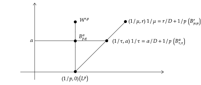
Figure 1. DeVore diagram of smoothness spaces [4]. The Sobolev embedding line is the diagonal with the points $(1/\tau,\alpha)$ and $(1/\mu,r)$

.

Such results justify the claim that piece-wise polynomial approximation, both linear and nonlinear, is mathematically fully understood. Approximation with networks, on the other hand, is not. This work is a contribution towards a better understanding of these approximation tools. We will compare TN-approximation classes with what is well-known: piece-wise polynomial approximation classes and classical smoothness spaces.

1.3. Main Results and Outline

Our results can be summarized in words as follows.

• We show that TNs can achieve the same performance (measured by eq. 1.1) for classical smoothness spaces as piece-wise polynomial approximation methods, linear or nonlinear, and of arbitrary polynomial degree. I.e., TNs can (asymptotically) optimally replicate $h$-uniform and $h$-adaptive approximation, for any smoothness order of the target function. Moreover, it is known that TNs can replicate $hp$-approximation and achieve exponential convergence for analytic functions, see, e.g., [2, 14]. Such results are comparable to some universal expressivity results for other types of deep neural networks, see, e.g., [20, 10, 9, 21, 17, 3].

• We show that for certain network topologies the approximation classes of TNs are (quasi-) Banach spaces.

• We show that Besov spaces of any order of isotropic, anisotropic or mixed smoothness are continuously embedded in TN-approximation classes.

• We show that TN-approximation classes themselves are not embedded in any Besov space.

For brevity, we consider only $\Omega=[0,1)^{D}$. However, the approximation results can be extended to any bounded Lipschitz domain $\Omega\subset\mathbb{R}^{D}$, see also Section 7.

Outline

In Section 2, we show how $L^{p}(\Omega)$ can be isometrically identified with a tensor space of any order. We define subspaces of $L^{p}(\Omega)$ which will contain our approximations. In Section 3, we briefly review tensor networks for multivariate approximation and define our approximation tool. In Section 4, we define approximation classes of tensor networks and show under which conditions these are (quasi-) Banach spaces. In Section 5, we review classical smoothness spaces and piece-wise polynomial approximation. Section 6 contains our main results. We show how spline systems can be encoded as (or approximated by) a tensor network and estimate the resulting complexity. We prove approximation rates, direct and inverse embeddings. Section 7 contains some concluding remarks.

2. Tensorization

In part I [1] of this work, we discussed in detail how one-dimensional functions can be identified with tensors or tensorized. In this section, we extend the tensorization procedure to higher dimensions. We omit details that are – more or less – the same as in the one-dimensional case. Throughout this work $b$ is some integer $b=2,3,\ldots$ and $I_{b}:=\{0,\ldots,b-1\}$.

Unlike for $D=1$, there are many valid approaches for tensorization in higher dimensions. In a rather general setting, tensorization of functions $f:\Omega\rightarrow\mathbb{R}$ over a domain $\Omega\subset\mathbb{R}^{D}$ can be performed for any domain $\Omega$ that can be encoded as $F:I_{b}^{Q}\times[0,1]^{D}\rightarrow\Omega$ via some bijective transformation $F$, with $(i_{1},\ldots,i_{Q})\in I_{b}^{Q}$ encoding some element of a partition of $\Omega$ ($Q$ bits when $b=2$). For the sake of a comprehensible presentation, we will focus on $\Omega=[0,1)^{D}$ and a very specific tensorization that is most relevant for Sections 4 and 6.

In fact, the tensorization scheme we choose is conceptually close to the one-dimensional case such that many properties are inherited with similar proof. As will become clear in Section 4, this choice of tensorization is required to ensure the approximation classes we define in Definition 4.10 are (quasi-) Banach spaces. However, the results presented in this section can be extended to more general domains and tensorizations.

2.1. The Tensorization Map

Fix a level parameter $L\in\mathbb{N}_{\geq 0}$ and define the conversion/encoding map $t^{D}_{b,L}:I_{b}^{LD}\times[0,1)^{D}\rightarrow[0,1)^{D}$ via

$$t^{D}_{b,L}(i_{1}^{1},\ldots,i_{D}^{1},\ldots,i_{1}^{L},\ldots,i_{D}^{L},\bar{x}_{1},\ldots,\bar{x}_{D})=\left(\sum_{k=1}^{L}i_{1}^{k}b^{-k}+b^{-L}\bar{x}_{1},\ldots,\sum_{k=1}^{L}i_{D}^{k}b^{-k}+b^{-L}\bar{x}_{D}\right).$$

With this we can define a tensorization map that transforms a $D$-variate function into a $(L+1)D$-variate function.

Definition 2.1 (Tensorization Map).

We define the tensorization map $T^{D}_{b,L}:\mathbb{R}^{[0,1)^{D}}\rightarrow\mathbb{R}^{I_{b}^{LD}\times[0,1)^{D}}$ as

$$(T^{D}_{b,L}f)(i_{1}^{1},\ldots,i_{D}^{L},\bar{x}_{1},\ldots,\bar{x}_{D}):=f(t^{D}_{b,L}[i_{1}^{1},\ldots,i_{D}^{L},\bar{x}_{1},\ldots,\bar{x}_{D}]).$$

Theorem 2.2 (Isometry).

Equip $[0,1)^{D}$ with the standard Lebesgue measure $\lambda^{D}$ and $I_{b}^{LD}\times[0,1)^{D}$ with the product measure $\mu_{b,L}:=\mu_{b}^{\otimes LD}\otimes\lambda^{D}$, where $\mu_{b}$ is the uniform probability measure on $I_{b}=\{0,\ldots,b-1\}$. Then, the following holds.

1. The map $T^{D}_{b,L}$ is an isomorphism between the space of (Borel) measurable functions $\mathbb{R}^{[0,1)^{D}}$ and $\mathbb{R}^{I_{b}^{LD}\times[0,1)^{D}}$.

2. The map $T^{D}_{b,L}$ is an isometry between $L^{p}([0,1)^{D})$ and the tensor space

   $$\boldsymbol{V}^{D}_{b,L}:=\ell^{p}_{\mu_{b}}(I_{b})^{\otimes LD}\otimes L^{p}([0,1))^{\otimes D},$$

   for $0<p\leq\infty$, where $\boldsymbol{V}^{D}_{b,L}$ is equipped with the (quasi-)$L^{p}$-norm associated with the measure $\mu_{b,L}$. Moreover, $\|\cdot\|_{\boldsymbol{V}^{D}_{b,L}}$ is a (quasi-)crossnorm, and, for $1\leq p\leq\infty$, it is a reasonable crossnorm.

Proof.

This follows from [1, Theorem 2.15] of part I for the case $D=1$. The results naturally extend to the case $D>1$. ∎

2.2. Finite-Dimensional Subspaces

In this work we are concerned with approximation, and thus we consider a subspace of $\boldsymbol{V}^{D}_{b,L}$ defined by

$$\boldsymbol{V}^{D}_{b,L,S^{D}}:=\mathbb{R}^{I_{b}^{LD}}\otimes S^{D},$$

where $S^{D}\subset L^{p}([0,1)^{D})$ is some finite-dimensional subspace. Since $\boldsymbol{V}^{D}_{b,L,S^{D}}$ can be identified with a subspace of $L^{p}([0,1)^{D})$ through the use of the tensorization map $T^{D}_{b,L}$, we set

$${V}^{D}_{b,L,S^{D}}:=(T^{D}_{b,L})^{-1}(\boldsymbol{V}^{D}_{b,L,S^{D}}).$$

As in part I, to ensure the approximation classes defined in Definition 4.10 are actually (quasi-) Banach spaces, it is necessary for ${V}^{D}_{b,L,S^{D}}$ to possess a hierarchical structure. Thus, we require

Definition 2.3 (Closed Under $b$-adic Dilation).

We say $S^{D}$ is closed under $b$-adic dilation if for any $f\in S^{D}$ and any $k\in\{0,\ldots,b-1\}^{D}$

$$f(b^{-1}(\cdot+k))\in S^{D}.$$

This implies

Theorem 2.4 (Hierarchy of Spaces ${V}^{D}_{b,L,S^{D}}$).

If $S^{D}\subset L^{p}([0,1)^{D})$ is closed under $b$-adic dilation, then

1. it holds

   $$S^{D}=:V_{b,0,S^{D}}\subset V_{b,1,S^{D}}\subset V_{b,2,S^{D}}\subset\ldots,$$

2. the set

   $$V^{D}_{b,S^{D}}:=\bigcup_{L=0}^{\infty}{V}^{D}_{b,L,S^{D}}$$

   is a subspace of $L^{p}([0,1)^{D})$,

3. and, if $S^{D}$ contains the constant function one, $V_{b,S^{D}}$ is dense in $L^{p}([0,1)^{D})$ for $0<p<\infty$.

Proof.

Follows with similar arguments as in [1, Theorem 2.25] of part I. ∎

In Section 6, we will employ $S^{D}:=(\mathbb{P}_{m})^{\otimes D}$, where $\mathbb{P}_{m}$ is the space of polynomials of degree $m\in\mathbb{N}_{\geq 0}$, restricted to $[0,1)$. In this case we will simply write

$$\boldsymbol{V}^{D}_{b,L,m}:=\mathbb{R}^{I_{b}^{LD}}\otimes(\mathbb{P}_{m})^{\otimes D},\quad{V}^{D}_{b,L,m}:=(T^{D}_{b,L})^{-1}(\boldsymbol{V}^{D}_{b,L,m}),\quad V_{b,m}^{D}:=\bigcup_{L=0}^{\infty}{V}^{D}_{b,L,m}.$$

3. Tensor Networks

Our approximation tool will consist of functions in $V_{b,m}^{D}$ identified (through $T_{b,L}^{D}$) with a tensor network. In this section, we briefly review some key notions about tensor networks relevant to our work. We only discuss the finite-dimensional case, i.e., for ${V}^{D}_{b,L,S^{D}}$ we consider only $\dim(S^{D})<\infty$. This greatly simplifies the presentation and is sufficient for approximation purposes, but several aspects of the theory apply to the infinite-dimensional case as well.

3.1. Ranks and Minimal Subspaces

For some fixed level $L\in\mathbb{N}_{\geq 0}$, assume $S^{D}=(S)^{\otimes D}$ for some finite-dimensional $S\subset L^{p}([0,1))$ and set

$$V_{\nu} :=\mathbb{R}^{I_{b}}, \quad\nu=1,\ldots,LD,$$

$$V_{\nu} :=S, \quad\nu=LD+1,\ldots,(L+1)D,$$

i.e., $\boldsymbol{V}^{D}_{b,L,S^{D}}=\bigotimes_{\nu=1}^{(L+1)D}V_{\nu}$. Then, we can define the notion of (multilinear) rank by identifying an order-$(L+1)D$ tensor from $\boldsymbol{V}^{D}_{b,L,S^{D}}$ with an order-2 tensor from

$$\boldsymbol{V}_{\beta}\otimes\boldsymbol{V}_{\beta^{c}},\quad\boldsymbol{V}_{\beta}:=\bigotimes_{\nu\in\beta}V_{\nu},\;\boldsymbol{V}_{\beta^{c}}:=\bigotimes_{\nu\in\beta^{c}}V_{\nu},\quad\beta\subset\{1,\ldots,(L+1)D\},\;\beta^{c}:=\{1,\ldots,(L+1)D\}\setminus\beta.$$

as follows.

Definition 3.1 ($(\beta,L)$-Rank).

The $\beta$-rank of a tensor $\boldsymbol{f}\in\boldsymbol{V}^{D}_{b,L,S^{D}}$ is defined as the smallest $r_{\beta}(\boldsymbol{f})\in\mathbb{N}_{\geq 0}$ such that

$$\boldsymbol{f}=\sum_{k=1}^{r_{\beta}(\boldsymbol{f})}\boldsymbol{v}_{\beta}^{k}\otimes\boldsymbol{w}_{\beta^{c}}^{k},\quad\boldsymbol{v}_{\beta}^{k}\in\boldsymbol{V}_{\beta},\;\boldsymbol{w}_{\beta^{c}}^{k}\in\boldsymbol{V}_{\beta^{c}}.$$

For a function $f\in L^{p}([0,1)^{D})$, the $(\beta,L)$-rank $r_{\beta,L}(f)$ of $f$ is defined as

$$r_{\beta,L}(f):=r_{\beta}(T^{D}_{b,L}(f)).$$

For $\beta=\{1,\ldots,\nu\}$, we abbreviate $r_{\{1,\ldots,\nu\}}(\boldsymbol{f})$ and $r_{\{1,\ldots,\nu\},L}(f)$ as $r_{\nu}(\boldsymbol{f})$ and $r_{\nu,L}(f)$, respectively.

For a given $\boldsymbol{f}\in\boldsymbol{V}^{D}_{b,L,S^{D}}$ not every combination of ranks is possible. In particular, we have

Lemma 3.2 (Admissible Ranks).

Let $\boldsymbol{f}\in\boldsymbol{V}^{D}_{b,L,S^{D}}$ and $\beta\subset\{1,\ldots,(L+1)D\}$ for some level $L\in\mathbb{N}_{\geq 0}$. Then, it holds $r_{\beta}(\boldsymbol{f})=r_{\beta^{c}}(\boldsymbol{f})$, and, for any partition $\beta=\gamma\cup\alpha$, it holds

$$r_{\beta}(\boldsymbol{f})\leq r_{\gamma}(\boldsymbol{f})r_{\alpha}(\boldsymbol{f}),$$

and in particular,

$$r_{\nu+1}(\boldsymbol{f}) \leq br_{\nu}(\boldsymbol{f}) \quad\quad r_{\nu}(\boldsymbol{f})\leq br_{\nu+1}(\boldsymbol{f}),\quad 1\leq\nu\leq LD-1,$$

$$r_{\nu+1}(\boldsymbol{f}) \leq\dim(S)r_{\nu}(\boldsymbol{f}) \quad\quad r_{\nu}(\boldsymbol{f})\leq\dim(S)r_{\nu+1}(\boldsymbol{f}),\quad LD\leq\nu\leq(L+1)D-1.$$

Proof.

See [1, Lemma 2.11] of part I. ∎

A concept closely related to ranks are minimal subspaces.

Definition 3.3 (Minimal Subspaces).

For $\boldsymbol{f}\in\boldsymbol{V}^{D}_{b,L,S^{D}}$ and $\beta\subset\{1,\ldots,(L+1)D\}$, the minimal subspace $\boldsymbol{U}^{\min}_{\beta}(\boldsymbol{f})$ of $\boldsymbol{f}$ is the smallest subspace $\boldsymbol{U}_{\beta}\subset\boldsymbol{V}_{\beta}$ such that $\boldsymbol{f}\in\boldsymbol{U}_{\beta}\otimes\boldsymbol{V}_{\beta^{c}}$, and its dimension is

$$\dim(\boldsymbol{U}^{\min}_{\beta}(\boldsymbol{f}))=r_{\beta}(\boldsymbol{f}).$$

For certain unfolding modes $\beta$, it is helpful to picture $\boldsymbol{U}^{\min}_{\beta}(\boldsymbol{f})$ as the space of linear combinations of partial evaluations of $\boldsymbol{f}$ (see also [1, Figure 3]).

Definition 3.4 (Partial Evaluations).

For $\boldsymbol{f}\in\boldsymbol{V}^{D}_{b,L}$, $\beta\subset\{1,\ldots,LD\}$ and any $\nu_{\beta}:=(\nu_{1},\ldots,\nu_{\#\beta})\in I_{b}^{\#\beta}$, we let $\boldsymbol{f}(\nu_{\beta},\cdot)\in\boldsymbol{V}_{\beta^{c}}$ be a partial evaluation of $\boldsymbol{f}$ (i.e., an evaluation at $\nu_{\beta}$ for the variables of modes in $\beta$). Note that we have the identity (see [1, Lemma 2.12])

$$\boldsymbol{U}^{\min}_{\beta^{c}}(\boldsymbol{f})=\operatorname*{span}\left\{\boldsymbol{f}(\nu_{\beta},\cdot):\nu_{\beta}\in I_{b}^{\#\beta}\right\}\quad\text{and}\quad\dim(\boldsymbol{U}^{\min}_{\beta}(\boldsymbol{f}))=\dim(\boldsymbol{U}^{\min}_{\beta^{c}}(\boldsymbol{f})).$$

As we saw in Definition 3.1, a function $f\in L^{p}([0,1)^{D})$ can be associated with different levels $L\in\mathbb{N}_{\geq 0}$, and, in particular, the ranks $r_{\beta,L}(f)$ may depend on the level $L$. From Theorem 2.4, we know ${V}^{D}_{b,L,S^{D}}\subset V_{b,L+1,S^{D}}\subset\ldots$. In order to guarantee this hierarchy property, the type of level extension from ${V}^{D}_{b,L,S^{D}}$ to $V_{b,L+1,S^{D}}$ as implied by Definition 2.1 is essential.

Unlike in the one-dimensional case, for $D>1$ there are many valid strategies for increasing the representation level. E.g., a natural approach would be to tensorize each of the $D$ spatial dimensions separately, leading to $D$ level parameters $(L_{1},\ldots,L_{D})$. The notion of higher/lower level may thus be, in general, not well-defined anymore since we only have a partial (inclusion) ordering on the set of tensor spaces of different levels – due to the presence of several coordinate directions. Moreover, even if the hierarchy property from Theorem 2.4 is guaranteed, for approximation with controlled complexity we need to relate the ranks of $r_{\beta,L}(f)$ for different $L$. We will return to this issue in Section 4, where we will see that a specific choice of level extension and tensor networks guarantees that the resulting approximation classes are (quasi-) Banach spaces.

3.2. Tree Tensor Networks

Let $T$ be a collection of subsets of $\{1,\ldots,(L+1)D\}$. For a rank vector $\boldsymbol{r}=(r_{\beta})_{\beta\in T}\in\mathbb{N}_{\geq 0}^{\#T}$, we define the set of tensors in $\boldsymbol{V}^{D}_{b,L,S^{D}}$ with ranks bounded by $\boldsymbol{r}$ as

$$\mathcal{T}^{T}_{\boldsymbol{r}}(\boldsymbol{V}^{D}_{b,L,S^{D}}):=\left\{\boldsymbol{f}\in\boldsymbol{V}^{D}_{b,L,S^{D}}:\;r_{\beta}(\boldsymbol{f})\leq r_{\beta},\;\beta\in T\right\}.$$

We call $\mathcal{T}^{T}_{\boldsymbol{r}}(\boldsymbol{V}^{D}_{b,L,S^{D}})$ a tree-based tensor format if $T$ is a dimension partition tree (or a subset of a dimension partition tree). In this case a tensor $\boldsymbol{f}\in\mathcal{T}^{T}_{\boldsymbol{r}}(\boldsymbol{V}^{D}_{b,L,S^{D}})$ admits a parametrization with low-order tensors and can thus be interpreted as a tree tensor network. We will work with one particular type of networks.

Definition 3.5 (Tensor Train (TT) Format).

For $T:=\left\{\{1\},\{1,2\},\ldots,\{1,\ldots,(L+1)D-1\}\right\}$ (a subset of a linear tree) and $\boldsymbol{r}=(r_{\nu})_{\nu=1}^{(L+1)D-1}$, we call

$$\mathcal{TT}_{\boldsymbol{r}}(\boldsymbol{V}^{D}_{b,L,S^{D}}):=\mathcal{T}^{\boldsymbol{T}}_{\boldsymbol{r}}(\boldsymbol{V}^{D}_{b,L,S^{D}})$$

the set of tensors in the tensor train (TT) format.

If $\{\varphi_{k}:\;1\leq k\leq\dim S\}$ is a basis of $S$, a tensor $\boldsymbol{f}\in\mathcal{TT}_{\boldsymbol{r}}(\boldsymbol{V}^{D}_{b,L,S^{D}})$ admits a representation

(3.1) $$\boldsymbol{f}(i_{1}^{1},\ldots,i_{D}^{L},\bar{x}_{1},\ldots\bar{x}_{D})=\sum_{k_{1}=1}^{r_{1}}\cdots\sum_{k_{(L+1)D}=1}^{r_{(L+1)D}}\sum_{n_{1},\ldots,n_{D}=1}^{\dim S}U_{1}(i_{1}^{1},k_{1})\cdots U_{LD}(k_{LD-1},i_{D}^{L},k_{LD})$$

$$U_{LD+1}(k_{LD},n_{1},k_{LD+1})\varphi_{n_{1}}(\bar{x}_{1})\cdots U_{(L+1)D}(k_{(L+1)D-1},n_{D})\varphi_{n_{D}}(\bar{x}_{D})$$ ,

with parameters $U_{1}\in\mathbb{R}^{b\times r_{1}}$, $U_{\nu}\in\mathbb{R}^{r_{\nu-1}\times b\times r_{\nu}}$ for $2\leq\nu\leq LD$, $U_{\nu}\in\mathbb{R}^{r_{\nu-1}\times\dim S\times r_{\nu}}$ for $LD+1\leq\nu\leq(L+1)D-1$, and $U_{(L+1)D}\in\mathbb{R}^{r_{(L+1)D-1}\times\dim S}$. The parameters

$$\boldsymbol{U}:=(U_{1},\ldots,U_{(L+1)D})\in\mathcal{P}_{b,L,S,\boldsymbol{r}}:=\mathbb{R}^{b\times r_{1}}\times\ldots\times\mathbb{R}^{r_{(L+1)D-1}\times\dim S},$$

form a tree tensor network, see Figure 2.

Figure 2. A tensor diagram corresponding to $\boldsymbol{f}=\mathcal{R}_{b,L,S,\boldsymbol{r}}(\boldsymbol{U})$.

Such tensor networks can also be associated with a recurrent sum-product neural network, where $r_{\nu}$ is the number of neurons in layer $\nu$. With eq. 3.1 we can define a representation map

$$\mathcal{R}_{b,L,S,\boldsymbol{r}}:\mathcal{P}_{b,L,S,\boldsymbol{r}}\rightarrow(T^{D}_{b,L})^{-1}\left(\mathcal{TT}_{\boldsymbol{r}}(\boldsymbol{V}^{D}_{b,L,S^{D}})\right)\subset L^{p}([0,1)^{D}).$$

The basis of our analysis of nonlinear approximation in the next section will be the following set.

Definition 3.6 (TT-Functions).

For $L\in\mathbb{N}_{\geq 0}$, a finite-dimensional space $S$ and a finite TT-rank vector $\boldsymbol{r}=(r_{\nu})_{\nu=1}^{(L+1)D-1}$, we define the set of TT-functions as

$$\Phi_{b,L,S,\boldsymbol{r}}:=\left\{\varphi=\mathcal{R}_{b,L,S,\boldsymbol{r}}(\boldsymbol{U}):\;\boldsymbol{U}\in\mathcal{P}_{b,L,S,\boldsymbol{r}}\right\}.$$

4. Approximation Classes

Approximation classes are sets of elements that can be approximated with a certain rate by a pre-specified approximation tool. It is a powerful analysis instrument for studying approximability properties of a given tool. These classes were extensively studied in the 20th century in an attempt to systematically characterize piece-wise polynomial and wavelet approximation, see [4]. In this work and in [1, 2], we apply this machinery to the study of TN-approximation. We will see that for certain classes one can derive strong statements about their properties.

4.1. Basic Notions

Let $X$ be a quasi-normed vector space and consider subsets $\Phi_{n}\subset X$ for any $n\in\mathbb{N}_{\geq 0}$. For the approximation tool $\Phi:=(\Phi_{n})_{n\in\mathbb{N}_{\geq 0}}$, define the best approximation error

$$E_{n}(f):=E(f,\Phi_{n})_{X}:=\inf_{\varphi\in\Phi_{n}}\|f-\varphi\|_{X}.$$

Definition 4.1 (Approximation Classes).

For any $f\in X$, $\alpha>0$ and $0<q\leq\infty$, define the quasi-norm

$$\left\|f\right\|_{A^{\alpha}_{q}}:=\begin{cases}\left(\sum_{n=1}^{\infty}[n^{\alpha}E_{n-1}(f)]^{q}\frac{1}{n}\right)^{1/q},&\quad 0<q<\infty,\\ \sup_{n\geq 1}[n^{\alpha}E_{n-1}(f)],&\quad q=\infty.\end{cases}$$

The approximation class $A^{\alpha}_{q}(X)$ of $\Phi$ is defined as

$$A^{\alpha}_{q}(X):=A^{\alpha}_{q}(X,\Phi):=\left\{f\in X:\;\left\|f\right\|_{A^{\alpha}_{q}}<\infty\right\}.$$

The following properties will be useful for analyzing the set $A^{\alpha}_{q}(X)$.

1. $0\in\Phi_{n}$ and $\Phi_{0}=\{0\}$.

2. $\Phi_{n}\subset\Phi_{n+1}$.

3. $c\Phi_{n}=\Phi_{n}$ for any $c\in\mathbb{R}\setminus\{0\}$.

4. $\Phi_{n}+\Phi_{n}\subset\Phi_{cn}$ for some $c>0$.

5. $\bigcup_{n=0}^{\infty}\Phi_{n}$ is dense in $X$.

6. $\Phi_{n}$ is proximinal in $X$, i.e., each $f\in X$ has a best approximation in $\Phi_{n}$.

Properties (P1) – (P3) are typically easy to satisfy given an appropriate definition of $\Phi_{n}$. Property (P4) is needed for $A^{\alpha}_{q}(X)$ to be a vector space and it is in fact sufficient to derive most properties of $A^{\alpha}_{q}(X)$. It restricts the degree of nonlinearity in $\Phi_{n}$ and endows $A^{\alpha}_{q}(X)$ with a lot of structure. Properties (P5) – (P6) are mostly required for deriving inverse embeddings for $A^{\alpha}_{q}(X)$. Since in this work we will only show lack of inverse embeddings, these two properties are not essential for the present exposition.

4.2. Tensor Network Approximation Spaces

As our approximation tool $\Phi$, we consider TT-functions from Definition 3.6 with different levels and ranks,

$$\Phi:=\left(\Phi_{b,L,S,\boldsymbol{r}}\right)_{L\in\mathbb{N}_{\geq 0},\boldsymbol{r}\in\mathbb{N}_{\geq 0}^{(L+1)D-1}}.$$

Remark 4.2 (Different Network Topologies).

Note that, even though we haven’t yet defined subsets of finite complexity $\Phi_{n}$, the definition of $\Phi$ already fixes a particular type of networks. In principle, we can define $\Phi$ as the collection of network representations over different tree networks. However, the resulting $\Phi$ would be “too nonlinear” in the sense that we would not be able to define $\Phi_{n}$ in such a way as to guarantee (P4) and thus the resulting class $A^{\alpha}_{q}$ would simply be a set with no particular structure.

As in part I [1], we introduce three complexity measures closely related to complexity measures for general neural networks.

Definition 4.3 (Complexity Measures).

For $\boldsymbol{U}\in\mathcal{P}_{b,L,S,\boldsymbol{r}}$ we define

1. the representation complexity (or number of parameters of a corresponding recurrent neural network)

   $$\mathrm{compl}_{\mathcal{F}}(\boldsymbol{U}):=br_{1}+b\sum_{\nu=2}^{LD}r_{\nu-1}r_{\nu}+\dim S\sum_{\nu=LD+1}^{(L+1)D-1}r_{\nu-1}r_{\nu}+r_{(L+1)D-1}\dim S,$$

2. the sparse complexity (or number of nonzero parameters in the associated neural network)

   $$\mathrm{compl}_{\mathcal{S}}(\boldsymbol{U}):=\sum_{\nu=1}^{(L+1)D-1}\left\|U_{\nu}\right\|_{\ell^{0}},$$

   where $\left\|U_{\nu}\right\|_{\ell^{0}}$ is the number of non-zero entries in $U_{\nu}$,

3. the rank or number of neurons complexity

   $$\mathrm{compl}_{\mathcal{N}}(\boldsymbol{U}):=\left\|\boldsymbol{r}\right\|_{\ell^{1}}=\sum_{\nu=1}^{(L+1)D-1}r_{\nu}.$$

For any function $\varphi\in V_{b,S}^{D}$, we can define

$$\mathrm{compl}_{\mathcal{F}}(\varphi):=\min\left\{\mathrm{compl}_{\mathcal{F}}(\boldsymbol{U}):\mathcal{R}_{b,L,S,\boldsymbol{r}}(\boldsymbol{U})=\varphi\text{ for some }L\in\mathbb{N}_{0},\;\boldsymbol{r}\in\mathbb{N}_{\geq 0}^{(L+1)D-1}\right\},$$

and analogously for $\mathrm{compl}_{\mathcal{S}}(\varphi)$ and $\mathrm{compl}_{\mathcal{N}}(\varphi)$.

Definition 4.4 (Approximation Tool).

In accordance with the previous definition, we define for any $n\in\mathbb{N}_{\geq 0}$

$$\Phi^{\mathcal{F}}_{n} :=\left\{\varphi\in V^{D}_{b,S}:\;\mathrm{compl}_{\mathcal{F}}(\varphi)\leq n\right\},$$

and analogously for $\Phi^{\mathcal{S}}_{n}$ and $\Phi^{\mathcal{N}}_{n}$.

For these approximation tools it is straight-forward to verify

Lemma 4.5 ((P1) – (P3) and (P5) – (P6)).

Let $S\subset L^{p}([0,1))$ be closed under $b$-adic dilation and $\dim(S)<\infty$. Then,

1. All three sets $\Phi^{\mathcal{F}}$, $\Phi^{\mathcal{S}}$ and $\Phi^{\mathcal{N}}$ satisfy (P1) – (P3). For $0<p<\infty$ and if $S$ contains the constant function one, they also satisfy (P5).

2. The sets $\Phi^{\mathcal{F}}$ and $\Phi^{\mathcal{N}}$ satisfy (P6) for $0<p\leq\infty$, while $\Phi^{\mathcal{S}}$ does not.

Proof.

Follows as in [1, Theorem 3.17]. ∎

Thus, it remains to check (P4). To this end, we need to relate the ranks of a function for different representation levels and find a particular sparse representation on a finer level to estimate $\mathrm{compl}_{\mathcal{S}}(\cdot)$.

Lemma 4.6 (Ranks $r_{\beta,L}(f)$ for Different $L$).

Let $\varphi\in\Phi_{b,L_{A},S,\boldsymbol{r}^{A}}$ and assume $S$ is closed under $b$-adic dilation. Then, for any $L_{B}\geq L_{A}$, $\varphi\in\Phi_{b,L_{B},S,\boldsymbol{r}^{B}}$ with $\boldsymbol{r}^{B}\in\mathbb{N}_{\geq 0}^{(L_{B}+1)D-1}$ satisfying

$$r_{\nu}^{B}=r_{\nu}^{A} \leq\min\left\{b^{\nu},(\dim S)^{D}b^{L_{A}D-\nu}\right\},\quad 1\leq\nu\leq L_{A}D,$$

$$r^{B}_{\nu} \leq\min\left\{b^{\nu},(\dim S)^{D}\right\},\quad L_{A}D+1\leq\nu\leq L_{B}D,$$

$$r^{B}_{\nu} \leq\min\left\{b^{L_{B}D}(\dim S)^{\nu-L_{B}D},(\dim S)^{(L_{B}+1)D-\nu}\right\},\quad L_{B}D+1\leq\nu\leq(L_{B}+1)D-1.$$

Proof.

Follows from Theorem 2.4, Lemma 3.2 and with analogous arguments as in [1, Lemma 2.27]. ∎

lemma[Sparse Complexity for Different $L$] Let $S$ be closed under $b$-adic dilation, $\varphi\in\Phi_{b,L_{A},S,\boldsymbol{r}^{A}}$ and $\boldsymbol{U}^{A}\in\mathcal{P}_{b,L_{A},S,\boldsymbol{r}^{A}}$ with $\varphi=\mathcal{R}_{b,L_{A},S,\boldsymbol{r}^{A}}(\boldsymbol{U}^{A})$. Then, for any $L_{B}>L_{A}$ and some $\boldsymbol{r}^{B}\in\mathbb{N}_{\geq 0}^{(L_{B}+1)D-1}$, there exists $\boldsymbol{U}^{B}\in\mathcal{P}_{b,L_{B},S,\boldsymbol{r}^{B}}$ with

(4.1) $$\mathrm{compl}_{\mathcal{S}}(\boldsymbol{U}^{B})\leq\mathrm{compl}_{\mathcal{S}}(\boldsymbol{U}^{A})+2b(\dim S)^{2D}(L_{B}-L_{A})D.$$

We consider representations as in eq. 3.1. For a representation on a given level $L_{A}$, we have to find a sparse representation on level $L_{B}$. We illustrate the proof using tensor diagram notation.

For $\boldsymbol{\varphi}=T^{D}_{b,L_{A}}(\varphi)$, by definition, we have

(4.2)

Set $L:=L_{B}-L_{A}$ and, for each $\nu=1,\ldots,D$, we tensorize the variables $\bar{x}_{\nu}$ as

$$\bar{x}_{\nu}=t_{b,L}^{1}(j_{\nu}^{1},\ldots,j_{\nu}^{L},\bar{y}_{\nu}).$$

Then, we can expand each $\Phi^{A}_{\nu}$ as a Tensor Train as follows

(4.3)

For any $\nu=1,\ldots,D$, we have $\Phi^{A}_{\nu}\in\mathbb{R}^{r_{L_{A}D+\nu-1}}\otimes S\otimes\mathbb{R}^{r_{L_{A}D+\nu}}$ and thus all ranks corresponding to connected edges in eq. 4.3 are bounded by $\dim S$ (see [1, Lemma 2.27]).

Next, inserting eq. 4.3 into eq. 4.2, we obtain for $\boldsymbol{\varphi}=T^{D}_{b,L_{B}}(\varphi)$

(4.4)

Note that the representation from eq. 4.4 is not the same as eq. 3.1. To obtain the latter we have to rearrange the part of the tree in eq. 3.1 after $U^{A}_{L_{A}D}$ such that cores corresponding to the same tensorization level are grouped together. This can be achieved by inserting tensor products with identities “in-between”. We first illustrated this with a simple example.

Suppose we have the following three tensors

and we want to contract edges numbered 1 and 2 with each other such that we obtain

(4.5)

Now, suppose we want to obtain the same result but we are restricted to contracting all edges of $A$ with all edges of $B$ first, and then all edges of the resulting tensor with all edges of $C$. This can be accomplished by the following modification of $B$

where $\mathbb{I}$ is the identity mapping on the space corresponding to index 1. With this modification we can contract $A$ with $\bar{B}$

and then the result with $C$

such that overall we obtain the same result as in eq. 4.5. Note that the number of non-zero entries of the modified tensor $\bar{B}$ is equal to the number of non-zero entries of $B$ times the dimension of the space corresponding to index 1.

Now we apply this to our original problem in eq. 4.4 as follows. The first $L_{A}D$ cores remain unchanged, i.e., $U_{\nu}^{B}:=U_{\nu}^{A}$ for $\nu=1,\ldots,L_{A}D$. Next, to keep track of the edges from eq. 4.4, we use the labels $\mathrm{d}(\nu\leftrightarrow\nu+1)$ to indicate edges connecting cores of different spatial dimensions and $\mathrm{lvl}_{\nu}(j\leftrightarrow j+1)$ to indicate edges connecting cores of different levels within the spatial variable $\nu$. That is, we use the following labeling

where we do not label the free edges, since we will not perform any modification w.r.t. to the corresponding indices. Then, the first new $D$ cores are defined as

where the input variable corresponds to the free unlabeled edge.

The second level of the new $D$ cores is defined as

Finally, the last $D$ cores are defined as

Counting the number of non-zero entries of $\boldsymbol{U}^{B}$, we see that the number of non-zero entries in the cores upto $L_{A}D$ is bounded by $\mathrm{compl}_{\mathcal{S}}(\boldsymbol{U}^{A})$, while the remainder is bounded by the constant $2b(\dim S)^{2D}(L_{B}-L_{A})D$.

Lemma 4.7 ((P4)).

If $S$ is closed under $b$-adic dilation, then all three sets $\Phi^{\mathcal{F}}$, $\Phi^{\mathcal{S}}$ and $\Phi^{\mathcal{N}}$ satisfy (P4) with $c=\mathcal{O}([\dim S]^{2D})$.

Proof.

(i) First, we show the statement for $\Phi^{\mathcal{F}}$. For $\Phi^{\mathcal{N}}$ a similar and simpler proof applies. Let $\varphi_{A},\varphi_{B}\in\Phi^{\mathcal{F}}_{n}$ such that $\varphi_{A}\in\Phi_{b,L_{A},S,\boldsymbol{r}^{A}}$, $\varphi_{B}\in\Phi_{b,L_{B},S,\boldsymbol{r}^{B}}$ and w.l.o.g. $L_{A}\leq L_{B}$. Then, there exists $\boldsymbol{U}\in\mathcal{P}_{b,L_{B},S,\boldsymbol{r}}$ with $\varphi_{A}+\varphi_{B}=\mathcal{R}_{b,L_{B},S,\boldsymbol{r}}$ and, by invoking Lemmas 3.2 and 4.6,

$$\mathrm{compl}_{\mathcal{F}}(\boldsymbol{U}) \leq b(r_{1}^{A}+r_{1}^{B})+b\sum_{\nu=2}^{L_{A}D}(r^{A}_{\nu-1}+r^{B}_{\nu-1})(r^{A}_{\nu}+r^{B}_{\nu})$$

$$+b\sum_{\nu=L_{A}D+1}^{L_{B}D}([\dim S]^{D}+r^{B}_{\nu-1})([\dim S]^{D}+r_{\nu}^{B})$$

$$+\dim S\sum_{\nu=L_{B}D+1}^{(L_{B}+1)D-1}([\dim S]^{(L_{B}+1)D-\nu+1}+r^{B}_{\nu-1})([\dim S]^{(L_{B}+1)D-\nu}+r^{B}_{\nu})$$

$$+(\dim S+r^{B}_{(L_{B}+1)D-1})\dim S$$

$$\leq br_{1}^{A}+b\sum_{\nu=2}^{L_{A}D}r^{A}_{\nu-1}r^{A}_{\nu}+b\sum_{\nu=2}^{L_{A}D}r^{A}_{\nu-1}r^{B}_{\nu}$$

$$+br_{1}^{B}+b\sum_{\nu=2}^{L_{A}D}r^{B}_{\nu-1}r^{B}_{\nu}+b\sum_{\nu=2}^{L_{A}D}r^{B}_{\nu-1}r^{A}_{\nu}+b\sum_{\nu=L_{A}D+1}^{L_{B}D}r^{B}_{\nu-1}r^{B}_{\nu}+b(\dim S)^{D}\sum_{\nu=L_{A}D+1}^{L_{B}D}r^{B}_{\nu-1}+r^{B}_{\nu}$$

$$+\dim S\sum_{\nu=L_{B}D+1}^{(L_{B}+1)D-1}r^{B}_{\nu-1}r^{B}_{\nu}+(\dim S)^{D+1}\sum_{\nu=L_{B}D+1}^{(L_{B}+1)D-1}r^{B}_{\nu}+(\dim S)^{D}\sum_{\nu=L_{B}D+1}^{(L_{B}+1)D-1}r^{B}_{\nu-1}$$

$$+\dim Sr^{B}_{(L_{B}+1)D-1}+b(\dim S)^{2D}(L_{B}-L_{A})D+(\dim S)^{D+1}(D-1)+(\dim S)^{2}$$

$$\leq\underbrace{(2+2b+3[\dim S]^{D}+[\dim S]^{D+1}+[\dim S]^{D}+[\dim S]^{2D})}_{=:c}n$$

$$+(\dim S)^{D+1}(D-1)+(\dim S)^{2},$$

where we used $L_{B}-L_{A}\leq L_{B}\leq\mathrm{compl}_{\mathcal{F}}(\boldsymbol{U}^{B})\leq n$ and the fact that

$$\sum_{\nu}r_{\nu-1}^{A}r_{\nu}^{B}\leq(\sum_{\nu}(r_{\nu-1}^{A})^{2})^{1/2}(\sum_{\nu}(r_{\nu}^{B})^{2})^{1/2}\leq(\sum_{\nu}br_{\nu-1}^{A}r_{\nu}^{A})^{1/2}(\sum_{\nu}br_{\nu-1}^{B}r_{\nu}^{B})^{1/2}\leq n,$$

and similarly for bounding $\sum_{\nu}r_{\nu-1}^{B}r_{\nu}^{A}$ by $n$. This shows the statement for $\Phi^{\mathcal{F}}$ (and analogously for $\Phi^{\mathcal{N}}$.

(ii) For two functions $\varphi_{A}\in\Phi_{b,L,S,\boldsymbol{r}^{A}}$, $\varphi_{B}\in\Phi_{b,L,S,\boldsymbol{r}^{B}}$, it is not difficult to see that for $\varphi_{A}+\varphi_{B}=\mathcal{R}_{b,L,S,\boldsymbol{r}}(\boldsymbol{U})$, it holds $\mathrm{compl}_{\mathcal{S}}(\boldsymbol{U})\leq\mathrm{compl}_{\mathcal{S}}(\boldsymbol{U}^{A})+\mathrm{compl}_{\mathcal{S}}(\boldsymbol{U}^{B})$: we refer to [1, Lemma 3.12] for more details. Thus, together with Lemma 4.6, this shows (P4) with

$$c:=2(1+(\dim S)^{2D}).$$

∎

Remark 4.8 (Index Ordering and (P4)).

A key part of the proof in Lemma 4.7 is Lemma 4.6, i.e., when increasing the resolution level $L\in\mathbb{N}$ the ranks either remain the same or are bounded by a constant independent of $L$. We stress that for this to hold the tree network structure was essential: choosing a different tree network can lead to $\Phi_{n}$ that violate (P4).

For instance, consider a natural re-ordering of the tree considered in Equation 3.1 as follows. We keep a uniform parameter $L\in\mathbb{N}$ for the resolution depth in each dimension: i.e., we do not consider anisotropic approximation. We re-label the variables as follows

$$(\underbrace{i_{1}^{1},\ldots,i_{D}^{L},\bar{x}_{1}}_{\text{1st coordinate}},\ldots,\underbrace{i_{D}^{1},\ldots,\bar{x}_{D}}_{\text{$D$-th coordinate}}).$$

Consider a TT-network with the index order corresponding to the above labeling. Then, unlike in Lemma 4.6, for any $l=0,1,\ldots$, we can only bound the ranks as $r_{L+l}\leq(b^{L}\dim S)^{(D-1)}$ or $r_{L+l}\leq r_{L}\min\{b^{l},(\dim S)^{D-1}\}$. I.e., this bound depends either on $L$, or $L$ and $l$. In this situation, as was demonstrated in [1, Proposition 3.5], one can add two functions $\varphi_{A},\varphi_{B}\in\Phi_{n}$, where one is high resolution and of low-rank and vice versa. The sum is both of high resolution and high-rank and, thus, we can at best only ensure $\Phi_{n}+\Phi_{n}\subset\Phi_{cn^{2}}$. In conclusion, (P4) can be guaranteed only for specific structures of tree networks.

Remark 4.9 (The Constant $c$ in (P4)).

The constant $c$ in $\Phi_{n}+\Phi_{n}\subset\Phi_{cn}$ depends on $D$ as $(\dim S)^{2D}$. I.e., the constant is exponential in $D$ if $\dim S>1$. The structure of our tree network implies the function space we consider for our last $D$ continuous features $(\bar{x}_{1},\ldots,\bar{x}_{D})$ is $S^{\otimes D}$ and hence the curse of dimensionality for $\dim S>1$.

On one hand, the chosen tree structure (ordering of variables) ensures (P4) is satisfied. On the other hand, it is an unfavorable tree choice for separating variables corresponding to different coordinate directions, such that, in the worst case, the representation complexity of a sum of two approximands will be much larger than the respective individual representation complexities.

Definition 4.10 (TN-Approximation Classes).

For $0<p,q\leq\infty$ and $\alpha>0$, we consider the following approximation classes

$$\mathcal{F}^{\alpha}_{q}(L^{p}) :=A^{\alpha}_{q}(L^{p},\Phi^{\mathcal{F}}),$$

$$\mathcal{S}^{\alpha}_{q}(L^{p}) :=A^{\alpha}_{q}(L^{p},\Phi^{\mathcal{S}}),$$

$$\mathcal{N}^{\alpha}_{q}(L^{p}) :=A^{\alpha}_{q}(L^{p},\Phi^{\mathcal{N}}).$$

We obtain the first main result of this work.

Theorem 4.11 (TN-Approximation Spaces).

Let $S$ be closed under $b$-adic dilation, $0<p,q\leq\infty$ and $\alpha>0$. Then, the classes $\mathcal{F}^{\alpha}_{q}(L^{p})$, $\mathcal{S}^{\alpha}_{q}(L^{p})$ and $\mathcal{N}^{\alpha}_{q}(L^{p})$ are (quasi-)Banach spaces satisfying the continuous embeddings

(4.6) $$\mathcal{F}^{\alpha}_{q}(L^{p})\hookrightarrow\mathcal{S}^{\alpha}_{q}(L^{p})\hookrightarrow\mathcal{N}^{\alpha}_{q}(L^{p})\hookrightarrow\mathcal{F}^{\alpha/2}_{q}(L^{p}).$$

Proof.

The first statement follows from Lemmas 4.5 and 4.7, see also [1, Theorem 3.17] for $D=1$. Equation 4.6 follows by similar arguments as in [1, Theorem 3.19]. ∎

5. Review of Smoothness Classes

In this section, we review Besov spaces, spline systems, characterizations of Besov spaces by spline systems, Besov embeddings and best rates of linear and nonlinear approximation with splines.

5.1. Besov Spaces

The main result of this work concerns spaces of isotropic, anisotropic and mixed smoothness. In this subsection, we define classes of Besov spaces for each type of smoothness. These Besov spaces will serve as prototypes for our results but, in principle, one could consider other types of smoothness classes.

5.1.1. Isotropic Besov Spaces

Let $\Omega\subset\mathbb{R}^{D}$ be a bounded Lipschitz domain and $f\in L^{p}(\Omega)$ for $0<p\leq\infty$. For $h\in\mathbb{R}^{D}$, we denote by $\tau_{h}:L^{p}(\Omega)\rightarrow L^{p}(\Omega_{h})$ the translation operator $(\tau_{h}f)(x):=f(x+h)$, $\Omega_{h}:=\{x\in\Omega:\;x+h\in\Omega\}.$ Define the $r$-th difference as

$$\Delta_{h}^{r}:=(\tau_{h}-\mathbb{I})^{r}:=\underbrace{(\tau_{h}-\mathbb{I})\circ\ldots\circ(\tau_{h}-\mathbb{I})}_{r\text{ times}}:L^{p}(\Omega)\rightarrow L^{p}(\Omega_{rh}).$$

Let $|h|_{\alpha}$ denote the standard $\alpha$-(quasi-)norm on $\mathbb{R}^{D}$ for $0<\alpha\leq\infty$. The isotropic modulus of smoothness is defined for any $t>0$ as

$$\omega_{r}(f,t)_{p}:=\sup_{0<|h|_{2}\leq t}\left\|\Delta_{h}^{r}(f)\right\|_{p}.$$

The isotropic Besov (quasi-)semi-norm is defined for any $0<p,q\leq\infty$ and any $s_{\mathrm{I}}>0$ and $r:=\lfloor s_{\mathrm{I}}\rfloor+1$ as

(5.1) $$\left|f\right|_{B_{q}^{s_{\mathrm{I}}}(L^{p}(\Omega))}:=\begin{cases}\left(\int_{0}^{1}[t^{-s_{\mathrm{I}}}\omega_{r}(f,t)_{p}]^{q}\frac{\mathop{}\!\mathrm{d}t}{t}\right)^{1/q},&\quad 0<q<\infty,\\ \sup_{t>0}t^{-s_{\mathrm{I}}}\omega_{r}(f,t)_{p},&\quad q=\infty,\end{cases}$$

and the (quasi-)norm as

$$\left\|f\right\|_{B_{q}^{s_{\mathrm{I}}}(L^{p}(\Omega))}:=\left\|f\right\|_{p}+\left|f\right|_{B_{q}^{s_{\mathrm{I}}}(L^{p}(\Omega))}.$$

The isotropic Besov space is defined as

$$B_{q}^{s_{\mathrm{I}}}(L^{p}(\Omega)):=\left\{f:L^{p}(\Omega):\;\left\|f\right\|_{B_{q}^{s_{\mathrm{I}}}(L^{p}(\Omega))}<\infty\right\}.$$

5.1.2. Anisotropic Besov Spaces

Let $e_{\nu}\in\mathbb{R}^{D}$ be the $\nu$-th canonical vector and define the $\nu$-th coordinate difference for $h\in\mathbb{R}_{>0}$ as

$$\Delta_{h}^{r,\nu}(f):=\Delta^{r}_{he_{\nu}}.$$

The corresponding $\nu$-th modulus of smoothness is defined for any $t>0$ as

$$\omega_{r}^{\nu}(f,t)_{p}:=\sup_{0<h\leq t}\left\|\Delta_{h}^{r,\nu}(f)\right\|_{p}.$$

The anisotropic Besov (quasi-)semi-norm for $\boldsymbol{\alpha}:=(\alpha_{1},\ldots,\alpha_{D})$, $\bar{\alpha}:=\max_{\nu}\alpha_{\nu}$, $\underline{\alpha}:=\min_{\nu}\alpha_{\nu}$, $r:=\lfloor\bar{\alpha}\rfloor+1$ and $0<p,q\leq\infty$ is defined as

$$\left|f\right|_{AB_{q}^{\boldsymbol{\alpha}}(L^{p}(\Omega))}:=\sum_{\nu=1}^{D}\left(\int_{0}^{1}[t^{-\alpha_{\nu}}\omega_{r}^{\nu}]^{q}\frac{\mathop{}\!\mathrm{d}t}{t}\right)^{1/q},$$

with the usual modification for $q=\infty$ as in eq. 5.1, and the corresponding (quasi-)norm

$$\left\|f\right\|_{AB_{q}^{\boldsymbol{\alpha}}(L^{p}(\Omega))}:=\left\|f\right\|_{p}+\left|f\right|_{AB_{q}^{\boldsymbol{\alpha}}(L^{p}(\Omega))}.$$

The anisotropic Besov space is then defined accordingly as the space of $L^{p}$-functions with finite norm. We will also require the following aggregated smoothness parameter

$$s_{\mathrm{A}}:=s_{\mathrm{A}}(\alpha_{1},\ldots,\alpha_{D}):=D\left(\alpha_{1}^{-1}+\ldots+\alpha_{D}^{-1}\right)^{-1}.$$

5.1.3. Besov Spaces of Mixed Dominating Smoothness

Let $\beta\subset\{1,\ldots,D\}$ and $h=(h_{1},\ldots,h_{D})\in\mathbb{R}^{D}_{>0}$. Using the $\nu$-th coordinate difference $\Delta_{h_{\nu}}^{r,\nu}$ defined above, we set

$$\Delta_{h}^{r,\beta}(f):=\left(\bigotimes_{\nu\in\beta}\Delta_{h_{\nu}}^{r,\nu}\right)(f).$$

Then, for $t\in\mathbb{R}^{D}_{>0}$, we define the mixed modulus of smoothness

$$\omega_{r}^{\beta}(f)_{p}:=\sup_{0<h<t}\left\|\Delta_{h}^{r,\beta}(f)\right\|_{p},$$

where $0<h<t$ is meant component-wise. For $0<p,q\leq\infty$, $s_{\mathrm{M}}>0$ and $r:=\lfloor s_{\mathrm{M}}\rfloor$+1, we define the (quasi-)semi-norm

$$\left|f\right|_{MB^{s_{\mathrm{M}},\beta}_{q}(L^{p}(\Omega))}:=\left(\int_{[0,1]^{D}}\left[\left\{\prod_{\nu\in\beta}t_{\nu}\right\}^{-s_{\mathrm{M}}}\omega_{r}^{\beta}(f,t)\right]^{q}\frac{\mathop{}\!\mathrm{d}t}{\prod_{\nu\in\beta}t_{\nu}}\right)^{1/q},$$

with the standard modification for $q=\infty$. The mixed Besov (quasi-)norm is then defined as

$$\left\|f\right\|_{MB_{q}^{s_{\mathrm{M}}}(L^{p}(\Omega))}:=\left\|f\right\|_{p}+\sum_{\beta\subset\{1,\ldots,D\}}\left|f\right|_{MB^{s_{\mathrm{M}},\beta}_{q}(L^{p}(\Omega))},$$

and the corresponding mixed Besov space $MB_{q}^{s_{\mathrm{M}}}(L^{p}(\Omega))$ accordingly.

5.2. Spline Systems

It is well known that optimal approximation in the Besov spaces defined above can be achieved by either systems of dilated splines or wavelets, the latter being numerically advantageous as wavelets form a stable multiscale basis for Besov spaces. Since in this work we use classical approximation tools only as an intermediate proof vehicle, we will focus on the theoretically simpler case of spline systems.

Definition 5.1 (Dilated Splines).

Let $\varphi_{\bar{m}}:\mathbb{R}\rightarrow\mathbb{R}$ be the cardinal B-spline of polynomial degree $\bar{m}\in\mathbb{N}_{\geq 0}$. Let $l\in\mathbb{N}_{\geq 0}$ and $j\in\{-\bar{m},\ldots,b^{l}-1\}$. Then, the univariate spline $\varphi_{l,j}$ dilated $l$-times and shifted by $j$ (and normalized in $L^{p}$) is defined as

$$\varphi_{l,j}(x):=b^{l/p}\varphi_{\bar{m}}(b^{l}x-j).$$

The $D$-dimensional multivariate spline is defined by taking tensor products as

$$\varphi_{(l_{1},\ldots,l_{D}),(j_{1},\ldots,j_{D})}^{D}:=\bigotimes_{\nu=1}^{D}\varphi_{l_{\nu},j_{\nu}}.$$

The dilated splines defined above have $D$ resolution levels $l_{1},\ldots,l_{D}$. We will define three types of spline systems where each is perfectly suited for approximation in the three types of Besov spaces introduced previously. Intuitively, it is clear that for isotropic Besov spaces the effective resolution level should be the same in all coordinate directions; for anisotropic, the effective resolution levels in each coordinate direction should vary according to the smoothness parameters $\boldsymbol{\alpha}=(\alpha_{1},\ldots,\alpha_{D})$; for mixed, the effective resolution level should be the sum of the unidirectional resolution levels $\sum_{\nu}l_{\nu}$, as is the case in hyperbolic cross approximations.

Definition 5.2 (Multi-Dimensional Spline Systems).

1. We define the isotropic index set

   $$\mathcal{J}_{\mathrm{I}}:=\bigcup_{l=0}^{\infty}\{(l,\ldots,l)\}\times\{-\bar{m},\ldots,b^{l}-1\}^{D}.$$

   Correspondingly, we define the isotropic spline system

   $$\Phi_{\mathrm{I}}:=\left\{\varphi_{\lambda_{\mathrm{I}}}:\;\lambda_{\mathrm{I}}\in\mathcal{J}_{\mathrm{I}}\right\}.$$

   We use the shorthand notation $|\lambda_{\mathrm{I}}|:=|(l,\ldots,l,j_{1},\ldots,j_{D})|:=l$.

2. For the anisotropic case, let $\boldsymbol{\alpha}=(\alpha_{1},\ldots,\alpha_{D})$ denote the smoothness multi-index. Set $\alpha^{\prime}_{\nu}:=\underline{\alpha}(1/\alpha_{\nu})$. For a level parameter $l\in\mathbb{N}_{\geq 0}$, we define the $\nu$-th level as $l_{\nu}(l):=\lfloor l\alpha^{\prime}_{\nu}\rfloor$. With this we define the anisotropic index set as

   $$\mathcal{J}_{\mathrm{A}}:=\bigcup_{l=0}^{\infty}\{(l_{1}(l),\ldots,l_{D}(l))\}\times\{-\bar{m},\ldots,b^{l_{1}(l)}-1\}\times\ldots\times\{-\bar{m},\ldots,b^{l_{D}(l)}-1\}.$$

   The anisotropic spline system is defined accordingly as

   $$\Phi_{\mathrm{A}}:=\left\{\varphi_{\lambda_{\mathrm{A}}}:\;\lambda_{\mathrm{A}}\in\mathcal{J}_{\mathrm{A}}\right\},$$

   and we again use the shorthand notation $|\lambda_{\mathrm{A}}|:=|(l_{1}(l),\ldots,l_{D}(l),j_{1},\ldots,j_{D})|:=l$.

3. Finally, for the mixed case we define the index set as

   $$\mathcal{J}_{\mathrm{M}}:=\bigcup_{(l_{1},\ldots,l_{D})\in(\mathbb{N}_{\geq 0)^{D}}}\{(l_{1},\ldots,l_{D})\}\times\{-\bar{m},\ldots,b^{l_{1}}-1\}\times\ldots\times\{-\bar{m},\ldots,b^{l_{D}}-1\}.$$

   and the spline system as

   $$\Phi_{\mathrm{M}}:=\left\{\varphi_{\lambda_{\mathrm{M}}}:\;\lambda_{\mathrm{M}}\in\mathcal{J}_{\mathrm{M}}\right\}.$$

   We use the shorthand notation $|\lambda_{\mathrm{M}}|:=(l_{1},\ldots,l_{D})$ and $|\lambda_{\mathrm{M}}|_{1}:=|(l_{1},\ldots,l_{D})|_{1}:=l_{1}+\ldots+l_{D}$.

Having defined spline systems, we need to specify how an element of a Besov space can be decomposed in a given system. For reasons of numerical stability, one would typically decompose functions in a wavelet system that forms a stable basis. Our results would remain the same for this approach, however, with a tighter restriction on the integrability parameter $p$, since for $0<p\leq 1$ one would have to replace the $L^{p}$-space with a Hardy space. Thus, to avoid unnecessary technicalities, we stick to the spline characterization.

Assume

$$\min\{\bar{m}+1,\bar{m}+1/p\}\geq s_{\mathrm{I}},s_{\mathrm{M}},\bar{\alpha},$$

depending on the space in question. We illustrate the decomposition procedure for the isotropic case, all others being analogous. Introduce a uniform partition $D_{l}$ of $[0,1)^{D}$ into $b^{lD}$ elements of measure $b^{-lD}$. For each element $K\in D_{l}$, introduce a near-best $L^{p}$ polynomial approximation $P_{K}$ on $K$ of degree $\bar{m}$ of $f$. Let $S_{l}(f)$ be defined piecewise such that $S_{l}(f)=P_{K}$ on $K$. Finally, introduce a quasi-interpolant $Q_{l}(S_{l}(f))\in\operatorname*{span}\Phi_{\mathrm{I}}$ as defined in [6, Section 4]. The final level $l$ approximation in the spline system $\Phi_{\mathrm{I}}$ is $T_{l}(f):=Q_{l}(S_{l}(f))$ for any $f\in L^{p}([0,1)^{D})$. We then decompose $f$ as

(5.2) $$f=\sum_{l=0}^{\infty}T_{l}(f)-T_{l-1}(f)=\sum_{l=0}^{\infty}\sum_{|\lambda_{\mathrm{I}}|=l}d_{\lambda_{\mathrm{I}},p}(f)\varphi_{\lambda_{\mathrm{I}}},$$

with the convention $T_{-1}(f)=0$. I.e., the coefficients $d_{\lambda_{\mathrm{I}},p}(f)$ are the spline coefficients of the level differences $T_{l}(f)-T_{l-1}(f)$ of quasi-interpolants of near-best polynomial approximations of $f$. For comparison, in a wavelet basis these coefficients would simply be the $L^{2}$-inner products with wavelets on the corresponding level (upto re-scaling).

The construction for the anisotropic case is analogous, adjusting the index sets $\mathcal{J}$ and projections accordingly. For the mixed case, one requires projections onto the hyperbolic cross consisting of splines corresponding to the index set $\Lambda_{L}:=\{\lambda_{\mathrm{M}}\in\mathcal{J}_{\mathrm{M}}:\;|\lambda_{\mathrm{M}}|_{1}=L\}$, i.e., these can be constructed via adding details for all multilevels $l\in\mathbb{N}^{D}$ that satisfy $\sum_{\nu}l_{\nu}\leq L$. In literature such constructions are typically performed via wavelets, which form a stable basis for the detail spaces where $T_{l}(f)-T_{l-1}(f)$ lives. This would not change our analysis and we stick to splines to avoid unnecessary technicalities. For details we refer to [6, 16, 13, 12].

5.3. Classical Results on Besov Spaces

Using the decomposition defined in eq. 5.2 we can characterize the Besov norm and correspondingly Besov spaces.

Theorem 5.3 (Characterization of Besov Spaces [6, 16, 13, 12]).

Let $\Omega:=[0,1)^{D}$.

1. Let $0<p,q\leq\infty$ and either $0<s_{\mathrm{I}}<\min\{\bar{m}+1,\bar{m}+1/p\}$, or $s_{\mathrm{I}}=\min\{\bar{m}+1,\bar{m}+1/p\}$ and $q=\infty$. Then, $f\in B_{q}^{s_{\mathrm{I}}}(L^{p}(\Omega))$ if and only if eq. 5.2 converges in $L^{p}$ and

   $$\left\|f\right\|_{B_{q}^{s_{\mathrm{I}}}(L^{p}(\Omega))}\sim\left(\sum_{l=0}^{\infty}b^{s_{\mathrm{I}}ql}\left[\sum_{|\lambda_{\mathrm{I}}|=l}|d_{\lambda_{\mathrm{I}},p}(f)|^{p}\right]^{q/p}\right)^{1/q}<\infty$$

   with the usual modification for $q=\infty$.

2. Let $0<p,q\leq\infty$ and either $0<\bar{\alpha}<\min\{\bar{m}+1,\bar{m}+1/p\}$, or $\bar{\alpha}=\min\{\bar{m}+1,\bar{m}+1/p\}$ and $q=\infty$. Then, $f\in AB_{q}^{\boldsymbol{\alpha}}(L^{p}(\Omega))$ if and only if eq. 5.2 converges in $L^{p}$ and

   $$\left\|f\right\|_{AB_{q}^{\boldsymbol{\alpha}}(L^{p}(\Omega))}\sim\left(\sum_{l=0}^{\infty}b^{\underline{\alpha}ql}\left[\sum_{|\lambda_{\mathrm{A}}|=l}|d_{\lambda_{\mathrm{A}},p}(f)|^{p}\right]^{q/p}\right)^{1/q}<\infty$$

   and the usual modification for $q=\infty$.

3. Let $0<p,q\leq\infty$ and either $0<s_{\mathrm{M}}<\min\{\bar{m}+1,\bar{m}+1/p\}$, or $s_{\mathrm{M}}=\min\{\bar{m}+1,\bar{m}+1/p\}$ and $q=\infty$. Then, $f\in MB_{q}^{s_{\mathrm{M}}}(L^{p}(\Omega))$ if and only if eq. 5.2 converges⁷ in $L^{p}$ and

   $$\left\|f\right\|_{MB_{q}^{s_{\mathrm{M}}}(L^{p}(\Omega))}\sim\left(\sum_{l\in(\mathbb{N}_{\geq 0})^{D}}b^{s_{\mathrm{M}}q|l|_{1}}\left[\sum_{|\lambda_{\mathrm{M}}|=l}|d_{\lambda_{\mathrm{M}},p}(f)|^{p}\right]^{q/p}\right)^{1/q}<\infty$$

   and the usual modification for $q=\infty$.

The above characterizations can be used to infer the following embeddings.

Theorem 5.4 (Besov Embeddings [6, 16, 13, 12]).

Let $\Omega:=[0,1)^{D}$.

1. For the isotropic Besov space we have the continuous embeddings

   $$B^{s_{\mathrm{I}}}_{q}(L^{\tau})\hookrightarrow L^{p}(\Omega),$$

   for $0<p<\infty$, $0<q\leq\tau$, $s_{\mathrm{I}}>0$ and $0<\tau<p$ such that

   $$s_{I}/D\geq\frac{1}{\tau}-\frac{1}{p}.$$

2. For the anisotropic Besov space we have the continuous embeddings

   $$AB^{\boldsymbol{\alpha}}_{q}(L^{\tau})\hookrightarrow L^{p}(\Omega),$$

   for $0<p<\infty$, $0<q\leq\tau$, $s_{\mathrm{A}}>0$ and $0<\tau<p$ such that

   $$s_{\mathrm{A}}/D\geq\frac{1}{\tau}-\frac{1}{p}.$$

3. For the mixed Besov space we have the continuous embeddings

   $$MB^{s_{\mathrm{M}}}_{q}(L^{\tau})\hookrightarrow L^{p}(\Omega),$$

   for $1<p<\infty$, $0<q\leq\tau$, $s_{\mathrm{A}}>0$ and $0<\tau<p$ such that

   $$s_{\mathrm{M}}\geq\frac{1}{\tau}-\frac{1}{p}.$$

As a linear method we consider approximating a target function by a sum of all dilated splines on a given level, where the sum is given by the quasi-interpolator of the near-best polynomial projection from eq. 5.2.

Theorem 5.5 (Linear Approximation Rates [5, 16, 13, 12]).

Let $\Omega:=[0,1)^{D}$.

1. Let $0<p,q\leq\infty$ and $0<s_{\mathrm{I}}\leq\min\{\bar{m}+1,\bar{m}+1/p\}$. Let $f\in B^{s_{\mathrm{I}}}_{p}(L^{p}(\Omega))$ and, for $l\in\mathbb{N}$, set $\varphi_{n}:=\sum_{|\lambda_{\mathrm{I}}|\leq l}d_{\lambda_{\mathrm{I}},p}(f)\varphi_{\lambda_{\mathrm{I}}}$ with the number of terms in the sum bounded by at most a constant multiple of $n:=b^{lD}$. Then,

   $$\left\|f-\varphi_{n}\right\|_{L^{p}}\lesssim b^{-s_{\mathrm{I}}l}\left|f\right|_{B^{s_{\mathrm{I}}}_{p}(L^{p}(\Omega))}=n^{-s_{\mathrm{I}}/D}\left|f\right|_{B^{s_{\mathrm{I}}}_{p}(L^{p}(\Omega))}.$$

2. Let $0<p,q\leq\infty$ and $0<\bar{\alpha}\leq\min\{\bar{m}+1,\bar{m}+1/p\}$. Let $f\in AB^{\boldsymbol{\alpha}}_{p}(L^{p}(\Omega))$ and, for $l\in\mathbb{N}$, set $\varphi_{n}:=\sum_{|\lambda_{\mathrm{A}}|\leq l}d_{\lambda_{\mathrm{A}},p}(f)\varphi_{\lambda_{\mathrm{A}}}$ with the number of terms in the sum bounded at most by a constant multiple of $n:=b^{lD\underline{\alpha}/s_{\mathrm{A}}}$. Then,

   $$\left\|f-\varphi_{n}\right\|_{L^{p}}\lesssim b^{-\underline{\alpha}l}\left|f\right|_{AB^{\boldsymbol{\alpha}}_{p}(L^{p}(\Omega))}=n^{-s_{\mathrm{A}}/D}\left|f\right|_{AB^{\boldsymbol{\alpha}}_{p}(L^{p}(\Omega))}.$$

3. Let $0<p,q\leq\infty$ and $0<s_{\mathrm{M}}\leq\min\{\bar{m}+1,\bar{m}+1/p\}$. Let $f\in MB^{s_{\mathrm{M}}}_{p}(L^{p}(\Omega))$ and, for $l\in\mathbb{N}^{D}$, set $\varphi_{n}:=\sum_{|\lambda_{\mathrm{M}}|_{1}\leq l}d_{\lambda_{\mathrm{M}},p}(f)\varphi_{\lambda_{\mathrm{M}}}$ with the number of terms in the sum bounded at most by a constant multiple of $n:=L^{D-1}b^{L}$. Then,

   $$\left\|f-\varphi_{n}\right\|_{L^{p}}\lesssim b^{-s_{\mathrm{M}}L}\left|f\right|_{MB^{s_{\mathrm{M}}}_{p}(L^{p}(\Omega))}\leq n^{-s_{\mathrm{M}}}(\log_{b}(n))^{s_{\mathrm{M}}(D-1)}\left|f\right|_{MB^{s_{\mathrm{M}}}_{p}(L^{p}(\Omega))}.$$

Finally, the characterization together with the Besov embeddings imply the following rates for the best $n$-term approximation.

Theorem 5.6 (Best $n$-Term Approximation [5, 16, 13, 12]).

Let $\Omega:=[0,1)^{D}$.

1. Let $0<p<\infty$, $0<s_{\mathrm{I}}<\min\{\bar{m}+1,\bar{m}+1/p\}$ and $0<\tau<p$ such that

   $$s_{\mathrm{I}}/D\geq 1/\tau-1/p.$$

   Then, for any $f\in B^{s_{\mathrm{I}}}_{q}(L^{\tau}(\Omega))$ with $q\leq\tau$, it holds

   $$E_{n}(f,\Phi_{\mathrm{I}})_{p}\lesssim n^{-s_{\mathrm{I}}/D}\left|f\right|_{B^{s_{\mathrm{I}}}_{q}(L^{\tau}(\Omega))}.$$

2. Let $0<p<\infty$, $0<\bar{\alpha}<\min\{\bar{m}+1,\bar{m}+1/p\}$ and $0<\tau<p$ such that

   $$s_{\mathrm{A}}/D\geq 1/\tau-1/p.$$

   Then, for any $f\in AB^{\boldsymbol{\alpha}}_{q}(L^{\tau}(\Omega))$ with $q\leq\tau$, it holds

   $$E_{n}(f,\Phi_{\mathrm{A}})_{p}\lesssim n^{-s_{\mathrm{A}}/D}\left|f\right|_{AB^{\boldsymbol{\alpha}}_{q}(L^{\tau}(\Omega))}.$$

3. Let $1<p<\infty$, $0<s_{\mathrm{M}}<\min\{\bar{m}+1,\bar{m}+1/p\}$ and $0<\tau<p$ such that

   $$s_{\mathrm{M}}\geq 1/\tau-1/p.$$

   Then, for any $f\in MB^{s_{\mathrm{M}}}_{q}(L^{\tau}(\Omega))$ with $q\leq\tau$, it holds

   $$E_{n}(f,\Phi_{\mathrm{M}})_{p}\lesssim n^{-s_{\mathrm{M}}}(\log_{b}(n))^{s_{\mathrm{M}}(D-1)}\left|f\right|_{B^{s_{\mathrm{M}}}_{q}(L^{\tau}(\Omega))}.$$

6. Embeddings of Smoothness Classes

In this section, we show how a linear combination of splines can be encoded as a TN and estimate the resulting complexity. This will lead us to approximation rates for smoothness classes. Interestingly, the complexity of encoding classical approximation tools differs for linear and nonlinear spline approximation, where in the nonlinear case the sparsity of the tensor cores will play an important role. We conclude by showing that the approximation class of TNs is not embedded in any Besov space.

6.1. Encoding Splines

An $n$-term sum of dilated splines is of the form $\varphi_{n}:=\sum_{\lambda\in\Lambda}c_{\lambda,p}\varphi_{\lambda}$, $\#\Lambda\leq n$, where, in general, $\lambda=(l_{1},\ldots,l_{D},j_{1},\ldots,j_{D})$ for some multi-level $(l_{1},\ldots,l_{D})\in(\mathbb{N}_{\geq}0)^{D}$. To encode $\varphi$ as a TN in $V_{b,m}^{D}$, we proceed as follows.

1. For $\bar{m}\leq m$, we represent $\varphi_{\bar{m}}:\mathbb{R}\rightarrow\mathbb{R}$ as a TN in $V_{b,m}^{1}$ and estimate the resulting complexity. For $\bar{m}>m$, we approximate $\varphi_{\bar{m}}$ by some $\tilde{\varphi}_{m}\in V_{b,m}^{1}$ and estimate the resulting complexity depending on the approximation error $\delta>0$.

2. We represent (for $\bar{m}\leq m$) or approximate (for $\bar{m}>m$) $\varphi_{l,j}$ by $\tilde{\varphi}_{l,j}:=b^{l/p}\tilde{\varphi}_{m}(b^{l}\cdot-j)$ and estimate the resulting error and complexity.

3. We represent or approximate the tensor product

   $$\varphi_{\lambda}=\varphi_{l_{1},j_{1}}\otimes\ldots\otimes\varphi_{l_{D},j_{D}}\quad\text{by}\quad\tilde{\varphi}_{\lambda}:=\tilde{\varphi}_{l_{1},j_{1}}\otimes\ldots\otimes\tilde{\varphi}_{l_{D},j_{D}},$$

   and estimate the resulting error and complexity.

4. Finally, the sum $\varphi_{n}=\sum_{\lambda\in\Lambda}c_{\lambda}\varphi_{\lambda}$ is represented or approximated as $\tilde{\varphi}_{n}=\sum_{\lambda\in\Lambda}c_{\lambda}\tilde{\varphi}_{\lambda}$, where once again the error and complexity can be estimated with the previous steps.

Lemma 6.1 (Cardinal B-Splines).

Let $\varphi_{\bar{m}}:\mathbb{R}\rightarrow\mathbb{R}$ be a cardinal B-spline of polynomial degree $\bar{m}$. Then, $\varphi_{\bar{m}}|_{[k,k+1)}$ is a polynomial of degree at most $\bar{m}$ for any $k\in\mathbb{Z}$. Consequently, if $\bar{m}\leq m$, then

$$\varphi_{\bar{m},k}:=\varphi_{\bar{m}}(\cdot+k)|_{[0,1)}\in V^{1}_{b,0,m}=\mathbb{P}_{m}.$$

If $\bar{m}>m$, fix $L_{\delta}\in\mathbb{N}$ and divide $[0,1)$ into $b^{L_{\delta}}$ intervals $I_{j}:=[b^{-L_{\delta}}j,b^{-L_{\delta}}(j+1))$, $j=0,\ldots,b^{L_{\delta}}-1$. Let $P_{j}(f)$ denote the near-best polynomial approximation of $f$ in $L^{p}$ over $I_{j}$ with polynomial degree $m$ (as previously utilized in eq. 5.2), set to zero outside $I_{j}$. For $k\in\{0,\ldots,\bar{m}\}$, let $\tilde{\varphi}_{m,k}:=\sum_{j=0}^{b^{L_{\delta}}-1}P_{j}(\varphi_{\bar{m},k})$. Then, we have

1. it holds $\tilde{\varphi}_{m,k}\in V^{1}_{b,L_{\delta},m}$ with TT-ranks bounded by $\bar{m}+1$;

2. the approximation error is bounded as

   $$\left\|\varphi_{\bar{m},k}-\tilde{\varphi}_{m,k}\right\|_{L^{p}(I)}\leq cb^{-L_{\delta}(m+1)}\left|\varphi_{\bar{m},k}\right|_{B^{m+1}_{p}(L^{p}(I))},\quad I:=[0,1),$$

   with a constant $c>0$ depending only on $m$.

3. the complexities of $\tilde{\varphi}_{m,k}$ are bounded as such that

   $$\mathrm{compl}_{\mathcal{S}}(\tilde{\varphi}_{m,k}) \leq\mathrm{compl}_{\mathcal{F}}(\tilde{\varphi}_{m,k})\leq b^{2}+b(\bar{m}+1)^{2}(L_{\delta}-1)+(m+1)^{2},$$

   $$\mathrm{compl}_{\mathcal{N}}(\tilde{\varphi}_{m,k}) \leq(\bar{m}+1)L_{\delta}.$$

This implies that to ensure an approximation accuracy $\delta>0$, we can set

$$L_{\delta}:=\left\lceil\frac{1}{m+1}\left|\log_{b}\left[\frac{c\left|\varphi_{\bar{m},k}\right|_{B^{m+1}_{p}(L^{p}(I))}}{\delta}\right]\right|\right\rceil,$$

i.e., the encoding complexity of $\tilde{\varphi}_{m,k}:=\tilde{\varphi}_{m}(\cdot+k)$ depends logarithmically on $\delta^{-1}$.

Proof.

Parts (i) and (iii) follow from [2, Section 4.2]. Part (ii) follows from, e.g., [6, Section 4]. ∎

Next, we want to deduce a representation or approximation for $\varphi_{l,j}$. The operations of dilation and translation are, in a sense, inverse to tensorization: while the former “compresses” and shifts the function, the latter “zooms in” onto a piece. However, there is a slight technical nuance which we briefly explain now.

Let $\varphi_{\bar{m}}:\mathbb{R}\rightarrow\mathbb{R}$ be a cardinal B-spline as above. Then, $\varphi_{\bar{m}}$ is supported on $[0,\bar{m}+1]$ where it is polynomial over each integer interval $(j,j+1)$, $j=0,\ldots,\bar{m}$. Define ${\varphi}_{l,j,k}:[0,1)\rightarrow\mathbb{R}$ for $j=0,\ldots,b^{l}-1$ and $k=0,\ldots,\bar{m}$ as

$${\varphi}_{l,j,k}(x):=\begin{cases}b^{l/p}\varphi_{\bar{m},k}(b^{l}x-j),&\quad\text{for}\quad x\in[b^{-l}j,b^{-l}(j+1)),\\ 0,&\quad\text{otherwise}.\end{cases}$$

Then,

$$\varphi_{l,j}(x)=b^{l/p}\varphi_{\bar{m}}(b^{l}x-j)=\sum_{k=0}^{\bar{m}}{\varphi}_{l,j+k,k}(x).$$

The utility of ${\varphi}_{l,j,k}$ is that we have the following identity: for any $l\in\mathbb{N}_{\geq 0}$, ${\boldsymbol{\varphi}}_{l,j,k}:=T^{1}_{b,l}({\varphi}_{l,j,k})\in\boldsymbol{V}^{1}_{b,l,\bar{m}}$ with

(6.1) $${\boldsymbol{\varphi}}_{l,j,k}=(b^{1/p}\delta_{j_{1}})\otimes\cdots\otimes(b^{1/p}\delta_{j_{l}})\otimes\varphi_{\bar{m},k},$$

and $j=\sum_{k=1}^{l}j_{k}b^{l-k}$, see also [2, Lemma 4.17] for more details. I.e., we have a simple representation for the tensorization of ${\varphi}_{l,j,k}$. Hence, to obtain a tensorization of $(\varphi_{l,j})_{|[0,1)}$ we can sum at most $\bar{m}+1$ tensorizations of ${\varphi}_{l,j,k}$.

Lemma 6.2 (Dilated Splines).

1. For $\bar{m}\leq m$, we have $\varphi_{l,j}\in V^{1}_{b,L,m}$ for any $L\geq l$ with TT-ranks bounded as $r_{\nu}\leq\bar{m}+1$ for $1\leq\nu\leq L$. Moreover,

   $$\mathrm{compl}_{\mathcal{S}}(\varphi_{\bar{m}}) \leq\mathrm{compl}_{\mathcal{F}}(\varphi_{\bar{m}})\leq b^{2}+b(\bar{m}+1)^{2}(l-1)+b(\bar{m}+1)^{2}(L-l)+(m+1)^{2},$$

   $$\mathrm{compl}_{\mathcal{N}}(\varphi_{\bar{m}}) \leq(\bar{m}+1)l+(m+1)(L-l).$$

2. For $\bar{m}>m$, we use the approximations $\tilde{\varphi}_{m,k}$ from Lemma 6.1 and set

   $$\tilde{\varphi}_{l,j}:=\sum_{k=0}^{\bar{m}}b^{l/p}\tilde{\varphi}_{\bar{m},k}(b^{l}\cdot-j)\mathbbm{1}_{[b^{-l}j,b^{-l}(j+1))}.$$

   Then, due to the $L^{p}$-normalization, for $I:=[0,1)$

   $$\left\|\varphi_{l,j}-\tilde{\varphi}_{l,j}\right\|_{L^{p}(I)}\leq\delta,$$

   and $\tilde{\varphi}_{l,j}\in V^{1}_{b,L,m}$ for any $L\geq l+L_{\delta}$. The TT-ranks are bounded as before $r_{\nu}\leq\bar{m}+1$ for $1\leq\nu\leq l+L_{\delta}$ and $r_{\nu}\leq m+1$ for $l+L_{\delta}<\nu\leq L$, and

   $$\mathrm{compl}_{\mathcal{S}}(\tilde{\varphi}_{l,j}) \leq\mathrm{compl}_{\mathcal{F}}(\tilde{\varphi}_{l,j})\leq b^{2}+b(\bar{m}+1)^{2}(l+L_{\delta}-1)+b(m+1)^{2}(L-l-L_{\delta})+(m+1)^{2},$$

   $$\mathrm{compl}_{\mathcal{N}}(\tilde{\varphi}_{l,j}) \leq(\bar{m}+1)(l+L_{\delta})+(m+1)(L-l-L_{\delta}).$$

Proof.

Follows from [2, Corollary 4.18]. ∎

In a third step, we transition to the $D$-dimensional case by using the above and estimating the error and complexity of tensor products of dilated splines.

Lemma 6.3 (Tensor Products of Dilated Splines).

The following complexity bounds hold for $m>0$. For $m=0$ all terms with $m$ can be replaced by $D$.

Let $\varphi_{\lambda}=\varphi_{l_{1},j_{1}}\otimes\ldots\otimes\varphi_{l_{D},j_{D}}$ be a tensor product of dilated cardinal B-splines of polynomial degree at most $\bar{m}$. Set $l:=\max_{\nu}l_{\nu}$.

1. If $\bar{m}\leq m$, then clearly $\varphi_{\lambda}|_{[0,1)^{D}}\in V_{b,L,m}^{D}$ for any $L\geq l$. Moreover, the TT-ranks are bounded as $r_{\nu}\leq(\bar{m}+1)^{D}$ for $1\leq\nu\leq LD$. The encoding complexity can thus be estimated as

   $$\mathrm{compl}_{\mathcal{S}}(\varphi_{\lambda}) \leq\mathrm{compl}_{\mathcal{F}}(\varphi_{\lambda})\leq b^{2}+b(\bar{m}+1)^{2D}(lD-1)+b(\bar{m}+1)^{2D}(L-l)D+(4/3)(\bar{m}+1)^{2D},$$

   $$\mathrm{compl}_{\mathcal{N}}(\varphi_{\lambda}) \leq(\bar{m}+1)^{D}(lD)+(\bar{m}+1)^{D}(L-l)D+2(\bar{m}+1)^{D-1}.$$

2. If $\bar{m}>m$, then we approximate $\varphi_{\lambda}$ by tensor products of functions from Lemma 6.2 via

   $$\tilde{\varphi}_{\lambda}=\tilde{\varphi}_{l_{1},j_{1}}\otimes\ldots\otimes\tilde{\varphi}_{l_{D},j_{D}}.$$

   The resulting error can be bounded as

   (6.2) $$\left\|\varphi_{\lambda}-\tilde{\varphi}_{\lambda}\right\|_{L^{p}}\leq D(\delta+\left\|\varphi_{\bar{m}}\right\|_{L^{p}})^{D-1}\delta.$$

   For any $L\geq l+L_{\delta}$, $\tilde{\varphi}_{\lambda}\in V^{D}_{b,L,m}$ and the TT-ranks are bounded by $(\bar{m}+1)^{D}$ for $1\leq\nu\leq(l+L_{\delta})D$, by $(m+1)^{D}$ for $(l+L_{\delta})D<\nu\leq LD$. Consequently the encoding complexity can be estimated as

   $$\mathrm{compl}_{\mathcal{S}}(\tilde{\varphi}_{\lambda}) \leq\mathrm{compl}_{\mathcal{F}}(\tilde{\varphi}_{\lambda})\leq b^{2}+b(\bar{m}+1)^{2D}(l+L_{\delta}-1)D+b(m+1)^{2D}(L-l-L_{\delta})D+(4/3)(m+1)^{2D},$$

   $$\mathrm{compl}_{\mathcal{N}}(\tilde{\varphi}_{\lambda}) \leq(\bar{m}+1)^{D}(l+L_{\delta})D+(m+1)^{D}(L-l-L_{\delta})D+2(m+1)^{D-1}.$$

Proof.

For eq. 6.2, note that we can expand the error as

$$\varphi_{\lambda}-\tilde{\varphi}_{\lambda} =(\varphi_{l_{1},j_{1}}-\tilde{\varphi}_{l_{1},j_{1}})\otimes\varphi_{l_{2},j_{2}}\otimes\ldots\otimes\varphi_{l_{D},j_{D}}$$

$$+\varphi_{l_{1},j_{1}}\otimes(\varphi_{l_{2},j_{2}}-\tilde{\varphi}_{l_{2},j_{2}})\otimes\varphi_{l_{3},j_{3}}\otimes\ldots\otimes\varphi_{l_{D},j_{D}}+\ldots,$$

and applying a triangle inequality and the fact that each $\varphi_{l_{\nu},j_{\nu}}$ is normalized in $L^{p}$ yields eq. 6.2.

Next, consider the case $\bar{m}\leq m$. Let $\mu=1,\ldots,L-1$ and $\nu=1,\ldots,D$. Then, from Lemma 6.2, we know that any $\varphi_{l_{\nu},j_{\nu}}$ admits a tensorization such that for $x=t_{b,L}^{1}(i_{\nu}^{1},\ldots,i_{\nu}^{L},\bar{x}_{\nu})$

$$\varphi_{l_{\nu},j_{\nu}}(x_{\nu})=\boldsymbol{\varphi}_{l_{\nu},j_{\nu}}(i_{\nu}^{1},\ldots,i_{\nu}^{L},\bar{x}_{\nu})=\sum_{k=1}^{r_{\mu}}\boldsymbol{v}^{\nu}_{k}(i_{\nu}^{1},\ldots,i_{\nu}^{\mu})\boldsymbol{w}^{\nu}_{k}(i_{\nu}^{\mu+1},\ldots,i_{\nu}^{L}),$$

for some $\boldsymbol{v}_{k}$ and $\boldsymbol{w}_{k}$, where $r_{\mu}$ is at most $\bar{m}+1$. Similarly for $\mu=L$.

Thus, taking tensor products and for some $\mu=1,\ldots,L-1$, $\nu=1,\ldots,D-1$, we can write

$$\varphi_{\lambda}(x)=\boldsymbol{\varphi}_{\lambda}(i_{1}^{1},\ldots,\bar{x}_{1},\ldots,\bar{x}_{D})=$$

$$\sum_{k_{1},\ldots,k_{D}=1}^{r_{1},\ldots,r_{D}}\left(\prod_{\eta=1}^{\nu}\boldsymbol{v}^{\eta}_{k_{\eta}}(i_{\eta}^{1},\ldots,i_{\eta}^{\mu})\right)\left(\prod_{\eta=\nu+1}^{D}\boldsymbol{v}^{\eta}_{k_{\eta}}(i_{\eta}^{1},\ldots,i_{\eta}^{\mu-1})\right)$$

$$\left(\prod_{\eta=1}^{\nu}\boldsymbol{w}^{\eta}_{k_{\eta}}(i_{\eta}^{\mu+1},\ldots,i_{\eta}^{L})\right)\left(\prod_{\eta=\nu+1}^{D}\boldsymbol{w}^{\eta}_{k_{\eta}}(i_{\eta}^{\mu+1},\ldots,i_{\eta}^{L})\right),$$

and similarly for the cases $\nu=D$, $\mu=L$. The number of summands is bounded by at most $(m+1)^{D}$ and thus the rank bound follows. The case $\bar{m}>m$ can be treated similarly by using Lemma 6.2, replacing $m$ with $\bar{m}$ and $L$ with $L+L_{\delta}$. ∎

Finally, in a fourth step, we want to bound the complexity of representing or approximating linear combinations of tensor products of dilated splines. We distinguish two cases:

1. the linear approximation case, where we consider a sum of all dilated splines on some fixed level,

2. and the nonlinear approximation case, where we consider an arbitrary sum of $n$ terms.

The latter case is a relatively straightforward application of Lemma 6.3, where we initially assume the maximal level is given. Later in Section 6.2 we will derive bounds for the maximal level depending on the approximation accuracy.

Of course, the same bounds could be applied to the linear case. However, as we will show next, the complexity estimates can be improved exploiting the fact that the sum contains all splines on a certain level.

theorem[Linear Approximation with Splines] The following complexity bounds hold for $m>0$. For $m=0$ all terms with $m$ can be replaced by $D$.

1. If $\bar{m}\leq m$, let $\varphi_{n}:=\sum_{|\lambda_{\mathrm{I}}|\leq L}d_{\lambda_{\mathrm{I}},p}\varphi_{\lambda_{\mathrm{I}}}$ be an arbitrary sum of all isotropic splines on level $L$, where the number of terms satisfies $n\sim b^{LD}$. Then, $\varphi_{n}\in V^{D}_{b,L,m}$ with complexity bounds

   $$\mathrm{compl}_{\mathcal{S}}(\varphi_{n}) \leq\mathrm{compl}_{\mathcal{F}}(\varphi_{n})\lesssim(1+(\bar{m}+1)^{2D})n+b^{2}+(4/3)(m+1)^{2D+1},$$

   $$\mathrm{compl}_{\mathcal{N}}(\varphi_{n}) \lesssim(1+(\bar{m}+1)^{D})\sqrt{n}.$$

   If $\bar{m}>m$, we consider instead $\tilde{\varphi}_{n}:=\sum_{|\lambda_{\mathrm{I}}|\leq L}d_{\lambda_{\mathrm{I}},p}\tilde{\varphi}_{\lambda_{\mathrm{I}}}$. Then, $\tilde{\varphi}_{n}\in V^{D}_{b,L+L_{\delta},m}$ with complexity bounds

   $$\mathrm{compl}_{\mathcal{S}}(\tilde{\varphi}_{n}) \leq\mathrm{compl}_{\mathcal{F}}(\tilde{\varphi}_{n})\lesssim(1+(\bar{m}+1)^{2D})n+L_{\delta}D(\bar{m}+1)^{2D}+b^{2}+(4/3)(m+1)^{2D},$$

   $$\mathrm{compl}_{\mathcal{N}}(\tilde{\varphi}_{n}) \lesssim(1+(\bar{m}+1)^{D})\sqrt{n}+L_{\delta}D(\bar{m}+1)^{D}.$$

2. If $\bar{m}\leq m$ and for a given smoothness multi-index $\boldsymbol{\alpha}=(\alpha_{1},\ldots,\alpha_{D})$, let $\varphi_{n}:=\sum_{|\lambda_{\mathrm{A}}|\leq L}d_{\lambda_{\mathrm{A}},p}\varphi_{\lambda_{\mathrm{A}}}$ where the number of terms satisfies $n\sim b^{LD\underline{\alpha}/s_{\mathrm{A}}}$. Then, $\varphi_{n}\in V^{D}_{b,L,m}$ with complexity bounds

   $$\mathrm{compl}_{\mathcal{S}}(\varphi_{n}) \leq\mathrm{compl}_{\mathcal{F}}(\varphi_{n})\lesssim(1+(\bar{m}+1)^{2D})n^{c(\boldsymbol{\alpha},D)}+b^{2}+(4/3)(m+1)^{2D},$$

   $$\mathrm{compl}_{\mathcal{N}}(\varphi_{n}) \lesssim(1+(\bar{m}+1)^{D})n^{c(\boldsymbol{\alpha},D)/2},$$

   where the factor satisfies $1\leq c(\boldsymbol{\alpha},D)<2D/(D+1)<2$ for $D\geq 2$, see proof for precise form. The constant $c(\boldsymbol{\alpha},D)$ depends on the degree of anisotropy, i.e., for the isotropic case $\boldsymbol{\alpha}=(s,\ldots,s)$, $c(\boldsymbol{\alpha},D)=1$ and, vice versa, for highly anisotropic smoothness $c(\boldsymbol{\alpha},D)\rightarrow 2D/(D+1)$.

   If $\bar{m}>m$, we consider instead $\tilde{\varphi}_{n}:=\sum_{|\lambda_{\mathrm{A}}|\leq L}d_{\lambda_{\mathrm{A}},p}\tilde{\varphi}_{\lambda_{\mathrm{A}}}$. Then, $\tilde{\varphi}_{n}\in V^{D}_{b,L+L_{\delta},m}$ with complexity bounds

   $$\mathrm{compl}_{\mathcal{S}}(\tilde{\varphi}_{n}) \leq\mathrm{compl}_{\mathcal{F}}(\tilde{\varphi}_{n})\lesssim(1+(\bar{m}+1)^{2D})n^{c(\boldsymbol{\alpha},D)}+L_{\delta}D(\bar{m}+1)^{2D}+b^{2}+(4/3)(m+1)^{2D},$$

   $$\mathrm{compl}_{\mathcal{N}}(\tilde{\varphi}_{n}) \lesssim(1+(\bar{m}+1)^{D})n^{c(\boldsymbol{\alpha},D)/2}+L_{\delta}D(\bar{m}+1)^{D},$$

3. If $\bar{m}\leq m$, let $\varphi_{n}:=\sum_{|\lambda_{\mathrm{M}}|_{1}\leq L}d_{\lambda_{\mathrm{M}},p}\varphi_{\lambda_{\mathrm{A}}}$ where the number of terms satisfies $n\sim L^{D-1}b^{L}$. Then, $\varphi_{n}\in V^{D}_{b,L,m}$ with complexity bounds

   $$\mathrm{compl}_{\mathcal{S}}(\varphi_{n}) \leq\mathrm{compl}_{\mathcal{F}}(\varphi_{n})\lesssim(1+(\bar{m}+1)^{2D})n^{c(D)}+b^{2}+(4/3)(m+1)^{2D},$$

   $$\mathrm{compl}_{\mathcal{N}}(\varphi_{n}) \lesssim(1+(\bar{m}+1)^{D})n^{c(D)/2},$$

   where the factor satisfies $1<c(D)<2D/(D+1)<2$ for $D\geq 2$, see proof for precise form.

   If $\bar{m}>m$, we consider instead $\tilde{\varphi}_{n}:=\sum_{|\lambda_{\mathrm{M}}|_{1}\leq L}d_{\lambda_{\mathrm{M}},p}\tilde{\varphi}_{\lambda_{\mathrm{M}}}$. Then, $\tilde{\varphi}_{n}\in V^{D}_{b,L+L_{\delta},m}$ with complexity bounds

   $$\mathrm{compl}_{\mathcal{S}}(\tilde{\varphi}_{n}) \leq\mathrm{compl}_{\mathcal{F}}(\tilde{\varphi}_{n})\lesssim(1+(\bar{m}+1)^{2D})n^{c(D)}+L_{\delta}D(\bar{m}+1)^{2D}+b^{2}+(4/3)(m+1)^{2D},$$

   $$\mathrm{compl}_{\mathcal{N}}(\tilde{\varphi}_{n}) \lesssim(1+(\bar{m}+1)^{D})n^{c(D)/2}+L_{\delta}D(\bar{m}+1)^{D},$$

1. Let $\bar{m}\leq m$ and consider $\nu=1,\ldots,L$. Then,

   $$\dim\operatorname*{span}\left\{\boldsymbol{\varphi}_{n}(i_{1}^{1},\ldots,i_{D}^{\nu},\cdot):\;(i_{1}^{1},\ldots,i_{D}^{\nu})\in\{0,\ldots,b-1\}^{\nu D}\right\}\leq(\bar{m}+1)^{D}b^{(L-\nu)D}.$$

   Hence, overall

   $$r_{\nu D}\leq\min\{b^{\nu D},(\bar{m}+1)^{D}b^{(L-\nu)D}\}.$$

   For the intermediate ranks $r_{\mu}$, $\nu D<\mu<(\nu+1)D$, we can apply Lemma 3.2, i.e.,

   $$r_{\mu}\leq\{b^{\mu},(\bar{m}+1)^{D}b^{(L-\nu-1)D}b^{(\nu+1)D-\mu}\}=\min\{b^{\mu},(\bar{m}+1)^{D}b^{LD-\mu}\}.$$

   Thus, overall we can balance the two terms to obtain the complexity bound for

   $$\mathrm{compl}_{\mathcal{F}}(\varphi_{n}) \leq b^{2}+b\sum_{\mu=2}^{\lceil LD/2\rceil}b^{2\mu-1}+(\bar{m}+1)^{2D}\sum_{\mu=\lceil LD/2\rceil+1}^{LD}b^{2LD-2\mu+1}+(m+1)^{2D+1}$$

   $$\lesssim(1+(\bar{m}+1)^{2D})n+b^{2}+(m+1)^{2D+1},$$

   $$\mathrm{compl}_{\mathcal{N}}(\varphi_{n}) \lesssim(1+(\bar{m}+1)^{D})\sqrt{n}.$$

   For $\bar{m}>m$, the same arguments apply for $\mu=1,\ldots,LD$ and, for $LD<\mu\leq(L+L_{\delta})D$, we have $r_{\mu}\leq(\bar{m}+1)^{D}$. Thus, overall

   $$\mathrm{compl}_{\mathcal{F}}(\tilde{\varphi}_{n}) \lesssim(1+(\bar{m}+1)^{2D})n+L_{\delta}D(\bar{m}+1)^{2D}+b^{2}+(m+1)^{2D+1},$$

   $$\mathrm{compl}_{\mathcal{N}}(\tilde{\varphi}_{n}) \lesssim(1+(\bar{m}+1)^{D})\sqrt{n}+L_{\delta}D(\bar{m}+1)^{D}.$$

2. Most of the arguments carry over, so we only consider $\bar{m}\leq m$ and the necessary adjustments. The key difference to the isotropic case is that for the anisotropic multilevel $l_{\nu}=l_{\nu}(L)$ we obtain

   $$\dim\operatorname*{span}\left\{\boldsymbol{\varphi}_{n}(i_{1}^{1},\ldots,i_{D}^{\nu},\cdot):\;(i_{1}^{1},\ldots,i_{D}^{\nu})\in\{0,1\}^{\nu D}\right\}\leq(\bar{m}+1)^{D}b^{\sum_{k=1}^{D}(l_{k}-\nu)_{+}},$$

   with $x_{+}:=\max\{0,x\}$. Hence, deriving optimal bounds now relies on a more careful balancing of the terms in the rank bound

   $$r_{\nu D}\leq\min\{b^{\nu D},(\bar{m}+1)^{D}b^{\sum_{\nu}(l_{\nu}-\nu)_{+}}\}.$$

   This “optimal” balancing depends on $\boldsymbol{\alpha}$. We first derive a general expression and then provide a crude but simple bound.

   Assume w.l.o.g. that the smoothness multi-index is ordered as $\underline{\alpha}=\alpha_{1}\leq\alpha_{2}\leq\ldots\leq\alpha_{D}$ – apply an index permutation $\alpha_{\sigma(\nu)}$ otherwise. Consequently, $L=l_{1}\geq l_{2}\geq\ldots\geq l_{D}$. Then, for any $\nu=1,\ldots,L$, define

   $$k(\nu):=\min\{\mu=1,\ldots,D:\;\alpha_{\mu}\geq(L/\nu)\alpha_{1}\}.$$

   Finally, set

   $$\nu^{*}:=\nu^{*}(L,\boldsymbol{\alpha},D):=\min\left\{\nu=1,\ldots,L:\;\nu>\frac{L\underline{\alpha}\sum_{\mu=1}^{k(\nu)}\alpha_{\mu}^{-1}}{D+k(\nu)}\right\}-1.$$

   Then, the encoding complexity can be bounded as

   $$\mathrm{compl}_{\mathcal{F}}(\varphi_{n}) \lesssim(1+(\bar{m}+1)^{2D})n^{c(\boldsymbol{\alpha},D)}+b^{2}+(m+1)^{2D+1},$$

   $$\mathrm{compl}_{\mathcal{N}}(\varphi_{n}) \lesssim(1+(\bar{m}+1)^{D})n^{c(\boldsymbol{\alpha},D)/2},$$

   where

   $$1\leq c(\boldsymbol{\alpha},D):=2\nu^{*}s_{\mathrm{A}}/(L\underline{\alpha})\leq\frac{2D}{D+1}<2.$$

3. As in the anisotropic case, the key difference to the isotropic case is the dimension of the minimal subspace. For the multilevel $l=(l_{1},\ldots,l_{D})$

   $$\dim\operatorname*{span}\left\{\boldsymbol{\varphi}_{n}(i_{1}^{1},\ldots,i_{D}^{\nu},\cdot):\;(i_{1}^{1},\ldots,i_{D}^{\nu})\in\{0,1\}^{\nu D}\right\}\leq(\bar{m}+1)^{D}\sum_{|l|_{1}=L}b^{\sum_{k=1}^{D}(l_{k}-\nu)_{+}},$$

   and hence for the rank bound we balance the expression

   $$r_{\nu D}\leq\min\{b^{\nu D},(\bar{m}+1)^{D}\sum_{|l|_{1}=L}b^{\sum_{k}(l_{k}-\nu)_{+}}\}.$$

   We can write

   $$\sum_{|l|_{1}=L}b^{\sum_{k}(l_{k}-\nu)_{+}}=C_{\#}\sum_{\mu=1}^{L-\nu}(b^{\mu}+\nu),$$

   where $C_{\#}=C_{\#}(L,D)$ is the number of distinct ways in which all partitions of $L$ into $D$ integers (including $0$) can be written. I.e., more precisely, we have in total

   $$\sum_{|l|_{1}=L}=C_{\mathrm{total}}\sim L^{D-1}.$$

   This sum can be decomposed into $P(L,D)$ – the partition number of $L$ into $D$ integers – times the number of distinct (ordered) ways to represent all partitions, i.e.,

   $$C_{\mathrm{total}}=P(L,D)C_{\#}(L,D).$$

   Then, as before we can set

   $$\nu^{*}:=\nu^{*}(L,D):=\min\left\{\nu=1,\ldots,L:\;\nu>\frac{D\log_{b}(\bar{m}+1)+\log_{b}(C_{\#})+L+1}{D+1}\right\}-1,$$

   and estimate the complexity as

   $$\mathrm{compl}_{\mathcal{F}}(\varphi_{n}) \lesssim(1+(\bar{m}+1)^{2D})n^{c(D)}+b^{2}+(m+1)^{2D+1},$$

   $$\mathrm{compl}_{\mathcal{N}}(\varphi_{n}) \lesssim(1+(\bar{m}+1)^{D})n^{c(D)/2},$$

   where

   $$1<c(D):=2\nu^{*}D/L\leq\frac{2D}{D+1}<2.$$

Theorem 6.4 (Nonlinear Approximation with Splines).

For $\bar{m}\leq m$, let $\varphi_{n}=\sum_{\lambda\in\Lambda}d_{\lambda,p}\varphi_{\lambda}$ be an arbitrary $n$-term expansion with $\#\Lambda\leq n$ and maximal level $L$. Then, $\varphi_{n}\in V^{D}_{b,L,m}$ with complexity bounds

$$\mathrm{compl}_{\mathcal{F}}(\varphi_{n}) \leq b^{2}+b(m+1)^{2D}n^{2}LD+(4/3)(m+1)^{2D},$$

$$\mathrm{compl}_{\mathcal{S}}(\varphi_{n}) \leq[b^{2}+b(m+1)^{2D}LD+(4/3)(m+1)^{2D}]n,$$

$$\mathrm{compl}_{\mathcal{N}}(\varphi_{n}) \leq(m+1)^{D}nLD.$$

If $\bar{m}>m$, we consider $\tilde{\varphi}_{n}=\sum_{\lambda\in\Lambda}d_{\lambda,p}\tilde{\varphi}_{\lambda}$ with $\#\Lambda\leq n$ and maximal level $L$. Then, $\tilde{\varphi}_{n}\in V^{D}_{b,L+L_{\delta},m}$ with complexity bounds

$$\mathrm{compl}_{\mathcal{F}}(\tilde{\varphi}_{n}) \leq b^{2}+b(\bar{m}+1)^{2D}n^{2}LD+(4/3)(m+1)^{2D},$$

$$\mathrm{compl}_{\mathcal{S}}(\tilde{\varphi}_{n}) \leq[b^{2}+b(\bar{m}+1)^{2D}LD+(4/3)(m+1)^{2D}]n,$$

$$\mathrm{compl}_{\mathcal{N}}(\tilde{\varphi}_{n}) \leq(\bar{m}+1)^{D}nLD.$$

Proof.

The proof is an application of Lemmas 6.3 and 4.6. ∎

6.2. Direct and Inverse Embeddings for Tensor Networks

The results of the previous section can be directly applied to infer approximation rates with TNs for Besov spaces such as $B^{s_{\mathrm{I}}}_{q}(L^{p}(\Omega))$ corresponding to the vertical line in Figure 1.

Theorem 6.5 (Approximation of $B^{s}_{q}(L^{p}(\Omega))$ with Tensor Networks).

Let $\Omega:=[0,1)^{D}$ and consider the approximation tools from Definition 4.4 with $S=\mathbb{P}_{m}$ with arbitrary polynomial degree $m\in\mathbb{N}_{\geq 0}$.

1. Let $0<p\leq\infty$ and $s_{\mathrm{I}}>0$. For any $f\in B^{s_{\mathrm{I}}}_{p}(L^{p}(\Omega))$, it holds

   $$E(f,\Phi^{\mathcal{F}}_{n}) \leq Cn^{-s/D}\left|f\right|_{B^{s_{\mathrm{I}}}_{p}(L^{p}(\Omega))},$$

   $$E(f,\Phi^{\mathcal{N}}_{n}) \leq Cn^{-2s/D}\left|f\right|_{B^{s_{\mathrm{I}}}_{p}(L^{p}(\Omega))},$$

   where either $s=s_{\mathrm{I}}$ if $s_{\mathrm{I}}\leq\min\{m+1,m+1/p\}$, or $0<s<s_{\mathrm{I}}$ arbitrary if $s_{\mathrm{I}}>\min\{m+1,m+1/p\}$; for $C\sim(\lfloor s_{\mathrm{I}}\rfloor+1)^{2D}$ and any $n\gtrsim(m+1)^{2D}$ in the first two inequalities, and $C\sim(\lfloor s_{\mathrm{I}}\rfloor+1)^{D}$ and any $n\gtrsim(m+1)^{D}$ in the third inequality.

   For the approximation spaces this implies the following continuous embeddings: for any $0<q\leq\infty$

   $$B^{s_{\mathrm{I}}}_{q}(L^{p}(\Omega)) \hookrightarrow\mathcal{F}^{s/D}_{q}(L^{p}),$$

   $$B^{s_{\mathrm{I}}}_{q}(L^{p}(\Omega)) \hookrightarrow\mathcal{N}^{2s/D}_{q}(L^{p}).$$

2. Let $0<p\leq\infty$ and $\boldsymbol{\alpha}\in(\mathbb{R}_{>0})^{D}$. For any $f\in AB^{\boldsymbol{\alpha}}_{p}(L^{p}(\Omega))$, it holds

   $$E(f,\Phi^{\mathcal{F}}_{n}) \leq Cn^{-s/(c(\boldsymbol{\alpha},D)D)}\left|f\right|_{AB^{\boldsymbol{\alpha}}_{p}(L^{p}(\Omega))},$$

   $$E(f,\Phi^{\mathcal{N}}_{n}) \leq Cn^{-2s/(c(\boldsymbol{\alpha},D)D)}\left|f\right|_{AB^{\boldsymbol{\alpha}}_{p}(L^{p}(\Omega))},$$

   where either $s=s_{\mathrm{A}}$ if $\bar{\alpha}\leq\min\{m+1,m+1/p\}$, or $0<s<s_{\mathrm{A}}$ arbitrary if $\bar{\alpha}>\min\{m+1,m+1/p\}$; for $C\sim(\lfloor\overline{\alpha}\rfloor+1)^{2D}$ and any $n\gtrsim(m+1)^{2D}$ in the first two inequalities, and $C\sim(\lfloor\overline{\alpha}\rfloor+1)^{D}$ and any $n\gtrsim(m+1)^{D}$ in the third inequality. The factor $c(\boldsymbol{\alpha},D)$ was introduced in Lemma 6.3, note that $1/2<1/c(\boldsymbol{\alpha},D)\leq 1$ for $D\geq 2$.

   For the approximation spaces this implies the following continuous embeddings: for any $0<q\leq\infty$

   $$AB^{\boldsymbol{\alpha}}_{q}(L^{p}(\Omega)) \hookrightarrow\mathcal{F}^{s/(c(\boldsymbol{\alpha},D)D)}_{q}(L^{p}),$$

   $$AB^{\boldsymbol{\alpha}}_{q}(L^{p}(\Omega)) \hookrightarrow\mathcal{N}^{2s/(c(\boldsymbol{\alpha},D)D)}_{q}(L^{p}).$$

3. Let $0<p\leq\infty$ and $s_{\mathrm{M}}>0$. For any $f\in MB^{s_{\mathrm{M}}}_{p}(L^{p}(\Omega))$, it holds

   $$E(f,\Phi^{\mathcal{F}}_{n}) \leq Cn^{-s_{\mathrm{M}}/c(D)}[(1/c(D))\log_{b}(n)]^{s_{\mathrm{M}}(D-1)}\left|f\right|_{MB^{s}_{p}(L^{p}(\Omega))},$$

   $$E(f,\Phi^{\mathcal{N}}_{n}) \leq Cn^{-2s_{\mathrm{M}}/c(D)}[(2/c(D))\log_{b}(n)]^{s_{\mathrm{M}}(D-1)}\left|f\right|_{MB^{s}_{p}(L^{p}(\Omega))},$$

   where either $s=s_{\mathrm{M}}$ if $s_{\mathrm{M}}\leq\min\{m+1,m+1/p\}$, or $0<s<s_{\mathrm{M}}$ arbitrary if $s_{\mathrm{M}}>\min\{m+1,m+1/p\}$; for $C\sim(\lfloor s_{\mathrm{M}}\rfloor+1)^{2D}$ and any $n\gtrsim(m+1)^{2D}$ in the first two inequalities, and $C\sim(\lfloor s_{\mathrm{M}}\rfloor+1)^{D}$ and any $n\gtrsim(m+1)^{D}$ in the third inequality. The factor $c(D)$ was introduced in Lemma 6.3, note that $1/2<1/c(D)<1$ for $D\geq 2$.

   For the approximation spaces this implies the following continuous embeddings: for any $0<q\leq\infty$ and any $0<s<s_{\mathrm{M}}$

   $$MB^{s}_{q}(L^{p}(\Omega)) \hookrightarrow\mathcal{F}^{s/c(D)}_{q}(L^{p}),$$

   $$MB^{s}_{q}(L^{p}(\Omega)) \hookrightarrow\mathcal{N}^{2s/c(D)}_{q}(L^{p}).$$

Proof.

For any given $f$, we take auxiliary $\varphi_{\lambda}$ of sufficiently high polynomial degree $\bar{m}$. If $\bar{m}\leq m$, we can represent $\varphi_{\lambda}$ exactly as a TN and estimate the resulting complexity. Otherwise, if $\bar{m}>m$, we approximate with $\tilde{\varphi}_{\lambda}$, apply a triangle and Hölder inequalities

$$\left\|f-\sum d_{\lambda,p}(f)\tilde{\varphi}_{\lambda}\right\|_{p} \leq\left\|f-\sum d_{\lambda,p}(f)\varphi_{\lambda}\right\|_{p}+D(\delta+\left\|\varphi_{\bar{m}}\right\|_{L^{p}})^{D-1}\delta(\sum b^{s_{\mathrm{I}}p|\lambda|}|d_{\lambda,p}|^{p})^{1/p}n^{1/q(p)}.$$

The results follow from Theorem 5.3, Theorem 5.5, eq. 6.2 and Lemma 6.3. ∎

Next, we turn to nonlinear approximation and the spaces $B^{s_{\mathrm{I}}}_{\tau}(L^{\tau}(\Omega))$ above the diagonal in Figure 1. To this end, we need to estimate the maximal level $L$, analogously to [2].

Lemma 6.6 (Maximal Level).

Let $\Omega:=[0,1)^{D}$ and $\varphi_{\lambda}$ be order-$D$ tensor products of dilated one-dimensional splines $\varphi_{\bar{m}}$ of polynomial degree at most $\bar{m}$.

1. Let $0<p<\infty$ and $f\in B^{s_{\mathrm{I}}}_{\tau}(L^{\tau}(\Omega))$. Let $0<s_{\mathrm{I}}<\min\{\bar{m}+1,\bar{m}+1/p\}$ with $0<\tau<p$ such that

   (6.3) $$s_{\mathrm{I}}/D>1/\tau-1/p.$$

   Assume $\varphi_{n}=\sum_{\lambda_{\mathrm{I}}\in\Lambda}d_{\lambda_{I},p}(f)\varphi_{\lambda_{\mathrm{I}}}$, $\#\Lambda\leq n$ is an $n$-term approximation to $f$ such that

   (6.4) $$\left\|f-\varphi_{n}\right\|_{p}\leq\varepsilon,$$

   for an arbitrary $\varepsilon>0$. Then, w.l.o.g. we can assume

   (6.5) $$\max_{\lambda_{\mathrm{I}}\in\Lambda}|\lambda_{\mathrm{I}}|\leq\rho_{\mathrm{I}}(\varepsilon,n):=\left|\frac{C_{\Phi_{\mathrm{I}}}\left\|\varphi_{\bar{m}}\right\|_{p}^{D}}{s_{\mathrm{I}}-D(1/\tau-1/p)}\log_{b}\left(\frac{\varepsilon}{2\left\|f\right\|_{B^{s_{\mathrm{I}}}_{\tau}(L^{\tau}(\Omega))}n^{1/q}}\right)\right|,$$

   where $q$ is the Hölder conjugate of $\tau$

   $$q:=\begin{cases}(1-1/\tau)^{-1},&\quad\text{if }\tau>1,\\ \infty,&\quad\text{otherwise},\end{cases}$$

   and the constant $C_{\Phi_{\mathrm{I}}}$ depends on the equivalence constants from Theorem 5.3.

2. Let $0<p<\infty$ and $f\in AB^{\boldsymbol{\alpha}}_{\tau}(L^{\tau}(\Omega))$. Let $0<\bar{\alpha}<\min\{\bar{m}+1,\bar{m}+1/p\}$ with $0<\tau<p$ such that

   $$s_{\mathrm{A}}/D>1/\tau-1/p.$$

   Assume $\varphi_{n}=\sum_{\lambda_{\mathrm{A}}\in\Lambda}d_{\lambda_{A},p}(f)\varphi_{\lambda_{\mathrm{A}}}$, $\#\Lambda\leq N$ is an $n$-term approximation to $f$ such that

   $$\left\|f-\varphi_{n}\right\|_{p}\leq\varepsilon,$$

   for an arbitrary $\varepsilon>0$. Then, w.l.o.g. we can assume

   $$\max_{\lambda_{\mathrm{A}}\in\Lambda}|\lambda_{\mathrm{A}}|\leq\rho_{\mathrm{A}}(\varepsilon,n):=\left|\frac{\underline{\alpha}C_{\Phi_{\mathrm{A}}}\left\|\varphi_{\bar{m}}\right\|_{p}^{D}}{s_{\mathrm{A}}(s_{\mathrm{A}}-D[1/\tau-1/p])}\log_{b}\left(\frac{\varepsilon}{2\left\|f\right\|_{AB^{\boldsymbol{\alpha}}_{\tau}(L^{\tau}(\Omega))}n^{1/q}}\right)\right|.$$

3. Let $1<p<\infty$ and $f\in MB^{s_{\mathrm{M}}}_{\tau}(L^{\tau}(\Omega))$. Let $0<s_{\mathrm{M}}<\min\{\bar{m}+1,\bar{m}+1/p\}$ with $0<\tau<p$ such that

   $$s_{\mathrm{M}}>1/\tau-1/p.$$

   Assume $\varphi_{n}=\sum_{\lambda_{\mathrm{M}}\in\Lambda}d_{\lambda_{M},p}(f)\varphi_{\lambda_{\mathrm{M}}}$, $\#\Lambda\leq n$ is an $n$-term approximation to $f$ such that

   $$\left\|f-\varphi_{n}\right\|_{p}\leq\varepsilon,$$

   for an arbitrary $\varepsilon>0$. Then, w.l.o.g. we can assume

   $$\max_{\lambda_{\mathrm{M}}\in\Lambda}|\lambda_{\mathrm{M}}|_{1}\leq\rho_{\mathrm{M}}(\varepsilon,n):=\left|\frac{C_{\Phi_{\mathrm{M}}}\left\|\varphi_{\bar{m}}\right\|_{p}^{D}}{s_{\mathrm{M}}-(1/\tau-1/p)}\log_{b}\left(\frac{\varepsilon}{2\left\|f\right\|_{MB^{s_{\mathrm{M}}}_{\tau}(L^{\tau}(\Omega))}n^{1/q}}\right)\right|.$$

Proof.

Let $\varphi_{n}$ be an $n$-term approximation satisfying eq. 6.4. Set

$$\tilde{\Lambda}:=\{\lambda_{\mathrm{I}}\in\Lambda:\;|\lambda_{\mathrm{I}}|\leq\rho_{\mathrm{I}}(\varepsilon,n)\},$$

and define $\bar{\varphi}_{n}:=\sum_{\lambda_{\mathrm{I}}\in\tilde{\Lambda}}d_{\lambda_{\mathrm{I}},p}(f)\varphi_{\lambda_{\mathrm{I}}}$. The relationship between coefficients normalized in different $L^{p}$-norms is as follows

$$d_{\lambda_{\mathrm{I}},p}=b^{-|\lambda_{\mathrm{I}}|D(1/p-1/\tau)}d_{\lambda_{\mathrm{I}},\tau}.$$

Then, using Theorems 5.4 and 5.3, excess regularity from eq. 6.3 and a Hölder inequality, we get

$$\left\|f-\bar{\varphi}_{n}\right\|_{p} \leq\left\|f-\varphi_{n}\right\|_{p}+\left\|\varphi_{\bar{m}}\right\|_{p}^{D}\sum_{\lambda_{\mathrm{I}}\in\Lambda\setminus\tilde{\Lambda}}|d_{\lambda_{\mathrm{I}},p}|=\varepsilon+\left\|\varphi_{\bar{m}}\right\|_{p}^{D}\sum_{\lambda_{\mathrm{I}}\in\Lambda\setminus\tilde{\Lambda}}|d_{\lambda_{\mathrm{I}},\tau}|b^{-|\lambda_{\mathrm{I}}|D(1/p-1/\tau)}b^{|\lambda_{\mathrm{I}}|s_{\mathrm{I}}}b^{-|\lambda_{\mathrm{I}}|s_{\mathrm{I}}}$$

$$\leq\varepsilon+\left\|\varphi_{\bar{m}}\right\|_{p}^{D}\left(\sum_{\lambda_{\mathrm{I}}\in\Lambda\setminus\tilde{\Lambda}}|d_{\lambda_{\mathrm{I}},\tau}|b^{|\lambda_{\mathrm{I}}|s_{\mathrm{I}}\tau}\right)^{1/\tau}\left(\sum_{\lambda_{\mathrm{I}}\in\Lambda\setminus\tilde{\Lambda}}b^{-|\lambda_{\mathrm{I}}|(s_{\mathrm{I}}-D[1/\tau-1/p])q}\right)^{1/q}$$

$$\leq\varepsilon+C_{\Phi_{\mathrm{I}}}\left\|\varphi_{\bar{m}}\right\|_{p}^{D}\left\|f\right\|_{B^{s_{\mathrm{I}}}_{\tau}(L^{\tau}(\Omega))}(\max_{\lambda_{\mathrm{I}}\in\Lambda\setminus\tilde{\Lambda}}b^{-|\lambda_{\mathrm{I}}|(s_{\mathrm{I}}-D[1/\tau-1/p])})n^{1/q}\leq 2\varepsilon.$$

This yields eq. 6.5 and the other two cases follow analogously. ∎

For a quasi-normed space $X$ and a quasi-semi-normed space $Y$ with $Y\hookrightarrow X$, we use $(X,Y)_{\theta,q}$ to denote the real $K$-interpolation space, for $0<\theta<1$, $0<q\leq\infty$ and $q=\infty$ if $\theta=1$. With the above preparations we now conclude with approximation rates for Besov spaces $B^{s_{\mathrm{I}}}_{q}(L^{\tau}(\Omega))$ and corresponding continuous embeddings.

Theorem 6.7 (Approximation of $B^{s}_{q}(L^{\tau}(\Omega))$ with Tensor Networks).

Let $\Omega:=[0,1)^{D}$.

1. For $0<\tau<p<\infty$, $s_{\mathrm{I}}>0$ with $s_{\mathrm{I}}/D>1/\tau-1/p>0$ and any $0<q\leq\tau$, it holds

   $$E(f,\Phi^{\mathcal{F}}_{n})_{p} \leq Cn^{-{s/{(2D)}}}\left|f\right|_{B^{s_{\mathrm{I}}}_{q}(L^{\tau}(\Omega))},$$

   $$E(f,\Phi^{\mathcal{S}}_{n})_{p} \leq Cn^{-{s/{D}}}\left|f\right|_{B^{s_{\mathrm{I}}}_{q}(L^{\tau}(\Omega))},$$

   $$E(f,\Phi^{\mathcal{N}}_{n})_{p} \leq Cn^{-{s/{D}}}\left|f\right|_{B^{s_{\mathrm{I}}}_{q}(L^{\tau}(\Omega))},$$

   where either $s=s_{\mathrm{I}}$ if $s_{\mathrm{I}}\leq\min\{m+1,m+1/p\}$, or $0<s<s_{\mathrm{I}}$ arbitrary if $s_{\mathrm{I}}>\min\{m+1,m+1/p\}$; for $C\sim(\lfloor s_{\mathrm{I}}\rfloor+1)^{2D}$ and any $n\gtrsim(m+1)^{2D}$ in the first two inequalities, and $C\sim(\lfloor s_{\mathrm{I}}\rfloor+1)^{D}$ and any $n\gtrsim(m+1)^{D}$ in the third inequality.

   For the approximation spaces this implies the following continuous embeddings

   $$B^{s_{\mathrm{I}}}_{q}(L^{\tau}(\Omega))\hookrightarrow\mathcal{S}^{s/D}_{\infty}(L^{p})\hookrightarrow\mathcal{N}^{s/D}_{\infty}(L^{p})\hookrightarrow\mathcal{F}^{s/(2D)}_{\infty}(L^{p}),$$

   and

   $$(L^{p}(\Omega),B^{s_{\mathrm{I}}}_{q}(L^{\tau}(\Omega)))_{\theta/s,\bar{q}}\hookrightarrow\mathcal{S}^{\theta/D}_{\bar{q}}(L^{p})\hookrightarrow\mathcal{N}^{\theta/D}_{\bar{q}}(L^{p})\hookrightarrow\mathcal{F}^{\theta/(2D)}_{\bar{q}}(L^{p}),$$

   for any $0<\theta<s$, $0<\bar{q}\leq\infty$.

2. For $0<\tau<p<\infty$, $\boldsymbol{\alpha}\in(\mathbb{R}_{>0})^{D}$ with $s_{\mathrm{A}}/D>1/\tau-1/p>0$ and any $0<q\leq\tau$ it holds

   $$E(f,\Phi^{\mathcal{F}}_{n})_{p} \lesssim n^{-{s/{(2D)}}}\left|f\right|_{AB^{\boldsymbol{\alpha}}_{q}(L^{\tau}(\Omega))},$$

   $$E(f,\Phi^{\mathcal{S}}_{n})_{p} \lesssim n^{-{s/{D}}}\left|f\right|_{AB^{\boldsymbol{\alpha}}_{q}(L^{\tau}(\Omega))},$$

   $$E(f,\Phi^{\mathcal{N}}_{n})_{p} \lesssim n^{-{s/{D}}}\left|f\right|_{AB^{\boldsymbol{\alpha}}_{q}(L^{\tau}(\Omega))},$$

   where either $s=s_{\mathrm{A}}$ if $\bar{\alpha}\leq\min\{m+1,m+1/p\}$, or $0<s<s_{\mathrm{A}}$ arbitrary if $\bar{\alpha}>\min\{m+1,m+1/p\}$; for $C\sim(\lfloor\overline{\alpha}\rfloor+1)^{2D}$ and any $n\gtrsim(m+1)^{2D}$ in the first two inequalities, and $C\sim(\lfloor\overline{\alpha}\rfloor+1)^{D}$ and any $n\gtrsim(m+1)^{D}$ in the third inequality.

   For the approximation spaces this implies the following continuous embeddings

   $$AB^{s_{\mathrm{A}}}_{q}(L^{\tau}(\Omega))\hookrightarrow\mathcal{S}^{s/D}_{\infty}(L^{p})\hookrightarrow\mathcal{N}^{s/D}_{\infty}(L^{p})\hookrightarrow\mathcal{F}^{s/(2D)}_{\infty}(L^{p}),$$

   and

   $$(L^{p}(\Omega),AB^{\boldsymbol{\alpha}}_{q}(L^{\tau}(\Omega)))_{\theta/s,\bar{q}}\hookrightarrow\mathcal{S}^{\theta/D}_{\bar{q}}(L^{p})\hookrightarrow\mathcal{N}^{\theta/D}_{\bar{q}}(L^{p})\hookrightarrow\mathcal{F}^{\theta/(2D)}_{\bar{q}}(L^{p}),$$

   for any $0<\theta<s$, $0<\bar{q}\leq\infty$.

3. For $0<\tau<p<\infty$, $s_{\mathrm{M}}>0$ with $s_{\mathrm{M}}>1/\tau-1/p>0$, $p>1$ and any $0<q\leq\tau$, it holds

   $$E(f,\Phi^{\mathcal{F}}_{n})_{p} \leq Cn^{-s/2}[(1/2)\log_{b}(n)]^{s_{\mathrm{M}}(D-1)}\left|f\right|_{MB^{s_{\mathrm{M}}}_{q}(L^{\tau}(\Omega))},$$

   $$E(f,\Phi^{\mathcal{S}}_{n})_{p} \leq Cn^{-s}[\log_{b}(n)]^{s_{\mathrm{M}}(D-1)}\left|f\right|_{MB^{s_{\mathrm{M}}}_{q}(L^{\tau}(\Omega))},$$

   $$E(f,\Phi^{\mathcal{N}}_{n})_{p} \leq Cn^{-s}[\log_{b}(n)]^{s_{\mathrm{M}}(D-1)}\left|f\right|_{MB^{s_{\mathrm{M}}}_{q}(L^{\tau}(\Omega))},$$

   where either $s=s_{\mathrm{M}}$ if $s_{\mathrm{M}}\leq\min\{m+1,m+1/p\}$, or $0<s<s_{\mathrm{M}}$ arbitrary if $s_{\mathrm{M}}>\min\{m+1,m+1/p\}$; for $C\sim(\lfloor s_{\mathrm{M}}\rfloor+1)^{2D}$ and any $n\gtrsim(m+1)^{2D}$ in the first two inequalities, and $C\sim(\lfloor s_{\mathrm{M}}\rfloor+1)^{D}$ and any $n\gtrsim(m+1)^{D}$ in the third inequality.

   For the approximation spaces this implies the following continuous embeddings

   $$MB^{s_{\mathrm{M}}}_{q}(L^{\tau}(\Omega))\hookrightarrow\mathcal{S}^{s}_{\infty}(L^{p})\hookrightarrow\mathcal{N}^{s}_{\infty}(L^{p})\hookrightarrow\mathcal{F}^{s/2}_{\infty}(L^{p}),$$

   and

   $$(L^{p}(\Omega),MB^{s_{\mathrm{M}}}_{q}(L^{\tau}(\Omega)))_{\theta/s,\bar{q}}\hookrightarrow\mathcal{S}^{\theta}_{\bar{q}}(L^{p})\hookrightarrow\mathcal{N}^{\theta}_{\bar{q}}(L^{p})\hookrightarrow\mathcal{F}^{\theta/2}_{\bar{q}}(L^{p}),$$

   for any $0<\theta<s$, $0<\bar{q}\leq\infty$.

Proof.

For any given $f$, we take auxiliary $\varphi_{\lambda}$ of sufficiently high polynomial degree $\bar{m}$. If $\bar{m}\leq m$, we can represent $\varphi_{\lambda}$ exactly as a TN and estimate the resulting complexity. Otherwise, if $\bar{m}>m$, we approximate with $\tilde{\varphi}_{\lambda}$, apply a triangle and Hölder inequalities

$$\left\|f-\sum d_{\lambda,p}(f)\tilde{\varphi}_{\lambda}\right\|_{p} \leq\left\|f-\sum d_{\lambda,p}(f)\varphi_{\lambda}\right\|_{p}+D(\delta+\left\|\varphi_{\bar{m}}\right\|_{L^{p}})^{D-1}\delta(\sum b^{s_{\mathrm{I}}\tau|\lambda|}|d_{\lambda,\tau}|^{\tau})^{1/\tau}n^{1/q(\tau)}$$

The results follow from Theorem 5.3, Theorem 5.6, eq. 6.2, Theorem 6.4 and Lemma 6.6. ∎

On the other hand, a function from any of the spaces $\mathcal{F}^{\alpha}_{q}(L^{p})$, $\mathcal{S}^{\alpha}_{q}(L^{p})$ or $\mathcal{N}^{\alpha}_{q}(L^{p})$ does need to have any smoothness.

Theorem 6.8 (No Inverse Embeddings).

For $\Omega:=[0,1)^{D}$, any $0<p,q\leq\infty$, $\boldsymbol{\alpha}\in(\mathbb{R}_{>0})^{D}$ and any $s>0$, it holds

$$\mathcal{F}^{s}_{q}(L^{p})\not\hookrightarrow AB^{\boldsymbol{\alpha}}_{q}(L^{p}(\Omega)).$$

Proof.

Follows by similar arguments as in [2, Theorem 5.20] i.e., one can construct a counter-example by taking a $D$-dimensional rank-one tensor product of “sawtooth” functions. ∎

7. Concluding Remarks

1. All of the above approximation results can be extended to bounded domains $\Omega\subset\mathbb{R}^{D}$ with Lipschitz boundary or, more generally, $(\varepsilon,\delta)$-domains using bounded extension operators as in, e.g., [7].

2. The restriction $p>1$ for the case of mixed dominating smoothness stems from the Sobolev embeddings in Theorem 5.4, which is in turn based on the results of [13, 12].

3. For all types of smoothness considered – isotropic, anisotropic and mixed – the introduced TN tool can reproduce optimal or near to optimal rates of convergence. The curse of dimensionality is still present in all three cases: in the constants and rate of convergence in the isotropic and anisotropic cases, and in the constants and log factors in the mixed case. This curse is unavoidable for such classical smoothness spaces.

   One can instead consider, e.g., $\mathcal{F}_{q}^{s}(L^{p})$ as a model class. For fixed $s$ and growing $D\rightarrow\infty$, these model classes do not exhibit the curse of dimensionality in the approximation rate. However, it does not exclude the curse of dimensionality in the constant for the case $m>0$, i.e., one can have a sequence $f_{D}\in\mathcal{F}_{q}^{s}(L^{p})$ such that $\left\|f\right\|_{\mathcal{F}_{q}^{s}(L^{p})}\sim 2^{D}$.

   Our analysis shows that even if $f_{1},f_{2}\in\mathcal{F}_{q}^{s}(L^{p})$ with “small” norms $\left\|f_{1}\right\|_{\mathcal{F}_{q}^{s}(L^{p})}\sim\left\|f_{2}\right\|_{\mathcal{F}_{q}^{s}(L^{p})}\sim 1$, we can still have $\left\|f_{1}+f_{2}\right\|_{\mathcal{F}_{q}^{s}(L^{p})}\sim(m+1)^{D}$. This is due to the structure of the considered TNs underlying $\mathcal{F}_{q}^{s}(L^{p})$, where on the finest scale the considered function space (of features) is $(\mathbb{P}_{m})^{\otimes D}$.

4. Finally, we emphasize the importance of sparsity to obtain optimal rates, similarly to [2], cf. Theorems 6.5 and 6.7. In the case of linear approximation and isotropic smoothness, there is no benefit in considering sparse TNs.

   In the case of linear approximation and anisotropic or mixed smoothness, approximating with TNs with dense cores yields rates that are smaller than optimal by a dimension-dependent factor that is strictly between $1/2$ and $1$, whereas sparse approximation yields optimal rates.

   In the case of nonlinear approximation and any type of smoothness, approximating with TNs with dense cores yields rates that are worse by a factor of $1/2$, where again sparse approximation recovers (near to) optimal rates.

Appendix A Proofs

References

- [1] Ali, M., and Nouy, A. Approximation Theory of Tree Tensor Networks: Tensorized Univariate Functions – Part I. arXiv e-prints (June 2020), arXiv:2007.00118.
- [2] Ali, M., and Nouy, A. Approximation Theory of Tree Tensor Networks: Tensorized Univariate Functions – Part II. arXiv e-prints (June 2020), arXiv:2007.00128.
- [3] Ali, M., and Nouy, A. Approximation of smoothness classes by deep rectifier networks. SIAM Journal on Numerical Analysis 59, 6 (2021), 3032–3051.
- [4] DeVore, R. A. Nonlinear Approximation. Acta Numerica 7 (1998), 51–150.
- [5] DeVore, R. A., Jawerth, B., and Popov, V. Compression of Wavelet Decompositions. American Journal of Mathematics 114, 4 (1992), 737–785.
- [6] DeVore, R. A., and Popov, V. A. Interpolation of Besov Spaces. Transactions of the American Mathematical Society 305, 1 (1988), 397–414.
- [7] DeVore, R. A., and Sharpley, R. C. Besov Spaces on Domains in . Transactions of the American Mathematical Society 335, 2 (1993), 843–864.
- [8] Grasedyck, L. Polynomial Approximation In Hierarchical Tucker Format By Vector-Tensorization. Tech. rep., Institut für Geometrie und Prakitsche Mathematik, RWTH Aachen, 2010.
- [9] Gribonval, R., Kutyniok, G., Nielsen, M., and Voigtlaender, F. Approximation spaces of deep neural networks. Constructive approximation 55, 1 (2022), 259–367.
- [10] Gühring, I., Raslan, M., and Kutyniok, G. Expressivity of Deep Neural Networks. arXiv e-prints (July 2020), arXiv:2007.04759.
- [11] Hackbusch, W. Tensor Spaces and Numerical Tensor Calculus. Springer Berlin Heidelberg, 2012.
- [12] Hansen, M., and Sickel, W. Best M-term Approximation and Tensor Products of Sobolev and Besov Spaces – The Case of Non-compact Embeddings. East Journal on Approximations 16 (01 2010).
- [13] Hansen, M., and Sickel, W. Best M-term Approximation and Sobolev–Besov Spaces of Dominating Mixed Smoothness—the Case of Compact Embeddings. Constructive Approximation 36, 1 (apr 2012), 1–51.
- [14] Kazeev, V., and Schwab, C. Quantized Tensor-structured Finite Elements for Second-order Elliptic PDEs in Two Dimensions. Numerische Mathematik 138, 1 (jul 2017), 133–190.
- [15] Khoromskij, B. N. O(dlog n)-Quantics Approximation of N-d Tensors in High-Dimensional Numerical Modeling. Constructive Approximation 34, 2 (apr 2011), 257–280.
- [16] Leisner, C. Nonlinear Wavelet Approximation in Anisotropic Besov Spaces. Indiana University Mathematics Journal 52, 2 (2003), 437–455.
- [17] Montanelli, H., and Du, Q. New Error Bounds for Deep ReLU Networks Using Sparse Grids. SIAM Journal on Mathematics of Data Science 1, 1 (2019), 78–92.
- [18] Oseledets, I. V. Approximation of Matrices with Logarithmic Number of Parameters. Doklady Mathematics 80, 2 (oct 2009), 653–654.
- [19] Oseledets, I. V. Constructive Representation of Functions in Low-Rank Tensor Formats. Constructive Approximation 37, 1 (dec 2012), 1–18.
- [20] Suzuki, T. Adaptivity of Deep ReLU Network for Learning in Besov and Mixed Smooth Besov Spaces: Optimal Rate and Curse of Dimensionality. In International Conference on Learning Representations (2019).
- [21] Yarotsky, D. Error Bounds for Approximations with Deep ReLU Networks. Neural Networks 94 (2017), 103 – 114.