Abstract

Organ transplantation is often the last resort for treating end-stage illness, but the probability of a successful transplantation depends greatly on compatibility between donors and recipients. Current medical practice relies on coarse rules for donor-recipient matching, but is short of domain knowledge regarding the complex factors underlying organ compatibility. In this paper, we formulate the problem of learning data-driven rules for organ matching using observational data for organ allocations and transplant outcomes. This problem departs from the standard supervised learning setup in that it involves matching the two feature spaces (i.e., donors and recipients), and requires estimating transplant outcomes under counterfactual matches not observed in the data. To address these problems, we propose a model based on representation learning to predict donor-recipient compatibility; our model learns representations that cluster donor features, and applies donor-invariant transformations to recipient features to predict outcomes for a given donor-recipient feature instance. Experiments on semi-synthetic and real-world datasets show that our model outperforms state-of-art allocation methods and policies executed by human experts.

1 INTRODUCTION

Organ transplantation is the definitive therapy for patients with end-stage diseases who are unresponsive to medical therapies (Lechler et al., 2005). Whereas organ transplantation can improve life expectancy and quality of life for recipients, the risks of transplant failure and/or post-operative complications (including infections, chronic rejection and malignancy) are also significant (Rubin, 2002). These risks depend greatly on the compatibility between the clinical characteristics of recipients and donors, hence pre-operative anticipation of organ compatibility is key for proper donor-recipient matching and organ allocation (Briceño et al., 2013).

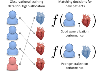
Figure 1: Donor-recipient matching for organ transplantation. We show an exemplary training data set with two types of donors and recipients (red and blue in either case). In current practice, blue recipients are consistently allocated red organs, and vice versa; hence we only observe blue-red and red-blue matches in training data. Using a supervised learning model $f$ to predict transplant outcomes for alternative allocations would provide accurate predictions for blue-red/red-blue matches but would generalize poorly to blue-blue/red-red matches, making it challenging to learn new allocation rules from the training data.

 

While some of the clinical factors pertaining to organ compatibility are already known, e.g., blood and tissue types (Delmonico et al., 2004), it is hypothesized that donor-recipient compatibility involves additional clinical factors and exhibits a much more intricate pattern of feature interaction (Gentry et al., 2011). Uncovering such factors and patterns using organ allocation trials is infeasible and unethical– this motivates a data-driven approach for learning donor-recipient compatibility using (historical) observational data for organ allocations and transplant outcomes.

In this paper, we formulate the learning problem of estimating organ compatibility using observational data for previous donor-recipient matches. This problem departs from the standard supervised learning setup in two ways. First, it involves learning a function that is defined over two feature spaces (for donors and recipients), one of which (the donor feature) can be thought of as an interventional variable. Second, learning the compatibility function requires estimating the transplant outcomes under counterfactual matches not observed in the data (Figure 1). This problem also departs from the treatment effect estimation setup (e.g., (Alaa and van der Schaar, 2017; Alaa and Schaar, 2018; Shalit et al., 2017; Yao et al., 2018; Zhang et al., 2020)) in that the interventional variable (donor features) is potentially continuous-valued and high-dimensional, which render existing solutions based on the binary potential outcomes framework inapplicable.

To address this problem, we propose a model based on representation learning to predict donor-recipient compatibility. The proposed representation addresses the problem of the high-dimensional donor feature space by clustering all donors into a set of donor “types”—it then applies a donor-invariant transformation to the recipient features to predict outcomes for a given instance of a donor-recipient match. The donor-invariant representation is learned by minimizing the probability distance between the feature distribution of all recipients and those of recipients matched with each type of donor. This “domain-adaptation” approach enables the overall predictive model to generalize well when tested on multiple potential matches for new patients, including matches rarely observed in the data. We call this approach: matching representation learning.

We use a deep embedded clustering network (Xie et al., 2016) to learn the donor type clusters and a standard feed-forward network to learn the donor-invariant representations. The features learned by our matching representation are then passed to a multi-headed predictive neural network that predicts the transplant outcome for a given recipient under all possible donor types—the entire model is jointly trained end-to-end. As we show in Section 4, experiments datasets demonstrate that our model outperforms state-of-art allocation methods and policies executed by human experts.

Ethical considerations. The problem of allocation and prioritization of scarce donor organs to terminally-ill patients is associated with ethical issues (Abouna, 2003). The goal of this work is to provide tools for understanding organ compatibility and informing matching decisions rather than fully automating the process.

2 PROBLEM FORMULATION

2.1 Organ transplantation data

Let $\mathcal{X}_{r}$ and $\mathcal{X}_{o}$ be two feature spaces of dimensions $d_{r}$ and $d_{o}$, respectively. Let $x_{r}\in\mathcal{X}_{r}$ and $x_{o}\in\mathcal{X}_{o}$ be two feature instances for a recipient and an organ donor — our key objective is to estimate a compatibility function $C(x_{r},x_{o}):\mathcal{X}_{r}\times\mathcal{X}_{o}\to\mathcal{Y}$ that maps the recipient and donor features to a transplant outcome $y\in\mathcal{Y}$. The transplant outcome $y$ can be defined as the transplant success probability or post-transplant survival time.

Typically, we are presented with an observational data set $\mathcal{D}_{n}$ comprising $n$ pairs of recipients and donors, i.e.,

$$\mathcal{D}_{n}\triangleq\left\{x^{(i)}_{r},x^{(i)}_{o},y^{(i)}\right\}^{n}_{i=1},$$ (1)

and our learning task entails estimating $C(x_{r},x_{o})$ using the samples in $\mathcal{D}_{n}$. Note that each donor-recipient pair $(x^{(i)}_{r},x^{(i)}_{o})$ in $\mathcal{D}_{n}$ is matched according to an underlying process that depends on donor organ availability and existing clinical guidelines on organ matching criteria, e.g., blood and tissue types (Israni et al., 2014). However, donors and recipients in $\mathcal{D}_{n}$ could have been matched differently— an accurate estimate of the compatibility function, $C(x^{(i)}_{r},x^{(j)}_{o}),\forall i\neq j,$ may inform clinicians of an alternative match that would have improved patient outcomes. (For notational brevity, we drop the superscript $i$ in the remainder of the paper.)

2.2 Learning to match with little supervision

The (joint) distribution of donors and recipients in $\mathcal{D}_{n}$ depends on: the distribution of patients $\mathbb{P}(x_{r})$, in addition to the distribution of available donors along with the underlying matching policy, both absorbed into a conditional matching distribution $\mathbb{P}(x_{o}\,|\,x_{r})$, i.e.,

$$\mathbb{P}(x_{o},x_{r})=\mathbb{P}(X_{o}=x_{o}\,|\,X_{r}=x_{r})\cdot\mathbb{P}(X_{r}=x_{r}).$$

Note that the matching distribution $\mathbb{P}(X_{o}=x_{o}\,|\,X_{r}=x_{r})$ is not known ahead of time—it depends on the organs available to recipients at the time of their surgery and the process (clinical guidelines) by which clinicians match donor organs and recipients.

Now consider an estimate $\widehat{C}$ of the compatibility function $C$—the loss function associated with $\widehat{C}$ is:

$$L(\widehat{C})=\mathbb{E}_{X_{r}}\mathbb{E}_{X_{o}}\ell(y,\widehat{C}(X_{r},X_{o})),$$ (2)

where $\ell(.)$ is the loss associated with a donor-recipient feature instance, and $L$ is the expected loss for $\widehat{C}$.

We note that the loss function in (2) is independent of the matching distribution $\mathbb{P}(x_{o}\,|\,x_{r})$. That is, we average the instance-wise loss $\ell(y,\widehat{C})$ over the marginal distributions of donors and recipients, $\mathbb{P}(x_{o})$ and $\mathbb{P}(x_{r})$, rather than their joint distribution $\mathbb{P}(x_{o},x_{r})$. This is because our estimate $\widehat{C}$ is meant to be used to predict transplant outcomes under alternative matches different from the ones observed in the data. In other words, we want our estimate $\widehat{C}$ to generalize well for all possible pairs of donors and recipients, not just the pairs that are frequently matched in the observational data.

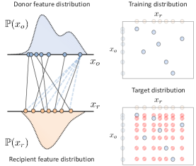
Figure 2: Illustration for the donor-recipient matching problem. Here, solid black lines correspond to factual matches and dotted blue ones correspond to counterfactual matches (left). The right panel shows the empirical training/target distributions—blue dots correspond to observed transplant outcomes whereas red dots are transplant outcomes for all of the (unobserved) counterfactual matches.

 

Why is learning the compatibility function $C(x_{r},x_{o})$ not a standard supervised learning problem? The reason we cannot simply use supervised methods to learn $C$ is because of the discrepancy between the distribution of donor-recipient pairs in the training data, and the target distribution of donor organs and recipients to which the model will be practically applied, i.e.,

Training distribution: $$\,\,\,\mathbb{P}(X_{r},X_{o}),$$

Target distribution: $$\,\,\,\mathbb{P}(X_{r})\cdot\mathbb{P}(X_{o}).$$

That is, we want to train the model on data samples of (already-matched) donor-recipient pairs, but then apply the model to predict outcomes of all possible donor-recipient matches in order to inform matching decisions (See Figure 2). If we are to use supervised learning via empirical loss minimization, the empirical risk $\widehat{L}$ for an estimate $\widehat{C}$ would be

$$\widehat{L}(\widehat{C})=\sum_{i}\ell(y^{(i)},\widehat{C}^{(i)})+\sum_{i\neq j}\underbrace{\ell(y^{(i,j)},\widehat{C}(x^{(i)}_{r},x^{(j)}_{o}))}_{\mbox{Counterfactual match}},$$

where $y^{(i,j)}$ is the true transplant outcome for recipient $i$ having been given donor $j$’s organ. Thus, evaluating the empirical loss $\widehat{L}(\widehat{C})$ entails evaluating the instance-wise loss of all the $n^{2}$ possible matches between donors and recipients. However, we only observe $n$ “factual” matches in $\mathcal{D}_{n}$; the remaining $n^{2}-n$ donor-recipient matches are “counterfactual”, and so we do not observe any transplant outcome $y^{(i,j)}$ except for $i=j$, rendering empirical risk minimization infeasible.

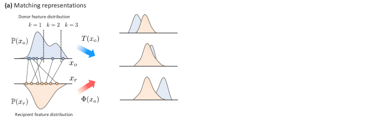
Figure 3: Pictorial depiction of matching representation. (a) Here, we show the same distributions for donor and recipient features as in Figure 2. (We show one-dimensional feature spaces $\mathcal{X}_{r}$ and $\mathcal{X}_{o}$ for simplicity of exposition.) The donor type map $T(.)$ clusters the donor feature space into 3 distinct clusters. Because the matching distribution $\mathbb{P}(X_{o}|X_{r})$ is not equal to $\mathbb{P}(X_{o})$, the conditional distribution of recipient features given the matched donor types are different. (For example, the age distribution for patients receiving kidneys from donors with blood type A is different from that of patients matched to donors with blood type B.) The mapping $\Phi$ transforms $X_{r}$ to a random variable $X^{\prime}$ with a distribution that is invariant to the donor type. (b) Architecture for our model. The recipient feature is passed through the mapping $\Phi$ and the donor feature is passed through $T$, both implemented through a feed-forward neural network. The output of $\Phi$, $x^{\prime}$, is passed through a multi-headed neural network, with each head predicting the transplant outcome under different donor types.

 

3 MATCHING REPRESENTATIONS

As we have seen in Section 2, learning the compatibility function $C(x_{r},x_{o})$ via empirical risk minimization is not possible as the empirical estimate of (2) is inaccessible. To address this challenge, we develop a model for estimating $C$ using matching representations that neutralize the bias induced by the matching distribution $\mathbb{P}(x_{o}\,|\,x_{r})$, and generalizes well to the marginal distributions of all donors and recipients.

3.1 Match-Invariant Representations

The discrepancy between the training (or source) and target distributions renders our learning problem akin to domain adaptation; a key technique in this setup is the usage of domain-invariant representations to alleviate the generalization errors resulting from distribution mismatches (Shalit et al., 2017; Zhao et al., 2019).

Building on the concept of domain-invariance, we define a match-invariant representation ${\bf\Phi}:\mathcal{X}_{r}\times\mathcal{X}_{o}\to\mathcal{Z}$ as one that satisfies the following condition:

$$\mathbb{E}_{\mathbb{P}(X_{r},X_{o})}\,f({\bf\Phi}(X_{r},X_{o}))=\mathbb{E}_{\mathbb{P}(X_{r})\,\mathbb{P}(X_{o})}f({\bf\Phi}(X_{r},X_{o})),$$

for some function $f$. That is, the representation ${\bf\Phi}$ alleviates the (confounding) effect of the matching distribution $\mathbb{P}(x_{o}\,|\,x_{r})$, enabling models trained on transformed donor-recipient features, ${\bf\Phi}(X_{r},X_{o})$, to generalize to the target distribution. The match-invariance condition plays a key role in the matching representations that we construct throughout this Section.

3.2 Latent Donor Types

Constructing a match-invariant representation ${\bf\Phi}$ is a complicated task, especially when the donor and recipient feature spaces, $\mathcal{X}_{r}$ and $\mathcal{X}_{o}$, are high-dimensional. To simplify the design of ${\bf\Phi}$, we assume that donors belong to a set of $K$ “types”. Let $T:\mathcal{X}_{o}\to\{1,\ldots,K\}$ be a map from donor features to discrete donor types; the matching distribution with respect to donor types can be given by $\mathbb{P}(T(x_{o})=k\,\,|\,x_{r}),\,k\in\{1,\ldots,K\}$.

The donor type map $T$ is not predefined ahead of time, but is rather learned from the data as part of the representation ${\bf\Phi}$. The clustering of donors is not only useful for simplifying the construction of matching representations, but also for providing interpretable grouping of donor types that could be conveniently incorporated in clinical guidelines (Barr et al., 2006).

3.3 Building Matching Representations

We propose the following construction for a matching representation ${\bf\Phi}:\mathcal{X}_{r}\times\mathcal{X}_{o}\to\mathcal{Z}$ that satisfies the invariance condition in Section 3.1. The proposed representation converts the feature pair $(x_{r},x_{o})\in\mathcal{X}_{r}\times\mathcal{X}_{o}$ to $z=(x^{\prime},k)\in\mathcal{Z}$ through the transformation

$${\bf\Phi}(x_{r},x_{o})=(x^{\prime},k)=(\Phi(x_{r}),\,T(x_{o})).$$ (3)

The mapping in (3) jointly transforms the donor feature $x_{o}$ to donor type $k$, and recipient feature $x_{r}\in\mathcal{X}_{r}$ to $x^{\prime}\in\mathcal{X}^{\prime}$. The mapping $\Phi:\mathcal{X}_{r}\to\mathcal{X}^{\prime}$ is designed to ensure that ${\bf\Phi}$ satisfies match-invariance, which in the case of a clustered donor feature space reduces to:

$$\mathbb{E}_{X_{r}}\,f(\Phi(X_{r}))=\mathbb{E}_{X_{r}|T(X_{o})=k}\,f(\Phi(X_{r})),$$ (4)

for all $X_{o}\in\mathcal{X}_{o},\,T(X_{o})=k,\,\forall k\in\{1,\ldots,K\}$. That is, the mapping $\Phi$ transforms $X_{r}$ to a new feature space wherein the distributions of $\Phi(X_{r})\,|\,T(X_{o})=k$ are the same for all latent donor types $k\in\{1,\ldots,K\}$.

Figure 3(a) pictorially visualizes the matching representation ${\bf\Phi}$ in the donor-recipient feature space. As we can see, ${\bf\Phi}$ discretizes the donor feature space $\mathcal{X}_{o}$ into three distinct clusters (donor types). The distribution of recipients $X_{r}$ matched to organs from each donor cluster differ significantly—the mapping $X^{\prime}=\Phi(X_{r})$ transforms $X_{r}$ to a new feature space where the distributions $X^{\prime}\,|\,T(X_{o})=k,\forall k\in\{1,2,3\}$ are similar.

3.4 Learning compatibility functions with matching representations

Having constructed a matching representation for the donor-recipient features, we estimate the compatibility function $C(x_{r},x_{o})$ in the transformed feature space $\mathcal{Z}$ rather than $\mathcal{X}_{r}\times\mathcal{X}_{o}$ as follows:

$$\widehat{C}(x_{r},x_{o})=f({\bf\Phi}(x_{r},x_{o}))=f(x^{\prime},k),$$ (5)

where $f:\mathcal{Z}\to\mathcal{Y}$ is a predictive model that maps the transformed (donor-recipient) features $z$ to transplant outcome $y$. Thus, our model comprises two learnable components: the predictive model $f$, and the matching representation ${\bf\Phi}$. In what follows, we provide the model specification for $f$ and ${\bf\Phi}$.

Multi-headed predictive network. Given a matching representation, we model $f({\bf\Phi}(x_{r},x_{o}))=f(x^{\prime},k)$ as a multi-headed neural network model, where we use $K$ feed-forward neural networks to predict the transplant outcome under each type of donor for a given recipient with a feature $x_{r}$ (See Figure 3(b)). We denote the predictive loss associated with $f$ as $L_{f}$.

Donor type mapping via deep embedded clustering. Clustering the donor space is an unsupervised problem as the donor types are not defined or labeled. We use a Deep Embedded Clustering (DEC) network (Xie et al., 2016) to model the donor type mapping $T(x_{o})$. Our choice of DEC is motivated by the ease of its incorporation into an end-to-end training procedure that involves the other model components ($\Phi$ and $f$).

DEC involves training an autoencoder at first to learn a representation of donor features. The encoder part of the autoencoder is then used to learn a clustering using the following loss function:

$$t_{ij} =\frac{(1+||{\bf d}_{i}-\mathbf{\mu}_{j}||^{2})^{-\frac{1}{2}}}{\sum_{j}(1+||\mathbf{d}_{i}-\mathbf{\mu}_{j}||^{2})^{-\frac{1}{2}}},\,\,p_{ij}=\frac{\frac{t_{ij}^{2}}{\sum_{i}t_{ij}}}{\sum_{j}\frac{t_{ij}^{2}}{\sum_{i}t_{ij}}}$$

$$L_{DEC} =\sum_{i}\sum_{j}p_{ij}\log\frac{p_{ij}}{t_{ij}}$$ (6)

where $\mathbf{d}_{i}$ is the learned representation of donor $i$ (produced by the encoder), $\mathbf{\mu}_{j}$ is a cluster center (which is randomly initialized), and $t_{ij}$ represent the probability of donor $i$ belonging to cluster $j$.

Matching representations using probability distance minimization. Finally, the last component of our model is the feature map $\Phi:\mathcal{X}_{r}\to\mathcal{X}^{\prime}$, which we model via a (feed-forward) neural network. To achieve the match-invariance condition in (4), we learn $\Phi$ by minimizing the distance among distributions of representations of recipients assigned to different types of donors through the following loss function:

$$L_{\Phi}=\sum^{K}_{k=1}d(\mathbb{P}_{X_{r}}(\Phi),\mathbb{P}_{X_{r}|T(X_{o})=k}(\Phi)),$$ (7)

where $\mathbb{P}(\Phi)=\mathbb{P}(\Phi(X_{r}))$ ($X_{r}$ is dropped for notational brevity), and $d(.,.)$ is a probability distance metric, such as the integral probability metrics (IPM) (Müller, 1997), total variation distance or KL divergence. Here, we use the KL divergence metric assuming that the distributions of $X_{r}$ and $X_{r}\,|\,T(X_{o})$ are Gaussian.

The overall model is trained end-to-end by combining the loss functions $L_{f}$, $L_{DEC}$, and $L_{\Phi}$, as follows:

$$L=\sum L_{f}+\alpha\cdot L_{DEC}+\beta\cdot L_{\Phi}$$ (8)

where $\alpha$ and $\beta$ are hyperparameters balancing losses of different components of the model. We also treat the number of donor types $K$ as a hyperparameter.

4 RELATED WORKS

Our work relates to two strands of previous literature: (1) machine learning-based models for transplantation, and (2) models for estimating treatment effects. In this Section, we explain how our work relates to these.

Machine learning-based models for organ transplantation. Previous works on organ transplants focus on developing a more accurate risk model for predicting survival after transplant (Medved et al., 2018; Nilsson et al., 2015). In (Nilsson et al., 2015), a deep neural network is proposed with classification and regression trees to predict transplantation outcomes and evaluate the impact of recipient-donor variables on survival. Instead of improving the accuracy of prediction of survival, other works focus on improving recipient-donor matching. For instance, (Yoon et al., 2017) partition recipient-donor feature space into subspaces and use a separate prediction model for each subspace. In this architecture, each independent prediction model is trained to solve a more specific and less general sub-problem. Therefore, models for subspaces of matched recipient-donor pairs are expected to be more robust than models trained to solve the general problem. Unlike our model, this approach does not handle the matching bias in the data, hence it cannot be reliably used to recommend alternative matches other than those observed in the data.

Estimating treatment effects. The problem of estimating the effects of treatments from observational data shares similarities with our setup—in this setup, the effects of a treatment are estimated by inferring its counterfactual outcomes while accounting for the selection bias resulting from the data being generated according to an underlying treatment policy. A typical approach in existing literature is to fit a single model to estimate all counterfactuals outcomes of a treatment, and distributions of different treatments’ populations are adjusted (balanced) to handle selection bias. For instance, (Wager and Athey, 2018) uses random forest, and (Johansson et al., 2016; Shalit et al., 2017) use deep neural networks to solve treatment effects estimation problem under this single model methodology. On the contrary, (Alaa and van der Schaar, 2017; Alaa et al., 2017) use multi-task approaches that are analogous to our multi-headed predictive network, such as multi-task Gaussian process, to estimate treatment effects. Our proposed model is most similar to (Alaa et al., 2017) and (Shalit et al., 2017), since in all these works, deep neural networks with multiple heads are used to estimate potential outcomes. However, these works focus on binary treatment effects, hence they cannot handle the continuous, high-dimensional interventions in our setting (donor features).

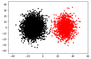
(a) Distribution of recipients.

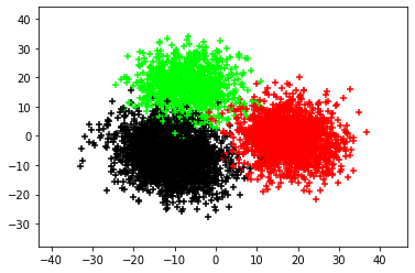
(b) Distribution of donors.

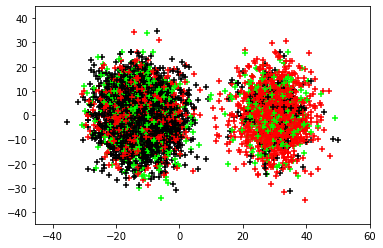
(c) Donor-recipient pairs.

Figure 4: Distributions of recipient and donor features for the synthetic model in Section 5.1. In (a), Black denotes $m=1$ and Red denotes $m=2$. In (b) and (c), Black denotes $k=1$, Red denotes $k=2$, and Green denotes $k=3$.

 

5 EXPERIMENTS

Since we never observe all counterfactual matches in the real world, there is no ground truth target (label) to evaluate estimated donor-recipient compatibility in matches other than the ones observed in data. Hence, it is difficult to evaluate the performances of models using only real-world data. Previous works on related problems involving counterfactual inference use semi-synthetic data comprising real covariates and simulated outcomes to evaluate performance (e.g., (Pearl, 2009; Louizos et al., 2017; Shalit et al., 2017; Yoon et al., 2018)). In this Section, we use synthetic and semi-synthetic data sets to quantitatively evaluate the performance of our proposed model. We also use real-world data sets to qualitatively test the performance of our model under real circumstances.

5.1 Experiments on synthetic data

We evaluate the proposed matching representation on a synthetic data set to demonstrate its ability to discover the “optimal” clustering of donor types and better allocation policies from observational data.

We generate the synthetic data from a Gaussian mixture model, with a mixture of 2 recipient types and 3 donor types—we denote the recipient type as $m$ and the donor type as $k$. Recipients of different types have different probabilities of pairing with donors of different types as follows:

$\mathbb{P}(k\mid m)$	$k=1$	$k=2$	$k=3$
$m=1$	0.6	0.2	0.2
$m=2$	0.1	0.7	0.2

The data set contains selection bias since pairing of recipients from $m=2$ and donors from $k=1$ is rarely observed, hence the conditional distributions of recipients assigned to donor types are unbalanced.

The transplantation outcome $y$ (survival time) associated with each donor-recipient match is modeled as:

$$y\mid m=1 \sim\mathcal{N}\left(\begin{bmatrix}500\\ 1000\\ 1100\end{bmatrix},\begin{bmatrix}50&0&0\\ 0&100&0&\\ 0&0&100\end{bmatrix}\right),$$

$$y\mid m=2 \sim\mathcal{N}\left(\begin{bmatrix}100\\ 800\\ 900\end{bmatrix},\begin{bmatrix}10&0&0\\ 0&100&0&\\ 0&0&100\end{bmatrix}\right).$$

The synthetic data is designed so that donor types 2 and 3 are “similar” and lead to similar transplantation outcomes for all recipients. Besides, recipients of type 1 are more likely to be paired with donors of type 1, despite the fact that donors of types 2 and 3 are better matches for the recipients. We sample 5,000 recipient-donor pairs and run several simulations on the synthetic data set to compare the allocation policy of our model and other state-of-art allocation policies.

Table 1: Simulation results of allocation policies evaluated on the synthetic data set. flipped ratio stands for the ratio of Type-1 recipients that are paired with Type-1 donors but now assigned to other type of donors. High flipped ratio indicates that the policy can discover the better potential policy from the data set.

Policy	All Recipients			Type-1 Recipients
	death rate	avg survival	avg benefit	flipped ratio	avg survival
FCFS	0.34	470.57	104.74	n.a.	n.a.
UF	0.34	470.47	104.55	n.a.	n.a.
BF	0.27	514.95	177.04	n.a.	n.a.
Real	0.34	474.28	104.10	0.00	508.97
Matching rep. (FCFS)	0.30	501.56	133.30	0.46	732.41
Matching rep. (UF)	0.30	514.98	131.98	0.53	769.43
Matching rep. (BF)	0.28	528.43	165.57	0.41	710.50

We consider the following organ allocation policies:

(a) Real policy: a new donor organ is allocated based on expert knowledge. This is the underlying policy by which the observational data was generated.

(b) First come first serve (FCFS): a new donor is always allocated to the first recipient in the waiting list.

(c) Utility first: a new donor organ is allocated to the recipient with the best predicted transplantation outcome (survival time after transplantation).

(d) Benefit first: a new donor organ is allocated to the recipient with highest benefit, where benefit is defined as the predicted gain in survival time after transplant.

We simulate these policies by examining the sampled donors and recipients in sequence and applying the allocation rules above. The performances of policies are evaluated in terms of recipients’ average survival time after surgery, recipients’ average net benefit in survival time of conducting surgery, and the death rate of recipients waiting in the sequence. A robust allocation policy is expected to have high average survival time and low death rate. Results are reported in Table 1. We also visualize the clusters learned by our matching representations model in Figure 5(b).

As shown in Figure 5(b), the clustering inferred by our matching representations merges the 2 “similar” donor types into a single cluster, which improves the interpretability of the underlying data. Additionally, as shown in Table 1, our model outperforms the baseline allocation policies in terms of the achieved survival time/rate. Matching representations achieve the highest average survival time as well as comparable death rate, compared with the best benchmark. In comparison with the real allocation policy of the dataset, it extended the average survival time by 11.4%, the average benefit by 59%, and reduced death rate by 6%.

(a) Original clusters

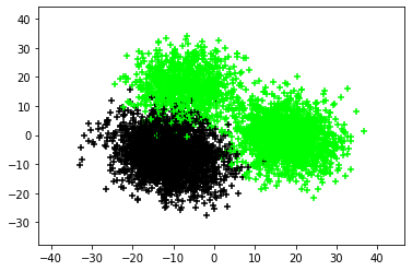
(b) Trained clusters

Figure 5: Visualization for the learned donor type clusters compared to the original clusters in the sampled data set. Black denotes $k=1$, Red denotes $k=2$, and Green denotes $k=3$. Donor types $Ok=2$ and $k=3$ are merged together in the jointly trained clustering model.

 

It is also noticable that about 50% of Type-1 recipients originally assigned to Type-1 donors are assigned to donors of different types by our model. For this group of recipients, the flipping of assignments leads to a significant improvement of survival time for 51.2%. The results suggest that our model is capable of discovering the better potential allocation policy from the observed data set, by clustering donors and constraining recipients to match the best type of donors.

Table 2: Simulation results of allocation policies. Simulations are run on PLTSD and UNOS datasets.

Policy	PLTSD			UNOS-HR			UNOS-LU
	Death rate	Avg. benefit	Avg. survival	Death rate	Avg. benefit	Avg. survival	Death rate	Avg. benefit	Avg. survival
FCFS	0.25	700.75	1271.54	0.18	324.01	1959.47	0.18	213.52	1156.85
UF	0.24	721.70	1295.21	0.21	203.35	2065.85	0.23	108.58	1210.71
BF	0.23	737.24	1306.01	0.16	377.71	2113.22	0.15	273.15	1288.77
Real	0.25	703.23	1280.41	0.18	325.52	1974.74	0.18	219.46	1177.54
Matching rep. (FCFS)	0.24	720.69	1285.09	0.16	357.20	2011.88	0.16	260.29	1193.32
Matching rep. (UF)	0.24	730.85	1299.74	0.16	320.53	2057.54	0.19	177.14	1216.79
Matching rep. (BF)	0.23	736.98	1305.16	0.16	389.69	2024.33	0.15	225.61	1224.48

5.2 Liver, lung and heart transplant data

Next, we test our model using three real-world datasets for organ transplantation. The first is the Paired Liver Transplant Standard Dataset (PLTSD), a database in which donor-recipient pairs are extracted from the NHS Liver Transplant Standard Dataset. This dataset contains 6,898 pairs of donors and recipients—recipients are characterized by 55 features, whereas donors have 28 features. The second dataset is the lung transplant data set from UNOS, which comprises two sub-datasets: a set of 60,400 recipients who underwent heart transplantation, and 29,210 recipients who underwent lung transplantation over the years from 1987 to 2015, with 37 donor-recipient features in each.

Because these are real-world data sets, we only observe transplant outcomes for factual donor-recipient matching but not for the counterfactual ones. Therefore, we simulate the transplant outcomes under counterfactual matches via a semi-synthetic model (See Appendix). We run experiments to evaluate the precision of estimated factual transplant outcomes, in addition to the precision of estimated potential outcomes under counterfactual matches. We use several evaluation metrics: (1) precision of estimated factual outcomes $\epsilon_{F}$; (2) precision of estimated potential outcomes $\epsilon_{WMSE}$; (3) accuracy of the best donor type $AoDT$.

$$\epsilon_{F} =\frac{1}{n}\sum_{i=1}^{n}({\bf\hat{y}}^{(i)}[k^{(i)}]-y^{(i)})^{2},$$

$$\epsilon_{WMSE} =\frac{1}{n}\sum_{i=1}^{n}\boldsymbol{1}^{\intercal}_{1\times K}\,({\bf\hat{y}}^{(i)}-{\bf y}^{(i)})^{2},$$

$$AoDT =\frac{1}{n}\sum_{i=1}^{n}\max_{k}\hat{\mathbf{y}}^{(j)}[k],$$

where ${\bf\hat{y}}^{(i)}[k^{(i)}]=\widehat{C}(x_{r}^{(i)},T(x_{o}^{(i)})=k^{(i)})$ and ${\bf y}^{(i)}$ is a $1\times K$ vector of outcomes under each donor type.

To our knowledge, there is no existing baselines that has an equivalent problem formulation to ours. Therefore, we use baselines sharing the same fundamental structure of our proposed model, where there is a clustering component to classify donors as well as a counterfactual estimation component to estimate potential outcomes. We use K-Means, EM, and DEC clusters as baselines for the clustering component. Baseline clusters are independent of the counterfactual estimation task, and they are not jointly trained with the counterfactual estimation component. For the predictive component, we utilize a linear regression and a multi-headed neural net as baselines. We also compare allocation policies (similar to those considered in Section 5.1) based on our model to baselines based on several state-of-art regression models, namely Regression Neural Network (RegNN) (Specht, 1991), Regression Tree (RegTree) (Strobl et al., 2009), LASSO Regression Tibshirani (1996), Ridge Regression (Hoerl and Kennard, 1970), and ElasticNet Regression (Zou and Hastie, 2005). Results are reported in Table 3. Data is divided into 90%/10% training/validating sets. Results are given in Tables 2, 3 and 4.

Table 3: Simulation results of allocation policies. Simulations are run on PLTSD dataset.

Policy	avg survival	avg benefit	death rate
Real	1280.4136	703.234	0.2489
FCFS	1271.5453	700.754	0.2493
UF	1295.2122	721.700	0.2419
BF	1306.0093	737.245	0.2360
RegNN	1271.1415	700.516	0.2495
RegTree	1276.1471	704.6127	0.2481
LASSO	1293.5784	719.112	0.2445
Ridge	1297.4642	723.233	0.2425
ElasticNet	1283.6174	707.714	0.2470
Matching rep. (FCFS)	1285.0895	720.687	0.2431
Matching rep. (UF)	1299.7383	730.849	0.2396
Matching rep. (BF)	1305.1631	736.984	0.2366

Table 4: Performance of all baselines on PLTSD. The results reported are averaged over 50 trials.

Model	$\epsilon_{F}$	$\epsilon_{WMSE}$	$AoDT$
K-Means/Linear	15.5229	14.7163
EM/Linear	15.5218	14.7108
DEC/Linear	15.5227	14.7680
K-Means/NN	14.6295	13.8614	.5962
with rep.	14.6399	13.9016	.5735
EM/NN	14.5779	13.9918	.5504
with rep.	14.6302	13.9623	.5567
DEC/NN	14.5840	13.7966	.5965
with rep.	14.5711	13.8430	.6017
Matching rep.	14.5362	14.0140	.6260

As shown in Tables 2 and 3, our model shows comparable results to the best allocation policy BF, which significantly outperforms all other policies. Compared with the real policy, we observe that 5,224 out of the 6,898 (75.7%) donors are assigned a different recipient by our model—in addition, our model extends the average survival time by 25 days (2%) and the average benefit for 34 days (4.8%). Our model also reduces the death rate by 4.9%.

As shown in Table 4, our model outperforms benchmark models in many aspects. It is observable that our model produce better precisions with and without representation loss. For our proposed model, precision of estimated factual outcome improved by 3.4% in PLTSD and FPLTSD respectively, compared to the best benchmark. As for $AoDT$, our model achieves the highest AoDT of 62.60%, which improved by 4% from the best benchmark and improved by 87.82% compared to random guessing of donor-recipient matches.

6 Conclusion

In this paper, we developed a novel method for learning the compatibility between donors and recipients in the context of organ transplantation. The key challenge in this problem is that the underlying matching policies, driven by clinical guidelines, creates a “matching bias”, and hence a co-variate shift in the joint distribution of donor and recipient features. To solve this problem, we developed a learning approach based on matching representations to learn a donor-recipient compatibility function that generalizes well to the marginal distributions of donors and recipients. Our approach learns feature representations by jointly clustering donor features, and applying donor-invariant transformations to recipient features to predict outcomes for a given donor-recipient instance. Experiments on multiple datasets show that our model outperforms state-of-art organ allocation methods.

Acknowledgments

We would like to thank the reviewers for their invaluable feedback and the NHS Blood and Transplant for providing data. This work was supported by The Alan Turing Institute (ATI) under the EPSRC grant EP/N510129/1, The US Office of Naval Research (ONR), and the National Science Foundation (NSF).

References

- Abouna (2003) George M Abouna. Ethical issues in organ transplantation. Medical Principles and Practice, 12(1):54–69, 2003.
- Alaa and Schaar (2018) Ahmed Alaa and Mihaela Schaar. Limits of estimating heterogeneous treatment effects: Guidelines for practical algorithm design. In International Conference on Machine Learning, pages 129–138, 2018.
- Alaa and van der Schaar (2017) Ahmed M. Alaa and Mihaela van der Schaar. Bayesian inference of individualized treatment effects using multi-task gaussian processes. In Advances in Neural Information Processing Systems 30, pages 3424–3432. 2017.
- Alaa et al. (2017) Ahmed M. Alaa, Michael Weisz, and Mihaela van der Schaar. Deep counterfactual networks with propensity-dropout. 2017.
- Barr et al. (2006) Mark L Barr, Jacques Belghiti, Federico G Villamil, Elizabeth A Pomfret, David S Sutherland, Rainer W Gruessner, Alan N Langnas, and Francis L Delmonico. A report of the vancouver forum on the care of the live organ donor: lung, liver, pancreas, and intestine data and medical guidelines. Transplantation, 81(10):1373–1385, 2006.
- Briceño et al. (2013) Javier Briceño, Ruben Ciria, and Manuel de la Mata. Donor-recipient matching: myths and realities. Journal of hepatology, 58(4):811–820, 2013.
- Delmonico et al. (2004) Francis L Delmonico, Paul E Morrissey, George S Lipkowitz, Jeffrey S Stoff, Jonathan Himmelfarb, William Harmon, Martha Pavlakis, Helen Mah, Jane Goguen, Richard Luskin, et al. Donor kidney exchanges. American Journal of Transplantation, 4(10):1628–1634, 2004.
- Gentry et al. (2011) Sommer E Gentry, Robert A Montgomery, and Dorry L Segev. Kidney paired donation: fundamentals, limitations, and expansions. American journal of kidney diseases, 57(1):144–151, 2011.
- Hoerl and Kennard (1970) Arthur E. Hoerl and Robert W. Kennard. Ridge regression: Biased estimation for nonorthogonal problems. 12(1):55–67, 1970.
- Israni et al. (2014) Ajay K Israni, Nicholas Salkowski, Sally Gustafson, Jon J Snyder, John J Friedewald, Richard N Formica, Xinyue Wang, Eugene Shteyn, Wida Cherikh, Darren Stewart, et al. New national allocation policy for deceased donor kidneys in the united states and possible effect on patient outcomes. Journal of the American Society of Nephrology, 25(8):1842–1848, 2014.
- Johansson et al. (2016) Fredrik Johansson, Uri Shalit, and David Sontag. Learning representations for counterfactual inference. In International conference on machine learning, pages 3020–3029, 2016.
- Lechler et al. (2005) Robert I Lechler, Megan Sykes, Angus W Thomson, and Laurence A Turka. Organ transplantation—how much of the promise has been realized? Nature medicine, 11(6):605–613, 2005.
- Louizos et al. (2017) Christos Louizos, Uri Shalit, Joris M. Mooij, David Sontag, Richard Zemel, and Max Welling. Causal effect inference with deep latent-variable models. In Advances in Neural Information Processing Systems, pages 6446–6456, 2017.
- Medved et al. (2018) Dennis Medved, Mattias Ohlsson, Peter Höglund, Bodil Andersson, Pierre Nugues, and Johan Nilsson. Improving prediction of heart transplantation outcome using deep learning techniques. 8(1):3613, 2018.
- Müller (1997) Alfred Müller. Integral probability metrics and their generating classes of functions. In Advances in Applied Probability, pages 429–443, 1997.
- Nilsson et al. (2015) Johan Nilsson, Mattias Ohlsson, Peter Höglund, Björn Ekmehag, Bansi Koul, and Bodil Andersson. The international heart transplant survival algorithm (IHTSA): A new model to improve organ sharing and survival. 10(3):e0118644, 2015.
- Pearl (2009) Judea Pearl. Causality. Cambridge university press, 2009.
- Rubin (2002) Robert H Rubin. Infection in the organ transplant recipient. In Clinical approach to infection in the compromised host, pages 573–679. Springer, 2002.
- Shalit et al. (2017) Uri Shalit, Fredrik D. Johansson, and David Sontag. Estimating individual treatment effect: generalization bounds and algorithms. In International Conference on Machine Learning, pages 3076–3085, 2017.
- Specht (1991) Donald F. Specht. A general regression neural network. 2(6):568–576, 1991.
- Strobl et al. (2009) Carolin Strobl, James Malley, and Gerhard Tutz. An introduction to recursive partitioning: Rationale, application, and characteristics of classification and regression trees, bagging, and random forests. 14(4):323–348, 2009.
- Tibshirani (1996) Robert Tibshirani. Regression shrinkage and selection via the lasso. 58(1):267–288, 1996.
- Wager and Athey (2018) Stefan Wager and Susan Athey. Estimation and inference of heterogeneous treatment effects using random forests. 113(523):1228–1242, 2018.
- Xie et al. (2016) Junyuan Xie, Ross Girshick, and Ali Farhadi. Unsupervised deep embedding for clustering analysis. In International conference on machine learning, pages 478–487, 2016.
- Yao et al. (2018) Liuyi Yao, Sheng Li, Yaliang Li, Mengdi Huai, Jing Gao, and Aidong Zhang. Representation learning for treatment effect estimation from observational data. In Advances in Neural Information Processing Systems 31, pages 2633–2643. 2018.
- Yoon et al. (2017) Jinsung Yoon, Ahmed M. Alaa, Martin Cadeiras, and Mihaela van der Schaar. Personalized donor-recipient matching for organ transplantation. In Thirty-First AAAI Conference on Artificial Intelligence, 2017.
- Yoon et al. (2018) Jinsung Yoon, James Jordon, and Mihaela van der Schaar. GANITE: Estimation of individualized treatment effects using generative adversarial nets. 2018.
- Zhang et al. (2020) Yao Zhang, Alexis Bellot, and Mihaela van der Schaar. Learning overlapping representations for the estimation of individualized treatment effects. 2020.
- Zhao et al. (2019) Han Zhao, Remi Tachet Des Combes, Kun Zhang, and Geoffrey Gordon. On learning invariant representations for domain adaptation. In International Conference on Machine Learning, pages 7523–7532, 2019.
- Zou and Hastie (2005) Hui Zou and Trevor Hastie. Regularization and variable selection via the elastic net. 67(2):301–320, 2005.