Long-ranged velocity correlations in dense systems of self-propelled particles

Abstract

Model systems of self-propelled particles reproduce many phenomena observed in laboratory active matter systems that defy our thermal equilibrium-based intuition. In particular, in stationary states of self-propelled systems, it is recognized that velocities of different particles exhibit non-trivial equal-time correlations. Such correlations are absent in equivalent equilibrium systems. Recently, researchers found that the range of the velocity correlations increases with increasing persistence time of the self-propulsion and can extend over many particle diameters. Here we review the initial studies of long-ranged velocity correlations in solid-like systems of self-propelled particles. Then, we demonstrate that the long-ranged velocity correlations are also present in dense fluid-like systems. We show that the range of velocity correlations in dense systems of self-propelled particles is determined by the combination of the self-propulsion and the virial bulk modulus that originates from repulsive interparticle interactions.

1 Introduction

A quickly growing field is the study of active matter systems [1, 3, 2, 5, 4, 6, 7]. Individual components of these systems perform persistent motion due to the injection (consumption) of energy from their environment. Examples include cell assemblies [8, 9, 10, 11, 12, 13], bird flocks [2], bacterial suspensions [14, 15, 16, 17, 18, 19, 20], and self-propelled colloids [21, 22, 23, 24, 25, 26, 27, 28]. Active matter systems exhibit many properties absent in equilibrium thermal systems, e.g. they may undergo a phase separation of liquid-gas type in the absence of any attractive interactions [29].

One interesting property, first demonstrated experimentally by Garcia et al. [11], is the presence of equal-time velocity correlations. These correlations are absent in classical equilibrium systems. It has been recognized for some time [30, 32, 31] that such non-trivial equal-time velocity correlations are present in simple microscopic models of active matter systems, i.e. in systems of self-propelled particles. These correlations are an emergent property of these systems, i.e. they appear spontaneously, without any explicit velocity-aligning interactions. Recently, two groups [13, 33] independently found that velocity correlations in dense systems of self-propelled particles can be long-ranged. The analysis and rationalization of these correlations relied upon the solid-like nature of the systems studied. Here we review these studies and present computer simulation results that demonstrate the presence of long-ranged velocity correlations also in dense fluid-like systems. We develop a simple theory that explains the appearance of these correlations through the combined effect of the self-propulsion and the virial bulk modulus of the active fluid. We finish with a brief discussion, emphasizing the features of velocity correlations that the simple theory cannot describe.

2 Long-ranged velocity correlations in dense, ordered systems of self-propelled particles

Caprini et al. [33, 34] investigated $2d$ systems of repulsive, monodisperse, overdamped active Brownian particles (ABPs) [35, 36]. They showed that the previously studied motility-induced phase separation [29] is accompanied by a spontaneous alignment of the velocities of the particles in the dense phase. They found that the dense phase is either hexatic or solid, and that the transition between these two phases influences the alignment. The average size of the domains with aligned velocities was found to grow with increasing persistence time of the self-propulsion. Although the spontaneous alignment of the velocities was mainly discussed in the context of phase separation, Caprini et al. showed that it also occurred in single-phase systems if the density was high enough. While sufficiently high density was important for the appearance of the spontaneous velocity ordering, the size of the ordered domains was growing primarily due to increasing persistence time.

To quantify the observed velocity ordering Caprini et al. introduced and evaluated two correlation functions. Here we focus on velocity correlation function $C(r)$ [34],

$$C(r)=\frac{\left<\mathbf{v}(\mathbf{r})\cdot\mathbf{v}(0)\right>}{\left<v^{2}\right>},$$ (1)

where $\mathbf{v}(\mathbf{r})$ represents the velocity of the particle located at $\mathbf{r}$ (continuous limit is implied). Caprini et al. found that in dense systems $C(r)$ exhibits exponential dependence on $r$. We note that exponentially decaying velocity correlations were found in the experimental study of Garcia et al. [11]. Using $C(r)$, Caprini et al. defined and evaluated the velocity correlation length. They found that it increases as the square root of the persistence time of the self-propulsion, but it is also influenced by the transition between the solid and hexatic phases.

To explain their findings Caprini et al. developed a theory for velocity correlation function $C(r)$ based on the assumption that the dense phase is a $2d$ hexagonally ordered crystal, with particles oscillating around their average positions. While this assumption is appropriate for dense ordered systems investigated in Refs. [33, 34], it is not applicable for fluid-like disordered systems. Caprini et al. showed that their assumption results in the following formula for the large-$r$ behavior of the correlation function,

$$C(r)\propto\frac{\bar{x}^{2}}{\ell^{2}}\left(\frac{\ell}{8\pi r}\right)^{1/2}e^{-r/l},$$ (2)

where $\bar{x}$ is the lattice constant and correlation length $\ell$ is given by

$$\ell=\bar{x}\sqrt{\frac{\tau}{\gamma}}\left[\frac{3}{4}\left(U^{\prime\prime}(\bar{x})+\frac{U^{\prime}(\bar{x})}{\bar{x}}\right)\right]^{1/2}.$$ (3)

In Eq. (3) $\tau$ is the persistence time of the self-propulsion, $\gamma$ is the friction coefficient of an isolated particle and $U(r)$ is the interparticle interaction potential.

Caprini et al. found that the approach outlined above describes the behavior of velocity correlation function very well, see the left panel of Fig. 1 for an example.

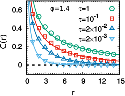
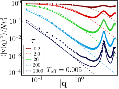
Figure 1: Left panel: velocity correlations for ABP systems studied in Refs. [33, 34] for different persistence times $\tau$ at $v_{0}=50$. Symbols: simulation results. Lines: theoretical predictions. Reprinted with Author’s permission from Ref. [34]. Right panel: velocity correlations for ABP systems studied in Ref. [13] for different persistence times $\tau$ at $T_{a}=0.005$. Dots: simulation results. Lines: theoretical predictions; solid line: normal mode-based approach; dashed lines: continuum elasticity approach. Reprinted with Author’s permission from Ref. [13].

In a recent work Caprini and Marconi [37] investigated underdamped analogues of active Brownian particles systems. They showed that long-ranged equal-time velocity correlations persist in the presence of inertia and thermal fluctuations. We note that Caporuso et al. [38] did not find long-ranged equal-time velocity correlations in overdamped systems of active Brownian particles with thermal fluctuations. We suggest that further work is needed to clarify these somewhat conflicting results.

3 Long-ranged velocity correlations in dense amorphous systems of self-propelled particles

Henkes et al. [13] completed a combined experimental, simulational and theoretical study of velocity correlations in active matter systems. On the experimental side they studied the dynamics of epithelial cell monolayers and found displacement and velocity correlations over several cell sizes. They found that the displacement correlations resembled those observed in supercooled liquids. Conversely, there are no equal-time velocity correlations in liquids.

Henkes et al. simulated $2d$ systems of repulsive polydisperse overdamped active Brownian particles. They also simulated systems of polydisperse self-propelled Voronoi cells [39, 40], which can be thought of as active objects with complicated many-particle (non-pairwise-additive) interactions. The polydispersity was introduced to account for cell size heterogeneity. As a result, systems simulated by Henkes et al. remained amorphous in the range of the parameters used in their study.

Henkes et al. found that non-trivial equal-time velocity correlations exist in both simulated systems. In agreement with the results obtained by Caprini et al., the range of these correlations was found to increase as the square-root of the persistence time of the self-propulsion.

To explain their results Henkes et al. assumed that on short enough time scales, their systems can be approximated by amorphous elastic solids. They used two related approaches. First, they generated local potential energy minima (inherent structures) corresponding to configurations obtained in simulations and approximated the real short-time dynamics by harmonic motion around these minima. They found the associated normal modes and expressed the equal-time velocity correlations in terms of normal mode frequencies, normal mode amplitudes and the persistence time. Second, Henkes et al. postulated a continuum elastic description of their active systems. In this case, the equal-time velocity correlations were expressed in terms of the elastic bulk and shear moduli, and the persistence time,

$$\left<|\mathbf{v}(\mathbf{q})|^{2}\right>=\frac{Nv_{0}^{2}}{2}\left[\frac{1}{1+\left(\xi_{L}q\right)^{2}}+\frac{1}{1+\left(\xi_{T}q\right)^{2}}\right]$$ (4)

where $\mathbf{v}(\mathbf{q})=\sum_{j}\dot{\mathbf{r}}_{j}e^{-i\mathbf{q}\cdot\mathbf{r}_{j}}$, $N$ is the number of particles, $v_{0}$ is the self-propulsion velocity. The correlation lengths $\xi_{L}$ and $\xi_{T}$ can be expressed in terms of the bulk $B$ and shear $\mu$ moduli as $\xi_{L}^{2}=\left(B+\mu\right)\tau/\gamma$ and $\xi_{T}^{2}=\mu\tau/\gamma$.

The normal mode-based approach gives quite accurate predictions for both small and large wavevectors, see the solid line in the right panel of Fig. 1. By construction, the continuum elastic approach is only applicable in the small wavevector (large distance) limit, and in this limit it reproduces the results of the normal mode approach, see the dashed lines in the right panel of Fig. 1.

While Henkes et al.’s approach is generally applicable to active systems exhibiting slow glassy-like dynamics, from a physical point of view it seems inapplicable to dense active systems with constituents moving perhaps slowly but in a standard, fluid-like fashion.

4 Long-ranged velocity correlations in dense fluid-like systems of self-propelled particles

We originally stumbled upon non-trivial equal-time velocity correlations when developing a theory for the dynamics of of active Ornstein-Uhlenbeck particles [41, 42, 43]. We found that these correlations determine their short-time dynamics [30, 31, 44, 45] and they also appear in an approximate mode-coupling-like theory for active particle systems [46].

Here we present computer simulation results showing that velocity correlations in dense active fluid-like systems are long-ranged. To rationalize this finding we develop a simple theory similar to the one presented by Henkes et al. Our theory does not assume elastic response, is applicable to fluid-like systems and describes the major part of the long-ranged velocity correlations.

4.1 Simulations

We simulated two-dimensional polydisperse systems of active Brownian particles [35, 36]. The equations of motion for the position $\mathbf{r}_{i}$ and the angle $\phi_{i}$ specifying the orientation of the self-propulsion of particle $i$ are given by

$$\gamma\dot{\mathbf{r}}_{i} = -\nabla_{i}\sum_{j}V(r_{ij})+\gamma v_{0}\mathbf{n}_{i}$$ (5)

$$\dot{\phi}_{i} = \eta_{i},$$ (6)

where $v_{0}$ is the self-propulsion velocity, $\mathbf{n}_{i}=(\cos(\phi_{i}),\sin(\phi_{i}))$ is the orientation vector specifying the direction of the self propulsion, and the random variable $\eta(t)$ satisfies $\left<\eta_{i}(t)\eta_{j}(t^{\prime})\right>=2D_{r}\delta_{ij}\delta(t-t^{\prime})$. In $2d$, persistence time of the self-propulsion, $\tau$, is the inverse of the rotational diffusion coefficient, $\tau=1/D_{r}$. For an isolated active particle, Eqs. (5-6) result in a mean-square displacement that for long times grows as $\left<\delta r^{2}(t)\right>\simeq\frac{2v_{o}^{2}}{D_{r}}t$. Comparing this result to the mean-square displacement of a Brownian particle in $2d$, $\left<\delta r^{2}(t)\right>=4T/\gamma$, we can define an active temperature $T_{a}=v_{0}^{2}\gamma/(2D_{r})$.

The interaction potential is given by

$$V(r_{ij})=\epsilon\left(\frac{\sigma_{ij}}{r_{ij}}\right)^{12}+c_{0}+c_{2}\left(\frac{r_{ij}}{\sigma_{ij}}\right)^{2}+c_{4}\left(\frac{r_{ij}}{\sigma_{ij}}\right)^{4},$$ (7)

when the distance between particles $i$ and $j$, $r_{ij}<1.25\sigma_{ij}$ and zero otherwise. In Equation 7 coefficients $c_{\alpha}$ are chosen so that the potential and the first two derivatives are continuous. The diameters $\sigma_{i}$ are chosen from the distribution $P(\sigma)=A/\sigma^{3}$ for $0.73<\sigma<1.63$. The cross diameter $\sigma_{ij}=0.5(\sigma_{i}+\sigma_{j})(1-0.2|\sigma_{i}-\sigma_{j}|)$. The number density is $\rho=1.23$. The interaction potential and the density are chosen to prevent crystallization and significant structural changes for a large range of simulation parameters.

Most of the simulations were done using $N=10000$ particles. Due to the long-range of the velocity correlations, the simulations for the three lowest $D_{r}$ used $N=250000$ particles.

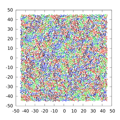
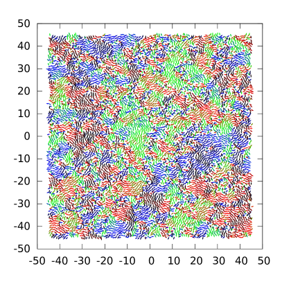
Figure 2: Snapshots of configurations for $\tau=0.14$ (left panel) and $\tau=10.0$ (right panel). Arrows show orientations of the velocities; specific velocity directions are also color-coded.

4.2 Velocity Correlations

Qualitatively, the increase of the range of velocity correlations is evident from snapshots shown in Fig. 2. To quantify these correlations we introduce two correlation functions. The first function,

$$\omega_{\parallel}(q)=\frac{1}{N}\left<\left|\hat{\mathbf{q}}\cdot\mathbf{v}(\mathbf{q})\right|^{2}\right>,$$ (8)

which we refer to as the longitudinal velocity correlation function, appeared naturally in the analysis of the short-time behavior of the intermediate scattering function of self-propelled particles [30]. Here we examine $\omega_{\parallel}(q)$ and the complementary part of velocity correlations, the transverse velocity correlation function,

$$\omega_{\perp}(q)=\frac{1}{N}\left<\left|\mathbf{v}(\mathbf{q})-\hat{\mathbf{q}}(\hat{\mathbf{q}}\cdot\mathbf{v}(\mathbf{q}))\right|^{2}\right>.$$ (9)

The wavevectors $\mathbf{q}$ in Eqs. (8-9) have to satisfy periodic boundary conditions. Both $\omega_{\parallel}(q)$ and $\omega_{\perp}(q)$ are equal to $v_{0}^{2}/2$ for $q=0$, which is useful in fits for the correlation length described below.

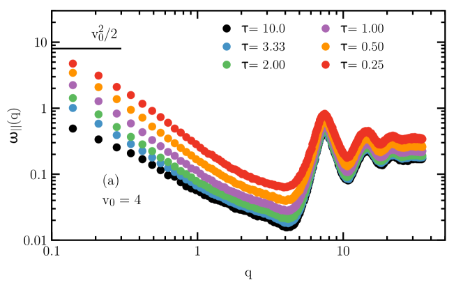
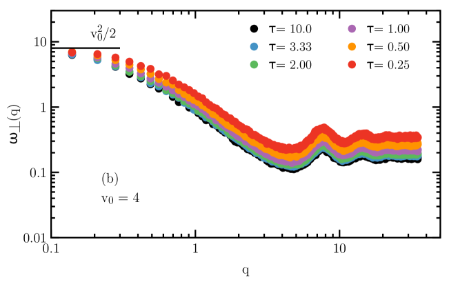
Figure 3: The equal time velocity correlation functions (a) $\omega_{\parallel}(q)$ and (b) $\omega_{\perp}(q)$ calculated at a fixed $v_{0}=4$ for a range of $\tau$. The longitudinal correlation function $\omega_{\parallel}(q)$ indicates a a correlation length rapidly growing with increasing $\tau$.

The large number of parameters, $v_{0}$, $D_{r}$, $\rho$, necessitates choosing some cuts through the parameter space. We note that Caprini et al. fixed $v_{0}$ and examined velocity correlations as a function of the persistence time $\tau=1/D_{r}$ for various densities whereas Henkes et al. fixed $\rho$ and examined velocity correlations as a function of $\tau$ for a fixed value of active temperature $T_{a}=v_{0}^{2}\gamma/D_{r}$ and as a function of $T_{a}$ for a fixed value of $\tau$. Here we fix $\rho=1.23$ and examine velocity correlations as a function of $\tau=1/D_{r}$, first for a fixed value of $v_{0}=4$ and then for a fixed value of $T_{a}=8$. One interesting feature of the latter procedure is that the system approaches a Brownian system with $T=T_{a}$ for $\tau\to 0$, and it has been argued that with increasing $\tau$ at fixed $T_{a}$ the active system moves systematically farther away from equilibrium [47].

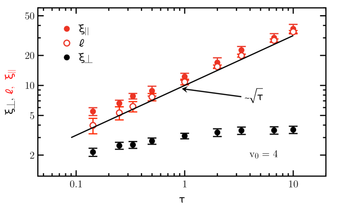
Figure 4: The longitudinal correlation length $\xi_{\parallel}$ obtained from fitting $\omega_{\parallel}(q)$ (filled red circles) and transverse correlation length $\xi_{\perp}$ (filled black circles) obtained from fitting $\omega_{\perp}(q)$ (closed black circles) for a fixed self-propulsion velocity $v_{0}=4$. The longitudinal correlation length grows approximately as $\sqrt{\tau}$, while the transverse correlation length is almost unchanged for a fixed $v_{0}$. The open red circles are results of the approximate theory.

In Fig. 3(a) we show $\omega_{\parallel}(q)$ for $v_{0}=4$ and a range of $\tau$ from 0.14 to 10. Since $\omega_{\parallel}(q=0)$ is constant for a fixed $v_{0}$, it is apparent that there is a faster decay of $\omega_{\parallel}(q)$ at the small wavelengths with increasing $\tau$, which corresponds to a longer range of longitudinal velocity correlations.

In contrast, $\omega_{\perp}(q)$, which is shown in Fig. 3(b) changes little with $\tau$, which implies that transverse velocity correlations are significantly less dependent on $\tau$ at fixed $v_{0}$.

To determine the velocity correlation length, we fitted $\omega_{\alpha}(q)$ for $q<0.2$ to an Ornstein-Zernike-like form $(v_{0}^{2}/2)/[1+(\xi_{\alpha}q)^{2}]+\omega_{\alpha}(\infty)$. In Fig. 4 we show correlation lengths $\xi_{\parallel}$ and $\xi_{\perp}$ obtained from fitting $\omega_{\parallel}(q)$ and $\omega_{\perp}(q)$, respectively. The longitudinal correlation length increases from approximately 4 at $\tau=0.14$ to 34 at $\tau=10.0$ whereas the transverse length increases only slightly over the full range of $\tau$.

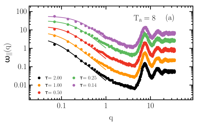
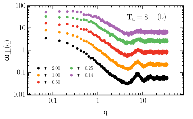
Figure 5: The equal time velocity correlation functions (a) $\omega_{\parallel}(q)$ and (b) $\omega_{\perp}(q)$ calculated at a fixed active temperature $T_{a}=8$ for a range of $\tau$. The longitudinal correlation function $\omega_{\parallel}(q)$ indicates a correlation length growing with increasing $\tau$. The transverse correlation function $\omega_{\perp}(q)$ also suggests a growing length scale, albeit a smaller one. Solid lines in (a) are predictions of the approximate theory, Eq. (16).

In Fig. 5 we show $\omega_{\parallel}(q)$ and $\omega_{\perp}(q)$ for a fixed $T_{a}=8$. Since increasing persistence time for a fixed value of the active temperature results in a rapidly slowing diffusive motion of the particles, we could only simulate a restricted range of $\tau$. Once again we observe increasing range of velocity correlations, but for fixed $T_{a}$ the range of both longitudinal and transverse correlations is increasing.

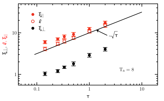
Figure 6: The longitudinal velocity correlation length $\xi_{\parallel}$ (filled red circles) and the transverse correlation length $\xi_{\perp}$ (filled black circles) for a fixed active temperature $T_{a}=8$. Solid lines in (a) represent theoretical predictions. The longitudinal correlation length is much larger than the transverse correlation length, but they both grow approximately as $\sqrt{\tau}$ for fixed $T_{a}$. The open red circles are predictions of the approximate theory.

We obtained velocity correlation lengths from fits to an Ornstein-Zernicke-like function and we present these lengths in Fig. 6. For large $\tau$ both correlation lengths grow with increasing persistence time. We recall that we did not observe growing $\xi_{\perp}$ at fixed $v_{0}$, which implies that this length must also depend on $v_{0}$.

4.3 Theory

Our starting point for an approximate theory for velocity correlations is equation of motion (5) from which we derive the following relation between velocity, polarization and force fields in the Fourier space,

$$\gamma\mathbf{v}(\mathbf{q};t)=\sum_{j}\sum_{k\neq j}\mathbf{F}_{jk}e^{-i\mathbf{q}\cdot\mathbf{r}_{j}}+\gamma v_{0}\mathbf{n}(\mathbf{q};t)$$ (10)

where $\mathbf{v}(\mathbf{q};t)=\sum_{j}\dot{\mathbf{r}}_{j}e^{-i\mathbf{q}\cdot\mathbf{r}_{j}(t)}$ and $\mathbf{n}(\mathbf{q};t)=\sum_{j}\mathbf{n}_{j}e^{-i\mathbf{q}\cdot\mathbf{r}_{j}(t)}$. Next, we follow Sec. 8.4 of Hansen and McDonald’s monograph [48] and we re-write the first term at the right-hand-side of Eq. (10) as

$$i\mathbf{q}\cdot\sum_{j}\sum_{k\neq j}\mathbf{r}_{jk}\frac{\mathbf{r}_{jk}}{2r_{jk}}V^{\prime}(r_{jk})\left[\frac{e^{i\mathbf{q}\cdot\mathbf{r}_{jk}}-1}{i\mathbf{q}\cdot\mathbf{r}_{jk}}\right]e^{-i\mathbf{q}\cdot\mathbf{r}_{j}}$$ (11)

$$= -i\mathbf{q}\cdot\mathbf{\Pi}_{v}(\mathbf{q};t),$$

where $\mathbf{r}_{jk}=\mathbf{r}_{j}-\mathbf{r}_{k}$ and $\mathbf{\Pi}_{v}$ has the same form as the virial (interaction) part of the pressure tensor. We then assume that in the direct space $\mathbf{\Pi}_{v}(\mathbf{r};t)$ can be expressed in terms of the instantaneous deviation of the density from its steady-state average value $\rho$,

$$\mathbf{\Pi}_{v}(\mathbf{r};t)\approx\left<\mathbf{\Pi}_{v}(\mathbf{r};t)\right>+\mathbf{I}\left(\partial_{\rho}P_{v}\right)\left(\rho(\mathbf{r};t)-\rho\right),$$ (12)

where $\mathbf{I}\left(\partial_{\rho}P_{v}\right)=\partial\left<\mathbf{\Pi}_{v}(\mathbf{r};t)\right>/\partial\rho$ and $\mathbf{I}$ is the unit tensor. In the steady state, averages $\left<\mathbf{\Pi}_{v}(\mathbf{r};t)\right>\equiv P_{v}$ and $\rho$ are translationally invariant. Thus, combining Eqs. (11) and (12) we obtain the following approximate expression for the first term at the right-hand-side of Eq. (10)

$$-i\mathbf{q}\left(\partial_{\rho}P_{v}\right)\sum_{j}e^{-i\mathbf{q}\cdot\mathbf{r}_{j}(t)}.$$ (13)

Next, we take a time derivative and Fourier transform in time and we obtain

$$-\gamma i\omega\mathbf{v}(\mathbf{q};\omega)\approx-\gamma v_{o}i\omega\mathbf{n}(\mathbf{q};\omega)-\mathbf{q}\left(\partial_{\rho}P_{v}\right)\mathbf{q}\cdot\mathbf{v}(\mathbf{q};\omega).$$ (14)

To proceed we choose $\mathbf{q}=(q,0)$, which allows us to write

$$v^{x}(\mathbf{q},\omega)=\frac{i\omega\gamma v_{0}n^{x}(\mathbf{q};\omega)}{\gamma i\omega-q^{2}(\partial_{\rho}P_{v})}$$ (15)

for the longitudinal correlations. Finally, using the same arguments as Henkes et al. [13], we obtain the equal-time longitudinal velocity correlations

$$\left<\left|\hat{\mathbf{q}}\cdot\mathbf{v}(\mathbf{q})\right|^{2}\right>=\frac{Nv_{0}^{2}}{2}\frac{1}{1+q^{2}\tau B_{v}/(\gamma\rho)}.$$ (16)

We identify correlation length $\xi_{\parallel}=\sqrt{\tau B_{v}/(\gamma\rho)}$ where $B_{v}=\rho\partial_{\rho}P_{v}$ is the virial bulk modulus of the active fluid.

We calculated virial bulk modulus $B_{v}$ for our active fluid, and found that it depends weakly on $\tau$. $B_{v}$ increases slightly from 136 for $\tau=0.14$ to 148 for $\tau=10.0$ at a fixed $v_{0}=4$ and in our range of persistence times it is approximately constant and equal to 145 at fixed $T_{a}=8$. The resulting dynamic correlation length is shown in Figs. 4 and 6 as open red symbols. The increase of the correlation length $\xi_{\parallel}$ is predominantly due to the increase of the persistence time for both fixed $v_{0}=4$ and fixed $T_{a}=8$. Our simple theory accurately captures almost all of $\xi_{\parallel}$, but it does not predict any transverse velocity correlations. More work is needed to understand these correlations in active fluids, as opposed to ordered and amorphous solids discussed in earlier studies.

4.4 Properties of our active system

In this section we briefly present some of the properties of our system and show that it remains a single-phase fluid in the range of the parameters that we investigated. First, we evaluated the pair-correlation function $g(r)=\frac{1}{\rho N}\left<\sum_{j}\sum_{k\neq j}\delta\left[\mathbf{r}-(\mathbf{r}_{j}-\mathbf{r}_{k})\right]\right>,$ which is sensitive to changes in the local structure and to fractionation that could occur in our polydisperse system. Parenthetically, the polydispersity results in significantly broader peaks in $g(r)$ compared to single-component systems. In Fig. 7(a) we show $g(r)$ for simulations with fixed $v_{0}=4$. We see very little change in the structure over the whole range of $\tau$. In general, the height of the first peak decreases slightly with increasing $\tau$. In Fig. 7(b) we show $g(r)$ for fixed $T_{a}=8$ and, again, we see little change from a liquid like structure. In this case, we find that the height of the first peak decreases with decreasing $\tau$. In both cases we do not see any indication of crystallization or fractionation.

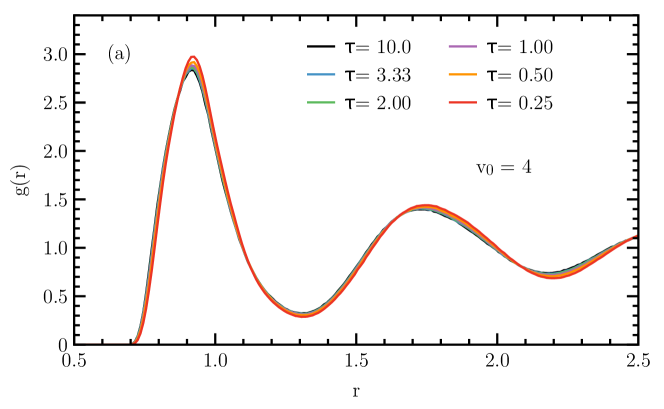
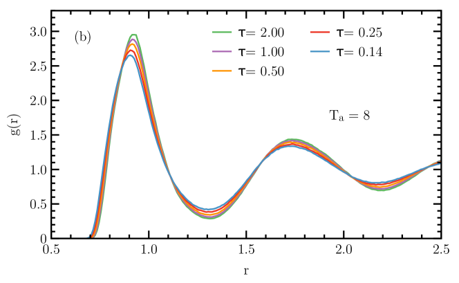
Figure 7: Pair correlation functions for (a) fixed $v_{0}=4$ and (b) fixed $T_{a}=8$. There is no significant change in the liquid structure over the full range of the simulation parameters.

To examine the dynamics of our system we evaluated mean square displacement $\left<\delta r^{2}(t)\right>=N^{-1}\left<\sum_{j}[\mathbf{r}_{j}(t)-\mathbf{r}_{j}(0)]^{2}\right>$. In Fig. 8 we show $\left<\delta r^{2}(t)\right>$ for the simulations with fixed $v_{0}=4$ (upper panel) and for simulations with fixed $T_{a}=8$ (lower panel). For both sets of parameters the long time motion is diffusive. However, the system monotonically speeds up with increasing $\tau$ for fixed $v_{0}=4$, while it monotonically slows down with increasing $\tau$ for fixed $T_{a}=8$. This behavior may be expected for fixed $v_{0}=4$ since the diffusion coefficient of an isolated particle for fixed $v_{0}$ grows as $\tau$. For small enough $\tau$ the system may approach a structural arrest, which would cause a dramatic slowing down, but we do not observe it in these simulations. For fixed $T_{a}$, on the basis of our earlier work on the dynamics of systems of self-propelled particles [44, 47], we would expect a non-monotonic dependence of the long-time diffusion on the persistence time but we did not simulated large enough range of $\tau$ to see it.

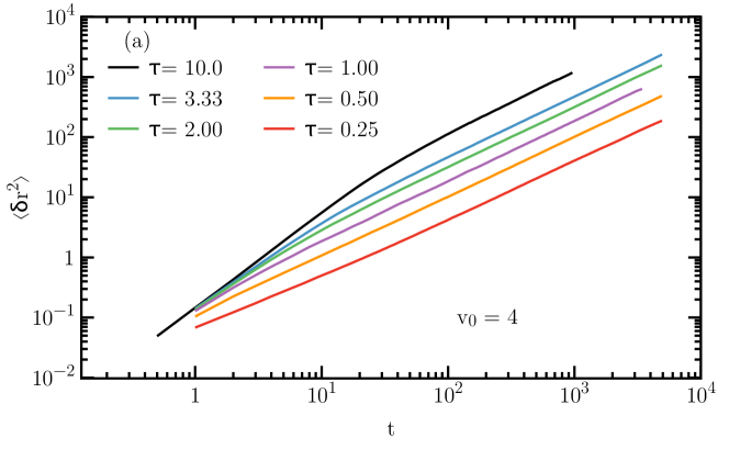
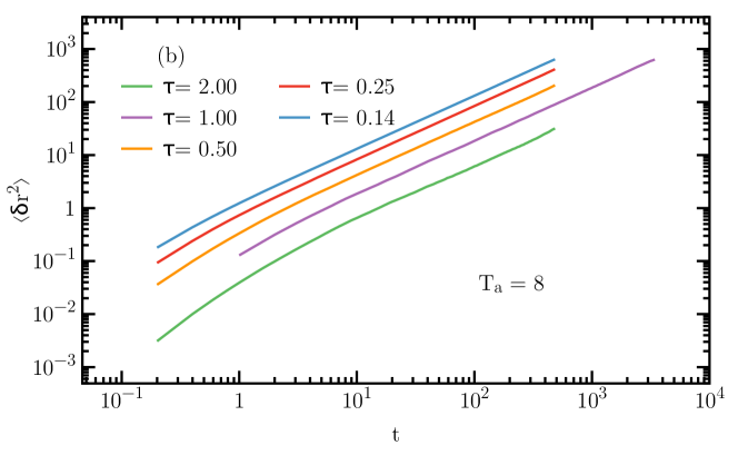
Figure 8: The mean-square displacement $\left<\delta r^{2}(t)\right>$ for (a) fixed $v_{0}=4$ and (b) fixed $T_{a}=8$ for the range of $\tau$ studied in this work. All the systems are diffusive at long times and they don’t show any signs of arrest or glassy dynamics. For a fixed $v_{0}=4$ increasing $\tau$ results in faster dynamics, while for a fixed $T_{a}=8$ increasing $\tau$ results in slower dynamics. Note that for $\tau=1.0$, $v_{0}=4$ and $T_{a}=8$ correspond to the same state point.

Finally, to check for macroscopic motility-induced phase separation and for the appearance of significant local density fluctuations we examined the probability distribution of the local density. To this end we divided the system into squares of length 10 and calculated the probability of the density for these squares. For a system that undergoes motility induced phase separation one should see this probability bifurcate into high density and low density. The local density probability distribution that we obtained exhibited a single peak only, indicating single phase, and generally changed little in the range of the parameters that we investigated.

5 Discussion

Equal-time velocity correlations are a ubiquitous feature of active matter systems, regardless of whether the system is arrested or diffusive and ordered or amorphous. These velocity correlations can be very long ranged for large persistence times. The correlations in the arrested (or almost arrested) systems can be rationalized in terms of the combined effect of the persistence of the directed motion and the elastic response of these systems. The longitudinal correlations in the diffusive systems can be explained in terms of the combined effect of the persistence and the fluid’s virial bulk modulus, which originates from repulsive interparticle interactions. The description of the transverse velocity correlations in diffusive systems that do not exhibit features of glassy dynamics is an open problem that deserves further study.

In our opinion, the most interesting open question is the relation of the long-ranged velocity correlations to the macroscopic properties of active matter. For example, active and passive systems with the same local structure, as examined by the pair distribution function or the static structure factor, usually have very different dynamic properties. Which of the differences can be attributed to the existence of equal-time velocity correlations in active matter systems? Are these differences sensitive to the range of the velocity correlations? We hope that this Letter will stimulate further work in this direction.

- [1] \NameRamaswamy S. \REVIEWAnn. Rev. Cond. Matt. Phys.12010323.
- [2] \NameVicsek T. Zafeiris A. \REVIEWPhys. Reports3-4201271.
- [3] \NameMarchetti M.C., Joanny J.F., Ramaswamy S., Liverpool T.B., Prost J., Rao M. Adit Simha R. \REVIEWRev. Mod. Phys.8520131143.
- [4] \NameElgeti J., Winkler R.G. Gompper G. \REVIEWRep. Prog. Phys.782015056601.
- [5] \NameBechinger C., Di Leonardo R., Löwen H., Reichhardt C., Volpe G. Volpe G. \REVIEWRev. Mod. Phys.882016045006.
- [6] \NameNeedleman D. Dogic Z. \REVIEWNat. Rev. Mat.2201717048
- [7] \NameGompper G., Winkler R.G., Speck T., Solon A., Nardini C., Peruani F., Löwen H. Golestanian R., Kaupp U.B., Alvarez L., et al. \REVIEWJ. of Phys.: Cond. Matt.322020193001
- [8] \NamePetitjean L., Reffay M., Grasland-Mongrain E., Paujade M., Ladoux B., Buguin A. Silberzan P. \REVIEWBiophysical J.9820101790.
- [9] \NameAngelini T.E., Hannezo E., Trepat X., Marques M., Fredberg J.J, and Weitz D.A. \REVIEWPNAS10820114714.
- [10] \NameBasan M., Elgeti J., Hannezo E., Rappel W.-J. Levine H. \REVIEWPNAS11020132452.
- [11] \NameGarcia S., Hannezo E., Elgeti J., Joanny J.-F., Silberzan P. Gav N.S. \REVIEWPNAS112201515314.
- [12] \NameBlanch-Mercader C., Yashunsky V., Garcia S., Duclos G., Giomi L. Silberzan P. \REVIEWPhys. Rev. Lett.1202018208101.
- [13] \NameHenkes S., Kostanjevec K., Collinson J.M., Sknepnek R. Bertin E. \REVIEWNat. Commun.1120201.
- [14] \NameDombrowski C., Cisneros L., Chatkaew S., Goldstein R.E. Kessler J.O. \REVIEWPhys. Rev. Lett.932004098102.
- [15] \NamePeruani F., Starruss J., Jakovljevic V., Sogaard-Andersen L., Deutsch A. Bär M. \REVIEWPhys. Rev. Lett.1082012098102.
- [16] \NameWensink H.H., Dunkel J., Heidenreich S., Drescher K., Goldstein R.E., Löwen H. Yeomans J.M. \REVIEWPNAS109201214308.
- [17] \NameDunkel J., Heidenreich S., Drescher K., Wensink H.H., Bär M., Goldstein R.E. \REVIEWPhys. Rev. Lett.1102013228102.
- [18] \NameWioland H., Woodhouse F.G., Dunkel J., Goldstein R.E. \REVIEWNat. Phys.122016341.
- [19] \NameUrzay J., Doostmohammadi A. Yeomans J. \REVIEWJ. Fluid Mech.8222017762
- [20] \NameJames M., Bos W.J. Wilczek M. \REVIEWPhys. Rev. Fluids32018061101.
- [21] \NameHowse J.R., Jones R.A.L., Ryan A.J., Gough T., Vafabakhsh R. Golestanian R. \REVIEWPhys. Rev. Lett.992007048102.
- [22] \NameTierno P., Golestanian R., Paganabarraga I. Sagués F. \REVIEWJ. Phys. Chem. B112200816525.
- [23] \NameGosh A. Fischer P. \REVIEWNano Lett.920092243.
- [24] \NamePalacci J., Cottin-Bizonne C., Ybert C. Bocquet L. \REVIEWPhys. Rev. Lett.1052010088304.
- [25] \NameJiang H.R., Yoshinaga N. Sano M. \REVIEWPhys. Rev. Lett.1052010268302.
- [26] \NameMichelin S., Lauga E. Bartolo D. \REVIEWPhys. Fluids252013061701.
- [27] \NameDai B., Wang J., Xiong Z., Zhan X., Dai W., Li C.-C., Feng S.-P. Tang J. \REVIEWNature Nano.1120161087.
- [28] \NameMoran J. L. Posner J.D. \REVIEWAnnu. Rev. Fluid Mech.492017511.
- [29] \NameCates M.E. Tailleur J. \REVIEWAnn. Rev. Cond. Matt. Phys.62015219.
- [30] \NameSzamel G., Flenner E. Berthier L. \REVIEWPhys. Rev. E912015062304.
- [31] \NameFlenner E., Szamel G. Berthier L. \REVIEWSoft Matter1220167136.
- [32] \NameMarconi U.M.B., Gnan N., Paoluzzi M., Maggi C. Di Leonardo R. \REVIEWSci. Rep.6201623297.
- [33] \NameCaprini L., Marconi U.M.B. Puglisi A. \REVIEWPhys. Rev. Lett.1242020078001.
- [34] \NameCaprini L., Marconi U.M.B, Maggi C., Paoluzzi P. Puglisi A. \REVIEWPhys. Rev. Res.22020023321.
- [35] \Nameten Hagen B., van Teeffelen A. H. Löwen \REVIEWJ. Phys.: Condens. Matter232011194119.
- [36] \NameFily Y. Marchetti M.C. \REVIEWPhys. Rev. Lett.1082012235702.
- [37] \NameCaprini L. Marconi U.M.B. \ReviewarXiv:2012.11916.
- [38] \NameCaporusso C.B., Digregorio P., Levis D., Cugliandolo L.F. Gonnella G. \REVIEWPhys. Rev. Lett.1252020178004.
- [39] \NameBi, D., Yang, X., Marchetti, M. C. Manning, M. L. \REVIEWPhys. Rev. X6201621011.
- [40] \NameBarton, D. L., Henkes, S., Weijer, C. J. Sknepnek, R. \REVIEWPLoS Comput. Biol.132017e1005569.
- [41] \NameSzamel G. \REVIEWPhys. Rev. E902014012111.
- [42] \NameMaggi C., Marconi U.M.B., Gnan N. Di Leonardo R. \REVIEWSci. Rep.5201510742.
- [43] \NameFodor E., Nardini C., Cates M.E., Tailleur J., Visco P., van Wijland F. \REVIEWPhys. Rev. Lett.1172016038103.
- [44] \NameBerthier L., Flenner E. Szamel G. \REVIEWNew J. Phys.192017125006.
- [45] \NameBerthier L., Flenner E. Szamel G. \REVIEWJ. Chem. Phys.1502019200901.
- [46] \NameSzamel G. \REVIEWPhys. Rev. E932016012603.
- [47] \NameE. Flenner G. Szamel \REVIEWPhys. Rev. E1022020022605.
- [48] \NameHansen, J.-P. McDonald, I.R. \BookTheory of Simple Liquids, 4th Ed. \PublAcademic, London \Year2013.