Tripartite Entanglement of Hawking Radiation in Dispersive Model

Abstract

We investigate entanglement of the Hawking radiation in a dispersive model with subluminal dispersion. In this model, feature of the Hawking radiation is represented by three mode Bogoliubov transformation connecting the in-vacuum state and the out-state. We obtain the exact form of the tripartite in-vacuum state which encodes structure of multipartite entanglement. Bogoliubov coefficients are computed by numerical calculation of the wave equation with subluminal dispersion and it is found that genuine tripartite entanglement persists in whole frequency range up to the cutoff arisen from the subluminal dispersion. In the low frequency region, amount of the tripartite entanglement is far small compared to bipartite entanglement between the Hawking particle and its partner mode, and the deviation from the thermal spectrum is negligible. On the other hand, in the high frequency region near the cutoff, entanglement of the system is equally shared by two pairs of three modes, and the thermal nature of the Hawking radiation is lost.

I Introduction

The black hole horizon causes an extremely large redshift on outgoing waves propagating from the vicinity of the horizon to the asymptotically flat region. This redshift results in the Planckian distribution of quantum mechanically created Hawking radiation Hawking1974 ; Hawking1975a . The original Hawking’s scenario relies on the assumption of infinite amount of modes whose wavelength is shorter than the Planck scale. Thus there is a possibility that sub-Planckian physics alter the nature of the Hawking radiation (trans-Planckian problem). Within a setup of analog models of black hole geometry using moving media with high frequency cutoff, the issue of the trans-Planckian problem has been investigated by many researchers Unruh1995a ; Brout1995a ; Corley1996a ; Tanaka2000a ; Jacobson2003 ; Unruh2005a ; Macher2009 ; Macher2009b ; Robertson2012 ; Leonhardt2012 ; Coutant2012 . The main purpose of these works is to clarify the effect of high frequency cutoff on sub-Plankian origin of the thermal radiation predicted by the original Hawking’s work. These investigations show the robustness of the thermal nature of the Hawking radiation; deviation from the Planckian distribution of the Hawking radiation is small if the cutoff scale is much higher than the surface gravity scale which is determined by the gradient of the flow velocity at the sonic point.

The thermal nature of the Hawking radiation can be understood from a viewpoint of quantum correlation between the Hawking particles (Hawking radiation) and their entangled partners which fall into the black hole Hotta2015 . To verify the analog Hawking radiation in laboratory experiments, it is crucial to understand the entanglement structure of quasi-particles, of which excitation is observable by experiments to confirm the quantum nature of the Hawking effect. Considering excitation of quasi-particles in dispersive media, due to non-linear dispersion relation, new wave modes participate and they are responsible for forming multipartite entanglement structure of the Hawking radiation. Actually, even for $(1+1)$-dimensional models, right moving modes and left moving modes can mix each other and the Bogoliubov transformation between the in-modes and the out-modes becomes transformation between three modes Macher2009 ; Macher2009b ; Busch2014 . Behavior of entanglement involving three modes is investigated previously by Busch2014 for the purpose of distinguishing quantum signals of the Hawking radiation from classical thermal noise in laboratory experiments. Based on inequalities for correlations between each mode, which are equivalent to the Peres-Horodecki separability criterion Peres1996 ; Horodecki1997 ; Simon2000 , they analyzed separability of specified two modes. The separability is related to domination of stimulated emission due to the initial thermal state in the frame of fluid over spontaneous one, and they investigated parameter range of which the spontaneous emission is possible.

The three mode Bogoliubov transformation naturally leads to formation of multipartite entanglement among involving modes. The purpose of this paper is to clarify the structure of the multipartite entanglement of the Hawking radiation in dispersive media. We obtain the exact form of the in-vacuum state with three modes and examine entanglement between modes including the Hawking radiation. The plan of this paper is as follows. In Sec. II, we shortly review the Hawking radiation in dispersive models. In Sec. III, structure of the in-vacuum state involving three modes is clarified and entanglement structure of this state is investigated. In Sec. IV, we numerically solve the wave equation with subluminal dispersion and obtain the Bogoliubov coefficients which are required to determine the entanglement structure of three mode state. Sec. V is devoted to summary and conclusion. We adopt units $c=\hbar=G=1$ throughout this paper.

II Hawking radiation in dispersive model

We shortly review the Hawking radiation in a moving media with subluminal dispersion. This part is mainly based on articles Corley1996a ; Jacobson2003 ; Macher2009 ; Macher2009b ; Robertson2012 . The wave propagation in the media with stationary flow is governed by the following wave equation for scalar fluctuations (e.g. phonon)

$$(\partial_{t}+\partial_{x}V)(\partial_{t}+V\partial_{x})\phi=-F^{2}(-i\partial_{x})\phi,$$ (1)

where $V(x)$ denotes the background flow velocity and $F(-i\partial_{x})$ represents nonlinear modification of dispersion relation. The wave equation (1) is the specific case of the equations for sound waves in the perfect fluid obtained by assuming constant background density and constant sound velocity of the fluid. In general, the wave equation in fluid is not conformally invariant Anderson2014 ; Anderson2015 ; Fabbri2016 ; after separating time dependence, the wave equation can be written in the form of one dimensional Schrödinger equation with non-zero effective potential which originated from spatially dependent density and sound velocity. The non-zero effective potential causes mixing of right moving waves and left moving waves hence grey-body factors are nonzero. For the specific wave equation (1) adopted in this paper, the conformal invariance is violated due to dispersion and mixing of right moving waves and left moving waves occurs. The conformal invariance is recovered in the low frequency limit which corresponds to the dispersionless limit. As we will see, this mixing results in the tripartite entanglement of the Hawking radiation in dispersive models.

The velocity profile is assumed to be

$$V(x)=-1+D\tanh\left(\frac{\kappa x}{D}\right),\quad D<1.$$ (2)

The sonic horizon is located at $x=0$ for this flow (Fig. 1). The parameter $\kappa$ represents gradient of the flow velocity at the sonic horizon. The asymptotic flow velocity is $V_{+}:=V|_{x=+\infty}=-1+D,V_{-}:=V|_{x=-\infty}=-1-D$.

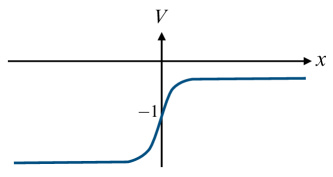
Figure 1: The profile of the background flow. The sonic horizon is located at $x=0$. For $x>0$, $|V|<1$ (subsonic) and for $x<0$, $|V|>1$ (supersonic).

As the flow is stationary, time dependence of the wave is separated as $\phi\propto e^{-i\omega t}$ and the wave equation becomes

$$(-i\omega+\partial_{x}V)(-i\omega+V\partial_{x})\phi=-F^{2}(-i\partial_{x})\phi.$$ (3)

The dispersion relation is obtained by substituting $\phi\propto e^{ikx}$:

$$(\omega-V\,k)^{2}=F(k)^{2},\quad F(k)=(k^{2}-k^{4}/k_{0}^{2})^{1/2},$$ (4)

where subluminal type of dispersion is assumed. The parameter $k_{0}$ determines the high frequency cutoff of the dispersion. It is possible to identify wave modes as solutions of Eq. (4) (Fig. 2). In the subsonic region $x>0$, there are two roots with negative wave numbers $k_{\bar{u}}(\omega),k_{v}(\omega)$, and two roots with positive wave numbers $k_{u_{1}}(\omega),k_{u_{2}}(\omega)$. In the supersonic region $x<0$, there are two modes with negative wave number $k_{\bar{u}}(\omega),k_{v}(\omega)$. These four roots represent modes appear in this model. We denote them as $u_{1},u_{2},\bar{u},v$. In the asymptotic region where $V(x)$ is constant, these modes behave as plane waves

$$\varphi_{m}(x)\sim e^{ik_{m}(\omega)x},\quad m=u_{1},u_{2},\bar{u},v.$$ (5)

The group velocity of each mode is

$$V_{g}=V(x)\pm F^{\prime}(k_{m}(\omega)).$$ (6)

The mode $u_{1}$ has positive group velocity (right moving) and the modes $u_{2},v,\bar{u}$ have negative group velocities (left moving).

Figure 2: Modes appear in this model. Left panel: supersonic region ($V<-1$), right panel: subsonic region ($-1<V<0$). Only $u_{1}$ mode is right moving. $\bar{u}$ mode corresponds to particles with negative energy (negative norm).

In the asymptotic subsonic region $x\rightarrow\infty$ where the flow velocity becomes constant, we introduce the cutoff frequency given by

$$\omega_{\text{cutoff}}=\frac{k_{0}}{16}\left(3V_{+}+\sqrt{V_{+}^{2}+8}\right)\left(8-2V_{+}^{2}+2V_{+}\sqrt{V_{+}^{2}+8}\right)^{1/2}.$$ (7)

For $\omega>\omega_{\text{cutoff}}$, the dispersion relation does not have real solutions with $k>0$ and there is no right propagating wave modes in the asymptotic region of $x>0$.

Spacetime trajectories of each mode are obtained by equations of motion derived from the Hamiltonian $\omega(k,x)$ (Fig. 3):

$$\frac{dx}{dt}=\frac{\partial\omega}{\partial k},\quad\frac{dk}{dt}=-\frac{\partial\omega}{\partial x},\quad\omega=V(x)\,k\pm F(k).$$ (8)

In the vicinity of the sonic horizon, the group velocity of the left moving mode $u_{2}$ becomes zero. At this point, the mode $u_{2}$ is reflected and converted to become the right moving $u_{1}$ mode. The location of the turning point depends on the cutoff frequency $\omega_{\text{cutoff}}$. Under the assumption that $|V_{+}|\ll 1$ and $\omega/\omega_{\text{cutoff}}\ll 1$, it is given by

$$\kappa x\approx\frac{3}{2}\left(\frac{\omega}{2\omega_{\text{cutoff}}}\right)^{2/3},$$ (9)

and as the cutoff frequency becomes larger, the turning point approaches the sonic horizon.

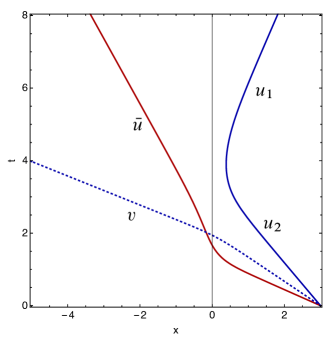
Figure 3: Left panel: schematic picture of modes in this model. We have three modes for the in-state and three modes for the out-state. Right panel: trajectories of each mode obtained by the Hamiltonian $\omega(k,x)$. In this figure, adopted parameters are $D=1/2,\kappa=1,k_{0}=1,\omega=0.10$. The left moving $u_{2}$ mode is reflected to become the right moving $u_{1}$ mode.

Let us introduce normalized wave modes $\varphi_{u_{1,2}}(\omega)\propto e^{-i\omega t},\varphi_{v}(\omega)\propto e^{-i\omega t},\varphi_{\bar{u}}(-\omega)\propto e^{i\omega t}$ with $\omega>0$. They are solutions of (1) and are orthogonal and normalized with respect to the Klein-Gordon inner product

$$(f,g):=i\int dx(f^{*}(\partial_{t}+V\partial_{x})g-g(\partial_{t}+V\partial_{x})f^{*}),$$ (10)

$$(\varphi_{u_{1,2}}(\omega_{1}),\varphi_{u_{1,2}}(\omega_{2}))=(\varphi_{v}(\omega_{1}),\varphi_{v}(\omega_{2}))=\delta(\omega_{1}-\omega_{2}),$$ (11)

$$(\varphi_{\bar{u}}(-\omega_{1}),\varphi_{\bar{u}}(-\omega_{2}))=-\delta(\omega_{1}-\omega_{2}).$$ (12)

The mode $\bar{u}$ has negative energy and negative norm. Now we consider the self-adjoint field operator $\hat{\phi}$ satisfying (1). The creation and annihilation operators associated with the mode $f$ of the wave equation (1) is defined by

$$\hat{a}(f)=(f,\hat{\phi}),\quad\hat{a}^{\dagger}(f)=-(f^{*},\hat{\phi}),$$ (13)

and they are independent of choice of the time slice. With the other solution $g$ of the wave equation, they satisfy

$$[\hat{a}(f),\hat{a}^{\dagger}(g)]=(f,g),\quad[\hat{a}(f),\hat{a}(g)]=-(f,g^{*}),\quad[\hat{a}^{\dagger}(f),\hat{a}^{\dagger}(g)]=-(f^{*},g).$$ (14)

The Hawking radiation in this model is explained as follows. As the in-state, we prepare the vacuum state,

$$\hat{a}(\varphi_{u}^{\text{in}})\ket{0_{\text{in}}}=\hat{a}(\varphi_{\bar{u}}^{\text{in}}{}^{*})\ket{0_{\text{in}}}=\hat{a}(\varphi_{v}^{\text{in}})\ket{0_{\text{in}}}=0.$$ (15)

Then, using the Bogoliubov transformation (19) which connects the in-out creation and annihilation operators, number of the out-state particle in the subsonic region is

$$\bra{0_{\text{in}}}\hat{a}^{\dagger}(\varphi^{\text{out}}_{u})\hat{a}(\varphi^{\text{out}}_{u})\ket{0_{\text{in}}} =|\alpha_{\bar{u}u}|^{2}\bra{0_{\text{in}}}\hat{a}(\varphi^{\text{in}}_{\bar{u}}{}^{*})\hat{a}^{\dagger}(\varphi^{\text{in}}_{\bar{u}}{}^{*})\ket{0_{\text{in}}}$$

$$=|\alpha_{\bar{u}u}|^{2}\bra{0_{\text{in}}}[\hat{a}(\varphi^{\text{in}}_{\bar{u}}{}^{*}),\hat{a}^{\dagger}(\varphi^{\text{in}}_{\bar{u}}{}^{*})]\ket{0_{\text{in}}}$$

$$=-|\alpha_{\bar{u}u}|^{2}(\varphi^{\text{in}}_{\bar{u}},\varphi^{\text{in}}_{\bar{u}})>0.$$ (16)

Nonzero particle number implies outgoing radiation from the sonic horizon. Previous works on the Hawking radiation in dispersive media predict the thermal spectrum of emitted particles with the Hawking temperature determined by the “surface gravity” $\kappa$, which corresponds to the gradient of the background flow velocity at the sonic horizon Unruh2005a .

III Structure of three mode in-vacuum state

We investigate structure of the in-vacuum state involving three modes which encode property of the Hawking radiation in dispersive models.

III.1 Three mode Bogoliubov transformation

Using the normalized modes $\varphi_{u},\varphi_{\bar{u}},\varphi_{v}$, the field operator is expressed as the Fourier expansion with respect to $\omega$ as

$$\hat{\phi}=\int_{0}^{\infty}d\omega\left(\hat{\phi}(\omega)e^{-i\omega t}+\hat{\phi}^{\dagger}(\omega)e^{i\omega t}\right),$$ (17)

where the Fourier component of the field operator is expressed as  Macher2009 ; Macher2009b ; Busch2014

$$\hat{\phi}(\omega) =\hat{a}_{u}^{\text{out}}(\omega)\varphi_{u}^{\text{out}}(\omega)+\hat{a}_{\bar{u}}^{\text{out}}{}^{{\dagger}}(-\omega)\left(\varphi_{\bar{u}}^{\text{out}}(-\omega)\right)^{*}+\hat{a}_{v}^{\text{out}}(\omega)\,\varphi_{v}^{\text{out}}(\omega)$$

$$=\hat{a}_{u}^{\text{in}}(\omega)\varphi_{u}^{\text{in}}(\omega)+\hat{a}_{\bar{u}}^{\text{in}}{}^{{\dagger}}(-\omega)\left(\varphi_{\bar{u}}^{\text{in}}(-\omega)\right)^{*}+\hat{a}_{v}^{\text{in}}(\omega)\,\varphi_{v}^{\text{in}}(\omega).$$ (18)

Creation and annihilation operators $\hat{a}_{j}^{\text{out}},\hat{a}_{j}^{\text{out}}{}^{\dagger}$ are associated with the out-state and $\hat{a}^{\text{in}}_{j},\hat{a}^{\text{in}}_{j}{}^{\dagger}$ are associated with the in-state where indices are $j=\{u,\bar{u},v\}$. From now on, we omit the argument $\omega$ of operators to simplify notations. Operators $\hat{a}_{j}^{\text{in,out}},\hat{a}_{j}^{\text{in,out}}{}^{\dagger}$ are related by the following three mode Bogoliubov transformation

$$\begin{bmatrix}\hat{a}_{u}^{\text{in}}\\ \hat{a}_{\bar{u}}^{\text{in}}{}^{\dagger}\\ \hat{a}_{v}^{\text{in}}\end{bmatrix}=\begin{bmatrix}\alpha_{uu}&\alpha_{u\bar{u}}&\alpha_{uv}\\ \alpha_{\bar{u}u}&\alpha_{\bar{u}\bar{u}}&\alpha_{\bar{u}v}\\ \alpha_{vu}&\alpha_{v\bar{u}}&\alpha_{vv}\end{bmatrix}\begin{bmatrix}\hat{a}_{u}^{\text{out}}\\ \hat{a}_{\bar{u}}^{\text{out}}{}^{\dagger}\\ \hat{a}_{v}^{\text{out}}\end{bmatrix}.$$ (19)

If the mixing between $u,\bar{u}$ and $v$ is negligible $\alpha_{uv}=\alpha_{\bar{u}v}=\alpha_{vu}=\alpha_{v\bar{u}}=0$, the transformation reduces to the two mode transformation which appears in standard calculations of the Hawking radiation. This mixing results in the gray-body factor in the power spectrum of the Hawking radiation. For $\hat{\mathcal{A}}^{\text{in,out}}:=(\hat{a}^{\text{in,out}}_{u},\hat{a}_{\bar{u}}^{\dagger}{}^{\text{in,out}},\hat{a}_{v}^{\text{in,out}})^{T}$, commutation relations between creation and annihilation operators can be written as $[\hat{\mathcal{A}}_{i}^{\text{in}},\hat{\mathcal{A}}_{j}^{\text{in}}{}^{\dagger}]=[\hat{\mathcal{A}}_{i}^{\text{out}},\hat{\mathcal{A}}_{j}^{\text{out}}{}^{\dagger}]=\eta_{ij}$ where $\eta_{ij}:=\mathrm{diag}(1,-1,1)$, and the Bogoliubov coefficients obey the following skew-unitarity relation Recati2009 :

$$\mathcal{S}\,\eta\,\mathcal{S}^{\dagger}=\eta,\quad\mathcal{S}:=\begin{bmatrix}\alpha_{uu}&\alpha_{\bar{u}u}&\alpha_{vu}\\ \alpha_{u\bar{u}}&\alpha_{\bar{u}\bar{u}}&\alpha_{v\bar{u}}\\ \alpha_{uv}&\alpha_{\bar{u}v}&\alpha_{vv}\end{bmatrix},\quad\hat{\mathcal{A}}^{\text{in}}=\mathcal{S}^{T}\hat{\mathcal{A}}^{\text{out}}.$$ (20)

This relation yields

$$|\alpha_{11}|^{2}-|\alpha_{12}|^{2}+|\alpha_{13}|^{2}=1,\quad-|\alpha_{21}|^{2}+|\alpha_{22}|^{2}-|\alpha_{23}|^{2}=1,$$

$$|\alpha_{31}|^{2}-|\alpha_{32}|^{2}+|\alpha_{33}|^{2}=1,$$ (21)

$$\alpha_{11}\,\alpha_{21}^{*}-\alpha_{12}\,\alpha_{22}^{*}+\alpha_{13}\,\alpha_{23}^{*}=0,\quad-\alpha_{21}^{*}\,\alpha_{31}+\alpha_{22}^{*}\,\alpha_{32}-\alpha_{23}^{*}\,\alpha_{33}=0,$$

$$\alpha_{11}\alpha_{31}{}^{\!\!\!*}-\alpha_{12}\alpha_{32}{}^{\!\!\!*}+\alpha_{13}\alpha_{33}{}^{\!\!\!*}=0,$$ (22)

$$|\alpha_{11}|^{2}-|\alpha_{21}|^{2}+|\alpha_{31}|^{2}=1,\quad-|\alpha_{12}|^{2}+|\alpha_{22}|^{2}-|\alpha_{32}|^{2}=1,$$

$$|\alpha_{13}|^{2}-|\alpha_{23}|^{2}+|\alpha_{33}|^{2}=1,$$ (23)

$$-\alpha_{11}{}^{\!\!\!*}\alpha_{12}+\alpha_{21}^{*}\alpha_{22}-\alpha_{31}{}^{\!\!\!*}\alpha_{32}=0,\quad\alpha_{12}\alpha_{13}{}^{\!\!\!*}-\alpha_{22}\alpha_{23}^{*}+\alpha_{32}\alpha_{33}{}^{\!\!\!*}=0,$$

$$\alpha_{11}\alpha_{13}{}^{\!\!\!*}-\alpha_{21}^{*}\alpha_{23}+\alpha_{31}{}^{\!\!\!*}\alpha_{33}=0,$$ (24)

where we adopted indices $\{1,2,3\}=\{u,\bar{u},v\}$. These equations are used to check accuracy of our numerical solutions of the wave equation. From the representation of the field operator

$$\hat{\phi}=\sum_{j}\hat{\mathcal{A}}^{\text{in}}_{j}\Phi^{\text{in}}_{j}=\sum_{j}\hat{\mathcal{A}}^{\text{out}}_{j}\Phi^{\text{out}}_{j},\quad\Phi^{\text{in,out}}:=(\varphi^{\text{in,out}}_{u},\varphi_{\bar{u}}^{*}{}^{\text{in,out}},\varphi_{v}^{\text{in,out}})^{T},$$ (25)

the in-mode functions and the out-mode functions are connected by $\Phi^{\text{out}}=\mathcal{S}\Phi^{\text{in}}$:

$$\begin{bmatrix}\varphi_{u}^{\text{out}}\\ \varphi_{\bar{u}}^{*}{}^{\text{out}}\\ \varphi_{v}^{\text{out}}\end{bmatrix}=\begin{bmatrix}\alpha_{uu}&\alpha_{\bar{u}u}&\alpha_{vu}\\ \alpha_{u\bar{u}}&\alpha_{\bar{u}\bar{u}}&\alpha_{v\bar{u}}\\ \alpha_{uv}&\alpha_{\bar{u}v}&\alpha_{vv}\end{bmatrix}\begin{bmatrix}\varphi_{u}^{\text{in}}\\ \varphi_{\bar{u}}^{*}{}^{\text{in}}\\ \varphi_{v}^{\text{in}}\end{bmatrix}.$$ (26)

III.2 In-vacuum state

We adopt the following parametrization of $\alpha_{\bar{u}u},\alpha_{\bar{u}\bar{u}},\alpha_{\bar{u}v}$ which satisfies $|\alpha_{\bar{u}\bar{u}}|^{2}-|\alpha_{\bar{u}u}|^{2}-|\alpha_{\bar{u}v}|^{2}=1$:

$$\alpha_{\bar{u}u}=e^{i\varphi_{1}}\cos\theta\sinh r,\quad\alpha_{\bar{u}\bar{u}}=e^{i\varphi_{2}}\cosh r,\quad\alpha_{\bar{u}v}=e^{i\varphi_{3}}\sin\theta\sinh r,\quad r\geq 0.$$ (27)

From linear combinations of $\hat{a}_{u}^{\text{out}},\hat{a}_{v}^{\text{out}}$, we introduce new annihilation operators $\hat{A}_{1},\hat{A}_{3}$ as

$$\hat{A}_{1}=e^{-i(\varphi_{1}-\varphi_{2})}\cos\theta\,\hat{a}_{u}^{\text{out}}+e^{-i(\varphi_{3}-\varphi_{2})}\sin\theta\,\hat{a}_{v}^{\text{out}},$$

$$\hat{A}_{3}=e^{i\varphi_{3}}\sin\theta\,\hat{a}_{u}^{\text{out}}-e^{i\varphi_{1}}\cos\theta\,\hat{a}_{v}^{\text{out}},\quad\hat{A}_{2}=\hat{a}_{\bar{u}}^{\text{out}}.$$ (28)

They satisfy $[\hat{A}_{i},\hat{A}_{j}{}^{\!{\dagger}}]=\delta_{ij},[\hat{A}_{i},\hat{A}_{j}]=0$. Inverting the relation,

$$\hat{a}_{u}^{\text{out}}=e^{i(\varphi_{1}-\varphi_{2})}\cos\theta\,\hat{A}_{1}+e^{-i\varphi_{3}}\sin\theta\,\hat{A}_{3},$$

$$\hat{a}_{v}^{\text{out}}=e^{i(\varphi_{3}-\varphi_{2})}\sin\theta\,\hat{A}_{1}-e^{-i\varphi_{1}}\cos\theta\,\hat{A}_{3},\quad\hat{a}_{\bar{u}}^{\text{out}}=\hat{A}_{2}.$$ (29)

By expressing the Bogoliubov transformation (19) in terms of new annihilation operators $\hat{A}_{j}$, we obtain

$$\hat{a}_{u}^{\text{in}}=\frac{\alpha_{u\bar{u}}}{\tanh r}\left(\hat{A}_{1}+\tanh r\hat{A}_{2}{}^{\!\!{\dagger}}\right)+(\alpha_{uu}e^{-i\varphi_{3}}\sin\theta-\alpha_{uv}e^{-i\varphi_{1}}\cos\theta)\hat{A}_{3},$$ (30)

$$\hat{a}_{\bar{u}}^{\text{in}}=\alpha_{\bar{u}\bar{u}}^{*}\left(\tanh r\hat{A}_{1}{}^{\!\!{\dagger}}+\hat{A}_{2}\right),$$ (31)

$$\hat{a}_{v}^{\text{in}}=\frac{\alpha_{v\bar{u}}}{\tanh r}\left(\hat{A}_{1}+\tanh r\hat{A}_{2}{}^{\!\!{\dagger}}\right)+(\alpha_{vu}e^{-i\varphi_{3}}\sin\theta-\alpha_{v\bar{u}}e^{-i\varphi_{1}}\cos\theta)\hat{A}_{3},$$ (32)

where we have used the relation $\alpha_{11}\alpha_{21}^{*}-\alpha_{12}\alpha_{22}^{*}+\alpha_{13}\alpha_{23}^{*}=0$. As the in-vacuum state $\ket{\psi_{0}}$ is determined by $\hat{a}_{j}^{\text{in}}\ket{\psi_{0}}=0,j=u,\bar{u},v$, we have equations determining the in-vacuum state

$$\left(\tanh r\hat{A}_{1}{}^{\!\!{\dagger}}+\hat{A}_{2}\right)\ket{\psi_{0}}=0,\quad\left(\hat{A}_{1}+\tanh r\hat{A}_{2}{}^{\!\!{\dagger}}\right)\ket{\psi_{0}}=0,\quad\hat{A}_{3}\ket{\psi_{0}}=0.$$ (33)

Solving these equations, the form of the in-vacuum state $\ket{\psi_{0}}$ is

$$\ket{\psi_{0}}=\frac{1}{\cosh r}\sum_{n=0}^{\infty}(-\tanh r)^{n}\ket{n}_{A_{1}}\otimes\ket{n}_{A_{2}}\otimes\ket{0}_{A_{3}},$$ (34)

where $\ket{n}_{A_{j}}$ are particle number states defined by the out-state operators $\hat{A}_{j}$. Hence $\ket{\psi_{0}}$ is a produce state of $\ket{0}_{A_{3}}$ and the two mode squeezed state defined by $A_{1}$ and $A_{2}$ (Fig. 4).

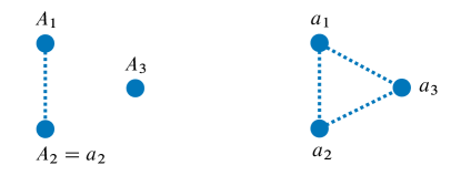
Figure 4: Three mode state defined by $A_{i}$ (left panel) and defined by $a_{i}^{\text{out}}$ (right panel). $A_{1}$ and $A_{2}$ constitute a pure two mode squeezed state and $A_{3}$ has no correlation with them. Expressing the state using the original modes defined by $a_{i}^{\text{out}}$, entanglement of the system is shared by all three modes.

To obtain the wave function of the in-vacuum state involving three modes, we introduce the following canonical quadrature operators

$$\hat{X}_{j}=\frac{\hat{A}_{j}+\hat{A}_{j}{}^{\!\!{\dagger}}}{\sqrt{2}},\quad\hat{P}_{i}=\frac{\hat{A}_{j}-\hat{A}_{j}{}^{\!\!{\dagger}}}{i\sqrt{2}}.$$ (35)

Then the wave function of the in-vacuum sate in $X$-representation is

$$\psi_{0}(X_{1},X_{2},X_{3}) =\bra{X_{1},X_{2},X_{3}}\ket{\psi_{0}}$$

$$=\frac{1}{\cosh r}\sum_{n=0}^{\infty}(-\tanh r)^{n}\bra{X_{1}}\ket{n}_{A_{1}}\bra{X_{2}}\ket{n}_{A_{2}}\bra{X_{3}}\ket{0}_{A_{3}},$$ (36)

where

$$\bra{X_{1,2}}\ket{n}_{A_{1,2}}=\left(2^{n}n!\sqrt{\pi}\right)^{-1/2}H_{n}(X_{1,2})e^{-X_{1,2}^{2}/2},\quad\bra{X_{3}}\ket{0}_{A_{3}}=\left(\sqrt{\pi}\right)^{-1/2}e^{-X_{3}^{2}/2}.$$ (37)

After all, the wave function is

$$\psi_{0}(X_{1},X_{2},X_{3}) =\frac{\pi^{-3/4}}{\cosh r}\,e^{-(X_{1}^{2}+X_{2}^{2}+X_{3}^{2})/2}\sum_{n=0}^{\infty}\frac{(-\tanh r)^{n}}{2^{n}n!}H_{n}(X_{1})H_{n}(X_{2})$$

$$=\pi^{-3/4}\exp\left[-\frac{\cosh 2r}{2}(X_{1}^{2}+X_{2}^{2})+\sinh 2rX_{1}X_{2}-\frac{X_{3}^{2}}{2}\right].$$ (38)

III.3 Wigner function

To analyze structure of the tripartite entanglement of the in-vacuum state, it is convenient to adopt the phase space representation of the wave function. For this purpose, we introduce the Wigner function of the three mode wave function (38)

$$W(\bm{X},\bm{P}): =\frac{1}{(2\pi)^{3}}\int d^{3}\bm{y}\,e^{i\bm{P}\cdot\bm{y}}\,\psi_{0}\left(\bm{X}+\frac{\bm{y}}{2}\right)\psi_{0}^{*}\left(\bm{X}-\frac{\bm{y}}{2}\right)$$

$$=\frac{1}{\pi^{3}}\exp[-\cosh 2r\,(X_{1}^{2}+P_{1}^{2}+X_{2}^{2}+P_{2}^{2})+2\sinh 2r\,(X_{1}X_{2}-P_{1}P_{2})-(X_{3}^{3}+P_{3}^{2})\Bigr{]}.$$ (39)

In terms of the phase space vector $\bm{\xi}=(X_{1},P_{1},X_{2},P_{2},X_{3},P_{3})^{T}$, the Wigner function is expressed as

$$W(\bm{\xi})=\frac{1}{\pi^{3}}\exp\left[-\frac{1}{2}\bm{\xi}^{T}\bm{V}^{-1}\bm{\xi}\right],\qquad\int d^{6}\bm{\xi}W(\bm{\xi})=1,$$ (40)

where $\bm{V}$ is the covariance matrix

$$V_{ij}=\frac{1}{2}\expectationvalue{\hat{\xi}_{i}\hat{\xi}_{j}+\hat{\xi}_{j}\hat{\xi}_{i}}=\int d^{6}\bm{\xi}\,\xi_{i}\xi_{j}W(\bm{\xi}),\quad i,j=1,\cdots 6,$$ (41)

and its components are

$$\bm{V}=\frac{1}{2}\begin{bmatrix}\cosh 2r\bm{I}&-\sinh 2r\bm{Z}&0\\ -\sinh 2r\bm{Z}&\cosh 2r\bm{I}&0\\ 0&0&\bm{I}\end{bmatrix},\quad\bm{I}=\begin{bmatrix}1&0\\ 0&1\end{bmatrix},\quad\bm{Z}=\begin{bmatrix}1&0\\ 0&-1\end{bmatrix}.$$ (42)

The original canonical quadrature operators associated with $\hat{a}_{j}^{\text{out}},\hat{a}_{j}^{\text{out}}{}^{\dagger}$ are

$$\hat{x}_{j}=\frac{\hat{a}_{j}^{\text{out}}+\hat{a}_{j}^{\text{out}}{}^{{\dagger}}}{\sqrt{2}},\quad\hat{p}_{j}=\frac{\hat{a}_{j}^{\text{out}}-\hat{a}_{j}^{\text{out}}{}^{{\dagger}}}{i\sqrt{2}}.$$ (43)

The relation between $\bm{\xi}_{0}=(x_{1},p_{1},x_{2},p_{2},x_{3},p_{3})^{T}$ and $\bm{\xi}=(X_{1},P_{1},X_{2},P_{2},X_{3},P_{3})^{T}$ is obtained from (29):

$$\begin{bmatrix}X_{1}\\ P_{1}\\ X_{2}\\ P_{2}\\ X_{3}\\ P_{3}\end{bmatrix}=\begin{bmatrix}\cos\theta\cos\varphi_{12}&\cos\theta\sin\varphi_{12}&0&0&\sin\theta\cos\varphi_{32}&\sin\theta\sin\varphi_{32}\\ -\cos\theta\sin\varphi_{12}&\cos\theta\cos\varphi_{12}&0&0&-\sin\theta\sin\varphi_{32}&\sin\theta\cos\varphi_{32}\\ 0&0&1&0&0&0\\ 0&0&0&1&0&0\\ \sin\theta\cos\varphi_{3}&-\sin\theta\sin\varphi_{3}&0&0&-\cos\theta\cos\varphi_{1}&\cos\theta\sin\varphi_{1}\\ \sin\theta\sin\varphi_{3}&\sin\theta\cos\varphi_{3}&0&0&-\cos\theta\sin\varphi_{1}&-\cos\theta\cos\varphi_{1}\end{bmatrix}\begin{bmatrix}x_{1}\\ p_{1}\\ x_{2}\\ p_{2}\\ x_{3}\\ p_{3}\end{bmatrix},$$ (44)

where $\varphi_{ij}:=\varphi_{i}-\varphi_{j}$. We denote this relation as $\bm{\xi}=\bm{S}\bm{\xi}_{0}$. As $\bm{S}$ is a symplectic transformation, it satisfies the symplectic condition

$$\bm{S}\bm{\Omega}_{3}\bm{S}^{T}=\bm{\Omega}_{3},\quad\bm{\Omega}_{3}:=\bigoplus_{j=1}^{3}\bm{J},\quad\bm{J}=\begin{bmatrix}0&1\\ -1&0\end{bmatrix}.$$ (45)

The Wigner function $W_{0}$ for the original variables $\bm{\xi}_{0}$ is

$$W_{0}(\bm{\xi}_{0})=W(\bm{S}\bm{\xi}_{0})=\frac{1}{\pi^{3}}\exp\left[-\frac{1}{2}\bm{\xi}_{0}^{T}\bm{S}^{T}\bm{V}^{-1}\bm{S}\bm{\xi}_{0}\right]=\frac{1}{\pi^{3}}\exp\left[-\frac{1}{2}\bm{\xi}_{0}^{T}\bm{V}_{0}^{-1}\bm{\xi}_{0}\right],$$ (46)

where the covariance matrix $\bm{V}_{0}$ is related to $\bm{V}$ as

$$\bm{V}_{0}=\bm{S}^{-1}\bm{V}(\bm{S}^{T})^{-1}=\bm{\Omega}_{3}\bm{S}^{T}\bm{\Omega}_{3}\bm{V}\bm{\Omega}_{3}\bm{S}\bm{\Omega}_{3},$$ (47)

and its components are given by

$$\bm{V}_{0}=\begin{bmatrix}\bm{V}_{1}&\bm{W}_{12}&\bm{W}_{31}\\ \bm{W}_{12}^{T}&\bm{V}_{2}&\bm{W}_{23}\\ \bm{W}_{31}^{T}&\bm{W}_{23}^{T}&\bm{V}_{3}\end{bmatrix}$$ (48)

with $2\times 2$ submatrices

$$\bm{V}_{1}=\left(\frac{1}{2}+\sinh^{2}r\cos^{2}\theta\right)\,\bm{I},\quad\bm{V}_{2}=\frac{\cosh 2r}{2}\,\bm{I},\quad\bm{V}_{3}=\left(\frac{1}{2}+\sinh^{2}r\sin^{2}\theta\right)\,\bm{I},$$ (49)

$$\bm{W}_{12}=-\frac{\sinh 2r\cos\theta}{2}\begin{bmatrix}\cos\varphi_{12}&\sin\varphi_{12}\\ \sin\varphi_{12}&-\cos\varphi_{12}\end{bmatrix},\quad\bm{W}_{23}=-\frac{\sinh 2r\sin\theta}{2}\begin{bmatrix}\cos\varphi_{32}&\sin\varphi_{32}\\ \sin\varphi_{32}&-\cos\varphi_{32}\end{bmatrix},$$

$$\bm{W}_{31}=\frac{\sinh^{2}r\sin 2\theta}{2}\begin{bmatrix}\cos\varphi_{13}&-\sin\varphi_{13}\\ \sin\varphi_{13}&\cos\varphi_{13}\end{bmatrix}.$$ (50)

As the total system is pure, the covariance matrix $\bm{V}_{0}$ satisfies the following purity condition Giedke2014

$$\bm{V}_{0}\bm{\Omega}_{3}\bm{V}_{0}=\frac{1}{4}\,\bm{\Omega}_{3}.$$ (51)

Submatrices $\bm{W}_{12},\bm{W}_{23},\bm{W}_{31}$ can be simultaneously diagonalized using the local rotation with respect to each mode Giedke2014 . As we are interested in entanglement of the state, and it can be quantified in terms of the symplectic eigenvalues and the negativity determined by the symplectic eigenvalues. They are independent of $\varphi_{1}-\varphi_{2},\varphi_{3}-\varphi_{2},\varphi_{1}-\varphi_{3}$ and for the purpose of obtaining negativities of the state defined by the covariance matrix (52) , we can set $\varphi_{1}=\varphi_{2}=\varphi_{3}$ without loss of generality. After all, entanglement structure of the present three mode model can be investigated using the following covariance matrix

$$\bm{V}_{0}=\frac{1}{2}\begin{bmatrix}\left(1+2\sinh^{2}r\cos^{2}\theta\right)\bm{I}&-\sinh 2r\cos\theta\bm{Z}&\sinh^{2}r\sin 2\theta\bm{I}\\ *&\cosh 2r\bm{I}&-\sinh 2r\sin\theta\bm{Z}\\ *&*&\left(1+2\sinh^{2}r\sin^{2}\theta\right)\bm{I}\end{bmatrix}.$$ (52)

Two parameters $r,\theta$ in the covariance matrix are related to the Bogoliubov coefficients as

$$\cosh r=|\alpha_{\bar{u}\bar{u}}|,\quad\tan\theta=\left|\frac{\alpha_{\bar{u}v}}{\alpha_{\bar{u}u}}\right|.$$ (53)

For $\theta=0,\pi$, $\bm{V}_{0}$ reduces to $\bm{V}$ (Eq. (42)). The parameter $\theta$ represents degree of $\bar{u}v$-mixing.

By tracing out modes 23, 31, 12, reduced single mode states are

$$\hat{\rho}_{1}:=\mathrm{Tr}_{2,3}\hat{\rho},\quad\hat{\rho}_{2}:=\mathrm{Tr}_{3,1}\hat{\rho},\quad\hat{\rho}_{3}=\mathrm{Tr}_{1,2}\hat{\rho},$$ (54)

and their covariance matrices are given by $\bm{V}_{1},\bm{V}_{2},\bm{V}_{3}$, respectively. By tracing out modes 3,1,2, reduced bipartite states are

$$\hat{\rho}_{12}:=\mathrm{Tr}_{3}\hat{\rho},\quad\hat{\rho}_{23}:=\mathrm{Tr}_{1}\hat{\rho},\quad\hat{\rho}_{31}:=\mathrm{Tr}_{2}\hat{\rho},$$ (55)

and their covariance matrices are

$$\bm{V}_{12}=\frac{1}{2}\begin{bmatrix}(1+2\sinh^{2}r\cos^{2}\theta)\bm{I}&-\sinh 2r\cos\theta\bm{Z}\\ -\sinh 2r\cos\theta\bm{Z}&\cosh 2r\bm{I}\end{bmatrix},$$ (56)

$$\bm{V}_{23}=\frac{1}{2}\begin{bmatrix}\cosh 2r\bm{I}&-\sinh 2r\sin\theta\bm{Z}\\ -\sinh 2r\sin\theta\bm{Z}&(1+2\sinh^{2}r\sin^{2}\theta)\bm{I}\end{bmatrix},$$ (57)

$$\bm{V}_{31}=\frac{1}{2}\begin{bmatrix}(1+2\sinh^{2}r\sin^{2}\theta)\bm{I}&\sinh^{2}r\sin 2\theta\bm{I}\\ \sinh^{2}r\sin 2\theta\bm{I}&(1+2\sinh^{2}r\cos^{2}\theta)\bm{I}\end{bmatrix}.$$ (58)

III.4 Negativity and tripartite entanglement

In this paper, we adopt the negativity as an entanglement measure. For a Gaussian state with canonical variables $\hat{\bm{\xi}}=(\hat{x}_{1},\hat{p}_{1},\cdots,\hat{x}_{N},\hat{p}_{N})^{T},\langle\hat{\bm{\xi}}\rangle=0$, the commutation relation is

$$[\hat{\xi}_{j},\hat{\xi}_{k}]=i(\Omega_{N})_{jk},\quad\bm{\Omega}_{N}=\bigoplus_{j=1}^{N}\bm{J}.$$ (59)

The Gaussian state is completely characterized by the covariance matrix $V_{jk}=\langle{\hat{\xi}_{j}\hat{\xi}_{k}+\hat{\xi}_{k}\hat{\xi}_{j}}\rangle/2$. For a physical state, the density matrix must be non-negative and the corresponding covariance matrix must satisfy the inequality

$$\bm{V}+\frac{i}{2}\bm{\Omega}_{N}\geq 0,$$ (60)

which is the generalization of the uncertainty relation between two canonically conjugate variables. The separability of the bipartite Gaussian state composed of parties A and B is expressed in terms of the partial transpose operation defined by reversing the sign of one party’s momentum Peres1996 ; Horodecki1997 ; Simon2000 . For the partially transposed covariance matrix $\tilde{\bm{V}}$, the sufficient condition of the separability is given by

$$\tilde{\bm{V}}+\frac{i}{2}\bm{\Omega}_{N}\geq 0.$$ (61)

If this inequality is violated, the bipartite state is entangled. To quantify entanglement, we introduce symplectic eigenvalues $\nu_{i}$ of $\bm{V}$, which are obtained by diagonalizing the covariance matrix with a symplectic transformation. Practically, symplectic eigenvalues can be obtained as positive eigenvalues of the matrix $i\bm{\Omega}_{N}\bm{V}$ Weedbrook2012 . In terms of symplectic eigenvalues, the physical condition (60) is $\nu_{i}\geq 1/2$ and the separability condition is $\tilde{\nu}_{i}\geq 1/2$ where $\tilde{\nu}_{i}$ are symplectic eigenvalues of $\tilde{\bm{V}}$. The entanglement negativity Vidal2002a is given by

$$\mathcal{N}:=\frac{1}{2}\mathrm{max}\left[\left(\prod_{\tilde{\nu}_{i}<1/2}\frac{1}{2\tilde{\nu}_{i}}\right)-1,0\right].$$ (62)

Nonzero value of the negativity implies non-separability of the bipartite state and existence of bipartite entanglement of the system. Related to the negativity, the logarithmic negativity is defined by

$$E_{N}:=\log(2\mathcal{N}+1).$$ (63)

Bipartite entanglement of three mode state is evaluated by specifying three possible bipartitions (Fig. 5):

Figure 5: Possible bipartitions of three mode state. For all three different partitions, bipartite entanglement (negativity) is nonzero in the present model. This implies existence of genuine tripartite entanglement which cannot be reducible to bipartite entanglement between reduced two modes.

Behavior of logarithmic negativities $E_{N}{}_{1:23},E_{N}{}_{2:31},E_{N}{}_{3:12}$ is shown in Fig. 6. For three different partitions of three modes, the logarithmic negativity is nonzero and grows as $r$ increases with $\theta$ fixed. This behavior implies the three mode state has genuine tripartite entanglement which cannot be reducible to bipartite entanglement between two modes. For a fixed value of $r$, the following inequalities hold (right panel of Fig. 6)

$$E_{N}{}_{2:31}\geq E_{N}{}_{1:23},\quad E_{N}{}_{2:31}\geq E_{N}{}_{3:12}.$$ (64)

Magnitude relation between $E_{N}{}_{1:23}$ and $E_{N}{}_{3:12}$ changes depending on values of $\theta$.

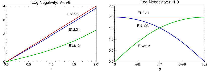
Figure 6: Bipartite entanglement of the three mode state. Amount of entanglement increases as the parameter $r$ increases (left panel). Relative magnitude of $E_{N}{}_{1:23}$ and $E_{N}{}_{3:12}$ changes depending on values of the parameter $\theta$.

By tracing out an one mode of three mode state, entanglement between reduced two modes is also evaluated (Fig 7).

Figure 7: Reduced two modes states are obtained by tracing out one mode. In the present three mode model, $E_{N}{}_{3:1}=0$ and outgoing mode 1 ($u$) and ingoing mode 3 ($v$) are separable as reduced two mode state. However, this does not imply the mode 1 and the mode 3 do not share entanglement.

For reduced two mode states, behavior of the logarithmic negativity is shown in Fig. 8. We have always

$$E_{N}{}_{3:1}=0,$$ (65)

and the mode 1 and the mode 3 are separable as a reduced two mode system. For $\theta=0$, $E_{N}{}_{2:3}=0$ and the modes 1 and 2 forms pure two mode squeezed state and the mode 3 decouples. For $\theta=\pi/2$, $E_{N}{}_{1:2}=0$ and the mode 2 and 3 forms pure two mode squeezed state and the mode 1 decouples.

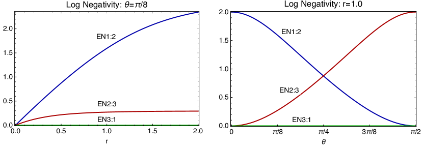
Figure 8: Bipartite entanglement of reduced two modes states. Negativity between the mode 1 and 3 is$E_{N}{}_{3:1}=0$. Relative magnitude of $E_{N}{}_{1:2}$ and $E_{N}{}_{2:3}$ changes depending on values of the parameter $\theta$.

To quantify genuine tripartite entanglement which cannot be reducible to bipartite entanglement between two modes, we examine the residual of entanglement defined by

$$\tau_{1}=E_{1:23}-E_{1:2}-E_{1:3}=E_{1:23}-E_{1:2},$$

$$\tau_{2}=E_{2:31}-E_{1:2}-E_{2:3},$$ (66)

$$\tau_{3}=E_{3:12}-E_{3:1}-E_{3:2}=E_{3:12}-E_{2:3},$$

where $E$ denotes square of the logarithmic negativity. The residual of entanglement quantifies genuine multipartite entanglement and is proved to have positive values for three mode pure Gaussian state Adesso2006b (monogamy relation of entanglement). If the residual is zero, entanglement in three mode state can be represented as summation of entanglement of the reduced two modes state and there is no genuine multipartite entanglement. The tripartite entanglement of the system is also quantified by a single quantity

$$\tau=\mathrm{min}(\tau_{1},\tau_{2},\tau_{3}).$$ (67)

Dependence of $\theta$ of the residual entanglement is shown in Fig. 9.

Figure 9: Residual of entanglement $\tau_{1},\tau_{2},\tau_{3}$ (left panel) and $\tau$ (right panel). Genuine tripartite entanglement exists for $\theta\neq 0,\pi/2$. For $\theta=0,\pi/2$, one mode decouples from other two modes and residual entanglement becomes zero.

For $\theta=0$, the logarithmic negativity is $E_{N}{}_{3:12}=E_{N}{}_{2:3}=0,E_{N}{}_{1:23}=E_{N}{}_{2:31}=E_{N}{}_{1:2}\neq 0$ and $\tau_{1,2,3}=0$. The modes 1,2 constitute a pure entangled state and the mode 3 decouples. Standard scenario of the Hawking radiation corresponds to $\theta=0$ because the mode 3 (left moving $v$ mode) decouples and the mode 2 ($\bar{u}$ mode) becomes the entanglement partner of the mode 1 (the Hawking particle $u$). For $\theta\neq 0,\pi/2$, entanglement of three mode states is shared by all three modes and there is genuine tripartite entanglement.

IV Entanglement of Hawking radiation in dispersive model

So far we obtained the structure of the in-vacuum state defined by three mode Bogoliubov transformation (19) without specifying behavior of coefficients. By obtaining wave modes in dispersive media numerically, it is possible to examine tripartite entanglement of the Hawking radiation.

IV.1 Numerical method

We solve the wave equation (3) to obtain the Bogoliubov coefficients. For this purpose, we consider three different boundary conditions for the wave equation (Fig. 10). Corresponding to the in-state, ingoing modes ($u_{2}$, $\bar{u}$, $v$) are assumed. Three different out-states are possible by choosing different boundary conditions at $x=-\infty$.

Figure 10: Three different combinations of modes to determine the Bogoliubov coefficients. The dotted line represents the sonic horizon.

The mode $\psi_{A}$ is defined by imposing a boundary condition that all wave modes decay at $x\rightarrow-\infty$. This combination of modes corresponds to $\varphi_{u}^{\text{out}}$ in (26). The mode $\psi_{B}$ is defined by imposing a boundary condition that only $\bar{u}$ mode exists at $x\rightarrow-\infty$ and is represented by a linear combination of $\varphi_{\bar{u}}^{\text{out}}$ and $\varphi_{v}^{\text{out}}$: $\psi_{B}\propto(\varphi_{\bar{u}}^{\text{out}})^{*}+c_{1}\varphi_{u}^{\text{out}}$. The mode $\psi_{C}$ is defined by imposing a boundary condition that only $v$ modes exists at $x\rightarrow-\infty$ and is represented by a linear combination of $\varphi_{v}^{\text{out}}$ and $\varphi_{u}^{\text{out}}$: $\psi_{C}\propto\varphi_{v}^{\text{out}}+c_{2}\varphi_{u}^{\text{out}}$. The coefficients $c_{1},c_{2}$ are determined by required boundary conditions. Taking into account of the definition of the Bogoliubov coefficients (26), behaviors of these modes at $x=\pm\infty$ are

$$\psi_{A}\propto\varphi_{u}^{\text{out}}$$

$$\sim\begin{cases}0\quad&(x\rightarrow-\infty)\\ \varphi_{u_{1}}+\alpha_{uu}\varphi_{u_{2}}+\alpha_{\bar{u}u}\varphi_{\bar{u}}^{*}+\alpha_{vu}\varphi_{v},\quad&(x\rightarrow+\infty)\end{cases}$$ (68)

$$\psi_{B}\propto(\varphi_{\bar{u}}^{\text{out}})^{*}+c_{1}\varphi_{u}^{\text{out}}$$

$$\sim\begin{cases}\varphi_{\bar{u}}^{*}\quad&(x\rightarrow-\infty)\\ (\alpha_{u\bar{u}}+c_{1}\alpha_{uu})\varphi_{u_{2}}+(\alpha_{\bar{u}\bar{u}}+c_{1}\alpha_{\bar{u}u})\varphi_{\bar{u}}^{*}+(\alpha_{v\bar{u}}+c_{1}\alpha_{vu})\varphi_{v}+c_{1}\varphi_{u_{1}},\quad&(x\rightarrow+\infty)\end{cases}$$ (69)

$$\psi_{C}\propto\varphi_{v}^{\text{out}}+c_{2}\varphi_{u}^{\text{out}}$$

$$\sim\begin{cases}\varphi_{v}\quad&(x\rightarrow-\infty)\\ (\alpha_{uv}+c_{2}\alpha_{uu})\varphi_{u_{2}}+(\alpha_{\bar{u}v}+c_{2}\alpha_{\bar{u}u})\varphi_{\bar{u}}^{*}+(\alpha_{vv}+c_{2}\alpha_{vu})\varphi_{v}+c_{2}\varphi_{u_{1}}.\quad&(x\rightarrow+\infty)\end{cases}$$ (70)

Asymptotic behavior of these modes at $x\rightarrow+\infty$ can be represented by the Fourier expansion

$$\psi_{A,B,C}\sim\sum_{m}d_{A,B,C}^{(m)}\,\varphi_{m},\quad m=u_{1},u_{2},\bar{u},v,$$ (71)

where $\varphi_{m}\propto e^{ik_{m}(\omega)x}$ are plane waves at the asymptotic region corresponding to each mode. It is possible to obtain the Bogoliubov coefficients from Fourier coefficients $d_{A,B,C}^{(m)}$ of these modes. We integrate the wave equation (3) from the inner boundary of numerical region (corresponds to $x=-\infty$) with specified boundary conditions for $\psi_{A,B,C}$ to the outer numerical boundary (corresponds to $x=+\infty$) across the sonic horizon $x=0$, and read off coefficients $d^{(m)}_{A,B,C}$.

We adopted the 4th order Runge-Kutta method to solve the wave equation. For numerical calculation, we prepare computation region $-20\leq x\leq 250$ with discretization $\Delta x=0.001$. The parameters of the velocity profile $V(x)$ are $D=0.7,\kappa=7$. The corresponding Hawking temperature is $T_{H}=\kappa/(2\pi)=1.11$. The cutoff parameters in the dispersion are chosen as $k_{0}=2,15$, which correspond to $\omega_{\text{cutoff}}=0.6,4.5$. Thus these two cutoff parameter correspond to $\omega_{\text{cutoff}}<T_{H}$ for $k_{0}=2$ and $\omega_{\text{cutoff}}>T_{H}$ for $k_{0}=15$. Calculated range of the frequency is $0<\omega<\omega_{\text{cutoff}}$ with $\Delta\omega=0.0001$. Figure 11 shows behaviors of $\psi_{A,B,C}$ with $k_{0}=15,\omega=0.1$; they reflect different boundary conditions at $x=-20$ which is the inner boundary of our numerical integration.

Figure 11: Three mode functions to obtain the Bogoliubov coefficients (figure shows $k_{0}=15,\omega=0.1$ case). Blue lines and red lines correspond to the real part and the imaginary part of each wave function, respectively. The mode function $\psi_{A}$ does not show oscillatory behavior in $x<0$ region. The mode functions $\psi_{B}$ and $\psi_{C}$ show oscillation in $x<0$ which correspond to propagating $\bar{u}$ mode and $v$ mode, respectively.

IV.2 Result

From the Bogoliubov transformation (19), the number of outgoing Hawking particles (mode $u$) for the in-vacuum state $\ket{\psi_{0}}$ is

$$N_{u}(\omega)=\bra{\psi_{0}}\hat{a}_{u}^{\text{out}}{}^{{\dagger}}\hat{a}_{u}^{\text{out}}\ket{\psi_{0}}=|\alpha_{\bar{u}u}|^{2}\,\delta(0)$$ (72)

where the divergent factor $\delta(0)$ accounts for an infinite spatial volume. The mean number density of particles is $n_{u}(\omega)=|\alpha_{\bar{u}u}|^{2}$. We compare numerically obtained $|\alpha_{\bar{u}u}|^{2}$ with the following spectrum with $\omega$ dependent temperature $T(\omega)$ Macher2009 ; Macher2009b :

$$n_{u}(\omega)=\frac{1}{e^{\omega/T(\omega)}-1}.$$ (73)

Figure 12 shows the spectrum of particle number density obtained by our numerical calculation. For $\omega\ll\omega_{\text{cutoff}}$, the spectrum agrees well with the thermal one but its temperature differs from the Hawking temperature $T_{H}$ (see Fig. 13). For small cutoff frequency $\omega_{\text{cutoff}}<T_{H}$, the temperature is proportional to $\omega_{\text{cutoff}}$. As the cutoff frequency becomes larger and satisfies $T_{H}<\omega_{\text{cutoff}}$, the thermal temperature approaches $T_{H}$ Macher2009b . The value of temperature is related to the location where the mode conversion occurs. For large cutoff $T_{H}<\omega_{\text{cutoff}}$, the left moving wave $u_{2}$ is reflected in the vicinity of the sonic horizon and the thermal temperature is determined by the “surface gravity” of the sonic horizon. On the other hand for small cutoff frequency $\omega_{\text{cutoff}}<T_{H}$, the mode conversion occurs at the location (9) depart from the sonic horizon and the thermal temperature is lowered.

Figure 12: Left panel: the spectrum of created particle number density $n_{u}(\omega)=|\alpha_{\bar{u}u}|^{2}$ for $k_{0}=2,15$. The cutoff frequency is $\omega_{\text{cutoff}}=0.6,4.5$. Right panel shows effective temperature $T(\omega)$ defined by (73). For $\omega\ll\omega_{\text{cutoff}}$, the spectrum is well fitted with thermal ones but its temperature differs from $T_{H}$ for $k_{0}=2$. As the cutoff frequency becomes larger, the temperature approaches $T_{H}$.

Figure 13: The cutoff parameter dependence of the thermal temperature at $\omega=0.001$. Open circles correspond to cutoff wave numbers $k_{0}=1,2,4,10,15$. For $\omega_{\text{cutoff}}<T_{H}~{}(k_{0}<3.71)$, the temperature is proportional to $\omega_{\text{cutoff}}$. For $\omega_{c}>T_{H}~{}(k_{0}>3.71)$, the temperature asymptotically approaches $T_{H}$ as the cutoff frequency increases.

The entanglement structure of the state with the covariance matrix (52) is encoded in behavior of parameters $r(\omega),\theta(\omega)$, which are determined by the Bogoliubov coefficients $\alpha_{\bar{u}u},\alpha_{\bar{u}\bar{u}},\alpha_{\bar{u}v}$. Figure 14 shows $\omega$-dependence of these parameters obtained from our numerical calculation. As the number density of the Hawking particles is $|\alpha_{\bar{u}u}|^{2}=\cos^{2}\theta\sinh^{2}r$, emission of radiation is monotonically decreases as $\omega$ increases.

Figure 14: Frequency dependence of parameters $r,\theta$ for $k_{0}=2,15$. Around $\omega\sim\omega_{\text{cutoff}}$, the squeezing parameter $r$ becomes smaller than one and emission of the Hawking radiation is shut down.

Figure 15 shows behavior of the logarithmic negativity for $k_{0}=15$ ($T_{H}<\omega_{\text{cutoff}}$ case). Left panel shows bipartite entanglement for three different bipartitions. For $\omega\ll\omega_{\text{cutoff}}$, $E_{N}{}_{3:12}\ll E_{N}{}_{2:31}\approx E_{N}{}_{1:23}$ and entanglement of the system is mainly shared by the mode 1 ($u$) and 2 ($\bar{u}$). For $\omega\sim\omega_{\text{cutoff}}$, $E_{N}{}_{1:23}\approx E_{N}{}_{2:31}\approx E_{N}{}_{3:12}$ and entanglement is equally shared by all three modes. Right panel shows bipartite entanglement for reduced two mode states. An equality $E_{N}{}_{3:1}=0$ always holds. We can confirm that the mode 1 $(u)$ and 2 $(\bar{u})$ constitutes a entangled pair for $\omega\ll\omega_{\text{cutoff}}$ because entanglement of the system is mainly shared by the mode 1,2 $(u,\bar{u})$ and the mode 3 $(v)$ decouples. Figure 16 shows behavior of the logarithmic negativity for $k_{0}=2$ ($\omega_{\text{cutoff}}<T_{H}$ case). Although values of entanglement at $\omega\sim 0$ and $\omega\sim\omega_{\text{cutoff}}$ are ten times larger compared to $k_{0}=15$ case, qualitative dependence of $\omega$ is the same as $k_{0}=15$ case.

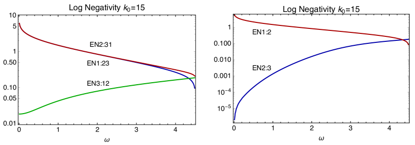
Figure 15: Logarithmic negativity for $k_{0}=15$ ($\omega_{\text{cutoff}}=4.5$). Left panel: logarithmic negativity of the three mode state. Right panel: logarithmic negativity of reduced two mode states. $E_{N}{}_{3:1}=0$ holds.

Figure 16: Log negativity for $k_{0}=2$ ($\omega_{\text{cutoff}}=0.6$). Left panel: logarithmic negativity of three mode state. Right panel: logarithmic negativity of reduced two mode state. $E_{N}{}_{3:1}=0$ holds.

Figure 17 shows behavior of the residual of entanglement. For $\omega<\omega_{\text{cutoff}}$, the genuine tripartite entanglement persists. However, as $\tau_{1,2,3}\ll E_{N3:12}$ and $E_{N}{}_{2:31}\approx E_{N}{}_{1:23}$, $E_{N}{}_{2:3}<E_{N}{}_{1:2}$, the entanglement of the system is mainly shared by the modes $u$ and $\bar{u}$. Thus we can conclude that $\bar{u}$ mode is approximately the partner mode of the Hawking particle $u$. For $\omega\sim\omega_{\text{cutoff}}$, the residual of entanglement approaches nonzero small value and the entanglement of the system is approximately equally shared by pairs of the modes $v,\bar{u}$ and $u,\bar{u}$. Thus the tripartite entanglement is reducible to the bipartite entanglement between two modes (Fig. 18).

Figure 17: Behavior of the residual entanglement (left panel: $\omega_{\text{cutoff}}=4.5$, right panel: $\omega_{\text{cutoff}}=0.6$). For $\omega<\omega_{\text{cutoff}}$, the residual $\tau_{1,2,3}$ has nonzero value. However, as $\tau_{1,2,3}\ll E_{N}{}_{3:12}$, the tripartite entanglement of the system can be approximately reducible to the bipartite entanglement between mode 1 $(u)$ and 2 $(\bar{u})$. For $\omega\sim\omega_{\text{cutoff}}$, $\tau_{1,2,3}$ approach to nonzero small values and the tripartite entanglement of the system can be approximately reducible to the bipartite entanglement between mode 1, 2 $(u,\bar{u})$ and 2,3 $(\bar{u},v)$.

Figure 18: Schematic structure of the tripartite entanglement in dispersive model. For low frequency $\omega\ll\omega_{\text{cutoff}}$, the mode 1 ($u$) and 2 ($\bar{u}$) constitute an entangled pair because genuine tripartite entanglement is small. For $\omega\sim\omega_{\text{cutoff}}$, genuine tripartite approaches zero and entanglement of the system is equally shared by the modes 1,2 ($u,\bar{u}$) and the modes 2,3 ($\bar{u},v$).

The spectrum of the Hawking radiation around $\omega\ll\omega_{\text{cutoff}}$ well agrees with the thermal one with a temperate given by $T\sim T_{H}$ for $\omega_{\text{cutoff}}>T_{H}$ and $T\propto\omega_{\text{cutoff}}$ for $\omega_{\text{cutoff}}<T_{H}$. From the viewpoint of entanglement, although genuine tripartite entanglement exists around $\omega<\omega_{\text{cutoff}}$, its amount is smaller than the bipartite entanglement between the mode 1 $(u)$ and 2 $(\bar{u})$. Thus the mode 1 $(u)$ and 2 ($\bar{u}$) constitute entangled pair and the mode 3 $(v)$ decouples. Thus the expected spectrum of emitted radiation (mode $u$) coincides with the thermal one because reduced state of the mode $u$ is a state of maximal entropy. For frequency around $\omega_{\text{cutoff}}$, entanglement of the system is equally shared by the modes $u,\bar{u}$ and the modes $\bar{u},v$. Hence the reduced state of the mode $u$ does not show the thermal feature.

V Conclusion

We examined effect of multipartite entanglement on the Hawking radiation in the dispersive model and found that the tripartite entanglement persists in the whole frequency range up to $\omega_{\text{cutoff}}$. The origin of this multipartite entanglement is mixing of the left moving $v$ mode and remaining $u,\bar{u}$ modes. Usually, this mixing is recognized as the gray-body factor due to back scattering of waves. In the dispersive model investigated in this paper, the origin of the gray-body factor is spatially varying background flow velocity Anderson2014 ; Anderson2015 ; Fabbri2016 . Thus even for low frequency region where the fluid is nearly dispersionless, nonzero values of the tripartite entanglement is expected as confirmed by our numerical calculation. The effect of this mixing and relation to the tripartite entanglement has not been considered in previous investigations. For low frequency region, the mixing between the $v$ mode and $u,\bar{u}$ modes are small compared to that between $u$ and $\bar{u}$, and resulting spectrum of the Hawking radiation coincides with the thermal one but its temperature depends on the cutoff scale. Emergence of the thermal feature corresponds to the structure of entangled pair $u,\bar{u}$ and decoupling of $v$. Around the cutoff frequency, the thermal feature of the Hawking radiation is lost; entanglement of the system is equally shared by pairs of $v$-$\bar{u}$ and $u$-$\bar{u}$. In this region, the in-vacuum state is a three mode entangled state and this entanglement does not reduce only to that between the Hawking mode $u$ and its partner $\bar{u}$.

If we consider the Hawking radiation for gravitational black holes, $u(\bar{u})$-$v$ mixing naturally occurs due to the gray-body factor which comes from curvature scattering effect. Thus the tripartite entanglement of the Hawking radiation is also expected but the behavior in low frequency region will depend on type of black holes and type of quantum fields. For the massless mininally coupled scalar field, the gray-body factor for the $s$-wave in low frequency limit is zero for the Schwarzschild black hole and nonzero for the Schwarzschild-de Sitter black hole, but the behavior is different for the nonminimally coupled scalar field Kanti2005 ; Anderson2015 . Thus behavior of the tripartite entanglement of the Hawking radiation also depends on the spacetime structures and type of quantum fields.

As remaining issues not investigated in this paper, the first one is effect of different type of dispersion (e.g. superluminal type) on entanglement. In this paper, we have derived the exact form of the in-vacuum state involving three modes without specifying the dispersion relation. As the difference of dispersion is encoded in frequency dependence of the Bogoliubov coefficients, it is simple task to apply our formula to other dispersive models to investigate entanglement structure. The second one is effect of nonvacuum in-state. If we assume the thermal state as the in-state, which corresponds to classical noise from the external environment, the quantum correlation is reduced and the structure of the multipartite entanglement will be affected. The third one is the dependence of flow profile $D,\kappa$ on entanglement. The shape of background flow profile may strongly affects the structure of multipartite entanglement and it is interesting problem to examine difference of velocity profile on structure of entanglement sharing of the Hawking radiation. These problems are left for our future research.

After uploading our paper to arXiv, we noticed the preprint Isoard2021 . In this paper, the authors also investigate the tripartite entanglement of the Hawking radiation for the superluminal dispersion and discuss the best experimental configuration for observing entanglement in the BEC system.

References

• (1) S. W. Hawking, “Black hole explosions?”, Nature 248, (1974) 30–31.
• (2) S. W. Hawking, “Particle creation by black holes”, Commun. Math. Phys. 43, (1975) 199–220.
• (3) W. Unruh, “Sonic analogue of black holes and the effects of high frequencies on black hole evaporation”, Phys. Rev. D 51, (1995) 2827–2838.
• (4) R. Brout, S. Massar, R. Parentani, and P. Spindel, “Hawking radiation without trans-Planckian frequencies”, Phys. Rev. D 52, (1995) 4559–4568.
• (5) S. Corley and T. Jacobson, “Hawking spectrum and high frequency dispersion.”, Phys. Rev. D 54, (1996) 1568–1586.
• (6) Y. Himemoto and T. Tanaka, “Generalization of the model of Hawking radiation with modified high frequency dispersion relation”, Phys. Rev. D 61, (2000) 064004.
• (7) T. Jacobson, “Introduction to Quantum Fields in Curved Spacetime and the Hawking Effect”, in “Lect. Quantum Gravity”, No. January, 39–89 (Springer-Verlag, New York, 2003).
• (8) W. Unruh and R. Schützhold, “Universality of the Hawking effect”, Phys. Rev. D 71, (2005) 024028.
• (9) J. Macher and R. Parentani, “Black-hole radiation in Bose-Einstein condensates”, Phys. Rev. A 80, (2009) 043601.
• (10) J. Macher and R. Parentani, “Black/white hole radiation from dispersive theories”, Phys. Rev. D 79, (2009) 124008.
• (11) S. J. Robertson, “The theory of Hawking radiation in laboratory analogues”, J. Phys. B 45, (2012) 163001.
• (12) U. Leonhardt and S. Robertson, “Analytical theory of Hawking radiation in dispersive media”, New J. Phys. 14, (2012) 053003.
• (13) A. Coutant, R. Parentani, and S. Finazzi, “Black hole radiation with short distance dispersion, an analytical S-matrix approach”, Phys. Rev. D 85, (2012) 024021.
• (14) M. Hotta, R. Schützhold, and W. G. Unruh, “Partner particles for moving mirror radiation and black hole evaporation”, Phys. Rev. D 91, (2015) 1–12.
• (15) X. Busch and R. Parentani, “Quantum entanglement in analogue Hawking radiation: When is the final state nonseparable?”, Phys. Rev. D 89, (2014) 105024.
• (16) A. Peres, “Separability Criterion for Density Matrices”, Phys. Rev. Lett. 77, (1996) 1413–1415.
• (17) P. Horodecki, “Separability criterion and inseparable mixed states with positive partial transposition”, Phys. Lett. A 232, (1997) 333–339.
• (18) R. Simon, “Peres-Horodecki Separability Criterion for Continuous Variable Systems”, Phys. Rev. Lett. 84, (2000) 2726–2729.
• (19) P. R. Anderson, R. Balbinot, A. Fabbri, and R. Parentani, “Gray-body factor and infrared divergences in 1D BEC acoustic black holes”, Phys. Rev. D 90, (2014) 104044.
• (20) P. R. Anderson, A. Fabbri, and R. Balbinot, “Low frequency gray-body factors and infrared divergences: Rigorous results”, Phys. Rev. D 91, (2015) 064061.
• (21) A. Fabbri, R. Balbinot, and P. R. Anderson, “Scattering coefficients and gray-body factor for 1D BEC acoustic black holes: Exact results”, Phys. Rev. D 93, (2016) 1–6.
• (22) A. Recati, N. Pavloff, and I. Carusotto, “Bogoliubov theory of acoustic Hawking radiation in Bose-Einstein condensates”, Phys. Rev. A 80, (2009) 1–10.
• (23) G. Giedke and B. Kraus, “Gaussian local unitary equivalence of n -mode Gaussian states and Gaussian transformations by local operations with classical communication”, Phys. Rev. A 89, (2014) 012335.
• (24) C. Weedbrook, S. Pirandola, R. García-Patrón, N. J. Cerf, T. C. Ralph, J. H. Shapiro, and S. Lloyd, “Gaussian quantum information”, Rev. Mod. Phys. 84, (2012) 621–669.
• (25) G. Vidal and R. Werner, “Computable measure of entanglement”, Phys. Rev. A 65, (2002) 032314.
• (26) G. Adesso and F. Illuminati, “Continuous variable tangle, monogamy inequality, and entanglement sharing in Gaussian states of continuous variable systems”, New J. Phys. 8, (2006) 15–15.
• (27) P. Kanti, J. Grain, and A. Barrau, “Bulk and brane decay of a $(4+n)$-dimensional Schwarzschild-de Sitter black hole: Scalar radiation”, Phys. Rev. D 71, (2005) 1–18.
• (28) M. Isoard, N. Milazzo, N. Pavloff, and O. Giraud, “Bipartite and tripartite entanglement in a Bose-Einstein acoustic black hole”, arXiv: 2102.06175.