Abstract

This paper presents a fast first-order method for solving the quasi-static contact problem with the Coulomb friction. It is known that this problem can be formulated as a second-order cone linear complementarity problem, for which regularized or semi-smooth Newton methods are widely used. As an alternative approach, this paper develops a method based on an accelerated primal-dual algorithm. The proposed method is easy to implement, as most of computation consists of additions and multiplications of vectors and matrices. Numerical experiments demonstrate that this method outperforms a regularized and smoothed Newton method for second-order cone complementarity problems.

Keywords

Optimization; complementarity problem; second-order cone; primal-dual algorithm; contact mechanics; Coulomb friction.

1 Introduction

Frictional contact is ubiquitous in engineering applications, and its computational aspect has been studied extensively [44, 2, 9, 32]. Consider two bodies in the three-dimensional space. When the signed distance between their boundaries, called the gap, is positive, there exists no interaction in terms of forces. Alternatively, if the gap is equal to zero, then the contact pressure force, called the normal reaction, can be present at interface. This relation, which evidently possesses disjunction nature, is called the normal contact law. When the gap is equal to zero, the tangential reaction can also be present due to friction. The most fundamental model of friction is Coulomb’s law. The relative tangential velocity of the two bodies at contact interface is whether equal to zero (said to be stick) or not (said to be slip or slide). The slip can occur when the magnitude of the tangential reaction is equal to a threshold value (which is proportional to the magnitude of the normal reaction), where the tangential reaction is in parallel with the relative tangential velocity in the opposite direction. In contrast, only stick is admissible when the magnitude of the tangential reaction is smaller than the threshold. Thus, the tangential contact law also possesses disjunction nature.

The disjunction nature in frictional contact can be treated within the framework of complementarity problem. To date, diverse formulations, as well as diverse numerical methods, have been proposed; see, e.g., Acary and Brogliato [2] and Wriggers [44]. This reflects the fact that, as Acary et al. [1] concluded through comprehensive numerical experiments, “there is no universal solver” for the frictional contact problem. Indeed, to the best of the author’s knowledge, there is no algorithm that has guarantee of convergence for the three-dimensional quasi-static incremental contact problem with the Coulomb friction.

In this paper, we address the three-dimensional quasi-static incremental problem of elastic bodies subjected to the unilateral contact with the Coulomb friction, under the assumption of small deformation and linear elasticity. For solving this problem, this paper presents an algorithm based on the primal-dual algorithm (a.k.a. the primal-dual hybrid gradient algorithm) [11, 13, 25, 35]. The primal-dual algorithm has received considerable attention in applications to large-scale optimization problems arising in image processing [11, 12, 8, 19, 14].

If we approximate the friction cone (see (8) in section 2.2 for definition of the friction cone) as a polyhedral cone, the problem considered in this paper is reduced to a linear complementarity problem [33]. In contrast, without use of this approximation, the problem is formulated as a nonlinear complementarity problem. Regularized or semi-smooth Newton methods are mainly used to solve such formulations [4, 16, 17, 41, 6]. Kanno et al. [31] showed that the problem can be recast as a second-order cone linear complementarity problem. To this formulation, various methods developed in the field of mathematical optimization may be applicable (although existing methods do not have a proof of convergence for this formulation, due to the lack of monotonicity; see the formulation in Kanno et al. [31, section 4]). See Yoshise [45] and Chen and Pan [15] for survey on the second-order cone complementarity problem and its numerical solutions. For example, a regularized smoothing Newton method proposed by Hayashi et al. [24] was adopted in Kanno et al. [31].

Recently, accelerated gradient methods (a.k.a. optimal first-order methods) have been successfully developed for solving problems, especially large-scale ones, in applied and computational mechanics. Namely, accelerated proximal gradient methods have been proposed for solving the incremental problems in elastoplasticity with various yield criteria [27, 28, 42, 43], as well as the bi-modulus elasticity problem [30]. It is worth noting that the problems dealt with in the literature above are formulated as convex optimization problems. Specifically, the problem in [27] can be recast as a quadratic programming (QP) problem, the one in [42] can be recast as a second-order cone programming (SOCP) problem, and the ones in [43, 30] can be recast as semidefinite programming (SDP) problems. The numerical experiments demonstrate that these accelerated proximal gradient methods outperform standard solvers implementing primal-dual interior-point methods for QP, SOCP, and SDP. As other types of accelerated gradient methods in mechanics, the reader may refer to an accelerated Uzawa method for the frictionless contact problem [29] and an accelerated steepest descent method for the elasticity problem of trusses with material nonlinearity [21].

In the field of computer graphics, Mazhar et al. [38] proposed an accelerated projected gradient method to (approximately) solve a problem stemming from time-discretization of a rigid multi-body dynamical system involving frictional contact. Through numerical experiments, Melanz et al. [39] concluded that this method is most efficient compared with conventional first-order methods (the projected Jacobi method and the projected Gauss–Seidel method) in this research area and second-order optimization methods (primal-dual interior-point methods). It should be clear that the method of Mazhar et al. [38] does not solve the problem to be solved in dynamic simulation, but is a method to solve a modified problem which is easier than the original one. More concretely, the original problem is a nonlinear complementarity problem that does not correspond to the optimality condition of an optimization problem, while Mazhar et al. [38] solves a convex optimization problem that is obtained by adding modification to the original problem. Such artificial modification certainly alters physical phenomena, and causes artifacts in simulation results as illustrated in Mazhar et al. [38, section 2.3]. It is worth noting that there exists some numerical methods for solving the original problem; e.g., nonsmooth Newton methods [10, 7], a fixed-point method that sequentially solves convex optimization problems [3], etc. These methods are not first-order methods. In contrast, in this paper we consider the quasi-static incremental problem of elastic bodies, and attempt to solve the problem itself, i.e., without adding any modification, via an accelerated first-order method.

The paper is organized as follows. Section 2 summarizes the frictional contact problem considered in this paper. As a main contribution, section 3 presents an algorithm for solving this problem, based on an accelerated primal-dual algorithm. Section 4 performs numerical experiments. Section 5 presents some conclusions.

In our notation, ^⊤ denotes the transpose of a vector or a matrix. For $\boldsymbol{x}\in\mathbb{R}^{n}$, we use $\|\boldsymbol{x}\|$ to denote its Euclidean norm, i.e., $\|\boldsymbol{x}\|=\sqrt{\boldsymbol{x}^{\top}\boldsymbol{x}}$. For $\boldsymbol{x}$, $\boldsymbol{y}\in\mathbb{R}^{n}$, we write $\boldsymbol{x}\perp\boldsymbol{y}$ if $\boldsymbol{x}^{\top}\boldsymbol{y}=0$. We use $\langle\boldsymbol{x},\boldsymbol{y}\rangle$ to denote $\boldsymbol{x}^{\top}\boldsymbol{y}$. For a closed convex function $f:\mathbb{R}^{n}\to\mathbb{R}\cup\{+\infty\}$, its proximal mapping is defined by

$$\mathop{\boldsymbol{\mathsf{prox}}}\nolimits_{f}(\boldsymbol{x})=\operatornamewithlimits{\mathrm{arg\,min}}_{\boldsymbol{z}\in\mathbb{R}^{n}}\Bigl{\{}f(\boldsymbol{z})+\frac{1}{2}\|\boldsymbol{z}-\boldsymbol{x}\|^{2}\Bigr{\}}.$$ (1)

For $S\subseteq\mathbb{R}^{n}$, we use $\delta_{S}:\mathbb{R}^{n}\to\mathbb{R}\cup\{+\infty\}$ to denote its indicator function, i.e.,

$$\delta_{S}(\boldsymbol{x})=\begin{dcases*}0&if $\boldsymbol{x}\in S$,\\ +\infty&otherwise.\end{dcases*}$$

We use $\Pi_{S}(\boldsymbol{x})\in\mathbb{R}^{n}$ to denote the projection of $\boldsymbol{x}\in\mathbb{R}^{n}$ onto $S$, i.e.,

$$\Pi_{S}(\boldsymbol{x})=\operatornamewithlimits{\mathrm{arg\,min}}_{\boldsymbol{z}\in S}\{\|\boldsymbol{z}-\boldsymbol{x}\|\}.$$

For a nonempty convex cone $C\subseteq\mathbb{R}^{n}$, define the dual cone by

$$C^{*}=\{\boldsymbol{s}\in\mathbb{R}^{n}\mid\langle\boldsymbol{s},\boldsymbol{x}\rangle\geq 0\ (\forall\boldsymbol{x}\in C)\}.$$

We readily see that

$$\inf_{\boldsymbol{x}\in\mathbb{R}^{n}}\{\langle\boldsymbol{s},\boldsymbol{x}\rangle+\delta_{C}(\boldsymbol{x})\}=-\delta_{C^{*}}(\boldsymbol{s})$$ (2)

holds.

2 Fundamentals: Quasi-static incremental problem

This section summarizes the quasi-static incremental analysis of an elastic solid, with the Coulomb friction for the unilateral contact. For fundamentals of contact mechanics, see, e.g., Duvaut and Lions [18] and Wriggers [44].

2.1 Contact kinematics

Consider an elastic body in the three-dimensional space. The body is discretized according to the conventional finite element method. Let $d$ denote the number of degrees of freedom of the nodal displacements. We use $\boldsymbol{u}\in\mathbb{R}^{d}$ to denote the nodal displacement vector.

To investigate the time evolution in the specified time interval $[0,T]$, suppose that the time interval is subdivided into finitely many intervals. In the quasi-static analysis, we assume that the inertia term in the equation of motion is negligible. This assumption is applicable if the external force applied to the elastic body changes sufficiently slowly. For a specific time subinterval, denoted by $[t^{l},t^{l+1}]$, let $\boldsymbol{u}^{l}$ and $\boldsymbol{u}^{l+1}$ denote the nodal displacements at time $t^{l}$ and $t^{l+1}$, respectively. The incremental problem solved for time $t^{l+1}$ is to find $\boldsymbol{u}^{l+1}$, or, equivalently, to find the incremental displacement [34]

$$\Delta\boldsymbol{u}=\boldsymbol{u}^{l+1}-\boldsymbol{u}^{l}.$$

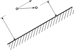
Figure 1: Contact candidate node and obstacle.

For simplicity, we restrict ourselves to the case that the boundary of an elastic body can possibly touch the surface of a fixed rigid obstacle; extension of the proposed method to the case that two elastic bodies can touch each other is straightforward. We assume that a set of contact candidate nodes (i.e., nodes that can possibly contact with the obstacle at time $t=t^{l+1}$) is specified a priori. Figure 1 depicts one of contact candidate nodes. It should be clear that we do not know in advance whether each contact candidate node contacts with the obstacle or not at $t=t^{l+1}$ (because $\Delta\boldsymbol{u}$ is unknown).

Let $c$ denote the number of contact candidate nodes. For contact candidate node $j$ $(j=1,\dots,c)$, let $g_{j}$ denote the initial gap (i.e., the distance between node $j$ and the obstacle at time $t=t^{l}$), which is a nonnegative constant; see Figure 1. The gap at time $t=t^{l+1}$, denoted by $\hat{g}_{j}(\Delta\boldsymbol{u})$, is given in the form

$$\hat{g}_{j}(\Delta\boldsymbol{u})=g_{j}-\boldsymbol{t}_{\mathrm{n}j}^{\top}\,\Delta\boldsymbol{u}$$ (3)

with a constant vector $\boldsymbol{t}_{\mathrm{n}j}\in\mathbb{R}^{d}$, because we assume small deformation. The incremental displacement of node $j$ can be decomposed additively into two components, which are normal and tangential to the obstacle surface. The tangential component, denoted by $\Delta\boldsymbol{u}_{\mathrm{t}j}$, is given in the form

$$\Delta\boldsymbol{u}_{\mathrm{t}j}=T_{\mathrm{t}j}^{\top}\,\Delta\boldsymbol{u},$$ (4)

where $T_{\mathrm{t}j}\in\mathbb{R}^{d\times 2}$ is a constant matrix; see Klarbring [34] for more details. For notational simplicity, define $T_{\mathrm{n}}\in\mathbb{R}^{d\times c}$ and $T_{\mathrm{t}}\in\mathbb{R}^{d\times 2c}$ by

$$T_{\mathrm{n}}=\begin{bmatrix}\boldsymbol{t}_{\mathrm{n}1}&\cdots&\boldsymbol{t}_{\mathrm{n}c}\\ \end{bmatrix},\quad T_{\mathrm{t}}=\begin{bmatrix}T_{\mathrm{t}1}&\cdots&T_{\mathrm{t}c}\\ \end{bmatrix}.$$

If the gap $\hat{g}_{j}(\Delta\boldsymbol{u})$ is equal to zero, then the contact reaction force can be present at node $j$. The reaction also has two components, denoted by $r_{\mathrm{n}j}\in\mathbb{R}$ and $\boldsymbol{r}_{\mathrm{t}j}\in\mathbb{R}^{2}$, which are normal and tangential to the obstacle surface, respectively. It is worth noting that $r_{\mathrm{n}j}$ stems from a kinematic constraint that node $j$ cannot penetrate the obstacle, while $\boldsymbol{r}_{\mathrm{t}j}$ is due to friction. For notational convenience, define $\boldsymbol{r}_{j}\in\mathbb{R}^{3}$, $\boldsymbol{r}\in\mathbb{R}^{3c}$, $\boldsymbol{r}_{\mathrm{n}}\in\mathbb{R}^{c}$, and $\boldsymbol{r}_{\mathrm{t}}\in\mathbb{R}^{2c}$ by

$$\boldsymbol{r}_{j}=\begin{bmatrix}r_{\mathrm{n}j}\\ \boldsymbol{r}_{\mathrm{t}j}\\ \end{bmatrix},\quad\boldsymbol{r}=\begin{bmatrix}\boldsymbol{r}_{1}\\ \vdots\\ \boldsymbol{r}_{c}\\ \end{bmatrix},\quad\boldsymbol{r}_{\mathrm{n}}=\begin{bmatrix}r_{\mathrm{n}1}\\ \vdots\\ r_{\mathrm{n}c}\\ \end{bmatrix},\quad\boldsymbol{r}_{\mathrm{t}}=\begin{bmatrix}\boldsymbol{r}_{\mathrm{t}1}\\ \vdots\\ \boldsymbol{r}_{\mathrm{t}c}\\ \end{bmatrix}.$$

2.2 Coulomb’s friction law under unilateral contact

Let $\mu$ denote the coefficient of friction, which is a positive constant. For the incremental problem, the Coulomb friction law for unilateral contact is given by [18, 44]

$${-}\mu r_{\mathrm{n}j}\geq\|\boldsymbol{r}_{\mathrm{t}j}\|,$$ (5a)

$${-}\mu r_{\mathrm{n}j}>\|\boldsymbol{r}_{\mathrm{t}j}\| \quad\Rightarrow\quad\Delta\boldsymbol{u}_{\mathrm{t}j}=\boldsymbol{0},$$ (5b)

$${-}\mu r_{\mathrm{n}j}=\|\boldsymbol{r}_{\mathrm{t}j}\|>0 \quad\Rightarrow\quad\exists\alpha\geq 0:\ \Delta\boldsymbol{u}_{\mathrm{t}j}=-\alpha\boldsymbol{r}_{\mathrm{t}j}.$$ (5c)

Here, (5a) is inclusion of the reaction into the friction cone, which implies $r_{\mathrm{n}j}\leq 0$, i.e., there exists no adhesion. Disjunction of the sticking and slipping states is described in (5b) and (5c).

Besides the non-adhesion condition (i.e., $r_{\mathrm{n}j}\leq 0$), the unilateral contact condition consists of [18, 44]

$$\hat{g}_{j}(\Delta\boldsymbol{u})\geq 0,$$ (6a)

$$\hat{g}_{j}(\Delta\boldsymbol{u})>0 \quad\Rightarrow\quad r_{\mathrm{n}j}=0,$$ (6b)

$$r_{\mathrm{n}j}<0 \quad\Rightarrow\quad\hat{g}_{j}(\Delta\boldsymbol{u})=0.$$ (6c)

Here, (6a) is the non-penetration condition. We say that node $j$ is in the free state and in contact (with nonzero reaction), respectively, if (6b) and (6c) hold.

It is known that (5) and (6) can be rewritten equivalently as [37, 36]

$$\hat{g}_{j}(\Delta\boldsymbol{u})\geq 0,$$ (7a)

$${-}\mu r_{\mathrm{n}j}\geq\|\boldsymbol{r}_{\mathrm{t}j}\|,$$ (7b)

$$\langle\boldsymbol{r}_{\mathrm{t}j},\Delta\boldsymbol{u}_{\mathrm{t}j}\rangle-\langle r_{\mathrm{n}j},\hat{g}_{j}(\boldsymbol{u})+\mu\|\Delta\boldsymbol{u}_{\mathrm{t}j}\|\rangle=0.$$ (7c)

Let $F\subset\mathbb{R}^{3}$ denote the friction cone, i.e.,

$$F=\{(r_{\mathrm{n}},\boldsymbol{r}_{\mathrm{t}})\in\mathbb{R}\times\mathbb{R}^{2}\mid-\mu r_{\mathrm{n}}\geq\|\boldsymbol{r}_{\mathrm{t}}\|\}.$$ (8)

The dual cone of $F$ is

$$F^{*}=\{(v_{\mathrm{n}},\boldsymbol{v}_{\mathrm{t}})\in\mathbb{R}\times\mathbb{R}^{2}\mid-v_{\mathrm{n}}\geq\mu\|\boldsymbol{v}_{\mathrm{t}}\|\}.$$

Since (7a) holds if and only if $-\hat{g}_{j}(\Delta\boldsymbol{u})-\mu\|\Delta\boldsymbol{u}_{\mathrm{t}j}\|\in F^{*}$, we see that (7) can be recast as the following cone complementarity condition [26, section 10.3.4.1]:

$$F^{*}\ni\begin{bmatrix}-\hat{g}_{j}(\Delta\boldsymbol{u})-\mu\|\Delta\boldsymbol{u}_{\mathrm{t}j}\|\\ \Delta\boldsymbol{u}_{\mathrm{t}j}\\ \end{bmatrix}\perp\begin{bmatrix}r_{\mathrm{n}j}\\ \boldsymbol{r}_{\mathrm{t}j}\\ \end{bmatrix}\in F.$$ (9)

2.3 Equilibrium equation

Let $K\in\mathbb{R}^{d\times d}$ denote the stiffness matrix of the elastic body, which is symmetric and positive definite. We use $\boldsymbol{p}^{l}\in\mathbb{R}^{d}$ to denote the nodal external force applied to the elastic body at time $t^{l}$.

At an equilibrium state, the internal force, the external force, and the reaction are balanced. At time $t^{l}$, this balance law, called the equilibrium equation, is given by [34, 44]

$$K\boldsymbol{u}^{l}-\boldsymbol{p}^{l}=T_{\mathrm{n}}\boldsymbol{r}_{\mathrm{n}}^{l}+T_{\mathrm{t}}\boldsymbol{r}_{\mathrm{t}}^{l}.$$ (10)

In the incremental problem for time $t^{l+1}$, we have already known $\boldsymbol{u}^{l}$, $\boldsymbol{r}_{\mathrm{n}}^{l}$, and $\boldsymbol{r}_{\mathrm{t}}^{l}$ satisfying (10), and attempt to find $\boldsymbol{u}^{l+1}$, $\boldsymbol{r}_{\mathrm{n}}^{l+1}$, and $\boldsymbol{r}_{\mathrm{t}}^{l+1}$ satisfying the equilibrium equation at time $t^{l+1}$, i.e.,

$$K(\boldsymbol{u}^{l}+\Delta\boldsymbol{u})-\boldsymbol{p}^{l+1}=T_{\mathrm{n}}\boldsymbol{r}_{\mathrm{n}}^{l+1}+T_{\mathrm{t}}\boldsymbol{r}_{\mathrm{t}}^{l+1}.$$ (11)

For notational simplicity, we use $\boldsymbol{p}\in\mathbb{R}^{d}$, $\boldsymbol{r}_{\mathrm{n}}\in\mathbb{R}^{c}$, and $\boldsymbol{r}_{\mathrm{t}}\in\mathbb{R}^{2c}$ to denote

$$\boldsymbol{p}=\boldsymbol{p}^{l+1}-K\boldsymbol{u}^{l},\quad\boldsymbol{r}_{\mathrm{n}}=\boldsymbol{r}_{\mathrm{n}}^{l+1}\quad\boldsymbol{r}_{\mathrm{t}}=\boldsymbol{r}_{\mathrm{t}}^{l+1}.$$

From (10) and (11), we have

$$K\,\Delta\boldsymbol{u}-\boldsymbol{p}=T_{\mathrm{n}}\boldsymbol{r}_{\mathrm{n}}+T_{\mathrm{t}}\boldsymbol{r}_{\mathrm{t}}.$$ (12)

2.4 Incremental problem as nonlinear cone complementarity problem

We have seen that the Coulomb friction law and the unilateral contact condition are written as (9), where $\hat{g}_{j}(\Delta\boldsymbol{u})$ and $\Delta\boldsymbol{u}_{\mathrm{t}j}$ are related to $\Delta\boldsymbol{u}$ by (3) and (4). Also, the equilibrium equation is written as (12).

Consequently, the incremental problem can be formulated as follows:

$$K\,\Delta\boldsymbol{u}-\boldsymbol{p}=\sum_{j=1}^{n}\boldsymbol{t}_{\mathrm{n}j}r_{\mathrm{n}j}+\sum_{j=1}^{n}T_{\mathrm{t}j}\boldsymbol{r}_{\mathrm{t}j},$$ (13a)

$$F^{*}\ni\begin{bmatrix}-g_{j}-\mu\|T_{\mathrm{t}j}^{\top}\,\Delta\boldsymbol{u}\|+\boldsymbol{t}_{\mathrm{n}j}^{\top}\,\Delta\boldsymbol{u}\\ T_{\mathrm{t}j}^{\top}\,\Delta\boldsymbol{u}\\ \end{bmatrix}\perp\begin{bmatrix}r_{\mathrm{n}j}\\ \boldsymbol{r}_{\mathrm{t}j}\\ \end{bmatrix}\in F,\quad j=1,\dots,c.$$ (13b)

Here, $\Delta\boldsymbol{u}$, $r_{\mathrm{n}j}$, and $\boldsymbol{r}_{\mathrm{t}j}$ $(j=1,\dots,c)$ are unknown variables.

It is worth noting that (13) is a nonlinear cone complementarity problem. Also, it is known that there exists no optimization problem the optimality condition of which corresponds to (13) (this is because, for the Coulomb friction law, there does not exist a potential [2, section 3.9.2]).

3 Accelerated primal-dual algorithm

In this section, based on the primal-dual algorithm [13] we develop an algorithm for solving problem (13).

3.1 Optimization problem associated with (13)

Since directly solving problem (13) seems not to be easy, we first consider an optimization problem that is similar to the one found in [3]. This optimization problem is suited for application of a primal-dual algorithm.

Let $\tilde{g}_{j}\in\mathbb{R}$ $(j=1,\dots,c)$ be constants. Replace $g_{j}+\mu\|T_{\mathrm{t}j}^{\top}\Delta\boldsymbol{u}\|$ in (13) with $\tilde{g}_{j}$ to obtain the following complementarity problem:

$$K\,\Delta\boldsymbol{u}-\boldsymbol{p}=\sum_{j=1}^{c}\boldsymbol{t}_{\mathrm{n}j}r_{\mathrm{n}j}+\sum_{j=1}^{c}T_{\mathrm{t}j}\boldsymbol{r}_{\mathrm{t}j},$$ (14a)

$$F^{*}\ni\begin{bmatrix}-\tilde{g}_{j}+\boldsymbol{t}_{\mathrm{n}j}^{\top}\,\Delta\boldsymbol{u}\\ T_{\mathrm{t}j}^{\top}\,\Delta\boldsymbol{u}\\ \end{bmatrix}\perp\begin{bmatrix}r_{\mathrm{n}j}\\ \boldsymbol{r}_{\mathrm{t}j}\\ \end{bmatrix}\in F,\quad j=1,\dots,c.$$ (14b)

For notational simplicity, define $\pi:\mathbb{R}^{d}\to\mathbb{R}$ by

$$\pi(\boldsymbol{u})=\frac{1}{2}\boldsymbol{u}^{\top}K\boldsymbol{u}-\boldsymbol{p}^{\top}\boldsymbol{u}.$$

We readily see that (14) corresponds to the optimality condition for the following convex optimization problem (see appendix B for details):

$$\mathop{\mathrm{Minimize}}_{\Delta\boldsymbol{u}}\quad\pi(\Delta\boldsymbol{u})+\sum_{j=1}^{c}\delta_{F^{*}}(-\tilde{g}_{j}+\boldsymbol{t}_{\mathrm{n}j}^{\top}\,\Delta\boldsymbol{u},T_{\mathrm{t}j}^{\top}\,\Delta\boldsymbol{u}).$$ (15)

Here, for notational simplicity, for $v_{\mathrm{n}}\in\mathbb{R}$, $\boldsymbol{v}_{\mathrm{t}}\in\mathbb{R}^{2}$, and $\delta_{F^{*}}:\mathbb{R}^{3}\to\mathbb{R}\cup\{+\infty\}$ we write $\delta_{F^{*}}(v_{\mathrm{n}},\boldsymbol{v}_{\mathrm{t}})$ instead of $\delta_{F^{*}}\bigl{(}(v_{\mathrm{n}},\boldsymbol{v}_{\mathrm{t}}^{\top})^{\top}\bigr{)}$. Problem (15) is a minimization problem of a convex quadratic function under second-order cone constraints.

It follows from (2) that we have

$$\delta_{F^{*}}(\boldsymbol{v}) =-\inf_{\boldsymbol{r}_{j}\in\mathbb{R}^{3}}\{\langle\boldsymbol{v},\boldsymbol{r}_{j}\rangle+\delta_{F}(\boldsymbol{r}_{j})\}$$

$$=\sup_{\boldsymbol{r}_{j}\in\mathbb{R}^{3}}\{-\langle\boldsymbol{v},\boldsymbol{r}_{j}\rangle-\delta_{F}(\boldsymbol{r}_{j})\}.$$ (16)

Application of (16) reduces (15) to the following form:

$$\mathop{\mathrm{Minimize}}_{\Delta\boldsymbol{u}\in\mathbb{R}^{d}}\quad\pi(\Delta\boldsymbol{u})+\sup_{\boldsymbol{r}\in\mathbb{R}^{3c}}\left\{-\sum_{j=1}^{c}\left\langle\begin{bmatrix}r_{\mathrm{n}j}\\ \boldsymbol{r}_{\mathrm{t}j}\\ \end{bmatrix},\begin{bmatrix}-\tilde{g}_{j}+\boldsymbol{t}_{\mathrm{n}j}^{\top}\,\Delta\boldsymbol{u}\\ T_{\mathrm{t}j}^{\top}\,\Delta\boldsymbol{u}\end{bmatrix}\right\rangle-\sum_{j=1}^{c}\delta_{F}(r_{\mathrm{n}j},\boldsymbol{r}_{\mathrm{t}j})\right\}.$$ (17)

It should be clear that problems (14), (15), and (17) in this section are equivalent to each other, but they are different from (13).

3.2 Primal-dual algorithm for optimization problem (17)

For ease of comprehension of the algorithm presented in section 3.3, in this section we apply a primal-dual algorithm to problem (17). Specifically, we apply Chambolle and Pock [13, Algorithm 1] (see also Chambolle and Pock [12, Algorithm 7]).

For notational simplicity, define $T\in\mathbb{R}^{d\times 3c}$, $f:\mathbb{R}^{3c}\to\mathbb{R}\cup\{+\infty\}$, and $h:\mathbb{R}^{3c}\to\mathbb{R}$ by

$$T =\begin{bmatrix}\boldsymbol{t}_{\mathrm{n}1}&T_{\mathrm{t}1}&\cdots&\boldsymbol{t}_{\mathrm{n}c}&T_{\mathrm{t}c}\\ \end{bmatrix},$$

$$f^{*}(\boldsymbol{r}) =\sum_{j=1}^{c}\delta_{F}(r_{\mathrm{n}j},\boldsymbol{r}_{\mathrm{t}j}),$$

$$h(\boldsymbol{r}) =\tilde{\boldsymbol{g}}^{\top}\boldsymbol{r}_{\mathrm{n}}.$$

Problem (17) is concisely written as follows:

$$\min_{\Delta\boldsymbol{u}}\max_{\boldsymbol{r}}\Bigl{\{}-\langle T^{\top}\,\Delta\boldsymbol{u},\boldsymbol{r}\rangle+\pi(\Delta\boldsymbol{u})+h(\boldsymbol{r})-f^{*}(\boldsymbol{r})\Bigr{\}}.$$ (18)

The primal-dual algorithm solving this problem updates the incumbent solution, denoted by $\boldsymbol{u}^{(k)}$ and $\boldsymbol{r}^{(k)}$, as

$$\boldsymbol{r}^{(k+1)} :=\mathop{\boldsymbol{\mathsf{prox}}}\nolimits_{\alpha f^{*}}(\boldsymbol{r}^{(k)}+\alpha(\nabla h(\boldsymbol{r}^{(k)})-T^{\top}\,\Delta\hat{\boldsymbol{u}}^{(k)})),$$ (19)

$$\Delta\boldsymbol{u}^{(k+1)} :=\mathop{\boldsymbol{\mathsf{prox}}}\nolimits_{\beta\pi}(\Delta\boldsymbol{u}^{(k)}+\beta T\boldsymbol{r}^{(k+1)}),$$ (20)

$$\Delta\hat{\boldsymbol{u}}^{(k+1)} :=\Delta\boldsymbol{u}^{(k+1)}+\theta(\Delta\boldsymbol{u}^{(k+1)}-\Delta\boldsymbol{u}^{(k)}).$$ (21)

Here, $\alpha>0$ and $\beta>0$ are step lengths, and $\theta\in[0,1]$ is a constant.

A direct calculation using definition (1) of the proximal mapping yields

$$\mathop{\boldsymbol{\mathsf{prox}}}\nolimits_{\alpha f^{*}}(\boldsymbol{r}) =\begin{bmatrix}\Pi_{F}(\boldsymbol{r}_{1})\\ \vdots\\ \Pi_{F}(\boldsymbol{r}_{c})\\ \end{bmatrix},$$

$$\mathop{\boldsymbol{\mathsf{prox}}}\nolimits_{\beta\pi}(\boldsymbol{u}) =(\beta K+I)^{-1}(\boldsymbol{u}+\beta\boldsymbol{p}).$$

Therefore, the updates in (19), (20), and (21) can be described explicitly as Algorithm 1.

Algorithm 1 Primal-dual algorithm for optimization problem (14).

1:$\Delta\boldsymbol{u}^{(0)}\in\mathbb{R}^{d}$, $\boldsymbol{r}^{(0)}\in\mathbb{R}^{3c}$, $\alpha>0$, $\beta>0$, $\theta\in[0,1]$.

2:$\Delta\hat{\boldsymbol{u}}^{(0)}\leftarrow\Delta\boldsymbol{u}^{(0)}$.

3:for $k=0,1,2,\dots$ do

4:     $\boldsymbol{s}_{\mathrm{n}}\leftarrow\boldsymbol{r}_{\mathrm{n}}^{(k)}+\alpha(\tilde{\boldsymbol{g}}-T_{\mathrm{n}}^{\top}\,\Delta\hat{\boldsymbol{u}}^{(k)})$.

5:     $\boldsymbol{s}_{\mathrm{t}}\leftarrow\boldsymbol{r}_{\mathrm{t}}^{(k)}-\alpha T_{\mathrm{t}}^{\top}\,\Delta\hat{\boldsymbol{u}}^{(k)}$.

6:     $\boldsymbol{r}_{j}^{(k+1)}\leftarrow\Pi_{F}(\boldsymbol{s}_{j})$ $(j=1,\dots,c)$.

7:     $\boldsymbol{b}\leftarrow\Delta\boldsymbol{u}^{(k)}+\beta(T\boldsymbol{r}^{(k+1)}+\boldsymbol{p})$.

8:     Solve $(\beta K+I)\,\Delta\boldsymbol{u}^{(k+1)}=\boldsymbol{b}$ to obtain $\Delta\boldsymbol{u}^{(k+1)}$.

9:     $\Delta\hat{\boldsymbol{u}}^{(k+1)}\leftarrow\Delta\boldsymbol{u}^{(k+1)}+\theta(\Delta\boldsymbol{u}^{(k+1)}-\Delta\boldsymbol{u}^{(k)})$.

10:end for

Remark 1.

Problem (15) is regarded as a particular case of the following convex optimization problem in variable $\boldsymbol{x}\in\mathbb{R}^{n}$:

$$\mathop{\mathrm{Minimize}} \hat{f}(\boldsymbol{x}):=\frac{1}{2}\boldsymbol{x}^{\top}Q\boldsymbol{x}+\boldsymbol{h}^{\top}\boldsymbol{x}$$ (22a)

$$\mathop{\mathrm{subject~{}to}} A_{i}\boldsymbol{x}+\boldsymbol{b}_{i}\in L^{n_{i}},\quad i=1,\dots,m,$$ (22b)

$$C\boldsymbol{x}+\boldsymbol{d}=\boldsymbol{0}.$$ (22c)

Here, $Q\in\mathbb{R}^{n\times n}$ is symmetric and positive semidefinite, and $L^{n_{i}}$ denotes the $n_{i}$-dimensional second-order cone, i.e.,

$$L^{n_{i}}=\{(x_{0},\boldsymbol{x}_{1})\in\mathbb{R}\times\mathbb{R}^{n_{i}-1}\mid x_{0}\geq\|\boldsymbol{x}_{1}\|\}.$$

Problem (22) is minimization of a convex quadratic function under second-order cone constraints. It follows from the self-duality of the second-order cone that problem (22) is equivalently rewritten as follows:

$$\mathop{\mathrm{Minimize}}_{\boldsymbol{x}}\quad\sup_{\boldsymbol{s}_{1}\in L^{n_{1}},\dots,\boldsymbol{s}_{m}\in L^{n_{m}},\boldsymbol{y}}\Bigl{\{}\frac{1}{2}\boldsymbol{x}^{\top}Q\boldsymbol{x}+\boldsymbol{p}^{\top}\boldsymbol{x}-\sum_{i=1}^{m}\langle\boldsymbol{s}_{i},A_{i}\boldsymbol{x}+\boldsymbol{b}_{i}\rangle-\boldsymbol{y}^{\top}(C\boldsymbol{x}+\boldsymbol{d})\Bigr{\}}.$$ (23)

The primal-dual algorithm for solving this problem updates the dual variables as

$$\boldsymbol{s}^{(k+1)} :=\Pi_{L^{n_{i}}}(\boldsymbol{s}_{i}^{(k)}-\alpha(A_{i}\boldsymbol{x}^{(k)}+\boldsymbol{b}_{i})),\quad i=1,\dots,m,$$ (24)

$$\boldsymbol{y}^{(k+1)} :=\boldsymbol{y}^{(k)}-\alpha(C\boldsymbol{x}^{(k)}+\boldsymbol{d}),$$ (25)

and then updates the primal variable as

$$\boldsymbol{x}^{(k+1)} :=\mathop{\boldsymbol{\mathsf{prox}}}\nolimits_{\beta\hat{f}}\Bigl{(}\boldsymbol{x}^{(k)}+\sum_{i=1}^{n}A_{i}^{\top}\boldsymbol{s}_{i}^{(k+1)}+C^{\top}\boldsymbol{y}^{(k+1)}\Bigr{)},$$

where

$$\mathop{\boldsymbol{\mathsf{prox}}}\nolimits_{\beta\hat{f}}(\boldsymbol{x})=(\beta Q+I)^{-1}(\boldsymbol{x}+\beta\boldsymbol{h}).$$

This algorithm converges to a saddle point of problem (23) [13]. An advantage of using the primal-dual algorithm lies in the fact that the update of the dual variables in (24) and (25) can be performed very easily (particularly an explicit formula for the projection in (24) is available [22]), compared with the projection of the primal variable $\boldsymbol{x}$ onto the feasible set of problem (22). Algorithm 1 presented in this section has the same advantage, compared with directly handling the primal formulation in (15). $\blacksquare$

3.3 Algorithm for frictional contact problem

We have seen in section 3.2 that problem (14) can be solved with Algorithm 1. To deal with the frictional contact problem in (13), we make two alterations to Algorithm 1 as follows.

One alteration is to implement an acceleration scheme. Since $\pi$ is a strongly convex function, the acceleration scheme in Chambolle and Pock [13, Algorithm 4] (see also Chambolle and Pock [12, Algorithm 8]) is likely to work efficient.

The other is to update $\tilde{g}_{j}$ $(j=1,\dots,c)$ at each iteration. Since we have obtained problem (14) by replacing $g_{j}+\mu\|T_{\mathrm{t}j}^{\top}\,\Delta\boldsymbol{u}\|$ in (13) with $\tilde{g}_{j}$, a natural update may be

$$\tilde{g}_{j}:=g_{j}+\mu\|T_{\mathrm{t}j}^{\top}\,\Delta\boldsymbol{u}^{(k)}\|,\quad j=1,\dots,c.$$

It is worth noting that, with this update, there is no guarantee of convergence to a solution of problem (13). In the numerical experiments reported in section 4, the proposed algorithm converges to a solution of every problem instance.

Application of the two alterations above to Algorithm 1 yields Algorithm 2. Here, $\sigma_{T}$ and $\mu_{\pi}$ are the maximum singular value of $T$ and the minimum eigenvalue of $\nabla^{2}\pi(\boldsymbol{x})=K$, respectively.

In line 10 of Algorithm 2, we solve a system of linear equations to obtain $\Delta\boldsymbol{u}^{(k+1)}$. We adopt a preconditioned conjugate gradient method with setting $\Delta\boldsymbol{u}^{(k)}$ as an initial point, because we may probably expect that change from $\Delta\boldsymbol{u}^{(k)}$ to $\Delta\boldsymbol{u}^{(k+1)}$ is not large. The computation in line 8 is performed for each contact candidate node $j=1,\dots,c$ independently, and hence can be highly parallelized. In section 3.4, we present a concrete procedure for computing $\Pi_{F}(\boldsymbol{s}_{j})$. All the other computations in Algorithm 2 are additions and multiplications, which are computationally cheap.

Algorithm 2 Primal-dual algorithm for frictional contact problem (13).

1:$\Delta\boldsymbol{u}^{(0)}$, $\boldsymbol{r}^{(0)}$, $\alpha_{0}>0$.

2:$\Delta\hat{\boldsymbol{u}}^{(0)}\leftarrow\Delta\boldsymbol{u}^{(0)}$.

3:$\beta_{0}\leftarrow 1/(\alpha_{0}\sigma_{T}^{2})$.

4:for $k=0,1,2,\dots$ do

5:     $\tilde{g}_{j}^{(k)}\leftarrow g_{j}+\mu\|T_{\mathrm{t}j}^{\top}\,\Delta\boldsymbol{u}^{(k)}\|$ $(j=1,\dots,c)$.

6:     $\boldsymbol{s}_{\mathrm{n}}\leftarrow\boldsymbol{r}_{\mathrm{n}}^{(k)}+\alpha_{k}(\tilde{\boldsymbol{g}}^{(k)}-T_{\mathrm{n}}^{\top}\,\Delta\hat{\boldsymbol{u}}^{(k)})$.

7:     $\boldsymbol{s}_{\mathrm{t}}\leftarrow\boldsymbol{r}_{\mathrm{t}}^{(k)}-\alpha_{k}T_{\mathrm{t}}^{\top}\,\Delta\hat{\boldsymbol{u}}^{(k)}$.

8:      $\boldsymbol{r}_{j}^{(k+1)}\leftarrow\Pi_{F}(\boldsymbol{s}_{j})$ $(j=1,\dots,c)$.

9:     $\boldsymbol{b}\leftarrow\Delta\boldsymbol{u}^{(k)}+\beta_{k}(T\boldsymbol{r}^{(k+1)}+\boldsymbol{p})$.

10:      Solve $(\beta_{k}K+I)\,\Delta\boldsymbol{u}^{(k+1)}=\boldsymbol{b}$ to obtain $\Delta\boldsymbol{u}^{(k+1)}$.

11:     $\displaystyle\theta_{k}\leftarrow\frac{1}{\sqrt{1+\mu_{\pi}\beta_{k}}}$.

12:     $\displaystyle\alpha_{k+1}\leftarrow\frac{\alpha_{k}}{\theta_{k}}$, $\beta_{k+1}\leftarrow\theta_{k}\beta_{k}$.

13:     $\Delta\hat{\boldsymbol{u}}^{(k+1)}\leftarrow\Delta\boldsymbol{u}^{(k+1)}+\theta_{k}(\Delta\boldsymbol{u}^{(k+1)}-\Delta\boldsymbol{u}^{(k)})$.

14:end for

3.4 Projection onto Coulomb’s friction cone

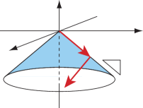
Figure 2: Projection onto the Coulomb friction cone.

In line 8 of Algorithm 2, we compute the projection of $\boldsymbol{s}_{j}\in\mathbb{R}^{3}$ onto the Coulomb friction cone $F$. This can be easily performed as follows.

For notational simplicity, we consider computation of $\Pi_{F}(s_{\mathrm{n}},\boldsymbol{s}_{\mathrm{t}})$, i.e., we omit subscript $j$. Define $\boldsymbol{\xi}_{1}$, $\boldsymbol{\xi}_{2}\in\mathbb{R}^{3}$ by

$$\boldsymbol{\xi}_{1}=-\frac{1}{1+\mu^{2}}\begin{bmatrix}\mu\\[4.30554pt] \displaystyle\frac{\boldsymbol{s}_{\mathrm{t}}}{\|\boldsymbol{s}_{\mathrm{t}}\|}\\ \end{bmatrix},\quad\boldsymbol{\xi}_{2}=\frac{1}{1+\mu^{2}}\begin{bmatrix}-1\\[4.30554pt] \displaystyle\mu\frac{\boldsymbol{s}_{\mathrm{t}}}{\|\boldsymbol{s}_{\mathrm{t}}\|}\\ \end{bmatrix};$$

see Figure 2. Also, define $\lambda_{1}$, $\lambda_{2}\in\mathbb{R}$ by

$$\lambda_{1}=-\mu s_{\mathrm{n}}-\|\boldsymbol{s}_{\mathrm{t}}\|,\quad\lambda_{2}=-s_{\mathrm{n}}+\mu\|\boldsymbol{s}_{\mathrm{t}}\|.$$

Then we have

$$\Pi_{F}(s_{\mathrm{n}},\boldsymbol{s}_{\mathrm{t}})=\max\{0,\lambda_{1}\}\boldsymbol{\xi}_{1}+\max\{0,\lambda_{2}\}\boldsymbol{\xi}_{2}.$$ (26)

It is worth noting that, when $\mu=1$, (26) corresponds to a formula of the projection onto the second-order cone [22] based on the spectral factorization in the Jordan algebra.

The computational procedure of the projection is described in Algorithm 3.

Algorithm 3 Projection onto the Coulomb’s friction cone, $\Pi_{F}(s_{\mathrm{n}},\boldsymbol{s}_{\mathrm{t}})$.

1:$(s_{\mathrm{n}},\boldsymbol{s}_{\mathrm{t}})\in\mathbb{R}\times\mathbb{R}^{2}$.

2:$\lambda_{1}\leftarrow-\mu s_{\mathrm{n}}-\|\boldsymbol{s}_{\mathrm{t}}\|$.

3:if $\lambda_{1}\geq 0$ then

4:     $\Pi_{F}(s_{\mathrm{n}},\boldsymbol{s}_{\mathrm{t}})\leftarrow(s_{\mathrm{n}},\boldsymbol{s}_{\mathrm{t}})$.

5:else

6:     $\lambda_{2}\leftarrow-s_{\mathrm{n}}+\mu\|\boldsymbol{s}_{\mathrm{t}}\|$.

7:     if  $\lambda_{2}\leq 0$  then

8:         $\Pi_{F}(s_{\mathrm{n}},\boldsymbol{s}_{\mathrm{t}})\leftarrow(0,\boldsymbol{0})$.

9:     else

10:         $\displaystyle\Pi_{F}(s_{\mathrm{n}},\boldsymbol{s}_{\mathrm{t}})\leftarrow\frac{\lambda_{2}}{1+\mu^{2}}\Bigl{(}-1,\mu\frac{\boldsymbol{s}_{\mathrm{t}}}{\|\boldsymbol{s}_{\mathrm{t}}\|}\Bigr{)}$.

11:     end if

12:end if

4 Numerical experiments

In this section, we demonstrate efficiency of the proposed method through numerical experiments. Section 4.1 describes details of implementation. Sections 4.2 and 4.3 report on two numerical examples. Computation was carried out on a 2.6 GHz Intel Core i7-9750H processor with 32 GB RAM. In the following, we omit units of physical quantities for simplicity. Young’s modulus and Poisson’s ratio of elastic bodies are $1$ and $0.3$, respectively.

4.1 Implementation

Algorithm 2 was implemented in Matlab ver. 9.8.0. Initial values were set to $\Delta\boldsymbol{u}^{(0)}=\boldsymbol{0}$, $\boldsymbol{r}^{(0)}=\boldsymbol{0}$, and $\alpha_{0}=10^{-1}$. Stopping criterion was $\|\Delta\boldsymbol{u}^{(k+1)}-\Delta\boldsymbol{u}^{(k)}\|\leq\epsilon$ with $\epsilon=10^{-12}$.

The projection onto the friction cone in line 8 is computed with Algorithm 3. Matlab implementation of Algorithm 3 was compiled into a MEX-file by using Matlab Coder, where the loop for $j=1,\dots,c$ was implemented with Matlab built-in function parfor. For this parallel loop computation, Matlab was allowed to use up to 6 cores.

As explained in section 3.3, a preconditioned conjugate gradient method was used for solution of a system of linear equations in line 10 of Algorithm 2. Matlab built-in function pcg was used, where the maximum number of iterations and the tolerance for termination were set to $10^{4}$ and $10^{-10}$, respectively. The minimum eigenvalue of $K$, i.e., $\mu_{\pi}$, was computed by eigs($\,\cdot\,$,1,’smallestabs’). The maximum singular value of $T$, i.e., $\sigma_{T}$, was computed by svds($\,\cdot\,$,1,’largest’), with setting the maximum number of iterations to $10^{8}$.

For comparison, the same problem instances were solved with a regularized and smoothed Newton method [24], which is implemented in ReSNA [23]. Specifically, we solved problem (31) in appendix A, which is a second-order cone linear complementarity problem. Parameter tole of ReSNA was set to $10^{-7}$. Both for ReSNA and Algorithm 2, the stiffness matrix $K$ was stored as a Matlab sparse form.

Besides computation time, we compare accuracy of the obtained solutions. With referring to problem (13), we consider the following three residuals. First, the residual of (13a) is

$$\|K\Delta\boldsymbol{u}^{(k)}-\boldsymbol{p}-T_{\mathrm{n}}\boldsymbol{r}_{\mathrm{n}}^{(k)}-T_{\mathrm{t}j}\boldsymbol{r}_{\mathrm{t}}^{(k)}\|.$$ (27)

Second, as the residual of the complementarity conditions in (13b), we consider

$$\left|\sum_{j=1}^{c}\left\langle\begin{bmatrix}-g_{j}-\mu\|T_{\mathrm{t}j}^{\top}\Delta\boldsymbol{u}^{(k)}\|+\boldsymbol{t}_{\mathrm{n}j}^{\top}\Delta\boldsymbol{u}^{(k)}\\ T_{\mathrm{t}j}^{\top}\Delta\boldsymbol{u}^{(k)}\\ \end{bmatrix},\begin{bmatrix}r_{\mathrm{n}j}^{(k)}\\ \boldsymbol{r}_{\mathrm{t}j}^{(k)}\\ \end{bmatrix}\right\rangle\right|=|\langle\boldsymbol{u}^{(k)},T\boldsymbol{r}^{(k)}\rangle-\langle\Delta\tilde{\boldsymbol{g}}^{(k)},\boldsymbol{r}_{\mathrm{n}}^{(k)}\rangle|.$$ (28)

Finally, for the inequality constraints $g_{j}-\boldsymbol{t}_{\mathrm{n}j}^{\top}\Delta\boldsymbol{u}\geq 0$ $(j=1,\dots,c)$ in (13b), the residual is

$$\|\min\{\boldsymbol{g}-T_{\mathrm{n}}^{\top}\Delta\boldsymbol{u}^{(k)},\boldsymbol{0}\}\|.$$ (29)

It is worth noting that $\boldsymbol{r}_{j}^{(k)}\in F$ $(j=1,\dots,c)$ is satisfied at every iteration of Algorithm 2, due to the projection in line 8.

4.2 Example (I): two-dimensional problem

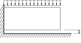
Figure 3: Problem setting of example (I).

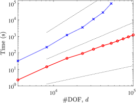
(a)

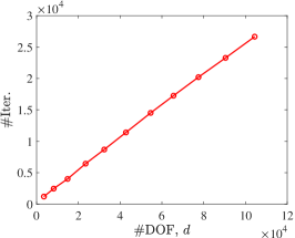
(b)

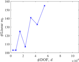
(c)

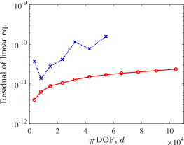
(d)

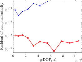
(e)

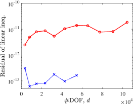
(f)

Figure 4: Computational results of example (I). “Solid line” The proposed method; and “dotted line” ReSNA. LABEL:sub@fig:time_log_dof_prog2ex_rev The computation time; LABEL:sub@fig:iter_pd_prog2ex_rev the number of iterations of the proposed method; LABEL:sub@fig:iter_soc_prog2ex_rev the number of systems of linear equations solved in ReSNA; LABEL:sub@fig:resid_eq_prog2ex_rev the residual in (27); LABEL:sub@fig:resid_compl_prog2ex_rev the residual in (28); and LABEL:sub@fig:resid_gap_ineq_prog2ex_rev the residual in (29).

Consider the problem outlined in Figure 3, where an elastic body is in the plane-stress state. The body is discretized uniformly as $N_{X}\times N_{Y}$ four-node quadrilateral (Q4) elements, where $N_{X}=2.5N_{Y}$ and the value of $N_{Y}$ is varied to change the size of problem instance. As for implementation of the finite element method, we use a Matlab code due to Andreassen et al. [5]. Uniformly distributed vertical traction of $0.01$ is applied at the top edge. The bottom nodes can possibly contact with a flat rigid obstacle. Hence, the number of contact candidate nodes is $c=N_{X}$. The initial gaps are set to $g_{j}=0.01$ $(j=1,\dots,c)$. The coefficient of friction is $\mu=0.5$.

Figure 4 collects the computational results for $N_{Y}=26$, 40, 54, 68, 80, 92, 104, 114, 124, 134, and 144. Here, “#DOF” means the number of degrees of freedom of the nodal displacements, i.e., $d$. Figure 4a shows the computation time. The dashed lines correspond to $O(d)$, $O(d^{2})$, and $O(d^{3})$. The proposed method clearly outperforms ReSNA in terms of computation time. For example, $382.6\,\mathrm{s}$ and $98222.0\,\mathrm{s}$ were required by the proposed method and ReSNA, respectively, to solve the instance with $d=54600$ and $c=260$. At the equilibrium state, about 40% contact candidate nodes are free, 10% are in sliding contact, and 50% are in sticking contact.

Figure 4b reports the number of iterations required by the proposed method. ReSNA solves a system of linear equations at step 2.1 of Algorithm 2 in [24], to obtain a search direction. Figure 4c reports the number of systems of linear equations solved at step 2.1. Increase of the number in Figure 4c is moderate compared with Figure 4b. Therefore, increase of computation time of ReSNA observed in Figure 4a may be due to increase of computation time for numerical solution of a system of linear equations at each iteration.

Figure 4d, Figure 4e, and Figure 4f compare the residuals defined by (27), (28), and (29), respectively. Concerning the residuals in (27) and (28), it is observed in Figure 4d and Figure 4e that the solution obtained by the proposed method has smaller residuals for every problem instance. In contrast, in terms of the residual in (29), the solution obtained by ReSNA has a smaller residual, although a residual of the solution obtained by the proposed method is also sufficiently small, as observed in Figure 4f.

4.3 Example (II): three-dimensional problem

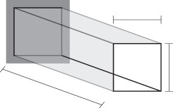
Figure 5: Problem setting of example (II).

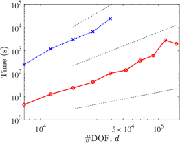
(a)

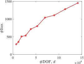
(b)

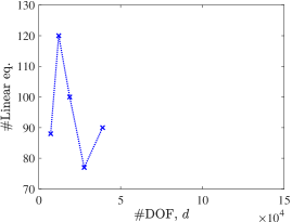
(c)

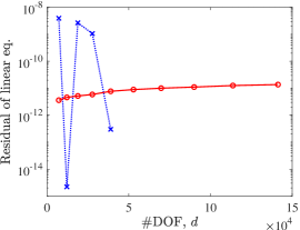
(d)

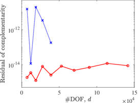
(e)

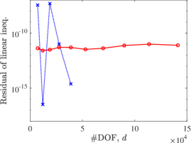
(f)

Figure 6: Computational results of example (II) with $\mu=0.5$. “Solid line” The proposed method; and “dotted line” ReSNA. LABEL:sub@fig:time_log_dof_prog4ex_rev The computation time; LABEL:sub@fig:iter_pd_prog4ex_rev the number of iterations of the proposed method; LABEL:sub@fig:iter_soc_prog4ex_rev the number of systems of linear equations solved in ReSNA; LABEL:sub@fig:resid_eq_prog4ex_rev the residual in (27); LABEL:sub@fig:resid_compl_prog4ex_rev the residual in (28); and LABEL:sub@fig:resid_gap_ineq_prog4ex_rev the residual in (29).

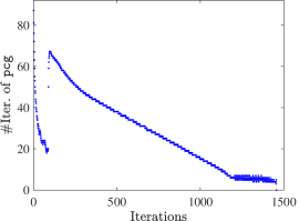
(a)

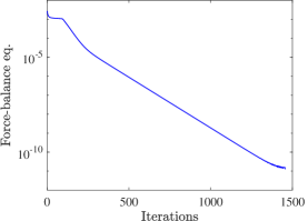
(b)

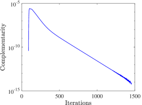
(c)

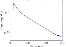
(d)

Figure 7: Iteration history of the proposed method for example (II) with $\mu=0.5$, $N_{X}=56$, $N_{Y}=N_{Z}=28$, $d=141288$, and $c=1624$. LABEL:sub@fig:prog4_pcg_iter The number of iterations of the conjugate gradient method; LABEL:sub@fig:prog4_resid_force_eq the residual in (27); LABEL:sub@fig:prog4_resid_comp the residual in (28); and LABEL:sub@fig:prog4_resid_gap_ineq the residual in (29).

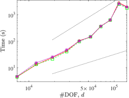
(a)

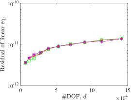
(b)

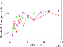
(c)

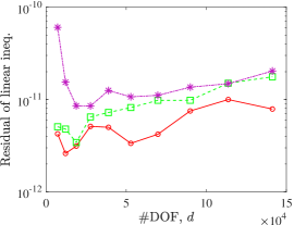
(d)

Figure 8: Computational results of the proposed method for example (II) with three different values of the friction coefficient. “Solid line” $\mu=0.5$; “dashed line” $\mu=1.0$; and “dashed-doted line” $\mu=1.5$. LABEL:sub@fig:time_log_dof_prog4ex_fric The computational time; LABEL:sub@fig:resid_eq_prog4ex_fric the residual in (27); LABEL:sub@fig:resid_compl_prog4ex_fric the residual in (28); and LABEL:sub@fig:resid_gap_ineq_prog4ex_fric the residual in (29).

Consider a three-dimensional version of example (I) outlined in Figure 5. The elastic body is discretized uniformly as $N_{X}\times N_{Y}\times N_{Z}$ 8-node hexahedron elements, where $N_{X}=2N_{Y}=2N_{Z}$. A Matlab code due to Ferrari and Sigmund [20] is used as for implementation of the finite element method. Uniformly distributed vertical traction of $5\times 10^{-3}$ is applied at all the top nodes. The bottom nodes are considered as contact candidate nodes, the number of which is $c=N_{X}(N_{Y}+1)$. The initial gaps are $g_{j}=0.005$ $(j=1,\dots,c)$. At the equilibrium state, about 33% contact candidate nodes are free, 11% are in sliding contact, and 56% are in sticking contact.

Figure 6 reports the computational results with $\mu=0.5$, where $N_{Y}=10$, 12, 14, 16, 18, 20, 22, 24, 26, and 28. It is observed in Figure 6a that the proposed method outperforms ReSNA from the viewpoint of computation time. Concerning the number of iterations, Figure 6b and Figure 6c show trends similar to the ones observed in example (I). From Figure 6d, Figure 6e, and Figure 6f we see that accuracy of the solutions obtained by the proposed method is comparable with that of the solutions obtained by ReSNA.

Figure 7 shows the iteration history of the proposed method. The number of iterations required by pcg for solving a system of linear equations in line 10 of Algorithm 2 decreases as the algorithm approaches to termination. The residual in (27) decreases monotonically. In contrast, the residuals in (28) and (29) are equal to zero for about the first 90 iterations. This is because the contact candidates nodes are free and have no reactions at these iterations as we set $\Delta\boldsymbol{u}^{(0)}=\boldsymbol{0}$ and $\boldsymbol{r}^{(0)}=\boldsymbol{0}$. The residuals become positive when the displacement violates the non-penetration condition, and then decrease monotonically.

For $\mu=0.5$, $1$, and $1.5$, Figure 8 compares performance of the proposed method. We can observe that the performance is irrelevant to a value of the friction coefficient.

5 Conclusions

This paper has developed a fast fist-order optimization-based method for a quasi-static contact problem with Coulomb’s friction. The method is designed based on an accelerated primal-dual algorithm solving a convex optimization problem that approximates the contact problem.

In the numerical experiments on problem instances with up to 140 thousands degrees of freedom of the nodal displacements, it has been observed that the proposed method successfully converges to a solution for every problem instance, although the method has no guarantee of convergence. Also, it has been demonstrated that the proposed method outperforms a regularized and smoothed Newton method for the second-order cone complementarity problem. Furthermore, the proposed method is easy to implement.

Acknowledgments

This work is supported by JSPS KAKENHI 17K06633, 21K04351, and JST CREST Grant No. JPMJCR1911, Japan.

Appendix A Formulation as second-order cone linear complementarity problem

ReSNA [23] is a Matlab software package implementing a regularized smoothing Newton method proposed by Hayashi et al. [24]. It solves a second-order cone linear complementarity problem (SOCLCP) in the following form:

$$\mathcal{K}\ni\boldsymbol{x}\perp\boldsymbol{y}\in\mathcal{K},$$ (30a)

$$\boldsymbol{y}=M_{11}\boldsymbol{x}+M_{12}\boldsymbol{v}+\boldsymbol{w}_{1},$$ (30b)

$$M_{21}\boldsymbol{x}+M_{22}\boldsymbol{v}+\boldsymbol{w}_{2}=\boldsymbol{0}.$$ (30c)

Here, $\boldsymbol{x}$, $\boldsymbol{y}$, and $\boldsymbol{v}$ are unknown variables, and $\mathcal{K}$ is a Cartesian product of some second-order cones. In the numerical experiments reported in section 4, we use ReSNA for comparison.

The method proposed in this paper attempts to solve problem (13) in section 2. Kanno et al. [31] showed that this problem can be recast as the following SOCLCP:

$$K\Delta\boldsymbol{u}=\boldsymbol{p}+T_{\mathrm{n}}\boldsymbol{r}_{\mathrm{n}}+T_{\mathrm{t}}\boldsymbol{r}_{\mathrm{t}},$$ (31a)

$$\mathbb{R}_{+}\ni(g_{j}-\boldsymbol{t}_{\mathrm{n}j}^{\top}\Delta\boldsymbol{u})\perp(-r_{\mathrm{n}j})\in\mathbb{R}_{+},\quad j=1,\dots,c,$$ (31b)

$$L^{3}\ni\begin{bmatrix}\lambda_{j}\\ T_{\mathrm{t}j}^{\top}\Delta\boldsymbol{u}\\ \end{bmatrix}\perp\begin{bmatrix}-\mu r_{\mathrm{n}j}\\ \boldsymbol{r}_{\mathrm{t}j}\\ \end{bmatrix}\in L^{3},\quad j=1,\dots,c.$$ (31c)

Here, $\mathbb{R}_{+}^{n}$ and $L^{n}$ are the nonnegative orthant and the second-order cone, respectively, i.e.,

$$\mathbb{R}_{+}^{n} =\{\boldsymbol{x}\in\mathbb{R}^{n}\mid\boldsymbol{x}\geq\boldsymbol{0}\},$$

$$L^{n} =\{(x_{0},\boldsymbol{x}_{1})\in\mathbb{R}\times\mathbb{R}^{n-1}\mid x_{0}\geq\|\boldsymbol{x}_{1}\|\},$$

and $\lambda_{j}\in\mathbb{R}$ $(j=1,\dots,c)$ are additional unknown variables.

Problem (31) can be embedded into the form of (30) as follows. Put

$$\boldsymbol{x}=\begin{bmatrix}\boldsymbol{g}-T_{\mathrm{n}}^{\top}\Delta\boldsymbol{u}\\ \lambda_{1}\\ T_{\mathrm{t}1}^{\top}\Delta\boldsymbol{u}\\ \vdots\\ \lambda_{c}\\ T_{\mathrm{t}c}^{\top}\Delta\boldsymbol{u}\\ \end{bmatrix},\quad\boldsymbol{y}=\begin{bmatrix}-\boldsymbol{r}_{\mathrm{n}}\\ -\mu r_{\mathrm{n}1}\\ \boldsymbol{r}_{\mathrm{t}1}\\ \vdots\\ -\mu r_{\mathrm{n}c}\\ \boldsymbol{r}_{\mathrm{t}c}\\ \end{bmatrix},\quad\boldsymbol{v}=\begin{bmatrix}\Delta\boldsymbol{u}\\ \boldsymbol{\lambda}\\ \boldsymbol{r}_{\mathrm{n}}\\ \boldsymbol{r}_{\mathrm{t}}\end{bmatrix}$$ (32)

to see that (31b) and (31c) are equivalently rewritten as (30a) with $\mathcal{K}\subset\mathbb{R}^{4c}$ defined by

$$\mathcal{K}=\mathbb{R}_{+}^{c}\times\mathcal{L}^{3}\times\dots\times\mathcal{L}^{3}.$$

Define $\boldsymbol{e}_{1}\in\mathbb{R}^{3}$ and $E_{2}\in\mathbb{R}^{3\times 2}$ by

$$\boldsymbol{e}_{1}=\begin{bmatrix}1\\ 0\\ 0\\ \end{bmatrix},\quad E_{2}=\begin{bmatrix}0&0\\ 1&0\\ 0&1\\ \end{bmatrix}.$$

We see that the relation between $\boldsymbol{y}$ and $\boldsymbol{v}$ in (32) can be written as

$$\boldsymbol{y} =M_{12}\boldsymbol{v}$$

with $M_{12}\in\mathbb{R}^{(4c)\times(d+4c)}$ defined by

$$M_{12}=\begin{bmatrix}O_{c,d}&O_{c,c}&-I_{c}&O_{c,2c}\\ O_{3c,d}&O_{3c,c}&-\mu I_{c}\otimes\boldsymbol{e}_{1}&I_{c}\otimes E_{2}\\ \end{bmatrix},$$ (33)

where we use $\otimes$ to denote the Kronecker product. Similarly, define $M_{22}^{(1)}\in\mathbb{R}^{(4c)\times(d+4c)}$ and $\boldsymbol{w}_{2}^{(1)}\in\mathbb{R}^{4c}$ by

$$M_{22}^{(1)}=\begin{bmatrix}T_{\mathrm{n}}^{\top}&O_{c,c}&O_{c,c}&O_{c,2c}\\ -(I_{c}\otimes E_{2})T_{\mathrm{t}}^{\top}&-I_{c}\otimes\boldsymbol{e}_{1}&O_{3c,c}&O_{3c,2c}\\ \end{bmatrix},\quad\boldsymbol{w}_{2}^{(1)}=\begin{bmatrix}-\boldsymbol{g}\\ O_{3c,1}\\ \end{bmatrix}$$

to see that the relation between $\boldsymbol{x}$ and $\boldsymbol{v}$ is reduced to

$$\boldsymbol{x}+M_{22}^{(1)}\boldsymbol{v}+\boldsymbol{w}_{2}^{(1)}=\boldsymbol{0}.$$

Furthermore, define $M_{22}^{(2)}\in\mathbb{R}^{d\times(d+4c)}$ and $\boldsymbol{w}_{2}^{(2)}\in\mathbb{R}^{d}$ by

$$M_{22}^{(2)}=\begin{bmatrix}K&O_{d,c}&-T_{\mathrm{n}}&-T_{\mathrm{t}}\\ \end{bmatrix},\quad\boldsymbol{w}_{2}^{(2)}=-\boldsymbol{p}.$$

Then we see that (31a) is reduced to

$$M_{22}^{(2)}\boldsymbol{v}+\boldsymbol{w}_{2}^{(2)}=\boldsymbol{0}.$$

Consequently, problem (31) can be transformed into the the form in (30) with

$$M_{11}=O_{4c,4c}, \boldsymbol{w}_{1}=O_{4c,1},$$

$$M_{21}=\begin{bmatrix}I_{4c}\\ O_{d,4c}\\ \end{bmatrix}, M_{22}=\begin{bmatrix}M_{22}^{(1)}\\ M_{22}^{(2)}\\ \end{bmatrix}, \boldsymbol{w}_{2}=\begin{bmatrix}\boldsymbol{w}_{2}^{(1)}\\ \boldsymbol{w}_{2}^{(2)}\\ \end{bmatrix},$$

and $M_{12}$ in (33).

Appendix B Optimality condition of problem (15)

We can confirm equivalence of (14) and (15) as follows.

Observe that problem (15) is written in an explicit manner as follows:

$$\mathop{\mathrm{Minimize}}_{\boldsymbol{u}\in\mathbb{R}^{d}} \frac{1}{2}\Delta\boldsymbol{u}^{\top}\,K\,\Delta\boldsymbol{u}-\boldsymbol{p}^{\top}\,\Delta\boldsymbol{u}$$ (34a)

$$\mathop{\mathrm{subject~{}to}} \begin{bmatrix}-\tilde{g}_{j}+\boldsymbol{t}_{\mathrm{n}j}^{\top}\,\Delta\boldsymbol{u}\\ T_{\mathrm{t}j}^{\top}\,\Delta\boldsymbol{u}\\ \end{bmatrix}\in F^{*},\quad j=1,\dots,c.$$ (34b)

Since $3c<d$, problem (34) has an interior feasible solution. The Lagrangian of problem (34) is defined by

$$L(\Delta\boldsymbol{u};\boldsymbol{r})=\begin{dcases*}\frac{1}{2}\Delta\boldsymbol{u}^{\top}\,K\,\Delta\boldsymbol{u}-\boldsymbol{p}^{\top}\,\Delta\boldsymbol{u}\\ \qquad{}-\sum_{j=1}^{c}\left\langle\begin{bmatrix}r_{\mathrm{n}j}\\ \boldsymbol{r}_{\mathrm{t}j}\\ \end{bmatrix},\begin{bmatrix}-\tilde{g}_{j}+\boldsymbol{t}_{\mathrm{n}j}^{\top}\,\Delta\boldsymbol{u}\\ T_{\mathrm{t}j}^{\top}\,\Delta\boldsymbol{u}\\ \end{bmatrix}\right\rangle&if $\begin{bmatrix}r_{\mathrm{n}j}\\ \boldsymbol{r}_{\mathrm{t}j}\\ \end{bmatrix}\in F$ $(j=1,\dots,c)$,\\ -\infty&otherwise.\end{dcases*}$$

Indeed, from the duality between $F$ and $F^{*}$ we see that problem (34) is equivalent to the following one:

$$\mathop{\mathrm{Minimize}}_{\Delta\boldsymbol{u}\in\mathbb{R}^{d}}\quad\sup_{\boldsymbol{r}\in\mathbb{R}^{3c}}L(\Delta\boldsymbol{u};\boldsymbol{r}).$$

Here, $\displaystyle\sup_{\boldsymbol{r}\in\mathbb{R}^{3c}}L(\Delta\boldsymbol{u};\boldsymbol{r})$ attains at a finite value if and only if (14b) is satisfied. Also, the stationarity condition of $L(\Delta\boldsymbol{u};\boldsymbol{r})$ with respect to $\Delta\boldsymbol{u}$ is (14a). Thus, (14) is a necessary and sufficient condition for optimality of problem (15).

References

- Acary et al. [2018] V. Acary, M. Brémond, and O. Huber: On solving contact problems with Coulomb friction: formulations and numerical comparisons. In R. I. Leine, V. Acary, O. Brüls (eds.): Advanced Topics in Nonsmooth Dynamics (Springer International Publishing, Cham, 2018), 375–457.
- Acary and Brogliato [2008] V. Acary and B. Brogliato: Numerical Methods for Nonsmooth Dynamical Systems (Springer-Verlag, Berlin, 2008).
- Acary et al. [2011] V. Acary, F. Cadoux, C. Lemaréchal, and J. Malick: A formulation of the linear discrete Coulomb friction problem via convex optimization. ZAMM, 91 (2011), 155–175.
- Alart and Curnier [1991] P. Alart and A. Curnier: A mixed formulation for frictional contact problems prone to Newton like solution methods. Computer Methods in Applied Mechanics and Engineering, 92 (1991), 353–375.
- Andreassen et al. [2011] E. Andreassen, A. Clausen, M. Schevenels, B. S. Lazarov, and O. Sigmund: Efficient topology optimization in MATLAB using 88 lines of code. Structural and Multidisciplinary Optimization, 43 (2011), 1–16.
- Areias et al. [2014] P. Areias, A. Pinto da Costa, T. Rabczuk, F. J. M. Queirós de Melo, D. Dias-da-Costa, and M. Bezzeghoud: An alternative formulation for quasi-static frictional and cohesive contact problems. Computational Mechanics, 53 (2014), 807–824.
- Bertails-Descoubes et al. [2011] F. Bertails-Descoubes, F. Cadoux, G. Daviet, and V. Acary: A nonsmooth Newton solver for capturing exact Coulomb friction in fiber assemblies. ACM Transactions of Graphics, 30 (2011), Article No. 6.
- Bonettini and Ruggiero [2012] S. Bonettini and V. Ruggiero: On the convergence of primal–dual hybrid gradient algorithms for total variation image restoration. Journal of Mathematical Imaging and Vision, 44 (2012), 236–253.
- Brogliato [2016] B. Brogliato: Nonsmooth Mechanics: Models, Dynamics and Control (3rd ed.) (Springer International Publishing, Cham, 2016).
- Cadoux [2009] F. Cadoux: An optimization-based algorithm for Coulomb’s frictional contact. ESAIM: Proceedings and Surveys, 27 (2009), 54–69.
- Chambolle and Pock [2011] A. Chambolle and T. Pock: A first-order primal-dual algorithm for convex problems with applications to imaging. Journal of Mathematical Imaging and Vision, 40 (2011), 120–145.
- Chambolle and Pock [2016a] A. Chambolle and T. Pock: An introduction to continuous optimization for imaging. Acta Numerica, 25 (2016), 161–319.
- Chambolle and Pock [2016b] A. Chambolle and T. Pock: On the ergodic convergence rates of a first-order primal–dual algorithm. Mathematical Programming, 159 (2016), 253–287.
- Chen et al. [2014] Y. Chen, G. Lan, and Y. Ouyang: Optimal primal-dual methods for a class of saddle point problems. SIAM Journal on Optimization, 24 (2014), 1779–1814.
- Chen and Pan [2012] J.-S. Chen and S. Pan: A survey on SOC complementarity functions and solution methods for SOCPs and SOCCPs. Pacific Journal of Optimization, 8 (2012), 33–74.
- Christensen [2002] P. W. Christensen: A semi-smooth Newton method for elasto-plastic contact problems. International Journal of Solids and Structures, 39 (2002), 2323–2341.
- Christensen et al. [1998] P. W. Christensen, A. Klarbring, J.-S. Pang, and N. Strömberg: Formulation and comparison of algorithms for frictional contact problems. International Journal for Numerical Methods in Engineering, 42 (1998), 145–173.
- Duvaut and Lions [1976] G. Duvaut and J. L. Lions: Inequalities in Mechanics and Physics (Springer-Verlag, Berlin, 1976).
- Esser et al. [2010] E. Esser, X. Zhang, and T. F. Chan: A general framework for a class of first order primal-dual algorithms for convex optimization in imaging science. SIAM Journal on Imaging Sciences, 3 (2010), 1015–1046.
- Ferrari and Sigmund [2020] F. Ferrari and O. Sigmund: A new generation 99 line Matlab code for compliance topology optimization and its extension to 3D. Structural and Multidisciplinary Optimization, 62 (2020), 2211–2228.
- Fujita and Kanno [2019] S. Fujita and Y. Kanno: Application of accelerated gradient method to equilibrium analysis of trusses with nonlinear elastic materials (in Japanese). Journal of Structural and Construction Engineering (Transactions of AIJ), 84 (2019), 1223–1230.
- Fukushima et al. [2001] M. Fukushima, Z.-Q. Luo, and P. Tseng: Smoothing functions for second-order-cone complementarity problems. SIAM Journal on optimization, 12 (2001), 436–460.
- Hayashi [2020] S. Hayashi: Website of ReSNA (Regularized Smoothing Newton Algorithm). http://optima.ws.hosei.ac.jp/hayashi/ReSNA/ (Accessed December 2020).
- Hayashi et al. [2005] S. Hayashi, N. Yamashita, and M. Fukushima: A combined smoothing and regularization method for monotone second-order cone complementarity problems. SIAM Journal on Optimization, 15 (2005), 593–615.
- He et al. [2014] B. He, Y. You, and X. Yuan: On the convergence of primal-dual hybrid gradient algorithm. SIAM Journal on Imaging Sciences, 7 (2014), 2526–2537.
- Kanno [2011] Y. Kanno: Nonsmooth Mechanics and Convex Optimization (CRC Press, Boca Raton, 2011).
- Kanno [2016] Y. Kanno: A fast first-order optimization approach to elastoplastic analysis of skeletal structures. Optimization and Engineering, 17 (2016), 861–896.
- Kanno [2020a] Y. Kanno: A note on a family of proximal gradient methods for quasi-static incremental problems in elastoplastic analysis. Theoretical and Applied Mechanics Letters, 10 (2020), 315–320.
- Kanno [2020b] Y. Kanno: An accelerated Uzawa method for application to frictionless contact problem. Optimization Letters, 14 (2020), 1845–1854.
- Kanno [to appear] Y. Kanno: Accelerated proximal gradient method for bi-modulus static elasticity. Optimization and Engineering, to appear. DOI:10.1007/s11081-021-09595-2
- Kanno et al. [2006] Y. Kanno, J. A. C. Martins, and A. Pinto da Costa: Three-dimensional quasi-static frictional contact by using second-order cone linear complementarity problem. International Journal for Numerical Methods in Engineering, 65 (2006), 62–83.
- Kikuchi and Oden [1988] N. Kikuchi and J. T. Oden: Contact Problems in Elasticity (SIAM, Philadelphia, 1988).
- Klarbring [1986] A. Klarbring: A mathematical programming approach to three-dimensional contact problems with friction. Computer Methods in Applied Mechanics and Engineering, 58 (1986), 175–200.
- Klarbring [1999] A. Klarbring: Contact, friction, discrete mechanical structures and mathematical programming. In P. Wriggers, P. Panagiotopoulos (eds.): New Developments in Contact Problems (Springer-Verlag, Wien, 1999), 55–100,
- Malitsky and Pock [2018] Y. Malitsky and T. Pock: A first-order primal-dual algorithm with linesearch. SIAM Journal on Optimization, 28 (2018), 411–432.
- Martins and Pinto da Costa [2000] J. M. C. Martins and A. Pinto da Costa: Stability of finite-dimensional nonlinear elastic systems with unilateral contact and friction. International Journal of Solids and Structures, 37 (2000), 2519–2564.
- Martins et al. [2002] J. A. C. Martins, A. Pinto da Costa, and F. M. F. Simões: Some notes on friction and instabilities. In J. A. C. Martins, M. Raous (eds.): Friction and Instabilities (Springer-Verlag, Wien, 2002), 65–136.
- Mazhar et al. [2015] H. Mazhar, T. Heyn, D, Negrut, and A. Tasora: Using Nesterov’s method to accelerate multibody dynamics with friction and contact. ACM Transactions on Graphics, 34 (2015), Article No. 32.
- Melanz et al. [2017] D. Melanz, L. Fang, P. Jayakumar, and D. Negrut: A comparison of numerical methods for solving multibody dynamics problems with frictional contact modeled via differential variational inequalities. Computer Methods in Applied Mechanics and Engineering, 320 (2017), 668–693.
- Pinto da Costa et al. [2004] A. Pinto da Costa, J. A. C. Martins, I. N. Figueiredo, and J. J. Júdice: The directional instability problem in systems with frictional contacts. Computer Methods in Applied Mechanics and Engineering, 193 (2004), 357–384.
- Renard [2013] Y. Renard: Generalized Newton’s methods for the approximation and resolution of frictional contact problems in elasticity. Computer Methods in Applied Mechanics and Engineering, 256 (2013), 38–55.
- Shimizu and Kanno [2018] W. Shimizu and Y. Kanno: Accelerated proximal gradient method for elastoplastic analysis with von Mises yield criterion. Japan Journal of Industrial and Applied Mathematics, 35 (2018), 1–32.
- Shimizu and Kanno [2020] W. Shimizu and Y. Kanno: A note on accelerated proximal gradient method for elastoplastic analysis with Tresca yield criterion. Journal of the Operations Research Society of Japan, 63 (2020), 78–92.
- Wriggers [2006] P. Wriggers: Computational Contact Mechanics (2nd ed.) (Springer-Verlag, Berlin, 2006).
- Yoshise [2012] A. Yoshise: Complementarity problems over symmetric cones: a survey of recent developments in several aspects. In M. F. Anjos, J. B. Lasserre (eds.): Handbook on Semidefinite, Conic and Polynomial Optimization (Springer, New York, 2012), 339–375.