Faster Kernel Interpolation for Gaussian Processes

Mohit Yadav Daniel Sheldon Cameron Musco
University of Massachusetts Amherst
{ymohit, sheldon, cmusco}@cs.umass.edu
Abstract

A key challenge in scaling Gaussian Process (GP) regression to massive datasets is that exact inference requires computation with a dense n×n𝑛𝑛n\times n kernel matrix, where n𝑛n is the number of data points. Significant work focuses on approximating the kernel matrix via interpolation using a smaller set of m𝑚m “inducing points”. Structured kernel interpolation (SKI) is among the most scalable methods: by placing inducing points on a dense grid and using structured matrix algebra, SKI achieves per-iteration time of 𝒪(n+mlogm)𝒪𝑛𝑚𝑚\mathcal{O}(n+m\log m) for approximate inference. This linear scaling in n𝑛n enables inference for very large data sets; however the cost is per-iteration, which remains a limitation for extremely large n𝑛n. We show that the SKI per-iteration time can be reduced to 𝒪(mlogm)𝒪𝑚𝑚\mathcal{O}(m\log m) after a single 𝒪(n)𝒪𝑛\mathcal{O}(n) time precomputation step by reframing SKI as solving a natural Bayesian linear regression problem with a fixed set of m𝑚m compact basis functions. With per-iteration complexity independent of the dataset size n𝑛n for a fixed grid, our method scales to truly massive data sets. We demonstrate speedups in practice for a wide range of m𝑚m and n𝑛n and apply the method to GP inference on a three-dimensional weather radar dataset with over 100 million points. Our code is available at https://github.com/ymohit/fkigp.

1 Introduction

GPs are a widely used and principled class of methods for predictive modeling. They have a long history in spatial statistics and geostatistics for spatio-temporal interpolation problems [16, 4]. They were later adopted in ML as general-purpose predictive models [26], motivated in part by connections to neural networks [20, 32]. More recently, similar connections have been identified between GPs and deep networks [15, 17, 8, 21, 3]. GPs can be used for general-purpose Bayesian regression [35, 25], classification [33], and many other applications [26, 36].

A well-known limitation of GPs is running-time scalability. The basic inference and learning tasks require linear algebraic operations (e.g., matrix inversion, linear solves, computing log-determinants) with an n×n𝑛𝑛n\times n kernel matrix, where n𝑛n is the number of data points. Exact computations require Θ(n3)Θsuperscript𝑛3\Theta(n^{3}) time — e.g., using the Cholesky decomposition — which severely limits applicability to large problems. Hence, a large amount of work has been devoted to improving scalability of GP inference and learning through approximation. Most of this work is based on the idea of forming an approximate kernel matrix that includes low-rank structure, e.g., through the use of inducing points or random features [34, 28, 23, 24, 13]. With rank-m𝑚m structure, the running time of key tasks can be reduced to Θ(nm2+m3)Θ𝑛superscript𝑚2superscript𝑚3\Theta(nm^{2}+m^{3}) [23]. However, this scaling with n𝑛n and m𝑚m continues to limit the size of input data sets that can be handled, the approximation accuracy, or both.

Structured kernel interpolation (SKI) is a promising approach to further improve the scalability of GP methods on relatively low-dimensional data [37]. In SKI, m𝑚m inducing points are placed on a regular grid, which, when combined with a stationary kernel covariance function, imposes extra structure in the approximate kernel matrix. Kernel matrix operations on the grid (i.e., multiplying with a vector) require only 𝒪(mlogm)𝒪𝑚𝑚\mathcal{O}(m\log m) time, and interpolating from the grid requires 𝒪(n)𝒪𝑛\mathcal{O}(n) time. By combining structured kernel operations with iterative methods for numerical linear algebra, the running time to solve core GP tasks becomes 𝒪(k(n+mlogm))𝒪𝑘𝑛𝑚𝑚\mathcal{O}(k(n+m\log m)) where k𝑘k is the number of iterations, and is usually much less than m𝑚m or n𝑛n. The modest per-iteration runtime of 𝒪(n+mlogm)𝒪𝑛𝑚𝑚\mathcal{O}(n+m\log m) allows the modeler to select a very large number of inducing points.

We show how to further improve the scalability of SKI with respect to n𝑛n and scale to truly massive data sets. We first show that the SKI approximation corresponds to exact inference in a Bayesian regression problem with a fixed set of m𝑚m compact spatial basis functions. This lets us reduce the per-iteration runtime to 𝒪(mlogm)𝒪𝑚𝑚\mathcal{O}(m\log m) — completely independent of n𝑛n — after a one-time preprocessing cost of 𝒪(n)𝒪𝑛\mathcal{O}(n) to compute sufficient statistics of the regression problem. However, naive application of these ideas introduces undesirable trade-offs: while the per-iteration cost is better, we must solve linear systems that are computationally less desirable than the original ones — e.g., they are asymmetric instead of symmetric, or have worse condition number. To avoid these trade-offs, we contribute novel “factorized" conjugate gradient and Lanczos methods, which allow us to solve the original linear systems in 𝒪(mlogm)𝒪𝑚𝑚\mathcal{O}(m\log m) time per-iteration instead of 𝒪(n+mlogm)𝒪𝑛𝑚𝑚\mathcal{O}(n+m\log m).

Our techniques accelerate SKI inference and learning across a wide range of settings. They apply to each of the main sub-tasks of GP inference: computing the posterior mean, posterior covariance, and log-likelihood. We demonstrate runtime improvements across different data sets and grid sizes, and the ability to scale GP inference to datasets well outside the typical range that can be handled by SKI or other approaches, such as inducing point methods. For example, we demonstrate the ability to perform GP inference on a three-dimensional weather radar dataset with 120120120 million data points, using a grid of 128,000128000128,000 inducing points.

1.1 Related Work

Outside of SKI and its variants [38, 7], a variety of scalable GP methods have been proposed. Most notable are inducing point methods (sparse GP approximations), such as the Nyström, SoRs, FITC, and SMGP methods [34, 28, 23, 31]. These methods require either Ω(nm2)Ω𝑛superscript𝑚2\Omega(nm^{2}) time for direct solves, or Ω(nm)Ω𝑛𝑚\Omega(nm) per-iteration cost if using iterative methods. Our approach significantly improves the dependence on both n𝑛n and m𝑚m to just 𝒪(n)𝒪𝑛\mathcal{O}(n) preprocessing time and 𝒪(mlogm)𝒪𝑚𝑚\mathcal{O}(m\log m) per-iteration cost.

While the above methods generally do not leverage structured matrix methods like SKI, especially in higher dimensions, they may achieve comparable accuracy with a smaller number of inducing points. Directly comparing SKI to popular inducing point methods is beyond the scope of this work, however prior work shows significant performance gains on large, relatively low-dimensional datasets [37, 5]. We note that very recent work [18] seeks to push the limits of inducing point methods via careful systems and hardware level implementations. Like our work, they scale to datasets with over 100 million points.

Many scalable GP methods have also been proposed in the geostatistics literature – see [11] for a survey. These include structured methods when observations lie on a grid [10, 29]. Most closely related to our work is fixed rank kriging (FRK) [4], which can be viewed as a generalization of our Bayesian regression interpretation of SKI. Like inducing point methods, FRK using m𝑚m basis functions requires Ω(nm2)Ω𝑛superscript𝑚2\Omega(nm^{2}) time. We show that SKI can be viewed as a special case of FRK with a fixed kernel function and a particular set of basis functions arising from interpolation. These two choices allow our faster runtime, through the application of structured matrix techniques and factorized iterative methods, which in turn significantly increases the number of basis functions that can be used.

2 Background

Notation: Throughout we use bold letters to represent vectors and capitals to represent matrices. In×n𝐼superscript𝑛𝑛I\in\mathbb{R}^{n\times n} represents the identity matrix, with dimension apparent from context. For Mp×r𝑀superscript𝑝𝑟M\in\mathbb{R}^{p\times r}, mv(M)𝑚𝑣𝑀mv(M) denotes the time required to multiply M𝑀M by any vector in rsuperscript𝑟\mathbb{R}^{r}.

2.1 Gaussian Process Regression

In GP regression [26], response values are modeled as noisy measurements of a random function f𝑓f on input data points. Let 𝒟𝒟\mathcal{D} be a set of n𝑛n points 𝐱1,,𝐱ndsubscript𝐱1subscript𝐱𝑛superscript𝑑\mathbf{x}_{1},\ldots,\mathbf{x}_{n}\in\mathbb{R}^{d} with corresponding response values y1,,ynsubscript𝑦1subscript𝑦𝑛y_{1},\ldots,y_{n}\in\mathbb{R}. Let 𝐲n𝐲superscript𝑛\mathbf{y}\in\mathbb{R}^{n} have its ithsuperscript𝑖𝑡i^{th} entry equal to yisubscript𝑦𝑖y_{i} and Xn×d𝑋superscript𝑛𝑑X\in\mathbb{R}^{n\times d} have its ithsuperscript𝑖𝑡i^{th} row equal to 𝐱isubscript𝐱𝑖\mathbf{x}_{i}. A Gaussian process with kernel (covariance) function k(𝐱,𝐱):d×d:𝑘𝐱superscript𝐱superscript𝑑superscript𝑑k(\mathbf{x},\mathbf{x}^{\prime}):\mathbb{R}^{d}\times\mathbb{R}^{d}\rightarrow\mathbb{R} is a random function f𝑓f such, for any 𝐱1,,𝐱ndsubscript𝐱1subscript𝐱𝑛superscript𝑑\mathbf{x}_{1},\ldots,\mathbf{x}_{n}\in\mathbb{R}^{d}:

𝐟=[f(𝐱1),,f(𝐱n)]𝒩(0,KX),𝐟𝑓subscript𝐱1𝑓subscript𝐱𝑛similar-to𝒩0subscript𝐾𝑋\displaystyle\mathbf{f}=[f(\mathbf{x}_{1}),...,f(\mathbf{x}_{n})]\sim\mathcal{N}(0,K_{X}), (1)

where KX=[k(𝐱i,𝐱j)]i,j=1nn×nsubscript𝐾𝑋superscriptsubscriptdelimited-[]𝑘subscript𝐱𝑖subscript𝐱𝑗𝑖𝑗1𝑛superscript𝑛𝑛K_{X}=[k(\mathbf{x}_{i},\mathbf{x}_{j})]_{i,j=1}^{n}\in\mathbb{R}^{n\times n} is the kernel (covariance) matrix on the data points X𝑋X. We assume without loss of generality that f𝑓f is zero-mean. The responses 𝐲𝐲\mathbf{y} are modeled as measurements of 𝐟Xsubscript𝐟𝑋\mathbf{f}_{X} with i.i.d. Gaussian noise, i.e., 𝐲𝒩(𝐟,σ2I)similar-to𝐲𝒩𝐟superscript𝜎2𝐼\mathbf{y}\sim\mathcal{N}(\mathbf{f},\sigma^{2}I).

The posterior distribution of f𝑓f given the data 𝒟=(X,𝐲)𝒟𝑋𝐲\mathcal{D}=(X,\mathbf{y}) is itself a Gaussian process. The standard GP inference tasks are to compute the posterior mean and covariance and the log-likelihood, given in Fact 1.

Fact 1 (Exact GP Inference).
The posterior mean, covariance, and log likelihood for Gaussian process regression are given by: mean: μf|𝒟(𝐱)=𝐤𝐱T𝐳mean: subscript𝜇conditional𝑓𝒟𝐱superscriptsubscript𝐤𝐱𝑇𝐳\displaystyle\textbf{mean: }\mu_{f|\mathcal{D}}(\mathbf{x})=\mathbf{k}_{\mathbf{x}}^{T}\mathbf{z} covariance: kf|𝒟(𝐱,𝐱)=k(𝐱,𝐱)𝐤𝐱T(KX+σ2I)1𝐤𝐱covariance: subscript𝑘conditional𝑓𝒟𝐱superscript𝐱𝑘𝐱superscript𝐱superscriptsubscript𝐤𝐱𝑇superscriptsubscript𝐾𝑋superscript𝜎2𝐼1subscript𝐤superscript𝐱\displaystyle\textbf{covariance: }k_{f|\mathcal{D}}(\mathbf{x},\mathbf{x}^{\prime})=k(\mathbf{x},\mathbf{x}^{\prime})-\mathbf{k}_{\mathbf{x}}^{T}({K}_{X}+\sigma^{2}I)^{-1}\mathbf{k}_{\mathbf{x}^{\prime}} log likelihood: logPr(𝐲)=12[logdet(KX+σ2I)+𝐲T𝐳+nlog(2π)]log likelihood: Pr𝐲12delimited-[]subscript𝐾𝑋superscript𝜎2𝐼superscript𝐲𝑇𝐳𝑛2𝜋\displaystyle\textbf{log likelihood: }\log\Pr(\mathbf{y})=-\frac{1}{2}[\log\det({K}_{X}+\sigma^{2}I)+\mathbf{y}^{T}\mathbf{z}+n\log(2\pi)] where 𝐤𝐱nsubscript𝐤𝐱superscript𝑛\mathbf{k}_{\mathbf{x}}\in\mathbb{R}^{n} has ithsuperscript𝑖𝑡i^{th} entry k(𝐱,𝐱i)𝑘𝐱subscript𝐱𝑖k(\mathbf{x},\mathbf{x}_{i}) and 𝐳=(KX+σ2I)1𝐲𝐳superscriptsubscript𝐾𝑋superscript𝜎2𝐼1𝐲\mathbf{z}=({K}_{X}+\sigma^{2}I)^{-1}\mathbf{y}.

Evaluating the posterior mean μf|𝒟(𝐱)subscript𝜇conditional𝑓𝒟𝐱\mu_{f|\mathcal{D}}(\mathbf{x}), covariance kf|𝒟(𝐱,𝐱)subscript𝑘conditional𝑓𝒟𝐱superscript𝐱k_{f|\mathcal{D}}(\mathbf{x},\mathbf{x}^{\prime}), and log likelihood require matrix-vector multiplication (MVM) with (KX+σ2I)1superscriptsubscript𝐾𝑋superscript𝜎2𝐼1({K}_{X}+\sigma^{2}I)^{-1}, which is the major run-time bottleneck for GP inference. Computing this inverse directly requires Θ(n3)Θsuperscript𝑛3\Theta(n^{3}) time. The log likelihood requires a further computation of logdet(KX+σ2I)subscript𝐾𝑋superscript𝜎2𝐼\log\det({K}_{X}+\sigma^{2}I), which again naively takes Θ(n3)Θsuperscript𝑛3\Theta(n^{3}) time using the Cholesky decomposition. Computing its gradient, which is necessary e.g., in hyper-parameter tuning with gradient based methods, requires a further trace computation involving (KX+σ2I)1superscriptsubscript𝐾𝑋superscript𝜎2𝐼1({K}_{X}+\sigma^{2}I)^{-1}.

Inference Via Iterative Methods.

One way to accelerate GP inference is to avoid full matrix factorization like Cholesky decomposition and instead use iterative methods. Gardner et al. [6] detail how to compute or approximate each term in Fact 1 using a modified version of the conjugate gradient (CG) algorithm.

For example, the vector 𝐳=(KX+σ2I)1𝐲n𝐳superscriptsubscript𝐾𝑋superscript𝜎2𝐼1𝐲superscript𝑛\mathbf{z}=({K}_{X}+\sigma^{2}I)^{-1}\mathbf{y}\in\mathbb{R}^{n} is computed by using CG to solve (KX+σ2I)𝐳=𝐲subscript𝐾𝑋superscript𝜎2𝐼𝐳𝐲({K}_{X}+\sigma^{2}I)\mathbf{z}=\mathbf{y}, which yields the posterior mean as μf|𝒟(𝐱)=𝐤𝐱T𝐳subscript𝜇conditional𝑓𝒟𝐱superscriptsubscript𝐤𝐱𝑇𝐳\mu_{f|\mathcal{D}}(\mathbf{x})=\mathbf{k}_{\mathbf{x}}^{T}\mathbf{z}, and is also used in the calculation of the log-likelihood.

We will use two iterative algorithms in our work: (1) conjugate gradient to solve linear systems A𝐯=𝐛𝐴𝐯𝐛A\mathbf{v}=\mathbf{b} for symmetric positive definite (SPD) A𝐴A, (2) the Lanczos algorithm to (sometimes partially) tridiagonalize an SPD matrix Ap×p𝐴superscript𝑝𝑝A\in\mathbb{R}^{p\times p} as A=QTQT𝐴𝑄𝑇superscript𝑄𝑇A=QTQ^{T} where Qp×p𝑄superscript𝑝𝑝Q\in\mathbb{R}^{p\times p} is orthonormal and Tp×p𝑇superscript𝑝𝑝T\in\mathbb{R}^{p\times p} is tridiagonal. Tridiagonalization is used to approximate logdet()\log\det(\cdot) terms [5, 30] and to compute a low-rank factorization for approximate posterior covariance evaluation [22].

Each iteration of CG or Lanczos for GP inference requires matrix-vector multiplication with A=KX+σ2I𝐴subscript𝐾𝑋superscript𝜎2𝐼A={K}_{X}+\sigma^{2}I, which in general takes mv(KX)+n=𝒪(n2)𝑚𝑣subscript𝐾𝑋𝑛𝒪superscript𝑛2mv(K_{X})+n=\mathcal{O}(n^{2}) time, but may be faster if KXsubscript𝐾𝑋K_{X} has special structure. The number of iterations required to reach a given error tolerance depends on eigenspectrum of A𝐴A, and is usually much less than n𝑛n, often on the order of 50 to 100. It can be even lower with preconditioning [6]. Recent work thus often informally considers the number of iterations to be a constant independent of n𝑛n.

2.2 Structured Kernel Interpolation

For large n𝑛n, the Θ(n2)Θsuperscript𝑛2\Theta(n^{2}) per-iteration cost of iterative methods is still prohibitively expensive. Structured kernel interpolation (SKI) is a method to accelerate MVMs by using an approximate kernel matrix with a special structure [37]. SKI approximates the kernel k(𝐱,𝐱)𝑘𝐱superscript𝐱k(\mathbf{x},\mathbf{x}^{\prime}) as:

k~(𝐱,𝐱)=𝐰𝐱TKG𝐰𝐱~𝑘𝐱superscript𝐱superscriptsubscript𝐰𝐱𝑇subscript𝐾𝐺subscript𝐰superscript𝐱\tilde{k}(\mathbf{x},\mathbf{x^{\prime}})=\mathbf{w}_{\mathbf{x}}^{T}K_{G}\mathbf{w}_{\mathbf{x}^{\prime}} (2)

where KGm×msubscript𝐾𝐺superscript𝑚𝑚K_{G}\in\mathbb{R}^{m\times m} is the kernel matrix for the set of m𝑚m points on a dense d𝑑d-dimensional grid, and the vector 𝐰𝐱msubscript𝐰𝐱superscript𝑚\mathbf{w}_{\mathbf{x}}\in\mathbb{R}^{m} contains interpolation weights to interpolate from grid points to arbitrary 𝐱d𝐱superscript𝑑\mathbf{x}\in\mathbb{R}^{d}. I.e., the kernel inner product between any two points is approximated by interpolating kernel inner products among grid points.

SKI can use any interpolation strategy (e.g., linear or cubic); typically, the strategy is local, so that 𝐰𝐱subscript𝐰𝐱\mathbf{w}_{\mathbf{x}} has only a constant number of non-zero entries corresponding to the grid points closest to 𝐱𝐱\mathbf{x}. E.g., for linear interpolation, 𝐰xsubscript𝐰𝑥\mathbf{w}_{x} has 2dsuperscript2𝑑2^{d} non-zeros. Let Wn×m𝑊superscript𝑛𝑚W\in\mathbb{R}^{n\times m} have ithsuperscript𝑖𝑡i^{th} row equal to 𝐰𝐱isubscript𝐰subscript𝐱𝑖\mathbf{w}_{\mathbf{x}_{i}}. SKI approximates the true kernel matrix KXsubscript𝐾𝑋K_{X} as K~X=WKGWTsubscript~𝐾𝑋𝑊subscript𝐾𝐺superscript𝑊𝑇\tilde{K}_{X}=WK_{G}W^{T}. Plugging this approximation directly into the GP inference equations of Fact 1 yields the SKI inference scheme in Def. 1.

Definition 1 (SKI Inference).
The SKI approximate inference equations are given by: mean: μf|𝒟(𝐱)𝐰𝐱TKGWT𝐳~mean: subscript𝜇conditional𝑓𝒟𝐱superscriptsubscript𝐰𝐱𝑇subscript𝐾𝐺superscript𝑊𝑇~𝐳\displaystyle\textbf{mean: }\mu_{f|\mathcal{D}}(\mathbf{x})\approx\mathbf{w}_{\mathbf{x}}^{T}K_{G}W^{T}\mathbf{\tilde{z}} covariance: kf|𝒟(𝐱,𝐱)𝐰𝐱TKG𝐰𝐱𝐤~𝐱T(K~X+σ2I)1𝐤~𝐱covariance: subscript𝑘conditional𝑓𝒟𝐱superscript𝐱superscriptsubscript𝐰𝐱𝑇subscript𝐾𝐺subscript𝐰superscript𝐱superscriptsubscript~𝐤𝐱𝑇superscriptsubscript~𝐾𝑋superscript𝜎2𝐼1subscript~𝐤𝐱\displaystyle\textbf{covariance: }k_{f|\mathcal{D}}(\mathbf{x},\mathbf{x}^{\prime})\approx\mathbf{w}_{\mathbf{x}}^{T}K_{G}\mathbf{w}_{\mathbf{x}^{\prime}}-\mathbf{\tilde{k}}_{\mathbf{x}}^{T}(\tilde{K}_{X}+\sigma^{2}I)^{-1}\mathbf{\tilde{k}}_{\mathbf{x}} log likelihood: logPr(𝐲)12[logdet(K~X+σ2I)+𝐲T𝐳~+nlog(2π)]log likelihood: Pr𝐲12delimited-[]subscript~𝐾𝑋superscript𝜎2𝐼superscript𝐲𝑇~𝐳𝑛2𝜋\displaystyle\textbf{log likelihood: }\log\Pr(\mathbf{y})\approx-\frac{1}{2}[\log\det(\tilde{K}_{X}+\sigma^{2}I)+\mathbf{y}^{T}\mathbf{\tilde{z}}+n\log(2\pi)] where K~X=WKGWTsubscript~𝐾𝑋𝑊subscript𝐾𝐺superscript𝑊𝑇\tilde{K}_{X}=WK_{G}W^{T} and 𝐳~=(K~X+σ2I)1𝐲~𝐳superscriptsubscript~𝐾𝑋superscript𝜎2𝐼1𝐲\mathbf{\tilde{z}}=\left(\tilde{K}_{X}+\sigma^{2}I\right)^{-1}\mathbf{y} and 𝐤~𝐱=WKG𝐰𝐱subscript~𝐤𝐱𝑊subscript𝐾𝐺subscript𝐰𝐱\mathbf{\tilde{k}}_{\mathbf{x}}=WK_{G}\mathbf{w}_{\mathbf{x}}.

SKI Running Time and Memory.

The SKI method admits efficient approximate inference due to: (1) the sparsity of the interpolation weight matrix W𝑊W, and (2) the structure of the on-grid kernel matrix KGsubscript𝐾𝐺K_{G}. The cost per iteration of CG or Lanczos is 𝒪(mv(K~X+σ2I))=𝒪(mv(W)+mv(KG)+n)𝒪𝑚𝑣subscript~𝐾𝑋superscript𝜎2𝐼𝒪𝑚𝑣𝑊𝑚𝑣subscript𝐾𝐺𝑛\mathcal{O}(mv(\tilde{K}_{X}+\sigma^{2}I))=\mathcal{O}(mv(W)+mv(K_{G})+n). This runtime is 𝒪(n+mlogm)𝒪𝑛𝑚𝑚\mathcal{O}(n+m\log m) per iteration assuming: (1) W𝑊W has 𝒪(1)𝒪1\mathcal{O}(1) entries per row and so mv(W)=𝒪(n)𝑚𝑣𝑊𝒪𝑛mv(W)=\mathcal{O}(n), and (2) KGsubscript𝐾𝐺K_{G} is multilevel Toeplitz, so mv(KG)=𝒪(mlogm)𝑚𝑣subscript𝐾𝐺𝒪𝑚𝑚mv(K_{G})=\mathcal{O}(m\log m) via fast Fourier transform [14]. The matrix KGsubscript𝐾𝐺K_{G} is multilevel Toeplitz (also known as block Toeplitz with Toeplitz blocks or BTTB) whenever G𝐺G is an equally-spaced grid and k(,)𝑘k(\cdot,\cdot) is stationary. The memory footprint is roughly 𝚗𝚗𝚣(W)+m+n=𝒪(n+m)𝚗𝚗𝚣𝑊𝑚𝑛𝒪𝑛𝑚\mathtt{nnz}(W)+m+n=\mathcal{O}(n+m) to store W𝑊W, KGsubscript𝐾𝐺K_{G}, and 𝐲𝐲\mathbf{y}, respectively, where 𝚗𝚗𝚣(A)𝚗𝚗𝚣𝐴\mathtt{nnz}(A) denotes the number of non zeros of A𝐴A.

Overall, the SKI per-iteration runtime of 𝒪(n+mlogm)𝒪𝑛𝑚𝑚\mathcal{O}(n+m\log m) significantly improves on the naive 𝒪(n2)𝒪superscript𝑛2\mathcal{O}(n^{2}) time required to apply the true kernel matrix KXsubscript𝐾𝑋K_{X}. However, when n𝑛n is very large, the 𝒪(n)𝒪𝑛\mathcal{O}(n) term (for both runtime and memory) can become a bottleneck. Our main contribution is to remove this cost, giving methods with 𝒪(mlogm)𝒪𝑚𝑚\mathcal{O}(m\log m) per-iteration runtime with 𝒪(m)𝒪𝑚\mathcal{O}(m) memory after 𝒪(n)𝒪𝑛\mathcal{O}(n) preprocessing.

3 SKI as Bayesian Linear Regression with Fixed Basis Functions

Our first contribution is to reformulate SKI as exact inference in a Bayesian linear regression problem with compact basis functions associated with grid points. This lets us use standard conjugate update formulas for Bayesian linear regression to reduce SKI’s per-iteration runtime to 𝒪(mlogm)𝒪𝑚𝑚\mathcal{O}(m\log m), with 𝒪(n)𝒪𝑛\mathcal{O}(n) preprocessing.

Refer to caption
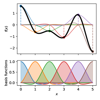
Figure 1: GSGP illustration. Bottom: basis functions for cubic interpolation are compact and centered at grid points. Top: a GSGP (thick black curve) is formed as the sum of scaled basis functions (lighter colored curves) with random weights at grid points (vertical dashed lines) drawn from the original GP.
Definition 2 (Grid-Structured Gaussian Process; GSGP).
Let G={𝐠1,,𝐠m}d𝐺subscript𝐠1subscript𝐠𝑚superscript𝑑G=\{\mathbf{g}_{1},\ldots,\mathbf{g}_{m}\}\subseteq\mathbb{R}^{d} be a set of grid points and k(𝐱,𝐱):d×d:𝑘𝐱superscript𝐱superscript𝑑superscript𝑑k(\mathbf{x},\mathbf{x}^{\prime}):\mathbb{R}^{d}\times\mathbb{R}^{d}\rightarrow\mathbb{R} be a positive-definite kernel function. A grid-structured Gaussian process f𝑓f is defined by the following generative process: 𝜽𝜽\displaystyle\boldsymbol{\theta} 𝒩(0,KG),similar-toabsent𝒩0subscript𝐾𝐺\displaystyle\sim\mathcal{N}(0,K_{G}), f(𝐱)𝑓𝐱\displaystyle f(\mathbf{x}) =𝐰𝐱T𝜽,𝐱d.formulae-sequenceabsentsuperscriptsubscript𝐰𝐱𝑇𝜽for-all𝐱superscript𝑑\displaystyle=\mathbf{w}_{\mathbf{x}}^{T}\boldsymbol{\theta},\quad\forall\mathbf{x}\in\mathbb{R}^{d}. where 𝐰xmsubscript𝐰𝑥superscript𝑚\mathbf{w}_{x}\in\mathbb{R}^{m} is a vector of interpolation weights from 𝐱𝐱\mathbf{x} to the grid G𝐺G.

Notice that a GSGP is a classical Bayesian linear regression model. In principle, 𝐰𝐰\mathbf{w} can be any mapping from dsuperscript𝑑\mathbb{R}^{d} to msuperscript𝑚\mathbb{R}^{m}. However, for computational efficiency and to match the notion of interpolation, the vector 𝐰𝐱subscript𝐰𝐱\mathbf{w}_{\mathbf{x}} will be taken to be the set of weights used by any fixed scheme to interpolate values from grid points to arbitrary locations 𝐱d𝐱superscript𝑑\mathbf{x}\in\mathbb{R}^{d}.

The generative process is illustrated in Figure 1 for d=1𝑑1d=1 and cubic interpolation on an integer grid [12]. The basis functions 𝐰𝐱jsubscriptsuperscript𝐰𝑗𝐱\mathbf{w}^{j}_{\mathbf{x}} for each grid point j𝑗j and for all 𝐱𝐱\mathbf{x} are shown in the bottom panel. The j𝑗jth basis function is centered at j𝑗j and supported on [j2,j+2)𝑗2𝑗2[j-2,j+2). For any fixed 𝐱𝐱\mathbf{x}, the vector 𝐰𝐱subscript𝐰𝐱\mathbf{w}_{\mathbf{x}} has at most four nonzero entries corresponding to the four nearest grid points.

The GSGP f𝑓f is generated by first drawing random weights 𝜽𝜽\boldsymbol{\theta} as the values of the original GP — with covariance function k(,)𝑘k(\cdot,\cdot) — at grid points. The generated function f(𝐱)𝑓𝐱f(\mathbf{x}) can be interpreted in two ways: (1) a sum of scaled basis functions f(𝐱)=j𝜽j𝐰𝐱j𝑓𝐱subscript𝑗subscript𝜽𝑗subscriptsuperscript𝐰𝑗𝐱f(\mathbf{x})=\sum_{j}\boldsymbol{\theta}_{j}\mathbf{w}^{j}_{\mathbf{x}}, (2) the result of interpolating the grid values 𝜽𝜽\boldsymbol{\theta} to dsuperscript𝑑\mathbb{R}^{d} using the interpolation scheme.

It is straightforward to verify the following (full derivations and proofs appear in Appendix A):

Claim 1.

A GSGP with grid weights 𝛉𝛉\boldsymbol{\theta} drawn from a GP with covariance function k(𝐱,𝐱)𝑘𝐱superscript𝐱k(\mathbf{x},\mathbf{x}^{\prime}) is itself a GP with covariance function k~(𝐱,𝐱)=𝐰𝐱TKG𝐰𝐱~𝑘𝐱superscript𝐱superscriptsubscript𝐰𝐱𝑇subscript𝐾𝐺subscript𝐰superscript𝐱\tilde{k}(\mathbf{x},\mathbf{x}^{\prime})=\mathbf{w}_{\mathbf{x}}^{T}K_{G}\mathbf{w}_{\mathbf{x}^{\prime}}.

In other words: the exact covariance function of the GSGP is the same as the SKI approximation in Eq. (2). Now, suppose noisy observations 𝐲𝒩(𝐟X,σ2)similar-to𝐲𝒩subscript𝐟𝑋superscript𝜎2\mathbf{y}\sim\mathcal{N}(\mathbf{f}_{X},\sigma^{2}) are made of the GSGP at input locations X𝑋X. It is well known that the posterior distribution of f𝑓f is a Gaussian process, with mean, covariance and log likelihood given in Fact 2 [19, 2]. From Claim 1 it follows that:

Theorem 1 (Equivalence of GSGP Inference and SKI Approximation).

The inference expressions of Fact 2 are identical to the SKI approximations of Def. 1.

Fact 2 (GSGP Inference).
The posterior mean, covariance, and log likelihood functions for the grid-structured Gaussian process (Def. 2) are given by: mean: μf|𝒟(𝐱)=𝐰𝐱T𝐳¯mean: subscript𝜇conditional𝑓𝒟𝐱superscriptsubscript𝐰𝐱𝑇¯𝐳\displaystyle\textbf{mean: }\mu_{f|\mathcal{D}}(\mathbf{x})=\mathbf{w}_{\mathbf{x}}^{T}\mathbf{\bar{z}} covariance: kf|𝒟(𝐱,𝐱)=𝐰𝐱T𝐂¯𝐰𝐱covariance: subscript𝑘conditional𝑓𝒟𝐱superscript𝐱superscriptsubscript𝐰𝐱𝑇¯𝐂subscript𝐰superscript𝐱\displaystyle\textbf{covariance: }k_{f|\mathcal{D}}(\mathbf{x},\mathbf{x}^{\prime})=\mathbf{w}_{\mathbf{x}}^{T}\mathbf{\bar{C}}\mathbf{w}_{\mathbf{x^{\prime}}} log likelihood: logPr(𝐲)=12[logdet(KGWTW+σ2I)+𝐲T(𝐲W𝐳¯)σ2+c],log likelihood: Pr𝐲12delimited-[]subscript𝐾𝐺superscript𝑊𝑇𝑊superscript𝜎2𝐼superscript𝐲𝑇𝐲𝑊¯𝐳superscript𝜎2𝑐\displaystyle\textbf{log likelihood: }\log\Pr(\mathbf{y})=-\frac{1}{2}\big{[}\log\det(K_{G}W^{T}W+\sigma^{2}I)+\frac{\mathbf{y}^{T}(\mathbf{y}-W\mathbf{\bar{z}})}{\sigma^{2}}+c\big{]}, where 𝐳¯=𝔼[𝛉|𝐲]=(KGWTW+σ2I)1KGWT𝐲¯𝐳𝔼delimited-[]conditional𝛉𝐲superscriptsubscript𝐾𝐺superscript𝑊𝑇𝑊superscript𝜎2𝐼1subscript𝐾𝐺superscript𝑊𝑇𝐲\mathbf{\bar{z}}=\mathbb{E}[\boldsymbol{\theta}|\mathbf{y}]=(K_{G}W^{T}W+\sigma^{2}I)^{-1}K_{G}W^{T}\mathbf{y} is the posterior mean of 𝛉𝛉\boldsymbol{\theta}, 𝐂¯=Var(𝛉|𝐲)=σ2(KGWTW+σ2I)1KG¯𝐂Varconditional𝛉𝐲superscript𝜎2superscriptsubscript𝐾𝐺superscript𝑊𝑇𝑊superscript𝜎2𝐼1subscript𝐾𝐺{\mathbf{\bar{C}}}=\operatorname{Var}(\boldsymbol{\theta}|\mathbf{y})=\sigma^{2}\left(K_{G}W^{T}W+\sigma^{2}I\right)^{-1}K_{G} is the posterior variance of 𝛉𝛉\boldsymbol{\theta} and c=nlog(2π)+(nm)logσ2𝑐𝑛2𝜋𝑛𝑚superscript𝜎2c=n\log(2\pi)+(n-m)\log\sigma^{2}.

3.1 GSGP Running Time and Memory

By Theorem 1, we can apply the SKI approximation using the GSGP inference equations of Fact 2; these also involve structured matrices that are well suited to iterative methods. In particular, they require linear solves and logdet computation for the m×m𝑚𝑚m\times m matrix KGWTW+σ2Isubscript𝐾𝐺superscript𝑊𝑇𝑊superscript𝜎2𝐼K_{G}W^{T}W+\sigma^{2}I rather than the n×n𝑛𝑛n\times n matrix WKGWT+σ2I𝑊subscript𝐾𝐺superscript𝑊𝑇superscript𝜎2𝐼WK_{G}W^{T}+\sigma^{2}I. Under the standard SKI assumptions, this leads to 𝒪(mlogm)𝒪𝑚𝑚\mathcal{O}(m\log m) per-iteration run time and 𝒪(m)𝒪𝑚\mathcal{O}(m) memory footprint with 𝒪(n)𝒪𝑛\mathcal{O}(n) precomputation.

Precomputation: GSGP involves precomputing WTWm×msuperscript𝑊𝑇𝑊superscript𝑚𝑚W^{T}W\in\mathbb{R}^{m\times m}, WT𝐲msuperscript𝑊𝑇𝐲superscript𝑚W^{T}\mathbf{y}\in\mathbb{R}^{m}, and 𝐲T𝐲superscript𝐲𝑇𝐲\mathbf{y}^{T}\mathbf{y}\in\mathbb{R}, which are the sufficient statistics of a linear regression problem with feature matrix W𝑊W. Each is a sum over n𝑛n data points and has fixed size depending only on m𝑚m. Once computed, each expression in Fact 2 can be computed without referring back to the data W𝑊W and 𝐲𝐲\mathbf{y}.

It is clear that 𝐲T𝐲=i=1nyi2superscript𝐲𝑇𝐲superscriptsubscript𝑖1𝑛superscriptsubscript𝑦𝑖2\mathbf{y}^{T}\mathbf{y}=\sum_{i=1}^{n}y_{i}^{2} can be computed in 𝒪(n)𝒪𝑛\mathcal{O}(n) time with a single pass over the data. Assume the interpolation strategy is local (e.g., linear or cubic interpolation), so that each 𝐰𝐱isubscript𝐰subscript𝐱𝑖\mathbf{w}_{\mathbf{x}_{i}} has 𝒪(1)𝒪1\mathcal{O}(1) non-zeros. Then WT𝐲=i=1n𝐰𝐱iT𝐲superscript𝑊𝑇𝐲superscriptsubscript𝑖1𝑛superscriptsubscript𝐰subscript𝐱𝑖𝑇𝐲W^{T}\mathbf{y}=\sum_{i=1}^{n}\mathbf{w}_{\mathbf{x}_{i}}^{T}\mathbf{y} can also be computed in 𝒪(n)𝒪𝑛\mathcal{O}(n) time with one pass over the data, since each inner product accesses only a constant number of entries of 𝐲𝐲\mathbf{y}. WTWsuperscript𝑊𝑇𝑊W^{T}W also has desirable computational properties:

Claim 2.

Assume that G={𝐠1,,𝐠m}𝐺subscript𝐠1subscript𝐠𝑚G=\{\mathbf{g}_{1},\ldots,\mathbf{g}_{m}\} has spacing s𝑠s, i.e., 𝐠i𝐠jssubscriptdelimited-∥∥subscript𝐠𝑖subscript𝐠𝑗𝑠\left\lVert\mathbf{g}_{i}-\mathbf{g}_{j}\right\rVert_{\infty}\geq s for any i,jm𝑖𝑗𝑚i,j\in m and that 𝐰𝐱jsubscriptsuperscript𝐰𝑗𝐱\mathbf{w}^{j}_{\mathbf{x}} is non-zero only if 𝐠j𝐱<rssubscriptnormsubscript𝐠𝑗𝐱𝑟𝑠\|\mathbf{g}_{j}-\mathbf{x}\|_{\infty}<r\cdot s for some fixed integer r𝑟r. Then WTWsuperscript𝑊𝑇𝑊W^{T}W can be computed in 𝒪(n(2r)2d)𝒪𝑛superscript2𝑟2𝑑\mathcal{O}(n(2r)^{2d}) time and has at most (4r1)dsuperscript4𝑟1𝑑(4r-1)^{d} entries per row. Therefore mv(WTW)=𝒪(m(4r1)d).𝑚𝑣superscript𝑊𝑇𝑊𝒪𝑚superscript4𝑟1𝑑mv(W^{T}W)=\mathcal{O}(m(4r-1)^{d}).

For example, r=1𝑟1r=1 for linear interpolation and r=2𝑟2r=2 for cubic interpolation. The upshot is that WTWsuperscript𝑊𝑇𝑊W^{T}W can be precomputed in 𝒪(n)𝒪𝑛\mathcal{O}(n) time, after which matrix-vector multiplications take 𝒪(m)𝒪𝑚\mathcal{O}(m) time, with dependence on r𝑟r and d𝑑d similar to that of mv(W)=𝒪(n(2r)d)𝑚𝑣𝑊𝒪𝑛superscript2𝑟𝑑mv(W)=\mathcal{O}(n(2r)^{d}).

Per-Iteration and Memory: As discussed in Section 2.2, due to its grid structure, KGsubscript𝐾𝐺K_{G} admits fast matrix-vector multiplication: mv(KG)=𝒪(mlogm)𝑚𝑣subscript𝐾𝐺𝒪𝑚𝑚mv(K_{G})=\mathcal{O}(m\log m) for stationary kernels. Since WTWsuperscript𝑊𝑇𝑊W^{T}W is sparse, mv(WTW)=𝒪(m)𝑚𝑣superscript𝑊𝑇𝑊𝒪𝑚mv(W^{T}W)=\mathcal{O}(m). Overall, mv(KGWTW+σ2I)=𝒪(mlogm)𝑚𝑣subscript𝐾𝐺superscript𝑊𝑇𝑊superscript𝜎2𝐼𝒪𝑚𝑚mv(K_{G}W^{T}W+\sigma^{2}I)=\mathcal{O}(m\log m), giving per-iteration runtime of 𝒪(mlogm)𝒪𝑚𝑚\mathcal{O}(m\log m) for computing the approximate mean, covariance, and log-likelihood in Fact 2 via iterative methods. Importantly, this complexity is independent of the number of data points n𝑛n. GSGP uses 𝚗𝚗𝚣(WTW)+m+m=𝒪(m)𝚗𝚗𝚣superscript𝑊𝑇𝑊𝑚𝑚𝒪𝑚\mathtt{nnz}(W^{T}W)+m+m=\mathcal{O}(m) memory to store WTWsuperscript𝑊𝑇𝑊W^{T}W, WT𝐲superscript𝑊𝑇𝐲W^{T}\mathbf{y} and KGsubscript𝐾𝐺K_{G}.

Limitations of GSGP.

Directly replacing the classic SKI method with the GSGP inference equations of Fact 2 reduces per-iteration cost but has some undesirable trade-offs. In particular, unlike WKGWT+σ2I𝑊subscript𝐾𝐺superscript𝑊𝑇superscript𝜎2𝐼WK_{G}W^{T}+\sigma^{2}I, the matrix KGWTW+σ2Isubscript𝐾𝐺superscript𝑊𝑇𝑊superscript𝜎2𝐼K_{G}W^{T}W+\sigma^{2}I is asymmetric. Thus, conjugate gradient and Lanczos—which are designed for symmetric positive semidefinite matrices—are not applicable. Asymmetric solvers like GMRES [27] can be used, and seem to work well in practice for posterior mean estimation, but do not enjoy the same theoretical convergence guarantees, nor do they as readily provide the approximate tridiagonalization for low-rank approximation for predictive covariance [22] or log-likelihood estimation [5]. It is possible to algebraically manipulate the GSGP expressions to yield symmetric m×m𝑚𝑚m\times m systems, but these lose the desirable ‘regularized form’ A+σ2I𝐴superscript𝜎2𝐼A+\sigma^{2}I and have worse conditioning, leading to more iterations being required in practice (see Appendix A).

4 Efficient SKI via Factorized Iterative Methods

In this section we show how to achieve the best of both SKI and the GSGP reformulation: we design ‘factorized’ versions of the CG and Lanczos methods used in SKI with just 𝒪(mlogm)𝒪𝑚𝑚\mathcal{O}(m\log m) per-iteration complexity. These methods are mathematically equivalent to the full methods, and so enjoy identical convergence rates, avoiding the complications of the asymmetric solves required by GSGP inference.

4.1 The Factorized Approach

Our approach centers on a simple observation relating matrix-vector multiplication with the SKI kernel approximation K~X=WKGWT+σ2Isubscript~𝐾𝑋𝑊subscript𝐾𝐺superscript𝑊𝑇superscript𝜎2𝐼\tilde{K}_{X}=WK_{G}W^{T}+\sigma^{2}I and the GSGP operator KGWTW+σ2Isubscript𝐾𝐺superscript𝑊𝑇𝑊superscript𝜎2𝐼K_{G}W^{T}W+\sigma^{2}I. To apply the SKI equations of Def. 1 via an iterative method, a key step at each iteration is to multiply some iterate 𝐳insubscript𝐳𝑖superscript𝑛\mathbf{z}_{i}\in\mathbb{R}^{n} by K~Xsubscript~𝐾𝑋\tilde{K}_{X}, requiring 𝒪(n+mlogm)𝒪𝑛𝑚𝑚\mathcal{O}(n+m\log m) time. We avoid this by maintaining a compressed representation of any iterate as 𝐳i=W𝐳^i+ci𝐳0subscript𝐳𝑖𝑊subscript^𝐳𝑖subscript𝑐𝑖subscript𝐳0\mathbf{z}_{i}=W\mathbf{\hat{z}}_{i}+c_{i}\mathbf{z}_{0}, where 𝐳^imsubscript^𝐳𝑖superscript𝑚\mathbf{\hat{z}}_{i}\in\mathbb{R}^{m}, cisubscript𝑐𝑖c_{i}\in\mathbb{R} is a scalar coefficient, and 𝐳0subscript𝐳0\mathbf{z}_{0} is an initial value. At initialization, 𝐳^0=𝟎subscript^𝐳00\mathbf{\hat{z}}_{0}=\mathbf{0} and c0=1subscript𝑐01c_{0}=1. Critically, this compressed representation can be updated with multiplication by K~Xsubscript~𝐾𝑋\tilde{K}_{X} in just 𝒪(mlogm)𝒪𝑚𝑚\mathcal{O}(m\log m) time using the following claim:

Claim 3 (Factorized Matrix-Vector Multiplication).

For any 𝐳insubscript𝐳𝑖superscript𝑛\mathbf{z}_{i}\in\mathbb{R}^{n} with 𝐳i=W𝐳^i+ci𝐳0subscript𝐳𝑖𝑊subscript^𝐳𝑖subscript𝑐𝑖subscript𝐳0\mathbf{z}_{i}=W\mathbf{\hat{z}}_{i}+c_{i}\mathbf{z}_{0},

(WKGWT+σ2I)𝐳i=W𝐳^i+1+ci+1𝐳0,𝑊subscript𝐾𝐺superscript𝑊𝑇superscript𝜎2𝐼subscript𝐳𝑖𝑊subscript^𝐳𝑖1subscript𝑐𝑖1subscript𝐳0\displaystyle(WK_{G}W^{T}+\sigma^{2}I)\mathbf{z}_{i}=W\mathbf{\hat{z}}_{i+1}+c_{i+1}\mathbf{z}_{0},

where 𝐳^i+1=(KGWTW+σ2I)𝐳^i+ciKGWT𝐳0subscript^𝐳𝑖1subscript𝐾𝐺superscript𝑊𝑇𝑊superscript𝜎2𝐼subscript^𝐳𝑖subscript𝑐𝑖subscript𝐾𝐺superscript𝑊𝑇subscript𝐳0\mathbf{\hat{z}}_{i+1}=(K_{G}W^{T}W+\sigma^{2}I)\mathbf{\hat{z}}_{i}+c_{i}K_{G}W^{T}\mathbf{z}_{0} and ci+1=σ2cisubscript𝑐𝑖1superscript𝜎2subscript𝑐𝑖c_{i+1}=\sigma^{2}\cdot c_{i}. Call this operation a factorized update and denote it as (𝐳^i+1,ci+1)=𝒜(𝐳^i,ci)subscript^𝐳𝑖1subscript𝑐𝑖1𝒜subscript^𝐳𝑖subscript𝑐𝑖(\mathbf{\hat{z}}_{i+1},c_{i+1})=\mathcal{A}(\mathbf{\hat{z}}_{i},c_{i}). If the vector KGWT𝐳0subscript𝐾𝐺superscript𝑊𝑇subscript𝐳0K_{G}W^{T}\mathbf{z}_{0} is precomputed in 𝒪(n+mlogm)𝒪𝑛𝑚𝑚\mathcal{O}(n+m\log m) time, each subsequent factorized update takes 𝒪(mlogm)𝒪𝑚𝑚\mathcal{O}(m\log m) time.

For algorithms such as CG we also need to support additions and inner products in the compressed representation. Additions are simple via linearity. Inner products can be computed efficiently as well:

Claim 4 (Factorized Inner Products).

For any 𝐳i,𝐲insubscript𝐳𝑖subscript𝐲𝑖superscript𝑛\mathbf{z}_{i},\mathbf{y}_{i}\in\mathbb{R}^{n} with 𝐳i=W𝐳^i+ci𝐳0subscript𝐳𝑖𝑊subscript^𝐳𝑖subscript𝑐𝑖subscript𝐳0\mathbf{z}_{i}=W\mathbf{\hat{z}}_{i}+c_{i}\mathbf{z}_{0} and 𝐲i=W𝐲^i+di𝐲0subscript𝐲𝑖𝑊subscript^𝐲𝑖subscript𝑑𝑖subscript𝐲0\mathbf{y}_{i}=W\mathbf{\hat{y}}_{i}+d_{i}\mathbf{y}_{0},

𝐳iT𝐲isuperscriptsubscript𝐳𝑖𝑇subscript𝐲𝑖\displaystyle\mathbf{z}_{i}^{T}\mathbf{y}_{i} =𝐳^iTWTW𝐲^i+di𝐳^iTWT𝐲0absentsuperscriptsubscript^𝐳𝑖𝑇superscript𝑊𝑇𝑊subscript^𝐲𝑖subscript𝑑𝑖superscriptsubscript^𝐳𝑖𝑇superscript𝑊𝑇subscript𝐲0\displaystyle=\mathbf{\hat{z}}_{i}^{T}W^{T}W\mathbf{\hat{y}}_{i}+d_{i}\mathbf{\hat{z}}_{i}^{T}W^{T}\mathbf{y}_{0}
+ci𝐲^iTWT𝐳0+cidi𝐲0T𝐳0.subscript𝑐𝑖superscriptsubscript^𝐲𝑖𝑇superscript𝑊𝑇subscript𝐳0subscript𝑐𝑖subscript𝑑𝑖superscriptsubscript𝐲0𝑇subscript𝐳0\displaystyle+c_{i}\mathbf{\hat{y}}_{i}^{T}W^{T}\mathbf{z}_{0}+c_{i}d_{i}\mathbf{y}_{0}^{T}\mathbf{z}_{0}.

We denote the above operation by (𝐳^i,ci),(𝐲^i,di)subscript^𝐳𝑖subscript𝑐𝑖subscript^𝐲𝑖subscript𝑑𝑖\langle(\mathbf{\hat{z}}_{i},c_{i}),(\mathbf{\hat{y}}_{i},d_{i})\rangle. If WT𝐳0superscript𝑊𝑇subscript𝐳0{W}^{T}\mathbf{z}_{0}, WT𝐲0superscript𝑊𝑇subscript𝐲0{W}^{T}\mathbf{y}_{0}, and 𝐲0T𝐳0superscriptsubscript𝐲0𝑇subscript𝐳0\mathbf{y}_{0}^{T}\mathbf{z}_{0} are precomputed in 𝒪(n)𝒪𝑛\mathcal{O}(n) time, then (𝐳^i,ci),(𝐲^i,di)subscript^𝐳𝑖subscript𝑐𝑖subscript^𝐲𝑖subscript𝑑𝑖\langle(\mathbf{\hat{z}}_{i},c_{i}),(\mathbf{\hat{y}}_{i},d_{i})\rangle can be computed using just one matrix-vector multiplication with WTWsuperscript𝑊𝑇𝑊W^{T}W and 𝒪(m)𝒪𝑚\mathcal{O}(m) additional time.

4.2 Factorized Conjugate Gradient

We now give an example of this approach by deriving a “factorized conjugate gradient” algorithm. Factorized CG has lower per-iteration complexity than standard CG for computing the posterior mean, covariance, and log likelihood in the SKI approximations of Def. 1. In Appendix B we apply the same approach to the Lanczos method, which can be used in approximating the logdet term in the log likelihood, and for computing a low-rank approximation of the posterior covariance.

Figure 2 shows a side by side of the classic CG method and our factorized variant. CG maintains three iterates, the current solution estimate 𝐱ksubscript𝐱𝑘\mathbf{x}_{k}, the residual 𝐫ksubscript𝐫𝑘\mathbf{r}_{k}, and a search direction 𝐩ksubscript𝐩𝑘\mathbf{p}_{k}. We maintain each in a compressed form with 𝐱k=W𝐱^k+ckx𝐫0+𝐱0subscript𝐱𝑘𝑊subscript^𝐱𝑘superscriptsubscript𝑐𝑘𝑥subscript𝐫0subscript𝐱0\mathbf{x}_{k}=W\mathbf{\hat{x}}_{k}+c_{k}^{x}\mathbf{r}_{0}+\mathbf{x}_{0}, 𝐫k=W𝐫^k+ckr𝐫0subscript𝐫𝑘𝑊subscript^𝐫𝑘superscriptsubscript𝑐𝑘𝑟subscript𝐫0\mathbf{r}_{k}=W\mathbf{\hat{r}}_{k}+c_{k}^{r}\mathbf{r}_{0}, and 𝐩k=W𝐩^k+ckp𝐫0subscript𝐩𝑘𝑊subscript^𝐩𝑘superscriptsubscript𝑐𝑘𝑝subscript𝐫0\mathbf{p}_{k}=W\mathbf{\hat{p}}_{k}+c_{k}^{p}\mathbf{r}_{0}. Note that the initialization term 𝐫0subscript𝐫0\mathbf{r}_{0} is shared across all iterates with a different coefficient, and that 𝐱ksubscript𝐱𝑘\mathbf{x}_{k} has an additional fixed component 𝐱0subscript𝐱0\mathbf{x}_{0}. This is an initial solution guess for the system solve, frequently zero. With these invariants, simply applying Claims 3 and 4 gives the factorized algorithm.

Algorithm 1 Conjugate gradient
1:procedure CG(KG,W,𝐛,σ,𝐱0,ϵsubscript𝐾𝐺𝑊𝐛𝜎subscript𝐱0italic-ϵK_{G},W,\mathbf{b},\sigma,\mathbf{x}_{0},\epsilon)
2:     𝐫0=𝐛K~𝐱0subscript𝐫0𝐛~𝐾subscript𝐱0\mathbf{r}_{0}=\mathbf{b}-\tilde{K}\mathbf{x}_{0}
3:     𝐩0=𝐫0subscript𝐩0subscript𝐫0\mathbf{p}_{0}=\mathbf{r}_{0}
4:     for k=0𝑘0k=0 to maxiter do
5:         αk=𝐫kT𝐫k𝐩kTK~𝐩ksubscript𝛼𝑘superscriptsubscript𝐫𝑘𝑇subscript𝐫𝑘superscriptsubscript𝐩𝑘𝑇~𝐾subscript𝐩𝑘\alpha_{k}={\frac{\mathbf{r}_{k}^{T}\mathbf{r}_{k}}{\mathbf{p}_{k}^{T}\tilde{K}\mathbf{p}_{k}}}
6:         𝐱k+1=𝐱k+αk𝐩ksubscript𝐱𝑘1subscript𝐱𝑘subscript𝛼𝑘subscript𝐩𝑘\mathbf{x}_{k+1}=\mathbf{x}_{k}+\alpha_{k}\cdot\mathbf{p}_{k}
7:         𝐫k+1=𝐫kαkK~𝐩ksubscript𝐫𝑘1subscript𝐫𝑘subscript𝛼𝑘~𝐾subscript𝐩𝑘\mathbf{r}_{k+1}=\mathbf{r}_{k}-\alpha_{k}\cdot\tilde{K}\mathbf{p}_{k}
8:         if 𝐫k+1T𝐫k+1ϵsuperscriptsubscript𝐫𝑘1𝑇subscript𝐫𝑘1italic-ϵ\mathbf{r}_{k+1}^{T}\mathbf{r}_{k+1}\leq\epsilon exit loop
9:         βk=𝐫k+1T𝐫k+1𝐫kT𝐫ksubscript𝛽𝑘superscriptsubscript𝐫𝑘1𝑇subscript𝐫𝑘1superscriptsubscript𝐫𝑘𝑇subscript𝐫𝑘\beta_{k}={\frac{\mathbf{r}_{k+1}^{T}\mathbf{r}_{k+1}}{\mathbf{r}_{k}^{T}\mathbf{r}_{k}}}
10:         𝐩k+1=𝐫k+1+βk𝐩ksubscript𝐩𝑘1subscript𝐫𝑘1subscript𝛽𝑘subscript𝐩𝑘\mathbf{p}_{k+1}=\mathbf{r}_{k+1}+\beta_{k}\mathbf{p}_{k}      
11:     return 𝐱k+1subscript𝐱𝑘1\mathbf{x}_{k+1}
Algorithm 2 Factorized conjugate gradient (FCG)
1:procedure FCG(KG,W,𝐛,σ,𝐱0,ϵsubscript𝐾𝐺𝑊𝐛𝜎subscript𝐱0italic-ϵK_{G},W,\mathbf{b},\sigma,\mathbf{x}_{0},\epsilon)
2:     𝐫𝟎=𝐛K~𝐱0,𝐫^𝟎=𝟎,c0r=1formulae-sequencesubscript𝐫0𝐛~𝐾subscript𝐱0formulae-sequencesubscript^𝐫00superscriptsubscript𝑐0𝑟1\mathbf{r_{0}}=\mathbf{b}-\tilde{K}\mathbf{x}_{0},\,\mathbf{\hat{r}_{0}}=\mathbf{0},\,c_{0}^{r}=1
3:     𝐩^0=𝟎,c0p=1formulae-sequencesubscript^𝐩00superscriptsubscript𝑐0𝑝1\mathbf{\hat{p}}_{0}=\mathbf{0},\,c_{0}^{p}=1, 𝐱^0=𝟎,c0x=0formulae-sequencesubscript^𝐱00superscriptsubscript𝑐0𝑥0\,\mathbf{\hat{x}}_{0}=\mathbf{0},\,c_{0}^{x}=0
4:     for k=0𝑘0k=0 to maxiter do
5:         αk=(𝐫^k,ckr),(𝐫^k,ckr)(𝐩^k,ckp),𝒜(𝐩^k,ckp)subscript𝛼𝑘subscript^𝐫𝑘superscriptsubscript𝑐𝑘𝑟subscript^𝐫𝑘superscriptsubscript𝑐𝑘𝑟subscript^𝐩𝑘superscriptsubscript𝑐𝑘𝑝𝒜subscript^𝐩𝑘superscriptsubscript𝑐𝑘𝑝\alpha_{k}=\frac{\langle(\mathbf{\hat{r}}_{k},c_{k}^{r}),(\mathbf{\hat{r}}_{k},c_{k}^{r})\rangle}{\langle(\mathbf{\hat{p}}_{k},c_{k}^{p}),\mathcal{A}(\mathbf{\hat{p}}_{k},c_{k}^{p})\rangle}
6:         (𝐱^k+1,ck+1x)=(𝐱^k,ckx)+αk(𝐩^k,ckp)subscript^𝐱𝑘1superscriptsubscript𝑐𝑘1𝑥subscript^𝐱𝑘superscriptsubscript𝑐𝑘𝑥subscript𝛼𝑘subscript^𝐩𝑘superscriptsubscript𝑐𝑘𝑝(\mathbf{\hat{x}}_{k+1},c_{k+1}^{x})=(\mathbf{\hat{x}}_{k},c_{k}^{x})+\alpha_{k}\cdot(\mathbf{\hat{p}}_{k},c_{k}^{p})
7:         (𝐫^k+1,ck+1r)=(𝐫^k,ckr)αk𝒜(𝐩^k,ckp)subscript^𝐫𝑘1superscriptsubscript𝑐𝑘1𝑟subscript^𝐫𝑘superscriptsubscript𝑐𝑘𝑟subscript𝛼𝑘𝒜subscript^𝐩𝑘superscriptsubscript𝑐𝑘𝑝(\mathbf{\hat{r}}_{k+1},c_{k+1}^{r})=(\mathbf{\hat{r}}_{k},c_{k}^{r})-\alpha_{k}\cdot\mathcal{A}(\mathbf{\hat{p}}_{k},c_{k}^{p})
8:         if (𝐫^k+1,ck+1r),(𝐫^k+1,ck+1r)ϵsubscript^𝐫𝑘1superscriptsubscript𝑐𝑘1𝑟subscript^𝐫𝑘1superscriptsubscript𝑐𝑘1𝑟italic-ϵ\langle(\mathbf{\hat{r}}_{k+1},c_{k+1}^{r}),(\mathbf{\hat{r}}_{k+1},c_{k+1}^{r})\rangle\leq\epsilon exit loop
9:         βk=(𝐫^k+1,ck+1r),(𝐫^k+1,ck+1r)(𝐫^k,ckr),(𝐫^k,ckr)subscript𝛽𝑘subscript^𝐫𝑘1superscriptsubscript𝑐𝑘1𝑟subscript^𝐫𝑘1superscriptsubscript𝑐𝑘1𝑟subscript^𝐫𝑘superscriptsubscript𝑐𝑘𝑟subscript^𝐫𝑘superscriptsubscript𝑐𝑘𝑟\beta_{k}=\frac{\langle(\mathbf{\hat{r}}_{k+1},c_{k+1}^{r}),(\mathbf{\hat{r}}_{k+1},c_{k+1}^{r})\rangle}{\langle(\mathbf{\hat{r}}_{k},c_{k}^{r}),(\mathbf{\hat{r}}_{k},c_{k}^{r})\rangle}
10:         (𝐩^k+1,ck+1p)=(𝐫^k+1,ck+1r)+βk(𝐩^k,ckp)subscript^𝐩𝑘1superscriptsubscript𝑐𝑘1𝑝subscript^𝐫𝑘1superscriptsubscript𝑐𝑘1𝑟subscript𝛽𝑘subscript^𝐩𝑘superscriptsubscript𝑐𝑘𝑝(\mathbf{\hat{p}}_{k+1},c_{k+1}^{p})=(\mathbf{\hat{r}}_{k+1},c_{k+1}^{r})+\beta_{k}\cdot(\mathbf{\hat{p}}_{k},c_{k}^{p})      
11:     return 𝐱k+1=W𝐱^k+1+ck+1x𝐫0+𝐱0subscript𝐱𝑘1𝑊subscript^𝐱𝑘1superscriptsubscript𝑐𝑘1𝑥subscript𝐫0subscript𝐱0\mathbf{x}_{k+1}=W\mathbf{\hat{x}}_{k+1}+c_{k+1}^{x}\cdot\mathbf{r}_{0}+\mathbf{x}_{0}
Figure 2: Above K~=WKGWT+σ2I~𝐾𝑊subscript𝐾𝐺superscript𝑊𝑇superscript𝜎2𝐼\tilde{K}=WK_{G}W^{T}+\sigma^{2}I. 𝒜()𝒜\mathcal{A}(\cdot) and ,\langle\cdot,\cdot\rangle denote the factorized matrix-vector multiplication and inner product updates of Claims 3 and 4. The vector 𝐱0nsubscript𝐱0superscript𝑛\mathbf{x}_{0}\in\mathbb{R}^{n} is an initial solution, the scalar ϵ>0italic-ϵ0\epsilon>0 is a tolerance parameter, and maxiter is the maximum number of iterations.
Proposition 1 (Factorized CG Equivalence and Runtime).

The outputs of Algs. 1 and 2 on the same inputs are identical. Alg. 2 performs two matrix-vector multiplications with KGsubscript𝐾𝐺K_{G} and three with W𝑊W initially. In each iteration, it performs a constant number of multiplications with KGsubscript𝐾𝐺K_{G} and WTWsuperscript𝑊𝑇𝑊W^{T}W plus 𝒪(m)𝒪𝑚\mathcal{O}(m) additional work. If WTWsuperscript𝑊𝑇𝑊W^{T}W is sparse and KGsubscript𝐾𝐺K_{G} has multilevel Toeplitz structure, its per iteration runtime is 𝒪(mlogm)𝒪𝑚𝑚\mathcal{O}(m\log m).

Appendix B presents a further optimization to only require one matrix-vector multiplication with KGsubscript𝐾𝐺K_{G} and one with WTWsuperscript𝑊𝑇𝑊W^{T}W per iteration. A similar optimization applies to the factorized Lanczos method.

5 Experiments

We conduct experiments to evaluate our “GSGP approach” of using factorized algorithms to solve SKI inference tasks. We use: (1) factorized CG to solve the linear systems for the SKI posterior mean and covariance expressions of Def. 1 and for approximate tridiagonalization within stochastic log-likelihood approximations [6], and (2) factorized Lanczos for low-rank approximations of the SKI predictive covariance [22].

Our goals are to: (1) evaluate the running-time improvements of GSGP, (2) examine new speed-accuracy tradeoffs enabled by GSGP, and (3) demonstrate the ability to push the frontier of GP inference for massive data sets. We use a synthetic data set and three real data sets from prior work [5, 37, 1], summarized in Table 1. We focus on large, relatively low-dimensional datasets – the regime targeted by structured kernel interpolation methods. The Radar dataset is a subset of a larger 120M point dataset. While SKI cannot scale to this data size without significant computational resources, at the end of the section we demonstrate that GSGP’s ability to scale to this regime with modest runtime and memory usage.
Refer to caption
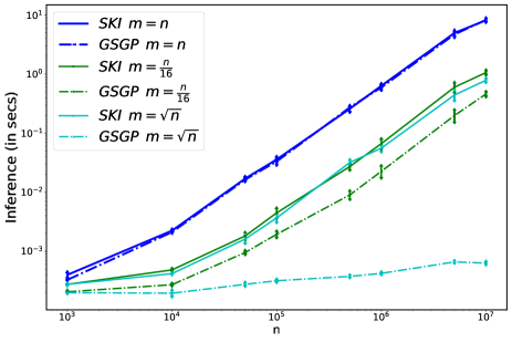
Figure 3: Per-iteration time taken by the SKI and GSGP methods on a synthetic dataset for posterior mean approximation. We see significant speedups when the grid size m𝑚m is relatively small compared to n𝑛n. Even when m𝑚m is larger, e.g., m=Θ(n)𝑚Θ𝑛m=\Theta(n), GSGP performs no worse than and sometimes improves upon SKI’s runtime, e.g., when m=n/16𝑚𝑛16m=n/16.

All linear solves use a tolerance of 0.01, and all kernels are squared exponential. We utilize cubic interpolation for all experiments and provide details on hardware and hyperparameters in Appendix C.1. In all cases, error bars show 95% confidence intervals of mean running time over independent trials.

Dataset n𝑛n d𝑑d m𝑚m Time Memory
Sound 59.3K 1 8K 0.433 0.247
59.3K 1 60K 0.941 0.505
Radar 10.5M 3 51.2K 0.014 0.007
10.5M 3 6.4M 0.584 0.425
Precipitation 528K 3 128K 0.326 0.366
528K 3 528K 0.491 0.628
528K 3 1.2M 0.806 2.941
Table 1: Ratios of GSGP to SKI per-iteration time and memory usage for posterior mean approximation for different values of m𝑚m and n𝑛n. GSGP shows large improvements in a range of settings, even with very large grid size m𝑚m.

Per-iteration resource usage. We first compare the per-iteration runtime for posterior mean calculation using CG and Factorized CG on synthetic data of varying sizes. The function f(x)𝑓𝑥f(x) is a sine wave with two periods in the interval [0,1]01[0,1]. Random x𝑥x locations are sampled in the interval and y=f(x)+ϵ𝑦𝑓𝑥italic-ϵy=f(x)+\epsilon with ϵ𝒩(0,0.25)similar-toitalic-ϵ𝒩00.25\epsilon\sim\mathcal{N}(0,0.25); grid points are equally spaced on [0,1]01[0,1]. Figure 3 shows the average per-iteration inference time over all iterations of 8 independent trials for increasing n𝑛n and three different settings of grid size: m=n𝑚𝑛m=n, m=n/16𝑚𝑛16m=n/16 and m=n𝑚𝑛m=\sqrt{n}. GSGP is substantially faster when m<n𝑚𝑛m<n (note log scale) and no slower when m=n𝑚𝑛m=n.

Memory usage is another important consideration. Table 1 compares both per-iteration running time and memory usage for posterior mean inference on our real data sets.

Per-iteration time is averaged over one run of CG and FCG for each setting; memory usage is calculated as 𝚗𝚗𝚣(W)+m+n𝚗𝚗𝚣𝑊𝑚𝑛\mathtt{nnz}(W)+m+n for SKI and 𝚗𝚗𝚣(WTW)+2m𝚗𝚗𝚣superscript𝑊𝑇𝑊2𝑚\mathtt{nnz}(W^{T}W)+2m for GSGP, where 𝚗𝚗𝚣(A)𝚗𝚗𝚣𝐴\mathtt{nnz}(A) is the number of nonzero entries of A𝐴A. The gains are significant, especially when mnmuch-less-than𝑚𝑛m\ll n, and gains in time and/or memory are possible even when m𝑚m equals or exceeds n𝑛n (e.g., precipitation, m{528K,1.2M}𝑚528K1.2Mm\in\{528\mathrm{K},1.2\mathrm{M}\}); for very large m𝑚m it is more resource efficient to run the original algorithm (or use FCG without precomputing WTWsuperscript𝑊𝑇𝑊W^{T}W).

Refer to caption
Refer to caption
Refer to caption
Refer to caption
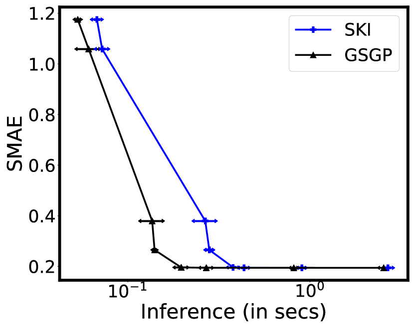
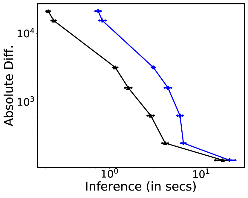
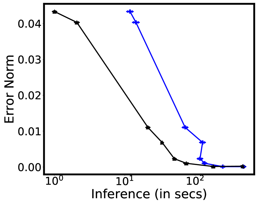
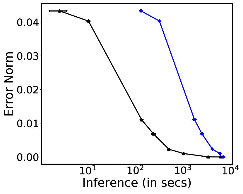
Figure 4: Error vs. runtime for approximate inference tasks on the sound dataset with varying grid size m𝑚m. GSGP gives much faster runtimes for fixed m𝑚m, allowing one to use a larger grid and achieve better runtime-accuracy tradeoffs than SKI. Times are averaged over 20 trials and include pre-processing. See text for description of error metrics.

Inference accuracy vs. time. A significant advantage of GSGP is the ability to realize speed-accuracy tradeoffs that were not previously possible. Figure 4 illustrates this for the sound data set (n=59.3K𝑛59.3Kn=59.3\mathrm{K}) by comparing error vs. running time for four different GP inference tasks for grid sizes m{1K,2K,5K,6K,8K,10K,30K,60K}𝑚1K2K5K6K8K10K30K60Km\in\{1\mathrm{K},2\mathrm{K},5\mathrm{K},6\mathrm{K},8\mathrm{K},10\mathrm{K},30\mathrm{K},60\mathrm{K}\}. For mean estimation we compute SMAE (mean absolute error normalized by the mean of observations) on a held-out test set of 691 points. For other tasks (log-likelihood, covariance) we compute error relative to a reference value computed with SKI for the highest m𝑚m using absolute difference for log-likelihood and Frobenius norm from the reference value for covariance matrices. For log-likelihood, we use 30 samples and tol=0.01𝑡𝑜𝑙0.01tol=0.01 for stochastic logdet approximation [5]. For covariance, we compute the 691×691691691691\times 691 posterior covariance matrix for test points, first using the exact SKI expressions (which requires 691 linear solves) and then using a rank-k𝑘k approximation [22], that, once computed, yields 𝒪(k)𝒪𝑘\mathcal{O}(k) time approximations of posterior covariances, for k=min{m,10000}𝑘𝑚10000k=\min\{m,10000\}. For each task, GSGP is faster when m<n𝑚𝑛m<n, sometimes substantially so, and achieves the same accuracy, leading to strictly better time-accuracy tradeoffs.
Refer to caption
Refer to caption
Refer to caption
Refer to caption
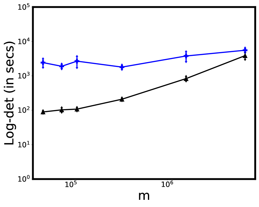
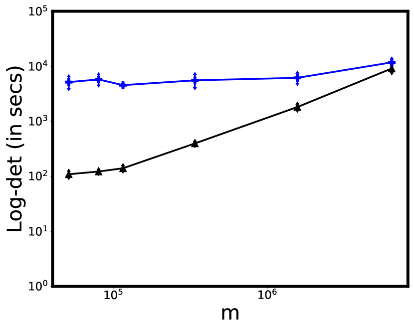
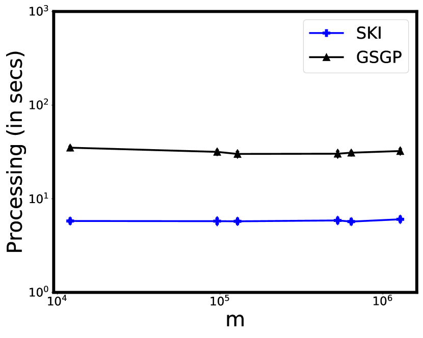
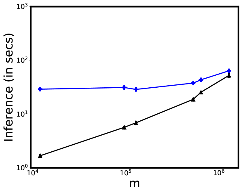
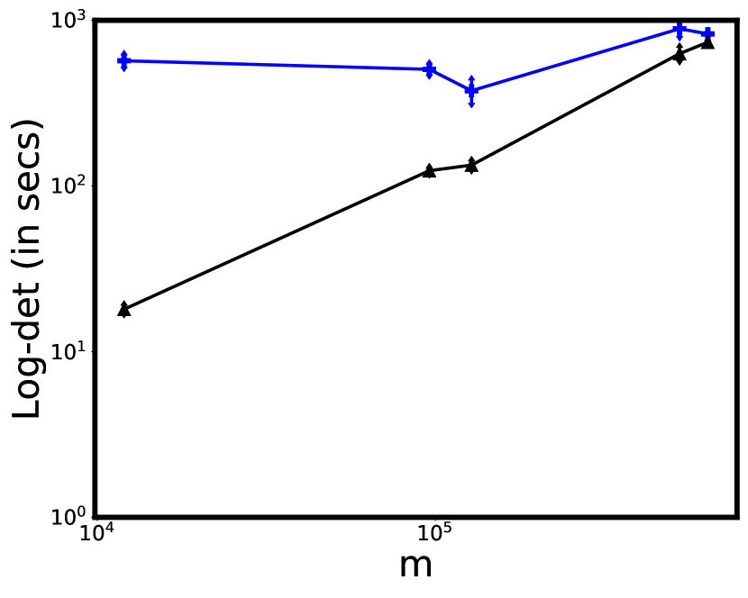
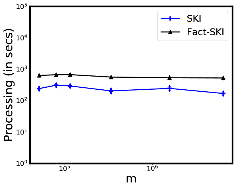
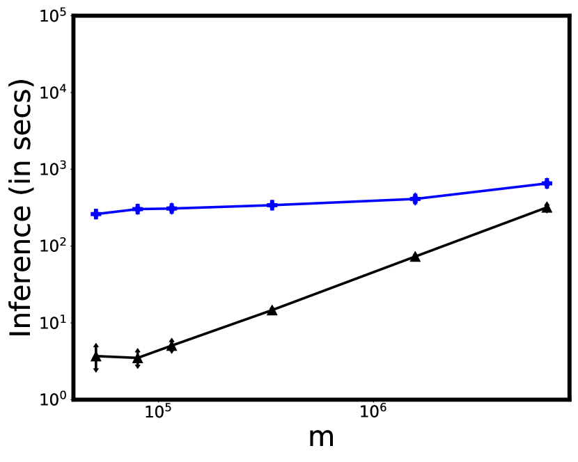
Figure 5: Runtime vs. grid size m𝑚m for GP inference tasks on the radar data set with 10.510.510.5M data points. We observe significantly faster runtimes for GSGP across all tasks and a wide range of grid sizes. From top to bottom: pre-processing time, mean inference runtime, and log-determinant runtime for tol=0.1𝑡𝑜𝑙0.1tol=0.1 and tol=0.01𝑡𝑜𝑙0.01tol=0.01 respectively. 30 random vectors are used in both log-determinant computations.

Very large n𝑛n. Figure 5 shows running time vs. m𝑚m for GP inference tasks on a data set of n=10.5M𝑛10.5Mn=10.5\mathrm{M} radar reflectivity measurements in three dimensions from 13 radar stations in the northeast US [1]. This is a situation where mnmuch-less-than𝑚𝑛m\ll n is highly relevant: even the smallest grid size of 51.2K=80×80×851.2K8080851.2\mathrm{K}=80\times 80\times 8 is of scientific value for summarizing broad-scale weather and biological activity. GSGP is much faster, e.g., roughly 150x and 15x faster for m=51.2K𝑚51.2𝐾m=51.2K on mean inference and log-likelihood estimation respectively after one-time pre-processing (first panel). Pre-processing is up to 3x slower for GSGP due to the need to compute WTWsuperscript𝑊𝑇𝑊W^{T}W. To perform only one mean inference, the overall time of GSGP and SKI including pre-processing is similar, which is consistent with the observation that typical solves use only tens of iterations, and some of the per-iteration gain is offset by pre-processing.

However, scientific modeling is highly iterative, and tasks other than mean inference perform many more iterations of linear solvers; the total time for GSGP in these cases is much smaller than SKI. In realistic applications with massive data sets, we expect WTWsuperscript𝑊𝑇𝑊W^{T}W to be computed once and saved to disk. GSGP also has the significant advantage that its memory footprint is 𝒪(m)𝒪𝑚\mathcal{O}(m), while SKI is 𝒪(m+n)𝒪𝑚𝑛\mathcal{O}(m+n). The data above is a subset from a national radar network, which was the limit on which SKI could run without exceeding 10GB of memory. To demonstrate scalability of GSGP, we ran on data from the entire national radar network with n=120M𝑛120𝑀n=120M for m=128K𝑚128𝐾m=128K, on which SKI far exceeds this memory limit. On this problem, GSGP takes 4861.604861.604861.60 +/- 233.42233.42233.42 seconds for pre-processing, and then 9.339.339.33 +/- 0.310.310.31 seconds for mean inference (averaged over 10 trials).

6 Conclusions and Future Work

Our work shows that the SKI method for approximate Gaussian process regression in fact performs exact inference for a natural grid-structured Gaussian process. We leverage this observation to give an implementation for the method with per-iteration complexity independent of the dataset size n𝑛n. This leads to significantly improved performance on a range of problems, including the ability to scale GP inference to radar datasets with over 100100100 million data points – a regime far beyond what can typically be handled by SKI or other approximation methods, such as inducing point and random feature approaches.

Our work leaves open a number of questions. Algorithmically, it would be interesting to explore if SKI can be efficiently implemented using direct, rather than iterative, solvers that take advantage of the Toeplitz and band-like structures of KGsubscript𝐾𝐺K_{G} and WTWsuperscript𝑊𝑇𝑊W^{T}W respectively. Theoretically, it would be interesting to further explore the grid-structured Gaussian process for which SKI performs exact inference. Intuitively, by interpolating data points to a grid, this method seems to suppress ‘high-frequency’ components of the kernel covariance function. Can this be analyzed to lead to formal approximation guarantees or practical guidance in how to choose the grid size?

References

  • [1] R. Angell and D. R. Sheldon. Inferring latent velocities from weather radar data using Gaussian processes. In Advances in Neural Information Processing Systems 31 (NeurIPS), pages 8984–8993, 2018.
  • [2] C. M. Bishop. Pattern Recognition and Machine Learning. Springer, 2006.
  • [3] Z. Cheng, M. Gadelha, S. Maji, and D. Sheldon. A bayesian perspective on the deep image prior. In Proceedings of the IEEE Conference on Computer Vision and Pattern Recognition (CVPR), pages 5443–5451, 2019.
  • [4] N. Cressie and G. Johannesson. Fixed rank kriging for very large spatial data sets. Journal of the Royal Statistical Society: Series B (Statistical Methodology), 70(1):209–226, 2008.
  • [5] K. Dong, D. Eriksson, H. Nickisch, D. Bindel, and A. G. Wilson. Scalable log determinants for Gaussian process kernel learning. In Advances in Neural Information Processing Systems 30 (NeurIPS), pages 6327–6337, 2017.
  • [6] J. R. Gardner, G. Pleiss, D. Bindel, K. Q. Weinberger, and A. G. Wilson. GPyTorch: Blackbox matrix-matrix Gaussian process inference with GPU acceleration. In Advances in Neural Information Processing Systems 31 (NeurIPS), pages 7576–7586, 2018.
  • [7] J. R. Gardner, G. Pleiss, R. Wu, K. Q. Weinberger, and A. G. Wilson. Product kernel interpolation for scalable Gaussian processes. In Proceedings of the \nth21 International Conference on Artificial Intelligence and Statistics (AISTATS), 2018.
  • [8] A. Garriga-Alonso, L. Aitchison, and C. E. Rasmussen. Deep Convolutional Networks as Shallow Gaussian Processes. International Conference on Learning Representations (ICLR), 2019.
  • [9] J. A. Gubner. Block matrix formulas, 2015. Accessed at: https://gubner.ece.wisc.edu/notes/BlockMatrixFormulas.pdf.
  • [10] J. Guinness and M. Fuentes. Circulant embedding of approximate covariances for inference from Gaussian data on large lattices. Journal of Computational and Graphical Statistics, 26(1):88–97, 2017.
  • [11] M. J. Heaton, A. Datta, A. O. Finley, R. Furrer, J. Guinness, R. Guhaniyogi, F. Gerber, R. B. Gramacy, D. Hammerling, M. Katzfuss, et al. A case study competition among methods for analyzing large spatial data. Journal of Agricultural, Biological and Environmental Statistics, 24(3):398–425, 2019.
  • [12] R. G. Keys. Cubic convolution interpolation for digital image processing. IEEE Transactions on Acoustics, Speech, and Signal Processing, 29(6):1153–1160, 1981.
  • [13] Q. Le, T. Sarlós, and A. Smola. Fastfood-approximating kernel expansions in loglinear time. In Proceedings of the \nth30 International Conference on Machine Learning (ICML), volume 85, 2013.
  • [14] D. Lee. Fast multiplication of a recursive block Toeplitz matrix by a vector and its application. Journal of Complexity, 2(4):295–305, 1986.
  • [15] J. Lee, Y. Bahri, R. Novak, S. Schoenholz, J. Pennington, and J. Sohl-Dickstein. Deep Neural Networks as Gaussian Processes. International Conference on Learning Representations (ICLR), 2018.
  • [16] G. Matheron. The Intrinsic Random Functions and Their Applications. Advances in Applied Probability, 5(3):439–468, 1973.
  • [17] A. G. d. G. Matthews, M. Rowland, J. Hron, R. E. Turner, and Z. Ghahramani. Gaussian process behaviour in wide deep neural networks. International Conference on Learning Representations (ICLR), 2018.
  • [18] G. Meanti, L. Carratino, L. Rosasco, and A. Rudi. Kernel methods through the roof: handling billions of points efficiently. arXiv:2006.10350, 2020.
  • [19] R. Neal. Lecture notes for sta 414: Statistical methods for machine learning and data mining, 2011. Accessed at: http://www.utstat.utoronto.ca/~radford/sta414.S11/week4a.pdf.
  • [20] R. M. Neal. Bayesian Learning for Neural Networks. PhD thesis, University of Toronto, 1995.
  • [21] R. Novak, L. Xiao, Y. Bahri, J. Lee, G. Yang, J. Hron, D. A. Abolafia, J. Pennington, and J. Sohl-Dickstein. Bayesian Deep Convolutional Networks with Many Channels are Gaussian Processes. In Proceedings of the \nth7 International Conference on Learning Representations (ICLR), 2019.
  • [22] G. Pleiss, J. R. Gardner, K. Q. Weinberger, and A. G. Wilson. Constant-time predictive distributions for Gaussian processes. In Proceedings of the \nth35 International Conference on Machine Learning (ICML), pages 4114–4123, 2018.
  • [23] J. Quiñonero-Candela and C. E. Rasmussen. A unifying view of sparse approximate Gaussian process regression. Journal of Machine Learning Research, 6(Dec):1939–1959, 2005.
  • [24] A. Rahimi and B. Recht. Random features for large-scale kernel machines. In Advances in Neural Information Processing Systems 20 (NeurIPS), pages 1177–1184, 2007.
  • [25] C. E. Rasmussen. Evaluation of Gaussian Processes and Other Methods for Non-linear Regression. University of Toronto, 1999.
  • [26] C. E. Rasmussen. Gaussian Processes in Machine Learning. In Advanced Lectures on Machine Learning, pages 63–71. Springer, 2004.
  • [27] Y. Saad and M. H. Schultz. GMRES: A generalized minimal residual algorithm for solving nonsymmetric linear systems. SIAM Journal on Scientific and Statistical Computing, 7(3):856–869, 1986.
  • [28] E. Snelson and Z. Ghahramani. Sparse Gaussian processes using pseudo-inputs. In Advances in Neural Information Processing Systems 18 (NeurIPS), pages 1257–1264, 2005.
  • [29] J. R. Stroud, M. L. Stein, and S. Lysen. Bayesian and maximum likelihood estimation for Gaussian processes on an incomplete lattice. Journal of computational and Graphical Statistics, 26(1):108–120, 2017.
  • [30] S. Ubaru, J. Chen, and Y. Saad. Fast estimation of tr(f(a))𝑡𝑟𝑓𝑎tr(f(a)) via stochastic Lanczos quadrature. Journal on Matrix Analysis and Applications, 38(4):1075–1099, 2017.
  • [31] C. Walder, K. I. Kim, and B. Schölkopf. Sparse multiscale Gaussian process regression. In Proceedings of the \nth25 International Conference on Machine Learning (ICML), pages 1112–1119, 2008.
  • [32] C. K. Williams. Computing with infinite networks. In Advances in Neural Information Processing Systems 10 (NeurIPS), pages 295–301, 1997.
  • [33] C. K. Williams and D. Barber. Bayesian Classification with Gaussian Processes. IEEE Transactions on Pattern Analysis and Machine Intelligence (PAMI), 20(12):1342–1351, 1998.
  • [34] C. K. Williams and M. Seeger. Using the Nyström method to speed up kernel machines. In Advances in Neural Information Processing Systems 14 (NeurIPS), pages 682–688, 2001.
  • [35] C. K. I. Williams and C. E. Rasmussen. Gaussian Processes for Regression. In Advances in Neural Information Processing Systems 9 (NeurIPS), pages 514–520, 1996.
  • [36] A. Wilson and R. Adams. Gaussian process kernels for pattern discovery and extrapolation. In Proceedings of the \nth30 International Conference on Machine Learning (ICML), pages 1067–1075, 2013.
  • [37] A. Wilson and H. Nickisch. Kernel interpolation for scalable structured Gaussian processes (KISS-GP). In Proceedings of the \nth32 International Conference on Machine Learning (ICML), pages 1775–1784, 2015.
  • [38] A. G. Wilson, C. Dann, and H. Nickisch. Thoughts on massively scalable gaussian processes. arXiv:1511.01870, 2015.

Supplementary Appendices

Appendix A Reformulation of SKI as Bayesian Linear Regression – Omitted Details

A.1 Equivalence between GSGP and SKI Approximation

Claim 1.

A GSGP with grid weights 𝛉𝛉\boldsymbol{\theta} drawn from a GP with covariance function k(𝐱,𝐱)𝑘𝐱superscript𝐱k(\mathbf{x},\mathbf{x}^{\prime}) is itself a GP with covariance function k~(𝐱,𝐱)=𝐰𝐱TKG𝐰𝐱~𝑘𝐱superscript𝐱superscriptsubscript𝐰𝐱𝑇subscript𝐾𝐺subscript𝐰superscript𝐱\tilde{k}(\mathbf{x},\mathbf{x}^{\prime})=\mathbf{w}_{\mathbf{x}}^{T}K_{G}\mathbf{w}_{\mathbf{x}^{\prime}}.

Proof.

For any finite number of input points 𝐱1,,𝐱nsubscript𝐱1subscript𝐱𝑛\mathbf{x}_{1},\ldots,\mathbf{x}_{n}, the joint distribution of (f(𝐱1),,f(𝐱n))𝑓subscript𝐱1𝑓subscript𝐱𝑛(f(\mathbf{x}_{1}),\ldots,f(\mathbf{x}_{n})) is zero-mean Gaussian, since each f(𝐱i)=𝐰𝐱iT𝜽𝑓subscript𝐱𝑖superscriptsubscript𝐰subscript𝐱𝑖𝑇𝜽f(\mathbf{x}_{i})=\mathbf{w}_{\mathbf{x}_{i}}^{T}\boldsymbol{\theta} is a linear transformation of the same zero-mean Gaussian random variable 𝜽𝜽\boldsymbol{\theta}. Therefore, f(𝐱)𝑓𝐱f(\mathbf{x}) is a zero-mean GP. For a particular pair of function values f(𝐱)𝑓𝐱f(\mathbf{x}) and f(𝐱)𝑓superscript𝐱f(\mathbf{x}^{\prime}), the covariance is given by

Cov(f(𝐱),f(𝐱))=Cov(𝐰𝐱T𝜽,𝐰𝐱T𝜽)=𝐰𝐱TCov(𝜽,𝜽)𝐰𝐱=𝐰𝐱TKG𝐰𝐱=k~(𝐱,𝐱).Cov𝑓𝐱𝑓superscript𝐱Covsuperscriptsubscript𝐰𝐱𝑇𝜽superscriptsubscript𝐰superscript𝐱𝑇𝜽superscriptsubscript𝐰𝐱𝑇Cov𝜽𝜽subscript𝐰superscript𝐱superscriptsubscript𝐰𝐱𝑇subscript𝐾𝐺subscript𝐰superscript𝐱~𝑘𝐱superscript𝐱\operatorname{Cov}(f(\mathbf{x}),f(\mathbf{x}^{\prime}))=\operatorname{Cov}(\mathbf{w}_{\mathbf{x}}^{T}\boldsymbol{\theta},\mathbf{w}_{\mathbf{x}^{\prime}}^{T}\boldsymbol{\theta})=\mathbf{w}_{\mathbf{x}}^{T}\operatorname{Cov}(\boldsymbol{\theta},\boldsymbol{\theta})\mathbf{w}_{\mathbf{x}^{\prime}}=\mathbf{w}_{\mathbf{x}}^{T}K_{G}\mathbf{w}_{\mathbf{x}^{\prime}}=\tilde{k}(\mathbf{x},\mathbf{x}^{\prime}). (3)

Therefore f𝑓f has the claimed covariance function. ∎

A.2 Exact Inference for GSGP

For completeness we derive the exact GSGP inference equations for Fact 2.

Proof of Fact 2.

GSGP is a standard linear basis function model and it is well known (see e.g., [19]) that the posterior mean and covariance of 𝜽𝜽\boldsymbol{\theta} given 𝐲𝐲\mathbf{y} are given by

𝔼[𝜽|𝐲]=1σ2[KG1+1σ2WTW]1WT𝐲.𝔼delimited-[]conditional𝜽𝐲1superscript𝜎2superscriptdelimited-[]superscriptsubscript𝐾𝐺11superscript𝜎2superscript𝑊𝑇𝑊1superscript𝑊𝑇𝐲\displaystyle\mathbb{E}[\boldsymbol{\theta}|\mathbf{y}]=\frac{1}{\sigma^{2}}\cdot\left[K_{G}^{-1}+\frac{1}{\sigma^{2}}W^{T}W\right]^{-1}\cdot W^{T}\mathbf{y}. (4)

and

Var(𝜽|𝐲)=[KG1+1σ2WTW]1.Varconditional𝜽𝐲superscriptdelimited-[]superscriptsubscript𝐾𝐺11superscript𝜎2superscript𝑊𝑇𝑊1\displaystyle\operatorname{Var}(\boldsymbol{\theta}|\mathbf{y})=\left[K_{G}^{-1}+\frac{1}{\sigma^{2}}W^{T}W\right]^{-1}. (5)

Using that for invertible A,B𝐴𝐵A,B, (AB)1=B1A1superscript𝐴𝐵1superscript𝐵1superscript𝐴1(AB)^{-1}=B^{-1}A^{-1} we can write:

1σ2[KG1+1σ2WTW]1=1σ2[I+1σ2KGWTW]1KG=(KGWTW+σ2I)1KG.1superscript𝜎2superscriptdelimited-[]superscriptsubscript𝐾𝐺11superscript𝜎2superscript𝑊𝑇𝑊11superscript𝜎2superscriptdelimited-[]𝐼1superscript𝜎2subscript𝐾𝐺superscript𝑊𝑇𝑊1subscript𝐾𝐺superscriptsubscript𝐾𝐺superscript𝑊𝑇𝑊superscript𝜎2𝐼1subscript𝐾𝐺\displaystyle\frac{1}{\sigma^{2}}\cdot\left[K_{G}^{-1}+\frac{1}{\sigma^{2}}W^{T}W\right]^{-1}=\frac{1}{\sigma^{2}}\cdot\left[I+\frac{1}{\sigma^{2}}K_{G}W^{T}W\right]^{-1}K_{G}=(K_{G}W^{T}W+\sigma^{2}I)^{-1}K_{G}.

Plugging back into the posterior mean equation (4) gives

𝔼[𝜽|𝐲]=(KGWTW+σ2I)1KGWT𝐲=𝐳¯.𝔼delimited-[]conditional𝜽𝐲superscriptsubscript𝐾𝐺superscript𝑊𝑇𝑊superscript𝜎2𝐼1subscript𝐾𝐺superscript𝑊𝑇𝐲¯𝐳\displaystyle\mathbb{E}[\boldsymbol{\theta}|\mathbf{y}]=(K_{G}W^{T}W+\sigma^{2}I)^{-1}K_{G}W^{T}\mathbf{y}=\mathbf{\bar{z}}.

By linearity since f(𝐱)=𝐰𝐱T𝜽𝑓𝐱superscriptsubscript𝐰𝐱𝑇𝜽f(\mathbf{x})=\mathbf{w}_{\mathbf{x}}^{T}\boldsymbol{\theta}, this gives the GSGP posterior mean equation, μf|𝒟(𝐱)=𝐰𝐱T𝐳¯subscript𝜇conditional𝑓𝒟𝐱superscriptsubscript𝐰𝐱𝑇¯𝐳\mu_{f|\mathcal{D}}(\mathbf{x})=\mathbf{w}_{\mathbf{x}}^{T}\mathbf{\bar{z}}. Similarly, plugging back into the posterior variance equation (5) gives:

Var(𝜽|𝐲)=σ2(KGWTW+σ2I)1KG=𝐂¯.Varconditional𝜽𝐲superscript𝜎2superscriptsubscript𝐾𝐺superscript𝑊𝑇𝑊superscript𝜎2𝐼1subscript𝐾𝐺¯𝐂\displaystyle\operatorname{Var}(\boldsymbol{\theta}|\mathbf{y})=\sigma^{2}(K_{G}W^{T}W+\sigma^{2}I)^{-1}K_{G}=\mathbf{\bar{C}}.

Again by linearity this gives the GSGP posterior variance equation kf|𝒟(𝐱,𝐱)=𝐰𝐱T𝐂¯𝐰𝐱subscript𝑘conditional𝑓𝒟𝐱superscript𝐱superscriptsubscript𝐰𝐱𝑇¯𝐂subscript𝐰superscript𝐱k_{f|\mathcal{D}}(\mathbf{x},\mathbf{x}^{\prime})=\mathbf{w}_{\mathbf{x}}^{T}\mathbf{\bar{C}}\mathbf{w}_{\mathbf{x^{\prime}}}.

Finally, it is well known [19] that the log likelihood of 𝐲𝐲\mathbf{y} under the GSGP linear basis function model is given by:

logPr(𝐲)=12[nlog(2π)+nlog(σ2)+logdetKGlogdet(𝐂¯)+1σ2𝐲T𝐲𝐳¯T𝐂¯1𝐳¯]Pr𝐲12delimited-[]𝑛2𝜋𝑛superscript𝜎2subscript𝐾𝐺¯𝐂1superscript𝜎2superscript𝐲𝑇𝐲superscript¯𝐳𝑇superscript¯𝐂1¯𝐳\displaystyle\log\Pr(\mathbf{y})=-\frac{1}{2}\left[n\log(2\pi)+n\log(\sigma^{2})+\log\det K_{G}-\log\det(\mathbf{\bar{C}})+\frac{1}{\sigma^{2}}\mathbf{y}^{T}\mathbf{y}-\mathbf{\bar{z}}^{T}\mathbf{\bar{C}}^{-1}\mathbf{\bar{z}}\right]

We can split logdet(𝐂¯)=logdet(σ2(KGWTW+σ2I)1KG)=mlogσ2logdet(KGWTW+σ2I)+logdet(KG)¯𝐂superscript𝜎2superscriptsubscript𝐾𝐺superscript𝑊𝑇𝑊superscript𝜎2𝐼1subscript𝐾𝐺𝑚superscript𝜎2subscript𝐾𝐺superscript𝑊𝑇𝑊superscript𝜎2𝐼subscript𝐾𝐺\log\det(\mathbf{\bar{C}})=\log\det(\sigma^{2}(K_{G}W^{T}W+\sigma^{2}I)^{-1}K_{G})=m\log\sigma^{2}-\log\det(K_{G}W^{T}W+\sigma^{2}I)+\log\det(K_{G}), and canceling this gives:

logPr(𝐲)=12[nlog(2π)+(nm)logσ2+logdet(KGWTW+σ2I)+1σ2𝐲T𝐲𝐳¯T𝐂¯1𝐳¯]Pr𝐲12delimited-[]𝑛2𝜋𝑛𝑚superscript𝜎2subscript𝐾𝐺superscript𝑊𝑇𝑊superscript𝜎2𝐼1superscript𝜎2superscript𝐲𝑇𝐲superscript¯𝐳𝑇superscript¯𝐂1¯𝐳\displaystyle\log\Pr(\mathbf{y})=-\frac{1}{2}\left[n\log(2\pi)+(n-m)\log\sigma^{2}+\log\det(K_{G}W^{T}W+\sigma^{2}I)+\frac{1}{\sigma^{2}}\mathbf{y}^{T}\mathbf{y}-\mathbf{\bar{z}}^{T}\mathbf{\bar{C}}^{-1}\mathbf{\bar{z}}\right] (6)

Additionally we can write:

𝐳¯T𝐂¯1𝐳¯superscript¯𝐳𝑇superscript¯𝐂1¯𝐳\displaystyle\mathbf{\bar{z}}^{T}\mathbf{\bar{C}}^{-1}\mathbf{\bar{z}} =1σ2𝐳¯TKG1(KGWTW+σ2I)(KGWTW+σ2I)1KGWT𝐲=1σ2𝐳¯TWT𝐲.absent1superscript𝜎2superscript¯𝐳𝑇superscriptsubscript𝐾𝐺1subscript𝐾𝐺superscript𝑊𝑇𝑊superscript𝜎2𝐼superscriptsubscript𝐾𝐺superscript𝑊𝑇𝑊superscript𝜎2𝐼1subscript𝐾𝐺superscript𝑊𝑇𝐲1superscript𝜎2superscript¯𝐳𝑇superscript𝑊𝑇𝐲\displaystyle=\frac{1}{\sigma^{2}}\mathbf{\bar{z}}^{T}K_{G}^{-1}(K_{G}W^{T}W+\sigma^{2}I)(K_{G}W^{T}W+\sigma^{2}I)^{-1}K_{G}W^{T}\mathbf{y}=\frac{1}{\sigma^{2}}\mathbf{\bar{z}}^{T}W^{T}\mathbf{y}.

Thus we have 1σ2𝐲T𝐲𝐳¯T𝐂¯1𝐳¯=𝐲T(𝐲W𝐳¯)σ21superscript𝜎2superscript𝐲𝑇𝐲superscript¯𝐳𝑇superscript¯𝐂1¯𝐳superscript𝐲𝑇𝐲𝑊¯𝐳superscript𝜎2\frac{1}{\sigma^{2}}\mathbf{y}^{T}\mathbf{y}-\mathbf{\bar{z}}^{T}\mathbf{\bar{C}}^{-1}\mathbf{\bar{z}}=\frac{\mathbf{y}^{T}(\mathbf{y}-W\mathbf{\bar{z}})}{\sigma^{2}}. Plugging back into (6) yields the log likelihood formula of Fact 2, completing the proof. ∎

A.3 Equivalence of GSGP Exact Inference and SKI

Theorem 1, which states that the GSGP and SKI inference equations are identical, follows directly from Claim 1, as GSGP is a Gaussian process whose kernel is exactly the approximate kernel used by SKI. For illustrative purposes, we also give a purely linear algebraic proof of Theorem 1 below:

Theorem 1.

The inference expressions of Fact 2 are identical to the SKI approximations of Def. 1.

Linear Algebraic Proof of Theorem 1.

The equivalence between the expressions for the posterior mean and posterior variance is a standard manipulation to convert between the “weight space” and “function space” view of a GP with an explicit feature expansion, e.g., Eqs. (2.11), (2.12) of [26]. We provide details with our notation for completeness. The correspondence between the two expressions for the log-likelihood is due to the same correspondence between “weight space” and “function space” views, though we are not aware of a specific reference that provides the formula in Fact 2.

First, recall these definitions from Def. 1 and Fact 2:

K~Xsubscript~𝐾𝑋\displaystyle\tilde{K}_{X} =WKGWTabsent𝑊subscript𝐾𝐺superscript𝑊𝑇\displaystyle=WK_{G}W^{T}
𝐳~~𝐳\displaystyle\mathbf{\tilde{z}} =(WKGWT+σ2I)1𝐲absentsuperscript𝑊subscript𝐾𝐺superscript𝑊𝑇superscript𝜎2𝐼1𝐲\displaystyle=\left(WK_{G}W^{T}+\sigma^{2}I\right)^{-1}\mathbf{y}
𝐳¯¯𝐳\displaystyle\mathbf{\bar{z}} =(KGWTW+σ2I)1KGWT𝐲absentsuperscriptsubscript𝐾𝐺superscript𝑊𝑇𝑊superscript𝜎2𝐼1subscript𝐾𝐺superscript𝑊𝑇𝐲\displaystyle=(K_{G}W^{T}W+\sigma^{2}I)^{-1}K_{G}W^{T}\mathbf{y}

Mean: The two mean expressions are 𝐰𝐱KGWT𝐳~subscript𝐰𝐱subscript𝐾𝐺superscript𝑊𝑇~𝐳\mathbf{w}_{\mathbf{x}}K_{G}W^{T}\mathbf{\tilde{z}} (Def. 1) and 𝐰𝐱𝐳¯subscript𝐰𝐱¯𝐳\mathbf{w}_{\mathbf{x}}\mathbf{\bar{z}} (Fact 2). Expanding these, it suffices to show that

KGWT(WKGWT+σ2I)1=(KGWTW+σ2I)1KGWT.subscript𝐾𝐺superscript𝑊𝑇superscript𝑊subscript𝐾𝐺superscript𝑊𝑇superscript𝜎2𝐼1superscriptsubscript𝐾𝐺superscript𝑊𝑇𝑊superscript𝜎2𝐼1subscript𝐾𝐺superscript𝑊𝑇\displaystyle K_{G}W^{T}\left(WK_{G}W^{T}+\sigma^{2}I\right)^{-1}=\left(K_{G}W^{T}W+\sigma^{2}I\right)^{-1}K_{G}W^{T}. (7)

This follows from the following claim:

Claim 5.

Let Am×n𝐴superscript𝑚𝑛A\in\mathbb{R}^{m\times n} and Bn×m𝐵superscript𝑛𝑚B\in\mathbb{R}^{n\times m}. Then

A(BA+σ2In)1=(AB+σ2Im)1A𝐴superscript𝐵𝐴superscript𝜎2subscript𝐼𝑛1superscript𝐴𝐵superscript𝜎2subscript𝐼𝑚1𝐴A(BA+\sigma^{2}I_{n})^{-1}=(AB+\sigma^{2}I_{m})^{-1}A

as long as BA+σ2In𝐵𝐴superscript𝜎2subscript𝐼𝑛BA+\sigma^{2}I_{n} and AB+σ2Im𝐴𝐵superscript𝜎2subscript𝐼𝑚AB+\sigma^{2}I_{m} are both invertible.

Proof.

Observe that (AB+σ2Im)A=A(BA+σ2In)=ABA+σ2A.𝐴𝐵superscript𝜎2subscript𝐼𝑚𝐴𝐴𝐵𝐴superscript𝜎2subscript𝐼𝑛𝐴𝐵𝐴superscript𝜎2𝐴(AB+\sigma^{2}I_{m})A=A(BA+\sigma^{2}I_{n})=ABA+\sigma^{2}A. If the matrices AB+σ2Im𝐴𝐵superscript𝜎2subscript𝐼𝑚AB+\sigma^{2}I_{m} and BA+σ2In𝐵𝐴superscript𝜎2subscript𝐼𝑛BA+\sigma^{2}I_{n} are invertible the result follows by left- and right-multiplying by the inverses. ∎

We obtain (7) from Claim 5, applied with A=KGWT𝐴subscript𝐾𝐺superscript𝑊𝑇A=K_{G}W^{T} and B=W𝐵𝑊B=W. As required by the claim, we have that both KGWTW+σ2Isubscript𝐾𝐺superscript𝑊𝑇𝑊superscript𝜎2𝐼K_{G}W^{T}W+\sigma^{2}I and WKGWT+σ2I𝑊subscript𝐾𝐺superscript𝑊𝑇superscript𝜎2𝐼WK_{G}W^{T}+\sigma^{2}I are invertible. For σ>0𝜎0\sigma>0, WKGWT+σ2I𝑊subscript𝐾𝐺superscript𝑊𝑇superscript𝜎2𝐼WK_{G}W^{T}+\sigma^{2}I is positive definite, which implies invertibility. KGWTWsubscript𝐾𝐺superscript𝑊𝑇𝑊K_{G}W^{T}W is similar to the positive semidefinite matrix KG1/2WTWKG1/2superscriptsubscript𝐾𝐺12superscript𝑊𝑇𝑊superscriptsubscript𝐾𝐺12K_{G}^{1/2}W^{T}WK_{G}^{1/2}, and thus has all non-negative eigenvalues. Thus, for σ>0𝜎0\sigma>0, KGWTW+σ2Isubscript𝐾𝐺superscript𝑊𝑇𝑊superscript𝜎2𝐼K_{G}W^{T}W+\sigma^{2}I has all positive eigenvalues (in particular, it has no zero eigenvalue) and so is invertible.

Covariance: The two expressions for covariance are 𝐰x𝐂~𝐰xsubscript𝐰𝑥~𝐂subscript𝐰𝑥\mathbf{w}_{x}\mathbf{\tilde{C}}\mathbf{w}_{x} (Def. 1) and 𝐰𝐱𝐂¯𝐰xsubscript𝐰𝐱¯𝐂subscript𝐰𝑥\mathbf{w}_{\mathbf{x}}\mathbf{\bar{C}}\mathbf{w}_{x} (Fact. 2) with

𝐂~~𝐂\displaystyle\mathbf{\tilde{C}} =KGKGWT(WKGWT+σ2I)1WKGabsentsubscript𝐾𝐺subscript𝐾𝐺superscript𝑊𝑇superscript𝑊subscript𝐾𝐺superscript𝑊𝑇superscript𝜎2𝐼1𝑊subscript𝐾𝐺\displaystyle=K_{G}-K_{G}W^{T}(WK_{G}W^{T}+\sigma^{2}I)^{-1}WK_{G}
𝐂¯¯𝐂\displaystyle\mathbf{\bar{C}} =σ2(KGWTW+σ2I)1KGabsentsuperscript𝜎2superscriptsubscript𝐾𝐺superscript𝑊𝑇𝑊superscript𝜎2𝐼1subscript𝐾𝐺\displaystyle=\sigma^{2}\left(K_{G}W^{T}W+\sigma^{2}I\right)^{-1}K_{G}

So it suffices to show that 𝐂~=𝐂¯~𝐂¯𝐂\mathbf{\tilde{C}}=\mathbf{\bar{C}}. Using Eq. 7, we have that

𝐂~=KG(KGWTW+σ2I)1KGWTWKG.~𝐂subscript𝐾𝐺superscriptsubscript𝐾𝐺superscript𝑊𝑇𝑊superscript𝜎2𝐼1subscript𝐾𝐺superscript𝑊𝑇𝑊subscript𝐾𝐺\mathbf{\tilde{C}}=K_{G}-(K_{G}W^{T}W+\sigma^{2}I)^{-1}K_{G}W^{T}WK_{G}.

Now, factor out KGsubscript𝐾𝐺K_{G} and simplify to get:

𝐂~~𝐂\displaystyle\mathbf{\tilde{C}} =[I(KGWTW+σ2I)1KGWTW]KGabsentdelimited-[]𝐼superscriptsubscript𝐾𝐺superscript𝑊𝑇𝑊superscript𝜎2𝐼1subscript𝐾𝐺superscript𝑊𝑇𝑊subscript𝐾𝐺\displaystyle=[I-(K_{G}W^{T}W+\sigma^{2}I)^{-1}K_{G}W^{T}W]K_{G}
=[(KGWTW+σ2I)1(KGWTW+σ2IKGWTW)]KGabsentdelimited-[]superscriptsubscript𝐾𝐺superscript𝑊𝑇𝑊superscript𝜎2𝐼1subscript𝐾𝐺superscript𝑊𝑇𝑊superscript𝜎2𝐼subscript𝐾𝐺superscript𝑊𝑇𝑊subscript𝐾𝐺\displaystyle=[(K_{G}W^{T}W+\sigma^{2}I)^{-1}\cdot(K_{G}W^{T}W+\sigma^{2}I-K_{G}W^{T}W)]K_{G}
=σ2(KGWTW+σ2I)1KG=𝐂¯absentsuperscript𝜎2superscriptsubscript𝐾𝐺superscript𝑊𝑇𝑊superscript𝜎2𝐼1subscript𝐾𝐺¯𝐂\displaystyle=\sigma^{2}(K_{G}W^{T}W+\sigma^{2}I)^{-1}K_{G}=\mathbf{\bar{C}}

Log likelihood: By matching terms in the two expressions and using the definition of K~Xsubscript~𝐾𝑋\tilde{K}_{X}, it suffices to show both of the following:

𝐲T𝐳~superscript𝐲𝑇~𝐳\displaystyle\mathbf{y}^{T}\mathbf{\tilde{z}} =𝐲T(𝐲W𝐳¯)σ2,absentsuperscript𝐲𝑇𝐲𝑊¯𝐳superscript𝜎2\displaystyle=\frac{\mathbf{y}^{T}(\mathbf{y}-W\mathbf{\bar{z}})}{\sigma^{2}}, (8)
logdet(WKGWT+σ2I)𝑊subscript𝐾𝐺superscript𝑊𝑇superscript𝜎2𝐼\displaystyle\log\det(WK_{G}W^{T}+\sigma^{2}I) =logdet(KGWTW+σ2I)+(nm)logσ2.absentsubscript𝐾𝐺superscript𝑊𝑇𝑊superscript𝜎2𝐼𝑛𝑚superscript𝜎2\displaystyle=\log\det(K_{G}W^{T}W+\sigma^{2}I)+(n-m)\log\sigma^{2}. (9)

For Eq. (8), we first observe that by our argument above that 𝐳¯=KGWT𝐳~¯𝐳subscript𝐾𝐺superscript𝑊𝑇~𝐳\mathbf{\bar{z}}=K_{G}W^{T}\mathbf{\tilde{z}}, we have

𝐲T(𝐲W𝐳¯)σ2=𝐲T(𝐲WKGWT𝐳~)σ2=𝐲T(IWKGWT(WKGWT+σ2I)1)𝐲σ2.superscript𝐲𝑇𝐲𝑊¯𝐳superscript𝜎2superscript𝐲𝑇𝐲𝑊subscript𝐾𝐺superscript𝑊𝑇~𝐳superscript𝜎2superscript𝐲𝑇𝐼𝑊subscript𝐾𝐺superscript𝑊𝑇superscript𝑊subscript𝐾𝐺superscript𝑊𝑇superscript𝜎2𝐼1𝐲superscript𝜎2\displaystyle\frac{\mathbf{y}^{T}(\mathbf{y}-W\mathbf{\bar{z}})}{\sigma^{2}}=\frac{\mathbf{y}^{T}(\mathbf{y}-WK_{G}W^{T}\mathbf{\tilde{z}})}{\sigma^{2}}=\frac{\mathbf{y}^{T}(I-WK_{G}W^{T}(WK_{G}W^{T}+\sigma^{2}I)^{-1})\mathbf{y}}{\sigma^{2}}. (10)

We have:

(IWKGWT(WKGWT+σ2I)1)𝐼𝑊subscript𝐾𝐺superscript𝑊𝑇superscript𝑊subscript𝐾𝐺superscript𝑊𝑇superscript𝜎2𝐼1\displaystyle(I-WK_{G}W^{T}(WK_{G}W^{T}+\sigma^{2}I)^{-1}) =[WKGWT+σ2IWKGWT](WKGWT+σ2I)1absentdelimited-[]𝑊subscript𝐾𝐺superscript𝑊𝑇superscript𝜎2𝐼𝑊subscript𝐾𝐺superscript𝑊𝑇superscript𝑊subscript𝐾𝐺superscript𝑊𝑇superscript𝜎2𝐼1\displaystyle=[WK_{G}W^{T}+\sigma^{2}I-WK_{G}W^{T}](WK_{G}W^{T}+\sigma^{2}I)^{-1}
=σ2(WKGWT+σ2I)1.absentsuperscript𝜎2superscript𝑊subscript𝐾𝐺superscript𝑊𝑇superscript𝜎2𝐼1\displaystyle=\sigma^{2}(WK_{G}W^{T}+\sigma^{2}I)^{-1}.

Thus we can simplify (10) to:

𝐲T(𝐲W𝐳¯)σ2=𝐲T(WKGWT+σ2I)1𝐲=𝐲T𝐳~.superscript𝐲𝑇𝐲𝑊¯𝐳superscript𝜎2superscript𝐲𝑇superscript𝑊subscript𝐾𝐺superscript𝑊𝑇superscript𝜎2𝐼1𝐲superscript𝐲𝑇~𝐳\displaystyle\frac{\mathbf{y}^{T}(\mathbf{y}-W\mathbf{\bar{z}})}{\sigma^{2}}=\mathbf{y}^{T}(WK_{G}W^{T}+\sigma^{2}I)^{-1}\mathbf{y}=\mathbf{y}^{T}\mathbf{\tilde{z}}. (11)

It remains to prove Eq. 9. This follows from the general claim:

Claim 6.

Let Am×n𝐴superscript𝑚𝑛A\in\mathbb{R}^{m\times n} and Bn×m𝐵superscript𝑛𝑚B\in\mathbb{R}^{n\times m}. Then:

det(BA+σ2In)=(σ2)nmdet(AB+σ2Im)𝐵𝐴superscript𝜎2subscript𝐼𝑛superscriptsuperscript𝜎2𝑛𝑚𝐴𝐵superscript𝜎2subscript𝐼𝑚\det(BA+\sigma^{2}I_{n})=(\sigma^{2})^{n-m}\det(AB+\sigma^{2}I_{m})
Proof.

The claim generalizes the Weinstein-Aronszajn identity, which states that det(BA+In)=det(AB+Im)𝐵𝐴subscript𝐼𝑛𝐴𝐵subscript𝐼𝑚\det(BA+I_{n})=\det(AB+I_{m}). It can be proven using the block determinant formulas in [9]. Let C=[σImABσIn].𝐶matrix𝜎subscript𝐼𝑚𝐴𝐵𝜎subscript𝐼𝑛C=\begin{bmatrix}\sigma I_{m}&-A\\ B&\sigma I_{n}\end{bmatrix}. We have:

det(C)=det(σIm)det(B(σIm)1A+σIn)𝐶𝜎subscript𝐼𝑚𝐵superscript𝜎subscript𝐼𝑚1𝐴𝜎subscript𝐼𝑛\displaystyle\det(C)=\det(\sigma I_{m})\cdot\det(B(\sigma I_{m})^{-1}A+\sigma I_{n}) =det(σIm)det(1σ(BA+σ2In))absent𝜎subscript𝐼𝑚1𝜎𝐵𝐴superscript𝜎2subscript𝐼𝑛\displaystyle=\det(\sigma I_{m})\cdot\det\left(\frac{1}{\sigma}(BA+\sigma^{2}I_{n})\right)
=det(σIm)det(1σIn)det(BA+σ2In)absent𝜎subscript𝐼𝑚1𝜎subscript𝐼𝑛𝐵𝐴superscript𝜎2subscript𝐼𝑛\displaystyle=\det(\sigma I_{m})\cdot\det\left(\frac{1}{\sigma}I_{n}\right)\cdot\det(BA+\sigma^{2}I_{n})

and similarly

det(C)=det(σIn)det(A(σIn)1B+σIm)𝐶𝜎subscript𝐼𝑛𝐴superscript𝜎subscript𝐼𝑛1𝐵𝜎subscript𝐼𝑚\displaystyle\det(C)=\det(\sigma I_{n})\cdot\det(A(\sigma I_{n})^{-1}B+\sigma I_{m}) =det(σIn)det(1σ(AB+σ2Im))absent𝜎subscript𝐼𝑛1𝜎𝐴𝐵superscript𝜎2subscript𝐼𝑚\displaystyle=\det(\sigma I_{n})\cdot\det\left(\frac{1}{\sigma}(AB+\sigma^{2}I_{m})\right)
=det(σIn)det(1σIm)det(AB+σ2Im).absent𝜎subscript𝐼𝑛1𝜎subscript𝐼𝑚𝐴𝐵superscript𝜎2subscript𝐼𝑚\displaystyle=\det(\sigma I_{n})\cdot\det\left(\frac{1}{\sigma}I_{m}\right)\cdot\det(AB+\sigma^{2}I_{m}).

Thus,

det(σIm)det(1σIn)det(BA+σ2In)𝜎subscript𝐼𝑚1𝜎subscript𝐼𝑛𝐵𝐴superscript𝜎2subscript𝐼𝑛\displaystyle\det(\sigma I_{m})\cdot\det\left(\frac{1}{\sigma}I_{n}\right)\cdot\det(BA+\sigma^{2}I_{n}) =det(σIn)det(1σIm)det(AB+σ2Im)absent𝜎subscript𝐼𝑛1𝜎subscript𝐼𝑚𝐴𝐵superscript𝜎2subscript𝐼𝑚\displaystyle=\det(\sigma I_{n})\cdot\det\left(\frac{1}{\sigma}I_{m}\right)\cdot\det(AB+\sigma^{2}I_{m})
det(BA+σ2In)𝐵𝐴superscript𝜎2subscript𝐼𝑛\displaystyle\det(BA+\sigma^{2}I_{n}) =σ2(nm)det(AB+σ2Im),absentsuperscript𝜎2𝑛𝑚𝐴𝐵superscript𝜎2subscript𝐼𝑚\displaystyle=\sigma^{2(n-m)}\cdot\det(AB+\sigma^{2}I_{m}),

giving the claim. ∎

Applying Claim 6 with A=KGWT𝐴subscript𝐾𝐺superscript𝑊𝑇A=K_{G}W^{T} and B=W𝐵𝑊B=W gives that det(W~KGWT+σ2I)=(σ2)nmdet(KGWTW+σ2I)~𝑊subscript𝐾𝐺superscript𝑊𝑇superscript𝜎2𝐼superscriptsuperscript𝜎2𝑛𝑚subscript𝐾𝐺superscript𝑊𝑇𝑊superscript𝜎2𝐼\det(\tilde{W}K_{G}W^{T}+\sigma^{2}I)=(\sigma^{2})^{n-m}\det(K_{G}W^{T}W+\sigma^{2}I) which in turn gives that logdet(WKGWT+σ2I)=logdet(KGWTW+σ2I)+(nm)logσ2𝑊subscript𝐾𝐺superscript𝑊𝑇superscript𝜎2𝐼subscript𝐾𝐺superscript𝑊𝑇𝑊superscript𝜎2𝐼𝑛𝑚superscript𝜎2\log\det(WK_{G}W^{T}+\sigma^{2}I)=\log\det(K_{G}W^{T}W+\sigma^{2}I)+(n-m)\log\sigma^{2} and so completes Eq. (9) and the theorem. ∎

A.4 Efficiency of Computing and Multiplying WTWsuperscript𝑊𝑇𝑊W^{T}W

Claim 2.

Assume that G={𝐠1,,𝐠m}𝐺subscript𝐠1subscript𝐠𝑚G=\{\mathbf{g}_{1},\ldots,\mathbf{g}_{m}\} has spacing s𝑠s, i.e., 𝐠i𝐠jssubscriptdelimited-∥∥subscript𝐠𝑖subscript𝐠𝑗𝑠\left\lVert\mathbf{g}_{i}-\mathbf{g}_{j}\right\rVert_{\infty}\geq s for any i,jm𝑖𝑗𝑚i,j\in m. Also assume that 𝐰𝐱jsubscriptsuperscript𝐰𝑗𝐱\mathbf{w}^{j}_{\mathbf{x}} is non-zero only if 𝐠j𝐱<rssubscriptnormsubscript𝐠𝑗𝐱𝑟𝑠\|\mathbf{g}_{j}-\mathbf{x}\|_{\infty}<r\cdot s for some fixed integer r𝑟r. Then WTWsuperscript𝑊𝑇𝑊W^{T}W can be computed in 𝒪(n(2r)2d)𝒪𝑛superscript2𝑟2𝑑\mathcal{O}(n(2r)^{2d}) time and has at most (4r1)dsuperscript4𝑟1𝑑(4r-1)^{d} entries per row. Therefore mv(WTW)=𝒪(m(4r1)d).𝑚𝑣superscript𝑊𝑇𝑊𝒪𝑚superscript4𝑟1𝑑mv(W^{T}W)=\mathcal{O}(m(4r-1)^{d}).

Proof.

First, write WTWsuperscript𝑊𝑇𝑊W^{T}W as a sum over data points:

WTW=i=1n𝐰𝐱i𝐰𝐱iT.superscript𝑊𝑇𝑊superscriptsubscript𝑖1𝑛subscript𝐰subscript𝐱𝑖superscriptsubscript𝐰subscript𝐱𝑖𝑇W^{T}W=\sum_{i=1}^{n}\mathbf{w}_{\mathbf{x}_{i}}\mathbf{w}_{\mathbf{x}_{i}}^{T}.

The vector 𝐰𝐱isubscript𝐰subscript𝐱𝑖\mathbf{w}_{\mathbf{x}_{i}} has nonzeros only for grid points 𝐠jsubscript𝐠𝑗\mathbf{g}_{j} such that 𝐠j𝐱irssubscriptnormsubscript𝐠𝑗subscript𝐱𝑖𝑟𝑠\|\mathbf{g}_{j}-\mathbf{x}_{i}\|_{\infty}\leq r\cdot s. Since the grid points have spacing s𝑠s, there are at most (2r)dsuperscript2𝑟𝑑(2r)^{d} such grid points. Therefore the outer product 𝐰𝐱i𝐰𝐱iTsubscript𝐰subscript𝐱𝑖superscriptsubscript𝐰subscript𝐱𝑖𝑇\mathbf{w}_{\mathbf{x}_{i}}\mathbf{w}_{\mathbf{x}_{i}}^{T} has at most (2r)2dsuperscript2𝑟2𝑑(2r)^{2d} non-zeros, and the sum can be computed in 𝒪(n(2r)2d)𝒪𝑛superscript2𝑟2𝑑\mathcal{O}(n(2r)^{2d}) time.

The sum is also sparse. The entry (WTW)jksubscriptsuperscript𝑊𝑇𝑊𝑗𝑘(W^{T}W)_{jk} is non-zero only if there is some data point 𝐱isubscript𝐱𝑖\mathbf{x}_{i} within distance r𝑟r from both 𝐠jsubscript𝐠𝑗\mathbf{g}_{j} and 𝐠ksubscript𝐠𝑘\mathbf{g}_{k} in each dimension. This is true only if 𝐠j𝐠k<2rssubscriptnormsubscript𝐠𝑗subscript𝐠𝑘2𝑟𝑠\|\mathbf{g}_{j}-\mathbf{g}_{k}\|_{\infty}<2r\cdot s. For a given grid point 𝐠jsubscript𝐠𝑗\mathbf{g}_{j}, there are at most (4r1)dsuperscript4𝑟1𝑑(4r-1)^{d} grid points 𝐠ksubscript𝐠𝑘\mathbf{g}_{k} satisfying 𝐠j𝐠k<2rssubscriptnormsubscript𝐠𝑗subscript𝐠𝑘2𝑟𝑠\|\mathbf{g}_{j}-\mathbf{g}_{k}\|_{\infty}<2r\cdot s (e.g., in 1 dimension there are 2r12𝑟12r-1 neighbors to the left, 2r12𝑟12r-1 neighbors to the right, plus the case k=j𝑘𝑗k=j). Therefore the j𝑗jth row of WTWsuperscript𝑊𝑇𝑊W^{T}W has as most (4r1)dsuperscript4𝑟1𝑑(4r-1)^{d} nonzeros, as claimed. ∎

A.5 Symmetric Reformulation of GSGP

Recall that directly replacing the SKI approximate inference equations of Definition 1 with the GSGP inference equations of Fact 2 reduces per-iteration cost from 𝒪(n+mlogm)𝒪𝑛𝑚𝑚\mathcal{O}(n+m\log m) to 𝒪(mlogm)𝒪𝑚𝑚\mathcal{O}(m\log m). However, the matrix KGWTW+σ2Isubscript𝐾𝐺superscript𝑊𝑇𝑊superscript𝜎2𝐼K_{G}W^{T}W+\sigma^{2}I is asymmetric, which prevents the application of symmetric system solvers like the conjugate gradient method with strong guarantees.

Here we describe a symmetric reformulation of GSGP that doesn’t compromise on per-iteration cost. We write the matrix (KGWTW+σ2I)1superscriptsubscript𝐾𝐺superscript𝑊𝑇𝑊superscript𝜎2𝐼1(K_{G}W^{T}W+\sigma^{2}I)^{-1}, whose application is required in both the posterior mean and covariance computation as:

(KGWTW+σ2I)1superscriptsubscript𝐾𝐺superscript𝑊𝑇𝑊superscript𝜎2𝐼1\displaystyle(K_{G}W^{T}W+\sigma^{2}I)^{-1} =(KGWTWKGKG1+σ2KGKG1)1absentsuperscriptsubscript𝐾𝐺superscript𝑊𝑇𝑊subscript𝐾𝐺superscriptsubscript𝐾𝐺1superscript𝜎2subscript𝐾𝐺superscriptsubscript𝐾𝐺11\displaystyle=(K_{G}W^{T}WK_{G}K_{G}^{-1}+\sigma^{2}K_{G}K_{G}^{-1})^{-1}
=KG(KGWTWKG+σ2KG)1.absentsubscript𝐾𝐺superscriptsubscript𝐾𝐺superscript𝑊𝑇𝑊subscript𝐾𝐺superscript𝜎2subscript𝐾𝐺1\displaystyle=K_{G}(K_{G}W^{T}WK_{G}+\sigma^{2}K_{G})^{-1}.

Applying the above matrix requires a symmetric solve in (KGWTWKG+σ2KG)1superscriptsubscript𝐾𝐺superscript𝑊𝑇𝑊subscript𝐾𝐺superscript𝜎2subscript𝐾𝐺1(K_{G}W^{T}WK_{G}+\sigma^{2}K_{G})^{-1}, along with a single 𝒪(mlogm)𝒪𝑚𝑚\mathcal{O}(m\log m) time MVM with KGsubscript𝐾𝐺K_{G}. Our per-iteration complexity thus remains at 𝒪(mlogm)𝒪𝑚𝑚\mathcal{O}(m\log m) – the matrix vector multiplication time for KGWTWKG+σ2KGsubscript𝐾𝐺superscript𝑊𝑇𝑊subscript𝐾𝐺superscript𝜎2subscript𝐾𝐺K_{G}W^{T}WK_{G}+\sigma^{2}K_{G}. However, this matrix is no longer of the ‘regularized form’ A+σ2I𝐴superscript𝜎2𝐼A+\sigma^{2}I, and may have worse condition number than WKGWT+σ2I𝑊subscript𝐾𝐺superscript𝑊𝑇superscript𝜎2𝐼WK_{G}W^{T}+\sigma^{2}I, possibly leading to slower convergence of iterative solvers like CG as compared to SKI.

We can similarly symmetrize the logdet computation in the likelihood expression by writing

logdet(KGWTW+σ2I)=logdet(KGWTWKG+σ2KG)logdet(KG).subscript𝐾𝐺superscript𝑊𝑇𝑊superscript𝜎2𝐼subscript𝐾𝐺superscript𝑊𝑇𝑊subscript𝐾𝐺superscript𝜎2subscript𝐾𝐺subscript𝐾𝐺\log\det(K_{G}W^{T}W+\sigma^{2}I)=\log\det(K_{G}W^{T}WK_{G}+\sigma^{2}K_{G})-\log\det(K_{G}).

Again however, it is unclear how this might affect the convergence of iterative methods for logdet approximation

Appendix B Factorized Iterative Methods – Omitted Details

B.1 Proofs for Factorized Update Steps

We give proofs of our fundamental factorized update steps described in Claims 3 and 4.

Claim 3.

For any 𝐳insubscript𝐳𝑖superscript𝑛\mathbf{z}_{i}\in\mathbb{R}^{n} with 𝐳i=W𝐳^i+ci𝐳0subscript𝐳𝑖𝑊subscript^𝐳𝑖subscript𝑐𝑖subscript𝐳0\mathbf{z}_{i}=W\mathbf{\hat{z}}_{i}+c_{i}\mathbf{z}_{0},

(WKGWT+σ2I)𝐳i=W𝐳^i+1+ci+1𝐳0,𝑊subscript𝐾𝐺superscript𝑊𝑇superscript𝜎2𝐼subscript𝐳𝑖𝑊subscript^𝐳𝑖1subscript𝑐𝑖1subscript𝐳0\displaystyle(WK_{G}W^{T}+\sigma^{2}I)\mathbf{z}_{i}=W\mathbf{\hat{z}}_{i+1}+c_{i+1}\mathbf{z}_{0},

where 𝐳^i+1=(KGWTW+σ2I)𝐳^i+ciKGWT𝐳0subscript^𝐳𝑖1subscript𝐾𝐺superscript𝑊𝑇𝑊superscript𝜎2𝐼subscript^𝐳𝑖subscript𝑐𝑖subscript𝐾𝐺superscript𝑊𝑇subscript𝐳0\mathbf{\hat{z}}_{i+1}=(K_{G}W^{T}W+\sigma^{2}I)\mathbf{\hat{z}}_{i}+c_{i}K_{G}W^{T}\mathbf{z}_{0} and ci+1=σ2cisubscript𝑐𝑖1superscript𝜎2subscript𝑐𝑖c_{i+1}=\sigma^{2}\cdot c_{i}. Call this operation a factorized update and denote it as (𝐳^i+1,ci+1)=𝒜(𝐳^i,ci)subscript^𝐳𝑖1subscript𝑐𝑖1𝒜subscript^𝐳𝑖subscript𝑐𝑖(\mathbf{\hat{z}}_{i+1},c_{i+1})=\mathcal{A}(\mathbf{\hat{z}}_{i},c_{i}). If the vector KGWT𝐳0subscript𝐾𝐺superscript𝑊𝑇subscript𝐳0K_{G}W^{T}\mathbf{z}_{0} is precomputed in 𝒪(n+mlogm)𝒪𝑛𝑚𝑚\mathcal{O}(n+m\log m) time, each subsequent factorized update takes 𝒪(mlogm)𝒪𝑚𝑚\mathcal{O}(m\log m) time.

Proof.

We have:

(WKGWT+σ2I)𝐳i𝑊subscript𝐾𝐺superscript𝑊𝑇superscript𝜎2𝐼subscript𝐳𝑖\displaystyle(WK_{G}W^{T}+\sigma^{2}I)\mathbf{z}_{i} =(WKGWT+σ2I)W𝐳^i+ci(WKGWT+σ2I)z0absent𝑊subscript𝐾𝐺superscript𝑊𝑇superscript𝜎2𝐼𝑊subscript^𝐳𝑖subscript𝑐𝑖𝑊subscript𝐾𝐺superscript𝑊𝑇superscript𝜎2𝐼subscript𝑧0\displaystyle=(WK_{G}W^{T}+\sigma^{2}I)W\mathbf{\hat{z}}_{i}+c_{i}(WK_{G}W^{T}+\sigma^{2}I)z_{0}
=W(KGWTW+σ2I)𝐳^i+ciW(KGWTz0)+ciσ2z0absent𝑊subscript𝐾𝐺superscript𝑊𝑇𝑊superscript𝜎2𝐼subscript^𝐳𝑖subscript𝑐𝑖𝑊subscript𝐾𝐺superscript𝑊𝑇subscript𝑧0subscript𝑐𝑖superscript𝜎2subscript𝑧0\displaystyle=W(K_{G}W^{T}W+\sigma^{2}I)\mathbf{\hat{z}}_{i}+c_{i}W(K_{G}W^{T}z_{0})+c_{i}\cdot\sigma^{2}\cdot z_{0}
=W[(KGWTW+σ2I)𝐳^i+ciKGWTz0]+ciσ2z0.absent𝑊delimited-[]subscript𝐾𝐺superscript𝑊𝑇𝑊superscript𝜎2𝐼subscript^𝐳𝑖subscript𝑐𝑖subscript𝐾𝐺superscript𝑊𝑇subscript𝑧0subscript𝑐𝑖superscript𝜎2subscript𝑧0\displaystyle=W\left[(K_{G}W^{T}W+\sigma^{2}I)\mathbf{\hat{z}}_{i}+c_{i}K_{G}W^{T}z_{0}\right]+c_{i}\cdot\sigma^{2}\cdot z_{0}.

which completes the derivation of the update.

As discussed in Sec. 3.1, it takes 𝒪(n+mlogm)𝒪𝑛𝑚𝑚\mathcal{O}(n+m\log m) time to precompute KGWT𝐳0subscript𝐾𝐺superscript𝑊𝑇subscript𝐳0K_{G}W^{T}\mathbf{z}_{0}, after which: it takes 𝒪(mlogm)𝒪𝑚𝑚\mathcal{O}(m\log m) time to compute (KGWTW+σ2I)𝐳^isubscript𝐾𝐺superscript𝑊𝑇𝑊superscript𝜎2𝐼subscript^𝐳𝑖(K_{G}W^{T}W+\sigma^{2}I)\mathbf{\hat{z}}_{i}, it takes 𝒪(m)𝒪𝑚\mathcal{O}(m) time to add in ciKGWT𝐳0subscript𝑐𝑖subscript𝐾𝐺superscript𝑊𝑇subscript𝐳0c_{i}K_{G}W^{T}\mathbf{z}_{0}, and it takes 𝒪(1)𝒪1\mathcal{O}(1) time to update cisubscript𝑐𝑖c_{i}, for a total of 𝒪(mlogm)𝒪𝑚𝑚\mathcal{O}(m\log m) time for each update.

Claim 4.

For any 𝐳i,𝐲insubscript𝐳𝑖subscript𝐲𝑖superscript𝑛\mathbf{z}_{i},\mathbf{y}_{i}\in\mathbb{R}^{n} with 𝐳i=W𝐳^i+ci𝐳0subscript𝐳𝑖𝑊subscript^𝐳𝑖subscript𝑐𝑖subscript𝐳0\mathbf{z}_{i}=W\mathbf{\hat{z}}_{i}+c_{i}\mathbf{z}_{0} and 𝐲i=W𝐲^i+di𝐲0subscript𝐲𝑖𝑊subscript^𝐲𝑖subscript𝑑𝑖subscript𝐲0\mathbf{y}_{i}=W\mathbf{\hat{y}}_{i}+d_{i}\mathbf{y}_{0},

𝐳iT𝐲i=𝐳^iTWTW𝐲^i+di𝐳^iTWT𝐲0+ci𝐲^iTWT𝐳0+cidi𝐲0T𝐳0.superscriptsubscript𝐳𝑖𝑇subscript𝐲𝑖superscriptsubscript^𝐳𝑖𝑇superscript𝑊𝑇𝑊subscript^𝐲𝑖subscript𝑑𝑖superscriptsubscript^𝐳𝑖𝑇superscript𝑊𝑇subscript𝐲0subscript𝑐𝑖superscriptsubscript^𝐲𝑖𝑇superscript𝑊𝑇subscript𝐳0subscript𝑐𝑖subscript𝑑𝑖superscriptsubscript𝐲0𝑇subscript𝐳0\displaystyle\mathbf{z}_{i}^{T}\mathbf{y}_{i}=\mathbf{\hat{z}}_{i}^{T}W^{T}W\mathbf{\hat{y}}_{i}+d_{i}\mathbf{\hat{z}}_{i}^{T}W^{T}\mathbf{y}_{0}+c_{i}\mathbf{\hat{y}}_{i}^{T}W^{T}\mathbf{z}_{0}+c_{i}d_{i}\mathbf{y}_{0}^{T}\mathbf{z}_{0}.

We denote the above operation by (𝐳^i,ci),(𝐲^i,di)subscript^𝐳𝑖subscript𝑐𝑖subscript^𝐲𝑖subscript𝑑𝑖\langle(\mathbf{\hat{z}}_{i},c_{i}),(\mathbf{\hat{y}}_{i},d_{i})\rangle.

Proof.

We have:

𝐳iT𝐲i=(W𝐳^i+ci𝐳0)T(W𝐲^i+di𝐲0)=𝐳^iTWTW𝐲^i+di𝐳^iTWT𝐲0+ci𝐲^iTWT𝐳0+cidi𝐲0T𝐳0,superscriptsubscript𝐳𝑖𝑇subscript𝐲𝑖superscript𝑊subscript^𝐳𝑖subscript𝑐𝑖subscript𝐳0𝑇𝑊subscript^𝐲𝑖subscript𝑑𝑖subscript𝐲0superscriptsubscript^𝐳𝑖𝑇superscript𝑊𝑇𝑊subscript^𝐲𝑖subscript𝑑𝑖superscriptsubscript^𝐳𝑖𝑇superscript𝑊𝑇subscript𝐲0subscript𝑐𝑖superscriptsubscript^𝐲𝑖𝑇superscript𝑊𝑇subscript𝐳0subscript𝑐𝑖subscript𝑑𝑖superscriptsubscript𝐲0𝑇subscript𝐳0\displaystyle\mathbf{z}_{i}^{T}\mathbf{y}_{i}=(W\mathbf{\hat{z}}_{i}+c_{i}\mathbf{z}_{0})^{T}(W\mathbf{\hat{y}}_{i}+d_{i}\mathbf{y}_{0})=\mathbf{\hat{z}}_{i}^{T}W^{T}W\mathbf{\hat{y}}_{i}+d_{i}\mathbf{\hat{z}}_{i}^{T}W^{T}\mathbf{y}_{0}+c_{i}\mathbf{\hat{y}}_{i}^{T}W^{T}\mathbf{z}_{0}+c_{i}d_{i}\mathbf{y}_{0}^{T}\mathbf{z}_{0},

giving the claim. ∎

Algorithm 3 Efficiently Factorized Conjugate Gradient (EFCG)
1:procedure EFCG(KG,W,𝐛,σ,𝐱0,ϵsubscript𝐾𝐺𝑊𝐛𝜎subscript𝐱0italic-ϵK_{G},W,\mathbf{b},\sigma,\mathbf{x}_{0},\epsilon)
2:     New Iterates:
3:               𝐯^k=[KGWTW+σ2I]𝐫^ksubscript^𝐯𝑘delimited-[]subscript𝐾𝐺superscript𝑊𝑇𝑊superscript𝜎2𝐼subscript^𝐫𝑘\mathbf{\hat{v}}_{k}=\left[K_{G}W^{T}W+\sigma^{2}I\right]\mathbf{\hat{r}}_{k},𝐮^k=WTW𝐫^ksubscript^𝐮𝑘superscript𝑊𝑇𝑊subscript^𝐫𝑘\mathbf{\hat{u}}_{k}=W^{T}W\mathbf{\hat{r}}_{k}
4:               𝐳^k=[KGWTW+σ2I]𝐩^ksubscript^𝐳𝑘delimited-[]subscript𝐾𝐺superscript𝑊𝑇𝑊superscript𝜎2𝐼subscript^𝐩𝑘\mathbf{\hat{z}}_{k}=\left[K_{G}W^{T}W+\sigma^{2}I\right]\mathbf{\hat{p}}_{k}, 𝐬^k=WTW𝐩^ksubscript^𝐬𝑘superscript𝑊𝑇𝑊subscript^𝐩𝑘\mathbf{\hat{s}}_{k}=W^{T}W\mathbf{\hat{p}}_{k}
5:     𝐫𝟎=𝐛K~𝐱0,𝐫^𝟎=𝟎,c0r=1formulae-sequencesubscript𝐫0𝐛~𝐾subscript𝐱0formulae-sequencesubscript^𝐫00superscriptsubscript𝑐0𝑟1\mathbf{r_{0}}=\mathbf{b}-\tilde{K}\mathbf{x}_{0},\,\mathbf{\hat{r}_{0}}=\mathbf{0},\,c_{0}^{r}=1
6:     𝐩^0=𝟎,c0p=1formulae-sequencesubscript^𝐩00superscriptsubscript𝑐0𝑝1\mathbf{\hat{p}}_{0}=\mathbf{0},\,c_{0}^{p}=1, 𝐱^0=𝟎,c0x=0formulae-sequencesubscript^𝐱00superscriptsubscript𝑐0𝑥0\,\mathbf{\hat{x}}_{0}=\mathbf{0},\,c_{0}^{x}=0
7:     𝐯^0=𝟎,𝐮^0=𝟎formulae-sequencesubscript^𝐯00subscript^𝐮00\mathbf{\hat{v}}_{0}=\mathbf{0},\mathbf{\hat{u}}_{0}=\mathbf{0}
8:     𝐳^0=𝟎,𝐬^0=𝟎formulae-sequencesubscript^𝐳00subscript^𝐬00\mathbf{\hat{z}}_{0}=\mathbf{0},\mathbf{\hat{s}}_{0}=\mathbf{0}
9:     for k=0𝑘0k=0 to maxiter do
10:         αk=𝐮^kT𝐫^k+ckrckr𝐫0+2cir(𝐫^iTWT𝐫0)𝐬^kT𝐳^k+ckzckp𝐫0+ckp(𝐳^kTWT𝐫0)+ckz(𝐫^kTWT𝐫0)subscript𝛼𝑘superscriptsubscript^𝐮𝑘𝑇subscript^𝐫𝑘superscriptsubscript𝑐𝑘𝑟superscriptsubscript𝑐𝑘𝑟delimited-∥∥subscript𝐫02superscriptsubscript𝑐𝑖𝑟superscriptsubscript^𝐫𝑖𝑇superscript𝑊𝑇subscript𝐫0superscriptsubscript^𝐬𝑘𝑇subscript^𝐳𝑘superscriptsubscript𝑐𝑘𝑧superscriptsubscript𝑐𝑘𝑝delimited-∥∥subscript𝐫0superscriptsubscript𝑐𝑘𝑝superscriptsubscript^𝐳𝑘𝑇superscript𝑊𝑇subscript𝐫0superscriptsubscript𝑐𝑘𝑧superscriptsubscript^𝐫𝑘𝑇superscript𝑊𝑇subscript𝐫0\alpha_{k}=\frac{\mathbf{\hat{u}}_{k}^{T}\mathbf{\hat{r}}_{k}+c_{k}^{r}c_{k}^{r}\left\lVert\mathbf{r}_{0}\right\rVert+2c_{i}^{r}(\mathbf{\hat{r}}_{i}^{T}W^{T}\mathbf{r}_{0})}{\mathbf{\hat{s}}_{k}^{T}\mathbf{\hat{z}}_{k}+c_{k}^{z}c_{k}^{p}\left\lVert\mathbf{r}_{0}\right\rVert+c_{k}^{p}(\mathbf{\hat{z}}_{k}^{T}W^{T}\mathbf{r}_{0})+c_{k}^{z}(\mathbf{\hat{r}}_{k}^{T}W^{T}\mathbf{r}_{0})}
11:         (𝐱^k+1,ck+1x)=(𝐱^k,ckx)+αk(𝐩^k,ckp)subscript^𝐱𝑘1superscriptsubscript𝑐𝑘1𝑥subscript^𝐱𝑘superscriptsubscript𝑐𝑘𝑥subscript𝛼𝑘subscript^𝐩𝑘superscriptsubscript𝑐𝑘𝑝(\mathbf{\hat{x}}_{k+1},c_{k+1}^{x})=(\mathbf{\hat{x}}_{k},c_{k}^{x})+\alpha_{k}\cdot(\mathbf{\hat{p}}_{k},c_{k}^{p})
12:         (𝐫^k+1,ck+1r)=(𝐫^k,ckr)αk(𝐳^k+ckp(KGWT𝐫0),σ2ckp)subscript^𝐫𝑘1superscriptsubscript𝑐𝑘1𝑟subscript^𝐫𝑘superscriptsubscript𝑐𝑘𝑟subscript𝛼𝑘subscript^𝐳𝑘superscriptsubscript𝑐𝑘𝑝subscript𝐾𝐺superscript𝑊𝑇subscript𝐫0superscript𝜎2superscriptsubscript𝑐𝑘𝑝(\mathbf{\hat{r}}_{k+1},c_{k+1}^{r})=(\mathbf{\hat{r}}_{k},c_{k}^{r})-\alpha_{k}\cdot(\mathbf{\hat{z}}_{k}+c_{k}^{p}\cdot(K_{G}W^{T}\mathbf{r}_{0}),\sigma^{2}c_{k}^{p})
13:         [𝐯^k+1,𝐮^k+1]=(𝐫^k+1)subscript^𝐯𝑘1subscript^𝐮𝑘1subscript^𝐫𝑘1[\mathbf{\hat{v}}_{k+1},\mathbf{\hat{u}}_{k+1}]=\mathcal{B}(\mathbf{\hat{r}}_{k+1})
14:         if 𝐮^k+1T𝐫^k+1+ck+1rck+1r𝐫0+2ck+1r(𝐫^k+1TWT𝐫0)ϵsuperscriptsubscript^𝐮𝑘1𝑇subscript^𝐫𝑘1superscriptsubscript𝑐𝑘1𝑟superscriptsubscript𝑐𝑘1𝑟delimited-∥∥subscript𝐫02superscriptsubscript𝑐𝑘1𝑟superscriptsubscript^𝐫𝑘1𝑇superscript𝑊𝑇subscript𝐫0italic-ϵ\mathbf{\hat{u}}_{k+1}^{T}\mathbf{\hat{r}}_{k+1}+c_{k+1}^{r}c_{k+1}^{r}\left\lVert\mathbf{r}_{0}\right\rVert+2c_{k+1}^{r}(\mathbf{\hat{r}}_{k+1}^{T}W^{T}\mathbf{r}_{0})\leq\epsilon exit loop
15:         βk=𝐮^k+1T𝐫^k+1+ck+1rck+1r+2ck+1r(𝐫^k+1TWT𝐫0)𝐮^kT𝐫^k+ckrckr𝐫0+2ckr(𝐫^kTWT𝐫0)subscript𝛽𝑘superscriptsubscript^𝐮𝑘1𝑇subscript^𝐫𝑘1superscriptsubscript𝑐𝑘1𝑟superscriptsubscript𝑐𝑘1𝑟2superscriptsubscript𝑐𝑘1𝑟superscriptsubscript^𝐫𝑘1𝑇superscript𝑊𝑇subscript𝐫0superscriptsubscript^𝐮𝑘𝑇subscript^𝐫𝑘superscriptsubscript𝑐𝑘𝑟superscriptsubscript𝑐𝑘𝑟subscriptdelimited-∥∥𝐫02superscriptsubscript𝑐𝑘𝑟superscriptsubscript^𝐫𝑘𝑇superscript𝑊𝑇subscript𝐫0\beta_{k}=\frac{\mathbf{\hat{u}}_{k+1}^{T}\mathbf{\hat{r}}_{k+1}+c_{k+1}^{r}c_{k+1}^{r}+2c_{k+1}^{r}(\mathbf{\hat{r}}_{k+1}^{T}W^{T}\mathbf{r}_{0})}{\mathbf{\hat{u}}_{k}^{T}\mathbf{\hat{r}}_{k}+c_{k}^{r}c_{k}^{r}\left\lVert\mathbf{r}\right\rVert_{0}+2c_{k}^{r}(\mathbf{\hat{r}}_{k}^{T}W^{T}\mathbf{r}_{0})}
16:         (𝐩^k+1,ck+1p)=(𝐫^k+1,ck+1r)+βk(𝐩^k,ckp)subscript^𝐩𝑘1superscriptsubscript𝑐𝑘1𝑝subscript^𝐫𝑘1superscriptsubscript𝑐𝑘1𝑟subscript𝛽𝑘subscript^𝐩𝑘superscriptsubscript𝑐𝑘𝑝(\mathbf{\hat{p}}_{k+1},c_{k+1}^{p})=(\mathbf{\hat{r}}_{k+1},c_{k+1}^{r})+\beta_{k}\cdot(\mathbf{\hat{p}}_{k},c_{k}^{p})
17:         𝐬^k+1=𝐮^k+1+βk𝐬^ksubscript^𝐬𝑘1subscript^𝐮𝑘1subscript𝛽𝑘subscript^𝐬𝑘\mathbf{\hat{s}}_{k+1}=\mathbf{\hat{u}}_{k+1}+\beta_{k}\cdot\mathbf{\hat{s}}_{k}
18:         𝐳^k+1=𝐯^k+1+βk𝐳^ksubscript^𝐳𝑘1subscript^𝐯𝑘1subscript𝛽𝑘subscript^𝐳𝑘\mathbf{\hat{z}}_{k+1}=\mathbf{\hat{v}}_{k+1}+\beta_{k}\cdot\mathbf{\hat{z}}_{k}      
19:     return 𝐱k+1=W𝐱^k+1+ck+1x𝐫0+𝐱0subscript𝐱𝑘1𝑊subscript^𝐱𝑘1superscriptsubscript𝑐𝑘1𝑥subscript𝐫0subscript𝐱0\mathbf{x}_{k+1}=W\mathbf{\hat{x}}_{k+1}+c_{k+1}^{x}\cdot\mathbf{r}_{0}+\mathbf{x}_{0}

B.2 Efficiently Factorized Conjugate Gradient Algorithms

We now present Efficiently factorized conjugate gradient (EFCG) (Algorithm 3), which improves on our basic Factorized CG algorithm (Algorithm 2) by avoiding any extra multiplication with W𝑊W and WTWsuperscript𝑊𝑇𝑊W^{T}W. The central idea of EFCG is to exploit the fact that each time we perform a matrix-vector multiplication with the GSGP operator KGWTW+σ2Isubscript𝐾𝐺superscript𝑊𝑇𝑊superscript𝜎2𝐼K_{G}W^{T}W+\sigma^{2}I, we also must perform one with WTWsuperscript𝑊𝑇𝑊W^{T}W. We can save the result of this multiplication to avoid repeated work. In particular, this lets us avoid extra MVM costs associated with WTWsuperscript𝑊𝑇𝑊W^{T}W present in factorized inner products steps of Algorithm 2. Similar to Algorithm 2, Algorithm 3 also maintains iterates CG (Algorithm 1) exactly in the same compressed form 𝐱k=W𝐱^k+ckx𝐫0+𝐱0subscript𝐱𝑘𝑊subscript^𝐱𝑘superscriptsubscript𝑐𝑘𝑥subscript𝐫0subscript𝐱0\mathbf{x}_{k}=W\mathbf{\hat{x}}_{k}+c_{k}^{x}\mathbf{r}_{0}+\mathbf{x}_{0}, 𝐫k=W𝐫^k+ckr𝐫0subscript𝐫𝑘𝑊subscript^𝐫𝑘superscriptsubscript𝑐𝑘𝑟subscript𝐫0\mathbf{r}_{k}=W\mathbf{\hat{r}}_{k}+c_{k}^{r}\mathbf{r}_{0}, and 𝐩k=W𝐩^k+ckp𝐫0subscript𝐩𝑘𝑊subscript^𝐩𝑘superscriptsubscript𝑐𝑘𝑝subscript𝐫0\mathbf{p}_{k}=W\mathbf{\hat{p}}_{k}+c_{k}^{p}\mathbf{r}_{0}.

We let [𝐯,𝐮]=(𝐱)𝐯𝐮𝐱[\mathbf{v},\mathbf{u}]=\mathcal{B}(\mathbf{x}) denote the operation that returns 𝐯=[KGWTW+σ2I]𝐱𝐯delimited-[]subscript𝐾𝐺superscript𝑊𝑇𝑊superscript𝜎2𝐼𝐱\mathbf{v}=\left[K_{G}W^{T}W+\sigma^{2}I\right]\mathbf{x} and 𝐮=WTW𝐱𝐮superscript𝑊𝑇𝑊𝐱\mathbf{u}=W^{T}W\mathbf{x}. Since 𝐮𝐮\mathbf{u} must be computed as in intermediate step in computing 𝐯𝐯\mathbf{v}, this operation has the same cost as a standard matrix-vector-multiplicaiton with [KGWTW+σ2I]delimited-[]subscript𝐾𝐺superscript𝑊𝑇𝑊superscript𝜎2𝐼\left[K_{G}W^{T}W+\sigma^{2}I\right]. Notice that Algorithm 3 performs just one (𝐱)𝐱\mathcal{B}(\mathbf{x}) operation per iteration, requiring a single matrix vector multiplication with each of KGsubscript𝐾𝐺K_{G} and WTWsuperscript𝑊𝑇𝑊W^{T}W per iteration. Both KGWT𝐫0subscript𝐾𝐺superscript𝑊𝑇subscript𝐫0K_{G}W^{T}\mathbf{r}_{0} and WT𝐫0superscript𝑊𝑇subscript𝐫0W^{T}\mathbf{r}_{0} are precomputed.

In addition to (𝐱)𝐱\mathcal{B}(\mathbf{x}) operation, the superior efficiency of the EFCG Algorithm 3 over CG and Factorized CG can mainly be attributed to following facts:

  • It uses four new iterates: 𝐯^k=[KGWTW+σ2I]𝐫^ksubscript^𝐯𝑘delimited-[]subscript𝐾𝐺superscript𝑊𝑇𝑊superscript𝜎2𝐼subscript^𝐫𝑘\mathbf{\hat{v}}_{k}=\left[K_{G}W^{T}W+\sigma^{2}I\right]\mathbf{\hat{r}}_{k}, 𝐮^k=WTW𝐫^ksubscript^𝐮𝑘superscript𝑊𝑇𝑊subscript^𝐫𝑘\mathbf{\hat{u}}_{k}=W^{T}W\mathbf{\hat{r}}_{k}, 𝐳^k=[KGWTW+σ2I]𝐩^ksubscript^𝐳𝑘delimited-[]subscript𝐾𝐺superscript𝑊𝑇𝑊superscript𝜎2𝐼subscript^𝐩𝑘\mathbf{\hat{z}}_{k}=\left[K_{G}W^{T}W+\sigma^{2}I\right]\mathbf{\hat{p}}_{k} and 𝐬^k=WTW𝐩^ksubscript^𝐬𝑘superscript𝑊𝑇𝑊subscript^𝐩𝑘\mathbf{\hat{s}}_{k}=W^{T}W\mathbf{\hat{p}}_{k}. Given these iterates all factorized inner products can be computed without any extra multiplication with WTWsuperscript𝑊𝑇𝑊W^{T}W.

  • In case, the initial solution 𝐱0=𝟎subscript𝐱00\mathbf{x}_{0}=\mathbf{0}, which is the most common choice in practice for CG, K~𝐱0~𝐾subscript𝐱0\tilde{K}\mathbf{x}_{0} multiplication can be avoided. Also, observe that in SKI mean and covariance approximation (Definition 1), we only need WT𝐱k+1superscript𝑊𝑇subscript𝐱𝑘1W^{T}\mathbf{x}_{k+1} which is equal to WTW𝐱^k+1+WT𝐫0+WT𝐱0superscript𝑊𝑇𝑊subscript^𝐱𝑘1superscript𝑊𝑇subscript𝐫0superscript𝑊𝑇subscript𝐱0W^{T}W\mathbf{\hat{x}}_{k+1}+W^{T}\mathbf{r}_{0}+W^{T}\mathbf{x}_{0}. Since, WT𝐫0superscript𝑊𝑇subscript𝐫0W^{T}\mathbf{r}_{0} is pre-computed and WT𝐱0=0superscript𝑊𝑇subscript𝐱00W^{T}\mathbf{x}_{0}=0, no extra multiplication with W𝑊W or WTWsuperscript𝑊𝑇𝑊W^{T}W is required other than computing KGWT𝐫0subscript𝐾𝐺superscript𝑊𝑇subscript𝐫0K_{G}W^{T}\mathbf{r}_{0} and WT𝐫0superscript𝑊𝑇subscript𝐫0W^{T}\mathbf{r}_{0}.

In Algorithm 4, we present a further simplified variant on EFCG for the case when initial residual 𝐫0subscript𝐫0\mathbf{r}_{0} is in the span of W𝑊W to directly compute WT𝐱k+1superscript𝑊𝑇subscript𝐱𝑘1W^{T}\mathbf{x}_{k+1} where 𝐱k+1subscript𝐱𝑘1\mathbf{x}_{k+1} is the final solution returned by the EFCG algorithm. Observe SKI mean and covariance expressions of SKI definition (i.e., Definition 1), we always need to post-process 𝐱k+1subscript𝐱𝑘1\mathbf{x}_{k+1} as WT𝐱k+1superscript𝑊𝑇subscript𝐱𝑘1W^{T}\mathbf{x}_{k+1} to estimate them. Unlike EFCG, simplified EFCG (i.e., Algorithm 4) maintains a compressed form for 𝐫ksubscript𝐫𝑘\mathbf{r}_{k} using 𝐫^ksubscript^𝐫𝑘\mathbf{\hat{r}}_{k} (as 𝐫k=W𝐫^ksubscript𝐫𝑘𝑊subscript^𝐫𝑘\mathbf{r}_{k}=W\mathbf{\hat{r}}_{k}) and doesn’t maintain 𝐩ksubscript𝐩𝑘\mathbf{p}_{k}. In addition to that, Algorithm 4 also maintains another iterate 𝐱^k+1dsubscriptsuperscript^𝐱𝑑𝑘1\mathbf{\hat{x}}^{d}_{k+1} such that WT𝐱k+1=𝐱^k+1d+WT𝐱0superscript𝑊𝑇subscript𝐱𝑘1subscriptsuperscript^𝐱𝑑𝑘1superscript𝑊𝑇subscript𝐱0W^{T}\mathbf{x}_{k+1}=\mathbf{\hat{x}}^{d}_{k+1}+W^{T}\mathbf{x}_{0}.

Algorithm 4 Simplified EFCG – Initial residual (i.e., 𝐫0subscript𝐫0\mathbf{r}_{0}) is in span of W𝑊W
1:procedure EFCG(KG,W,𝐫^0,σ,ϵsubscript𝐾𝐺𝑊subscript^𝐫0𝜎italic-ϵK_{G},W,\mathbf{\hat{r}}_{0},\sigma,\epsilon)
2:     New Iterates:
3:               𝐯^k=[KGWTW+σ2I]𝐫^ksubscript^𝐯𝑘delimited-[]subscript𝐾𝐺superscript𝑊𝑇𝑊superscript𝜎2𝐼subscript^𝐫𝑘\mathbf{\hat{v}}_{k}=\left[K_{G}W^{T}W+\sigma^{2}I\right]\mathbf{\hat{r}}_{k},𝐮^k=WTW𝐫^ksubscript^𝐮𝑘superscript𝑊𝑇𝑊subscript^𝐫𝑘\mathbf{\hat{u}}_{k}=W^{T}W\mathbf{\hat{r}}_{k}
4:               𝐳^k=[KGWTW+σ2I]𝐩^ksubscript^𝐳𝑘delimited-[]subscript𝐾𝐺superscript𝑊𝑇𝑊superscript𝜎2𝐼subscript^𝐩𝑘\mathbf{\hat{z}}_{k}=\left[K_{G}W^{T}W+\sigma^{2}I\right]\mathbf{\hat{p}}_{k}, 𝐬^k=WTW𝐩^ksubscript^𝐬𝑘superscript𝑊𝑇𝑊subscript^𝐩𝑘\mathbf{\hat{s}}_{k}=W^{T}W\mathbf{\hat{p}}_{k}
5:     𝐱^0d=𝟎subscriptsuperscript^𝐱𝑑00\mathbf{\hat{x}}^{d}_{0}=\mathbf{0}
6:     𝐯^0,𝐮^0=(𝐫^0)subscript^𝐯0subscript^𝐮0subscript^𝐫0\mathbf{\hat{v}}_{0},\mathbf{\hat{u}}_{0}=\mathcal{B}(\mathbf{\hat{r}}_{0})
7:     𝐳^0=𝐯^0,𝐬^0=𝐮^0formulae-sequencesubscript^𝐳0subscript^𝐯0subscript^𝐬0subscript^𝐮0\mathbf{\hat{z}}_{0}=\mathbf{\hat{v}}_{0},\mathbf{\hat{s}}_{0}=\mathbf{\hat{u}}_{0}
8:     for k=1𝑘1k=1 to maxiter𝑚𝑎𝑥𝑖𝑡𝑒𝑟maxiter do
9:         αk=𝐮^kT𝐫^k𝐬^kT𝐳^ksubscript𝛼𝑘superscriptsubscript^𝐮𝑘𝑇subscript^𝐫𝑘superscriptsubscript^𝐬𝑘𝑇subscript^𝐳𝑘\alpha_{k}={\frac{\mathbf{\hat{u}}_{k}^{T}\mathbf{\hat{r}}_{k}}{\mathbf{\hat{s}}_{k}^{T}\mathbf{\hat{z}}_{k}}}
10:         𝐱^k+1d=𝐱^kd+αk𝐬^ksubscriptsuperscript^𝐱𝑑𝑘1subscriptsuperscript^𝐱𝑑𝑘subscript𝛼𝑘subscript^𝐬𝑘\mathbf{\hat{x}}^{d}_{k+1}=\mathbf{\hat{x}}^{d}_{k}+\alpha_{k}\cdot\mathbf{\hat{s}}_{k}
11:         𝐫^k+1=𝐫^kαk𝐳^ksubscript^𝐫𝑘1subscript^𝐫𝑘subscript𝛼𝑘subscript^𝐳𝑘\mathbf{\hat{r}}_{k+1}=\mathbf{\hat{r}}_{k}-\alpha_{k}\cdot\mathbf{\hat{z}}_{k}
12:         𝐯^k+1,𝐮^k+1=(𝐫^k+1)subscript^𝐯𝑘1subscript^𝐮𝑘1subscript^𝐫𝑘1\mathbf{\hat{v}}_{k+1},\mathbf{\hat{u}}_{k+1}=\mathcal{B}(\mathbf{\hat{r}}_{k+1})
13:         if 𝐮^k+1T𝐫^k+1ϵsuperscriptsubscript^𝐮𝑘1𝑇subscript^𝐫𝑘1italic-ϵ\mathbf{\hat{u}}_{k+1}^{T}\mathbf{\hat{r}}_{k+1}\leq\epsilon exit loop
14:         βk=𝐮^k+1T𝐫^k+1𝐮^kT𝐫^ksubscript𝛽𝑘superscriptsubscript^𝐮𝑘1𝑇subscript^𝐫𝑘1superscriptsubscript^𝐮𝑘𝑇subscript^𝐫𝑘\beta_{k}=\frac{\mathbf{\hat{u}}_{k+1}^{T}\mathbf{\hat{r}}_{k+1}}{\mathbf{\hat{u}}_{k}^{T}\mathbf{\hat{r}}_{k}}
15:         𝐬^k+1=𝐮^k+1+βk𝐬^ksubscript^𝐬𝑘1subscript^𝐮𝑘1subscript𝛽𝑘subscript^𝐬𝑘\mathbf{\hat{s}}_{k+1}=\mathbf{\hat{u}}_{k+1}+\beta_{k}\cdot\mathbf{\hat{s}}_{k}
16:         𝐳^k+1=𝐯^k+1+βk𝐳^ksubscript^𝐳𝑘1subscript^𝐯𝑘1subscript𝛽𝑘subscript^𝐳𝑘\mathbf{\hat{z}}_{k+1}=\mathbf{\hat{v}}_{k+1}+\beta_{k}\cdot\mathbf{\hat{z}}_{k}      
17:     return 𝐱^k+1dsubscriptsuperscript^𝐱𝑑𝑘1\mathbf{\hat{x}}^{d}_{k+1}

The requirement of initial residual 𝐫0subscript𝐫0\mathbf{r}_{0} to be in the span of W𝑊W can be met in two ways. For example, for SKI posterior mean inference, we set 𝐱0=1σ2𝐲subscript𝐱01superscript𝜎2𝐲\mathbf{{x}}_{0}=\frac{1}{\sigma^{2}}\cdot\mathbf{y} implying 𝐫0=𝐲[WKGWT+σ2I]1σ2𝐲=1σ2WKGWT𝐲subscript𝐫0𝐲delimited-[]𝑊subscript𝐾𝐺superscript𝑊𝑇superscript𝜎2𝐼1superscript𝜎2𝐲1superscript𝜎2𝑊subscript𝐾𝐺superscript𝑊𝑇𝐲\mathbf{r}_{0}=\mathbf{y}-\left[WK_{G}W^{T}+\sigma^{2}I\right]\frac{1}{\sigma^{2}}\cdot\mathbf{y}=-\frac{1}{\sigma^{2}}\cdot WK_{G}W^{T}\mathbf{y}, which lies in the span of W𝑊W. Consequently, we initiate Algorithm 4 with 𝐫^0=1σ2KGWT𝐲m×1subscript^𝐫01superscript𝜎2subscript𝐾𝐺superscript𝑊𝑇𝐲superscript𝑚1\mathbf{\hat{r}}_{0}=-\frac{1}{\sigma^{2}}\cdot K_{G}W^{T}\mathbf{y}\in\mathbb{R}^{m\times 1} and following the invariance of simplified EFCG algorithm, compute transformed solutions as WT𝐱k+1=𝐱^k+1d+1σ2WTysuperscript𝑊𝑇subscript𝐱𝑘1subscriptsuperscript^𝐱𝑑𝑘11superscript𝜎2superscript𝑊𝑇𝑦W^{T}\mathbf{x}_{k+1}=\mathbf{\hat{x}}^{d}_{k+1}+\frac{1}{\sigma^{2}}\cdot W^{T}y. Notice that simplified EFCG (unlike EFCG) does not require pre-computations of terms KGWT𝐫0subscript𝐾𝐺superscript𝑊𝑇subscript𝐫0K_{G}W^{T}\mathbf{r}_{0} and WT𝐫0superscript𝑊𝑇subscript𝐫0W^{T}\mathbf{r}_{0}. In fact, simplified ECFG requires only only multiplication with WTsuperscript𝑊𝑇W^{T}, i.e., to obtain WTysuperscript𝑊𝑇𝑦W^{T}y which is sufficient for both, initialization of 𝐫0subscript𝐫0\mathbf{r}_{0} and the transformed final solution WT𝐱k+1superscript𝑊𝑇subscript𝐱𝑘1W^{T}\mathbf{x}_{k+1} (which is equal to WT(K~X+σ2I)1𝐲superscript𝑊𝑇superscriptsubscript~𝐾𝑋superscript𝜎2𝐼1𝐲W^{T}\left(\tilde{K}_{X}+\sigma^{2}I\right)^{-1}\mathbf{y}). Hence, simplified EFCG can compute SKI posterior mean using only sufficient statistics (WTWsuperscript𝑊𝑇𝑊W^{T}W and WT𝐲superscript𝑊𝑇𝐲W^{T}\mathbf{y}).

A second way to meet the requirement of the initial residual 𝐫0subscript𝐫0\mathbf{r}_{0} being in the span of W𝑊W, is by setting 𝐱0=𝟎subscript𝐱00\mathbf{{x}}_{0}=\mathbf{0} when 𝐲^^𝐲\mathbf{\hat{y}} is provided such that 𝐲=W𝐲^𝐲𝑊^𝐲\mathbf{y}=W\mathbf{\hat{y}}. This is the case, e.g., in posterior covariance approximation. The final transformed solution WT𝐱k+1superscript𝑊𝑇subscript𝐱𝑘1W^{T}\mathbf{x}_{k+1} in this setting reduces to 𝐱^k+1dsubscriptsuperscript^𝐱𝑑𝑘1\mathbf{\hat{x}}^{d}_{k+1}. Notice for this setting also, we need only WTWsuperscript𝑊𝑇𝑊W^{T}W and do not require the matrix W𝑊W.

Consquently, simplified EFCG can compute both SKI posterior mean and covariance function using onlythe sufficient statistics (WTWsuperscript𝑊𝑇𝑊W^{T}W and WT𝐲superscript𝑊𝑇𝐲W^{T}\mathbf{y}) and without even realizing W𝑊W matrix in memory.

B.3 Factorized Lanczos Algorithms

The Lanczos algorithm can be utilized to factorize a symmetric matrix An×n𝐴superscript𝑛𝑛A\in\mathbb{R}^{n\times n} as QTQT𝑄𝑇superscript𝑄𝑇QTQ^{T} such that Tn×n𝑇superscript𝑛𝑛T\in\mathbb{R}^{n\times n} is a symmetric tridiagonal matrix and Qn×n𝑄superscript𝑛𝑛Q\in\mathbb{R}^{n\times n} is orthonormal matrix. Previously, it has been used with k𝑘k iterations (i.e. Algorithm 5) to compute low-rank and fast approximations of SKI covariance matrix and log-likelihood of the data. For further details, we refer readers to [22, 5].

Algorithm 5 Lanczos Algorithm (LA)
1:procedure LA(KG,W,𝐛,σ,ksubscript𝐾𝐺𝑊𝐛𝜎𝑘K_{G},W,\mathbf{b},\sigma,k)
2:     𝐪0=𝟎,𝐪1=𝐛,β1=0formulae-sequencesubscript𝐪00formulae-sequencesubscript𝐪1𝐛subscript𝛽10\mathbf{q}_{0}=\mathbf{0},\mathbf{q}_{1}=\mathbf{b},\beta_{1}=0
3:     Q:,1=𝐪1subscript𝑄:1subscript𝐪1Q_{:,1}=\mathbf{q}_{1}
4:     for i=1𝑖1i=1 to k𝑘k do
5:         𝐪i+1=K~𝐪iβi𝐪i1subscript𝐪𝑖1~𝐾subscript𝐪𝑖subscript𝛽𝑖subscript𝐪𝑖1\mathbf{q}_{i+1}=\tilde{K}\mathbf{q}_{i}-\beta_{i}\cdot\mathbf{q}_{i-1}
6:         αi=𝐪iT𝐪i+1subscript𝛼𝑖superscriptsubscript𝐪𝑖𝑇subscript𝐪𝑖1\alpha_{i}=\mathbf{q}_{i}^{T}\mathbf{q}_{i+1}
7:         Ti,i=αisubscript𝑇𝑖𝑖subscript𝛼𝑖T_{i,i}=\alpha_{i}
8:         if i==ki==k then exit loop
9:         𝐪i+1=𝐪iαi𝐪isubscript𝐪𝑖1subscript𝐪𝑖subscript𝛼𝑖subscript𝐪𝑖\mathbf{q}_{i+1}=\mathbf{q}_{i}-\alpha_{i}\cdot\mathbf{q}_{i}
10:         𝐪i+1=𝐪i+1[Q:,1,,Q:,i]([Q:,1,,Q:,i]T𝐪i+1)subscript𝐪𝑖1subscript𝐪𝑖1subscript𝑄:1subscript𝑄:𝑖superscriptsubscript𝑄:1subscript𝑄:𝑖𝑇subscript𝐪𝑖1\mathbf{q}_{i+1}=\mathbf{q}_{i+1}-\left[Q_{:,1},...,Q_{:,i}\right]\left(\left[Q_{:,1},...,Q_{:,i}\right]^{T}\mathbf{q}_{i+1}\right)
11:         βi+1=𝐪i+1subscript𝛽𝑖1delimited-∥∥subscript𝐪𝑖1\beta_{i+1}=\left\lVert\mathbf{q}_{i+1}\right\rVert
12:         Ti,i+1=Ti,i+1=βi+1subscript𝑇𝑖𝑖1subscript𝑇𝑖𝑖1subscript𝛽𝑖1T_{i,i+1}=T_{i,i+1}=\beta_{i+1}
13:         𝐪i+1=1βi+1𝐪i+1subscript𝐪𝑖11subscript𝛽𝑖1subscript𝐪𝑖1\mathbf{q}_{i+1}=\frac{1}{\beta_{i+1}}\cdot\mathbf{q}_{i+1}
14:         Q:,i+1=𝐪i+1subscript𝑄:𝑖1subscript𝐪𝑖1Q_{:,i+1}=\mathbf{q}_{i+1}      
15:     return Q𝑄Q, T𝑇T
Algorithm 6 Factorized Lanczos Algorithm (FLA)
1:procedure FLA(KG,W,𝐛,σ,ksubscript𝐾𝐺𝑊𝐛𝜎𝑘K_{G},W,\mathbf{b},\sigma,k)
2:     𝐪^0=𝟎,c0q=0,𝐪^1=𝟎,c1q=1,β1=0formulae-sequencesubscript^𝐪00formulae-sequencesuperscriptsubscript𝑐0𝑞0formulae-sequencesubscript^𝐪10formulae-sequencesuperscriptsubscript𝑐1𝑞1subscript𝛽10\mathbf{\hat{q}}_{0}=\mathbf{0},c_{0}^{q}=0,\mathbf{\hat{q}}_{1}=\mathbf{0},c_{1}^{q}=1,\beta_{1}=0
3:     Q^:,1=𝐪^1,𝚲=𝟎k×1,𝐝=𝟎k×1formulae-sequenceformulae-sequencesubscript^𝑄:1subscript^𝐪1𝚲0superscript𝑘1𝐝0superscript𝑘1\hat{Q}_{:,1}=\mathbf{\hat{q}}_{1},\mathbf{\Lambda}=\mathbf{0}\in\mathbb{R}^{k\times 1},\mathbf{d}=\mathbf{0}\in\mathbb{R}^{k\times 1}
4:     for i=1𝑖1i=1 to k𝑘k do
5:         (𝐪^i+1,ci+1q)=(𝐪^i,ciq)βi𝒜(𝐪^i1,ci1q)subscript^𝐪𝑖1superscriptsubscript𝑐𝑖1𝑞subscript^𝐪𝑖superscriptsubscript𝑐𝑖𝑞subscript𝛽𝑖𝒜subscript^𝐪𝑖1superscriptsubscript𝑐𝑖1𝑞(\mathbf{\hat{q}}_{i+1},c_{i+1}^{q})=(\mathbf{\hat{q}}_{i},c_{i}^{q})-\beta_{i}\cdot\mathcal{A}(\mathbf{\hat{q}}_{i-1},c_{i-1}^{q})
6:         αi=(𝐪^i,ciq),(𝐪^i+1,ci+1q)subscript𝛼𝑖subscript^𝐪𝑖superscriptsubscript𝑐𝑖𝑞subscript^𝐪𝑖1superscriptsubscript𝑐𝑖1𝑞\alpha_{i}=\langle(\mathbf{\hat{q}}_{i},c_{i}^{q}),(\mathbf{\hat{q}}_{i+1},c_{i+1}^{q})\rangle
7:         Ti,i=αi;subscript𝑇𝑖𝑖subscript𝛼𝑖T_{i,i}=\alpha_{i};    𝐝i=ciqsubscript𝐝𝑖superscriptsubscript𝑐𝑖𝑞\mathbf{d}_{i}=c_{i}^{q}
8:         if i==ki==k then exit loop
9:         (𝐪^i+1,ci+1q)=(𝐪^i,ciq)αi(𝐪^i,ciq)subscript^𝐪𝑖1superscriptsubscript𝑐𝑖1𝑞subscript^𝐪𝑖superscriptsubscript𝑐𝑖𝑞subscript𝛼𝑖subscript^𝐪𝑖superscriptsubscript𝑐𝑖𝑞(\mathbf{\hat{q}}_{i+1},c_{i+1}^{q})=(\mathbf{\hat{q}}_{i},c_{i}^{q})-\alpha_{i}\cdot(\mathbf{\hat{q}}_{i},c_{i}^{q})
10:         𝚲j=(Q^:,j,cjq),(𝐪^i+1,ci+1q);subscript𝚲𝑗subscript^𝑄:𝑗superscriptsubscript𝑐𝑗𝑞subscript^𝐪𝑖1superscriptsubscript𝑐𝑖1𝑞\mathbf{\Lambda}_{j}=\langle(\hat{Q}_{:,j},c_{j}^{q}),(\mathbf{\hat{q}}_{i+1},c_{i+1}^{q})\rangle;    j{1,,i}for-all𝑗1𝑖\forall j\in\{1,...,i\}
11:         𝐪^i+1=𝐪^i+1Q^:,1:i𝚲1:i;subscript^𝐪𝑖1subscript^𝐪𝑖1subscript^𝑄::1𝑖subscript𝚲:1𝑖\mathbf{\hat{q}}_{i+1}=\mathbf{\hat{q}}_{i+1}-\hat{Q}_{:,1:i}\mathbf{\Lambda}_{1:i};    ci+1q=ci+1q𝐝1:iT𝚲1:isuperscriptsubscript𝑐𝑖1𝑞superscriptsubscript𝑐𝑖1𝑞superscriptsubscript𝐝:1𝑖𝑇subscript𝚲:1𝑖c_{i+1}^{q}=c_{i+1}^{q}-\mathbf{d}_{1:i}^{T}\mathbf{\Lambda}_{1:i}
12:         βi+1=(𝐪^i+1,ci+1q),(𝐪^i+1,ci+1q)subscript𝛽𝑖1subscript^𝐪𝑖1superscriptsubscript𝑐𝑖1𝑞subscript^𝐪𝑖1superscriptsubscript𝑐𝑖1𝑞\beta_{i+1}=\sqrt{\langle(\mathbf{\hat{q}}_{i+1},c_{i+1}^{q}),(\mathbf{\hat{q}}_{i+1},c_{i+1}^{q})\rangle}
13:         Ti,i+1=Ti,i+1=βi+1subscript𝑇𝑖𝑖1subscript𝑇𝑖𝑖1subscript𝛽𝑖1T_{i,i+1}=T_{i,i+1}=\beta_{i+1}
14:         𝐪^i+1=1βi+1𝐪^i+1;subscript^𝐪𝑖11subscript𝛽𝑖1subscript^𝐪𝑖1\mathbf{\hat{q}}_{i+1}=\frac{1}{\beta_{i+1}}\cdot\mathbf{\hat{q}}_{i+1};    ci+1q=ci+1qβi+1superscriptsubscript𝑐𝑖1𝑞superscriptsubscript𝑐𝑖1𝑞subscript𝛽𝑖1c_{i+1}^{q}=\frac{c_{i+1}^{q}}{\beta_{i+1}}
15:         Q^:,i+1=𝐪^i+1subscript^𝑄:𝑖1subscript^𝐪𝑖1\hat{Q}_{:,i+1}=\mathbf{\hat{q}}_{i+1}      
16:     return Q^^𝑄\hat{Q}, T𝑇T, 𝐝𝐝\mathbf{d}
Algorithm 7 Efficiently Factorized Lanczos algorithm (EFLA)
1:procedure EFLA(KG,W,𝐛,σ,ksubscript𝐾𝐺𝑊𝐛𝜎𝑘K_{G},W,\mathbf{b},\sigma,k)
2:     New Iterates:
3:               P^:,i=WTWQ^:,isubscript^𝑃:𝑖superscript𝑊𝑇𝑊subscript^𝑄:𝑖\hat{P}_{:,i}=W^{T}W\hat{Q}_{:,i} and 𝐬^i=[KGWTW+σI]𝐪^isubscript^𝐬𝑖delimited-[]subscript𝐾𝐺superscript𝑊𝑇𝑊𝜎𝐼subscript^𝐪𝑖\mathbf{\hat{s}}_{i}=\left[K_{G}W^{T}W+\sigma I\right]\mathbf{\hat{q}}_{i}
4:     𝐪^0=𝟎,c0q=0,𝐪^1=𝟎,c1q=1,β1=0formulae-sequencesubscript^𝐪00formulae-sequencesuperscriptsubscript𝑐0𝑞0formulae-sequencesubscript^𝐪10formulae-sequencesuperscriptsubscript𝑐1𝑞1subscript𝛽10\mathbf{\hat{q}}_{0}=\mathbf{0},c_{0}^{q}=0,\mathbf{\hat{q}}_{1}=\mathbf{0},c_{1}^{q}=1,\beta_{1}=0
5:     Q^:,1:k=[𝟎,,𝟎]m×k,P^:,1:k=[𝟎,,𝟎]m×kformulae-sequencesubscript^𝑄::1𝑘00superscript𝑚𝑘subscript^𝑃::1𝑘00superscript𝑚𝑘\hat{Q}_{:,1:k}=[\mathbf{0},...,\mathbf{0}]\in\mathbb{R}^{m\times k},\hat{P}_{:,1:k}=[\mathbf{0},...,\mathbf{0}]\in\mathbb{R}^{m\times k}
6:     Q^:,1=𝐪^1,𝚲=𝟎k×1,𝐬^i=𝟎m×1,𝐝=𝟎k×1formulae-sequenceformulae-sequencesubscript^𝑄:1subscript^𝐪1𝚲0superscript𝑘1subscript^𝐬𝑖0superscript𝑚1𝐝0superscript𝑘1\hat{Q}_{:,1}=\mathbf{\hat{q}}_{1},\mathbf{\Lambda}=\mathbf{0}\in\mathbb{R}^{k\times 1},\mathbf{\hat{s}}_{i}=\mathbf{0}\in\mathbb{R}^{m\times 1},\mathbf{d}=\mathbf{0}\in\mathbb{R}^{k\times 1}
7:     for i=1𝑖1i=1 to k𝑘k do
8:         𝐪^i+1=𝐬^i+ciqKGWT𝐛βi𝐪^i1subscript^𝐪𝑖1subscript^𝐬𝑖superscriptsubscript𝑐𝑖𝑞subscript𝐾𝐺superscript𝑊𝑇𝐛subscript𝛽𝑖subscript^𝐪𝑖1\mathbf{\hat{q}}_{i+1}=\mathbf{\hat{s}}_{i}+c_{i}^{q}\cdot K_{G}W^{T}\mathbf{b}-\beta_{i}\cdot\mathbf{\hat{q}}_{i-1}
9:         ci+1q=σ2ciqβici1qsuperscriptsubscript𝑐𝑖1𝑞superscript𝜎2superscriptsubscript𝑐𝑖𝑞subscript𝛽𝑖superscriptsubscript𝑐𝑖1𝑞c_{i+1}^{q}=\sigma^{2}c_{i}^{q}-\beta_{i}c_{i-1}^{q}
10:         αi=P^:,iT𝐪^i+1+ciqci+1q+(ciq𝐪^i+1+ci+1q𝐪^i)TWT𝐛subscript𝛼𝑖superscriptsubscript^𝑃:𝑖𝑇subscript^𝐪𝑖1superscriptsubscript𝑐𝑖𝑞superscriptsubscript𝑐𝑖1𝑞superscriptsuperscriptsubscript𝑐𝑖𝑞subscript^𝐪𝑖1superscriptsubscript𝑐𝑖1𝑞subscript^𝐪𝑖𝑇superscript𝑊𝑇𝐛\alpha_{i}=\hat{P}_{:,i}^{T}\mathbf{\hat{q}}_{i+1}+c_{i}^{q}c_{i+1}^{q}+\left(c_{i}^{q}\cdot\mathbf{\hat{q}}_{i+1}+c_{i+1}^{q}\cdot\mathbf{\hat{q}}_{i}\right)^{T}W^{T}\mathbf{b}
11:         Ti,i=αi;subscript𝑇𝑖𝑖subscript𝛼𝑖T_{i,i}=\alpha_{i};    𝐝i=cisubscript𝐝𝑖subscript𝑐𝑖\mathbf{d}_{i}=c_{i}
12:         if i==ki==k then exit loop
13:         (𝐪^i+1,ci+1q)=(𝐪^i,ciq)αi(𝐪^i,ciq)subscript^𝐪𝑖1superscriptsubscript𝑐𝑖1𝑞subscript^𝐪𝑖superscriptsubscript𝑐𝑖𝑞subscript𝛼𝑖subscript^𝐪𝑖superscriptsubscript𝑐𝑖𝑞(\mathbf{\hat{q}}_{i+1},c_{i+1}^{q})=(\mathbf{\hat{q}}_{i},c_{i}^{q})-\alpha_{i}\cdot(\mathbf{\hat{q}}_{i},c_{i}^{q})
14:         𝚲1:i=P^:,1:iT𝐪^i+1+(ci+1q+𝐪^i+1TWT𝐛)𝐜1:i+ci+1qQ^:,1:iTWT𝐛subscript𝚲:1𝑖superscriptsubscript^𝑃::1𝑖𝑇subscript^𝐪𝑖1superscriptsubscript𝑐𝑖1𝑞superscriptsubscript^𝐪𝑖1𝑇superscript𝑊𝑇𝐛subscript𝐜:1𝑖superscriptsubscript𝑐𝑖1𝑞superscriptsubscript^𝑄::1𝑖𝑇superscript𝑊𝑇𝐛\mathbf{\Lambda}_{1:i}=\hat{P}_{:,1:i}^{T}\mathbf{\hat{q}}_{i+1}+\left(c_{i+1}^{q}+\mathbf{\hat{q}}_{i+1}^{T}W^{T}\mathbf{b}\right)\cdot\mathbf{c}_{1:i}+c_{i+1}^{q}\cdot\hat{Q}_{:,1:i}^{T}W^{T}\mathbf{b}
15:         𝐪^i+1=𝐪^i+1Q^:,1:i𝚲1:i;subscript^𝐪𝑖1subscript^𝐪𝑖1subscript^𝑄::1𝑖subscript𝚲:1𝑖\mathbf{\hat{q}}_{i+1}=\mathbf{\hat{q}}_{i+1}-\hat{Q}_{:,1:i}\mathbf{\Lambda}_{1:i};    ci+1q=ci+1q𝐝1:iT𝚲1:isuperscriptsubscript𝑐𝑖1𝑞superscriptsubscript𝑐𝑖1𝑞superscriptsubscript𝐝:1𝑖𝑇subscript𝚲:1𝑖c_{i+1}^{q}=c_{i+1}^{q}-\mathbf{d}_{1:i}^{T}\mathbf{\Lambda}_{1:i}
16:         𝐬^i+1,P^:,i+1=(𝐪^i+1)subscript^𝐬𝑖1subscript^𝑃:𝑖1subscript^𝐪𝑖1\mathbf{\hat{s}}_{i+1},\hat{P}_{:,i+1}=\mathcal{B}(\mathbf{\hat{q}}_{i+1})
17:         βi+1=P^:,i+1T𝐪^i+1+ci+1qci+1q+2ci+1q𝐪^i+1TWT𝐛subscript𝛽𝑖1superscriptsubscript^𝑃:𝑖1𝑇subscript^𝐪𝑖1superscriptsubscript𝑐𝑖1𝑞superscriptsubscript𝑐𝑖1𝑞2superscriptsubscript𝑐𝑖1𝑞superscriptsubscript^𝐪𝑖1𝑇superscript𝑊𝑇𝐛\beta_{i+1}=\sqrt{\hat{P}_{:,i+1}^{T}\mathbf{\hat{q}}_{i+1}+c_{i+1}^{q}c_{i+1}^{q}+2c_{i+1}^{q}\mathbf{\hat{q}}_{i+1}^{T}W^{T}\mathbf{b}}
18:         Ti,i+1=Ti,i+1=βi+1subscript𝑇𝑖𝑖1subscript𝑇𝑖𝑖1subscript𝛽𝑖1T_{i,i+1}=T_{i,i+1}=\beta_{i+1}
19:         𝐪^i+1=1βi+1𝐪^i+1;subscript^𝐪𝑖11subscript𝛽𝑖1subscript^𝐪𝑖1\mathbf{\hat{q}}_{i+1}=\frac{1}{\beta_{i+1}}\cdot\mathbf{\hat{q}}_{i+1};    ci+1q=ci+1qβi+1superscriptsubscript𝑐𝑖1𝑞superscriptsubscript𝑐𝑖1𝑞subscript𝛽𝑖1c_{i+1}^{q}=\frac{c_{i+1}^{q}}{\beta_{i+1}}
20:         𝐬^i+1=1βi+1𝐬^i+1;subscript^𝐬𝑖11subscript𝛽𝑖1subscript^𝐬𝑖1\mathbf{\hat{s}}_{i+1}=\frac{1}{\beta_{i+1}}\cdot\mathbf{\hat{s}}_{i+1};    P^:,i+1=1βi+1P^:,i+1subscript^𝑃:𝑖11subscript𝛽𝑖1subscript^𝑃:𝑖1\hat{P}_{:,i+1}=\frac{1}{\beta_{i+1}}\cdot\hat{P}_{:,i+1}
21:         Q^:,i+1=𝐪^i+1subscript^𝑄:𝑖1subscript^𝐪𝑖1\hat{Q}_{:,i+1}=\mathbf{\hat{q}}_{i+1}      
22:     return Q^^𝑄\hat{Q}, T𝑇T, 𝐝𝐝\mathbf{d}

Similar to Factorized CG, we derive factorized Lanczos algorithm (FLA) using factorized inner products and matrix vector multiplication, as described in Algorithm 6. We maintain all iterates in m×1superscript𝑚1\mathbb{R}^{m\times 1} similar to Factorized CG, in particular, Q:,in×1subscript𝑄:𝑖superscript𝑛1{Q}_{:,i}\in\mathbb{R}^{n\times 1} vectors are maintained in compressed form such that Q:,i=WQ^:,i+di𝐛subscript𝑄:𝑖𝑊subscript^𝑄:𝑖subscript𝑑𝑖𝐛Q_{:,i}=W\hat{Q}_{:,i}+d_{i}\cdot\mathbf{b}. The Tk×k𝑇superscript𝑘𝑘T\in\mathbb{R}^{k\times k} matrix of Lanczos algorithm is retained as it is in FLA. Furthermore, in a manner similar to EFCG, we derive efficient factorized algorithm (EFLA) as shown in Algorithm 7. Specifically, EFLA relies on two new iterates: P^:,i=WTWQ^:,isubscript^𝑃:𝑖superscript𝑊𝑇𝑊subscript^𝑄:𝑖\hat{P}_{:,i}=W^{T}W\hat{Q}_{:,i} and 𝐬^i=[KGWTW+σI]𝐪^isubscript^𝐬𝑖delimited-[]subscript𝐾𝐺superscript𝑊𝑇𝑊𝜎𝐼subscript^𝐪𝑖\mathbf{\hat{s}}_{i}=\left[K_{G}W^{T}W+\sigma I\right]\mathbf{\hat{q}}_{i} and maintains iterates of Lanczos algorithm as Q:,i=WQ^:,i+di𝐛subscript𝑄:𝑖𝑊subscript^𝑄:𝑖subscript𝑑𝑖𝐛Q_{:,i}=W\hat{Q}_{:,i}+d_{i}\cdot\mathbf{b}, similar to FLA. Notice that EFLA only requires one (𝐱)𝐱\mathcal{B}(\mathbf{x}) operation per loop thereby avoiding any extra MVMs with W𝑊W and WTWsuperscript𝑊𝑇𝑊W^{T}W, except one time pre-computations of KGWT𝐛subscript𝐾𝐺superscript𝑊𝑇𝐛K_{G}W^{T}\mathbf{b} and WT𝐛superscript𝑊𝑇𝐛W^{T}\mathbf{b}.

Appendix C Experiments – Omitted Details and Additional Results

C.1 Hardware and hyper-parameters details

We run all of our experiments on Intel Xeon Gold 6240 CPU @ 2.60GHz with 10 GB of RAM. In all experimental settings, our kernels are squared exponential kernels wrapped within a scale kernel [37, 5]. Therefore, our hyper-parameters are σ𝜎\sigma, length-scales and output-scale as also presented in Table 2. Length-scales are specific to each dimension for multi-dimensional datasets. For sine and sound datasets, we have utilized GPytorch to optimize hyper-parameters. For precipitation and radar datasets, we have considered previously optimized parameters in [5] and in [1], respectively.

Dataset σ𝜎\sigma Length-scale Output-scale
Sine 0.074 0.312 1.439
Sound 0.009 10.895 0.002
Radar 50.000 [0.250, 0.250, 200] 3.500
Precipitation 3.990 [3.094, 2.030, 0.189] 2.786
Table 2: Hyper-parameters used for all datasets. Length-scale is of size d𝑑d of each dataset.

C.2 Results: Synthetic sine dataset

Figure 6 depicts the number of iteration and pre-processing time taken by GSGP and SKI for synthetic sine dataset wrt number of sample, for the setting on which Figure 3 reports the results. The number of iterations for GSGP and SKI are always close and possibly differ only due to finite precision.
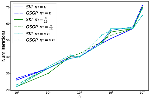
Refer to caption
Figure 6: Number of iterations taken by SKI and GSGP on synthetic dataset. Results are averaged over 8 trials.

C.3 Results: Precipitation dataset
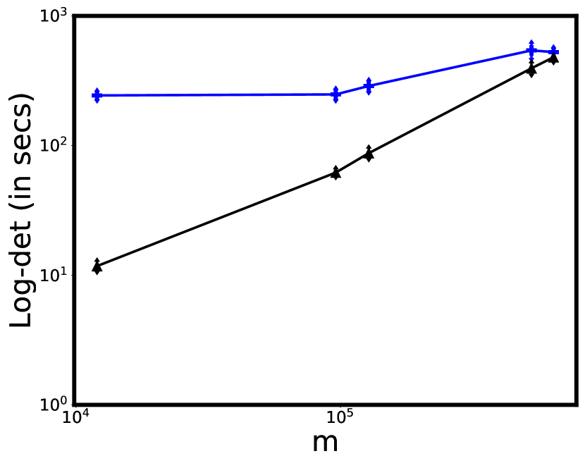
Refer to caption
Refer to caption
Refer to caption
Refer to caption
Figure 7: Inference time vs. m𝑚m for SKI inference tasks on precipitation data set. From left to right: pre-processing, mean inference, log-determinant for tol=0.1𝑡𝑜𝑙0.1tol=0.1 and for tol=0.01𝑡𝑜𝑙0.01tol=0.01 and using 30 random vectors.

Figure 7 shows running time vs. m𝑚m for GP inference tasks on precipitation data set of n=528K𝑛528Kn=528\mathrm{K} [5]. We consider m{12K,96K,128K,528K,640K}𝑚12K96K128K528K640Km\in\{12\mathrm{K},96\mathrm{K},128\mathrm{K},528\mathrm{K},640\mathrm{K}\}. This is a situation where even for m>n𝑚𝑛m>n, GSGP is faster compared to SKI. Pre-processing is up to 6x slower for GSGP due to the need to compute WTWsuperscript𝑊𝑇𝑊W^{T}W. To perform only one mean inference, the overall time of GSGP and SKI including pre-processing is similar as some of the per-iteration gains are offset by pre-processing. However, for the log-determinant computation task (as part of the log-likelihood computation), several more iterations of linear solvers are required as also demonstrated by log-det computation in Figure 7. It is worth noting that pre-processing of GSGP is required only once which can be performed initially for the log-det computation and later be utilized for the posterior mean and covariance inference. Therefore, overall, GSGP is more effective than SKI for all inference tasks.