Information contraction in noisy binary neural networks and its implications

Chuteng Zhou, Quntao Zhuang, Matthew Mattina, and Paul N. Whatmough C. Zhou is with the Arm ML Research Lab, Boston, MA USA (e-mail: chu.zhou@arm.com).Q. Zhuang is with the Department of Electrical and Computer Engineering and James C. Wyant College of Optical Sciences, University of Arizona, Tuscon, AZ USA (e-mail: zhuangquntao@email.arizona.edu).M. Mattina is with the Arm ML Research Lab, Boston, MA USA (e-mail: matthew.mattina@arm.com)P. N. Whatmough is with the Arm ML Research Lab, Boston, MA USA (e-mail: paul.whatmough@arm.com).
Abstract

Neural networks have gained importance as the machine learning models that achieve state-of-the-art performance on large-scale image classification, object detection and natural language processing tasks. In this paper, we consider noisy binary neural networks, where each neuron has a non-zero probability of producing an incorrect output. These noisy models may arise from biological, physical and electronic contexts and constitute an important class of models that are relevant to the physical world. Intuitively, the number of neurons in such systems has to grow to compensate for the noise while maintaining the same level of expressive power and computation reliability. Our key finding is a lower bound for the required number of neurons in noisy neural networks, which is first of its kind. To prove this lower bound, we take an information theoretic approach and obtain a novel strong data processing inequality (SDPI), which not only generalizes the Evans-Schulman results for binary symmetric channels to general channels, but also improves the tightness drastically when applied to estimate end-to-end information contraction in networks. Our SDPI can be applied to various information processing systems, including neural networks and cellular automata. Applying the SDPI in noisy binary neural networks, we obtain our key lower bound and investigate its implications on network depth-width trade-offs, our results suggest a depth-width trade-off for noisy neural networks that is very different from the established understanding regarding noiseless neural networks. Furthermore, we apply the SDPI to study fault-tolerant cellular automata and obtain bounds on the error correction overheads and the relaxation time. This paper offers new understanding of noisy information processing systems through the lens of information theory.

Index Terms:
Strong data processing inequality, noisy neural networks, depth-width trade-offs, fault tolerance, probabilistic cellular automata, relaxation time

I Introduction

Inspired by biological neural systems, artificial neural networks have gained great success in a wide variety of tasks such as computer vision, speech recognition and natural language processing. The majority of modern deep neural networks are based on artificial neurons which have a deterministic behavior. There has been rising interest in the study of neural networks with stochastic neurons. These noisy neural networks can be encountered in physical implementations of neural networks with analog components which are intrinsically noisy [1, 2, 3]. Studies of animal brains show that biological neurons are stochastic and our perception is fundamentally limited by the information that the brain can extract from the noisy dynamics of sensory neurons [4]. Furthermore, neurons that fire stochastically are used in models such as the restricted Boltzmann machines [5] and are shown to enhance the robustness in some deep neural networks [6]. Information theory provides a rigorous and insightful tool to model and understand noise in these systems.

Von Neumann [7] investigated the feasibility of computing Boolean functions with a circuit composed of noisy gates with a bounded number of inputs. He arrived at the conclusion that a Boolean function can be δ𝛿\delta-reliably (meaning the probability of producing a wrong answer for any input is at most δ𝛿\delta) computed at the cost of an increase in the circuit depth. Von Neumann’s results have been advanced over the years by a number of authors, notably Pippenger [8], Feder [9], Evans and Schulman [10]. The same question about noisy computation may be similarly posed for binary neural networks, which are known to be able to represent any Boolean functions [11]. In this paper, we leverage information theory to prove that, in analogy to Von Neumann’s result, an increasing number of neurons is the cost to pay for using noisy neurons to perform computation.

The analytic tool that is central to obtaining these results is the data processing inequality and its tighter variants. The data processing inequality (DPI) is a fundamental result of information theory. It formalizes the intuition that local data post-processing cannot increase mutual information. It is formulated as a contraction of mutual information for a Markov chain, which is I(X;Z)/I(X;Y)1𝐼𝑋𝑍𝐼𝑋𝑌1I(X;Z)/I(X;Y)\leq 1 for XYZ𝑋𝑌𝑍X\rightarrow Y\rightarrow Z. When the channel YZ𝑌𝑍Y\rightarrow Z can be characterized, channel dependent improvements of the DPI may be derived: I(X;Z)/I(X;Y)η𝐼𝑋𝑍𝐼𝑋𝑌𝜂I(X;Z)/I(X;Y)\leq\eta with η<1𝜂1\eta<1. These improved inequalities are called strong data processing inequalities (SDPIs) or sometimes quantified data processing inequalities.

The DPI and SDPIs are particularly useful for proving impossibility results and find applications in a wide range of fields such as physics [12], finance [13] and differential privacy [14]. Many of the results are obtained for Binary Symmetric Channels (BSCs), which is the most common scenario to consider. Regarding noisy computation, Pippenger [8] first derived an SDPI for BSCs and applied it to show an upper bound on the maximum tolerable component noise in Boolean formulas. Evans and Schulman [10] improved the SDPI bound of Pippenger and used it to obtain lower bounds on the complexity of reliable circuits with noisy components.

In this paper, we derive an SDPI for YZ𝑌𝑍Y\rightarrow Z being a multiple-input and multiple-output noisy channel. Our SDPI strictly improves the tightness of the end-to-end information contraction bound from the Evans and Schulman method [10]; more importantly, as our SDPI allows general channels other than BSCs being considered in Ref. [10], it can be applied to a wide range of different problems. As a first application, we apply this result to neural networks composed of noisy binary neurons. Our information contraction bound has a network width-depth trade-off relationship, which is then combined with network size complexity results to obtain lower bounds on the number of noisy neurons for reliable computation of Boolean functions such as the parity.

As a second application, we further apply our SDPI derived results to fault-tolerant cellular automata [15, 16, 17]. We obtain bounds on the error correction overhead and the relaxation time. These findings can potentially shed new light on a wide range of topics, including phase transitions in statistical physics [18, 19, 20] and stability of time-crystals [21].

The paper is organized as follows. In Section II, we introduce the basic definitions and notations. Section III contains the major theorem of our SDPI and its variants applicable to different scenarios. The application of our SDPI to noisy binary neural networks is presented in section IV, while the case to fault-tolerant cellular automata in Section V. Finally, we conclude in Section VI with a summary and some future directions.

II Definitions and notations

Without loss of generality, a noisy binary neuron considered in this paper is defined as follows. For a noisy binary neuron that has n𝑛n synapses (x1,,xn){0,1}nsubscript𝑥1subscript𝑥𝑛superscript01𝑛(x_{1},...,x_{n})\in\left\{0,1\right\}^{n} with the corresponding synaptic weights (w1,,wn)IRnsubscript𝑤1subscript𝑤𝑛IsuperscriptR𝑛(w_{1},...,w_{n})\in{\rm I\!R}^{n} and a bias θIR𝜃IR\theta\in{\rm I\!R}, the output of the neuron is a stochastic function

y^={ywithprobability 1p(1y)withprobabilityp,^𝑦cases𝑦withprobability1𝑝otherwise1𝑦withprobability𝑝otherwise\hat{y}\,=\,\begin{cases}y\;\;\mathrm{with\;probability\;}1-p\\ (1-y)\;\;\mathrm{with\;probability\;}p\end{cases}, (1)

where

y=sgn(i=1nwixi+θ).𝑦sgnsuperscriptsubscript𝑖1𝑛subscript𝑤𝑖subscript𝑥𝑖𝜃y\,=\,\mathrm{sgn}\left(\sum_{i=1}^{n}w_{i}x_{i}+\theta\right). (2)

And sgnsgn\mathrm{sgn} is the sign function defined as

sgn(α)={1ifα00Otherwise.sgn𝛼cases1if𝛼0otherwise0Otherwiseotherwise\mathrm{sgn}(\alpha)\,=\,\begin{cases}1\;\;\mathrm{if\;}\alpha\geq 0\\ 0\;\;\mathrm{Otherwise}\end{cases}. (3)

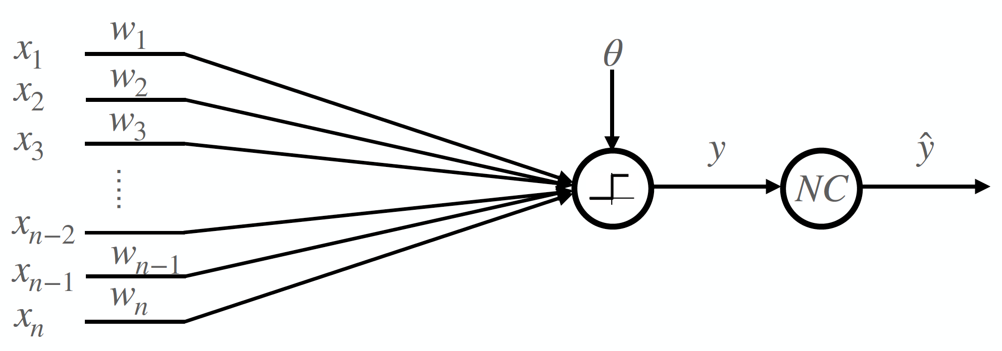
A schematic of this model is shown in Figure 1. A noisy binary neuron can be decomposed into a noiseless binary neuron followed by a noisy channel (denoted by NC in the schematic). With our definition above, the noisy channel is a BSC with bit flip probability p𝑝p (sometimes acronym-ed BSC(p)BSC𝑝\mathrm{BSC}(p)). A noisy binary neuron is said to be ξ𝜉\xi-noisy when the neuron misfiring probability p𝑝p is equal to ξ𝜉\xi. A noiseless binary neuron described above is also called a threshold gate in some literature and is a basic unit of the class Threshold Circuits (TC) in circuit complexity theory [22].
Refer to caption
Figure 1: Schematic of a noisy binary neuron with synapses (x1,,xn)subscript𝑥1subscript𝑥𝑛(x_{1},...,x_{n}), synaptic weights (w1,,wn)subscript𝑤1subscript𝑤𝑛(w_{1},...,w_{n}), bias θ𝜃\theta, binary step function activaition and noisy output y^^𝑦\hat{y}.

Even though so far we have only seen BSCs in our model, the key result of this paper is to prove an SDPI for a channel with an arbitrary number of input and output letter alphabets, which will then be used to improve bounds on estimating information contraction in a network composed of noisy binary neurons. Next, we give the definition of an n-input, m-output noisy channel XY𝑋𝑌X\rightarrow Y.

Definition 1.

An n-input, m-output noisy channel is a mapping between a categorical random variable on n𝑛n elements (or an n𝑛n-letter alphabet) X𝑋X and a categorical random variable on m𝑚m elements (or an m𝑚m-letter alphabet) Y𝑌Y. A noisy channel is characterized by its transition matrix 𝐀𝐀\mathbf{A} such that pY=pX𝐀subscript𝑝𝑌subscript𝑝𝑋𝐀p_{Y}=p_{X}\mathbf{A}, where pXsubscript𝑝𝑋p_{X} and pYsubscript𝑝𝑌p_{Y} are probability distributions over their letter alphabets represented as row vectors.

Following our definition, 𝐀𝐀\mathbf{A} is an n𝑛n by m𝑚m matrix whose (i,j)𝑖𝑗(i,j)-th entry ai,jsubscript𝑎𝑖𝑗a_{i,j} is the probability that input i𝑖i is transformed into output j𝑗j by the channel. The entries of A𝐴A are non-negative and the rows sum to 111: ai,j0subscript𝑎𝑖𝑗0a_{i,j}\geq 0 and jai,j=1subscript𝑗subscript𝑎𝑖𝑗1\sum_{j}a_{i,j}=1.

We hereby give the definition of a simply layered network, which is a constraint on neuron connectivity that we use throughout this paper.

Definition 2.

A neural network is said to be simply layered if its inputs and neurons can be partitioned into subsets called layers, such that every synaptic connection happens between adjacent layers and inputs only appear at layer 00.

The above definition describes the most commonly studied neural network architectures in a theoretical setting, namely the regular feed-forward networks with hidden layers but no skip connections allowed between non-adjacent layers.

Our main result will be concerning the mutual information

I(X;Y)=H(X)+H(Y)H(X,Y)=H(Y)H(Y|X)𝐼𝑋𝑌𝐻𝑋𝐻𝑌𝐻𝑋𝑌𝐻𝑌𝐻conditional𝑌𝑋I(X;Y)=H(X)+H(Y)-H(X,Y)=H(Y)-H(Y|X)

between two random variables X𝑋X and Y𝑌Y, where the Shannon entropy H(X)=xpX(x)log(pX(x))𝐻𝑋subscript𝑥subscript𝑝𝑋𝑥subscript𝑝𝑋𝑥H(X)=-\sum_{x}p_{X}(x)\log\left(p_{X}(x)\right) can be calculated from the probability distribution pXsubscript𝑝𝑋p_{X}. We use the natural logarithm in this paper, however, our results will not depend on this choice. Here

H(Y|X)=H(X,Y)H(X)=xpX(x)H(Y|X=x)𝐻conditional𝑌𝑋𝐻𝑋𝑌𝐻𝑋subscript𝑥subscript𝑝𝑋𝑥𝐻conditional𝑌𝑋𝑥H(Y|X)=H(X,Y)-H(X)=\sum_{x}p_{X}(x)H(Y|X=x)

is the conditional entropy, which can be calculated from the conditional probability pY|X=x()subscript𝑝conditional𝑌𝑋𝑥p_{Y|X=x}(\cdot).

III A Strong Data Processing Inequality for general n𝑛n-input m𝑚m-output noisy channels

In this section, we prove our SDPI of Theorem 1 and apply it to a network layer composed of noisy binary neurons, with Proposition 1 for independent noise and Proposition 2 for weakly-correlated noise.

Consider a Markov chain XYZ𝑋𝑌𝑍X\rightarrow Y\rightarrow Z, our objective is to bound the mutual information contraction ratio I(X;Z)/I(X;Y)𝐼𝑋𝑍𝐼𝑋𝑌I(X;Z)/I(X;Y) for YZ𝑌𝑍Y\rightarrow Z being an n𝑛n-input, m𝑚m-output noisy channel defined in Definition 1, as a function of the characteristics of YZ𝑌𝑍Y\rightarrow Z alone. Previously, a bound has been obtained by Evans and Schulman [10] for YZ𝑌𝑍Y\rightarrow Z being a BSC with similar earlier results found in the more mathematically motivated work of Ahlswede and Gács [23]. Theorem 1 in our paper generalizes these results to a general n𝑛n-input, m𝑚m-output noisy channel.

Theorem 1.

Strong Data Processing Inequality (SDPI) X, Y and Z are categorical random variables following a Markov chain XYZXYZX\rightarrow Y\rightarrow Z, where YZYZY\rightarrow Z is an n-input, m-output noisy channel with a transition matrix 𝐀=(ai,j)𝐀subscriptaij\mathbf{A}=(a_{i,j}). Then

I(X;Z)I(X;Y)1min(k,),k(j=1mak,ja,j)2.\frac{I(X;Z)}{I(X;Y)}\leq 1-\min_{(k,\ell),k\neq\ell}\left(\sum_{j=1}^{m}\sqrt{a_{k,j}a_{\ell,j}}\right)^{2}. (4)

In order to prove the above theorem, we begin by introducing a lemma for generic concave functions admitting second derivatives. This lemma relates the maximum ratio of function evaluation to their second derivatives or Hessian matrices.

Lemma 1.

Functions f𝑓f and g𝑔g are concave functions that have second derivatives in the interior of n𝑛n-dimensional probability simplex 𝒫̊n={(x0,,xn)IRn+1|0inxi=1,xi>0}subscript̊𝒫𝑛conditional-setsubscript𝑥0subscript𝑥𝑛IsuperscriptR𝑛1formulae-sequencesubscript0𝑖𝑛subscript𝑥𝑖1subscript𝑥𝑖0\mathring{\mathcal{P}}_{n}=\left\{(x_{0},...,x_{n})\in{\rm I\!R}^{n+1}\;|\;\sum_{0\leq i\leq n}x_{i}=1,x_{i}>0\right\}. {𝐱i}1id𝒫̊ndfor-allsubscriptsubscript𝐱𝑖1𝑖𝑑subscriptsuperscript̊𝒫𝑑𝑛\forall\{\boldsymbol{x}_{i}\}_{1\leq i\leq d}\in\mathring{\mathcal{P}}^{d}_{n} and i=1dpi=1,pi0formulae-sequencesuperscriptsubscript𝑖1𝑑subscript𝑝𝑖1subscript𝑝𝑖0\sum_{i=1}^{d}p_{i}=1,p_{i}\geq 0 for any integer d2𝑑2d\geq 2. Define functions

f2(𝒙1,,𝒙d;p1,,pd)=i=1dpif(𝒙i)f(i=1dpi𝒙i),subscript𝑓2subscript𝒙1subscript𝒙𝑑subscript𝑝1subscript𝑝𝑑superscriptsubscript𝑖1𝑑subscript𝑝𝑖𝑓subscript𝒙𝑖𝑓superscriptsubscript𝑖1𝑑subscript𝑝𝑖subscript𝒙𝑖\displaystyle f_{2}(\boldsymbol{x}_{1},...,\boldsymbol{x}_{d};p_{1},...,p_{d})=\sum_{i=1}^{d}p_{i}f(\boldsymbol{x}_{i})-f(\sum_{i=1}^{d}p_{i}\boldsymbol{x}_{i}), (5)
g2(𝒙1,,𝒙d;p1,,pd)=i=1dpig(𝒙i)g(i=1dpi𝒙i).subscript𝑔2subscript𝒙1subscript𝒙𝑑subscript𝑝1subscript𝑝𝑑superscriptsubscript𝑖1𝑑subscript𝑝𝑖𝑔subscript𝒙𝑖𝑔superscriptsubscript𝑖1𝑑subscript𝑝𝑖subscript𝒙𝑖\displaystyle g_{2}(\boldsymbol{x}_{1},...,\boldsymbol{x}_{d};p_{1},...,p_{d})=\sum_{i=1}^{d}p_{i}g(\boldsymbol{x}_{i})-g(\sum_{i=1}^{d}p_{i}\boldsymbol{x}_{i}). (6)

Then

sup(𝒙1,,𝒙d)𝒫̊nd(p1,,pd)𝒫d1f2(𝒙1,,𝒙d;p1,,pd)g2(𝒙1,,𝒙d;p1,,pd)subscriptsupremumfor-allsubscript𝒙1subscript𝒙𝑑superscriptsubscript̊𝒫𝑛𝑑for-allsubscript𝑝1subscript𝑝𝑑subscript𝒫𝑑1subscript𝑓2subscript𝒙1subscript𝒙𝑑subscript𝑝1subscript𝑝𝑑subscript𝑔2subscript𝒙1subscript𝒙𝑑subscript𝑝1subscript𝑝𝑑\displaystyle\sup_{\begin{subarray}{c}\forall(\boldsymbol{x}_{1},...,\boldsymbol{x}_{d})\in\mathring{\mathcal{P}}_{n}^{d}\\ \forall(p_{1},...,p_{d})\in\mathcal{P}_{d-1}\end{subarray}}\frac{f_{2}(\boldsymbol{x}_{1},...,\boldsymbol{x}_{d};p_{1},...,p_{d})}{g_{2}(\boldsymbol{x}_{1},...,\boldsymbol{x}_{d};p_{1},...,p_{d})} (7)
=sup𝒄IRn𝒙𝒫̊n𝒄𝐇f(𝒙)𝒄𝒄𝐇g(𝒙)𝒄,absentsubscriptsupremumfor-all𝒄IsuperscriptR𝑛for-all𝒙subscript̊𝒫𝑛superscript𝒄subscript𝐇𝑓𝒙𝒄superscript𝒄subscript𝐇𝑔𝒙𝒄\displaystyle=\sup_{\begin{subarray}{c}\forall\boldsymbol{c}\in{\rm I\!R}^{n}\\ \forall\boldsymbol{x}\in\mathring{\mathcal{P}}_{n}\end{subarray}}\frac{\boldsymbol{c}^{\intercal}\mathbf{H}_{f}(\boldsymbol{x})\boldsymbol{c}}{\boldsymbol{c}^{\intercal}\mathbf{H}_{g}(\boldsymbol{x})\boldsymbol{c}},

where 𝐇f(𝐱)subscript𝐇𝑓𝐱\mathbf{H}_{f}(\boldsymbol{x}) and 𝐇g(𝐱)subscript𝐇𝑔𝐱\mathbf{H}_{g}(\boldsymbol{x}) are Hessian matrices of functions f𝑓f and g𝑔g evaluated at 𝐱𝐱\boldsymbol{x}.

We leave the proof of Lemma 1 in Appendix A so that we can focus on the main proof of Theorem 1. The main idea of this proof is to turn the problem of upper bounding the ratio of mutual information into a problem of upper bounding the ratio of two quadratic forms obtained using Lemma 1. Then we finish the proof with a mathematical induction on the number of input letter alphabet n𝑛n. The proof is rather technical and some readers may wish to skip to the end of it.

Proof.

Recall that our goal is to find an upper bound strictly smaller than 111 for the ratio I(X;Z)/I(X;Y)𝐼𝑋𝑍𝐼𝑋𝑌I(X;Z)/I(X;Y) with YZ𝑌𝑍Y\rightarrow Z being an n𝑛n-input, m𝑚m-output noisy channel.

As we will deal with n𝑛n-element categorical random variables, it is convenient to introduce the discrete entropy function

g(p1,,pn)=i=1npilog(pi),𝑔subscript𝑝1subscript𝑝𝑛superscriptsubscript𝑖1𝑛subscript𝑝𝑖subscript𝑝𝑖g(p_{1},...,p_{n})=-\sum_{i=1}^{n}p_{i}\log(p_{i}), (8)

which is a function that maps a probability vector in the n𝑛n-dimensional probability simplex (p1,,pn)𝒫n1subscript𝑝1subscript𝑝𝑛subscript𝒫𝑛1(p_{1},...,p_{n})\in\mathcal{P}_{n-1} to a positive real number. g𝑔g is concave and admits well-defined second derivatives in the interior of 𝒫n1subscript𝒫𝑛1\mathcal{P}_{n-1}: 𝒫̊n1subscript̊𝒫𝑛1\mathring{\mathcal{P}}_{n-1} where pi>0subscript𝑝𝑖0p_{i}>0, ifor-all𝑖\forall i. By staying in the interior of the probability simplex, we only need to deal with non-degenerate cases (the true n𝑛n-element cases). Degenerate cases where some probabilities are zero can be treated as cases with smaller n𝑛n, which is handled in a mathematical induction over n𝑛n. For convenience, we also define the function

f(p1,,pn)𝑓subscript𝑝1subscript𝑝𝑛\displaystyle f(p_{1},...,p_{n}) =g((p1,,pn)𝐀),absent𝑔subscript𝑝1subscript𝑝𝑛𝐀\displaystyle=g\left(\left(p_{1},...,p_{n}\right)\mathbf{A}\right), (9)

where 𝐀𝐀\mathbf{A} is the n𝑛n by m𝑚m transition matrix of the noisy channel YZ𝑌𝑍Y\rightarrow Z. As g𝑔g is strongly concave and concavity is preserved by a linear transformation of its argument (the negativeness of its Hessian is preserved), hence f𝑓f is also a concave function and admits second derivatives in 𝒫̊n1subscript̊𝒫𝑛1\mathring{\mathcal{P}}_{n-1}.

It can be shown that I(X;Z)=f2(pY|X;pX)𝐼𝑋𝑍subscript𝑓2subscript𝑝conditional𝑌𝑋subscript𝑝𝑋I(X;Z)=-f_{2}(p_{Y|X};p_{X}) and I(X;Y)=g2(pY|X;pX)𝐼𝑋𝑌subscript𝑔2subscript𝑝conditional𝑌𝑋subscript𝑝𝑋I(X;Y)=-g_{2}(p_{Y|X};p_{X}), with f2subscript𝑓2f_{2} and g2subscript𝑔2g_{2} defined in Lemma 1 and the above definitions of f𝑓f and g𝑔g. We give a proof for the first identity and the other one can be proven similarly.

I(X;Z)=H(Z)H(Z|X)𝐼𝑋𝑍𝐻𝑍𝐻conditional𝑍𝑋\displaystyle I(X;Z)=H(Z)-H(Z|X)
=g(pY𝐀)xpX(x)H(Z|X=x)absent𝑔subscript𝑝𝑌𝐀subscript𝑥subscript𝑝𝑋𝑥𝐻conditional𝑍𝑋𝑥\displaystyle=g(p_{Y}\mathbf{A})-\sum_{x}p_{X}(x)H(Z|X=x)
=g(X=xpX(x)[pY|X=x(y)𝐀])absent𝑔subscript𝑋𝑥subscript𝑝𝑋𝑥delimited-[]subscript𝑝conditional𝑌𝑋𝑥𝑦𝐀\displaystyle=g\left(\sum_{X=x}p_{X}\left(x\right)\left[p_{Y|X=x}\left(y\right)\mathbf{A}\right]\right)
X=xpX(x)g(pY|X=x(y)𝐀)subscript𝑋𝑥subscript𝑝𝑋𝑥𝑔subscript𝑝conditional𝑌𝑋𝑥𝑦𝐀\displaystyle\qquad\qquad\qquad-\sum_{X=x}p_{X}\left(x\right)g\left(p_{Y|X=x}\left(y\right)\mathbf{A}\right)
=f2(pY|X;pX).absentsubscript𝑓2subscript𝑝conditional𝑌𝑋subscript𝑝𝑋\displaystyle=-f_{2}(p_{Y|X};p_{X}). (10)

Functions f𝑓f and g𝑔g are concave and admit second derivatives in 𝒫̊n1subscript̊𝒫𝑛1\mathring{\mathcal{P}}_{n-1}. We can therefore apply Lemma 1 with f,g𝑓𝑔f,g and f2,g2subscript𝑓2subscript𝑔2f_{2},g_{2} defined above:

I(X;Z)I(X;Y)=f2(pY|X;pX)g2(pY|X;pX)sup𝒄IRn1𝒑𝒫̊n1𝒄𝐇f(𝒑)𝒄𝒄𝐇g(𝒑)𝒄.𝐼𝑋𝑍𝐼𝑋𝑌subscript𝑓2subscript𝑝conditional𝑌𝑋subscript𝑝𝑋subscript𝑔2subscript𝑝conditional𝑌𝑋subscript𝑝𝑋subscriptsupremumfor-all𝒄IsuperscriptR𝑛1for-all𝒑subscript̊𝒫𝑛1superscript𝒄subscript𝐇𝑓𝒑𝒄superscript𝒄subscript𝐇𝑔𝒑𝒄\frac{I(X;Z)}{I(X;Y)}=\frac{f_{2}(p_{Y|X};p_{X})}{g_{2}(p_{Y|X};p_{X})}\leq\sup_{\begin{subarray}{c}\forall\boldsymbol{c}\in{\rm I\!R}^{n-1}\\ \forall\boldsymbol{p}\in\mathring{\mathcal{P}}_{n-1}\end{subarray}}\frac{\boldsymbol{c}^{\intercal}\mathbf{H}_{f}(\boldsymbol{p})\boldsymbol{c}}{\boldsymbol{c}^{\intercal}\mathbf{H}_{g}(\boldsymbol{p})\boldsymbol{c}}. (11)

Here, we have successfully transformed the original problem into upper bounding the ratio of two quadratic forms defined by Hessian matrices of f𝑓f and g𝑔g. Observe that the right hand side term does not depend on the exact dimension nor the probability distribution of X𝑋X, removing lots of complexity and implying that X𝑋X can be arbitrarily sized. By extending Lemma 1 to the measure-theoretic form, it can be shown that the result holds even for X𝑋X being a continuous random variable, only the discrete case is needed for the scope of this paper. We proceed to calculate the (n1)×(n1)𝑛1𝑛1(n-1)\times(n-1) Hessian matrices 𝐇f(𝒑)subscript𝐇𝑓𝒑\mathbf{H}_{f}(\boldsymbol{p}) and 𝐇g(𝒑)subscript𝐇𝑔𝒑\mathbf{H}_{g}(\boldsymbol{p}) evaluated for a probability vector 𝒑𝒫̊n1𝒑subscript̊𝒫𝑛1\boldsymbol{p}\in\mathring{\mathcal{P}}_{n-1}. We first evaluate 𝐇g(𝒑)subscript𝐇𝑔𝒑\mathbf{H}_{g}(\boldsymbol{p}), with pn=1i=1n1pisubscript𝑝𝑛1superscriptsubscript𝑖1𝑛1subscript𝑝𝑖p_{n}=1-\sum_{i=1}^{n-1}p_{i} and we treat (p1,,pn1)subscript𝑝1subscript𝑝𝑛1(p_{1},...,p_{n-1}) as independent variables. Taking second derivatives, we have 2g/pipj=1/pnsuperscript2𝑔subscript𝑝𝑖subscript𝑝𝑗1subscript𝑝𝑛\partial^{2}g/\partial p_{i}\partial p_{j}=-1/p_{n} for (i,j),ijfor-all𝑖𝑗𝑖𝑗\forall(i,j),i\neq j and 2g/pi2=1/pi1/pnsuperscript2𝑔superscriptsubscript𝑝𝑖21subscript𝑝𝑖1subscript𝑝𝑛\partial^{2}g/\partial p_{i}^{2}=-1/p_{i}-1/p_{n}. Hence

𝐇g(𝒑)=(p1+pnp1pn1pn1pn1pnp2+pnp1pn1pn1pn1pnpn1+pnpn1pn).subscript𝐇𝑔𝒑matrixsubscript𝑝1subscript𝑝𝑛subscript𝑝1subscript𝑝𝑛1subscript𝑝𝑛1subscript𝑝𝑛1subscript𝑝𝑛subscript𝑝2subscript𝑝𝑛subscript𝑝1subscript𝑝𝑛1subscript𝑝𝑛1subscript𝑝𝑛1subscript𝑝𝑛subscript𝑝𝑛1subscript𝑝𝑛subscript𝑝𝑛1subscript𝑝𝑛\mathbf{H}_{g}(\boldsymbol{p})=-\begin{pmatrix}\displaystyle\frac{p_{1}+p_{n}}{p_{1}p_{n}}&\displaystyle\frac{1}{p_{n}}&\dots&\displaystyle\frac{1}{p_{n}}\\ \displaystyle\frac{1}{p_{n}}&\displaystyle\frac{p_{2}+p_{n}}{p_{1}p_{n}}&\ddots&\vdots\\ \vdots&\ddots&\ddots&\displaystyle\frac{1}{p_{n}}\\ \displaystyle\frac{1}{p_{n}}&\dots&\displaystyle\frac{1}{p_{n}}&\displaystyle\frac{p_{n-1}+p_{n}}{p_{n-1}p_{n}}\end{pmatrix}. (12)

The calculation of 𝐇f(𝒑)subscript𝐇𝑓𝒑\mathbf{H}_{f}(\boldsymbol{p}) is done in a similar way by remarking that

f(𝒑)=g((p1,p2,,pn)𝐀)𝑓𝒑𝑔subscript𝑝1subscript𝑝2subscript𝑝𝑛𝐀\displaystyle f(\boldsymbol{p})=g\left(\left(p_{1},p_{2},...,p_{n}\right)\mathbf{A}\right) (13)
=g(i=1npiai,1,i=1npiai,2,,i=1npiai,m)absent𝑔superscriptsubscript𝑖1𝑛subscript𝑝𝑖subscript𝑎𝑖1superscriptsubscript𝑖1𝑛subscript𝑝𝑖subscript𝑎𝑖2superscriptsubscript𝑖1𝑛subscript𝑝𝑖subscript𝑎𝑖𝑚\displaystyle=g\left(\sum_{i=1}^{n}p_{i}a_{i,1}\;,\sum_{i=1}^{n}p_{i}a_{i,2}\;,...\;,\sum_{i=1}^{n}p_{i}a_{i,m}\right)
=j=1m(i=1npiai,j)log(i=1npiai,j).absentsuperscriptsubscript𝑗1𝑚superscriptsubscript𝑖1𝑛subscript𝑝𝑖subscript𝑎𝑖𝑗superscriptsubscript𝑖1𝑛subscript𝑝𝑖subscript𝑎𝑖𝑗\displaystyle=-\sum_{j=1}^{m}\left(\sum_{i=1}^{n}p_{i}a_{i,j}\right)\log\left(\sum_{i=1}^{n}p_{i}a_{i,j}\right).

Additionally, with pn=1i=1n1pisubscript𝑝𝑛1superscriptsubscript𝑖1𝑛1subscript𝑝𝑖p_{n}=1-\sum_{i=1}^{n-1}p_{i}, we have i=1npiai,j=an,j+i=1n1pi(ai,jan,j)superscriptsubscript𝑖1𝑛subscript𝑝𝑖subscript𝑎𝑖𝑗subscript𝑎𝑛𝑗superscriptsubscript𝑖1𝑛1subscript𝑝𝑖subscript𝑎𝑖𝑗subscript𝑎𝑛𝑗\sum_{i=1}^{n}p_{i}a_{i,j}=a_{n,j}+\sum_{i=1}^{n-1}p_{i}(a_{i,j}-a_{n,j}). The second derivatives of f𝑓f are evaluated as

2fppk=j=1m(ak,jan,j)(a,jan,j)i=1npiai,j,superscript2𝑓subscript𝑝subscript𝑝𝑘superscriptsubscript𝑗1𝑚subscript𝑎𝑘𝑗subscript𝑎𝑛𝑗subscript𝑎𝑗subscript𝑎𝑛𝑗superscriptsubscript𝑖1𝑛subscript𝑝𝑖subscript𝑎𝑖𝑗\frac{\partial^{2}f}{\partial p_{\ell}\partial p_{k}}=-\sum_{j=1}^{m}\frac{(a_{k,j}-a_{n,j})(a_{\ell,j}-a_{n,j})}{\sum_{i=1}^{n}p_{i}a_{i,j}}, (14)

for 1k,n1formulae-sequence1𝑘𝑛11\leq k,\ell\leq n-1. The matrix form of 𝐇f(𝒑)subscript𝐇𝑓𝒑\mathbf{H}_{f}(\boldsymbol{p}) can be found in Appendix B.

We prove the final result by an induction on n𝑛n. The smallest n𝑛n we consider is n=2𝑛2n=2 (n=1𝑛1n=1 is an uninteresting degenerate case), which corresponds to a binary variable Y𝑌Y and a 222-input, m𝑚m-output noisy channel. Evans has previously given a proof [24] for this special case in his doctoral thesis, his proof is via a geometric argument by computing the divergence of two infinitesimally separated distributions as an Euclidean distance. Our proof is as follows.

When n=2𝑛2n=2, the Hessian matrices 𝐇f(𝒑)subscript𝐇𝑓𝒑\mathbf{H}_{f}(\boldsymbol{p}) and 𝐇g(𝒑)subscript𝐇𝑔𝒑\mathbf{H}_{g}(\boldsymbol{p}) are simple scalars and

I(X;Z)I(X;Y)supcIR𝒑𝒫̊1c2𝐇f(𝒑)c2𝐇g(𝒑)=sup𝒑𝒫̊1j=1mp1p2(a1,ja2,j)2p1a1,j+p2a2,j.𝐼𝑋𝑍𝐼𝑋𝑌subscriptsupremumfor-all𝑐IRfor-all𝒑subscript̊𝒫1superscript𝑐2subscript𝐇𝑓𝒑superscript𝑐2subscript𝐇𝑔𝒑subscriptsupremumfor-all𝒑subscript̊𝒫1superscriptsubscript𝑗1𝑚subscript𝑝1subscript𝑝2superscriptsubscript𝑎1𝑗subscript𝑎2𝑗2subscript𝑝1subscript𝑎1𝑗subscript𝑝2subscript𝑎2𝑗\displaystyle\frac{I(X;Z)}{I(X;Y)}\leq\sup_{\begin{subarray}{c}\forall c\in{\rm I\!R}\\ \forall\boldsymbol{p}\in\mathring{\mathcal{P}}_{1}\end{subarray}}\frac{c^{2}\mathbf{H}_{f}(\boldsymbol{p})}{c^{2}\mathbf{H}_{g}(\boldsymbol{p})}=\sup_{\begin{subarray}{c}\forall\boldsymbol{p}\in\mathring{\mathcal{P}}_{1}\end{subarray}}\sum_{j=1}^{m}\frac{p_{1}p_{2}(a_{1,j}-a_{2,j})^{2}}{p_{1}a_{1,j}+p_{2}a_{2,j}}. (15)

It suffices to find an upper bound for j=1mp1p2(a1,ja2,j)2/(p1a1,j+p2a2,j)superscriptsubscript𝑗1𝑚subscript𝑝1subscript𝑝2superscriptsubscript𝑎1𝑗subscript𝑎2𝑗2subscript𝑝1subscript𝑎1𝑗subscript𝑝2subscript𝑎2𝑗\sum_{j=1}^{m}{p_{1}p_{2}(a_{1,j}-a_{2,j})^{2}}/{\left(p_{1}a_{1,j}+p_{2}a_{2,j}\right)}. 𝐀𝐀\mathbf{A} is a transition matrix so its rows sum to 111: j=1mai,j=1,isuperscriptsubscript𝑗1𝑚subscript𝑎𝑖𝑗1for-all𝑖\sum_{j=1}^{m}a_{i,j}=1,\forall i. Thus we have the following identities: 1=j=1m(p1a2,j+p2a1,j)=j=1m(p1a1,j+p2a2,j)1superscriptsubscript𝑗1𝑚subscript𝑝1subscript𝑎2𝑗subscript𝑝2subscript𝑎1𝑗superscriptsubscript𝑗1𝑚subscript𝑝1subscript𝑎1𝑗subscript𝑝2subscript𝑎2𝑗1=\sum_{j=1}^{m}(p_{1}a_{2,j}+p_{2}a_{1,j})=\sum_{j=1}^{m}(p_{1}a_{1,j}+p_{2}a_{2,j}), therefore

1j=1mp1p2(a1,ja2,j)2p1a1,j+p2a2,j1superscriptsubscript𝑗1𝑚subscript𝑝1subscript𝑝2superscriptsubscript𝑎1𝑗subscript𝑎2𝑗2subscript𝑝1subscript𝑎1𝑗subscript𝑝2subscript𝑎2𝑗\displaystyle 1-\sum_{j=1}^{m}\frac{p_{1}p_{2}(a_{1,j}-a_{2,j})^{2}}{p_{1}a_{1,j}+p_{2}a_{2,j}}
=j=1m(p1a2,j+p2a1,j)j=1mp1p2(a1,ja2,j)2p1a1,j+p2a2,jabsentsuperscriptsubscript𝑗1𝑚subscript𝑝1subscript𝑎2𝑗subscript𝑝2subscript𝑎1𝑗superscriptsubscript𝑗1𝑚subscript𝑝1subscript𝑝2superscriptsubscript𝑎1𝑗subscript𝑎2𝑗2subscript𝑝1subscript𝑎1𝑗subscript𝑝2subscript𝑎2𝑗\displaystyle=\sum_{j=1}^{m}(p_{1}a_{2,j}+p_{2}a_{1,j})-\sum_{j=1}^{m}\frac{p_{1}p_{2}(a_{1,j}-a_{2,j})^{2}}{p_{1}a_{1,j}+p_{2}a_{2,j}}
=j=1mp12a1,ja2,j+p22a1,ja2,j+2p1p2a1,ja2,jp1a1,j+p2a2,jabsentsuperscriptsubscript𝑗1𝑚superscriptsubscript𝑝12subscript𝑎1𝑗subscript𝑎2𝑗superscriptsubscript𝑝22subscript𝑎1𝑗subscript𝑎2𝑗2subscript𝑝1subscript𝑝2subscript𝑎1𝑗subscript𝑎2𝑗subscript𝑝1subscript𝑎1𝑗subscript𝑝2subscript𝑎2𝑗\displaystyle=\sum_{j=1}^{m}\frac{p_{1}^{2}a_{1,j}a_{2,j}+p_{2}^{2}a_{1,j}a_{2,j}+2p_{1}p_{2}a_{1,j}a_{2,j}}{p_{1}a_{1,j}+p_{2}a_{2,j}}
=j=1ma1,ja2,jp1a1,j+p2a2,jabsentsuperscriptsubscript𝑗1𝑚subscript𝑎1𝑗subscript𝑎2𝑗subscript𝑝1subscript𝑎1𝑗subscript𝑝2subscript𝑎2𝑗\displaystyle=\sum_{j=1}^{m}\frac{a_{1,j}a_{2,j}}{p_{1}a_{1,j}+p_{2}a_{2,j}}
=[j=1m(a1,ja2,jp1a1,j+p2a2,j)2][j=1m(p1a1,j+p2a2,j)2]absentdelimited-[]superscriptsubscript𝑗1𝑚superscriptsubscript𝑎1𝑗subscript𝑎2𝑗subscript𝑝1subscript𝑎1𝑗subscript𝑝2subscript𝑎2𝑗2delimited-[]superscriptsubscript𝑗1𝑚superscriptsubscript𝑝1subscript𝑎1𝑗subscript𝑝2subscript𝑎2𝑗2\displaystyle=\left[\sum_{j=1}^{m}\left(\sqrt{\frac{a_{1,j}a_{2,j}}{p_{1}a_{1,j}+p_{2}a_{2,j}}}\right)^{2}\right]\left[\sum_{j=1}^{m}\left(\sqrt{p_{1}a_{1,j}+p_{2}a_{2,j}}\right)^{2}\right]
(j=1ma1,ja2,j)2.absentsuperscriptsuperscriptsubscript𝑗1𝑚subscript𝑎1𝑗subscript𝑎2𝑗2\displaystyle\geq\left(\sum_{j=1}^{m}\sqrt{{a_{1,j}a_{2,j}}}\right)^{2}. (16)

We have used the Cauchy-Schwarz inequality at the last step. Rearranging terms gives

j=1mp1p2(a1,ja2,j)2p1a1,j+p2a2,j1(j=1ma1,ja2,j)2.superscriptsubscript𝑗1𝑚subscript𝑝1subscript𝑝2superscriptsubscript𝑎1𝑗subscript𝑎2𝑗2subscript𝑝1subscript𝑎1𝑗subscript𝑝2subscript𝑎2𝑗1superscriptsuperscriptsubscript𝑗1𝑚subscript𝑎1𝑗subscript𝑎2𝑗2\sum_{j=1}^{m}\frac{p_{1}p_{2}(a_{1,j}-a_{2,j})^{2}}{p_{1}a_{1,j}+p_{2}a_{2,j}}\leq 1-\left(\sum_{j=1}^{m}\sqrt{{a_{1,j}a_{2,j}}}\right)^{2}. (17)

The theorem is proven for n=2𝑛2n=2.

Now suppose that Theorem 1 holds true up to a number of inputs n𝑛n to the noisy channel with n2𝑛2n\geq 2. We prove our claim for n+1𝑛1n+1 inputs and conclude by an induction argument. First, notice that if one or more entries to the n+1𝑛1n+1 dimension probability 𝒑𝒑\boldsymbol{p} vector are zeros and we have a degenerate case, then it corresponds to a situation where the input number is strictly smaller than n+1𝑛1n+1, which is already handled by our inductive hypothesis. We only need to deal with non-degenerate cases where 𝐇f(𝒑)subscript𝐇𝑓𝒑\mathbf{H}_{f}(\boldsymbol{p}) and 𝐇g(𝒑)subscript𝐇𝑔𝒑\mathbf{H}_{g}(\boldsymbol{p}) are n×n𝑛𝑛n\times n matrices with well-defined entries.

Inequality (11) indicates that we need to find an upper bound for the ratio 𝒄𝐇f(𝒑)𝒄/𝒄𝐇g(𝒑)𝒄superscript𝒄subscript𝐇𝑓𝒑𝒄superscript𝒄subscript𝐇𝑔𝒑𝒄\boldsymbol{c}^{\intercal}\mathbf{H}_{f}(\boldsymbol{p})\boldsymbol{c}/\boldsymbol{c}^{\intercal}\mathbf{H}_{g}(\boldsymbol{p})\boldsymbol{c}, for notational simplicity, let Qf(𝒄)subscript𝑄𝑓𝒄Q_{f}(\boldsymbol{c}) denote the quadratic form 𝒄𝐇f(𝒑)𝒄superscript𝒄subscript𝐇𝑓𝒑𝒄-\boldsymbol{c}^{\intercal}\mathbf{H}_{f}(\boldsymbol{p})\boldsymbol{c}. Similarly, we define Qg(𝒄)=𝒄𝐇g(𝒑)𝒄subscript𝑄𝑔𝒄superscript𝒄subscript𝐇𝑔𝒑𝒄Q_{g}(\boldsymbol{c})=-\boldsymbol{c}^{\intercal}\mathbf{H}_{g}(\boldsymbol{p})\boldsymbol{c}. Qg(𝒄)subscript𝑄𝑔𝒄Q_{g}(\boldsymbol{c}) can be straightforwardly evaluated as

Qg(𝒄)=s=1ncs2ps+pn+1pspn+1+1s<tncsct2pn+1subscript𝑄𝑔𝒄superscriptsubscript𝑠1𝑛superscriptsubscript𝑐𝑠2subscript𝑝𝑠subscript𝑝𝑛1subscript𝑝𝑠subscript𝑝𝑛1subscript1𝑠𝑡𝑛subscript𝑐𝑠subscript𝑐𝑡2subscript𝑝𝑛1\displaystyle Q_{g}(\boldsymbol{c})=\sum_{s=1}^{n}c_{s}^{2}\frac{p_{s}+p_{n+1}}{p_{s}p_{n+1}}+\sum_{1\leq s<t\leq n}c_{s}c_{t}\frac{2}{p_{n+1}}
=s=1n(cs2+tscsct)ps+pn+1pspn+11s<tncsctps+ptpspt.absentsuperscriptsubscript𝑠1𝑛superscriptsubscript𝑐𝑠2subscript𝑡𝑠subscript𝑐𝑠subscript𝑐𝑡subscript𝑝𝑠subscript𝑝𝑛1subscript𝑝𝑠subscript𝑝𝑛1subscript1𝑠𝑡𝑛subscript𝑐𝑠subscript𝑐𝑡subscript𝑝𝑠subscript𝑝𝑡subscript𝑝𝑠subscript𝑝𝑡\displaystyle=\sum_{s=1}^{n}\left(c_{s}^{2}+\sum_{t\neq s}c_{s}c_{t}\right)\frac{p_{s}+p_{n+1}}{p_{s}p_{n+1}}-\sum_{1\leq s<t\leq n}c_{s}c_{t}\frac{p_{s}+p_{t}}{p_{s}p_{t}}. (18)

Notice that we have a series of identities obtained from the normalization properties of 𝐀𝐀\mathbf{A}:

11\displaystyle 1 =j=1mpsat,j+ptas,jps+pt, 1s<tn+1.formulae-sequenceabsentsuperscriptsubscript𝑗1𝑚subscript𝑝𝑠subscript𝑎𝑡𝑗subscript𝑝𝑡subscript𝑎𝑠𝑗subscript𝑝𝑠subscript𝑝𝑡1𝑠𝑡𝑛1\displaystyle=\sum_{j=1}^{m}\frac{p_{s}a_{t,j}+p_{t}a_{s,j}}{p_{s}+p_{t}},\;1\leq s<t\leq n+1. (19)

Multiply the corresponding terms in the right hand side of Equation (III) by the identities (for the same s𝑠s and t𝑡t respectively) above, we can prove that

Qg(𝒄)=Qf(𝒄)+1s<tn+1Qs,t(𝒄)j=1mas,jat,ji=1n+1piai,j,subscript𝑄𝑔𝒄subscript𝑄𝑓𝒄subscript1𝑠𝑡𝑛1subscript𝑄𝑠𝑡𝒄superscriptsubscript𝑗1𝑚subscript𝑎𝑠𝑗subscript𝑎𝑡𝑗superscriptsubscript𝑖1𝑛1subscript𝑝𝑖subscript𝑎𝑖𝑗Q_{g}(\boldsymbol{c})=Q_{f}(\boldsymbol{c})+\sum_{1\leq s<t\leq n+1}Q_{s,t}(\boldsymbol{c})\sum_{j=1}^{m}\frac{a_{s,j}a_{t,j}}{\sum_{i=1}^{n+1}p_{i}a_{i,j}}, (20)

where Qs,t(𝒄)subscript𝑄𝑠𝑡𝒄Q_{s,t}(\boldsymbol{c}) is a quadratic form of 𝒄𝒄\boldsymbol{c}. The details to obtain Equation (20) can be found in Appendix B. We are going to prove that Qs,t(𝒄)subscript𝑄𝑠𝑡𝒄Q_{s,t}(\boldsymbol{c}) is a square term and thus positive.

We first investigate the terms Qs,t(𝒄)subscript𝑄𝑠𝑡𝒄Q_{s,t}(\boldsymbol{c}) for 1s<tn1𝑠𝑡𝑛1\leq s<t\leq n, a careful bookkeeping of all the relevant terms gives

Qs,t(𝒄)=(ptpscspsptct)20.subscript𝑄𝑠𝑡𝒄superscriptsubscript𝑝𝑡subscript𝑝𝑠subscript𝑐𝑠subscript𝑝𝑠subscript𝑝𝑡subscript𝑐𝑡20\displaystyle Q_{s,t}(\boldsymbol{c})=\left(\sqrt{\frac{p_{t}}{p_{s}}}c_{s}-\sqrt{\frac{p_{s}}{p_{t}}}c_{t}\right)^{2}\geq 0. (21)

Then we tackle the terms Qs,n+1(𝒄)subscript𝑄𝑠𝑛1𝒄Q_{s,n+1}(\boldsymbol{c}) for 1sn1𝑠𝑛1\leq s\leq n:

Qs,n+1(𝒄)subscript𝑄𝑠𝑛1𝒄\displaystyle Q_{s,n+1}(\boldsymbol{c})
=[cs(pspn+1+pn+1ps)+tspspn+1ct]20.absentsuperscriptdelimited-[]subscript𝑐𝑠subscript𝑝𝑠subscript𝑝𝑛1subscript𝑝𝑛1subscript𝑝𝑠subscript𝑡𝑠subscript𝑝𝑠subscript𝑝𝑛1subscript𝑐𝑡20\displaystyle=\left[c_{s}\left(\sqrt{\frac{p_{s}}{p_{n+1}}}+\sqrt{\frac{p_{n+1}}{p_{s}}}\right)+\sum_{t\neq s}\sqrt{\frac{p_{s}}{p_{n+1}}}c_{t}\right]^{2}\geq 0. (22)

And the Cauchy-Schwarz inequality gives for any s𝑠s and t𝑡t

j=1mas,jat,ji=1n+1piai,jsuperscriptsubscript𝑗1𝑚subscript𝑎𝑠𝑗subscript𝑎𝑡𝑗superscriptsubscript𝑖1𝑛1subscript𝑝𝑖subscript𝑎𝑖𝑗\displaystyle\sum_{j=1}^{m}\frac{a_{s,j}a_{t,j}}{\sum_{i=1}^{n+1}p_{i}a_{i,j}}
=j=1m(as,jat,ji=1n+1piai,j)2j=1m(i=1n+1piai,j)2absentsuperscriptsubscript𝑗1𝑚superscriptsubscript𝑎𝑠𝑗subscript𝑎𝑡𝑗superscriptsubscript𝑖1𝑛1subscript𝑝𝑖subscript𝑎𝑖𝑗2superscriptsubscript𝑗1𝑚superscriptsuperscriptsubscript𝑖1𝑛1subscript𝑝𝑖subscript𝑎𝑖𝑗2\displaystyle=\sum_{j=1}^{m}\left(\sqrt{\frac{a_{s,j}a_{t,j}}{\sum_{i=1}^{n+1}p_{i}a_{i,j}}}\right)^{2}\sum_{j=1}^{m}\left(\sqrt{\sum_{i=1}^{n+1}p_{i}a_{i,j}}\right)^{2}
(j=1mas,jat,j)2.absentsuperscriptsuperscriptsubscript𝑗1𝑚subscript𝑎𝑠𝑗subscript𝑎𝑡𝑗2\displaystyle\geq\left(\sum_{j=1}^{m}\sqrt{a_{s,j}a_{t,j}}\right)^{2}. (23)

Since Qs,tsubscript𝑄𝑠𝑡Q_{s,t} and Qs,n+1subscript𝑄𝑠𝑛1Q_{s,n+1} are all positive, we apply this inequality in Equation (20), and

Qg(𝒄)subscript𝑄𝑔𝒄\displaystyle Q_{g}(\boldsymbol{c})
Qf(𝒄)+1s<tn+1Qs,t(𝒄)(j=1mas,jat,j)2.absentsubscript𝑄𝑓𝒄subscript1𝑠𝑡𝑛1subscript𝑄𝑠𝑡𝒄superscriptsuperscriptsubscript𝑗1𝑚subscript𝑎𝑠𝑗subscript𝑎𝑡𝑗2\displaystyle\geq Q_{f}(\boldsymbol{c})+\sum_{1\leq s<t\leq n+1}Q_{s,t}(\boldsymbol{c})\left(\sum_{j=1}^{m}\sqrt{a_{s,j}a_{t,j}}\right)^{2}.
Qf(𝒄)+1s<tn+1Qs,t(𝒄)min(k,),k(j=1mak,ja,j)2.\displaystyle\geq Q_{f}(\boldsymbol{c})+\sum_{1\leq s<t\leq n+1}Q_{s,t}(\boldsymbol{c})\min_{(k,\ell),k\neq\ell}\left(\sum_{j=1}^{m}\sqrt{a_{k,j}a_{\ell,j}}\right)^{2}. (24)

Next we prove an identity that Qg(𝒄)=1s<tn+1Qs,t(𝒄)subscript𝑄𝑔𝒄subscript1𝑠𝑡𝑛1subscript𝑄𝑠𝑡𝒄Q_{g}(\boldsymbol{c})=\sum_{1\leq s<t\leq n+1}Q_{s,t}(\boldsymbol{c}). Equation (20) is an identity that holds for any 𝐀𝐀\mathbf{A}. In particular, let us consider the case where as,j=at,j=aj(s,t)subscript𝑎𝑠𝑗subscript𝑎𝑡𝑗subscript𝑎𝑗for-all𝑠𝑡a_{s,j}=a_{t,j}=a_{j}\;\forall(s,t), meaning all rows of 𝐀𝐀\mathbf{A} are equal. It is easy to see that Qf(𝒄)subscript𝑄𝑓𝒄Q_{f}(\boldsymbol{c}) is zero in this case from Equation (14). Therefore

Qg(𝒄)subscript𝑄𝑔𝒄\displaystyle Q_{g}(\boldsymbol{c}) =1s<tn+1Qs,t(𝒄)j=1maj=1s<tn+1Qs,t(𝒄)absentsubscript1𝑠𝑡𝑛1subscript𝑄𝑠𝑡𝒄superscriptsubscript𝑗1𝑚subscript𝑎𝑗subscript1𝑠𝑡𝑛1subscript𝑄𝑠𝑡𝒄\displaystyle=\sum_{1\leq s<t\leq n+1}Q_{s,t}(\boldsymbol{c})\sum_{j=1}^{m}a_{j}=\sum_{1\leq s<t\leq n+1}Q_{s,t}(\boldsymbol{c}) (25)

Using this identity in Inequality (III) gives

Qg(𝒄)Qf(𝒄)+Qg(𝒄)min(k,),k(j=1mak,ja,j)2.\displaystyle Q_{g}(\boldsymbol{c})\geq Q_{f}(\boldsymbol{c})+Q_{g}(\boldsymbol{c})\min_{(k,\ell),k\neq\ell}\left(\sum_{j=1}^{m}\sqrt{a_{k,j}a_{\ell,j}}\right)^{2}. (26)

Qg(𝒄)=𝒄𝐇g(𝒑)𝒄subscript𝑄𝑔𝒄superscript𝒄subscript𝐇𝑔𝒑𝒄Q_{g}(\boldsymbol{c})=-\boldsymbol{c}^{\intercal}\mathbf{H}_{g}(\boldsymbol{p})\boldsymbol{c} and 𝐇g(𝒑)subscript𝐇𝑔𝒑\mathbf{H}_{g}(\boldsymbol{p}) is negative definite by the strong concavity of g𝑔g. Qg(𝒄)subscript𝑄𝑔𝒄Q_{g}(\boldsymbol{c}) is therefore positive and

𝒄𝐇f(𝒑)𝒄𝒄𝐇g(𝒑)𝒄=Qf(𝒄)Qg(𝒄)1min(k,),k(j=1mak,ja,j)2.\frac{\boldsymbol{c}^{\intercal}\mathbf{H}_{f}(\boldsymbol{p})\boldsymbol{c}}{\boldsymbol{c}^{\intercal}\mathbf{H}_{g}(\boldsymbol{p})\boldsymbol{c}}=\frac{Q_{f}(\boldsymbol{c})}{Q_{g}(\boldsymbol{c})}\leq 1-\min_{(k,\ell),k\neq\ell}\left(\sum_{j=1}^{m}\sqrt{a_{k,j}a_{\ell,j}}\right)^{2}. (27)

Hence, Inequality (11) gives

I(X;Z)I(X;Y)1min(k,l),k(j=1mak,ja,j)2.\frac{I(X;Z)}{I(X;Y)}\leq 1-\min_{(k,l),k\neq\ell}\left(\sum_{j=1}^{m}\sqrt{a_{k,j}a_{\ell,j}}\right)^{2}. (28)

We therefore conclude the proof by induction. ∎

The results we have obtained so far are generic and next we apply it to estimate information contraction in a network composed of noisy binary neurons.

Proposition 1.

Independent neuron noise. Consider a layer composed of nnn ξξ\xi-noisy binary neurons that independently fail with probability ξξ\xi, let XXX be the input to the binary neural network (XXX is random bit string of an arbitrary number of bits), YYY be the pre-noise output of the neurons and ZZZ be the output after noise. Then

I(X;Z)I(X;Y)1(4ξ4ξ2)n.𝐼𝑋𝑍𝐼𝑋𝑌1superscript4𝜉4superscript𝜉2𝑛\frac{I(X;Z)}{I(X;Y)}\leq 1-(4\xi-4\xi^{2})^{n}. (29)
Proof.

First, as the output Z𝑍Z is independent of X𝑋X given Y𝑌Y, so we have XYZ𝑋𝑌𝑍X\rightarrow Y\rightarrow Z as a Markov chain, where the mapping YZ𝑌𝑍Y\rightarrow Z is a noisy channel of 2nsuperscript2𝑛2^{n} inputs and 2nsuperscript2𝑛2^{n} outputs. The entries of transition matrix 𝐀𝐀\mathbf{A} are binomial terms ξk(1ξ)nksuperscript𝜉𝑘superscript1𝜉𝑛𝑘\xi^{k}(1-\xi)^{n-k} with 0kn0𝑘𝑛0\leq k\leq n (there are 2nsuperscript2𝑛2^{n} terms with repetitions for all possible combinations, each row of 𝐀𝐀\mathbf{A} is a permutation of these terms). Notice that 0ξ<0.50𝜉0.50\leq\xi<0.5, thus 1ξ>ξ1𝜉𝜉1-\xi>\xi. We can rank all the binomial terms in descending order: (1ξ)n>(1ξ)n1ξ>>ξn1(1ξ)>ξnsuperscript1𝜉𝑛superscript1𝜉𝑛1𝜉superscript𝜉𝑛11𝜉superscript𝜉𝑛(1-\xi)^{n}>(1-\xi)^{n-1}\xi>...>\xi^{n-1}(1-\xi)>\xi^{n}. Apply rearrangement inequality and monotonicity of the square root function, for (k,)for-all𝑘\forall(k,\ell), the minimum of j=12nak,ja,jsuperscriptsubscript𝑗1superscript2𝑛subscript𝑎𝑘𝑗subscript𝑎𝑗\sum_{j=1}^{2^{n}}\sqrt{a_{k,j}a_{\ell,j}} is achieved by arranging binomial terms of {ak,j}jsubscriptsubscript𝑎𝑘𝑗𝑗\{a_{k,j}\}_{j} and {a,j}jsubscriptsubscript𝑎𝑗𝑗\{a_{\ell,j}\}_{j} in a reversed order, leading to each product ak,ja,jsubscript𝑎𝑘𝑗subscript𝑎𝑗a_{k,j}a_{\ell,j} equaling ξn(1ξ)nsuperscript𝜉𝑛superscript1𝜉𝑛\xi^{n}(1-\xi)^{n}, i.e., j=12nak,ja,jj=12nξn(1ξ)n=(4ξ4ξ2)n/2superscriptsubscript𝑗1superscript2𝑛subscript𝑎𝑘𝑗subscript𝑎𝑗superscriptsubscript𝑗1superscript2𝑛superscript𝜉𝑛superscript1𝜉𝑛superscript4𝜉4superscript𝜉2𝑛2\sum_{j=1}^{2^{n}}\sqrt{a_{k,j}a_{\ell,j}}\geq\sum_{j=1}^{2^{n}}\sqrt{\xi^{n}(1-\xi)^{n}}=(4\xi-4\xi^{2})^{n/2}. Last, applying Theorem 1 gives I(X;Z)I(X;Y)[1(4ξ4ξ2)n]𝐼𝑋𝑍𝐼𝑋𝑌delimited-[]1superscript4𝜉4superscript𝜉2𝑛I(X;Z)\leq I(X;Y)[1-(4\xi-4\xi^{2})^{n}]. ∎

As a sanity check, we have 1(4ξ4ξ2)n=11superscript4𝜉4superscript𝜉2𝑛11-(4\xi-4\xi^{2})^{n}=1 when ξ=0𝜉0\xi=0 and 1(4ξ4ξ2)n=01superscript4𝜉4superscript𝜉2𝑛01-(4\xi-4\xi^{2})^{n}=0 when ξ=0.5𝜉0.5\xi=0.5. These values correspond to the perfectly noiseless and the perfectly noisy cases and as one would expect, the upper bound is one in the perfectly noiseless scenario and zero in the opposite. Proposition 1 is generic enough such that by swapping noisy binary neurons with noisy binary gates or Bayesian dependencies, it can also be applied to noisy circuits and Bayesian networks. Additionally, X𝑋X can be restricted to a subset of the network input, the proof still holds.

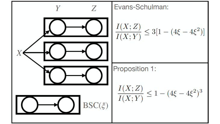
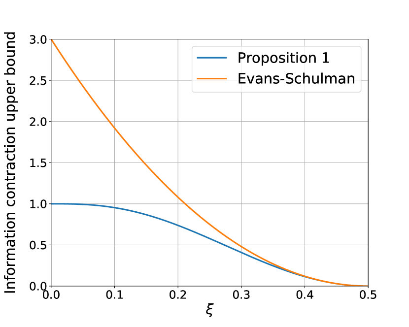
When n=1𝑛1n=1 and X𝑋X is a random bit, Proposition 1 gives the result of Theorem 1 in Evans and Schulman [10]. When n>1𝑛1n>1, Evans and Schulman proved a result in their paper (Lemma 2) which can be used to upper bound end-to-end information contraction. However, in the following we show that our contraction bound in Inequality (29) is strictly tighter than the one obtainable from the resutls of Evans and Schulman for n>1𝑛1n>1. In Figure 2, we give a simple example of a network which has a binary random variable X𝑋X as input, followed by three ξ𝜉\xi-noisy binary neurons. Let Y𝑌Y be the pre-noise output of these neurons, Z𝑍Z be the output after noise. Equivalently, we can consider that Z𝑍Z is the output of Y𝑌Y going through three independent BSCs of probability ξ𝜉\xi, as illustrated in Figure 2. Evans-Schulman method estimates the end-to-end information contraction upper bound to be 3[1(4ξ4ξ2)]3delimited-[]14𝜉4superscript𝜉23[1-(4\xi-4\xi^{2})] while Proposition 1 gives 1(4ξ4ξ2)31superscript4𝜉4superscript𝜉231-(4\xi-4\xi^{2})^{3}. More generally speaking, Evans-Schulman method gives an upper bound of nη𝑛𝜂n\eta and our estimate gives [1(1η)n]delimited-[]1superscript1𝜂𝑛[1-(1-\eta)^{n}] with η=1(4ξ4ξ2)𝜂14𝜉4superscript𝜉2\eta=1-(4\xi-4\xi^{2}). We have nη[1(1η)n]=0𝑛𝜂delimited-[]1superscript1𝜂𝑛0n\eta-[1-(1-\eta)^{n}]=0 while η=0𝜂0\eta=0, taking its derivative with respect to η𝜂\eta gives nn(1η)n1𝑛𝑛superscript1𝜂𝑛1n-n(1-\eta)^{n-1}, which is positive for any 0<η<10𝜂10<\eta<1. Hence nη>1(1η)n𝑛𝜂1superscript1𝜂𝑛n\eta>1-(1-\eta)^{n} for any 0<η<10𝜂10<\eta<1, the upper bound given by our Proposition 1 is always tighter than the one obtained from the Evans-Schulman method. In the limit where η0𝜂0\eta\rightarrow 0, the Evans-Schulman upper bound captures first order behavior of [1(1η)n]delimited-[]1superscript1𝜂𝑛[1-(1-\eta)^{n}].

Refer to caption
Refer to caption
Figure 2: Comparison of Evans-Schulman upper bound [10] (Lemma 2) with ours for a simple example network shown by the upper plot, the lower plot shows that our upper bound given by Proposition 1 is strictly tighter.

The authors would like to point out that similar results to Proposition 1 can be obtained from Theorem 5 of Polyanskiy and Wu [25], which has a very different proof from ours and uses percolation theory. Our proof using Theorem 1 also has the advantage of being applicable to more general situations where noise or failure is correlated between different neurons and not independent. Correlated neuron noise has been observed in biological [4] and physical science [26] contexts. Next we give some useful results derived from Theorem 1 taking into account the effect of weakly-correlated layer-wise neuron noise.

The most general form of Theorem 1 is not analytically tractable and requires the calculation of each pair of row-wise inner products of a 2nsuperscript2𝑛2^{n} by 2nsuperscript2𝑛2^{n} matrix 𝐀𝐀\mathbf{A}. However, we can consider a simplified model of layer-wise noise correlation by decomposing the noise to a shared noise source and an independent noise source. The shared noise is characterized by the probability ξ1subscript𝜉1\xi_{1} that all neurons in the layer fail together. Each neuron also has an independent noise source with an error probability of ξ2subscript𝜉2\xi_{2}. We consider that the two noise sources are combined in a successive way independent from one another. Intuitively speaking, first a biased coin is tossed to decide if all neurons of a layer will flip their output with probability ξ1subscript𝜉1\xi_{1} and then each neuron in that layer tosses its own coin to decide if it will flip its own output again with probability ξ2subscript𝜉2\xi_{2}. We have the following result under these assumptions.

Proposition 2.

Weakly-correlated layer-wise neuron noise.
Consider a layer composed of nnn noisy binary neurons that have a joint failure probability of ξ1subscriptξ1\xi_{1} and an independent individual failure probability of ξ2subscriptξ2\xi_{2} under our assumptions, the noise is weakly-correlated such that ξ11much-less-thansubscriptξ11\xi_{1}\ll 1 and ξ1ξ2much-less-thansubscriptξ1subscriptξ2\xi_{1}\ll\xi_{2}. Let XXX be the input to the binary neural network, YYY be the pre-noise output of the neurons and ZZZ be the output after noise. Then

I(X;Z)I(X;Y)1[(4ξ24ξ22)n+g(ξ2,n)ξ1]+𝒪(ξ1),𝐼𝑋𝑍𝐼𝑋𝑌1delimited-[]superscript4subscript𝜉24superscriptsubscript𝜉22𝑛𝑔subscript𝜉2𝑛subscript𝜉1𝒪subscript𝜉1\frac{I(X;Z)}{I(X;Y)}\leq 1-[(4\xi_{2}-4\xi_{2}^{2})^{n}+g(\xi_{2},n)\xi_{1}]+\mathchoice{{\scriptstyle\mathcal{O}}}{{\scriptstyle\mathcal{O}}}{{\scriptscriptstyle\mathcal{O}}}{\scalebox{0.6}{$\scriptscriptstyle\mathcal{O}$}}(\xi_{1}), (30)

where

g(ξ2,n)=2[(4ξ224ξ2+2)n(4ξ24ξ22)n].𝑔subscript𝜉2𝑛2delimited-[]superscript4superscriptsubscript𝜉224subscript𝜉22𝑛superscript4subscript𝜉24superscriptsubscript𝜉22𝑛g(\xi_{2},n)=2[\left(4\xi_{2}^{2}-4\xi_{2}+2\right)^{n}-\left(4\xi_{2}-4\xi_{2}^{2}\right)^{n}]. (31)
Proof.

The overall idea of this proof is similar to that of Proposition 1. The entries of matrix A are {(1ξ1)(1ξ2)nkξ2k+ξ1ξ2nk(1ξ2)k}0knsubscript1subscript𝜉1superscript1subscript𝜉2𝑛𝑘superscriptsubscript𝜉2𝑘subscript𝜉1superscriptsubscript𝜉2𝑛𝑘superscript1subscript𝜉2𝑘0𝑘𝑛\{(1-\xi_{1})(1-\xi_{2})^{n-k}\xi_{2}^{k}+\xi_{1}\xi_{2}^{n-k}(1-\xi_{2})^{k}\}_{0\leq k\leq n} with repetitions, taking into account the extra paths of transition introduced by the shared noise source. When ξ10subscript𝜉10\xi_{1}\rightarrow 0, they converge to simple binomial terms {ξ2k(1ξ2)nk}0knsubscriptsuperscriptsubscript𝜉2𝑘superscript1subscript𝜉2𝑛𝑘0𝑘𝑛\{\xi_{2}^{k}(1-\xi_{2})^{n-k}\}_{0\leq k\leq n} which are strongly ordered as shown previously in the proof of Proposition 1. A continuity argument with respect to ξ1subscript𝜉1\xi_{1} gives that the ordering is preserved for small enough ξ1subscript𝜉1\xi_{1}. Thus rearrangement inequality still applies and each term in the reversed order product is (to the leading order in ξ1subscript𝜉1\xi_{1})

(1ξ2)nξ2n2ξ1(1ξ2)nξ2n+2ξ1(1ξ2)2(nk)ξ22k.superscript1subscript𝜉2𝑛superscriptsubscript𝜉2𝑛2subscript𝜉1superscript1subscript𝜉2𝑛superscriptsubscript𝜉2𝑛2subscript𝜉1superscript1subscript𝜉22𝑛𝑘superscriptsubscript𝜉22𝑘(1-\xi_{2})^{n}\xi_{2}^{n}-2\xi_{1}(1-\xi_{2})^{n}\xi_{2}^{n}+2\xi_{1}(1-\xi_{2})^{2(n-k)}\xi_{2}^{2k}. (32)

And the sum is lower bounded as (to the leading order in ξ1subscript𝜉1\xi_{1})

j=12nak,ja,j(1ξ1)(4ξ24ξ22)n/2+superscriptsubscript𝑗1superscript2𝑛subscript𝑎𝑘𝑗subscript𝑎𝑗limit-from1subscript𝜉1superscript4subscript𝜉24superscriptsubscript𝜉22𝑛2\displaystyle\sum_{j=1}^{2^{n}}\sqrt{a_{k,j}a_{\ell,j}}\geq(1-\xi_{1})(4\xi_{2}-4\xi_{2}^{2})^{n/2}+
ξ1(ξ2ξ22)n/2k=0n(nk)[(1ξ2)2]nk(ξ22)ksubscript𝜉1superscriptsubscript𝜉2superscriptsubscript𝜉22𝑛2superscriptsubscript𝑘0𝑛binomial𝑛𝑘superscriptdelimited-[]superscript1subscript𝜉22𝑛𝑘superscriptsuperscriptsubscript𝜉22𝑘\displaystyle\frac{\xi_{1}}{(\xi_{2}-\xi_{2}^{2})^{n/2}}\sum_{k=0}^{n}{n\choose k}[(1-\xi_{2})^{2}]^{n-k}(\xi_{2}^{2})^{k}
=(1ξ1)(4ξ24ξ22)n/2+ξ1(ξ2ξ22)n/2[2ξ222ξ2+1]n.absent1subscript𝜉1superscript4subscript𝜉24superscriptsubscript𝜉22𝑛2subscript𝜉1superscriptsubscript𝜉2superscriptsubscript𝜉22𝑛2superscriptdelimited-[]2superscriptsubscript𝜉222subscript𝜉21𝑛\displaystyle=(1-\xi_{1})(4\xi_{2}-4\xi_{2}^{2})^{n/2}+\frac{\xi_{1}}{(\xi_{2}-\xi_{2}^{2})^{n/2}}[2\xi_{2}^{2}-2\xi_{2}+1]^{n}. (33)

Applying Theorem 1 with the above inequality proves the proposition. ∎

The information contraction upper bound in Proposition 2 can be compared with the bound in Proposition 1. We have the following corollary comparing their magnitudes.

Corollary 1.

At the same per neuron noise level between the case of independent noise and the case of weakly-correlated noise, meaning ξ1(1ξ2)+(1ξ1)ξ2=ξsubscript𝜉11subscript𝜉21subscript𝜉1subscript𝜉2𝜉\xi_{1}(1-\xi_{2})+(1-\xi_{1})\xi_{2}=\xi, let ηind(ξ)subscript𝜂ind𝜉\eta_{\mathrm{ind}}(\xi) denote the information contraction upper bound for independent neuron noise in Proposition 1 and let ηwc(ξ1,ξ2)subscript𝜂wcsubscript𝜉1subscript𝜉2\eta_{\mathrm{wc}}(\xi_{1},\xi_{2}) denote the information contraction upper bound for weakly-correlated neuron noise in Proposition 2. In the weakly-correlated noise limit where ξ11much-less-thansubscript𝜉11\xi_{1}\ll 1 and ξ1ξ2much-less-thansubscript𝜉1subscript𝜉2\xi_{1}\ll\xi_{2}, we have

ηwc(ξ1,ξ2)ηind(ξ).subscript𝜂wcsubscript𝜉1subscript𝜉2subscript𝜂ind𝜉\eta_{\mathrm{wc}}(\xi_{1},\xi_{2})\leq\eta_{\mathrm{ind}}(\xi). (34)
Proof.

Plug the expression ξ1(1ξ2)+(1ξ1)ξ2=ξsubscript𝜉11subscript𝜉21subscript𝜉1subscript𝜉2𝜉\xi_{1}(1-\xi_{2})+(1-\xi_{1})\xi_{2}=\xi into Proposition 1 and expand (4ξ4ξ2)nsuperscript4𝜉4superscript𝜉2𝑛(4\xi-4\xi^{2})^{n} to leading order in ξ1subscript𝜉1\xi_{1}. We have

ηind(ξ)=1[(4ξ24ξ22)n+g~(ξ2,n)ξ1]+𝒪(ξ1),subscript𝜂ind𝜉1delimited-[]superscript4subscript𝜉24superscriptsubscript𝜉22𝑛~𝑔subscript𝜉2𝑛subscript𝜉1𝒪subscript𝜉1\eta_{\mathrm{ind}}(\xi)=1-[(4\xi_{2}-4\xi_{2}^{2})^{n}+\tilde{g}(\xi_{2},n)\xi_{1}]+\mathchoice{{\scriptstyle\mathcal{O}}}{{\scriptstyle\mathcal{O}}}{{\scriptscriptstyle\mathcal{O}}}{\scalebox{0.6}{$\scriptscriptstyle\mathcal{O}$}}(\xi_{1}), (35)

with g~(ξ2,n)=4n(2ξ21)2(4ξ24ξ22)n1~𝑔subscript𝜉2𝑛4𝑛superscript2subscript𝜉212superscript4subscript𝜉24superscriptsubscript𝜉22𝑛1\tilde{g}(\xi_{2},n)=4n(2\xi_{2}-1)^{2}(4\xi_{2}-4\xi_{2}^{2})^{n-1}. Function g(ξ2,n)𝑔subscript𝜉2𝑛g(\xi_{2},n) can be factorized as g(ξ2,n)=4(4ξ224ξ2+1)[i=1n(4ξ224ξ2+2)ni(4ξ24ξ22)i1]𝑔subscript𝜉2𝑛44superscriptsubscript𝜉224subscript𝜉21delimited-[]superscriptsubscript𝑖1𝑛superscript4superscriptsubscript𝜉224subscript𝜉22𝑛𝑖superscript4subscript𝜉24superscriptsubscript𝜉22𝑖1g(\xi_{2},n)=4(4\xi_{2}^{2}-4\xi_{2}+1)[\sum_{i=1}^{n}(4\xi_{2}^{2}-4\xi_{2}+2)^{n-i}(4\xi_{2}-4\xi_{2}^{2})^{i-1}] for n1𝑛1n\geq 1. Since 4ξ224ξ2+24ξ24ξ224superscriptsubscript𝜉224subscript𝜉224subscript𝜉24superscriptsubscript𝜉224\xi_{2}^{2}-4\xi_{2}+2\geq 4\xi_{2}-4\xi_{2}^{2} for 0ξ20.50subscript𝜉20.50\leq\xi_{2}\leq 0.5, thus we have g(ξ2,n)4(2ξ21)2n(4ξ24ξ22)n1=g~(ξ2,n)𝑔subscript𝜉2𝑛4superscript2subscript𝜉212𝑛superscript4subscript𝜉24superscriptsubscript𝜉22𝑛1~𝑔subscript𝜉2𝑛g(\xi_{2},n)\geq 4(2\xi_{2}-1)^{2}n(4\xi_{2}-4\xi_{2}^{2})^{n-1}=\tilde{g}(\xi_{2},n) and the corollary is proven by comparing Equation (35) with Equation (30). ∎

Refer to caption
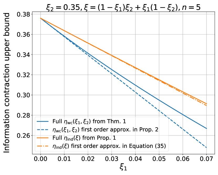
Figure 3: A numerical comparison of the information contraction upper bound for independent noise and weakly-correlated layer-wise neuron noise with ξ2=0.35subscript𝜉20.35\xi_{2}=0.35 and n=5𝑛5n=5. Weakly-correlated noise results in a lower contraction ratio upper bound than independent noise as stated in Corollary 1.

Here we give a numerical example to illustrate these results. Figure 3 shows a comparison between the case of independent noise and the case of weakly-correlated noise for a layer of n=5𝑛5n=5 neurons and ξ2=0.35subscript𝜉20.35\xi_{2}=0.35. It is numerically verifiable that the ordering of terms is preserved for ξ1subscript𝜉1\xi_{1} up to 0.070.070.07 and ηwcsubscript𝜂wc\eta_{\mathrm{wc}} can be evaluated directly from Theorem 1 by calculating the reversed-order sum of products. Our leading order result in Proposition 2 gives a good approximation in the small ξ1subscript𝜉1\xi_{1} limit. Weakly-correlated neuron noise leads to a lower end-to-end information contraction upper bound as stipulated by Corollary 1.

IV Application to noisy neural networks

In this section, we apply the SDPI results obtained in the previous section to study the end-to-end information contraction in a neural network. We will only have formal results for the case of independent noise in the rest of this paper, whenever we say that a component is ξ𝜉\xi-noisy, it implies that its failure is independent. Theorem 2 gives the main result by successively applying Proposition 1 to each layer.
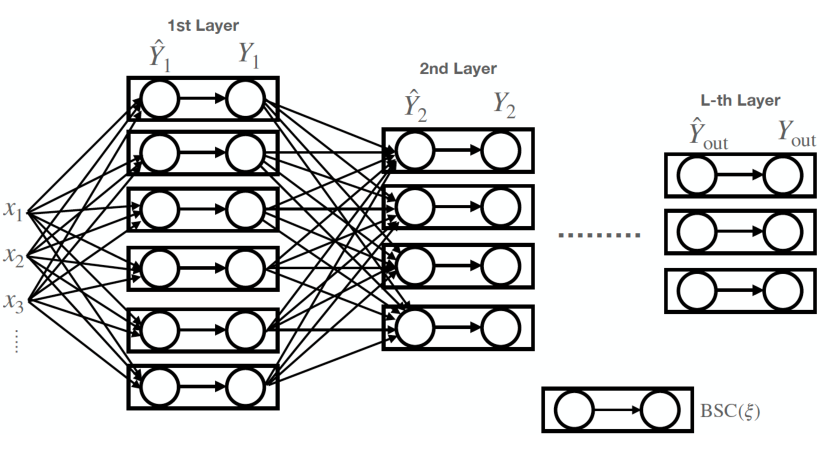
Refer to caption
Figure 4: Schematic of a noisy neural network with ξ𝜉\xi-noisy binary neurons.
Theorem 2.

Information decay in a noisy neural network
In a feed-forward simply layered fully-connected binary neural network composed of LLL layers of ξξ\xi-noisy neurons, let XXX be any subset of input to the neural network and YoutsubscriptYoutY_{\mathrm{out}} be the output, then

I(X;Yout)=1L[1(4ξ4ξ2)n]H(X),𝐼𝑋subscript𝑌outsuperscriptsubscriptproduct1𝐿delimited-[]1superscript4𝜉4superscript𝜉2subscript𝑛𝐻𝑋I(X;Y_{\mathrm{out}})\leq\prod_{\ell=1}^{L}\left[1-(4\xi-4\xi^{2})^{n_{\ell}}\right]H(X), (36)

where nsubscript𝑛n_{\ell} is the number of neurons in layer \ell.

Proof.

We prove the theorem by a mathematical induction on the number of layers L𝐿L. Figure 4 gives a schematic of a noisy neural network, let Ysubscript𝑌Y_{\ell} denote the output activations of noisy neurons at layer \ell and Y^subscript^𝑌\hat{Y}_{\ell} denote its pre-noise values. We have therefore a Markov chain connecting the input to the output of the network: XY^1Y1Y^2Y2Y^L1YL1Y^outYout𝑋subscript^𝑌1subscript𝑌1subscript^𝑌2subscript𝑌2subscript^𝑌L1subscript𝑌L1subscript^𝑌outsubscript𝑌outX\rightarrow\hat{Y}_{1}\rightarrow Y_{1}\rightarrow\hat{Y}_{2}\rightarrow Y_{2}\rightarrow...\rightarrow\hat{Y}_{\mathrm{L-1}}\rightarrow Y_{\mathrm{L-1}}\rightarrow\hat{Y}_{\mathrm{out}}\rightarrow Y_{\mathrm{out}}. When L=1𝐿1L=1, applying Proposition 1 gives I(X;Yout)[1(4ξ4ξ2)n1]I(X;Y^out)𝐼𝑋subscript𝑌outdelimited-[]1superscript4𝜉4superscript𝜉2subscript𝑛1𝐼𝑋subscript^𝑌outI(X;Y_{\mathrm{out}})\leq[1-(4\xi-4\xi^{2})^{n_{1}}]I(X;\hat{Y}_{\mathrm{out}}) and by definition I(X;Y^out)H(X)𝐼𝑋subscript^𝑌out𝐻𝑋I(X;\hat{Y}_{\mathrm{out}})\leq H(X). Hence we have I(X;Yout)[1(4ξ4ξ2)n1]H(X)𝐼𝑋subscript𝑌outdelimited-[]1superscript4𝜉4superscript𝜉2subscript𝑛1𝐻𝑋I(X;Y_{\mathrm{out}})\leq[1-(4\xi-4\xi^{2})^{n_{1}}]H(X). Now suppose that the claim is true up to a layer number of K𝐾K with K1𝐾1K\geq 1, then for L=K+1𝐿𝐾1L=K+1, we have I(X;Yout)[1(4ξ4ξ2)nK+1]I(X;Y^out)𝐼𝑋subscript𝑌outdelimited-[]1superscript4𝜉4superscript𝜉2subscript𝑛𝐾1𝐼𝑋subscript^𝑌outI(X;Y_{\mathrm{out}})\leq[1-(4\xi-4\xi^{2})^{n_{K+1}}]I(X;\hat{Y}_{\mathrm{out}}). Since XYKY^out𝑋subscript𝑌𝐾subscript^𝑌outX\rightarrow Y_{K}\rightarrow\hat{Y}_{\mathrm{out}}, data processing inequality gives I(X;Y^out)I(X;YK)𝐼𝑋subscript^𝑌out𝐼𝑋subscript𝑌𝐾I(X;\hat{Y}_{\mathrm{out}})\leq I(X;Y_{K}). Treating the first K𝐾K layers as a new neural network and applying the inductive hypothesis give I(X;YK)=1K[1(4ξ4ξ2)n]H(X)𝐼𝑋subscript𝑌𝐾superscriptsubscriptproduct1𝐾delimited-[]1superscript4𝜉4superscript𝜉2subscript𝑛𝐻𝑋I(X;Y_{K})\leq\prod_{\ell=1}^{K}\left[1-(4\xi-4\xi^{2})^{n_{\ell}}\right]H(X), therefore I(X;Yout)=1K+1[1(4ξ4ξ2)n]H(X)𝐼𝑋subscript𝑌outsuperscriptsubscriptproduct1𝐾1delimited-[]1superscript4𝜉4superscript𝜉2subscript𝑛𝐻𝑋I(X;Y_{\mathrm{out}})\leq\prod_{\ell=1}^{K+1}\left[1-(4\xi-4\xi^{2})^{n_{\ell}}\right]H(X) and we conclude the proof by induction. ∎

Theorem 2 relates the rate of information contraction in a noisy neural network to its layer width and overall depth. It implies that wider and shallower noisy neural networks are less susceptible to the decay in information, which rigorizes the intuition that a wider width provides more redundant paths for information to flow through and a deeper depth results in more irrevocable loss. More importantly, Theorem 2 gives an upper bound for such loss that is tighter than previous results. Applying Evans-Schulman method leads to a bound which is the sum over all possible paths from X𝑋X to the output and Theorem 2 is considerably tighter. In the more special cases where the connections are not dense in the hidden layers on paths from X𝑋X to the output, the upper bound in Theorem 2 can be further tightened by only requiring the number of neurons in each layer that are connected to X𝑋X.

Using a noisy neural network to compute functions becomes more challenging with a rising level of noise as a result of this information contraction, and there is a point beyond which reliable computation is no longer possible. Fano’s inequality gives a lower bound on the minimum mutual information required for reliable computation. The intuition is that if the output is a function of the input with a high probability then their mutual information must be high as well. The following corollary summarizes this result.

Corollary 2.

If a feed-forward simply layered binary neural network with L𝐿L layers of ξ𝜉\xi-noisy neurons computes a non-constant function δ𝛿\delta-reliably (that is, it produces the correct output for any network input with probability at least 1δ1𝛿1-\delta where δ<1/2𝛿12\delta<1/2). Then

=1L1[1(4ξ4ξ2)n][1(4ξ4ξ2)]Δ,superscriptsubscriptproduct1𝐿1delimited-[]1superscript4𝜉4superscript𝜉2subscript𝑛delimited-[]14𝜉4superscript𝜉2Δ\prod_{\ell=1}^{L-1}\left[1-(4\xi-4\xi^{2})^{n_{\ell}}\right]\left[1-(4\xi-4\xi^{2})\right]\geq\Delta, (37)

with

Δ=1+δlog2δ+(1δ)log2(1δ).Δ1𝛿subscript2𝛿1𝛿subscript21𝛿\Delta=1+\delta\log_{2}\delta+(1-\delta)\log_{2}(1-\delta). (38)
Proof.

The neural network implements a non-trivial function of its input, therefore at least one of its output neurons outputs a non-constant Boolean function f𝑓f of the network input, now we can restrict the proof to this particular output neuron. Obviously the computation of f𝑓f needs to be at least δ𝛿\delta-reliable. f𝑓f depends on at least one of the input to be non-constant. Let xisubscript𝑥𝑖x_{i} denote an input that f𝑓f depends on, there exists a setting of the other n1𝑛1n-1 input variables {ck}kisubscriptsubscript𝑐𝑘𝑘𝑖\left\{c_{k}\right\}_{k\neq i} such that f(c1,c2,,ci1,xi,ci+1,,cn)𝑓subscript𝑐1subscript𝑐2subscript𝑐𝑖1subscript𝑥𝑖subscript𝑐𝑖1subscript𝑐𝑛f(c_{1},c_{2},...,c_{i-1},x_{i},c_{i+1},...,c_{n}) is either xisubscript𝑥𝑖x_{i} or x¯isubscript¯𝑥𝑖\bar{x}_{i}. Let y𝑦y be the random variable measured at the output of that neuron for xisubscript𝑥𝑖x_{i} being a uniformly distributed binary random variable and other inputs to the neural network set to {ck}kisubscriptsubscript𝑐𝑘𝑘𝑖\left\{c_{k}\right\}_{k\neq i}. We apply a decoding function to decode xisubscript𝑥𝑖x_{i} from y𝑦y: x^i=ysubscript^𝑥𝑖𝑦\hat{x}_{i}=y or x^i=y¯subscript^𝑥𝑖¯𝑦\hat{x}_{i}=\bar{y} depending on if f(c1,c2,,ci1,xi,ci+1,,cn)𝑓subscript𝑐1subscript𝑐2subscript𝑐𝑖1subscript𝑥𝑖subscript𝑐𝑖1subscript𝑐𝑛f(c_{1},c_{2},...,c_{i-1},x_{i},c_{i+1},...,c_{n}) is xisubscript𝑥𝑖x_{i} or x¯isubscript¯𝑥𝑖\bar{x}_{i}. Let e𝑒e represent occurrence of a decoding error: x^ixisubscript^𝑥𝑖subscript𝑥𝑖\hat{x}_{i}\neq x_{i}. Fano’s inequality [27] gives I(xi;y)=H(xi)H(xi|y)H(xi)H(e)P(e)log2(|𝒳|1)𝐼subscript𝑥𝑖𝑦𝐻subscript𝑥𝑖𝐻conditionalsubscript𝑥𝑖𝑦𝐻subscript𝑥𝑖𝐻𝑒𝑃𝑒subscript2𝒳1I(x_{i};y)=H(x_{i})-H(x_{i}|y)\geq H(x_{i})-H(e)-P(e)\log_{2}(|\mathcal{X}|-1), where P(e)𝑃𝑒P(e) is the probability of a decoding error, H(e)=P(e)log2(P(e))(1P(e))log2(1P(e))𝐻𝑒𝑃𝑒subscript2𝑃𝑒1𝑃𝑒subscript21𝑃𝑒H(e)=-P(e)\log_{2}(P(e))-(1-P(e))\log_{2}(1-P(e)) the corresponding binary entropy and 𝒳=2𝒳2\mathcal{X}=2 is the support of xisubscript𝑥𝑖x_{i}. Recall that y𝑦y is a δ𝛿\delta-reliable representation of f(c1,c2,,ci1,xi,ci+1,,cn)𝑓subscript𝑐1subscript𝑐2subscript𝑐𝑖1subscript𝑥𝑖subscript𝑐𝑖1subscript𝑐𝑛f(c_{1},c_{2},...,c_{i-1},x_{i},c_{i+1},...,c_{n}), hence P(e)δ𝑃𝑒𝛿P(e)\leq\delta and I(xi;y)1+δlog2δ+(1δ)log2(1δ)𝐼subscript𝑥𝑖𝑦1𝛿subscript2𝛿1𝛿subscript21𝛿I(x_{i};y)\geq 1+\delta\log_{2}\delta+(1-\delta)\log_{2}(1-\delta). Finally we apply Theorem 2 to the subset of neural network that starts from xisubscript𝑥𝑖x_{i} and ends at y𝑦y and we have =1L1[1(4ξ4ξ2)n][1(4ξ4ξ2)]I(xi;y)1+δlog2δ+(1δ)log2(1δ)superscriptsubscriptproduct1𝐿1delimited-[]1superscript4𝜉4superscript𝜉2subscript𝑛delimited-[]14𝜉4superscript𝜉2𝐼subscript𝑥𝑖𝑦1𝛿subscript2𝛿1𝛿subscript21𝛿\prod_{\ell=1}^{L-1}\left[1-(4\xi-4\xi^{2})^{n_{\ell}}\right]\left[1-(4\xi-4\xi^{2})\right]\geq I(x_{i};y)\geq 1+\delta\log_{2}\delta+(1-\delta)\log_{2}(1-\delta). ∎

Sometimes it is useful to consider the situation where the noisy neural network is used as a feature extractor and the output of the network can then be further processed to calculate a Boolean function δ𝛿\delta-reliably. In this case, the inequality becomes =1L[1(4ξ4ξ2)n]Δsuperscriptsubscriptproduct1𝐿delimited-[]1superscript4𝜉4superscript𝜉2subscript𝑛Δ\prod_{\ell=1}^{L}\left[1-(4\xi-4\xi^{2})^{n_{\ell}}\right]\geq\Delta and no longer limited by a single noisy channel in the output neuron.

With Corollary 2, we proceed to give a lower bound for the number of noisy neurons for reliable computation. We begin by proving a lemma which will be used in the proof of our next theorem.

Lemma 2.

Given L𝐿L strictly positive integers n1subscript𝑛1n_{1}, n2subscript𝑛2n_{2}, …, nsubscript𝑛n_{\ell} and 0a10𝑎10\leq a\leq 1, then

=1L(1an)(1a=1LnL)L.superscriptsubscriptproduct1𝐿1superscript𝑎subscript𝑛superscript1superscript𝑎superscriptsubscript1𝐿subscript𝑛𝐿𝐿\prod_{\ell=1}^{L}(1-a^{n_{\ell}})\leq(1-a^{\frac{\sum_{\ell=1}^{L}n_{\ell}}{L}})^{L}. (39)
Proof.

We use the inequality of arithmetic and geometric means to prove this lemma. First notice that 1an1superscript𝑎subscript𝑛1-a^{n_{\ell}} is non-negative for 0a10𝑎10\leq a\leq 1 and we can apply the inequality of arithmetic and geometric means to the product on the left hand side, and we have

=1L(1an)[L=1LanL]L(1a=1LnL)L,superscriptsubscriptproduct1𝐿1superscript𝑎subscript𝑛superscriptdelimited-[]𝐿superscriptsubscript1𝐿superscript𝑎subscript𝑛𝐿𝐿superscript1superscript𝑎superscriptsubscript1𝐿subscript𝑛𝐿𝐿\prod_{\ell=1}^{L}(1-a^{n_{\ell}})\leq\left[\frac{L-\sum_{\ell=1}^{L}a^{n_{\ell}}}{L}\right]^{L}\leq(1-a^{\frac{\sum_{\ell=1}^{L}n_{\ell}}{L}})^{L}, (40)

where we have applied the inequality a second time for the sum =1Lan/Lsuperscriptsubscript1𝐿superscript𝑎subscript𝑛𝐿\sum_{\ell=1}^{L}a^{n_{\ell}}/L. Equality is attained when all the nsubscript𝑛n_{\ell} are equal: n1=n2==nsubscript𝑛1subscript𝑛2subscript𝑛n_{1}=n_{2}=...=n_{\ell}. ∎

Lemma 2 can be used to bound the information contraction ratio in a noisy neural network. Particularly, it implies that the contraction upper bound is highest when the neurons are equally partitioned among all hidden layers. More importantly, it connects the information contraction ratio with the total number of neurons in the network, which leads to the following theorem

Theorem 3.

If a feed-forward simply layered binary neural network with L𝐿L layers of ξ𝜉\xi-noisy neurons computes a non-constant function δ𝛿\delta-reliably, then its total number of hidden layer noisy neurons N𝑁N satisfies

NNs(ξ,δ,L),𝑁subscript𝑁𝑠𝜉𝛿𝐿N\geq N_{s}(\xi,\delta,L), (41)

with

Ns(ξ,δ,L)=(L1)log(1(Δ1(4ξ4ξ2))1/(L1))log(4ξ4ξ2).subscript𝑁𝑠𝜉𝛿𝐿𝐿11superscriptΔ14𝜉4superscript𝜉21𝐿14𝜉4superscript𝜉2N_{s}(\xi,\delta,L)=\displaystyle\frac{(L-1)\log\left(1-\left(\displaystyle\frac{\Delta}{1-(4\xi-4\xi^{2})}\right)^{1/(L-1)}\right)}{\log(4\xi-4\xi^{2})}. (42)
Proof.

In Corollary 2, applying Lemma 2 to the left hand side of Inequality (37) gives

=1L1[1an](1a)[1a=1L1n/(L1)]L1(1a),superscriptsubscriptproduct1𝐿1delimited-[]1superscript𝑎subscript𝑛1𝑎superscriptdelimited-[]1superscript𝑎superscriptsubscript1𝐿1subscript𝑛𝐿1𝐿11𝑎\prod_{\ell=1}^{L-1}\left[1-a^{n_{\ell}}\right](1-a)\leq\left[1-a^{\sum_{\ell=1}^{L-1}n_{\ell}/(L-1)}\right]^{L-1}(1-a), (43)

with

0a=4ξ4ξ21.0𝑎4𝜉4superscript𝜉210\leq a=4\xi-4\xi^{2}\leq 1. (44)

Corollary 2 gives

(1aNL1)L1(1a)Δ.superscript1superscript𝑎𝑁𝐿1𝐿11𝑎Δ\left(1-a^{\frac{N}{L-1}}\right)^{L-1}(1-a)\geq\Delta. (45)

Rearranging terms and taking the logarithmic give

log(1(Δ1a)1/(L1))NL1loga.1superscriptΔ1𝑎1𝐿1𝑁𝐿1𝑎\log\left(1-\left(\frac{\Delta}{1-a}\right)^{1/(L-1)}\right)\geq\frac{N}{L-1}\log a. (46)

Since loga0𝑎0\log a\leq 0, therefore

N(L1)log(1(Δ1a)1/(L1))loga.𝑁𝐿11superscriptΔ1𝑎1𝐿1𝑎N\geq\frac{(L-1)\log\left(1-\left(\frac{\Delta}{1-a}\right)^{1/(L-1)}\right)}{\log a}. (47)

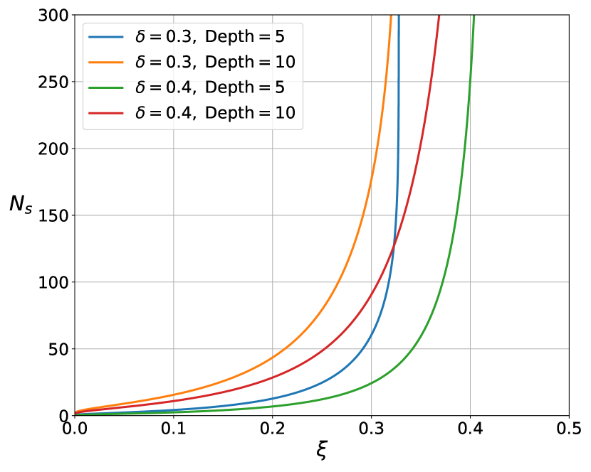
In Figure 5, we show how this lower bound grows with the noise level ξ𝜉\xi. The minimum number of neurons required grows quickly when ξ𝜉\xi approaches δ𝛿\delta. Equation (42) gives that Nssubscript𝑁𝑠N_{s} approaches infinity when Δ=1(4ξ4ξ2)Δ14𝜉4superscript𝜉2\Delta=1-(4\xi-4\xi^{2}). This is because that information flow is limited by the last noisy neuron which is the output. The cutoff ξ𝜉\xi is actually slightly higher than δ𝛿\delta for δ<0.5𝛿0.5\delta<0.5. We believe that this is an artifact of taking the upper bounds that cannot be attained in these cases. Another important fact is that at fixed δ𝛿\delta and ξ𝜉\xi, Nssubscript𝑁𝑠N_{s} increases monotonically with the number of layers L𝐿L, which is showcased in Figure 5 as well.
Refer to caption
Figure 5: Lower bounds for number of neurons Nssubscript𝑁𝑠N_{s} in Theorem 3 as a function of the noiseness of neurons evaluated for different computation reliability requirements and network depths.

This particular trade-off between the depth of the noisy network and the number of neurons goes in the opposite direction to various no-flattening results for neural networks and circuits. In terms of expressibility, many depth-width trade-off relationships suggest that flattening or reducing the depth of a network is neuron inefficient. It takes more (sometimes exponentially more) neurons to implement the same function, if limited to arranging them in a smaller number of layers. These results are used as arguments to explain why “deep” learning works so well [28]. There are similar results in circuit complexity suggesting that “depth” helps. For example, the famous result that Parity𝐀𝐂0Paritysuperscript𝐀𝐂0\textit{Parity}\not\in\mathbf{AC}^{0} by Furst et al. [29] and Håstad [30] suggests that implementing the parity function (n element XOR function) over AND, NOT, OR gates of unlimited fan-in costs an exponential number of gates (as a function of input number n𝑛n) if limited to a depth d𝑑d, while there are solutions with linear cost in the number of gates when they are arranged in a tree of depth logarithmic in n𝑛n. Usually these no-flattening results can be expressed as a size complexity function Ω(n,d)Ω𝑛𝑑\Omega(n,d) being a lower bound for the number of neurons/gates, which increases with depth d𝑑d. We have the following corollary combining these results with Theorem 3.

Corollary 3.

Let f𝑓f be an n𝑛n-input Boolean function of size complexity Ω(n,d)Ω𝑛𝑑\Omega(n,d) lower bound in the class of Threshold Circuits (TC, circuits composed of threshold gates or binary neurons with unbounded fan-in and fan-out), suppose that a feed-forward simply layered binary neural network implements function f𝑓f and is δ𝛿\delta-reliable up to a neuron noise level of ξ𝜉\xi, then at a maximum depth D𝐷D, the minimum number of neurons required in this network is

min1dDmax(Ω(n,d),Ns(ξ,δ,d)+1).subscript1𝑑𝐷Ω𝑛𝑑subscript𝑁𝑠𝜉𝛿𝑑1\min_{1\leq d\leq D}\max\left(\Omega(n,d),N_{s}(\xi,\delta,d)+1\right). (48)

Corollary 3 recognizes that in order for a network to have both enough expressive power and noise robustness, it needs to satisfy both minimum size requirements. The +11+1 accounts for the last output neuron. Nssubscript𝑁𝑠N_{s} monotonically increases with the network depth and ΩΩ\Omega monotonically decreases with the network depth. When they cross each other, there is an optimal depth that gives the minimum size complexity requirement. Intuitively, the network cannot be too long and thin since it cannot be noise resistant enough as we have shown; and nor can it be too shallow as the expressibility requirement makes it very neuron inefficient. The function Ω(n,d)Ω𝑛𝑑\Omega(n,d) is f𝑓f-dependent and are obtained from circuit complexity theory of the complexity class TC. The complexity lower bound study of class TC is currently a frontier field of research and many efforts are still on-going [31]. We give an example for f𝑓f being the parity function defined as

f(x)=x1x2xn,𝑓𝑥direct-sumsubscript𝑥1subscript𝑥2subscript𝑥𝑛f(x)=x_{1}\oplus x_{2}\oplus...\oplus x_{n}, (49)

where direct-sum\oplus denotes XOR. Impagliazzo et al. [22] proved that any threshold circuit of depth d𝑑d that computes the parity function has at least (n/2)1/2(d1)superscript𝑛212𝑑1(n/2)^{1/2(d-1)} threshold gates or binary neurons in our terminology. Therefore, we can have Ω(n,d)=(n/2)1/2(d1)Ω𝑛𝑑superscript𝑛212𝑑1\Omega(n,d)=(n/2)^{1/2(d-1)}, which holds as the absolute lower bound on the number of neurons. It may be possible to further improve it, since we restrict the network structure to be simply layered.
Refer to caption
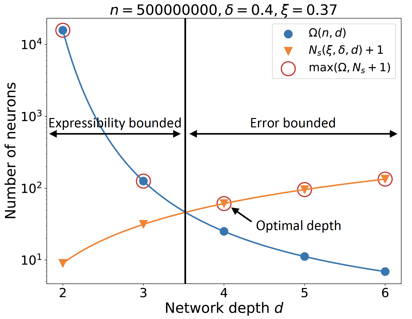
Figure 6: Minimum number of neurons required according to Corollary 3 for the parity function, blue dots are the size complexity bounds for the parity function Ω(n,d)=(n/2)1/2(d1)Ω𝑛𝑑superscript𝑛212𝑑1\Omega(n,d)=(n/2)^{1/2(d-1)} and orange triangles are the noise robustness bounds. The minimum number of neurons required needs to be more than the maximum of both bounds, which are shown by red circles.

Figure 6 shows a case for the parity function with n=5×10⁸𝑛5superscript108n=5\times 10^{8}, δ=0.4𝛿0.4\delta=0.4, ξ=0.37𝜉0.37\xi=0.37. Ω(n,d)Ω𝑛𝑑\Omega(n,d) (blue curve) monotonically decreases with d𝑑d and Ns+1subscript𝑁𝑠1N_{s}+1 (orange curve) monotonically increases with d𝑑d. The crossing happens between d=3𝑑3d=3 and d=4𝑑4d=4. To the left of this crossing point, the minimum number of neurons required is limited by the required expressive power of the network and to the right of this crossing point it is limited by the noise robustness requirement. There are therefore two distinct regimes where one is expressibility bounded and the other is error bounded. The optimal number of layers that achieves the minimum neuron number requirement in this case is 444 with a minimum lower bound of 61.2261.2261.22 neurons. (Note that as we are obtaining results from bounds that are not necessarily tight, the actual optimal number might be different.) This is almost a ten-fold increase from the minimum requirement in the absence of noise for d6𝑑6d\leq 6 which is Ω(n,6)=6.915Ω𝑛66.915\Omega(n,6)=6.915. Performing computation with noisy neurons while retaining noise-robustness requires using more neurons. Our paper gives a lower bound for such increase.

The results we have derived in this section can be extended to the case of weakly-correlated layer-wise neuron noise using Proposition 2. Qualitatively speaking, Corollary 1 indicates that weakly-correlated neuron noise results in an end-to-end information contraction upper bound that is lower than the independent noise case at equal ξ𝜉\xi, thus requiring a further increase in the minimum number of neurons to combat loss of information.

One way to understand this increase of the number of neurons is via considering error correction mechanism. As the gates becomes noisy, each logical bit of information would require multiple physical bits to encode so that the robustness condition can be satisfied, which is similar to the error-correction overhead that we will discuss the next.

V Application to fault-tolerant cellular automata

Since the early works of Turing [32], people are interested in the “self-organization” phenomena, where stable patterns form in a dynamical system, despite dissipation and noise. In the language of statistical physics, these stable patterns can be regarded as phases of the system at a finite temperature [18]; while to computer scientists, the fact that different initial conditions can lead to unique different patterns means that information can be reliably stored in these complex systems, which serve as fault-tolerant memory. A simplified model for studying these phenomena, adopted by both statistical physics [18, 19, 20] and computer scientists [15, 16, 17], is the cellular automata [19], where time and space are both discrete, similar to the binary neurons being considered in this paper. In fact, similar to Von Neumann’s circuit approach, fault-tolerant cellular automata form another class of model capable of reliable universal computation with unreliable components [15]. More recently, these systems are also found to be connected to a novel phase of matter called time-crystals [21].
Refer to caption
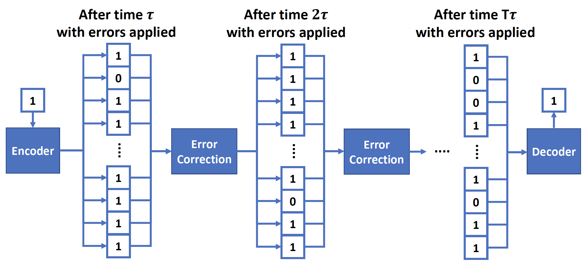
Figure 7: Schematic of fault-tolerant memory with error correction, the system is unrolled in time dimension, it corresponds to the same physical memory array. τ𝜏\tau is the time between two consecutive memory “refreshes”. One logical bit is protected over a long period of time despite continuous corruption by random noise that happens to physical memory bits.

In this section, we apply our information contraction results to fault-tolerant cellular automata with any (global or local) update rules. For simplicity, we consider the capability of these systems serving as fault-tolerant memory. Without loss of generality, we assume that such systems encode 1 bit of information with n𝑛n noisy physical memory bits and apply some error correction rules at constant intervals of time (a time step of τ𝜏\tau) only using information stored in noisy physical memory bits, meanwhile errors may occur randomly in these memory cells. Our approach may apply to wider classes of systems, however, in this paper we will consider fault-tolerant cellular automata [15] as an example of fault-tolerant memory.

An important question to ask is: given ξ𝜉\xi-noisy memory cells, what is the minimum memory overhead n(δ,T,ξ)𝑛𝛿𝑇𝜉n(\delta,T,\xi) required such that 1 bit of logical information can be δ𝛿\delta-reliably retrieved (correctly decoded with probability at least 1δ1𝛿1-\delta) after T𝑇T intervals in time? This time duration T(δ,n,ξ)𝑇𝛿𝑛𝜉T(\delta,n,\xi) (normalized by τ𝜏\tau) with δ𝛿\delta being a constant (e.g. 2/3232/3 as in [15]) is also called the relaxation time of the system. While any finite system has a finite relaxation time, stable phases in statistical physics are defined as the case of T(δ,n,ξ)𝑇𝛿𝑛𝜉T(\delta,n,\xi)\to\infty at the thermodynamic limit of n𝑛n\to\infty. In this sense, obtaining bounds of the relaxation time is crucial for proving the stability of phases of matter. It turns out that our information contraction results give generic bounds for these important quantities applicable to any possible error correction rules—we obtain a generic lower bound of the error correction overhead n𝑛n or equivalently an upper bound for the relaxation time T𝑇T.

In Figure 7, we show a schematic of how such a system works. It bears a strong resemblance to the noisy binary neural networks we have studied so far in previous sections. The number of time intervals T𝑇T is analogous to the number of layers L𝐿L, random errors in memory can be considered to be introduced by independent binary noisy channels and the error correction block can be considered as a generic data processing function similar to the function realized by a layer of neural network. This system is analogous to a noisy binary neural network of constant width n𝑛n and of depth T𝑇T. It is also simply layered since it is impossible to have skip connections in time dimension.

Therefore, if errors occur uniformly and independently with probability ξ𝜉\xi during a time period of τ𝜏\tau between two error correction points, the results of Theorem 2 and Corollary 2 still hold with slight modifications. In order to decode the original logical bit at least δ𝛿\delta-reliably after T𝑇T intervals of time, the residual mutual information in the noisy physical memory about the original bit needs to satisfy

[1(4ξ4ξ2)n]TΔ(δ),superscriptdelimited-[]1superscript4𝜉4superscript𝜉2𝑛𝑇Δ𝛿\left[1-(4\xi-4\xi^{2})^{n}\right]^{T}\geq\Delta(\delta), (50)

with ΔΔ\Delta defined as in Equation (38). This result is no more limited by the single output noisy channel since we consider the decoding function to be a noiseless process. Hence we obtain a lower bound for n𝑛n:

nlog(1Δ1/T(δ))log(4ξ4ξ2).𝑛1superscriptΔ1𝑇𝛿4𝜉4superscript𝜉2n\geq\frac{\log(1-\Delta^{1/T}(\delta))}{\log(4\xi-4\xi^{2})}. (51)

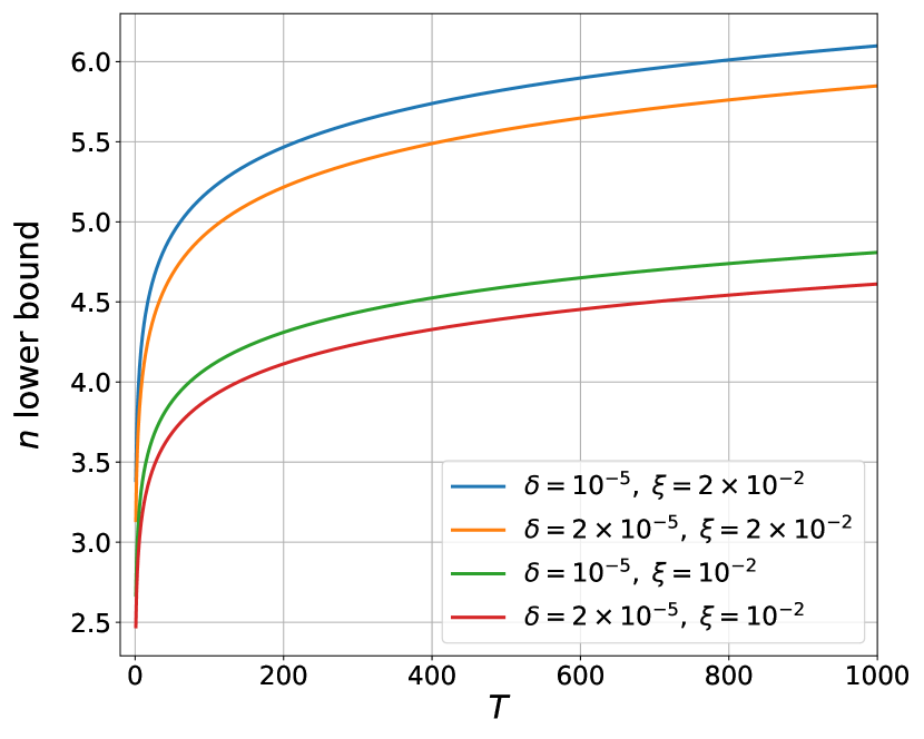
This is another impossibility result derived from our information theoretic approach, it says that for given δ𝛿\delta, ξ𝜉\xi and T𝑇T, it is impossible to use less overhead than what is given by the lower bound above. Figure 8 shows numerical values of this lower bound plotted as a function of T𝑇T for relevant values of δ𝛿\delta and ξ𝜉\xi for fault-tolerant memory.

Refer to caption
Figure 8: The error correction overhead lower bound plotted for two different values of δ𝛿\delta and ξ𝜉\xi as a function of the number of time intervals T𝑇T.

Alternatively, this result can be stated as an upper bound of the relaxation time T𝑇T

TlogΔ(δ)log(1(4ξ4ξ2)n).𝑇Δ𝛿1superscript4𝜉4superscript𝜉2𝑛T\leq\frac{\log\Delta(\delta)}{\log(1-(4\xi-4\xi^{2})^{n})}. (52)

At fixed ξ𝜉\xi and δ𝛿\delta, when n𝑛n goes to infinity, this upper bound can be approximated using a Taylor series expansion and is asymptotically equivalent to logΔ1exp(nlog(1/(4ξ4ξ2)))superscriptΔ1𝑛14𝜉4superscript𝜉2\log\Delta^{-1}\exp(n\log(1/(4\xi-4\xi^{2}))). Relaxation time upper bound grows exponentially with system size n𝑛n, at sufficiently big n𝑛n, there exists C1(δ)>0subscript𝐶1𝛿0C_{1}(\delta)>0 such that

TC1(δ)exp(nlog(14ξ4ξ2)).𝑇subscript𝐶1𝛿𝑛14𝜉4superscript𝜉2T\leq C_{1}(\delta)\exp\left(n\log\left(\frac{1}{4\xi-4\xi^{2}}\right)\right). (53)

We derive a lower bound for T𝑇T in the case of simple repetition encoding and error correction using global majority vote. In this case, an error cannot be corrected only if a catastrophic event happens where more than half of the physical memory bits are flipped by random noise before the next error correction happens, we let pesubscript𝑝𝑒p_{e} denote this probability. After Tτ𝑇𝜏T\tau, the information can be correctly decoded with a global majority vote if catastrophic events have happened an even number of times between time step 111 and T𝑇T. Since these events are independent and their distribution follows a binomial distribution. Using the relationship between odd and even binomial terms, it is easy to get the probability of correct decoding as (1+(12pe)T)/21superscript12subscript𝑝𝑒𝑇2(1+(1-2p_{e})^{T})/2. Therefore (1+(12pe)T)/2=1δ1superscript12subscript𝑝𝑒𝑇21𝛿(1+(1-2p_{e})^{T})/2=1-\delta and

T=log(12δ)log(12pe).𝑇12𝛿12subscript𝑝𝑒T=\frac{\log(1-2\delta)}{\log(1-2p_{e})}. (54)

Probability pesubscript𝑝𝑒p_{e} can be calculated as the probability of tail events in Bernoulli trials, which can be bounded with the Chernoff-Hoeffding bound (the more general form of the Chernoff bounds involving relative entropy, see Theorem 1 in [33]) as

pesubscript𝑝𝑒\displaystyle p_{e} exp(n2log(12ξ)n2log(12(1ξ)))absent𝑛212𝜉𝑛2121𝜉\displaystyle\leq\exp\left(-\frac{n}{2}\log\left(\frac{1}{2\xi}\right)-\frac{n}{2}\log\left(\frac{1}{2(1-\xi)}\right)\right)
=exp(n2log(14ξ4ξ2)).absent𝑛214𝜉4superscript𝜉2\displaystyle=\exp\left(-\frac{n}{2}\log\left(\frac{1}{4\xi-4\xi^{2}}\right)\right). (55)

Hence for sufficiently big n𝑛n, there exists C2(δ)>0subscript𝐶2𝛿0C_{2}(\delta)>0 such that

TC2(δ)exp(n2log(14ξ4ξ2)).𝑇subscript𝐶2𝛿𝑛214𝜉4superscript𝜉2T\geq C_{2}(\delta)\exp\left(\frac{n}{2}\log\left(\frac{1}{4\xi-4\xi^{2}}\right)\right). (56)

Comparing our upper bound in Inequality (53) and the lower bound in Inequality (56), our information contraction results give a nontrivial upper bound of the relaxation time T𝑇T that is asymptotically tight up to a constant factor of 222 in the exponent. Relaxation time that grows exponentially with size n𝑛n of the system is provably the best that can be achieved. Global majority vote is expensive to implement, there are local update rules such as the 2-dimensional Toom’s rule [17] that can also achieve exponential growth in relaxation time [34].

We also note that some fault-tolerant cellular automata can be stable even if the errors are correlated [15], and results similar to Proposition 2 can potentially be developed for fault-tolerant cellular automata.

VI Conclusion

In this paper, we have made contributions to the fundamental understanding of neural networks or general networks with noisy components. Information theoretic tools are shown to be essential to this study. We prove a strong data processing inequality which may find broader application and is thus interesting in its own right. The information contraction bounds given by our method improve the previous results by Evans and Schulman. Information contraction bounds are derived for both independent and weakly-correlated neuron noise models. Leveraging these results, we have shown that information contraction in noisy neural networks requires an increase in the minimum number of neurons to provide adequate noise robustness. Robust information flow favors wide and shallow networks over narrower and deeper ones, while network expressibility requirements favor the opposite. An optimal minimum network depth which gives the most neuron efficient lower bound is obtained from the balance of these two effects. Additionally, we show an application of our results to fault-tolerant cellular automata, showcasing wider applicability of our approach. This work can be readily applied to advance the understanding of information processing systems found in neuroscience, physics and electronics, where noise is naturally present.

Finally, we list some potential future directions. We have derived an SDPI for discrete channels and therefore considered binary neural networks; hence, the generalization of our SDPI results to the continuous-variable case is crucial to precise information bounds for general neural networks beyond the binary case. We have considered independent neuron noise and a special case of weakly-correlated neuron noise, more general correlated neuron noise models in noisy neural networks can potentially be studied by our Theorem 1. It may also be interesting to use Theorem 1 to derive network weight dependent SDPIs and rule-dependent relaxation time for different fault-tolerant cellular automata.

Note added. After the completion of this work, we have become aware of a recent extension [35] of Theorem 21 of Ref. [25] that can lead to our Theorem 1 via a different proof.

Appendix A Proof of Lemma 1

Let M𝑀M denote the supremum:

M=sup𝒄IRn𝒙𝒫̊n𝒄𝐇f(𝒙)𝒄𝒄𝐇g(𝒙)𝒄.𝑀subscriptsupremumfor-all𝒄IsuperscriptR𝑛for-all𝒙subscript̊𝒫𝑛superscript𝒄subscript𝐇𝑓𝒙𝒄superscript𝒄subscript𝐇𝑔𝒙𝒄M=\sup_{\begin{subarray}{c}\forall\boldsymbol{c}\in{\rm I\!R}^{n}\\ \forall\boldsymbol{x}\in\mathring{\mathcal{P}}_{n}\end{subarray}}\frac{\boldsymbol{c}^{\intercal}\mathbf{H}_{f}(\boldsymbol{x})\boldsymbol{c}}{\boldsymbol{c}^{\intercal}\mathbf{H}_{g}(\boldsymbol{x})\boldsymbol{c}}. (57)

If M𝑀M is finite, by definition, we have 𝒄IRnfor-all𝒄IsuperscriptR𝑛\forall\boldsymbol{c}\in{\rm I\!R}^{n} and 𝒙𝒫̊nfor-all𝒙subscript̊𝒫𝑛\forall\boldsymbol{x}\in\mathring{\mathcal{P}}_{n}, 𝒄[𝐇f(𝒙)M𝐇g(𝒙)]𝒄0superscript𝒄delimited-[]subscript𝐇𝑓𝒙𝑀subscript𝐇𝑔𝒙𝒄0\boldsymbol{c}^{\intercal}[\mathbf{H}_{f}(\boldsymbol{x})-M\mathbf{H}_{g}(\boldsymbol{x})]\boldsymbol{c}\leq 0. Additionally, linearity of taking the second derivatives gives 𝐇f(𝒙)M𝐇g(𝒙)=𝐇fMg(𝒙)subscript𝐇𝑓𝒙𝑀subscript𝐇𝑔𝒙subscript𝐇𝑓𝑀𝑔𝒙\mathbf{H}_{f}(\boldsymbol{x})-M\mathbf{H}_{g}(\boldsymbol{x})=\mathbf{H}_{f-Mg}(\boldsymbol{x}). The Hessian matrix 𝐇fMg(𝒙)subscript𝐇𝑓𝑀𝑔𝒙\mathbf{H}_{f-Mg}(\boldsymbol{x}) is negative semi-definite. Hence function fMg𝑓𝑀𝑔f-Mg is also a concave function on 𝒫̊nsubscript̊𝒫𝑛\mathring{\mathcal{P}}_{n}. Apply Jensen’s inequality to the concave function fMg𝑓𝑀𝑔f-Mg for d𝑑d points (𝒙1,,𝒙d)subscript𝒙1subscript𝒙𝑑(\boldsymbol{x}_{1},...,\boldsymbol{x}_{d}) on 𝒫̊nsubscript̊𝒫𝑛\mathring{\mathcal{P}}_{n} with weights (p1,,pd)subscript𝑝1subscript𝑝𝑑(p_{1},...,p_{d})

i=1dpi(fMg)(𝒙i)(fMg)(i=1dpi𝒙i).superscriptsubscript𝑖1𝑑subscript𝑝𝑖𝑓𝑀𝑔subscript𝒙𝑖𝑓𝑀𝑔superscriptsubscript𝑖1𝑑subscript𝑝𝑖subscript𝒙𝑖\sum_{i=1}^{d}p_{i}(f-Mg)(\boldsymbol{x}_{i})\leq(f-Mg)\left(\sum_{i=1}^{d}p_{i}\boldsymbol{x}_{i}\right). (58)

Rearrange the terms, we have for (𝒙1,,𝒙d)𝒫̊nd,(p1,,pd)𝒫d1formulae-sequencefor-allsubscript𝒙1subscript𝒙𝑑superscriptsubscript̊𝒫𝑛𝑑for-allsubscript𝑝1subscript𝑝𝑑subscript𝒫𝑑1\forall(\boldsymbol{x}_{1},...,\boldsymbol{x}_{d})\in\mathring{\mathcal{P}}_{n}^{d},\forall(p_{1},...,p_{d})\in\mathcal{P}_{d-1},

i=1mpif(𝒙i)f(i=1mpi𝒙i)superscriptsubscript𝑖1𝑚subscript𝑝𝑖𝑓subscript𝒙𝑖𝑓superscriptsubscript𝑖1𝑚subscript𝑝𝑖subscript𝒙𝑖absent\displaystyle\sum_{i=1}^{m}p_{i}f(\boldsymbol{x}_{i})-f(\sum_{i=1}^{m}p_{i}\boldsymbol{x}_{i})\leq (59)
M[i=1mpig(𝒙i)g(i=1mpi𝒙i)].𝑀delimited-[]superscriptsubscript𝑖1𝑚subscript𝑝𝑖𝑔subscript𝒙𝑖𝑔superscriptsubscript𝑖1𝑚subscript𝑝𝑖subscript𝒙𝑖\displaystyle M\left[\sum_{i=1}^{m}p_{i}g(\boldsymbol{x}_{i})-g(\sum_{i=1}^{m}p_{i}\boldsymbol{x}_{i})\right].

Therefore,

sup(𝒙1,,𝒙d)𝒫̊nd(p1,,pd)𝒫d1f2(𝒙1,,𝒙d;p1,,pd)g2(𝒙1,,𝒙d;p1,,pd)M.subscriptsupremumfor-allsubscript𝒙1subscript𝒙𝑑superscriptsubscript̊𝒫𝑛𝑑for-allsubscript𝑝1subscript𝑝𝑑subscript𝒫𝑑1subscript𝑓2subscript𝒙1subscript𝒙𝑑subscript𝑝1subscript𝑝𝑑subscript𝑔2subscript𝒙1subscript𝒙𝑑subscript𝑝1subscript𝑝𝑑𝑀\sup_{\begin{subarray}{c}\forall(\boldsymbol{x}_{1},...,\boldsymbol{x}_{d})\in\mathring{\mathcal{P}}_{n}^{d}\\ \forall(p_{1},...,p_{d})\in\mathcal{P}_{d-1}\end{subarray}}\frac{f_{2}(\boldsymbol{x}_{1},...,\boldsymbol{x}_{d};p_{1},...,p_{d})}{g_{2}(\boldsymbol{x}_{1},...,\boldsymbol{x}_{d};p_{1},...,p_{d})}\leq M. (60)

The above inequality trivially holds when M𝑀M is infinite. We proceed to show that the upper bound M𝑀M can be effectively attained by the supremum on the left-hand side for the equality to hold. There exists a sequence (𝒙~j)subscript~𝒙𝑗(\tilde{\boldsymbol{x}}_{j}) in 𝒫̊nsubscript̊𝒫𝑛\mathring{\mathcal{P}}_{n} such that 𝒄~IRn~𝒄IsuperscriptR𝑛\exists\tilde{\boldsymbol{c}}\in{\rm I\!R}^{n} and 𝒄~2=1subscriptnorm~𝒄21\left\|\tilde{\boldsymbol{c}}\right\|_{2}=1, limj𝒄~𝐇f(𝒙~j)𝒄~𝒄~𝐇g(𝒙~j)𝒄~=Msubscript𝑗superscript~𝒄subscript𝐇𝑓subscript~𝒙𝑗~𝒄superscript~𝒄subscript𝐇𝑔subscript~𝒙𝑗~𝒄𝑀\lim_{j\to\infty}\frac{\tilde{\boldsymbol{c}}^{\intercal}\mathbf{H}_{f}(\tilde{\boldsymbol{x}}_{j})\tilde{\boldsymbol{c}}}{\tilde{\boldsymbol{c}}^{\intercal}\mathbf{H}_{g}(\tilde{\boldsymbol{x}}_{j})\tilde{\boldsymbol{c}}}=M. Consider {𝒙1,,𝒙d}subscript𝒙1subscript𝒙𝑑\left\{\boldsymbol{x}_{1},...,\boldsymbol{x}_{d}\right\} and 𝒙i=𝒙~j+Δ𝒙isubscript𝒙𝑖subscript~𝒙𝑗Δsubscript𝒙𝑖\boldsymbol{x}_{i}=\tilde{\boldsymbol{x}}_{j}+\Delta\boldsymbol{x}_{i} with j𝑗j fixed, in the limit where all Δ𝒙iΔsubscript𝒙𝑖\Delta\boldsymbol{x}_{i} vanish: Δ𝒙i0Δsubscript𝒙𝑖0\Delta\boldsymbol{x}_{i}\to 0, we can expand f2subscript𝑓2f_{2} and g2subscript𝑔2g_{2} in their Taylor series up to the second order in Δ𝒙iΔsubscript𝒙𝑖\Delta\boldsymbol{x}_{i}

f2(𝒙1,,𝒙d;p1,,pd)=12i=1dpiΔ𝒙i𝐇f(𝒙~j)Δ𝒙isubscript𝑓2subscript𝒙1subscript𝒙𝑑subscript𝑝1subscript𝑝𝑑12superscriptsubscript𝑖1𝑑subscript𝑝𝑖Δsuperscriptsubscript𝒙𝑖subscript𝐇𝑓subscript~𝒙𝑗Δsubscript𝒙𝑖\displaystyle f_{2}(\boldsymbol{x}_{1},...,\boldsymbol{x}_{d};p_{1},...,p_{d})=\frac{1}{2}\sum_{i=1}^{d}p_{i}\Delta\boldsymbol{x}_{i}^{\intercal}\mathbf{H}_{f}(\tilde{\boldsymbol{x}}_{j})\Delta\boldsymbol{x}_{i}
12(i=1dpiΔ𝒙i)𝐇f(𝒙~j)(i=1dpiΔ𝒙i)+𝒪(Δ𝒙i3),12superscriptsuperscriptsubscript𝑖1𝑑subscript𝑝𝑖Δsubscript𝒙𝑖subscript𝐇𝑓subscript~𝒙𝑗superscriptsubscript𝑖1𝑑subscript𝑝𝑖Δsubscript𝒙𝑖𝒪superscriptnormΔsubscript𝒙𝑖3\displaystyle-\frac{1}{2}(\sum_{i=1}^{d}p_{i}\Delta\boldsymbol{x}_{i})^{\intercal}\mathbf{H}_{f}(\tilde{\boldsymbol{x}}_{j})(\sum_{i=1}^{d}p_{i}\Delta\boldsymbol{x}_{i})+\mathcal{O}(\left\|\Delta\boldsymbol{x}_{i}\right\|^{3}), (61)
g2(𝒙1,,𝒙d;p1,,pd)=12i=1dpiΔ𝒙i𝐇g(𝒙~j)Δ𝒙isubscript𝑔2subscript𝒙1subscript𝒙𝑑subscript𝑝1subscript𝑝𝑑12superscriptsubscript𝑖1𝑑subscript𝑝𝑖Δsuperscriptsubscript𝒙𝑖subscript𝐇𝑔subscript~𝒙𝑗Δsubscript𝒙𝑖\displaystyle g_{2}(\boldsymbol{x}_{1},...,\boldsymbol{x}_{d};p_{1},...,p_{d})=\frac{1}{2}\sum_{i=1}^{d}p_{i}\Delta\boldsymbol{x}_{i}^{\intercal}\mathbf{H}_{g}(\tilde{\boldsymbol{x}}_{j})\Delta\boldsymbol{x}_{i}
12(i=1dpiΔ𝒙i)𝐇g(𝒙~j)(i=1dpiΔ𝒙i)+𝒪(Δ𝒙i3).12superscriptsuperscriptsubscript𝑖1𝑑subscript𝑝𝑖Δsubscript𝒙𝑖subscript𝐇𝑔subscript~𝒙𝑗superscriptsubscript𝑖1𝑑subscript𝑝𝑖Δsubscript𝒙𝑖𝒪superscriptnormΔsubscript𝒙𝑖3\displaystyle-\frac{1}{2}(\sum_{i=1}^{d}p_{i}\Delta\boldsymbol{x}_{i})^{\intercal}\mathbf{H}_{g}(\tilde{\boldsymbol{x}}_{j})(\sum_{i=1}^{d}p_{i}\Delta\boldsymbol{x}_{i})+\mathcal{O}(\left\|\Delta\boldsymbol{x}_{i}\right\|^{3}). (62)

It is easy to verify that the zeroth order and first order terms all vanish in these expansions. Now choose Δ𝒙i=λi𝒄~Δsubscript𝒙𝑖subscript𝜆𝑖~𝒄\Delta\boldsymbol{x}_{i}=\lambda_{i}\tilde{\boldsymbol{c}} (this is obviously possible with small enough λisubscript𝜆𝑖\lambda_{i} since 𝒫̊nsubscript̊𝒫𝑛\mathring{\mathcal{P}}_{n} is an open set, geometrically we are restricting all 𝒙isubscript𝒙𝑖\boldsymbol{x}_{i} to be on the line defined by 𝒙~j+λ𝒄~subscript~𝒙𝑗𝜆~𝒄\tilde{\boldsymbol{x}}_{j}+\lambda\tilde{\boldsymbol{c}}, λIR𝜆IR\lambda\in{\rm I\!R}), then

f2(𝒙1,,𝒙d;p1,,pd)=subscript𝑓2subscript𝒙1subscript𝒙𝑑subscript𝑝1subscript𝑝𝑑absent\displaystyle f_{2}(\boldsymbol{x}_{1},...,\boldsymbol{x}_{d};p_{1},...,p_{d})=
12[i=1dpiλi2(i=1dpiλi)2]𝒄~𝐇f(𝒙~j)𝒄~+𝒪(λi3),12delimited-[]superscriptsubscript𝑖1𝑑subscript𝑝𝑖superscriptsubscript𝜆𝑖2superscriptsuperscriptsubscript𝑖1𝑑subscript𝑝𝑖subscript𝜆𝑖2superscript~𝒄subscript𝐇𝑓subscript~𝒙𝑗~𝒄𝒪superscriptsubscript𝜆𝑖3\displaystyle\frac{1}{2}\left[\sum_{i=1}^{d}p_{i}\lambda_{i}^{2}-\left(\sum_{i=1}^{d}p_{i}\lambda_{i}\right)^{2}\right]\tilde{\boldsymbol{c}}^{\intercal}\mathbf{H}_{f}(\tilde{\boldsymbol{x}}_{j})\tilde{\boldsymbol{c}}+\mathcal{O}(\lambda_{i}^{3}), (63)
g2(𝒙1,,𝒙d;p1,,pd)=subscript𝑔2subscript𝒙1subscript𝒙𝑑subscript𝑝1subscript𝑝𝑑absent\displaystyle g_{2}(\boldsymbol{x}_{1},...,\boldsymbol{x}_{d};p_{1},...,p_{d})=
12[i=1dpiλi2(i=1dpiλi)2]𝒄~𝐇g(𝒙~j)𝒄~+𝒪(λi3).12delimited-[]superscriptsubscript𝑖1𝑑subscript𝑝𝑖superscriptsubscript𝜆𝑖2superscriptsuperscriptsubscript𝑖1𝑑subscript𝑝𝑖subscript𝜆𝑖2superscript~𝒄subscript𝐇𝑔subscript~𝒙𝑗~𝒄𝒪superscriptsubscript𝜆𝑖3\displaystyle\frac{1}{2}\left[\sum_{i=1}^{d}p_{i}\lambda_{i}^{2}-\left(\sum_{i=1}^{d}p_{i}\lambda_{i}\right)^{2}\right]\tilde{\boldsymbol{c}}^{\intercal}\mathbf{H}_{g}(\tilde{\boldsymbol{x}}_{j})\tilde{\boldsymbol{c}}+\mathcal{O}(\lambda_{i}^{3}). (64)

Strict convexity of the square function xx2𝑥superscript𝑥2x\rightarrow x^{2} gives i=1dpiλi2(i=1dpiλi)2superscriptsubscript𝑖1𝑑subscript𝑝𝑖superscriptsubscript𝜆𝑖2superscriptsuperscriptsubscript𝑖1𝑑subscript𝑝𝑖subscript𝜆𝑖2\sum_{i=1}^{d}p_{i}\lambda_{i}^{2}\geq(\sum_{i=1}^{d}p_{i}\lambda_{i})^{2}, the identity is attained if and only if all the λisubscript𝜆𝑖\lambda_{i} are equal or (p1,,pd)subscript𝑝1subscript𝑝𝑑(p_{1},...,p_{d}) being a one-hot weight vector. It suffices to choose the values of λisubscript𝜆𝑖\lambda_{i} that are different from each other and pi=1/dsubscript𝑝𝑖1𝑑p_{i}=1/d for example, in the limit where ifor-all𝑖\forall i, λi0subscript𝜆𝑖0\lambda_{i}\to 0. The ratio f2/g2subscript𝑓2subscript𝑔2f_{2}/g_{2} tends to 𝒄~𝐇f(𝒙~j)𝒄~/𝒄~𝐇g(𝒙~j)𝒄~superscript~𝒄subscript𝐇𝑓subscript~𝒙𝑗~𝒄superscript~𝒄subscript𝐇𝑔subscript~𝒙𝑗~𝒄{\tilde{\boldsymbol{c}}^{\intercal}\mathbf{H}_{f}(\tilde{\boldsymbol{x}}_{j})\tilde{\boldsymbol{c}}}/{\tilde{\boldsymbol{c}}^{\intercal}\mathbf{H}_{g}(\tilde{\boldsymbol{x}}_{j})\tilde{\boldsymbol{c}}}. Now, let j𝑗j go to infinity, since the two limiting operations are independent from each other, we have a sequence of (𝒙1,,𝒙d)𝒫̊ndsubscript𝒙1subscript𝒙𝑑superscriptsubscript̊𝒫𝑛𝑑(\boldsymbol{x}_{1},...,\boldsymbol{x}_{d})\in\mathring{\mathcal{P}}_{n}^{d} and (p1,,pd)𝒫d1subscript𝑝1subscript𝑝𝑑subscript𝒫𝑑1(p_{1},...,p_{d})\in\mathcal{P}_{d-1} such that the ratio f2/g2subscript𝑓2subscript𝑔2f_{2}/g_{2} tends to M𝑀M. We have previously proven that M𝑀M is also an upper bound, hence

sup(𝒙1,,𝒙d)𝒫̊nd(p1,,pd)𝒫d1f2(𝒙1,,𝒙d;p1,,pd)g2(𝒙1,,𝒙d;p1,,pd)=M.subscriptsupremumfor-allsubscript𝒙1subscript𝒙𝑑superscriptsubscript̊𝒫𝑛𝑑for-allsubscript𝑝1subscript𝑝𝑑subscript𝒫𝑑1subscript𝑓2subscript𝒙1subscript𝒙𝑑subscript𝑝1subscript𝑝𝑑subscript𝑔2subscript𝒙1subscript𝒙𝑑subscript𝑝1subscript𝑝𝑑𝑀\sup_{\begin{subarray}{c}\forall(\boldsymbol{x}_{1},...,\boldsymbol{x}_{d})\in\mathring{\mathcal{P}}_{n}^{d}\\ \forall(p_{1},...,p_{d})\in\mathcal{P}_{d-1}\end{subarray}}\frac{f_{2}(\boldsymbol{x}_{1},...,\boldsymbol{x}_{d};p_{1},...,p_{d})}{g_{2}(\boldsymbol{x}_{1},...,\boldsymbol{x}_{d};p_{1},...,p_{d})}=M. (65)

This completes the proof of Lemma 1.

Appendix B More details of proof of Theorem 1

In this Appendix we give additional details that were omitted in the proof of Theorem 1. The matrix form of 𝐇f(𝒑)subscript𝐇𝑓𝒑\mathbf{H}_{f}(\boldsymbol{p}) is

{strip}
𝐇f(𝒑)=(j=1m(a1,jan,j)2i=1npiai,jj=1m(a1,jan,j)(a2,jan,j)i=1npiai,jj=1m(a1,jan,j)(an1,jan,j)i=1npiai,jj=1m(a2,jan,j)(a1,jan,j)i=1npiai,jj=1m(a2,jan,j)2i=1npiai,jj=1m(an1,jan,j)(a1,jan,j)i=1npiai,jj=1m(an1,jan,j)2i=1npiai,j).subscript𝐇𝑓𝒑matrixsuperscriptsubscript𝑗1𝑚superscriptsubscript𝑎1𝑗subscript𝑎𝑛𝑗2superscriptsubscript𝑖1𝑛subscript𝑝𝑖subscript𝑎𝑖𝑗superscriptsubscript𝑗1𝑚subscript𝑎1𝑗subscript𝑎𝑛𝑗subscript𝑎2𝑗subscript𝑎𝑛𝑗superscriptsubscript𝑖1𝑛subscript𝑝𝑖subscript𝑎𝑖𝑗superscriptsubscript𝑗1𝑚subscript𝑎1𝑗subscript𝑎𝑛𝑗subscript𝑎𝑛1𝑗subscript𝑎𝑛𝑗superscriptsubscript𝑖1𝑛subscript𝑝𝑖subscript𝑎𝑖𝑗superscriptsubscript𝑗1𝑚subscript𝑎2𝑗subscript𝑎𝑛𝑗subscript𝑎1𝑗subscript𝑎𝑛𝑗superscriptsubscript𝑖1𝑛subscript𝑝𝑖subscript𝑎𝑖𝑗superscriptsubscript𝑗1𝑚superscriptsubscript𝑎2𝑗subscript𝑎𝑛𝑗2superscriptsubscript𝑖1𝑛subscript𝑝𝑖subscript𝑎𝑖𝑗superscriptsubscript𝑗1𝑚subscript𝑎𝑛1𝑗subscript𝑎𝑛𝑗subscript𝑎1𝑗subscript𝑎𝑛𝑗superscriptsubscript𝑖1𝑛subscript𝑝𝑖subscript𝑎𝑖𝑗superscriptsubscript𝑗1𝑚superscriptsubscript𝑎𝑛1𝑗subscript𝑎𝑛𝑗2superscriptsubscript𝑖1𝑛subscript𝑝𝑖subscript𝑎𝑖𝑗\mathbf{H}_{f}(\boldsymbol{p})=-\begin{pmatrix}\displaystyle\sum_{j=1}^{m}\frac{(a_{1,j}-a_{n,j})^{2}}{\sum_{i=1}^{n}p_{i}a_{i,j}}&\displaystyle\sum_{j=1}^{m}\frac{(a_{1,j}-a_{n,j})(a_{2,j}-a_{n,j})}{\sum_{i=1}^{n}p_{i}a_{i,j}}&\dots&\displaystyle\sum_{j=1}^{m}\frac{(a_{1,j}-a_{n,j})(a_{n-1,j}-a_{n,j})}{\sum_{i=1}^{n}p_{i}a_{i,j}}\\ \displaystyle\sum_{j=1}^{m}\frac{(a_{2,j}-a_{n,j})(a_{1,j}-a_{n,j})}{\sum_{i=1}^{n}p_{i}a_{i,j}}&\displaystyle\sum_{j=1}^{m}\frac{(a_{2,j}-a_{n,j})^{2}}{\sum_{i=1}^{n}p_{i}a_{i,j}}&\ddots&\vdots\\ \vdots&\ddots&\ddots&\vdots\\ \displaystyle\sum_{j=1}^{m}\frac{(a_{n-1,j}-a_{n,j})(a_{1,j}-a_{n,j})}{\sum_{i=1}^{n}p_{i}a_{i,j}}&\dots&\dots&\displaystyle\sum_{j=1}^{m}\frac{(a_{n-1,j}-a_{n,j})^{2}}{\sum_{i=1}^{n}p_{i}a_{i,j}}\end{pmatrix}. (66)

In order to obtain Equation (20), we used the identity

{strip}
j=1mpsat,j+ptas,jps+pt=j=1mpspt(as,jat,j)2(ps+pt)i=1n+1piai,j+j=1m[(ps+pt)as,jat,ji=1n+1piai,j+us,utpspuat,jau,j+ptpuas,jau,j(ps+pt)i=1n+1piai,j].superscriptsubscript𝑗1𝑚subscript𝑝𝑠subscript𝑎𝑡𝑗subscript𝑝𝑡subscript𝑎𝑠𝑗subscript𝑝𝑠subscript𝑝𝑡superscriptsubscript𝑗1𝑚subscript𝑝𝑠subscript𝑝𝑡superscriptsubscript𝑎𝑠𝑗subscript𝑎𝑡𝑗2subscript𝑝𝑠subscript𝑝𝑡superscriptsubscript𝑖1𝑛1subscript𝑝𝑖subscript𝑎𝑖𝑗superscriptsubscript𝑗1𝑚delimited-[]subscript𝑝𝑠subscript𝑝𝑡subscript𝑎𝑠𝑗subscript𝑎𝑡𝑗superscriptsubscript𝑖1𝑛1subscript𝑝𝑖subscript𝑎𝑖𝑗subscriptformulae-sequence𝑢𝑠𝑢𝑡subscript𝑝𝑠subscript𝑝𝑢subscript𝑎𝑡𝑗subscript𝑎𝑢𝑗subscript𝑝𝑡subscript𝑝𝑢subscript𝑎𝑠𝑗subscript𝑎𝑢𝑗subscript𝑝𝑠subscript𝑝𝑡superscriptsubscript𝑖1𝑛1subscript𝑝𝑖subscript𝑎𝑖𝑗\displaystyle\sum_{j=1}^{m}\frac{p_{s}a_{t,j}+p_{t}a_{s,j}}{p_{s}+p_{t}}=\sum_{j=1}^{m}\frac{p_{s}p_{t}(a_{s,j}-a_{t,j})^{2}}{(p_{s}+p_{t})\sum_{i=1}^{n+1}p_{i}a_{i,j}}+\sum_{j=1}^{m}\left[\frac{(p_{s}+p_{t})a_{s,j}a_{t,j}}{\sum_{i=1}^{n+1}p_{i}a_{i,j}}+\frac{\sum_{u\neq s,u\neq t}p_{s}p_{u}a_{t,j}a_{u,j}+p_{t}p_{u}a_{s,j}a_{u,j}}{(p_{s}+p_{t})\sum_{i=1}^{n+1}p_{i}a_{i,j}}\right]. (67)

The full expression of Qg(𝒄)subscript𝑄𝑔𝒄Q_{g}(\boldsymbol{c}) is then:

{strip}
Qg(𝒄)subscript𝑄𝑔𝒄\displaystyle Q_{g}(\boldsymbol{c}) =s=1n(cs2+tscsct)j=1m(as,jan+1,j)2i=1n+1piai,j1s<tncsctj=1m(as,jat,j)2i=1n+1piai,jabsentsuperscriptsubscript𝑠1𝑛superscriptsubscript𝑐𝑠2subscript𝑡𝑠subscript𝑐𝑠subscript𝑐𝑡superscriptsubscript𝑗1𝑚superscriptsubscript𝑎𝑠𝑗subscript𝑎𝑛1𝑗2superscriptsubscript𝑖1𝑛1subscript𝑝𝑖subscript𝑎𝑖𝑗subscript1𝑠𝑡𝑛subscript𝑐𝑠subscript𝑐𝑡superscriptsubscript𝑗1𝑚superscriptsubscript𝑎𝑠𝑗subscript𝑎𝑡𝑗2superscriptsubscript𝑖1𝑛1subscript𝑝𝑖subscript𝑎𝑖𝑗\displaystyle=\sum_{s=1}^{n}\left(c_{s}^{2}+\sum_{t\neq s}c_{s}c_{t}\right)\sum_{j=1}^{m}\frac{(a_{s,j}-a_{n+1,j})^{2}}{\sum_{i=1}^{n+1}p_{i}a_{i,j}}-\sum_{1\leq s<t\leq n}c_{s}c_{t}\sum_{j=1}^{m}\frac{(a_{s,j}-a_{t,j})^{2}}{\sum_{i=1}^{n+1}p_{i}a_{i,j}}
+s=1n(cs2+tscsct)j=1m[(ps+pn+1)2as,jan+1,jpspn+1i=1n+1piai,j+us,un+1pspuan+1,jau,j+pn+1puas,jau,jpspn+1i=1n+1piai,j]superscriptsubscript𝑠1𝑛superscriptsubscript𝑐𝑠2subscript𝑡𝑠subscript𝑐𝑠subscript𝑐𝑡superscriptsubscript𝑗1𝑚delimited-[]superscriptsubscript𝑝𝑠subscript𝑝𝑛12subscript𝑎𝑠𝑗subscript𝑎𝑛1𝑗subscript𝑝𝑠subscript𝑝𝑛1superscriptsubscript𝑖1𝑛1subscript𝑝𝑖subscript𝑎𝑖𝑗subscriptformulae-sequence𝑢𝑠𝑢𝑛1subscript𝑝𝑠subscript𝑝𝑢subscript𝑎𝑛1𝑗subscript𝑎𝑢𝑗subscript𝑝𝑛1subscript𝑝𝑢subscript𝑎𝑠𝑗subscript𝑎𝑢𝑗subscript𝑝𝑠subscript𝑝𝑛1superscriptsubscript𝑖1𝑛1subscript𝑝𝑖subscript𝑎𝑖𝑗\displaystyle\;+\sum_{s=1}^{n}\left(c_{s}^{2}+\sum_{t\neq s}c_{s}c_{t}\right)\sum_{j=1}^{m}\left[\frac{(p_{s}+p_{n+1})^{2}a_{s,j}a_{n+1,j}}{p_{s}p_{n+1}\sum_{i=1}^{n+1}p_{i}a_{i,j}}+\frac{\sum_{u\neq s,u\neq n+1}p_{s}p_{u}a_{n+1,j}a_{u,j}+p_{n+1}p_{u}a_{s,j}a_{u,j}}{p_{s}p_{n+1}\sum_{i=1}^{n+1}p_{i}a_{i,j}}\right]
1s<tncsctj=1m[(ps+pt)2as,jat,jpspti=1n+1piai,j+us,utpspuat,jau,j+ptpuas,jau,jpspti=1n+1piai,j].subscript1𝑠𝑡𝑛subscript𝑐𝑠subscript𝑐𝑡superscriptsubscript𝑗1𝑚delimited-[]superscriptsubscript𝑝𝑠subscript𝑝𝑡2subscript𝑎𝑠𝑗subscript𝑎𝑡𝑗subscript𝑝𝑠subscript𝑝𝑡superscriptsubscript𝑖1𝑛1subscript𝑝𝑖subscript𝑎𝑖𝑗subscriptformulae-sequence𝑢𝑠𝑢𝑡subscript𝑝𝑠subscript𝑝𝑢subscript𝑎𝑡𝑗subscript𝑎𝑢𝑗subscript𝑝𝑡subscript𝑝𝑢subscript𝑎𝑠𝑗subscript𝑎𝑢𝑗subscript𝑝𝑠subscript𝑝𝑡superscriptsubscript𝑖1𝑛1subscript𝑝𝑖subscript𝑎𝑖𝑗\displaystyle\;-\sum_{1\leq s<t\leq n}c_{s}c_{t}\sum_{j=1}^{m}\left[\frac{(p_{s}+p_{t})^{2}a_{s,j}a_{t,j}}{p_{s}p_{t}\sum_{i=1}^{n+1}p_{i}a_{i,j}}+\frac{\sum_{u\neq s,u\neq t}p_{s}p_{u}a_{t,j}a_{u,j}+p_{t}p_{u}a_{s,j}a_{u,j}}{p_{s}p_{t}\sum_{i=1}^{n+1}p_{i}a_{i,j}}\right]. (68)

The full expression of Qf(𝒄)subscript𝑄𝑓𝒄Q_{f}(\boldsymbol{c}) is:

{strip}
Qf(𝒄)subscript𝑄𝑓𝒄\displaystyle Q_{f}(\boldsymbol{c}) =s=1ncs2j=1m(as,jan+1,j)2i=1n+1piai,j+1s<tncsctj=1m2(as,jan+1,j)(at,jan+1,j)i=1n+1piai,jabsentsuperscriptsubscript𝑠1𝑛superscriptsubscript𝑐𝑠2superscriptsubscript𝑗1𝑚superscriptsubscript𝑎𝑠𝑗subscript𝑎𝑛1𝑗2superscriptsubscript𝑖1𝑛1subscript𝑝𝑖subscript𝑎𝑖𝑗subscript1𝑠𝑡𝑛subscript𝑐𝑠subscript𝑐𝑡superscriptsubscript𝑗1𝑚2subscript𝑎𝑠𝑗subscript𝑎𝑛1𝑗subscript𝑎𝑡𝑗subscript𝑎𝑛1𝑗superscriptsubscript𝑖1𝑛1subscript𝑝𝑖subscript𝑎𝑖𝑗\displaystyle=\sum_{s=1}^{n}c_{s}^{2}\sum_{j=1}^{m}\frac{(a_{s,j}-a_{n+1,j})^{2}}{\sum_{i=1}^{n+1}p_{i}a_{i,j}}+\sum_{1\leq s<t\leq n}c_{s}c_{t}\sum_{j=1}^{m}\frac{2(a_{s,j}-a_{n+1,j})(a_{t,j}-a_{n+1,j})}{\sum_{i=1}^{n+1}p_{i}a_{i,j}}
=s=1ncs2j=1m(as,jan+1,j)2i=1n+1piai,j+1s<tncsctj=1m(as,jan+1,j)2+(at,jan+1,j)2(as,jat,j)2i=1n+1piai,jabsentsuperscriptsubscript𝑠1𝑛superscriptsubscript𝑐𝑠2superscriptsubscript𝑗1𝑚superscriptsubscript𝑎𝑠𝑗subscript𝑎𝑛1𝑗2superscriptsubscript𝑖1𝑛1subscript𝑝𝑖subscript𝑎𝑖𝑗subscript1𝑠𝑡𝑛subscript𝑐𝑠subscript𝑐𝑡superscriptsubscript𝑗1𝑚superscriptsubscript𝑎𝑠𝑗subscript𝑎𝑛1𝑗2superscriptsubscript𝑎𝑡𝑗subscript𝑎𝑛1𝑗2superscriptsubscript𝑎𝑠𝑗subscript𝑎𝑡𝑗2superscriptsubscript𝑖1𝑛1subscript𝑝𝑖subscript𝑎𝑖𝑗\displaystyle=\sum_{s=1}^{n}c_{s}^{2}\sum_{j=1}^{m}\frac{(a_{s,j}-a_{n+1,j})^{2}}{\sum_{i=1}^{n+1}p_{i}a_{i,j}}+\sum_{1\leq s<t\leq n}c_{s}c_{t}\sum_{j=1}^{m}\frac{(a_{s,j}-a_{n+1,j})^{2}+(a_{t,j}-a_{n+1,j})^{2}-(a_{s,j}-a_{t,j})^{2}}{\sum_{i=1}^{n+1}p_{i}a_{i,j}}
=s=1n(cs2+tscsct)j=1m(as,jan+1,j)2i=1n+1piai,j1s<tncsctj=1m(as,jat,j)2i=1n+1piai,j.absentsuperscriptsubscript𝑠1𝑛superscriptsubscript𝑐𝑠2subscript𝑡𝑠subscript𝑐𝑠subscript𝑐𝑡superscriptsubscript𝑗1𝑚superscriptsubscript𝑎𝑠𝑗subscript𝑎𝑛1𝑗2superscriptsubscript𝑖1𝑛1subscript𝑝𝑖subscript𝑎𝑖𝑗subscript1𝑠𝑡𝑛subscript𝑐𝑠subscript𝑐𝑡superscriptsubscript𝑗1𝑚superscriptsubscript𝑎𝑠𝑗subscript𝑎𝑡𝑗2superscriptsubscript𝑖1𝑛1subscript𝑝𝑖subscript𝑎𝑖𝑗\displaystyle=\sum_{s=1}^{n}\left(c_{s}^{2}+\sum_{t\neq s}c_{s}c_{t}\right)\sum_{j=1}^{m}\frac{(a_{s,j}-a_{n+1,j})^{2}}{\sum_{i=1}^{n+1}p_{i}a_{i,j}}-\sum_{1\leq s<t\leq n}c_{s}c_{t}\sum_{j=1}^{m}\frac{(a_{s,j}-a_{t,j})^{2}}{\sum_{i=1}^{n+1}p_{i}a_{i,j}}. (69)

The full derivations of Qs,t(𝒄)subscript𝑄𝑠𝑡𝒄Q_{s,t}(\boldsymbol{c}) and Qs,n+1(𝒄)subscript𝑄𝑠𝑛1𝒄Q_{s,n+1}(\boldsymbol{c}) are:

{strip}
Qs,t(𝒄)subscript𝑄𝑠𝑡𝒄\displaystyle Q_{s,t}(\boldsymbol{c}) =ptps(cs2+uscscu)+pspt(ct2+utctcu)(2+pspt+ptps)csctpsptus,utcuctptpsus,utcucsabsentsubscript𝑝𝑡subscript𝑝𝑠superscriptsubscript𝑐𝑠2subscript𝑢𝑠subscript𝑐𝑠subscript𝑐𝑢subscript𝑝𝑠subscript𝑝𝑡superscriptsubscript𝑐𝑡2subscript𝑢𝑡subscript𝑐𝑡subscript𝑐𝑢2subscript𝑝𝑠subscript𝑝𝑡subscript𝑝𝑡subscript𝑝𝑠subscript𝑐𝑠subscript𝑐𝑡subscript𝑝𝑠subscript𝑝𝑡subscriptformulae-sequence𝑢𝑠𝑢𝑡subscript𝑐𝑢subscript𝑐𝑡subscript𝑝𝑡subscript𝑝𝑠subscriptformulae-sequence𝑢𝑠𝑢𝑡subscript𝑐𝑢subscript𝑐𝑠\displaystyle=\frac{p_{t}}{p_{s}}\left(c_{s}^{2}+\sum_{u\neq s}c_{s}c_{u}\right)+\frac{p_{s}}{p_{t}}\left(c_{t}^{2}+\sum_{u\neq t}c_{t}c_{u}\right)-\left(2+\frac{p_{s}}{p_{t}}+\frac{p_{t}}{p_{s}}\right)c_{s}c_{t}-\frac{p_{s}}{p_{t}}\sum_{u\neq s,u\neq t}c_{u}c_{t}-\frac{p_{t}}{p_{s}}\sum_{u\neq s,u\neq t}c_{u}c_{s}
=ptpscs2+psptct22csctabsentsubscript𝑝𝑡subscript𝑝𝑠superscriptsubscript𝑐𝑠2subscript𝑝𝑠subscript𝑝𝑡superscriptsubscript𝑐𝑡22subscript𝑐𝑠subscript𝑐𝑡\displaystyle=\frac{p_{t}}{p_{s}}c_{s}^{2}+\frac{p_{s}}{p_{t}}c_{t}^{2}-2c_{s}c_{t}
=(ptpscspsptct)2,absentsuperscriptsubscript𝑝𝑡subscript𝑝𝑠subscript𝑐𝑠subscript𝑝𝑠subscript𝑝𝑡subscript𝑐𝑡2\displaystyle=\left(\sqrt{\frac{p_{t}}{p_{s}}}c_{s}-\sqrt{\frac{p_{s}}{p_{t}}}c_{t}\right)^{2}, (70)
Qs,n+1(𝒄)subscript𝑄𝑠𝑛1𝒄\displaystyle Q_{s,n+1}(\boldsymbol{c}) =(cs2+tscsct)(pspn+1+pn+1ps+2)+pspn+1us,tscuct+pspn+1tscsctpn+1ps(s>tcsct+s<tcsct)absentsuperscriptsubscript𝑐𝑠2subscript𝑡𝑠subscript𝑐𝑠subscript𝑐𝑡subscript𝑝𝑠subscript𝑝𝑛1subscript𝑝𝑛1subscript𝑝𝑠2subscript𝑝𝑠subscript𝑝𝑛1subscriptformulae-sequence𝑢𝑠𝑡𝑠subscript𝑐𝑢subscript𝑐𝑡subscript𝑝𝑠subscript𝑝𝑛1subscript𝑡𝑠subscript𝑐𝑠subscript𝑐𝑡subscript𝑝𝑛1subscript𝑝𝑠subscript𝑠𝑡subscript𝑐𝑠subscript𝑐𝑡subscript𝑠𝑡subscript𝑐𝑠subscript𝑐𝑡\displaystyle=\left(c_{s}^{2}+\sum_{t\neq s}c_{s}c_{t}\right)\left(\frac{p_{s}}{p_{n+1}}+\frac{p_{n+1}}{p_{s}}+2\right)+\frac{p_{s}}{p_{n+1}}\sum_{u\neq s,t\neq s}c_{u}c_{t}+\frac{p_{s}}{p_{n+1}}\sum_{t\neq s}c_{s}c_{t}-\frac{p_{n+1}}{p_{s}}\left(\sum_{s>t}c_{s}c_{t}+\sum_{s<t}c_{s}c_{t}\right)
=[cs(pspn+1+pn+1ps)+tspspn+1ct]2.absentsuperscriptdelimited-[]subscript𝑐𝑠subscript𝑝𝑠subscript𝑝𝑛1subscript𝑝𝑛1subscript𝑝𝑠subscript𝑡𝑠subscript𝑝𝑠subscript𝑝𝑛1subscript𝑐𝑡2\displaystyle=\left[c_{s}\left(\sqrt{\frac{p_{s}}{p_{n+1}}}+\sqrt{\frac{p_{n+1}}{p_{s}}}\right)+\sum_{t\neq s}\sqrt{\frac{p_{s}}{p_{n+1}}}c_{t}\right]^{2}. (71)

Acknowledgment

The work of Q. Zhuang was supported by Defense Advanced Research Projects Agency (DARPA) under Young Faculty Award (YFA) Grant No. N660012014029 and Craig M. Berge Dean’s Faculty Fellowship of University of Arizona. C. Zhou would like to thank W. Evans and J. Guo for helpful consultations. The authors would like to thank Y. Polyanskiy for bringing Ref. [35] to our attention and pointing out its connection to our Theorem 1.

References

  • [1] X. Lin, Y. Rivenson, N. T. Yardimci, M. Veli, Y. Luo, M. Jarrahi, and A. Ozcan, “All-optical machine learning using diffractive deep neural networks,” Science, vol. 361, no. 6406, pp. 1004–1008, 2018.
  • [2] P. Yao, H. Wu, B. Gao, J. Tang, Q. Zhang, W. Zhang, J. J. Yang, and H. Qian, “Fully hardware-implemented memristor convolutional neural network,” Nature, vol. 577, no. 7792, pp. 641–646, 2020.
  • [3] Y. Shen, N. C. Harris, S. Skirlo, M. Prabhu, T. Baehr-Jones, M. Hochberg, X. Sun, S. Zhao, H. Larochelle, D. Englund et al., “Deep learning with coherent nanophotonic circuits,” Nat. Photonics, vol. 11, no. 7, p. 441, 2017.
  • [4] O. I. Rumyantsev, J. A. Lecoq, O. Hernandez, Y. Zhang, J. Savall, R. Chrapkiewicz, J. Li, H. Zeng, S. Ganguli, and M. J. Schnitzer, “Fundamental bounds on the fidelity of sensory cortical coding,” Nature, vol. 580, no. 7801, pp. 100–105, 2020.
  • [5] A. Fischer and C. Igel, “Training restricted boltzmann machines: An introduction,” Pattern Recognit., vol. 47, no. 1, pp. 25–39, 2014.
  • [6] Y. Bengio, N. Léonard, and A. Courville, “Estimating or propagating gradients through stochastic neurons for conditional computation,” arXiv:1308.3432, 2013.
  • [7] J. Von Neumann, “Probabilistic logics and the synthesis of reliable organisms from unreliable components,” Automata studies, vol. 34, pp. 43–98, 1956.
  • [8] N. Pippenger, “Reliable computation by formulas in the presence of noise,” IEEE Trans. Inf. Theory, vol. 34, no. 2, pp. 194–197, 1988.
  • [9] T. Feder, “Reliable computation by networks in the presence of noise,” IEEE Trans. Inf. Theory, vol. 35, no. 3, pp. 569–571, 1989.
  • [10] W. S. Evans and L. J. Schulman, “Signal propagation and noisy circuits,” IEEE Trans. Inf. Theory, vol. 45, no. 7, pp. 2367–2373, 1999.
  • [11] M. Anthony, “Boolean functions and artificial neural networks,” Boolean Functions, vol. 2, 2003.
  • [12] R. L. Dobrushin, “Definition of random variables by conditional distributions,” Teoriya Veroyatnostei i ee Primeneniya, vol. 15, no. 3, pp. 469–497, 1970.
  • [13] E. Erkip and T. M. Cover, “The efficiency of investment information,” IEEE Trans. Inf. Theory, vol. 44, no. 3, pp. 1026–1040, 1998.
  • [14] J. C. Duchi, M. I. Jordan, and M. J. Wainwright, “Local privacy and statistical minimax rates,” in 2013 IEEE 54th Annual Symposium on Foundations of Computer Science.   IEEE, 2013, pp. 429–438.
  • [15] P. Gács, “Reliable cellular automata with self-organization,” J. Stat. Phys., vol. 103, no. 1-2, pp. 45–267, 2001.
  • [16] L. F. Gray, “A reader’s guide to gacs’s “positive rates” paper,” J. Stat. Phys., vol. 103, no. 1-2, pp. 1–44, 2001.
  • [17] A. L. Toom, “Nonergodic multidimensional system of automata,” Problemy Peredachi Informatsii, vol. 10, no. 3, pp. 70–79, 1974.
  • [18] T. M. Liggett, Interacting particle systems.   Springer Science & Business Media, 2012, vol. 276.
  • [19] S. Wolfram, “Statistical mechanics of cellular automata,” Rev. Mod. Phys., vol. 55, no. 3, p. 601, 1983.
  • [20] G. Grinstein, C. Jayaprakash, and Y. He, “Statistical mechanics of probabilistic cellular automata,” Phys. Rev. Lett., vol. 55, no. 23, p. 2527, 1985.
  • [21] N. Y. Yao, C. Nayak, L. Balents, and M. P. Zaletel, “Classical discrete time crystals,” Nat. Phys., vol. 16, no. 4, pp. 438–447, 2020.
  • [22] R. Impagliazzo, R. Paturi, and M. E. Saks, “Size–depth tradeoffs for threshold circuits,” SIAM J. Comput., vol. 26, no. 3, pp. 693–707, 1997.
  • [23] R. Ahlswede and P. Gács, “Spreading of sets in product spaces and hypercontraction of the markov operator,” The annals of probability, pp. 925–939, 1976.
  • [24] W. S. Evans, Information theory and noisy computation.   Citeseer, 1994, vol. 94, no. 57.
  • [25] Y. Polyanskiy and Y. Wu, “Strong data-processing inequalities for channels and bayesian networks,” in Convexity and Concentration.   Springer, 2017, pp. 211–249. [Online]. Available: http://people.lids.mit.edu/yp/homepage/data/simple-IMA.pdf
  • [26] N. Semenova, X. Porte, L. Andreoli, M. Jacquot, L. Larger, and D. Brunner, “Fundamental aspects of noise in analog-hardware neural networks,” Chaos: An Interdisciplinary Journal of Nonlinear Science, vol. 29, no. 10, p. 103128, 2019.
  • [27] T. M. Cover, Elements of information theory.   John Wiley & Sons, 1999.
  • [28] H. W. Lin, M. Tegmark, and D. Rolnick, “Why does deep and cheap learning work so well?” J. Stat. Phys., vol. 168, no. 6, pp. 1223–1247, 2017.
  • [29] M. Furst, J. B. Saxe, and M. Sipser, “Parity, circuits, and the polynomial-time hierarchy,” Mathematical systems theory, vol. 17, no. 1, pp. 13–27, 1984.
  • [30] J. T. Håstad, Computational limitations for small-depth circuits.   MIT press, 1987.
  • [31] L. Chen and R. Tell, “Bootstrapping results for threshold circuits “just beyond” known lower bounds,” in Proceedings of the 51st Annual ACM SIGACT Symposium on Theory of Computing, 2019, pp. 34–41.
  • [32] A. M. Turing, “The chemical basis of morphogenesis,” Bull. Math. Biol., vol. 52, no. 1-2, pp. 153–197, 1990.
  • [33] W. Hoeffding, “Probability inequalities for sums of bounded random variables,” in The Collected Works of Wassily Hoeffding.   Springer, 1994, pp. 409–426.
  • [34] P. Berman and J. Simon, “Investigations of fault-tolerant networks of computers,” in Proceedings of the twentieth annual ACM symposium on Theory of computing, 1988, pp. 66–77.
  • [35] O. Ordentlich and Y. Polyanskiy, “Strong data processing constant is achieved by binary inputs,” arXiv preprint arXiv:2010.01987, 2020.