Split-Douglas-Rachford algorithm for composite monotone inclusions and Split-ADMM

Abstract.

In this paper we provide a generalization of the Douglas-Rachford splitting (DRS) and the primal-dual algorithm [24, 55] for solving monotone inclusions in a real Hilbert space involving a general linear operator. The proposed method allows for primal and dual non-standard metrics and activates the linear operator separately from the monotone operators appearing in the inclusion. In the simplest case when the linear operator has full range, it reduces to classical DRS. Moreover, the weak convergence of primal-dual sequences to a Kuhn-Tucker point is guaranteed, generalizing the main result in [53]. Inspired by [34], we also derive a new Split-ADMM (SADMM) by applying our method to the dual of a convex optimization problem involving a linear operator which can be expressed as the composition of two linear operators. The proposed SADMM activates one linear operator implicitly and the other one explicitly, and we recover ADMM when the latter is set as the identity. Connections and comparisons of our theoretical results with respect to the literature are provided for the main algorithm and SADMM. The flexibility and efficiency of both methods is illustrated via a numerical simulations in total variation image restoration and a sparse minimization problem.

Keywords. ADMM, convex optimization, Douglas–Rachford splitting, fixed point iterations, monotone operator theory, quasinonexpansive operators, splitting algorithms.

1. Introduction

In this paper we focus on a splitting algorithm for solving the following primal-dual monotone inclusion.

Problem 1.1.

Let $\mathcal{H}$ and $\mathcal{G}$ be real Hilbert spaces, let $A\colon\mathcal{H}\rightarrow 2^{\mathcal{H}}$ and $B\colon\mathcal{G}\rightarrow 2^{\mathcal{G}}$ be maximally monotone operators, and let $L\colon\mathcal{H}\rightarrow\mathcal{G}$ be a non-zero linear bounded operator. The problem is to find $(\hat{x},\hat{u})\in\bm{Z}$, where

$$\bm{Z}=\big{\{}{(\hat{x},\hat{u})\in\mathcal{H}\times\mathcal{G}}\leavevmode\nobreak\ \big{|}\leavevmode\nobreak\ {0\in A\hat{x}+L^{*}\hat{u},\>0\in B^{-1}\hat{u}-L\hat{x}}\big{\}}$$ (1.1)

is assumed to be non-empty.

This problem arises naturally in several problems in partial differential equations coming from mechanical problems [34, 37, 38], differential inclusions [2, 52], game theory [13], among other disciplines. The set $\bm{Z}$ is the collection of Kuhn-Tucker points [3, Problem 26.30], which is also known as extended solution set (see, e.g., [25] and [30, 53] for the case when $L=\textnormal{Id}$).

It follows from [12, Proposition 2.8] that any solution $(\hat{x},\hat{u})$ to Problem 1.1 satisfies that $\hat{x}$ is a solution to the primal inclusion

$$\text{find}\quad x\in\mathcal{H}\quad\text{such that}\quad 0\in Ax+L^{*}BLx$$ (1.2)

and $\hat{u}$ is solution to the dual inclusion

$$\text{find}\quad u\in\mathcal{G}\quad\text{such that}\quad 0\in B^{-1}u-LA^{-1}(-L^{*}u).$$ (1.3)

Conversely, if $\hat{x}$ is a solution to (1.2) then there exists $\tilde{u}$ solution to (1.3) such that $(\hat{x},\tilde{u})\in\bm{Z}$ and the dual argument also holds. In the particular case when $A=\partial f$ and $B=\partial g^{*}$, for proper convex lower semicontinuous functions $f\colon\mathcal{H}\to\left]-\infty,+\infty\right]$ and $g\colon\mathcal{G}\to\left]-\infty,+\infty\right]$, any solution $\hat{x}$ to (1.2) is a solution to the primal convex optimization problem

$$\min_{x\in\mathcal{H}}\big{(}f(x)+g(Lx)\big{)},$$ (1.4)

any solution $\hat{u}$ to (1.3) is a solution to the dual problem

$$\min_{u\in\mathcal{G}}\big{(}g^{*}(u)+f^{*}(-L^{*}u)\big{)},$$ (1.5)

and the converse holds under standard qualification conditions (see, e.g., [12]). Problems (1.4) and (1.5) model several image processing problems as image restoration and denoising [18, 21, 26, 42, 46, 50], traffic theory [11, 33, 36], among others.

In the case when $L=\textnormal{Id}$, Problem 1.1 is solved by the Douglas-Rachford splitting (DRS) [41], which is a classical algorithm inspired from a numerical method for solving linear systems appearing in discretizations of PDEs [27]. Given $z_{0}\in\mathcal{H}$ and $\tau>0$, DRS generates the sequence $(z_{n})_{n\in\mathbb{N}}\subset\mathcal{H}$ via the recurrence

$$(\forall n\in\mathbb{N})\quad z_{n+1}=J_{\tau B}(2J_{\tau A}z_{n}-z_{n})+z_{n}-J_{\tau A}z_{n},$$ (1.6)

and $z_{n}\>\rightharpoonup\>\hat{z}$ for some $\hat{z}\in\mathcal{H}$ such that $J_{\tau A}\hat{z}$ is a zero of $A+B$ [41, Theorem 1], where we denote the resolvent of $M\colon\mathcal{H}\to 2^{\mathcal{H}}$ by $J_{M}=(\textnormal{Id}+M)^{-1}$. Under additional assumptions, such as weak lower semicontinuity of $J_{\tau A}$ or maximal monotonicity of $A+B$, the weak convergence of the shadow sequence $(J_{\tau A}{z_{n}})_{n\in\mathbb{N}}$ to a zero of $A+B$ is guaranteed in [41, Theorem 1]. More than thirty years later, the weak convergence of the shadow sequence to a solution is proved in [53] without any further assumption.

In the general case when $L\neq\textnormal{Id}$, a drawback of DRS is that the maximal monotonicity of $L^{*}BL$ is needed in order to ensure the weak convergence of $(z_{n})_{n\in\mathbb{N}}$ and the computation of its resolvent at each iteration usually leads to sub-iterations, at exception of very particular cases. Several algorithms in the literature including [4, 5, 6, 12, 14, 55] split the influence of the linear operator $L$ from the monotone operators, avoiding sub-iterations. In particular, we highlight the primal-dual splitting (PDS) proposed in [55], which generates a sequence in $\mathcal{H}\times\mathcal{G}$ via the recurrence

$$(\forall n\in\mathbb{N})\quad\begin{array}[]{l}\left\lfloor\begin{array}[]{l}{x}_{n+1}=J_{\tau A}({x}_{n}-\tau L^{*}{v}_{n})\\ {v}_{n+1}=J_{\sigma B^{-1}}({v}_{n}+\sigma L(2{x}_{n+1}-{x}_{n})),\end{array}\right.\end{array}$$ (1.7)

for some initial point $(x_{0},v_{0})\in\mathcal{H}\times\mathcal{G}$ and strictly positive step-sizes satisfying $\tau\sigma\|L\|^{2}<1$.

In the context of convex optimization, it is well known that DRS applied to (1.5) leads to the alternating direction method of multipliers (ADMM) [34, 35, 37], whose first step needs sub-iterations in general. This drawback is overcome by the splitting methods proposed in [4, 5, 6, 14, 19, 40, 44]. In particular, the algorithm proposed in [19] coincides with PDS in (1.7) in the optimization setting and its convergence is guaranteed if $\tau\sigma\|L\|^{2}<1$. In [24], the convergence of the sequences generated by (1.7) with step-sizes satisfying the limit condition $\tau\sigma\|L\|^{2}=1$ is studied in finite dimensions. This limit case is important because the algorithm improves its efficiency as the parameters approach the boundary (see Section 5.1), it has the advantage of tuning only one parameter, and the algorithm reduces to DRS and ADMM when $L=\textnormal{Id}$ and $\tau\sigma=1$ [19, Section 4.2]. Furthermore, a preconditioned version of (1.7) in the optimization context is proposed in [47]. In this extension, $\tau\textnormal{Id}$ and $\sigma\textnormal{Id}$ are generalized to strongly monotone self-adjoint linear operators $\varUpsilon$ and $\Sigma$, respectively, and the convergence is guaranteed under the condition $\|\Sigma^{\frac{1}{2}}LT^{\frac{1}{2}}\|<1$. A preconditioned version of (1.7) for monotone inclusions is derived in [23].

In this paper we propose and study the following splitting algorithm for solving Problem 1.1, which is a generalization of DRS when $L\neq\textnormal{Id}$ and of [23, 55].

Algorithm 1.2 (Split-Douglas-Rachford (SDR)).

In the context of Problem 1.1, let $(x_{0},u_{0})\in\mathcal{H}\times\mathcal{G}$, let $\Sigma\colon\mathcal{G}\to\mathcal{G}$ and $\varUpsilon\colon\mathcal{H}\to\mathcal{H}$ be strongly monotone self-adjoint linear operators such that $U=\varUpsilon^{-1}-L^{*}\Sigma L$ is monotone. Consider the recurrence:

$$(\forall n\in\mathbb{N})\quad\begin{array}[]{l}\left\lfloor\begin{array}[]{l}v_{n}=\Sigma(\textnormal{Id}-J_{\Sigma^{-1}B})(Lx_{n}+\Sigma^{-1}u_{n})\\ z_{n}=x_{n}-\varUpsilon L^{*}v_{n}\\ x_{n+1}=J_{\varUpsilon A}{z_{n}}\\ u_{n+1}=\Sigma L(x_{n+1}-x_{n})+v_{n}.\end{array}\right.\end{array}$$ (1.8)

Note that Algorithm 1.2 splits the influence of the linear operator from the monotone operators and, by storing $(Lx_{n})_{n\in\mathbb{N}}$, only one activation of $L$ is needed at each iteration. Moreover, in the case when $\textnormal{ran}\,L=\mathcal{G}$, we prove in Proposition 3.5 that (1.8) reduces to a preconditioned version of DRS in (1.6), in which case $J_{\varUpsilon L^{*}BL}$ has a closed formula depending on the resolvent of $B$. Other preconditioned versions of DRS are used for solving structured convex optimization problems in [6, 8, 10, 57], but they do not reduce to DRS when $L=\textnormal{Id}$. Without any further assumptions than those in Problem 1.1, we guarantee the weak convergence of the sequence $\big{(}(x_{n},u_{n})\big{)}_{n\in\mathbb{N}}$ generated by Algorithm 1.2 to a point in $\bm{Z}$, generalizing the result in [53] to the case when $L\neq\textnormal{Id}$. In the particular case when $\|\Sigma^{\frac{1}{2}}LT^{\frac{1}{2}}\|<1$, we obtain a reduction of Algorithm 1.2 to the preconditioned PDS in [47] and, when $\|\Sigma^{\frac{1}{2}}LT^{\frac{1}{2}}\|=1$, we generalize [24, Theorem 3.3] to monotone inclusions and infinite dimensions considering non-standard metrics. We also provide a numerical comparison of Algorithm 1.2 with several methods available in the literature in a total variation image reconstruction problem.

Another contribution of this manuscript is a generalization of ADMM in the convex optimization context, by applying Algorithm 1.2 to the dual problem of (1.4) when $L=KT$, for some non-trivial linear operators $T$ and $K$. This splitting, called Split-ADMM (SADMM), allows us to solve (1.4) by activating $T$ implicitly and $K$ explicitly. SADMM reduces to the classical ADMM in the case when $K=\textnormal{Id}$, $\Sigma=\sigma\textnormal{Id}$, and $\varUpsilon=\tau\textnormal{Id}$ and, in the case when $T=\textnormal{Id}$, it is a fully explicit algorithm which splits the influence of the linear operator in the first step of ADMM. We prove the weak convergence of SADMM, generalizing results in [28, 34, 35]. We also prove the equivalence between SDR and SADMM, generalizing some results in [1, 28, 34, 35, 45] to the case when $L\neq\textnormal{Id}$. In addition, we provide a version of SADMM able to deal with two linear operators as in [9]. The resulting method is a non-standard metric version of several ADMM-type algorithms in [4, 9, 51, 58] and it can be seen as an augmented Lagrangian method with a non-standard metric. We also illustrate the efficiency of SADMM by comparing its numerical performance in an academical sparse minimization example in which the matrix $L$ be factorized as $L=KT$ from its singular value decomposition (SVD). We show that the computational time may be drastically reduced by using SADMM with a suitable factorization of $L$.

The paper is organized as follows. In Section 2 we set our notation. In Section 3 we provide the proof of convergence of SDR and we connect our results with the literature. In Section 4 we derive the SADMM, we provide several theoretical results, and we compare them with the literature in convex optimization. Finally, in Section 5 we provide numerical simulations illustrating the efficiency of SDR and SADMM.

2. Notations and Preliminaries

Throughout this paper $\mathcal{H}$ and $\mathcal{G}$ are real Hilbert spaces with the scalar product ${\left\langle{{\cdot}\mid{\cdot}}\right\rangle}$ and associated norm $\|\cdot\|$. The identity operator on $\mathcal{H}$ is denoted by Id. Given a linear bounded operator $L:\mathcal{H}\to\mathcal{G}$, we denote its adjoint by $L^{*}\colon\mathcal{G}\to\mathcal{H}$, its kernel by $\ker L$, and its range by $\textnormal{ran}\,L$. The symbols $\>\rightharpoonup\>$ and $\to$ denote the weak and strong convergence, respectively. Let $D\subset\mathcal{H}$ be non-empty and let $T:D\rightarrow\mathcal{H}$. The set of fixed points of $T$ is $\textnormal{Fix}\,T=\big{\{}{x\in D}\leavevmode\nobreak\ \big{|}\leavevmode\nobreak\ {x=Tx}\big{\}}$. Let $\beta\in\left]0,+\infty\right[$. The operator $T$ is $\beta-$strongly monotone if, for every $x$ and $y$ in $D$, we have ${\left\langle{{x-y}\mid{Tx-Ty}}\right\rangle}\geq\beta\|x-y\|^{2}$, it is nonexpansive if, for every $x$ and $y$ in $D$, we have $\|Tx-Ty\|\leq\|x-y\|$, it is firmly nonexpansive if

$$(\forall x\in D)(\forall y\in D)\ \ \|Tx-Ty\|^{2}\leq\|x-y\|^{2}-\|(\textnormal{Id}-T)x-(\textnormal{Id}-T)y\|^{2},$$ (2.1)

and it is firmly quasinonexpansive if, for every $x\in D$ and $y\in\textnormal{Fix}\,T$, we have $\|Tx-y\|^{2}\leq\|x-y\|^{2}-\|Tx-x\|^{2}$. Let $A:\mathcal{H}\rightarrow 2^{\mathcal{H}}$ be a set-valued operator. The inverse of $A$ is $A^{-1}\colon u\mapsto\big{\{}{x\in\mathcal{H}}\leavevmode\nobreak\ \big{|}\leavevmode\nobreak\ {u\in Ax}\big{\}}$. The domain, range, graph, and zeros of $A$ are $\textnormal{dom}\,\,A=\big{\{}{x\in\mathcal{H}}\leavevmode\nobreak\ \big{|}\leavevmode\nobreak\ {Ax\neq\varnothing}\big{\}}$, $\textnormal{ran}\,\,A=\big{\{}{u\in\mathcal{H}}\leavevmode\nobreak\ \big{|}\leavevmode\nobreak\ {(\exists x\in\mathcal{H})\,\,u\in Ax}\big{\}}$, $\textnormal{gra}\,A=\big{\{}{(x,u)\in\mathcal{H}\times\mathcal{H}}\leavevmode\nobreak\ \big{|}\leavevmode\nobreak\ {u\in Ax}\big{\}}$, and $\textnormal{zer}A=\big{\{}{x\in\mathcal{H}}\leavevmode\nobreak\ \big{|}\leavevmode\nobreak\ {0\in Ax}\big{\}}$, respectively. The operator $A$ is monotone if, for every $(x,u)$ and $(y,v)$ in $\textnormal{gra}\,A$, we have ${\left\langle{{x-y}\mid{u-v}}\right\rangle}\geq 0$ and $A$ is maximally monotone if it is monotone and its graph is maximal in the sense of inclusions among the graphs of monotone operators. The resolvent of a maximally monotone operator $A$ is $J_{A}=(\textnormal{Id}+A)^{-1}$, which is firmly nonexpansive and satisfies $\textnormal{Fix}\,J_{A}=\textnormal{zer}A$.

For every self-adjoint monotone linear operator $U\colon\mathcal{H}\to\mathcal{H}$, we define $\|\cdot\|_{U}=\sqrt{{\left\langle{{\cdot}\mid{\cdot}}\right\rangle}_{U}}$, where ${\left\langle{{\cdot}\mid{\cdot}}\right\rangle}_{U}\colon(x,y)\to{\left\langle{{x}\mid{Uy}}\right\rangle}$ is bilinear, positive semi-definite, symmetric. For every $x$ and $y$ in $\mathcal{H}$, we have

$$\|x-y\|_{U}^{2}=\|x\|_{U}^{2}-2{\left\langle{{x}\mid{y}}\right\rangle}_{U}+\|y\|^{2}_{U}.$$ (2.2)

We denote by $\Gamma_{0}(\mathcal{H})$ the class of proper lower semicontinuous convex functions $f\colon\mathcal{H}\to\left]-\infty,+\infty\right]$. Let $f\in\Gamma_{0}(\mathcal{H})$. The Fenchel conjugate of $f$ is defined by $f^{*}\colon u\mapsto\sup_{x\in\mathcal{H}}({\left\langle{{x}\mid{u}}\right\rangle}-f(x))$, $f^{*}\in\Gamma_{0}(\mathcal{H})$, the subdifferential of $f$ is the maximally monotone operator $\partial f\colon x\mapsto\big{\{}{u\in\mathcal{H}}\leavevmode\nobreak\ \big{|}\leavevmode\nobreak\ {(\forall y\in\mathcal{H})\>\>f(x)+{\left\langle{{y-x}\mid{u}}\right\rangle}\leq f(y)}\big{\}}$, $(\partial f)^{-1}=\partial f^{*}$, and we have that $\textnormal{zer}\,\partial f$ is the set of minimizers of $f$, which is denoted by $\arg\min_{x\in\mathcal{H}}f$. Given a strongly monotone self-adjoint linear operator $\varUpsilon\colon\mathcal{H}\to\mathcal{H}$, we denote by

$$\text{\rm prox}^{\varUpsilon}_{f}\colon x\mapsto\underset{y\in\mathcal{H}}{\operatorname*{arg\,min}\,}\big{(}f(y)+\frac{1}{2}\|x-y\|_{\varUpsilon}^{2}\big{)},$$ (2.3)

and by $\text{\rm prox}_{f}=\text{\rm prox}^{\textnormal{Id}}_{f}$. We have $\text{\rm prox}^{\varUpsilon}_{f}=J_{\varUpsilon^{-1}\partial f}$ [3, Proposition 24.24(i)] and it is single valued since the objective function in (2.3) is strongly convex. Moreover, it follows from [3, Proposition 24.24] that

$$\text{\rm prox}^{\varUpsilon}_{f}=\textnormal{Id}-\varUpsilon^{-1}\,\text{\rm prox}^{\varUpsilon^{-1}}_{f^{*}}\,\varUpsilon=\varUpsilon^{-1}\,(\textnormal{Id}-\text{\rm prox}^{\varUpsilon^{-1}}_{f^{*}})\,\varUpsilon.$$ (2.4)

Given a non-empty closed convex set $C\subset\mathcal{H}$, we denote by $P_{C}$ the projection onto $C$, by $\iota_{C}\in\Gamma_{0}(\mathcal{H})$ the indicator function of $C$, which takes the value $0$ in $C$ and ${+\infty}$ otherwise, we denote by $N_{C}=\partial\iota_{C}$ the normal cone to $C$, and by $\text{\rm sri}\,C$ its strong relative interior. For further properties of monotone operators, nonexpansive mappings, and convex analysis, the reader is referred to [3].

We finish this section with a result involving monotone linear operators, which is useful for the connection of our algorithm and [47].

Proposition 2.1.

Let $\mathcal{H}$ and $\mathcal{G}$ be real Hilbert spaces, let $\varUpsilon\colon\mathcal{H}\to\mathcal{H}$ and $\Sigma\colon\mathcal{G}\to\mathcal{G}$ be strongly monotone self-adjoint linear operators, and set

$${\bm{V}}\colon\mathcal{H}\oplus\mathcal{G}\to\mathcal{H}\oplus\mathcal{G}\colon(x,u)\mapsto(\varUpsilon^{-1}x-L^{*}u,\Sigma^{-1}u-Lx).$$ (2.5)

Then, the following statements are equivalent.

1. $\varUpsilon^{-1}-L^{*}\circ\Sigma\circ L$ is monotone.

2. $\|\Sigma^{\frac{1}{2}}\circ L\circ\varUpsilon^{\frac{1}{2}}\|\leq 1$.

3. $\|\varUpsilon^{\frac{1}{2}}\circ L^{*}\circ\Sigma^{\frac{1}{2}}\|\leq 1$.

4. $\Sigma^{-1}-L\circ\varUpsilon\circ L^{*}$ is monotone.

5. For every $(x,u)\in\mathcal{H}\times\mathcal{G}$,

   $${\left\langle{{(x,u)}\mid{{\bm{V}}(x,u)}}\right\rangle}\geq\max\big{\{}\|\varUpsilon^{-1}u-L^{*}x\|_{\varUpsilon}^{2},\|\Sigma^{-1}u-Lx\|_{\Sigma}^{2}\big{\}}.$$ (2.6)

Moreover, if any of the statements above holds, ${\bm{V}}$ is $\frac{\tau\sigma}{\tau+\sigma}-$cocoercive, where $\tau>0$ and $\sigma>0$ are the strong monotonicity constants of $\varUpsilon$ and $\Sigma$, respectively.

Proof.

1$\Leftrightarrow$2: Since $\Sigma$ and $\varUpsilon$ are strongly monotone, linear, and self-adjoint, it follows from [48, Theorem p. 265] that there exists strongly monotone, linear, self-adjoint operators $\Sigma^{\frac{1}{2}}$ and $\varUpsilon^{\frac{1}{2}}$ such that $\Sigma=\Sigma^{\frac{1}{2}}\circ\Sigma^{\frac{1}{2}}$ and $\varUpsilon=\varUpsilon^{\frac{1}{2}}\circ\varUpsilon^{\frac{1}{2}}$. Moreover, $\varUpsilon$, $\Sigma$, $\varUpsilon^{\frac{1}{2}}$, and $\Sigma^{\frac{1}{2}}$ are invertible. Hence, we have

$$(\forall x\in\mathcal{H})\quad{\left\langle{{(\varUpsilon^{-1}-L^{*}\circ\Sigma\circ L)x}\mid{x}}\right\rangle} =\|\varUpsilon^{-\frac{1}{2}}x\|^{2}-\|\Sigma^{\frac{1}{2}}Lx\|^{2}$$

$$=\|\varUpsilon^{-\frac{1}{2}}x\|^{2}\left(1-\dfrac{\|\Sigma^{\frac{1}{2}}L\varUpsilon^{\frac{1}{2}}\varUpsilon^{-\frac{1}{2}}x\|^{2}}{\|\varUpsilon^{-\frac{1}{2}}x\|^{2}}\right).$$ (2.7)

Therefore, since $\varUpsilon^{-\frac{1}{2}}$ is a bijection, by denoting $y=\varUpsilon^{-\frac{1}{2}}x$, 1 yields

$$\|\Sigma^{\frac{1}{2}}\circ L\circ\varUpsilon^{\frac{1}{2}}\|=\sup_{y\in\mathcal{H}}\dfrac{\|\Sigma^{\frac{1}{2}}L\varUpsilon^{\frac{1}{2}}y\|}{\|y\|}\leq 1.$$ (2.8)

The converse clearly holds by using the norm inequality in the right hand side of (2). 2$\Leftrightarrow$3: Clear from $(\Sigma^{\frac{1}{2}}\circ L\circ\varUpsilon^{\frac{1}{2}})^{*}=\varUpsilon^{\frac{1}{2}}\circ L^{*}\circ\Sigma^{\frac{1}{2}}$. 3$\Leftrightarrow$4: It follows from 1$\Leftrightarrow$2 replacing $\Sigma$ by $\varUpsilon$ and $L$ by $L^{*}$, respectively. 1$\Leftrightarrow$5: For every $(x,u)\in\mathcal{H}\times\mathcal{G}$,

$${\left\langle{{(x,u)}\mid{{\bm{V}}(x,u)}}\right\rangle} ={\left\langle{{x}\mid{\varUpsilon^{-1}x-L^{*}u}}\right\rangle}+{\left\langle{{u}\mid{\Sigma^{-1}u-Lx}}\right\rangle}$$

$$={\left\langle{{x}\mid{(\varUpsilon^{-1}-L^{*}\Sigma L)x}}\right\rangle}+{\left\langle{{\Sigma Lx-u}\mid{Lx}}\right\rangle}+{\left\langle{{u}\mid{\Sigma^{-1}u-Lx}}\right\rangle}$$

$$={\left\langle{{x}\mid{(\varUpsilon^{-1}-L^{*}\Sigma L)x}}\right\rangle}+\|\Sigma^{-1}u-Lx\|_{\Sigma}^{2}$$ (2.9)

and, by symmetry, we analogously obtain

$${\left\langle{{(x,u)}\mid{{\bm{V}}(x,u)}}\right\rangle}={\left\langle{{u}\mid{(\Sigma^{-1}-L\varUpsilon L^{*})u}}\right\rangle}+\|\varUpsilon^{-1}x-L^{*}u\|_{\varUpsilon}^{2}.$$ (2.10)

Hence, it follows from 1 and (2) that ${\left\langle{{(x,u)}\mid{{\bm{V}}(x,u)}}\right\rangle}\geq\|\Sigma^{-1}u-Lx\|_{\Sigma}^{2}$. Since 1 is equivalent to 4, (2.10) yields ${\left\langle{{(x,u)}\mid{{\bm{V}}(x,u)}}\right\rangle}\geq\|\varUpsilon^{-1}x-L^{*}u\|_{\varUpsilon}^{2}$ and we obtain (2.6). For the converse implication it is enough to combine (2) with (2.6).

For the last assertion, note that (2.6) implies, for every $(x,u)\in\mathcal{H}\times\mathcal{G}$,

$$\begin{cases}{\left\langle{{(x,u)}\mid{{\bm{V}}(x,u)}}\right\rangle}\geq\tau\|\varUpsilon^{-1}x-L^{*}u\|^{2}\\ {\left\langle{{(x,u)}\mid{{\bm{V}}(x,u)}}\right\rangle}\geq\sigma\|\Sigma^{-1}u-Lx\|^{2}.\end{cases}$$ (2.11)

By multiplying the first equation in (2.11) by $\lambda\in\left[0,1\right]$ and the second by $(1-\lambda)$ and summing up we obtain

$${\left\langle{{(x,u)}\mid{{\bm{V}}(x,u)}}\right\rangle} \geq\lambda\tau\|\varUpsilon^{-1}x-L^{*}u\|^{2}+(1-\lambda)\sigma\|\Sigma^{-1}u-Lx\|^{2}$$

$$\geq\min\{\lambda\tau,(1-\lambda)\sigma\}\|{\bm{V}}(x,u)\|^{2}.$$ (2.12)

The result follows by noting that $\lambda\mapsto\min\{\lambda\tau,(1-\lambda)\sigma\}$ is maximized at $\lambda^{*}=\sigma/(\tau+\sigma)$. ∎

3. Convergence of Algorithm 1.2

Denote by $\bm{M}\colon\mathcal{H}\oplus\mathcal{G}\to 2^{\mathcal{H}\oplus\mathcal{G}}$ the maximally monotone operator [12, Proposition 2.7]

$$\bm{M}\colon(x,u)\mapsto(Ax+L^{*}u)\times(B^{-1}u-Lx).$$ (3.1)

For every strongly monotone self-adjoint linear operators $\varUpsilon\colon\mathcal{H}\to\mathcal{H}$ and $\Sigma\colon\mathcal{G}\to\mathcal{G}$, consider the real Hilbert space ${\bm{\mathcal{H}}}$ obtained by endowing $\mathcal{H}\times\mathcal{G}$ with the inner product ${\left\langle{{\cdot}\mid{\cdot}}\right\rangle}_{\bm{U}}$, where $\bm{U}\colon(x,u)\mapsto(\varUpsilon^{-1}x,\Sigma^{-1}u)$. More precisely,

$${\left\langle{{\cdot}\mid{\cdot}}\right\rangle}_{\bm{U}}\colon\big{(}(x,u),(y,v)\big{)}\mapsto{\left\langle{{x}\mid{\varUpsilon^{-1}y}}\right\rangle}+{\left\langle{{u}\mid{\Sigma^{-1}v}}\right\rangle},$$ (3.2)

and we denote the associated norm by $\|\cdot\|_{\bm{U}}=\sqrt{{\left\langle{{\cdot}\mid{\cdot}}\right\rangle}_{\bm{U}}}$. Observe that, since $\varUpsilon$ and $\Sigma$ are strongly monotone, the topologies of ${\bm{\mathcal{H}}}$ and $\mathcal{H}\oplus\mathcal{G}$ are equivalent.

Proposition 3.1.

In the context of Problem 1.1, let $\Sigma\colon\mathcal{G}\to\mathcal{G}$ and $\varUpsilon\colon\mathcal{H}\to\mathcal{H}$ be strongly monotone self-adjoint linear operators such that $U=\varUpsilon^{-1}-L^{*}\Sigma L$ is monotone, and define $\bm{T}:{\bm{\mathcal{H}}}\to{\bm{\mathcal{H}}}$ by

$$\bm{T}\colon\begin{pmatrix}x\\ u\end{pmatrix}\mapsto\begin{pmatrix}x_{+}\\ u_{+}\end{pmatrix}=\begin{pmatrix}J_{\varUpsilon A}\big{(}x-\varUpsilon L^{*}\Sigma(\textnormal{Id}-J_{\Sigma^{-1}B})(Lx+\Sigma^{-1}u)\big{)}\\[2.84526pt] \Sigma L(x_{+}-x)+\Sigma(\textnormal{Id}-J_{\Sigma^{-1}B})(Lx+\Sigma^{-1}u)\end{pmatrix}.$$ (3.3)

Then, the following hold:

1. For every $(x,u)\in{\bm{\mathcal{H}}}$, we have

   $$\left(\varUpsilon^{-1}(x-x_{+}),\Sigma^{-1}(u-u_{+})\right)\in\bm{M}\big{(}x_{+},u_{+}-\Sigma L(x_{+}-x)\big{)}.$$ (3.4)

2. $\textnormal{Fix}\,\bm{T}=\bm{Z}=\textnormal{zer}\bm{M}$.

3. For every $(\hat{x},\hat{u})\in\bm{Z}$ and $(x,u)\in{\bm{\mathcal{H}}}$ we have

   $$\|\bm{T}(x,u)-(\hat{x},\hat{u})\|^{2}_{\bm{U}} \leq\|(x,u)-(\hat{x},\hat{u})\|^{2}_{\bm{U}}-\|(x,u)-\bm{T}(x,u)\|^{2}_{\bm{U}}$$

   $$\hskip 99.58464pt+2{\left\langle{{u_{+}-u}\mid{L(x_{+}-x)}}\right\rangle}.$$ (3.5)

Proof.

1: From (3.3) and [3, Proposition 23.34(iii)] we obtain

$$\begin{pmatrix}x_{+}\\ u_{+}\end{pmatrix}=\bm{T}\begin{pmatrix}x\\ u\end{pmatrix}\>\> \Leftrightarrow\>\>\begin{cases}x_{+}=J_{\varUpsilon A}\big{(}x-\varUpsilon L^{*}\Sigma(\textnormal{Id}-J_{\Sigma^{-1}B})(Lx+\Sigma^{-1}u)\big{)}\\[2.84526pt] u_{+}=\Sigma L(x_{+}-x)+\Sigma(\textnormal{Id}-J_{\Sigma^{-1}B})(Lx+\Sigma^{-1}u)\end{cases}$$

$$\Leftrightarrow\>\>\begin{cases}x_{+}=J_{\varUpsilon A}\big{(}x-\varUpsilon L^{*}(u_{+}-\Sigma L(x_{+}-x))\big{)}\\[2.84526pt] u_{+}-\Sigma L(x_{+}-x)=J_{\Sigma B^{-1}}(\Sigma Lx+u)\end{cases}$$

$$\Leftrightarrow\>\>\begin{cases}\varUpsilon^{-1}(x-x_{+})-L^{*}(u_{+}-\Sigma L(x_{+}-x))\in Ax_{+}\\[2.84526pt] \Sigma^{-1}(u-u_{+})+Lx_{+}\in B^{-1}\big{(}u_{+}-\Sigma L(x_{+}-x)\big{)},\end{cases}$$ (3.6)

and the result follows from (3.1). 2: It follows from 1 and (1.1) that $\bm{T}(\hat{x},\hat{u})=(\hat{x},\hat{u})$ $\Leftrightarrow$ $(0,0)\in\bm{M}(\hat{x},\hat{u})$ $\Leftrightarrow$ $(\hat{x},\hat{u})\in\bm{Z}$. 3: Let $(\hat{x},\hat{u})\in\bm{Z}$. It follows from 2 that $(0,0)\in\bm{M}(\hat{x},\hat{u})$. Hence, 1 and the monotonicity of $\bm{M}$ in $\mathcal{H}\oplus\mathcal{G}$ yield

$$0 \leq{\left\langle{{\varUpsilon^{-1}(x-x_{+})}\mid{x_{+}-\hat{x}}}\right\rangle}+{\left\langle{{\Sigma^{-1}(u-u_{+})}\mid{u_{+}-\hat{u}+\Sigma L(x-x_{+})}}\right\rangle}$$

$$\overset{\eqref{e:defnorm}}{=}{\left\langle{{(x,u)-(x_{+},u_{+})}\mid{(x_{+},u_{+})-(\hat{x},\hat{u})}}\right\rangle}_{\bm{U}}+{\left\langle{{u-u_{+}}\mid{L(x-x_{+})}}\right\rangle}$$

$$\overset{\eqref{e:scalU}}{=}\frac{1}{2}\big{(}\|(x,u)-(\hat{x},\hat{u})\|^{2}_{\bm{U}}-\|(x,u)-(x_{+},u_{+})\|^{2}_{\bm{U}}-\|(x_{+},u_{+})-(\hat{x},\hat{u})\|^{2}_{\bm{U}}\big{)}$$

$$\hskip 142.26378pt+{\left\langle{{u-u_{+}}\mid{L(x-x_{+})}}\right\rangle}$$

and the result follows. ∎

Remark 3.2.

1. Note that (3.3) and Algorithm 1.2 yield, for every $n\in\mathbb{N}$, $(x_{n+1},u_{n+1})=(x_{n+},u_{n+})=\bm{T}(x_{n},u_{n})$. This observation and the properties of $\bm{T}$ in Proposition 3.1 are crucial for the convergence of Algorithm 1.2 in Theorem 3.3 below.

2. Proposition 3.1(3) can be written equivalently as, for every $(\hat{x},\hat{u})\in\bm{Z}$ and $(x,u)\in{\bm{\mathcal{H}}}$, $\|\bm{T}(x,u)-(\hat{x},\hat{u})\|^{2}_{\bm{U}}\leq\|(x,u)-(\hat{x},\hat{u})\|^{2}_{\bm{U}}-\|(x,u)-\bm{T}(x,u)\|^{2}_{\bm{V}}$, where $\bm{V}\colon(x,u)\mapsto(\varUpsilon^{-1}x-L^{*}u,\Sigma^{-1}u-Lx)$. Since $\varUpsilon^{-1}-L^{*}\Sigma L$ is monotone, Proposition 2.1 asserts that $\bm{V}$ is self-adjoint, linear, and cocoercive, but not strongly monotone and, thus, $\|\cdot\|^{2}_{\bm{V}}$ does not define a norm.

Theorem 3.3.

In the context of Problem 1.1, let $(x_{0},u_{0})\in\mathcal{H}\times\mathcal{G}$ and consider the sequence $\big{(}(x_{n},u_{n})\big{)}_{n\in\mathbb{N}}$ defined by the Algorithm 1.2. Then, the following assertions hold:

1. $\sum_{n\geq 1}\|x_{n+1}-x_{n}\|^{2}<{+\infty}$ and $\sum_{n\geq 1}\|u_{n+1}-u_{n}\|^{2}<{+\infty}$.

2. There exists $(\hat{x},\hat{u})\in\bm{Z}$ such that $(x_{n},u_{n})\rightharpoonup(\hat{x},\hat{u})$ in $\mathcal{H}\oplus\mathcal{G}$.

Proof.

Let ${\bm{x}}=({x},{u})\in\textnormal{Fix}\,\bm{T}$, for every $n\in\mathbb{N}$, denote by $\bm{x}_{n}=(x_{n},u_{n})$, and fix $n\geq 1$. It follows from Remark 3.2(1) that $\bm{x}_{n+1}=\bm{T}\bm{x}_{n}$ and from Proposition 3.1(2) that ${\bm{x}}\in\bm{Z}$. Therefore, Proposition 3.1(3) yields

$$\|\bm{x}_{n+1}-{\bm{x}}\|^{2}_{\bm{U}} \leq\|\bm{x}_{n}-{\bm{x}}\|^{2}_{\bm{U}}-\|\bm{x}_{n}-\bm{x}_{n+1}\|^{2}_{\bm{U}}+2{\left\langle{{u_{n+1}-u_{n}}\mid{L(x_{n+1}-x_{n})}}\right\rangle}.$$ (3.7)

Hence, we deduce from the firm non-expansiveness of $J_{\varUpsilon A}$ in $(\mathcal{H},{\left\langle{{\cdot}\mid{\cdot}}\right\rangle}_{\varUpsilon^{-1}})$ [3, Proposition 23.34(i)] and the monotonicity of $U=\varUpsilon^{-1}-L^{*}\Sigma L$ that

$${\left\langle{{u_{n+1}-u_{n}}\mid{L(x_{n+1}-x_{n})}}\right\rangle}$$

$$\hskip 42.67912pt\overset{\eqref{eq:algoSDR}}{=}{\left\langle{{\Sigma L(x_{n+1}-x_{n})+v_{n}-\Sigma L(x_{n}-x_{n-1})-v_{n-1}}\mid{L(x_{n+1}-x_{n})}}\right\rangle}$$

$$\hskip 42.67912pt={\left\langle{{x_{n+1}-x_{n}}\mid{L^{*}\Sigma L(x_{n+1}-x_{n})}}\right\rangle}+{\left\langle{{L^{*}(v_{n}-v_{n-1})}\mid{x_{n+1}-x_{n}}}\right\rangle}$$

$$\hskip 82.51282pt-{\left\langle{{\Sigma L(x_{n}-x_{n-1})}\mid{L(x_{n+1}-x_{n})}}\right\rangle}$$

$$\hskip 42.67912pt={\left\langle{{x_{n+1}-x_{n}}\mid{L^{*}\Sigma L(x_{n+1}-x_{n})}}\right\rangle}+{\left\langle{{\varUpsilon^{-1}(x_{n}-x_{n-1})}\mid{x_{n+1}-x_{n}}}\right\rangle}$$

$$\hskip 82.51282pt-{\left\langle{{(x_{n}-\varUpsilon L^{*}v_{n}-(x_{n-1}-\varUpsilon L^{*}v_{n-1}))}\mid{x_{n+1}-x_{n}}}\right\rangle}_{\varUpsilon^{-1}}$$

$$\hskip 82.51282pt-{\left\langle{{\Sigma L(x_{n}-x_{n-1})}\mid{L(x_{n+1}-x_{n})}}\right\rangle}$$

$$\hskip 42.67912pt\leq{\left\langle{{x_{n+1}-x_{n}}\mid{L^{*}\Sigma L(x_{n+1}-x_{n})}}\right\rangle}+{\left\langle{{\varUpsilon^{-1}(x_{n}-x_{n-1})}\mid{x_{n+1}-x_{n}}}\right\rangle}$$

$$\hskip 82.51282pt-\|x_{n+1}-x_{n}\|_{\varUpsilon^{-1}}^{2}-{\left\langle{{L^{*}\Sigma L(x_{n}-x_{n-1})}\mid{x_{n+1}-x_{n}}}\right\rangle}$$

$$\hskip 42.67912pt=-\|x_{n+1}-x_{n}\|^{2}_{U}+{\left\langle{{x_{n}-x_{n-1}}\mid{x_{n+1}-x_{n}}}\right\rangle}_{U}$$

$$\hskip 42.67912pt\overset{\eqref{e:scalU}}{=}-\frac{1}{2}\|x_{n+1}-x_{n}\|^{2}_{U}+\frac{1}{2}\|x_{n}-x_{n-1}\|^{2}_{U}-\frac{1}{2}\|x_{n+1}+x_{n-1}-2x_{n}\|^{2}_{U}$$

$$\hskip 42.67912pt\leq-\frac{1}{2}\|x_{n+1}-x_{n}\|^{2}_{U}+\frac{1}{2}\|x_{n}-x_{n-1}\|^{2}_{U}.$$ (3.8)

Therefore, it follows from (3.7) that

$$(\forall n\geq 1)\quad\|\bm{x}_{n+1}-{\bm{x}}\|^{2}_{\bm{U}}+\|x_{n+1}-x_{n}\|^{2}_{U}\leq\|\bm{x}_{n}-{\bm{x}}\|^{2}_{\bm{U}}+\|x_{n}-x_{n-1}\|^{2}_{U}\\ -\|\bm{x}_{n}-\bm{x}_{n+1}\|^{2}_{\bm{U}}.$$ (3.9)

Thus, [22, Lemma 3.1] asserts that

$$(\forall{\bm{x}}\in\bm{Z})\quad\big{(}\|\bm{x}_{n}-{\bm{x}}\|^{2}_{\bm{U}}+\|x_{n}-x_{n-1}\|^{2}_{U}\big{)}_{n\geq 1}\quad\text{converges},$$ (3.10)

that

$$\sum_{n\geq 1}\|\bm{x}_{n+1}-\bm{x}_{n}\|^{2}_{\bm{U}}<{+\infty},$$ (3.11)

and 1 follows from (3.2) and the strong monotonicity of $\varUpsilon^{-1}$ and $\Sigma^{-1}$ [48, p.266].

In order to prove 2, note that, from 1 and the uniform continuity of $U$, we deduce $\|x_{n}-x_{n-1}\|^{2}_{U}\to 0$. Hence, (3.10) implies that, for every ${\bm{x}}\in\bm{Z}$, $(\|\bm{x}_{n}-{\bm{x}}\|^{2}_{\bm{U}})_{n\in\mathbb{N}}$ converges. Now, let $(\overline{x},\overline{u})\in{\bm{\mathcal{H}}}$ be a weak sequential cluster point of $\big{(}(x_{n},u_{n})\big{)}_{n\in\mathbb{N}}$, say $(x_{k_{n}},u_{k_{n}})\rightharpoonup(\overline{x},\overline{u})$ in ${\bm{\mathcal{H}}}$. It is clear from (3.2) that we have $x_{k_{n}}\>\rightharpoonup\>\overline{x}$ in $\mathcal{H}$ and $u_{k_{n}}\>\rightharpoonup\>\overline{u}$ in $\mathcal{G}$ and from 1 that $x_{k_{n}+1}\>\rightharpoonup\>\overline{x}$ and $u_{k_{n}+1}\rightharpoonup\overline{u}$. Hence, since Proposition 3.1(1) yields

$$\left(\varUpsilon^{-1}(x_{k_{n}}-x_{k_{n}+1}),\Sigma^{-1}(u_{k_{n}}-u_{k_{n}+1})\right)\in\bm{M}\big{(}x_{k_{n}+1},u_{k_{n}+1}-\Sigma L(x_{k_{n}+1}-x_{k_{n}})\big{)},$$ (3.12)

we deduce from 1, the uniform continuity of $\Sigma L$, $\varUpsilon^{-1}$, and $\Sigma^{-1}$, and [3, Proposition 20.38(ii)], that $(0,0)\in\bm{M}(\overline{x},\overline{u})$. Therefore, we conclude from [3, Lemma 2.47] that there exists $\hat{\bm{x}}\in\textnormal{Fix}\,\bm{T}$ such that $\bm{x}_{n}\>\rightharpoonup\>\hat{\bm{x}}$ and the result follows from the equivalence of the topologies of ${\bm{\mathcal{H}}}$ and $\mathcal{H}\oplus\mathcal{G}$. ∎

Remark 3.4.

1. In the proof of Theorem 3.3, we can also deduce that any weak accumulation point of $((x_{n},u_{n}))_{n\in\mathbb{N}}$ is in $\bm{Z}$ by using the points in the graph of $A$ and $B$ obtained from (3.6) and [3, Proposition 26.5(i)].

2. The method can include summable errors in the computation of resolvents and linear operators, by using standard Quasi-Féjer sequences. We prefer to not include this extension for simplicity of our algorithm formulation.

3. Consider the sequences $(v_{n})_{n\in\mathbb{N}}$, $(z_{n})_{n\in\mathbb{N}}$, $(x_{n})_{n\in\mathbb{N}}$, $(u_{n})_{n\in\mathbb{N}}$ defined by Algorithm 1.2 with starting point $(x_{0},u_{0})\in\mathcal{H}\times\mathcal{G}$. It follows from (1.8) and [3, Proposition 23.34(iii)] that, for every $n\in\mathbb{N}$,

   $${v}_{n+1} =\Sigma(\textnormal{Id}-J_{\Sigma^{-1}B})(Lx_{n+1}+\Sigma^{-1}u_{n+1})$$

   $$=J_{\Sigma B^{-1}}(\Sigma Lx_{n+1}+u_{n+1})$$

   $$=J_{\Sigma B^{-1}}({v}_{n}+\Sigma L(2x_{n+1}-x_{n})),$$

   leading to

   $$(\forall n\in\mathbb{N})\quad\begin{array}[]{l}\left\lfloor\begin{array}[]{l}{x}_{n+1}=J_{\varUpsilon A}({x}_{n}-\varUpsilon L^{*}{v}_{n})\\ {v}_{n+1}=J_{\Sigma B^{-1}}({v}_{n}+\Sigma L(2{x}_{n+1}-{x}_{n})),\end{array}\right.\end{array}$$ (3.13)

   with starting point $(x_{0},\Sigma(\textnormal{Id}-J_{\Sigma^{-1}B})(Lx_{0}+\Sigma^{-1}u_{0}))\in\mathcal{H}\times\mathcal{G}$. When $\|\Sigma^{\frac{1}{2}}\circ L\circ\varUpsilon^{\frac{1}{2}}\|<1$, (3.13) is equivalent to the proximal point algorithm applied to $\bm{V}^{-1}\bm{M}$ in $(\mathcal{H}\times\mathcal{G},{\left\langle{{\cdot}\mid{\cdot}}\right\rangle}_{\bm{V}})$, where $\bm{V}\colon(x,u)\mapsto(\varUpsilon^{-1}x-L^{*}u,\Sigma^{-1}u-Lx)$ is strongly monotone in view of [47, Lemma 1]. Moreover, when $\varUpsilon=\tau\textnormal{Id}$, $\Sigma=\sigma\textnormal{Id}$, and $\sigma\tau\|L\|^{2}<1$, (3.13) coincides with the PDS in (1.7) [19, 24, 40, 55]. As stated in Remark 3.2, under our assumptions $\bm{V}$ is no longer strongly monotone and the same approach cannot be used. On the other hand, a generalization of the previous approach is provided in [55] using the forward-backward splitting in order to allow cocoercive operators in the monotone inclusion when $\bm{V}$ is strongly monotone. In the optimization context, the inclusion of cocoercive operators allows for convex differentiable functions with $\beta^{-1}-$Lipschitz gradients in the objective function and the convergence results are guaranteed under the more restrictive assumption $\sigma\tau\|L\|^{2}<1-\tau/2\beta$ [24, Theorem 3.1]. Hence, the inclusion of cocoercive operators modifies our monotonicity assumption on $U$ in Algorithm 1.2 distancing us from our main results. This leads us to consider this extension as part of further research.

4. We deduce from (3.13) and (1.8) that the primal iterates of SDR coincide with those of PDS in (3.13) and SDR includes an additional inertial step in the dual updates, more precisely,

   $$(\forall n\in\mathbb{N})\quad u_{n+1}=\Sigma L(x_{n+1}-x_{n})+v_{n}.$$ (3.14)

   Hence, it follows from Theorem 3.3(1)&(2) and the uniform continuity of $\Sigma L$ that $v_{n}\>\rightharpoonup\>\hat{u}$. As a consequence, we obtain the primal-dual weak convergence of (3.13) when $\|\Sigma^{\frac{1}{2}}\circ L\circ\varUpsilon^{\frac{1}{2}}\|\leq 1$, which generalizes [47, Theorem 1] and [24, Theorem 3.3], in the case when $\Sigma=\sigma\textnormal{Id}$ and $\varUpsilon=\tau\textnormal{Id}$, to monotone inclusions and infinite dimensions.

5. By using product space techniques, Algorithm 1.2 allows us to solve

   $$\text{find }\hat{x}\in\mathcal{H}\>\>\text{such that}\quad 0\in A\hat{x}+\sum_{i=1}^{m}L_{i}^{*}B_{i}L_{i}\hat{x},$$ (3.15)

   where, for every $i\in\{1,\ldots,m\}$, $\mathcal{G}_{i}$ is a real Hilbert space, $A\colon\mathcal{H}\to 2^{\mathcal{H}}$ and $B_{i}\colon\mathcal{G}_{i}\to 2^{\mathcal{G}_{i}}$ are maximally monotone, and $L_{i}\colon\mathcal{H}\to\mathcal{G}_{i}$ is a linear bounded operator. Indeed, by setting $\mathcal{G}=\oplus_{1\leq i\leq m}\mathcal{G}_{i}$, $B\colon(u_{i})_{1\leq i\leq m}\mapsto\times_{i=1}^{m}B_{i}u_{i}$, and $L\colon x\mapsto(L_{i}x)_{1\leq i\leq m}$, (3.15) is equivalent to (1.2). Hence, by setting $\Sigma\colon(u_{i})_{1\leq i\leq m}\mapsto(\Sigma_{i}u_{i})_{1\leq i\leq m}$, where $(\Sigma_{i})_{1\leq i\leq m}$ are strongly monotone operators, previous remark allows us to write Algorithm 1.2 as

   $$(\forall n\in\mathbb{N})\quad\begin{array}[]{l}\left\lfloor\begin{array}[]{l}{x}_{n+1}=J_{\varUpsilon A}({x}_{n}-\varUpsilon\sum_{i=1}^{m}L_{i}^{*}{v}_{i,n})\\ {v}_{1,n+1}=J_{\Sigma_{1}B_{1}^{-1}}({v}_{1,n}+\Sigma_{1}L_{1}(2{x}_{n+1}-{x}_{n}))\\ \hskip 34.14322pt\vdots\\ {v}_{m,n+1}=J_{\Sigma_{m}B_{m}^{-1}}({v}_{m,n}+\Sigma_{1}L_{m}(2{x}_{n+1}-{x}_{n})),\end{array}\right.\end{array}$$ (3.16)

   and the weak convergence of $(x_{n})_{n\in\mathbb{N}}$ to a solution to (3.15) is guaranteed by Theorem 3.3, assuming that

   $$\varUpsilon^{-1}-\sum_{i=1}^{m}L_{i}^{*}\Sigma_{i}L_{i}\quad\text{is monotone.}$$ (3.17)

   Note that (3.16) has the same structure as the algorithm in [23, Corollary 6.2] without considering cocoercive operators or relaxation steps, but the convergence is guaranteed under the weaker assumption (3.17).

6. Suppose that $\textnormal{ran}\,L^{*}=\mathcal{H}$ and that $\varUpsilon=(L^{*}\Sigma L)^{-1}$. Then, $U=\varUpsilon^{-1}-L^{*}\Sigma L=0$ and the operator ${\bm{T}}$ defined in (3.3) is firmly quasinonexpansive in ${\bm{\mathcal{H}}}$, in view of Proposition 3.1(3) and (3.9). We thus generalize [53, Corollary 3]. Observe that, in the particular case when $L=\textnormal{Id}$, we have $\varUpsilon=\Sigma^{-1}$ and the operator ${\bm{T}}$ defined in (3.3) reduces to $\bm{T}\colon(x,u)\mapsto\Phi_{A}^{\varUpsilon}(J_{\varUpsilon B}(x+\varUpsilon u)-\varUpsilon u),$ where

   $$\Phi_{A}^{\varUpsilon}\colon\mathcal{H}\mapsto\mathcal{H}\times\mathcal{H}\colon z\mapsto(J_{\varUpsilon A}z,\varUpsilon^{-1}(J_{\varUpsilon A}-\textnormal{Id})z).$$ (3.18)

   In the case when $\varUpsilon=\tau\textnormal{Id}$, we recover the operator in [15, Proposition 5.18], which is inspired by [53]. Moreover, note that the inner product ${\left\langle{{\cdot}\mid{\cdot}}\right\rangle}_{\bm{U}}$ defined in (3.2) coincides with that in [53] (up to a multiplicative constant). Altogether, Theorem 3.3 generalizes [53] for an arbitrary operator $L$ and non-standard metrics. It also generalizes [34, Theorem 5.1] from variational inequalities to arbitrary monotone inclusions and it provides the weak convergence of shadow sequences $(J_{\tau A}z_{n})_{n\in\mathbb{N}}$ (not guaranteed in [34]).

7. Note that, by storing $(Lx_{n})_{n\in\mathbb{N}}$, Algorithm 1.2 only needs to compute $L$ once at each iteration. This observation is important in high dimensional problems in which the computation of $L$ is numerically expensive.

The following result establishes the reduction of Algorithm 1.2 to Douglas-Rachford splitting [29, 41] in the case when $\textnormal{ran}\,L=\mathcal{G}$.

Proposition 3.5.

In the context of Problem 1.1, assume $\textnormal{ran}\,L=\mathcal{G}$ and set $\Sigma=(L\varUpsilon L^{*})^{-1}$. Then, Algorithm 1.2 with starting point $(x_{0},u_{0})\in\mathcal{H}\times\mathcal{G}$ reduces to the recurrence

$$(\forall n\in\mathbb{N})\quad z_{n+1}=J_{\varUpsilon L^{*}BL}(2J_{\varUpsilon A}z_{n}-z_{n})+z_{n}-J_{\varUpsilon A}z_{n},$$ (3.19)

where $z_{0}=x_{0}-\varUpsilon L^{*}\Sigma(\textnormal{Id}-J_{\Sigma^{-1}B})(Lx_{0}+\Sigma^{-1}u_{0})$.

Proof.

Note that $\textnormal{ran}\,L=\mathcal{G}$ yields, for every $u\in\mathcal{G}$, ${\left\langle{{L\varUpsilon L^{*}u}\mid{u}}\right\rangle}\,\geq\,\tau\|L^{*}u\|^{2}\geq\tau\alpha^{2}\|u\|^{2}$, where $\tau>0$ is the strong monotonicity parameter of $\varUpsilon$ and the existence of $\alpha>0$ is guaranteed by [3, Fact 2.26]. Moreover, it follows from [3, Proposition 23.34(iii)&(ii)] that, for every $n\in\mathbb{N}$,

$$v_{n+1} \overset{\eqref{eq:algoSDR}}{=}\Sigma(\textnormal{Id}-J_{\Sigma^{-1}B})(Lx_{n+1}+\Sigma^{-1}u_{n+1})$$

$$=(\Sigma^{-1}+B^{-1})^{-1}(Lx_{n+1}+\Sigma^{-1}u_{n+1})$$

$$\overset{\eqref{eq:algoSDR}}{=}(\Sigma^{-1}+B^{-1})^{-1}(L(2x_{n+1}-x_{n})+\Sigma^{-1}v_{n})$$

$$=(L\varUpsilon L^{*}+B^{-1})^{-1}L(2x_{n+1}-x_{n}+\varUpsilon L^{*}v_{n}),$$ (3.20)

where the last equality follows from $\Sigma^{-1}=L\varUpsilon L^{*}$. On the other hand, [3, Proposition 23.34(iii)] yields

$$J_{\varUpsilon L^{*}BL} =\varUpsilon^{\frac{1}{2}}J_{\varUpsilon^{\frac{1}{2}}L^{*}BL\varUpsilon^{\frac{1}{2}}}\varUpsilon^{-\frac{1}{2}}$$

$$=\varUpsilon^{\frac{1}{2}}(\textnormal{Id}-\varUpsilon^{\frac{1}{2}}L^{*}(L\varUpsilon L^{*}+B^{-1})^{-1}L\varUpsilon^{\frac{1}{2}})\varUpsilon^{-\frac{1}{2}}$$

$$=\textnormal{Id}-\varUpsilon L^{*}(L\varUpsilon L^{*}+B^{-1})^{-1}L,$$ (3.21)

where the second equality follows from [3, Proposition 23.25(ii)] since $(L\varUpsilon^{\frac{1}{2}})(L\varUpsilon^{\frac{1}{2}})^{*}=L\varUpsilon L^{*}$ is invertible. Hence, we have

$$z_{n+1} \overset{\eqref{eq:algoSDR}}{=}x_{n+1}-\varUpsilon L^{*}v_{n+1}$$

$$\overset{\eqref{e:desvnp1}}{=}x_{n+1}-\varUpsilon L^{*}(L\varUpsilon L^{*}+B^{-1})^{-1}L(2x_{n+1}-x_{n}+\varUpsilon L^{*}v_{n})$$

$$\overset{\eqref{eq:algoSDR}}{=}\left(\textnormal{Id}-\varUpsilon L^{*}(L\varUpsilon L^{*}+B^{-1})^{-1}L\right)(2J_{\varUpsilon A}-\textnormal{Id})z_{n}+(\textnormal{Id}-J_{\varUpsilon A})z_{n}$$

$$\overset{\eqref{e:rescomp}}{=}J_{\varUpsilon L^{*}BL}(2J_{\varUpsilon A}-\textnormal{Id})z_{n}+(\textnormal{Id}-J_{\varUpsilon A})z_{n}$$

and $z_{0}$ is obtained from (1.8). ∎

Remark 3.6.

Note that $\Sigma=(L\varUpsilon L^{*})^{-1}$ is equivalent to $\Sigma^{-1}-L\varUpsilon L^{*}=0$ and, hence, $\varUpsilon^{-1}-L^{*}\Sigma L$ is monotone in view of Proposition 2.1. Therefore, Proposition 3.5 and Theorem 3.3 provide the weak convergence of the non-standard metric version of DRS in (3.19) when $\textnormal{ran}\,L=\mathcal{G}$. This also extends the convergence result in [53].

4. Split ADMM

In this section we study the numerical approximation of the following convex optimization problem.

Problem 4.1.

Let $\mathcal{H}$, $\mathcal{G}$, and $\mathcal{K}$ be real Hilbert spaces. Let $g\in\Gamma_{0}(\mathcal{K})$, let $f\in\Gamma_{0}(\mathcal{H})$, and let $T:\mathcal{K}\to\mathcal{G}$ and $K:\mathcal{G}\to\mathcal{H}$ be non-zero bounded linear operators such that $\textnormal{ran}\,T^{*}\cap\textnormal{dom}\,g^{*}\neq\varnothing$. Consider the following optimization problem

$$\min_{y\in\mathcal{K}}\big{(}g(y)+f(KTy)\big{)} P$$ ()

together with the associated Fenchel-Rockafellar dual

$$\min_{x\in\mathcal{H}}\big{(}f^{*}(x)+g^{*}(-T^{*}K^{*}x)\big{)}. D$$ ()

Moreover, consider the following Fenchel-Rockafellar dual problem associated to ($D$)

$$\min_{u\in\mathcal{G}}\big{(}(g^{*}\circ-T^{*})^{*}(u)+f(-Ku)\big{)}. P^{*}$$ ()

We denote by $S_{P}$, $S_{D}$, and $S_{P^{*}}$ the set of solutions to ($P$), ($D$), and ($P^{*}$), respectively.

In the particular case when $K=\textnormal{Id}$, Problem 4.1 is also considered in [28, 34, 54, 56] and ADMM is derived in [34] by applying DRS to the first order optimality conditions of ($D$), with $A=\partial f^{*}$ and $B=\partial(g^{*}\circ(-T^{*}K^{*}))$. We generalize this procedure by applying Algorithm 1.2 to ($D$) with $A=\partial f^{*}$, $B=\partial(g^{*}\circ(-T^{*}))$, and $L=K^{*}$. We thus obtain the Split-ADMM (SADMM), which splits $K$ from $T$. We now provide an example in which this new formulation is relevant.

Example 4.2.

Let $A$ and $M$ be $n\times N$ and $m\times N$ real matrices, respectively, let $b\in\mathbb{R}^{n}$, let $\phi\in\Gamma_{0}(\mathbb{R}^{m})$, let $h\in\Gamma_{0}(\mathbb{R}^{n})$, and consider the optimization problem

$$\min_{y\in\mathbb{R}^{N}}h(Ay-b)+\phi(My).$$ (4.1)

This problem arises in image and signal restoration and denoising [18, 21, 26, 42, 46, 50]. If $M$ is symmetric and positive definite, as in graph Laplacian regularization (see, e.g., [42, Section II.B] and [46, 50] for alternative regularizations), there exist $P$ unitary and $D$ diagonal such that $M=PDP^{\top}$. Therefore, by setting $\eta\in\left]0,1\right[$, $K=PD^{\eta}P^{\top}$, $T=PD^{1-\eta}P^{\top}$, $g=\phi$, and $f=h(A\cdot-b)$, (4.1) is a particular instance of ($P$). In some instances, the resolvent computation of $\partial(g^{*}\circ-T^{*})$ is simpler to solve than that of $\partial(g^{*}\circ-T^{*}K^{*})$ when $\eta\sim 1$, since $D^{1-\eta}\sim\textnormal{Id}$. The numerical advantage of this approach is illustrated in an academical example in Section 5.2.

Other potential applications arise naturally when $y=\Phi z$, where $z$ denotes frequencies or wavelet coefficients of an image $y$ and $\Phi$ is a frame or unitary linear operator allowing to pass from frequencies to images. Therefore, (4.1) is a particular case of ($P$) when $f=h(\cdot-b)$, $g=\phi\circ M\circ\Phi$, $K=A$, and $T=\Phi$. The properties of $T$ in this case also make preferable to split $T$ from $K$.

First we provide some existence results and connections between problems ($P$), ($D$), and ($P^{*}$).

Proposition 4.3.

In the context of Problem 4.1, consider the inclusion

$$\text{find}\quad(\hat{x},\hat{u})\in\mathcal{H}\times\mathcal{G}\quad\text{such that}\quad\begin{cases}0\in\partial f^{*}(\hat{x})+K\hat{u}\\ 0\in\partial(g^{*}\circ-T^{*})^{*}(\hat{u})-K^{*}\hat{x}.\end{cases}$$ (4.2)

1. Suppose that there exists $\hat{y}\in S_{P}$ and that one of the following assertions hold:

   1. $0\in\partial g(\hat{y})+T^{*}K^{*}\partial f(KT\hat{y})$.

   2. $0\in\text{\rm sri}\,(\textnormal{dom}\,f-KT\textnormal{dom}\,g)$.

   Then, there exists $\hat{x}\in S_{D}$ such that $(\hat{x},-T\hat{y})$ is a solution to (4.2).

2. Suppose that there exists $\hat{x}\in S_{D}$ and that one of the following assertions hold:

   1. $0\in\partial f^{*}(\hat{x})-KT\partial g^{*}(-T^{*}K^{*}\hat{x})$.

   2. $0\in\text{\rm sri}\,(\textnormal{dom}\,g^{*}-T^{*}K^{*}\textnormal{dom}\,f^{*})$.

   3. $0\in\text{\rm sri}\,(\textnormal{dom}\,(g^{*}\circ-T^{*})-K^{*}\textnormal{dom}\,f^{*})$ and $0\in\text{\rm sri}\,(\textnormal{dom}\,g^{*}-\textnormal{ran}\,\,T^{*})$.

   Then, there exists $\hat{y}\in S_{P}$ such that $(\hat{x},-T\hat{y})$ is a solution to (4.2).

3. Suppose that there exists $(\hat{x},\hat{u})$ solution to (4.2) and that $0\in\text{\rm sri}\,(\textnormal{dom}\,g^{*}-\textnormal{ran}\,T^{*})$. Then, $(\hat{x},\hat{u})\in S_{D}\times S_{P^{*}}$ and there exists $\hat{y}\in S_{P}$ such that $\hat{u}=-T\hat{y}$.

Proof.

1a: Let $\hat{x}\in\partial f(KT\hat{y})$ be such that $0\in\partial g(\hat{y})+T^{*}K^{*}\hat{x}$. Hence, it follows from [3, Corollary 16.30] that

$$\begin{cases}0\in\partial f^{*}(\hat{x})-KT\hat{y}\\ 0\in\partial g(\hat{y})+T^{*}K^{*}\hat{x},\end{cases}$$ (4.3)

and [12, Proposition 2.8(i)] implies $(\hat{y},\hat{x})\in S_{P}\times S_{D}$. By defining $\hat{u}=-T\hat{y}$, we obtain $0\in\partial f^{*}(\hat{x})+K{\hat{u}}$. Moreover, $\textnormal{ran}\,T^{*}\cap\textnormal{dom}\,g^{*}\neq\varnothing$ yields $g^{*}\circ(-T^{*})\in\Gamma_{0}(\mathcal{K})$ and $-T(\partial g^{*})(-T^{*})\subset\partial(g^{*}\circ-T^{*})$ in view of [3, Proposition 16.6(ii)]. Hence, we deduce from [3, Corollary 16.30] and (4.3) that

$$-T^{*}K^{*}\hat{x}\in\partial g(\hat{y})\quad \Leftrightarrow\quad\hat{y}\in\partial g^{*}(-T^{*}K^{*}\hat{x})$$

$$\Rightarrow\quad\hat{u}=-T\hat{y}\in-T\partial g^{*}(-T^{*}K^{*}\hat{x})$$

$$\Rightarrow\quad\hat{u}\in\partial(g^{*}\circ-T^{*})(K^{*}\hat{x})$$ (4.4)

$$\Leftrightarrow\quad K^{*}\hat{x}\in\partial(g^{*}\circ-T^{*})^{*}(\hat{u})$$

$$\Leftrightarrow\quad 0\in\partial(g^{*}\circ-T^{*})^{*}(\hat{u})-K^{*}\hat{x}.$$ (4.5)

Therefore, $(\hat{x},-T\hat{y})$ is a solution to (4.2).

1b: By [3, Theorem 16.3 & Theorem 16.47(i)], $0\in\partial(g+f\circ KT)(\hat{y})=\partial g(\hat{y})+T^{*}K^{*}\partial f(KT\hat{y})$. The result follows from 1a.

2a: Since, by taking $\hat{y}\in\partial g^{*}(-T^{*}K^{*}\hat{x})$ such that $0\in\partial f^{*}(\hat{x})-KT\hat{y}$, we obtain (4.3), the argument is analogous to that in 1a.

2b: By [3, Theorem 16.3 & Theorem 16.47(i)], $0\in\partial(f^{*}+g^{*}\circ(-T^{*}K^{*}))(\hat{x})=\partial f^{*}(\hat{x})-KT(\partial g^{*})(-T^{*}K^{*}\hat{x})$. The result hence follows from 2a.

2c: By [3, Theorem 16.3 & Theorem 16.47(i)], $0\in\partial f^{*}(\hat{x})+K\partial(g^{*}\circ-T^{*})(K^{*}\hat{x})$. Moreover $0\in\text{\rm sri}\,(\textnormal{dom}\,g^{*}-\textnormal{ran}\,\,T^{*})$ and [3, Theorem 16.47] imply $0\in\partial f^{*}(\hat{x})-KT(\partial g^{*})(-T^{*}K^{*}\hat{x})$. The result hence follows from 2a.

3: It follows from the second inclusion of (4.2) and [3, Theorem 16.47] that $\hat{u}\in\partial(g^{*}\circ(-T^{*}))(K^{*}\hat{x})=-T\partial g^{*}(-T^{*}K^{*}\hat{x})$. Hence, there exists $\hat{y}\in\partial g^{*}(-T^{*}K^{*}\hat{x})$ such that $\hat{u}=-T\hat{y}$, which yields $0\in\partial g(\hat{y})+T^{*}K^{*}\hat{x}$. Therefore, by combining $\hat{u}=-T\hat{y}$ with the first inclusion of (4.2), we deduce (4.3) and the result follows from [12, Proposition 2.8(i)].

∎

Remark 4.4.

In the context of Proposition 4.3(3) we obtain the existence of $\hat{y}\in S_{P}$ such that $(\hat{x},\hat{y})$ satisfies (4.3). If we additionally assume that $\textnormal{ran}\,T$ is closed, the second equation in (4.3) implies that $\hat{y}\in\arg\min_{Ty=-\hat{u}}g(y)$. We thus recover the results in [56, Lemma 2], obtained when $K=-\textnormal{Id}$.

Algorithm 4.5 (Split-Alternating Direction Method of Multipliers (SADMM)).

In the context of Problem 4.1, let $\Sigma\colon\mathcal{G}\to\mathcal{G}$ and $\varUpsilon\colon\mathcal{H}\to\mathcal{H}$ be strongly monotone self-adjoint linear operators such that $\Sigma^{-1}-K^{*}\varUpsilon K$ is monotone, let $p_{0}\in\mathcal{K}$, and let $(q_{0},x_{0})\in\mathcal{H}\times\mathcal{H}$. Consider, the sequences defined by the recurrence

$$(\forall n\in\mathbb{N})\quad\begin{array}[]{l}\left\lfloor\begin{array}[]{l}y_{n}=x_{n}+\varUpsilon(KTp_{n}-q_{n})\\[5.69054pt] p_{n+1}\in\underset{p\in\mathcal{K}}{\operatorname*{arg\,min}\,}\big{(}g(p)+\frac{1}{2}\|Tp-(Tp_{n}-\Sigma K^{*}y_{n})\|_{\Sigma^{-1}}^{2}\big{)}\\ q_{n+1}=\text{\rm prox}^{\varUpsilon}_{f}(\varUpsilon^{-1}x_{n}+KTp_{n+1})\\[5.69054pt] x_{n+1}=x_{n}+\varUpsilon(KTp_{n+1}-q_{n+1}).\end{array}\right.\end{array}$$ (4.6)

Observe that the existence and uniqueness of solutions to the convex optimization problem of the second step of (4.6) is not guaranteed without further hypotheses. The following result provides sufficient conditions for the existence of solutions to the optimization problem in (4.6), the equivalence between the sequences generated by Algorithm 1.2 and Algorithm 4.5, and the weak convergence of SADMM.

Theorem 4.6.

In the context of Problem 4.1, suppose that there exists a solution to (4.2), set

$$A=\partial f^{*},\quad B=\partial(g^{*}\circ(-T^{*})),\quad\text{and}\quad L=K^{*},$$ (4.7)

and assume that $0\in\text{\rm sri}\,(\textnormal{dom}\,g^{*}-\textnormal{ran}\,T^{*})$. Then, $(p_{n})_{n\in\mathbb{N}}$ defined in (4.6) exists and the following statements hold.

1. (SDR reduces to SADMM) Let $(\tilde{x}_{n})_{n\in\mathbb{N}}$, $(\tilde{u}_{n})_{n\in\mathbb{N}}$, and $(\tilde{v}_{n})_{n\in\mathbb{N}}$ be the sequences generated by Algorithm 1.2 and set

   $$(\forall n\in\mathbb{N})\quad\begin{cases}\tilde{p}_{n+1}\in T^{-1}(-\tilde{v}_{n})\\ \tilde{q}_{n+1}=\varUpsilon^{-1}(\tilde{x}_{n}-\tilde{x}_{n+1}-\varUpsilon K\tilde{v}_{n}).\end{cases}$$ (4.8)

   Moreover, set $p_{1}\in\mathcal{K}$ such that $Tp_{1}=T\tilde{p}_{1}$, and $q_{1}=\tilde{q}_{1}$, $x_{1}=\tilde{x}_{1}$. Then, sequences $(p_{n})_{n\geq 1}$, $(q_{n})_{n\geq 1}$, and $(x_{n})_{n\geq 1}$ generated by Algorithm 4.5 satisfy, for every $n\geq 1$, $T\tilde{p}_{n}=Tp_{n}$, $\tilde{q}_{n}=q_{n}$, and $\tilde{x}_{n}=x_{n}$.

2. (SADMM reduces to SDR) Let $(p_{n})_{n\geq 1}$, $(q_{n})_{n\geq 1}$, and $(x_{n})_{n\geq 1}$ be sequences generated by Algorithm 4.5 and define

   $$(\forall n\in\mathbb{N})\quad u_{n+1}=\Sigma K^{*}(x_{n+1}-x_{n})-Tp_{n+1}.$$ (4.9)

   Moreover, set $\tilde{x}_{0}=x_{1}$, $\tilde{u}_{0}=u_{1}$, and let $(\tilde{x}_{n})_{n\in\mathbb{N}}$ and $(\tilde{u}_{n})_{n\in\mathbb{N}}$ be the sequences generated by Algorithm 1.2. Then, for all $n\in\mathbb{N}$, $\tilde{x}_{n}=x_{n+1}$ and $\tilde{u}_{n}=u_{n+1}$.

3. Let $(p_{n})_{n\in\mathbb{N}}$, $(q_{n})_{n\in\mathbb{N}}$, and $(x_{n})_{n\in\mathbb{N}}$ be sequences generated by Algorithm 4.5. Then, the following hold:

   1. There exists $(\hat{y},\hat{x},\hat{u})\in S_{P}\times S_{D}\times S_{P^{*}}$ such that $(x_{n},-Tp_{n},q_{n})\rightharpoonup(\hat{x},\hat{u},-K\hat{u})$ and $\hat{u}=-T\hat{y}$.

   2. Suppose that $\textnormal{ran}\,T^{*}=\mathcal{K}$. Then, there exists $\hat{y}\in S_{P}$ such that $p_{n}\>\rightharpoonup\>\hat{y}$.

Proof.

Note that $g^{*}\circ-T^{*}\in\Gamma_{0}(\mathcal{G})$, that [3, Corollary 16.53] yields $B=-T\circ(\partial g^{*})\circ-T^{*}$, and that $J_{\Sigma^{-1}B}=(\textnormal{Id}-\Sigma^{-1}T(\partial g^{*})(-T^{*}))^{-1}$. Therefore, it follows from [3, Corollary 16.30] that

$$(\forall(u,y)\in\mathcal{G}^{2})\quad y=J_{\Sigma^{-1}B}u\quad \Leftrightarrow\quad(u-y)\in-\Sigma^{-1}T\partial g^{*}(-T^{*}y)$$

$$\Leftrightarrow\quad(\exists p\in\mathcal{K})\>\>\begin{cases}y=u+\Sigma^{-1}Tp\\ p\in\partial g^{*}(-T^{*}y)\end{cases}$$

$$\Leftrightarrow\quad(\exists p\in\mathcal{K})\>\>\begin{cases}y=u+\Sigma^{-1}Tp\\ 0\in\partial g(p)+T^{*}y\end{cases}$$

$$\Leftrightarrow\quad(\exists p\in\mathcal{K})\>\>\begin{cases}y=u+\Sigma^{-1}Tp\\ p\in S(u),\end{cases}$$ (4.10)

where $S\colon u\mapsto\arg\min(g+\frac{1}{2}\|T\cdot+\Sigma u\|_{\Sigma^{-1}}^{2})$ and last equivalence follows from [3, Theorem 16.3] and simple gradient computations. We conclude $\textnormal{dom}\,S=\mathcal{G}$, $\text{\rm prox}_{g^{*}\circ-T^{*}}^{\Sigma}=\textnormal{Id}+\Sigma^{-1}TS$, and, therefore,

$$\Sigma(\textnormal{Id}-J_{\Sigma^{-1}B})=\Sigma\big{(}\textnormal{Id}-\text{\rm prox}_{g^{*}\circ-T^{*}}^{\Sigma}\big{)}=-TS.$$ (4.11)

Thus, the optimization problem in (4.6) is equivalent to

$$(\forall n\in\mathbb{N})\quad p_{n+1}\in S\big{(}K^{*}(x_{n}+\varUpsilon(KTp_{n}-q_{n}))-\Sigma^{-1}Tp_{n}\big{)}$$ (4.12)

and, hence, sequence $(p_{n})_{n\in\mathbb{N}}$ exists.

1: It follows from (4.8), (1.8), (4.11), and (4.7) that, for every $n\in\mathbb{N}$, $T\tilde{p}_{n+1}=-\tilde{v}_{n}=TS(K^{*}\tilde{x}_{n}+\Sigma^{-1}\tilde{u}_{n})$ and, thus, $\tilde{u}_{n+1}=\Sigma K^{*}\varUpsilon(KT\tilde{p}_{n+1}-\tilde{q}_{n+1})-T\tilde{p}_{n+1}$. Therefore, we have

$$(\forall n\geq 1)\quad T\tilde{p}_{n+1}=TS(K^{*}(\tilde{x}_{n}+\varUpsilon(KT\tilde{p}_{n}-\tilde{q}_{n}))-\Sigma^{-1}T\tilde{p}_{n}).$$ (4.13)

In addition, from (1.8), (4.7), and (2.4) we have, for every $n\in\mathbb{N}$, $\tilde{x}_{n+1}=\tilde{x}_{n}+\varUpsilon KT\tilde{p}_{n+1}-\varUpsilon\text{\rm prox}_{f}^{\varUpsilon}(\varUpsilon^{-1}\tilde{x}_{n}+KT\tilde{p}_{n+1})$ and, thus, (4.8) yields $\tilde{q}_{n+1}=\text{\rm prox}_{f}^{\varUpsilon}(\varUpsilon^{-1}\tilde{x}_{n}+KT\tilde{p}_{n+1})$. Altogether, we deduce

$$(\forall n\geq 1)\quad\begin{array}[]{l}\left\lfloor\begin{array}[]{l}T\tilde{p}_{n+1}=TS(K^{*}(\tilde{x}_{n}+\varUpsilon(KT\tilde{p}_{n}-\tilde{q}_{n}))-\Sigma^{-1}T\tilde{p}_{n})\\[2.84526pt] \tilde{q}_{n+1}=\text{\rm prox}^{\varUpsilon}_{f}(\varUpsilon^{-1}\tilde{x}_{n}+KT\tilde{p}_{n+1})\\[2.84526pt] \tilde{x}_{n+1}=\tilde{x}_{n}+\varUpsilon(KT\tilde{p}_{n+1}-\tilde{q}_{n+1})\end{array}\right.\end{array}$$ (4.14)

and the result follows from (4.12), $x_{1}=\tilde{x}_{1}$, $q_{1}=\tilde{q}_{1}$, and $Tp_{1}=T\tilde{p}_{1}$.

2: Define

$$(\forall n\in\mathbb{N})\quad\begin{cases}v_{n}=-Tp_{n+1}\\ z_{n}=x_{n}+\varUpsilon KTp_{n+1}\end{cases}$$ (4.15)

and fix $n\geq 1$. Hence, we have

$$q_{n+1}\overset{\eqref{eq:admmgeneralized1}}{=}\text{\rm prox}^{\varUpsilon}_{f} (\varUpsilon^{-1}x_{n}+KTp_{n+1})$$

$$\Leftrightarrow\quad x_{n}+\varUpsilon(KTp_{n+1}-q_{n+1})\overset{\eqref{e:Moreau_nonsme}}{=}\text{\rm prox}^{\varUpsilon^{-1}}_{f^{*}}(x_{n}+\varUpsilon KTp_{n+1})$$

$$\Leftrightarrow\quad x_{n+1}\overset{\eqref{e:SADMMdefsops}}{=}J_{\varUpsilon A}z_{n}.$$ (4.16)

Moreover, from (4.12), (4.9), and (4.6), we obtain $p_{n+1}\in S(K^{*}x_{n}+\Sigma^{-1}u_{n})$. Hence, (4.11), (4.7), and (4.15) yield $v_{n}=\Sigma(\textnormal{Id}-J_{\Sigma^{-1}B})(Lx_{n}+\Sigma^{-1}u_{n})$. Altogether, from (4.9) we recover the recurrence in Algorithm 1.2 shifted by one iteration and, by setting $\tilde{x}_{0}=x_{1}$ and $\tilde{u}_{0}=u_{1}$ the result follows.

3a. Set $(u_{n})_{n\geq 1}$ via (4.9) and define, for every $n\in\mathbb{N}$, $\tilde{x}_{n}=x_{n+1}$ and $\tilde{u}_{n}=u_{n+1}$. Then, 2 asserts that $(\tilde{x}_{n})_{n\in\mathbb{N}}$ and $(\tilde{u}_{n})_{n\in\mathbb{N}}$ are the sequences generated by Algorithm 1.2 with the operators defined in (4.7). Note that $A=\partial g^{*}$ and $B=\partial(g^{*}\circ(-T^{*}))$ are maximally monotone [3, Theorem 20.25] and that the set $\bm{Z}$ defined in (1.1) is the primal-dual solution set to the inclusion (4.2), which is non-empty by hypothesis. Then, by Theorem 3.3(2), there exists some $(\hat{x},\hat{u})$ solution to (4.2) such that $(\tilde{x}_{n},\tilde{u}_{n})=(x_{n+1},u_{n+1})\rightharpoonup(\hat{x},\hat{u})$. Moreover, Theorem 3.3(1) yields

$$x_{n+1}-x_{n}\to 0,$$ (4.17)

and, thus, (4.9) yields $-Tp_{n+1}=u_{n+1}-\Sigma K^{*}(x_{n+1}-x_{n})\rightharpoonup\hat{u}$. Hence, since (4.6) yields, for every $n\in\mathbb{N}$, $q_{n+1}=\varUpsilon^{-1}(x_{n}-x_{n+1})+KTp_{n+1}$, the weak continuity of $K$ and (4.17) imply $q_{n}\rightharpoonup-K\hat{u}$. We conclude that $(x_{n},-Tp_{n},q_{n})\rightharpoonup(\hat{x},\hat{u},-K\hat{u})$. The result follows from Proposition 4.3(3).

3b. By 3a, there exists $\hat{y}\in S_{P}$ such that $Tp_{n}\rightharpoonup T\hat{y}$. Thus, for every $z\in\mathcal{K}$, there exists $w\in\mathcal{G}$ such that $z=T^{*}w$, which yields ${\left\langle{{z}\mid{p_{n}-\hat{y}}}\right\rangle}={\left\langle{{w}\mid{Tp_{n}-T\hat{y}}}\right\rangle}\to 0$ and, hence, $p_{n}\rightharpoonup\hat{y}$. This concludes the proof. ∎

Remark 4.7.

1. Note that the existence of a sequence $(p_{n})_{n\in\mathbb{N}}$ is guaranteed without any further assumption than $0\in\text{\rm sri}\,(\textnormal{dom}\,g^{*}-\textnormal{ran}\,T^{*})$. This result is weaker than strong monotonicity or full range assumptions made in [9, 34] and improves [31], in which this existence is assumed. Note that, even if there could exist a continuum of solutions to the optimization problem in (4.6), the image through $T$ is unique, in view of (4.12) and (4.11).

2. In the case when $K=\textnormal{Id}$, Theorem 4.6(1) recovers the reduction of DRS when $A=\partial f^{*}$ and $B=\partial(g^{*}\circ(-T^{*}))$ to ADMM and the convergence is guaranteed under weaker conditions than the strong monotonicity and full range assumptions used in [34, Section 5.1]. Under the assumption $\ker T=\{0\}$, this result is obtained in [45, Theorem 3.2].

3. Suppose that $K=\textnormal{Id}$. Observe that, given the sequence $(\tilde{v}_{n})_{n\in\mathbb{N}}$ generated by SDR, Theorem 4.6(2) asserts that any sequence $(p_{n})_{n\in\mathbb{N}}$ satisfying $-Tp_{n+1}=\tilde{v}_{n}$ allows the convergence of ADMM and its equivalence with DRS applied to the dual problem ($D$). The equivalence of ADMM with respect to DRS applied to the primal ($P$) is studied in [54, 56].

4. In the case when $K=\textnormal{Id}$, Theorem 4.6(2) provides the reduction of ADMM to DRS. Note that this reduction does not need any further assumption on $T$ than $\textnormal{ran}\,T^{*}\cap\textnormal{dom}\,g^{*}\neq\varnothing$, which is weaker than $\ker T=\{0\}$, used in [45, Theorem 3.2] (see also [1, Appendix A] and [28, Proposition 3.43] in finite dimensions).

5. Theorem 4.6 provides the weak convergence of shadow sequences, improving [34, Theorem 5.1] in the optimization setting. In addition, Theorem 4.6 recovers the result in [28, Proposition 3.42] when $K$ has full column rank in the finite dimensional setting.

The following result allows to deal with more general formulations involving two linear operators.

Corollary 4.8.

Let $\mathcal{H}$, $\mathcal{G}$, $\mathcal{H}$, and $\mathcal{K}$ be real Hilbert spaces, let $g\in\Gamma_{0}(\mathcal{K})$, let $h\in\Gamma_{0}(\mathcal{H})$, and let $T:\mathcal{K}\to\mathcal{G}$, $J\colon\mathcal{H}\to\mathcal{H}$, and $K:\mathcal{G}\to\mathcal{H}$ be non-zero bounded linear operators such that $0\in\text{\rm sri}\,(\textnormal{dom}\,g^{*}-\textnormal{ran}\,T^{*})$, $0\in\text{\rm sri}\,(\textnormal{dom}\,h^{*}-\textnormal{ran}\,J^{*})$, and $0\in\text{\rm sri}\,(KT\textnormal{dom}\,g+J\textnormal{dom}\,h)$. Consider the convex optimization problem

$$\min_{y\in\mathcal{K}}\min_{v\in\mathcal{H}}\quad g(y)+h(v)$$

s.t. $$KTy+Jv=0,$$ (4.18)

under the assumption that solutions exist. In addition, let $\Sigma\colon\mathcal{G}\to\mathcal{G}$ and $\varUpsilon\colon\mathcal{H}\to\mathcal{H}$ be strongly monotone self-adjoint linear operators such that $\Sigma^{-1}-K^{*}\varUpsilon K$ is monotone, let $p_{0}\in\mathcal{K}$, let $v_{0}\in\mathcal{H}$, let $x_{0}\in\mathcal{H}$, and consider the routine:

$$(\forall n\in\mathbb{N})\quad\begin{array}[]{l}\left\lfloor\begin{array}[]{l}y_{n}=x_{n}+\varUpsilon(KTp_{n}+Jv_{n})\\[5.69054pt] p_{n+1}\in\underset{p\in\mathcal{K}}{\operatorname*{arg\,min}\,}\big{(}g(p)+\frac{1}{2}\|Tp-(Tp_{n}-\Sigma K^{*}y_{n})\|_{\Sigma^{-1}}^{2}\big{)}\\ v_{n+1}\in\underset{v\in\mathcal{J}}{\operatorname*{arg\,min}\,}\big{(}h(v)+\frac{1}{2}\|Jv+KTp_{n+1}+\varUpsilon^{-1}x_{n}\|^{2}_{\varUpsilon}\big{)}\\[5.69054pt] x_{n+1}=x_{n}+\varUpsilon(KTp_{n+1}+Jv_{n+1}).\end{array}\right.\end{array}$$ (4.19)

Then, there exists $(\hat{y},\hat{v})$ solution to (4.8) such that the following hold:

1. $Tp_{n}\>\rightharpoonup\>T\hat{y}$ and $Jv_{n}\>\rightharpoonup\>J\hat{v}$.

2. Suppose that $\textnormal{ran}\,T^{*}=\mathcal{K}$. Then, $p_{n}\>\rightharpoonup\>\hat{y}$.

3. Suppose that $\textnormal{ran}\,J^{*}=\mathcal{H}$. Then, $v_{n}\>\rightharpoonup\>\hat{v}$.

Proof.

Note that, by setting $f=(-J)\rhd h\colon q\mapsto\min_{Jv=-q}h(v)$, (4.8) can be equivalently written as

$$\min_{y\in\mathcal{K}}\>\left(g(y)+\min_{-Jv=KTy}h(v)\right)\equiv\min_{y\in\mathcal{K}}\>\big{(}g(y)+f(KTy)\big{)}.$$ (4.20)

Since $0\in\text{\rm sri}\,(\textnormal{dom}\,h^{*}-\textnormal{ran}\,J^{*})$, [3, Corollary 15.28] yields $f=(h^{*}\circ-J^{*})^{*}\in\Gamma_{0}(\mathcal{H})$. Hence, the problem in (4.8) is a particular instance of Problem 4.1 and it follows from (4.6), (2.4), and an argument analogous to that in (4.11) that

$$(\forall n\in\mathbb{N})\quad q_{n+1}=\varUpsilon^{-1}\,(\textnormal{Id}-\text{\rm prox}^{\varUpsilon^{-1}}_{h^{*}\circ-J^{*}})\,(x_{n}+\varUpsilon KTp_{n+1})=-Jv_{n+1},$$ (4.21)

where $v_{n+1}$ is defined in (4.19). Hence, (4.19) is a particular instance of Algorithm 4.5. Moreover, [3, Proposition 12.36(i)] yields $0\in\text{\rm sri}\,(KT\textnormal{dom}\,g+J\textnormal{dom}\,h)=\text{\rm sri}\,(KT\textnormal{dom}\,g-\textnormal{dom}\,f)$ and Proposition 4.3(1b) implies the existence of a solution to (4.2). Altogether, Theorem 4.6(3) asserts that there exists $(\hat{y},\hat{x})\in S_{P}\times S_{D}$ such that $(x_{n},-Tp_{n},q_{n})\rightharpoonup(\hat{x},-T\hat{y},KT\hat{y})$ and $\hat{u}=-T\hat{y}\in S_{P^{*}}$. Moreover, since $0\in\text{\rm sri}\,(\textnormal{dom}\,h^{*}-\textnormal{ran}\,J^{*})$, it follows from (4.20) and [3, Corollary 15.28(i)] that there exists $\hat{v}\in\mathcal{H}$ such that $(\hat{y},\hat{v})$ is a solution to (4.8). In particular, $Tp_{n}\>\rightharpoonup\>T\hat{y}$ and $q_{n}=-Jv_{n}\>\rightharpoonup\>KT\hat{y}=-J\hat{v}$, which yields 1. Assertions 2 and 3 follow analogously as in the proof of Theorem 4.6(3b). ∎

Remark 4.9.

1. In the context of Corollary 4.8, let $U=\varUpsilon^{-1}-K\Sigma K^{*}$ and $V=\Sigma^{-1}-K^{*}\varUpsilon K$, which are monotone in view of Proposition 2.1. Then, Algorithm 4.5 can be written equivalently as

   $$\begin{array}[]{l}\left\lfloor\begin{array}[]{l}p_{n+1}\in\underset{p\in\mathcal{K}}{\operatorname*{arg\,min}\,}\Big{(}g(p)+\frac{1}{2}\|KTp+Jv_{n}+\varUpsilon^{-1}x_{n}\|_{\varUpsilon}^{2}+\frac{1}{2}\|p-p_{n}\|^{2}_{T^{*}VT}\Big{)}\\ v_{n+1}\in\underset{v\in\mathcal{H}}{\operatorname*{arg\,min}\,}\Big{(}h(v)+\frac{1}{2}\|KTp_{n+1}+Jv+\varUpsilon^{-1}x_{n}\|_{\varUpsilon}^{2}\Big{)}\\[5.69054pt] x_{n+1}=x_{n}+\varUpsilon(KTp_{n+1}+Jv_{n+1}),\end{array}\right.\end{array}$$ (4.22)

   which is a non-standard version of the preconditioned ADMM (PADMM) [9] without proximal quadratic term in the second optimization problem of (4.22). It considers the augmented Lagrangian with non-standard metric

   $$\mathcal{L}_{\varUpsilon}\colon(p,v,x)\mapsto g(p)+h(v)+{\left\langle{{x}\mid{KTp+Jv}}\right\rangle}+\frac{1}{2}\|KTp+Jv\|_{\varUpsilon}^{2},$$ (4.23)

   which generalizes the classical augmented Lagrangian $\mathcal{L}_{r\textnormal{Id}}$ for some $r>0$. Without the strong monotonicity assumptions used in [9, Theorem 2.1 & Theorem 3.1], the sequences of algorithm (4.19) are well defined and Corollary 4.8 provides weak convergence. Moreover, in the case when $J=-\textnormal{Id}$ and $\varUpsilon=r\textnormal{Id}$, Corollary 4.8 ensures convergence under weaker assumptions than [51, Algorithm 2] (see also [4] for a variant involving a differentiable convex function). In [58], a non-standard metric is included only in the multiplier update step of [51, Algorithm 2], but the convergence of the iterates is not obtained.

2. In the case when $K=\textnormal{Id}$ and $\Sigma=\varUpsilon^{-1}$, the algorithm in (4.22) reduces to the ADMM algorithm with the augmented Lagrangian with non-standard metric (4.23), which, given $(q_{0},x_{0})\in\mathcal{H}\times\mathcal{H}$, iterates

   $$(\forall n\in\mathbb{N})\quad\begin{array}[]{l}\left\lfloor\begin{array}[]{l}p_{n+1}\in\underset{p\in\mathcal{K}}{\operatorname*{arg\,min}\,}\big{(}g(p)+\frac{1}{2}\|Tp\,+Jv_{n}+\varUpsilon^{-1}x_{n}\|_{\varUpsilon}^{2}\big{)}\\ v_{n+1}\in\underset{v\in\mathcal{H}}{\operatorname*{arg\,min}\,}\big{(}h(v)+\frac{1}{2}\|Tp_{n+1}\,+Jv+\varUpsilon^{-1}x_{n}\|_{\varUpsilon}^{2}\big{)}\\[5.69054pt] x_{n+1}=x_{n}+\varUpsilon(Tp_{n+1}+Jv_{n+1}).\\ \end{array}\right.\end{array}$$ (4.24)

   In the particular case when $\varUpsilon=\tau\textnormal{Id}$, it reduces to ADMM [7] and [31, 34, 35, 37] when $J=-\textnormal{Id}$.

3. As in Remark 4.7(1), sequences $(Tp_{n})_{n\in\mathbb{N}}$ and $(Jv_{n})_{n\in\mathbb{N}}$ in (4.24) are unique even if the solutions to the optimization problems in (4.24) are not unique. The uniqueness of $(p_{n})_{n\in\mathbb{N}}$ (resp. $(v_{n})_{n\in\mathbb{N}}$) is guaranteed, e.g., if $g$ (resp. $h$) is strictly convex or if $\textnormal{ran}\,T^{*}=\mathcal{K}$ (resp. $\textnormal{ran}\,J^{*}=\mathcal{H}$).

The following corollary is a direct consequence of Theorem 4.6 when $T=\textnormal{Id}$.

Corollary 4.10.

In the context of Problem 4.1, suppose that $T=\textnormal{Id}$ and that there exists a solution to (4.2). Let $\Sigma\colon\mathcal{G}\to\mathcal{G}$ and $\varUpsilon\colon\mathcal{H}\to\mathcal{H}$ be strongly monotone self-adjoint linear operators such that $\Sigma^{-1}-K^{*}\varUpsilon K$ is monotone, let $p_{0}\in\mathcal{K}$, let $(q_{0},x_{0})\in\mathcal{H}\times\mathcal{H}$, and consider the sequences $(p_{n})_{n\in\mathbb{N}}$ and $(x_{n})_{n\in\mathbb{N}}$ generated by the recurrence

$$(\forall n\in\mathbb{N})\quad\begin{array}[]{l}\left\lfloor\begin{array}[]{l}y_{n}=x_{n}+\varUpsilon(Kp_{n}-q_{n})\\[2.84526pt] p_{n+1}=\text{\rm prox}^{\Sigma^{-1}}_{g}\big{(}p_{n}-\Sigma K^{*}y_{n}\big{)}\\[2.84526pt] q_{n+1}=\text{\rm prox}^{\varUpsilon}_{f}(\varUpsilon^{-1}x_{n}+Kp_{n+1})\\[2.84526pt] x_{n+1}=x_{n}+\varUpsilon(Kp_{n+1}-q_{n+1}).\end{array}\right.\end{array}$$ (4.25)

Then, there exists $(\hat{y},\hat{x})\in S_{P}\times S_{D}$ such that $(p_{n},x_{n})\rightharpoonup(\hat{y},\hat{x})$.

Remark 4.11.

1. Note that the explicit method proposed in Corollary 4.10 includes two multiplier updates as the algorithm in [20, Algorithm I]. Our method allows for different step-sizes in primal and dual updates and the main distinction is that the third step in (4.25) includes the information of its second step, while the algorithm in [20, Algorithm I] uses the information of previous iteration.

2. Note that (4.25) and (2.4) yield, for every $n\in\mathbb{N}$,

   $$x_{n+1} =x_{n}+\varUpsilon Kp_{n+1}-\varUpsilon q_{n+1}$$

   $$=\varUpsilon(\textnormal{Id}-\text{\rm prox}^{\varUpsilon}_{f})(\varUpsilon^{-1}x_{n}+Kp_{n+1})$$

   $$=\text{\rm prox}^{\varUpsilon^{-1}}_{f^{*}}(x_{n}+\varUpsilon Kp_{n+1})$$ (4.26)

   and $y_{n+1}=x_{n+1}+\varUpsilon(Kp_{n+1}-q_{n+1})=2x_{n+1}-x_{n}$. Therefore, when $\|\varUpsilon^{\frac{1}{2}}\circ K^{*}\circ\Sigma^{\frac{1}{2}}\|<1$, (4.25) reduces to the algorithm proposed in [47] applied to the dual problem $\min(f^{*}+g^{*}\circ-K^{*})(\mathcal{H})$. Hence, Corollary 4.10 is a generalization of [47, Theorem 1] in this context.

3. Observe that the second step in (4.25) is explicit, differing from the first step in ADMM (4.24), which is implicit. This feature allows for an algorithm with very low computational cost by iteration. However, the number of iterations may be much larger than those of ADMM in some instances, as we verify numerically in Section 5.2.

5. Numerical experiments

In this section we provide two numerical experiments. In the first experiment we compare SDR with several schemes in the literature for solving the total variation image restoration problem. In the second experiment we consider an academic example in which splitting $K$ from $T$ has numerical advantages with respect to ADMM.

5.1. Total variation image restoration

A classical model in image processing is the total variation image restoration [49], which aims at recovering an image from a blurred and noisy observation under piecewise constant assumption on the solution. The model is formulated via the optimization problem

$$\min_{x\in[0,255]^{N}}\frac{1}{2}\|Rx-b\|^{2}_{2}+\alpha\|\nabla x\|_{1}=:F^{TV}(x),$$ (5.1)

where $x\in[0,255]^{N}$ is the image of $N=N_{1}\times N_{2}$ pixels to recover from a blurred and noisy observation $b\in\mathbb{R}^{m}$, $R:\mathbb{R}^{N}\rightarrow\mathbb{R}^{m}$ is a linear operator representing a Gaussian blur, the discrete gradient $\nabla\colon x\mapsto\nabla x=(D_{1}x,D_{2}x)$ includes horizontal and vertical differences through linear operators $D_{1}$ and $D_{2}$, respectively, its adjoint $\nabla^{*}$ is the discrete divergence (see, e.g., [17]), and $\alpha\in\left]0,+\infty\right[$. A difficulty in this model is the presence of the non-smooth $\ell^{1}$ norm composed with the discrete gradient operator $\nabla$, which is non-differentiable and its proximity operator has not a closed form.

Note that, by setting $f=\|R\cdot-b\|^{2}/2$, $g_{1}=\alpha\|\cdot\|_{1}$, and $g_{2}=\iota_{[0,255]^{N}}$, $L_{1}=\nabla$, and $L_{2}=\textnormal{Id}$, (5.1) can be reformulated as $\min(f+g_{1}\circ L_{1}+g_{2}\circ L_{2})$ or equivalently as (qualification condition holds)

$$\text{find}\>\hat{x}\in\mathbb{R}^{N}\>\>\text{such that}\>\>0\in\partial f(\hat{x})+L_{1}^{*}\partial g_{1}(L_{1}x)+L_{2}^{*}\partial g_{2}(L_{2}\hat{x}),$$ (5.2)

which is a particular instance of (3.15), in view of [3, Theorem 20.25]. Moreover, for every $\tau>0$, $J_{\tau\partial f}=(\textnormal{Id}+\tau R^{*}R)^{-1}(\textnormal{Id}-\tau R^{*}b)$, for every $i\in\{1,2\}$, $J_{\tau(\partial g_{i})^{-1}}=\tau(\textnormal{Id}-\text{\rm prox}_{g_{i}/\tau})(\textnormal{Id}/\tau)$, $\text{\rm prox}_{g_{2}/\tau}=P_{[0,255]^{N}}$, and $\text{\rm prox}_{g_{1}/\tau}=\text{\rm prox}_{\alpha\|\cdot\|_{1}/\tau}$ is the component-wise soft thresholder, computed in [3, Example 24.34]. Note that $(\textnormal{Id}+\tau R^{*}R)^{-1}$ can be computed efficiently via a diagonalization of $R$ using the fast Fourier transform $F$ [39, Section 4.3]. Altogether, Remark 3.4(5) allows us to write Algorithm 1.2 as Algorithm 1 below, where we set $\varUpsilon=\tau\textnormal{Id}$, $\Sigma_{1}=\sigma_{1}\textnormal{Id}$, and $\Sigma_{2}=\sigma_{2}\textnormal{Id}$, for $\tau>0$, $\sigma_{1}>0$, and $\sigma_{2}>0$. We denote by $\mathcal{R}$ the primal-dual error

$$\mathcal{R}:(x_{+},u_{+},x,u)\mapsto\sqrt{\frac{\|(x_{+},u_{+})-(x,u)\|^{2}}{\|(x,u)\|^{2}}}$$ (5.3)

and by $\varepsilon>0$ the convergence tolerance. The error $\mathcal{R}$ is inspired from (3.11) in the proof of Theorem 3.3.

Algorithm 1

1:  Fix $x_{0}\in\mathbb{R}^{N},v_{1,0}\in\mathbb{R}^{m},v_{2,0}\in\mathbb{R}^{2N}$, $\tau\sigma_{1}\|\nabla\|^{2}+\tau\sigma_{2}\leq 1$, and $r_{0}>\varepsilon>0$.

2:  while  $r_{n}>\varepsilon$ do

3:     $x_{n+1}=(\textnormal{Id}+\tau R^{*}R)^{-1}(x_{n}-\tau\nabla^{*}v_{1,n}-\tau v_{2,n}-\tau R^{*}b)$

4:     $v_{1,n+1}=\sigma_{1}(\textnormal{Id}-\text{\rm prox}_{\alpha\|\cdot\|_{1}/\sigma_{1}})(v_{1,n}/\sigma_{1}+\nabla(2x_{n+1}-x_{n}))$

5:     $v_{2,n+1}=\sigma_{2}\big{(}\textnormal{Id}-P_{[0,255]^{N}}\big{)}\left(v_{2,n}/\sigma_{2}+2x_{n+1}-x_{n}\right)$

6:      $r_{n}=\mathcal{R}\big{(}(x_{n+1},v_{1,n+1},v_{2,n+1}),(x_{n},v_{1,n},v_{2,n})\big{)}$

7:  end while

8:  return  $(x_{n+1},v_{1,n+1},v_{2,n+1})$

In this case, (3.17) reduces to the monotonicity of $(\tau^{-1}-\sigma_{2})\textnormal{Id}-\sigma_{1}\nabla^{*}\nabla$, which is equivalent to

$$\tau\sigma_{1}\|\nabla\|^{2}+\tau\sigma_{2}\leq 1,$$ (5.4)

in view of Proposition 2.1. By using the power iteration [43] with tolerance $10^{-9}$, we obtain $\|\nabla\|^{2}\approx 7.9997$. This is consistent with [16, Theorem 3.1].

Observe that, when $\sigma_{1}=\sigma_{2}=\sigma$, Algorithm 1 reduces to the algorithm proposed in [19] (when $\sigma\tau(\|\nabla\|^{2}+1)<1$) or [24, Theorem 3.3], where the case $\sigma\tau(\|\nabla\|^{2}+1)=1$ is included.

We provide two main numerical experiments in this subsection: we first compare the efficiency of Algorithm 1 when the step-sizes achieve the boundary in (5.4), verifying that the efficiency is better when the equality is achieved. Next, we compare the performance of different methods in the literature with optimal step-sizes. For these comparisons, we consider the test image of $256\times 256$ pixels ($N_{1}=N_{2}=256$) in Figure 4(a) (denoted by $\overline{x}$). The operator blur $R$ is set as a Gaussian blur of size $9\times 9$ and standard deviation 4 (applied by MATLAB function fspecial) and the observation $b$ is obtained by $b=R\overline{x}+e\in\mathbb{R}^{m_{1}\times m_{2}}$, where $m_{1}=m_{2}=256$ and $e$ is an additive zero-mean white Gaussian noise with standard deviation $10^{-3}$ (using imnoise function in MATLAB). We generate 20 random realization of random variable $e$ leading to 20 observations $(b_{i})_{1\leq i\leq 20}$.

In Table 1 we study the efficiency of Algorithm 1, in the simpler case when $\sigma_{1}=\sigma_{2}=\sigma$, as parameters $\sigma$ and $\tau$ approach the boundary $\sigma\tau(\|\nabla\|^{2}+1)=1$. In particular, we set $\sigma=\tau=\kappa/(10\sqrt{1+\|\nabla\|^{2}})$ for $\kappa\in\{6,7,8,9,10\}$. We provide the averages of CPU time, number of iterations, and percentage of error between objective values $F^{TV}(\overline{x})$ and $F^{TV}(x_{n})$ obtained by applying Algorithm 1 for the 20 observations $(b_{i})_{1\leq i\leq 20}$ and for $\kappa\in\{6,7,8,9,10\}$. The tolerance is set as $\varepsilon=10^{-6}$. We observe that the algorithm becomes more efficient (in time and iterations) and accurate (in terms of the objective value) as long as parameters approach the boundary. This conclusion is confirmed in Figure 1, which shows the performance obtained with the observation $b_{13}$. Henceforth, we consider only parameters in the boundary of (5.4).

Table 1. Averages of CPU time, number of iterations, and percentage of error in the objective value obtained from Algorithm 1 with $\tau=\sigma_{1}=\sigma_{2}=\kappa/(10\sqrt{1+\|\nabla\|^{2}})$ and tolerance $10^{-6}$.

	$\varepsilon=10^{-6}$
$\kappa$	Av. Time(s)	Av. Iter.	Av.% error o.v.
6	43.22	8729	0.3541
7	40.23	8179	0.3536
8	38.56	7725	0.3533
9	36.43	7340	0.3530
10	34.66	7003	0.3528

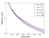
(a)

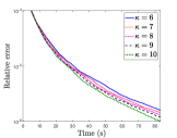
(b)

Figure 1. Comparison of Algorithm 1 with $\tau=\sigma_{1}=\sigma_{2}=\kappa/(10\sqrt{1+\|\nabla\|^{2}}))$, for image reconstruction from observation $b_{13}$.

Next, we compare Algorithm 1 when $\tau\sigma_{1}\|\nabla\|^{2}+\tau\sigma_{2}=1$, with alternative algorithms in [24, Theorem 3.3], [24, Theorem 3.1] or [55, Corollary 4.2], [12, Theorem 3.1], and [44], which are called “Condat”, “Condat-Vũ”, “MS”, and “AFBS”, respectively. In order to provide a fair comparison in our example, we approximate the best step-sizes by considering a mesh on the feasible set defined by the conditions allowing convergence for each algorithm. In the case when $\varepsilon=10^{-6}$, the best performance of Condat-Vũ is obtained by setting $\tau=1.2$ and $\sigma=0.99\cdot(2-\tau)/(2\tau\|\nabla\|^{2})$ which is next to the boundary of condition $\sigma\tau\|\nabla\|^{2}<(1-\tau/2)$. For MS, the performance is better when the only step-size $\tau$ is next to the boundary of the condition $\tau<1/\sqrt{1+\|\nabla\|^{2}}$, which leads us to set $\tau=0.99/\sqrt{1+\|\nabla\|^{2}}$. For AFBS, we found as best parameters $\tau=0.13$ and $\lambda_{n}\equiv 1.7/(65n+10)^{0.505}$ (see [44]). In the case of Condat, we consider 34 cases of parameters $\tau$ and $\sigma$ satisfying $\sigma\tau(1+\|\nabla\|^{2})=1$, by setting $\tau_{k}=\delta^{k}/(800\sqrt{1+\|\nabla\|^{2}})$ and $\sigma_{k}=800/(\delta^{k}\sqrt{1+\|\nabla\|^{2}})$, where $\delta=800^{1/8}$ and $k\in\{1,\ldots,34\}$. For Algorithm 1 we consider the same parameters $(\tau_{k})_{1\leq k\leq 34}$ than those in Condat, and we set $\sigma_{1,k}^{\ell}=(1-\ell)/(\tau_{k}\|\nabla\|^{2})$ and $\sigma_{2,k}^{\ell}=\ell/\tau_{k}$, for $\ell\in 10^{-1}\cdot\{5,0.1,0.05,0.01,0.005,0.003\}$, in view of (5.4). In Table 2 we provide the averages of CPU time, number of iterations, and the percentage of error between objective values $F^{TV}(\overline{x})$ and $F^{TV}(x_{n})$ obtained by previous algorithms with tolerance $\varepsilon=10^{-6}$ considering the observations $(b_{i})_{1\leq i\leq 20}$. We show the best 5 cases for Algorithm 1 ($k\in\{20,\ldots,24\}$) and the best case for Condat ($k=22$). We observe that Algorithm 1 and Condat reduce drastically the computational time and iterations obtained in Table 1, which shows the advantage of searching optimal parameters in the boundary of the condition of convergence. We also observe in Table 2 that Algorithm 1 ($k=22$ and $\ell=0.001$) is the most efficient method for this tolerance, followed closely by Condat ($k=22$). Both methods outperform drastically the competitors. In Figure 2 we show the relative error versus iterations and time for the observation $b_{13}$, confirming previous results.

Table 2. Averages of CPU time, number of iterations, and percentage of error in the objective value for Algorithm 1 with $\tau\sigma_{1}\|\nabla\|^{2}+\tau\sigma_{2}=1$, Condat, Condat-Vũ, AFBS, and MS with tolerance $10^{-6}$.

			$\varepsilon=10^{-6}$
Algorithm	$\tau$	$\sigma_{1}$	Av. Time(s)	Av. Iter.	Av. % error o.v.
Alg.1	0.77	0.16	21.12	4106	0.3531
	1.17	0.11	15.33	3223	0.3562
	1.77	0.07	13.97	2787	0.3649
	2.69	0.05	14.36	2891	0.3771
	4.09	0.03	16.23	3372	0.3907
Condat	1.77	-	14.89	2853	0.3673
Condat-Vũ	1.2	-	28.19	3539	0.3738
MS	0.33	-	62.48	6193	0.3506
AFBS	0.13	-	85.76	11104	0.6611

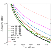
(a)

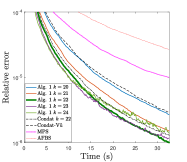
(b)

Figure 2. Comparison of Algorithm 1 with $\tau\sigma_{1}\|\nabla\|^{2}+\tau\sigma_{2}=1$, Condat, Condat-Vũ, AFBS, and MS (observation $b_{13}$).

In order to make a more precise comparison of Algorithm 1 and Condat, we consider a smaller tolerance $\varepsilon=10^{-8}$. The obtained results are shown in Table 3 and Figure 3. We observe that Algorithm 1 ($k=21$ and $\ell=0.001$) achieves the tolerance in approximately $11\%$ less CPU time than Condat in its best case ($k=21$). The efficiency in the case of the observation $b_{13}$ is illustrated in Figure 3.

Table 3. Averages of CPU time, number of iterations, and percentage of error in the objective value for Algorithm 1 with $\tau\sigma_{1}\|\nabla\|^{2}+\tau\sigma_{2}=1$ and Condat with tolerance $10^{-8}$.

			$\varepsilon=10^{-8}$
Algorithm	$\tau$	$\sigma_{1}$	Av. Time(s)	Av. Iter.	Av. % error o.v.
Alg. 1	0.77	0.16	93.36	19560	0.3514
	1.17	0.11	83.15	17561	0.3515
	1.77	0.07	100.06	20796	0.3515
	2.69	0.05	128.80	26801	0.3516
	4.09	0.03	160.92	33709	0.3517
Condat	1.17	-	93.77	18451	0.3515

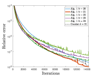
(a)

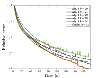
(b)

Figure 3. Comparison of Algorithm 1 with $\tau\sigma_{1}\|\nabla\|^{2}+\tau\sigma_{2}=1$ and Condat (observation $b_{13}$).

The reconstructed images, after 100 iterations, for the different algorithms are shown in Figure (4). The best reconstruction, in terms of objective value $F^{TV}$ and PSNR (Peak signal-to-noise ratio), are obtained by Condat and Algorithm 1.

(a)

(b)

(c)

(d)

(e)

(f)

(g)

Figure 4. Reconstructed image, after 100 iterations, from blurred and noisy image using AFBS, MS, Condat-Vũ, Condat and Alg. 1.

5.2. Split-ADMM in an academical example

In this section, we implement Algorithm 4.5, Corollary 4.10, and ADMM in (4.24) for solving an academical example in the context of Example 4.2. We compare their performances when solving the following optimization problem

$$\min_{x\in\mathbb{R}^{N}}F(x)=h(x-z)+\alpha\|Mx\|_{1},$$ (5.5)

where $h:\mathbb{R}^{N}\to\mathbb{R}$ is defined by

$$h\colon x=(\xi_{i})_{1\leq i\leq n}\mapsto\sum_{i=1}^{N}\phi(\xi_{i}),\quad\phi:\mathbb{R}\to\mathbb{R}\colon\xi\mapsto\begin{cases}|\xi|-\dfrac{\delta}{2},&\text{ if }|\xi|>\delta;\\ \dfrac{\xi^{2}}{2\delta},&\text{ if }|\xi|\leq\delta,\end{cases}$$ (5.6)

$\delta>0$, $z\in\mathbb{R}^{N}$, $\alpha>0$, and $M$ is a $N\times N$ symmetric positive definite real matrix. The first term in (5.5) is a data fidelity penalization using the Huber distance and the second term imposes sparsity in the solution. This type of problems appears naturally in image and signal denoising (see, e.g., [21, 42, 46, 50]).

Since $M$ is symmetric, there exist $N\times N$ real matrices $P$ and $D$, such that $P^{\top}=P^{-1}$, $D$ is diagonal, and $M=PDP^{\top}$. By setting $g=h(\cdot-z)$, $f=\alpha\|\cdot\|_{1}$, $K=PD^{1-\eta}P^{\top}$, and $T=PD^{\eta}P^{\top}$, for some $\eta\in\left[0,1\right]$, we deduce that $KT=M$ and (5.5) is a particular instance of ($P$). Next, we illustrate the efficiency of Algorithm 4.5 for different values of $\eta\in\left[0,1\right]$. Observe that, in the case when $\eta=0$ we have $T=\textnormal{Id}$ and Algorithm 4.5 reduces to the algorithm in Corollary 4.10. On the other hand, in the case when $\eta=1$ we have $K=\textnormal{Id}$ and Algorithm 4.5 reduces to ADMM in (4.24). We have $\text{\rm prox}_{f}\colon(\xi_{i})_{1\leq i\leq n}\mapsto\text{\rm prox}_{|\cdot|}(\xi_{i})$, where $\text{\rm prox}_{|\cdot|}$ is the scalar soft-thresholder operator [3, Example 24.34(iii)]. Note that, since $\ker T=\{0\}$, for every $\eta\in\left[0,1\right]$, the optimization problem in the second step of (4.6) admits a unique solution, in view of Remark 4.9(3). Therefore, when $\varUpsilon=\tau\textnormal{Id}$ and $\Sigma=\sigma\textnormal{Id}$, Algorithm 4.5 in this example reads as follows.

Algorithm 2

1:  Fix $\tau>0$, $p_{0},q_{0},x_{0}\in\mathbb{R}^{N}$, $\varepsilon>0$, and $r_{0}>\varepsilon$.

2:  while  $r_{n}>\varepsilon$ do

3:      $y_{n}=\!x_{n}+\tau(KTp_{n}-q_{n})$

4:     $p_{n+1}=\!\textnormal{zer}\big{(}\sigma\nabla h(\cdot-z)+T^{*}\big{(}T\cdot-(Tp_{n}-\sigma K^{*}y_{n})\big{)}\big{)}$

5:     $q_{n+1}=\text{\rm prox}_{f/\tau}(x_{n}/\tau+KTp_{n+1})$

6:      $x_{n+1}=x_{n}+\tau(KTp_{n+1}-q_{n+1})$

7:      $u_{n+1}=\sigma K^{*}(x_{n+1}-x_{n})-Tp_{n+1}$

8:      $r_{n+1}=\mathcal{R}(x_{n+1},u_{n+1},x_{n},u_{n})$

9:  end while

10:  return  $(p_{n+1},q_{n+1},x_{n+1})$

Note that the step 4 in Algorithm 2 involves the resolution of a non-linear equation when $\eta>0$. On the other hand, in the case when $\eta=0$, we have $T=\textnormal{Id}$ and, as noticed in Remark 4.11(3), the step 4 can be computed explicitly by using $\text{\rm prox}_{g}=z+\text{\rm prox}_{h}(\cdot-z)$ [3, Proposition 23.17(iii)] and the fact that $\delta h$ is the real Huber function (see [3, Example 8.44 & Example 24.9]). We consider as stopping criterion the primal-dual relative error defined in (5.3).

We compare the performance of Algorithm 2 when $\eta\in\{0,0.8,0.9,1\}$ with the standard solver fmincon of MATLAB for $N\in\{100,250,500\}$ and different values of the minimum and maximum eigenvalues $\lambda_{\max}\geq\lambda_{\min}>0$ of the matrix $M$. Since the expected value of $\lambda_{\max}$ (resp. $\lambda_{\min}$) of random matrices generated by a normal distribution increases (resp. decreases) as $N$ increases (see [32, Table 1.2]), we consider three classes of matrices with condition number $\kappa=\lambda_{\max}/\lambda_{\min}=50$ for each dimension $N\in\{100,250,500\}$:

• Class A: Class of matrices $M$ with small eigenvalues ($\lambda_{\max}=N/1000$).

• Class B: Class of matrices $M$ with average eigenvalues ($\lambda_{\max}=4N$).

• Class C: Class of matrices $M$ with large eigenvalues ($\lambda_{\max}=100N$).

For each class, we generate 30 random matrices using the randn function of MATLAB and the eigenvalues of each randomly generated matrix $M$ is forced to satisfy the conditions of each class after a singular value decomposition $M=PDP^{\top}$. We next generate $T$ and $K$ as described before. Step 4 in Algorithm 2 is computed via fsolve function of MATLAB (for $\eta>0$). We define the percentage of improvement of an algorithm with respect to fmincon via $I_{\bar{n}}=(\overline{F}-F(p_{\bar{n}}))\cdot 100/\overline{F},$ where $\overline{F}$ stands for the value of the function obtained by fmincon with tolerance $10^{-14}$ and $F(p_{\bar{n}})$ is the value of the function obtained by Algorithm 2 when it stops in iteration $\bar{n}$. Finally, we set the tolerance $\varepsilon=10^{-6}$ and $\tau=1$ in Algorithm 2.

Table 4 provides the averages of CPU time, iterations, and percentage of improvement with respect to fmincon of Algorithm 2 in the cases $\eta\in\{0,0.8,0.9,1\}$ for the 30 random matrices in each class and $N\in\{100,250,500\}$. We split our analysis of the results in the three classes of random matrices.

The best performance in the class A (small eigenvalues) is obtained by the case when $\eta=0$ (Corollary 4.10) in each dimension. The function value is very close to the one obtained by fmincon (difference of $10^{-5}$%). For this class, the cases when $\eta\in\{0.8,0.9\}$ are less accurate and ADMM ($\eta=1$) is even more precise but much slower than the case when $\eta=0$ for this class. This is explained by a very low cost per iteration and a comparable average number of iterations of the case when $\eta=0$.

On the other hand, for matrices belonging to the class B (average eigenvalues), the most efficient method is SADMM with $\eta=0.9$. The method needs very few number of iterations on average and it is more accurate than fmincon, since $I_{\bar{n}}$ is positive. This feature is also verified in $\eta\in\{0.8,1\}$ but the number of iterations and computational time is larger. We observe that the case when $\eta=0$ shows a very large number of iterations for achieving convergence and looses precision as the dimension increases. We conclude that SADMM outperforms drastically ADMM and the algorithm of Corollary 4.10, for suitable factorizations of matrices $M$ with average eigenvalues.

Finally, ADMM ($\eta=1$) is the best algorithm for the class C. It needs a very few number of iterations on average for achieving convergence, which nicely scales with the dimension. The computational time is around $1/3$ of the closest competitor and the precision is as good as fmincon. SADMM algorithms when $\eta\in\{0.8,0.9\}$ are similarly accurate but much slower. The case when $\eta=0$ is very far from the solution and extremely slow for this class in all dimensions.

Table 4. Performance of Algorithm 2 for $N\in\{100,250,500\}$, $\eta\in\{0,0.8,0.9,1\}$ and classes A, B, and C.

$N$	Class	$\eta$	$0$	$0.8$	$0.9$	$1$
100	A	Av. time	0.019	4.86	4.92	4.37
		Av. iter	688	704	717	656
		Av. $I_{\bar{n}}$ (%)	-$1.8\cdot 10^{-5}$	-0.47	-0.07	-$1.5\cdot 10^{-6}$
	B	Av. time	17.52	1.15	0.50	5.41
		Av. iter	798258	118	49	519
		Av. $I_{\bar{n}}$ (%)	0.63	0.36	0.33	0.64
	C	Av. time	31.44	3.77	1.07	0.34
		Av. iter	1410638	395	107	30
		Av. $I_{\bar{n}}$ (%)	-1607	-$8.4\cdot 10^{-8}$	-$8.1\cdot 10^{-8}$	-$5.1\cdot 10^{-8}$
250	A	Av. time	0.036	8.94	9.25	8.88
		Av. iter	380	359	387	393
		Av. $I_{\bar{n}}$ (%)	-$1.6\cdot 10^{-5}$	-1.03	-0.18	-$8\cdot 10^{-6}$
	B	Av. time	136.82	5.54	2.61	32.15
		Av. iter	1547593	143	64	886
		Av. $I_{\bar{n}}$ (%)	-0.15	0.18	0.19	0.25
	C	Av. time	85.28	27.14	5.83	1.76
		Av. iter	971230	761	120	39
		Av. $I_{\bar{n}}$ (%)	-18287	-$1.3\cdot 10^{-7}$	-$9.5\cdot 10^{-8}$	-$3.3\cdot 10^{-8}$
500	A	Av. time	0.067	13.41	13.58	13.52
		Av. iter	123	128	129	132
		Av. $I_{\bar{n}}$ (%)	$7.2\cdot 10^{-5}$	-1.47	-0.30	$8.2\cdot 10^{-5}$
	B	Av. time	581.25	39.99	23.95	113.24
		Av. iter	1249041	248	162	740
		Av. $I_{\bar{n}}$ (%)	-2.32	0.13	0.13	0.15
	C	Av. time	205.34	193.95	32.09	12.31
		Av. iter	419896	1200	182	46
		Av. $I_{\bar{n}}$(%)	-261808	-$1.8\cdot 10^{-7}$	-$1.5\cdot 10^{-7}$	-$9.4\cdot 10^{-8}$

References

- [1] T. Aspelmeier, C. Charitha, and D. R. Luke, Local linear convergence of the ADMM/Douglas-Rachford algorithms without strong convexity and application to statistical imaging, SIAM J. Imaging Sci., 9 (2016), pp. 842–868.
- [2] J.-P. Aubin and H. Frankowska, Set-valued analysis, vol. 2 of Systems & Control: Foundations & Applications, Birkhäuser Boston, Inc., Boston, MA, 1990.
- [3] H. H. Bauschke and P. L. Combettes, Convex Analysis and Monotone Operator Theory in Hilbert Spaces, CMS Books in Mathematics/Ouvrages de Mathématiques de la SMC, Springer, Cham, second ed., 2017.
- [4] R. I. Boţ and E. R. Csetnek, ADMM for monotone operators: convergence analysis and rates, Adv. Comput. Math., 45 (2019), pp. 327–359.
- [5] R. I. Boţ, E. R. Csetnek, and A. Heinrich, A primal-dual splitting algorithm for finding zeros of sums of maximal monotone operators, SIAM J. Optim., 23 (2013), pp. 2011–2036.
- [6] R. I. Boţ and C. Hendrich, A Douglas-Rachford type primal-dual method for solving inclusions with mixtures of composite and parallel-sum type monotone operators, SIAM J. Optim., 23 (2013), pp. 2541–2565.
- [7] S. Boyd, N. Parikh, E. Chu, B. Peleato, and J. Eckstein, Distributed optimization and statistical learning via the alternating direction method of multipliers, Foundations and Trends in Machine Learning, 3 (2011), pp. 1–122.
- [8] K. Bredies and H. Sun, Preconditioned Douglas-Rachford splitting methods for convex-concave saddle-point problems, SIAM J. Numer. Anal., 53 (2015), pp. 421–444.
- [9] K. Bredies and H. Sun, A proximal point analysis of the preconditioned alternating direction method of multipliers, J. Optim. Theory Appl., 173 (2017), pp. 878–907.
- [10] K. Bredies and H. P. Sun, Preconditioned Douglas-Rachford algorithms for TV- and TGV-regularized variational imaging problems, J. Math. Imaging Vision, 52 (2015), pp. 317–344.
- [11] L. Briceño, R. Cominetti, C. E. Cortés, and F. Martínez, An integrated behavioral model of land use and transport system: a hyper-network equilibrium approach, Netw. Spat. Econ., 8 (2008), pp. 201–224.
- [12] L. M. Briceño-Arias and P. L. Combettes, A monotone + skew splitting model for composite monotone inclusions in duality, SIAM J. Optim., 21 (2011), pp. 1230–1250.
- [13] L. M. Briceño Arias and P. L. Combettes, Monotone operator methods for Nash equilibria in non-potential games, in Computational and analytical mathematics, vol. 50 of Springer Proc. Math. Stat., Springer, New York, 2013, pp. 143–159.
- [14] L. M. Briceño-Arias and D. Davis, Forward-backward-half forward algorithm for solving monotone inclusions, SIAM J. Optim., 28 (2018), pp. 2839–2871.
- [15] L. M. Briceño-Arias and F. Roldán, Primal-dual splittings as fixed point iterations in the range of linear operators, 2019, https://arxiv.org/abs/1910.02329.
- [16] A. Chambolle, An algorithm for total variation minimization and applications, J. Math. Imaging Vision, 20 (2004), pp. 89–97, https://doi.org/10.1023/B:JMIV.0000011320.81911.38.
- [17] A. Chambolle, V. Caselles, D. Cremers, M. Novaga, and T. Pock, An introduction to total variation for image analysis, in Theoretical Foundations and Numerical Methods for Sparse Recovery, vol. 9 of Radon Ser. Comput. Appl. Math., Walter de Gruyter, Berlin, 2010, pp. 263–340.
- [18] A. Chambolle and P.-L. Lions, Image recovery via total variation minimization and related problems, Numer. Math., 76 (1997), pp. 167–188.
- [19] A. Chambolle and T. Pock, A first-order primal-dual algorithm for convex problems with applications to imaging, J. Math. Imaging Vision, 40 (2011), pp. 120–145.
- [20] G. Chen and M. Teboulle, A proximal-based decomposition method for convex minimization problems, Math. Programming, 64 (1994), pp. 81–101.
- [21] J. Colas, N. Pustelnik, C. Oliver, P. Abry, J.-C. Géminard, and V. Vidal, Nonlinear denoising for characterization of solid friction under low confinement pressure, Physical Review E , 42 (2019), p. 91.
- [22] P. L. Combettes, Quasi-Fejérian analysis of some optimization algorithms, in Inherently Parallel Algorithms in Feasibility and Optimization and their Applications (Haifa, 2000), vol. 8 of Stud. Comput. Math., North-Holland, Amsterdam, 2001, pp. 115–152.
- [23] P. L. Combettes and B. C. Vũ, Variable metric forward-backward splitting with applications to monotone inclusions in duality, Optimization, 63 (2014), pp. 1289–1318.
- [24] L. Condat, A primal-dual splitting method for convex optimization involving Lipschitzian, proximable and linear composite terms, J. Optim. Theory Appl., 158 (2013), pp. 460–479.
- [25] D. Dũng and B. C. Vũ, A splitting algorithm for system of composite monotone inclusions, Vietnam J. Math., 43 (2015), pp. 323–341.
- [26] I. Daubechies, M. Defrise, and C. De Mol, An iterative thresholding algorithm for linear inverse problems with a sparsity constraint, Comm. Pure Appl. Math., 57 (2004), pp. 1413–1457.
- [27] J. Douglas, Jr. and H. H. Rachford, Jr., On the numerical solution of heat conduction problems in two and three space variables, Trans. Amer. Math. Soc., 82 (1956), pp. 421–439.
- [28] J. Eckstein, Splitting Methods for Monotone Operators with Applications to Parallel Optimization, PhD thesis, Massachusetts Institute of Technology, 1989.
- [29] J. Eckstein and D. P. Bertsekas, On the Douglas-Rachford splitting method and the proximal point algorithm for maximal monotone operators, Math. Programming, 55 (1992), pp. 293–318.
- [30] J. Eckstein and B. F. Svaiter, A family of projective splitting methods for the sum of two maximal monotone operators, Math. Program., 111 (2008), pp. 173–199.
- [31] J. Eckstein and W. Yao, Understanding the convergence of the alternating direction method of multipliers: theoretical and computational perspectives, Pac. J. Optim., 11 (2015), pp. 619–644.
- [32] A. Edelman, Eigenvalues and condition numbers of random matrices, SIAM J. Matrix Anal. Appl., 9 (1988), pp. 543–560.
- [33] M. Fukushima, The primal Douglas-Rachford splitting algorithm for a class of monotone mappings with application to the traffic equilibrium problem, Math. Programming, 72 (1996), pp. 1–15.
- [34] D. Gabay, Chapter IX applications of the method of multipliers to variational inequalities, in Augmented Lagrangian Methods: Applications to the Numerical Solution of Boundary-Value Problems, M. Fortin and R. Glowinski, eds., vol. 15 of Studies in Mathematics and Its Applications, Elsevier, 1983, pp. 299 – 331.
- [35] D. Gabay and B. Mercier, A dual algorithm for the solution of nonlinear variational problems via finite element approximation, Computers & Mathematics with Applications, 2 (1976), pp. 17–40.
- [36] E. M. Gafni and D. P. Bertsekas, Two-metric projection methods for constrained optimization, SIAM J. Control Optim., 22 (1984), pp. 936–964.
- [37] R. Glowinski and A. Marrocco, Sur l’approximation, par éléments finis d’ordre un, et la résolution, par pénalisation-dualité, d’une classe de problèmes de Dirichlet non linéaires, Rev. Française Automat. Informat. Recherche Opérationnelle Sér. Rouge Anal. Numér., 9 (1975), pp. 41–76.
- [38] A. A. Goldstein, Convex programming in Hilbert space, Bull. Amer. Math. Soc., 70 (1964), pp. 709–710.
- [39] P. C. Hansen, J. G. Nagy, and D. P. O’Leary, Deblurring images: Matrices, spectra, and filtering, vol. 3 of Fundamentals of Algorithms, Society for Industrial and Applied Mathematics (SIAM), Philadelphia, PA, 2006.
- [40] B. He and X. Yuan, Convergence analysis of primal-dual algorithms for a saddle-point problem: from contraction perspective, SIAM J. Imaging Sci., 5 (2012), pp. 119–149.
- [41] P.-L. Lions and B. Mercier, Splitting algorithms for the sum of two nonlinear operators, SIAM J. Numer. Anal., 16 (1979), pp. 964–979.
- [42] X. Liu, D. Zhai, D. Zhao, G. Zhai, and W. Gao, Progressive image denoising through hybrid graph Laplacian regularization: a unified framework, IEEE Trans. Image Process., 23 (2014), pp. 1491–1503.
- [43] R. V. Mises and H. Pollaczek-Geiringer, Praktische verfahren der gleichungsauflösung, Zeitschrift für Angewandte Mathematik und Mechanik, 9 (1929), pp. 152–164.
- [44] C. Molinari, J. Peypouquet, and F. Roldan, Alternating forward-backward splitting for linearly constrained optimization problems, Optim. Lett., 14 (2020), pp. 1071–1088.
- [45] W. M. Moursi and Y. Zinchenko, A note on the equivalence of operator splitting methods, in Splitting Algorithms, Modern Operator Theory, and Applications, Springer, Cham, 2019, pp. 331–349.
- [46] J. Pang and G. Cheung, Graph Laplacian regularization for image denoising: analysis in the continuous domain, IEEE Trans. Image Process., 26 (2017), pp. 1770–1785.
- [47] T. Pock and A. Chambolle, Diagonal preconditioning for first order primal-dual algorithms in convex optimization, in 2011 International Conference on Computer Vision, 2011, pp. 1762–1769.
- [48] F. Riesz and B. Sz.-Nagy, Functional analysis, Frederick Ungar Publishing Co., New York, 1955.
- [49] L. I. Rudin, S. Osher, and E. Fatemi, Nonlinear total variation based noise removal algorithms, Phys. D, 60 (1992), pp. 259–268.
- [50] L. Sha, D. Schonfeld, and J. Wang, Graph Laplacian regularization with sparse coding for image restoration and representation, IEEE Transactions on Circuits and Systems for Video Technology, 30 (2020), pp. 2000–2014.
- [51] R. Shefi and M. Teboulle, Rate of convergence analysis of decomposition methods based on the proximal method of multipliers for convex minimization, SIAM J. Optim., 24 (2014), pp. 269–297.
- [52] R. E. Showalter, Monotone Operators in Banach Space and Nonlinear Partial Differential Equations, vol. 49 of Mathematical Surveys and Monographs, American Mathematical Society, Providence, RI, 1997.
- [53] B. F. Svaiter, On weak convergence of the Douglas-Rachford method, SIAM J. Control Optim., 49 (2011), pp. 280–287.
- [54] A. Themelis and P. Patrinos, Douglas-Rachford splitting and ADMM for nonconvex optimization: tight convergence results, SIAM J. Optim., 30 (2020), pp. 149–181.
- [55] B. C. Vũ, A splitting algorithm for dual monotone inclusions involving cocoercive operators, Adv. Comput. Math., 38 (2013), pp. 667–681.
- [56] M. Yan and W. Yin, Self equivalence of the alternating direction method of multipliers, in Splitting Methods in Communication, Imaging, Science, and Engineering, Sci. Comput., Springer, Cham, 2016, pp. 165–194.
- [57] Y. Yang, Y. Tang, M. Wen, and T. Zeng, Preconditioned Douglas-Rachford type primal-dual method for solving composite monotone inclusion problems with applications, Inverse Problems & Imaging, 15 (2021), pp. 787–825.
- [58] X. Zhang, M. Burger, and S. Osher, A unified primal-dual algorithm framework based on Bregman iteration, J. Sci. Comput., 46 (2011), pp. 20–46.