The AL-Gaussian Distribution as the Descriptive Model for the Internal Proactive Inhibition in the Standard Stop Signal Task

Abstract

Measurements of response inhibition components of reactive inhibition and proactive inhibition within the stop-signal paradigm have been of particular interest to researchers since the 1980s. While frequentist nonparametric and Bayesian parametric methods have been proposed to precisely estimate the entire distribution of reactive inhibition, quantified by stop signal reaction times(SSRT), there is no method yet in the stop-signal task literature to precisely estimate the entire distribution of proactive inhibition. We introduce an Asymmetric Laplace Gaussian (ALG) model to describe the distribution of proactive inhibition. The proposed method is based on two assumptions of independent trial type(go/stop) reaction times and Ex-Gaussian (ExG) models. Results indicated that the four parametric, ALG model uniquely describes the proactive inhibition distribution and its key shape features; and, its hazard function is monotonically increasing, as are its three parametric ExG components. In conclusion, both response inhibition components can be uniquely modeled via variations of the four parametric ALG model described with their associated similar distributional features.

1 Introduction

Response inhibition refers to one’s ability to stop responses or impulses that just became inappropriate or unwanted within continually changing environments,[1]. This process’s importance lies in one’s being in continually changing conditions, which require new, updated courses of action,[2]. Some instances of response inhibition in daily life include braking while driving a vehicle into an intersection in reaction to a sudden traffic change, changing direction during a tennis game, and resisting an extra piece of pizza at a birthday party. Two paradigms have been proposed to study the lab setting’s response inhibition, [3]: the stop-signal task and the Go/No-go task. In the standard stop-signal task, as used in this study, the task consists of a two-choice, response time task called the “go task” and the “stop task.” The go task is the primary task in which the participants are asked to correctly press a right or left button, in response to stimulus presentation, an “X” or “O” on the computer screen. The stop task is the occasional, secondary task in which (with a probability of stop signal $p_{ss}$ ) the participants are presented with a stop signal alarm after a temporal delay; Participants are instructed to withhold their responses the ongoing go task. Successful response inhibition occurs when participants successfully withhold their response to the “X” or “O” on the screen in the stop task (Figure 1).

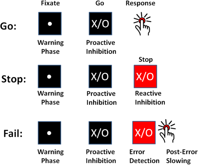
Figure 1: The standard stop signal task with two inhibition components: proactive inhibition, reactive inhibition [4]

Response inhibition has two distinctive temporal-dynamic components: reactive inhibition and proactive inhibition. Both components have been utilized within the standard stop-signal task, or its varieties, to discriminate different clinical groups, [5, 6]. We refer to reactive inhibition as the outright inhibition triggered by an external cause, while proactive inhibition is restraint of actions in preparation for stopping by external conditions, [7]. Each of these inhibition components have been quantified in distinctive methods as constant point estimate or distribution in the stop-signal task (SST) literature[1, 8, 9, 10, 11, 12, 13, 14, 15, 16, 17, 18, 19, 20, 21, 22, 23].

Reactive inhibition has been quantified as Stop Signal Reaction Times (SSRT) in the SST literature from both point estimation and distributional perspectives. Primary point estimations of the reactive inhibition up to now include the Crude SSRT, the Logan 1994 SSRT, [1], the Weighted SSRT, the Mixture SSRT, [8], and the time series-based SSRT,[9]. On the other hand, primary distributional estimations of the reactive inhibition include the Colonius’s nonparametric method,[10], the Bayesian Parametric Approach (BPA), [11, 12] — with two subtype methods: the Individual BPA (IBPA) and the Hierarchical BPA(HBPA) — and the mixture method, [13]. In the mixture method, the entire SST data is partitioned to type A SST data, trials following a go trial, and type B SST data, trials following a stop trial; The trial type weights are defined as $W_{A}^{c}=$proportion of type A stops within all stops, $W_{B}^{c}=1-W_{A}^{c}.$ Now, for $W_{A}\sim Bernoulli(W_{A}^{c}),W_{B}\sim Bernoulli(W_{B}^{c}),$ and fitted cluster type $SSRT_{A},SSRT_{B}$ distributions by the former two methods, the mixture index for the reactive inhibition is defined as:

$$SSRT_{Mixture}=^{d}W_{A}\times SSRT_{A}+W_{B}\times SSRT_{B}.$$ (1)

Note that for the case of parametric mixture SSRT, the cluster type components $SSRT_{A},$ and $SSRT_{B}$ may take a variety of proposed reaction time (RT) models, such as Ex-Gaussian (ExG), Ex-Wald, Wald, Gamma, Weibull, and lognormal, [14, 15, 16]. However, given the ExG model’s practical advantages to others, it is widely considered the parametric model for the reactive inhibition,[11, 12].

Proactive inhibition has been quantified in the SST literature merely as point estimation from different perspectives. The first such estimation is defined through a dynamic Bayesian model,[17]. Here, using the mixture assumption for the predictive distribution for the probability of the kth trial being a stop task $``p(Stop),”$ the reactive inhibition is defined as the following positive Pearson correlation called the ”Sequential Effect(SE)”:

$$SE = Corr(p(Stop),GORT).$$ (2)

The second estimation is based on the variation of differences of reaction times in a go trial (GORTs) in the associated arms of the modified standard stop signal task paradigm,[18, 19, 20, 21, 22, 23]. Generally, for two given probabilities of stop signals in two arms of the modified SST where $0\ll p_{ss}^{(1)}<p_{ss}^{(2)}\ll 1,$ the arm type proactive inhibition $\Delta_{AT}GORT$ is defined by as:

$$\Delta_{AT}GORT = mean(GORT_{(p_{ss}^{(2)})})-mean(GORT_{(p_{ss}^{(1)})}).$$ (3)

The last type of the point estimation of proactive inhibition is based on the differences of GORTs in the trial type clusters of the standard SST paradigm [8, 9](Figure.2.). Here, for the fixed stop signal probability (e.g.$p_{ss}=0.25$) and the type A GORTA and type B GORTB, the trial type proactive inhibition $\Delta_{TT}GORT$ is defined as:

$$\Delta_{TT}GORT = mean(GORT_{B})-mean(GORT_{A}).$$ (4)

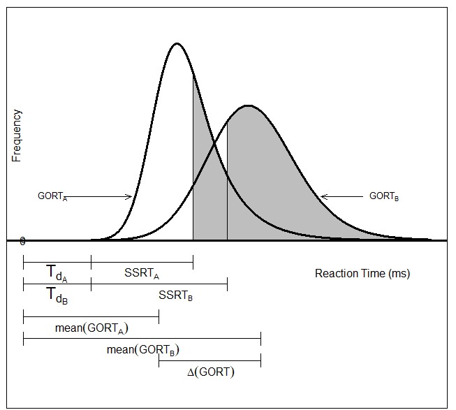
Figure 2: Trial type point estimation of proactive inhibition in the standard stop signal task

However, little information is available in the SST literature on the entire distribution of proactive inhibition and its key features. This subject is significant as measures of central tendencies, such as mean or median, are insufficient — and even unnecessary — to compare mostly skewed response inhibition distributions,[24]. Besides, masking prominent features of the proactive inhibitions by using central tendency measures may result in incorrect conclusions about their make-up. As an example, two different clinical groups may have the same mean of proactive inhibition, but the shape of their distributions may differ: one may be more positively skewed, or more leptokurtic, or possess a higher domain of variance. The methods mentioned earlier of the estimation of proactive inhibition do not allow for precise estimation and description of the appropriate models for the entire set of proactive inhibition distributions.

This study proposes a four parametric, Asymmetric Laplace Gaussian (ALG) model for the entire proactive inhibition, given the assumption of independent trial type (go/stop) GORTs within the standard stop-signal task. The study outline is as follows. First, as in [8, 9] the overall SST data for each participant is partitioned to type A SST data and type B SST data. Second, using the Individual Bayesian Parametric Approach (IBPA) method [11, 12], the fitted ExG GORT mean posterior parameters are calculated for the cluster type SST data. Then, the distribution of proactive response inhibition is introduced as the difference of two independent fitted GORT ExG models, and it is shown that it has a four-parametric ALG distribution. Third, the descriptive statistics, shape statistics, and vital distributional properties of the ALG model, such as component decomposition, shape and tail behavior, and monotonic hazard function, are discussed. Finally, an empirical example is presented to manifest the above-presented results. Table 1 presents the summary of estimations methods presented in the literature, including this study given the type of inhibition component.

Table 1: Summary of Estimation Methods of Inhibition Components

[b] Estimation Inhibition Component Reactive Proactive Constant Index SSRT $\Delta GORT$,$SE$ Examples $SSRT_{Crude},SSRT_{Mixture},SSRT_{Weighted}$ $\Delta_{AT}GORT,\Delta_{TT}GORT$ $SSRT_{Logan1994},SSRT_{SS.Logan1994}$ Distribution Index SSRT $\Delta GORT$ Examples ExG,LN,Wald ALG Ex-Wald, Gamma

2 Materials & Methods

2.1 Data

The study data have been previously described [25, 8, 9, 13]. Data were collected at the Ontario Science Center in Toronto, Canada, in 2009-2010. Included were 16,099 participants aged 6 to 17. The participants’ parents provided the required ethical consent for the SST experiment. Each participant completed the SST task, including four blocks of 24 trials with a total of 96 trials, including random 25% stop trials (24 stops) and 75% go trials(72 goes). The SST tracking algorithm was designed so that at the end of trials, each participant achieves a 50% probability of successful inhibition.

2.2 Participants

The study participants are the same as those described in [9, 13]. Included here is a unique subsample of 44 participants with a mean age of 12.1 years, with 96 SST trials for each, and an almost balanced number of trial type stop trials (10-14 type B stop trials vs. 14-10 type A stop trials, respectively). This almost balanced number of trial type stop trials yields 30-42 type B go trials vs. 42-30 type A stop trials, respectively.

2.3 The SST Clusters

The study Stop Signal Task clusters have been described before in [8, 9, 13]. Each participant’s SST data was partitioned to type A SST data, where a go trial preceded all trials, and type B SST data, all trials preceded by a stop trial. Hence, each participant has three types of SST data clusters: Type-A SST cluster (i.e., 56 trials), Type B SST cluster(i.e., 40 trials), and Type-S SST cluster (all 96 trials). Then, using IBPA, the parameters of the corresponding Ex-Gaussian (ExG) GORT’s parameters (i.e. $\theta_{A}=(\mu_{A},\sigma_{A},\tau_{A}),\theta_{B}=(\mu_{B},\sigma_{B},\tau_{B}),\theta_{S}=(\mu_{S},\sigma_{S},\tau_{S})$ were computed as described in the upcoming results section 3.2.

2.4 Preliminaries on Component Distributions

The first two definitions provide the critical features of the components of our upcoming calculations, namely Ex-Gaussian distribution (ExG), [26], and the Asymmetric Laplace distribution (AL), [27].

Definition 2.1.

A random variable has an Ex-Gaussian (ExG) distribution with parameters $(\mu,\sigma,\tau)$ whenever it is considered as the sum of an independent normal random variable with parameters $(\mu,\sigma^{2})$ and an exponential random variable with parameter $\tau$:

$$ExG(\mu,\sigma,\tau) =^{d} N(\mu,\sigma^{2})\oplus Exp(\tau).$$ (5)

The density, the moment generating function, the nth cumulant $(n\geq 1),$ the variance, the skewness and the kurtosis of the ExG distribution are given by:

$$PDF f_{ExG}(t|\mu,\sigma,\tau)=\frac{1}{\tau}exp(\frac{\mu-t}{\tau}+\frac{\sigma^{2}}{2\tau^{2}})*\Phi(\frac{\mu-t}{\sigma}-\frac{\sigma}{\tau}):\sigma,\tau>0,t\in\mathbb{R},$$

$$MGF m_{ExG}(t)=(1-t\tau)^{-1}exp(\mu.t+\frac{\sigma^{2}}{2}t^{2}):t<\tau^{-1},$$

$$n^{th}Cumulant \kappa_{n}^{ExG}=(n-1)!\tau^{n}+1_{n=1}(n)\mu+1_{n=2}(n)\sigma^{2}:1\leq n,$$

$$Mean E(ExG)=\mu+\tau,$$

$$Variance Var(ExG)=\sigma^{2}+\tau^{2},$$

$$Skewness \gamma_{ExG}=2(1+\sigma^{2}\tau^{-2})^{-3/2},$$

$$Kurtosis \kappa_{ExG}=3\frac{(1+2\sigma^{-2}\tau^{2}+3\sigma^{-4}\tau^{4})}{(1+\sigma^{-2}\tau^{2})^{2}}.$$ (6)

Definition 2.2.

A random variable has an Asymmetric Laplace (AL) distribution with parameters $(\alpha_{1},\alpha_{2})$ whenever it is considered as the difference of two independent exponential random variables with parameters $\alpha_{2}$, and $\alpha_{1}$, respectively:

$$AL(\alpha_{1},\alpha_{2}) =^{d} Exp(\alpha_{2})\ominus Exp(\alpha_{1}).$$ (7)

The density, the moment generating function, the nth cumulant $(n\geq 1),$ the variance, the skewness and the kurtosis of the AL distribution are given by:

$$PDF f_{AL}(t|\alpha_{1},\alpha_{2})=\frac{exp(\frac{t}{\alpha_{1}})1_{(-\infty,0)}(t)+exp(\frac{-t}{\alpha_{2}})1_{[0,\infty)}(t)}{\alpha_{1}+\alpha_{2}}\ t\in\mathbb{R},$$

$$MGF m_{AL}(t)=(1+(\alpha_{1}-\alpha_{2})t-\alpha_{1}\alpha_{2}.t^{2})^{-1}\ -\alpha_{1}^{-1}<t<\alpha_{2}^{-1},$$

$$n^{th}Cumulant \kappa_{n}^{AL}=(n-1)!((-\alpha_{1})^{n}+(\alpha_{2})^{n})\ 1\leq n,$$

$$Mean E(AL)=-(\alpha_{1}-\alpha_{2}),$$

$$Variance Var(AL)=\alpha_{1}^{2}+\alpha_{2}^{2},$$

$$Skewness \gamma_{AL}=-2(\alpha_{1}^{3}-\alpha_{2}^{3})\times(\alpha_{1}^{2}+\alpha_{2}^{2})^{-3/2},$$

$$Kurtosis \kappa_{AL}=3(3\alpha_{1}^{4}+2\alpha_{1}^{2}\alpha_{2}^{2}+3\alpha_{2}^{4})\times(\alpha_{1}^{2}+\alpha_{2}^{2})^{-2}.$$ (8)

The convolution of two independent, AL random variables and Gaussian random variables, called ALG or Normal-Laplace (NL) random variables, has been of special attention in the literature [28, 29].

Definition 2.3.

A random variable has Asymmetric Laplace-Gaussian (ALG) distribution with parameters $(\alpha_{1},\alpha_{2},\mu,\sigma)$ whenever it is considered as the sum of two independent, Asymmetric Laplace random variables with parameters $(\alpha_{1},\alpha_{2})$, and a Normal random variable with parameters $(\mu,\sigma^{2})$, respectively:

$$ALG(\alpha_{1},\alpha_{2},\mu,\sigma) =^{d} AL(\alpha_{1},\alpha_{2})\oplus N(\mu,\sigma^{2}).$$ (9)

Note that since $AL(0^{+},\alpha_{2})=^{d}Exp(\alpha_{2}),$ it follows that $ALG(0^{+},\alpha_{2},\mu,\sigma)=^{d}ExG(\mu,\sigma,\alpha_{2})$. Consequently, the ExG model can be considered a special degenerate ALG model. Next, the following key Theorems equip us to propose the ALG distribution as the model for the proactive inhibition and compute the key descriptive and shape statistics of the ALG distribution in terms of its Laplacian and Gaussian components,[30].

Theorem 2.4.

Let $X,Y$ be two independent, real-valued random variables with finite, moment generating function $m_{X},m_{Y},$ and cumulant functions $\kappa,\kappa,$ respectively. Then, for some $s_{0}>0:$

$$m_{X+Y}(t)=m_{X}(t)m_{Y}(t):\ \ (-s_{0}<t<s_{0}),$$ (10)

$$\kappa_{X+Y}(t)=\kappa_{X}(t)+\kappa(t):\ \ \ (-s_{0}<t<s_{0}).$$ (11)

Theorem 2.5.

Let $X,Y$ be two real-valued random variables with finite moment generating functions $m_{X},m_{Y},$ respectively. Assume for some $s_{0}>0:\ m_{X}(t)=m_{Y}(t)\ (-s_{0}<t<s_{0}).$ Then, $X,Y$ have the same distribution.

Finally, the last two theorems enable us to describe the behavior of the hazard function of the ALG model for the proactive inhibition, [31].

Theorem 2.6.

Let $X$ be a real-valued random variable with differentiable PDF $f_{X}$ and CDF $F_{X}$ such that $f_{X}(t)\rightarrow 0,F_{X}(t)\rightarrow 1\ as\ t\rightarrow\infty,$ and $-ln(f_{X}(t))$ is convex(concave). Then, the hazard function $h_{X}$ is increasing(decreasing).

Theorem 2.7.

Let $X,Y$ be two independent, real-valued random variables with (strictly) increasing hazard functions $h_{X},h_{Y},$ respectively. Then, the hazard function of their sum, $h_{X+Y}$ is (strictly) increasing as well.

2.5 Proactive Inhibition Index

Proactive inhibition was operationalized based on the standard stop signal task’s internal perspective,[9]. Here, for a given fixed stop signal probability (e.g., 0.25), type A GORT of $GORT_{A}$ (GORT for a trial after a go trial), and type B GORT of $GORT_{B}$ (GORT for a trial after a stop trial), the internal proactive inhibition is defined as:

$$\Delta GORT =^{d} GORT_{B}-GORT_{A}.$$ (12)

Note that there are two mathematical perspectives for the proactive inhibition: First, a model with two ExG components; Second, a model with Asymmetric Laplace (AL) and Gaussian components. Henceforward, it is understood within the given context which perspective is being discussed.

2.6 Statistical Analysis

The statistical ALG model to describe the proactive inhibition distribution was presented using moment generating functions, [29]. Next, the ALG model’s descriptive and shape statistics were computed in terms of parameters of the cluster type ExG components,[30]. Finally, its hazard function behavior was theoretically inferred using its components’ parameters [31].

The ExG components of the presented statistical model were estimated using the IBPA method,[11, 12]. As in [13], each participant had three IBPA associated ExG parametric estimations $\theta_{A}=(\mu_{A},\sigma_{A},\tau_{A}),\theta_{B}=(\mu_{B},\sigma_{B},\tau_{B}),$ and $\theta_{S}=(\mu_{S},\sigma_{S},\tau_{S}),$ associated to type-A cluster SST data, type-B cluster SST data, and the entire SST data, respectively. These parameters were estimated as the posterior means of the associated following IBPA procedure with three chains, 5,000 burn-ins within 20,000 simulations in Bayesian Ex-Gaussian Estimation of Stop-Signal RT distributions (BEESTS) 2.0 software,[12]:

Data	Individual Priors
$GORT\sim ExG(\mu_{go},\sigma_{go},\tau_{go})$
$SRRT\sim ExG(\mu_{go},\sigma_{go},\tau_{go},\mu_{stop},\sigma_{stop},\tau_{stop},SSD)I^{+}_{[1,1000]}$	$\mu_{go},\sigma_{go},\tau_{go}\sim U[10,2000]$
$SSRT\sim ExG(\mu_{go},\sigma_{go},\tau_{go},\mu_{stop},\sigma_{stop},\tau_{stop},SSD)I^{+}_{[1,1000]}$	$\mu_{go},\sigma_{go},\tau_{go}\sim U[10,2000]$

Two sets of comparisons were conducted using paired t-tests (DescTools, $R$ software version 4.0.0, [32]): First, a primary comparison between the cluster-type fitted parameter of the ExG distribution, the descriptive statistics, and the shape statistics; second, secondary comparisons between the ALG model descriptive and shape statistics and its associated cluster-type ExG components.

3 Results

The results are divided into two subsections. In subsection 3.1, we explore the mathematical analysis of the proposed model for the proactive inhibition in the standard stop-signal task. This model includes a four parametric ALG for the proactive inhibition and its prominent distributional properties. In subsection 3.2, we present an empirical example of the case and discuss its various distributional features.

3.1 Mathematical Analysis

3.1.1 The Proactive Inhibition Distribution and its Parameters

First of all, we propose a mathematical model for the proactive inhibition provided by the ALG:

Theorem 3.1.

(The Main Result). The four parametric $ALG(\tau_{A},\tau_{B},\mu_{B}-\mu_{A},(\sigma_{B}^{2}+\sigma_{A}^{2})^{1/2})$ presents a model for the Internal Proactive Inhibition Index $\Delta GORT$ with trial type-related parameters $(\mu_{A},\sigma_{A},\tau_{A},\mu_{B},\sigma_{B},\tau_{B})$ in the Standard Stop Signal Task.

As a corollary of Theorem 3.1, the probability density function $(f_{\Delta GORT})$ and the cumulative density function $(F_{\Delta GORT})$ of the ALG distribution for the Internal Proactive Inhibition Index are given by [28, 29],:

$$f_{\Delta GORT}(t) = \frac{1}{\tau_{A}+\tau_{B}}$$ (13)

$$\times[ e^{(\frac{\sqrt{\sigma_{B}^{2}+\sigma_{A}^{2}}}{2\tau_{B}}(\frac{\sqrt{\sigma_{B}^{2}+\sigma_{A}^{2}}}{\tau_{B}}-2\frac{t-(\mu_{B}-\mu_{A})}{\sqrt{\sigma_{B}^{2}+\sigma_{A}^{2}}}))}\times(1-\Phi(\frac{\sqrt{\sigma_{B}^{2}+\sigma_{A}^{2}}}{\tau_{B}}-\frac{t-(\mu_{B}-\mu_{A})}{\sqrt{\sigma_{B}^{2}+\sigma_{A}^{2}}}))$$

$$+ e^{(\frac{\sqrt{\sigma_{B}^{2}+\sigma_{A}^{2}}}{2\tau_{A}}(\frac{\sqrt{\sigma_{B}^{2}+\sigma_{A}^{2}}}{\tau_{A}}+2\frac{t-(\mu_{B}-\mu_{A})}{\sqrt{\sigma_{B}^{2}+\sigma_{A}^{2}}}))}\times(1-\Phi(\frac{\sqrt{\sigma_{B}^{2}+\sigma_{A}^{2}}}{\tau_{A}}+\frac{t-(\mu_{B}-\mu_{A})}{\sqrt{\sigma_{B}^{2}+\sigma_{A}^{2}}}))]$$

$$\hskip 284.52756ptt\in\mathbb{R}$$

and

$$F_{\Delta GORT}(t) = \frac{1}{\tau_{A}^{-1}+\tau_{B}^{-1}}\times[(\tau_{A}^{-1}+\tau_{B}^{-1})\Phi(\frac{t-(\mu_{B}-\mu_{A})}{\sqrt{\sigma_{B}^{2}+\sigma_{A}^{2}}})$$ (14)

$$- \tau_{A}^{-1}e^{(\frac{\sqrt{\sigma_{B}^{2}+\sigma_{A}^{2}}}{2\tau_{B}}(\frac{\sqrt{\sigma_{B}^{2}+\sigma_{A}^{2}}}{\tau_{B}}-2\frac{t-(\mu_{B}-\mu_{A})}{\sqrt{\sigma_{B}^{2}+\sigma_{A}^{2}}}))}\times(1-\Phi(\frac{\sqrt{\sigma_{B}^{2}+\sigma_{A}^{2}}}{\tau_{B}}-\frac{t-(\mu_{B}-\mu_{A})}{\sqrt{\sigma_{B}^{2}+\sigma_{A}^{2}}}))$$

$$+ \tau_{B}^{-1}e^{(\frac{\sqrt{\sigma_{B}^{2}+\sigma_{A}^{2}}}{2\tau_{A}}(\frac{\sqrt{\sigma_{B}^{2}+\sigma_{A}^{2}}}{\tau_{A}}+2\frac{t-(\mu_{B}-\mu_{A})}{\sqrt{\sigma_{B}^{2}+\sigma_{A}^{2}}}))}\times(1-\Phi(\frac{\sqrt{\sigma_{B}^{2}+\sigma_{A}^{2}}}{\tau_{A}}+\frac{t-(\mu_{B}-\mu_{A})}{\sqrt{\sigma_{B}^{2}+\sigma_{A}^{2}}}))]$$

$$\hskip 284.52756ptt\in\mathbb{R},$$

respectively. Here $\Phi$ denotes the standard normal cumulative distribution function.
Next, given trial type parameters, we estimate the descriptive and shape statistics for the proposed ALG model of the proactive inhibition:

Theorem 3.2.

The descriptive statistics and the shape statistics of the Proactive Inhibition ALG distribution with trial type-related parameters $(\mu_{A},\sigma_{A},\tau_{A},\mu_{B},\sigma_{B},\tau_{B})$ in the standard stop signal task are given by:

$$n^{th}Cumulant \kappa_{n}^{ALG}=(n-1)!((-\tau_{A})^{n}+\tau_{B}^{n})$$

$$\hskip 28.45274pt+1_{(n=1)}(n)(\mu_{B}-\mu_{A})+1_{(n=2)}(n)(\sigma_{B}^{2}+\sigma_{A}^{2}):\ \ 1\leq n$$

$$Mean E(ALG)=\tau_{B}-\tau_{A}+\mu_{B}-\mu_{A},$$

$$Variance Var(ALG)=\tau_{A}^{2}+\tau_{B}^{2}+\sigma_{A}^{2}+\sigma_{B}^{2},$$

$$Skewness \gamma_{ALG}=\frac{2(\tau_{B}^{3}-\tau_{A}^{3})}{(\tau_{A}^{2}+\tau_{B}^{2}+\sigma_{A}^{2}+\sigma_{B}^{2})^{3/2}},$$

$$Kurtosis \kappa_{ALG}=\frac{6(\tau_{B}^{4}+\tau_{A}^{4})}{(\tau_{A}^{2}+\tau_{B}^{2}+\sigma_{A}^{2}+\sigma_{B}^{2})^{2}}.$$ (15)

3.1.2 The Proactive Inhibition’s Key ALG Distributional Properties

In this section, we present key distributional properties for the ALG model for proactive inhibition including: (i) component decompositions in terms of trial type GORT; (ii) shape and tail behavior; and, (iii) behavior of the hazard function.

Theorem 3.3.

(Component Decomposition). An ALG model for proactive inhibition emerges from uncountable pairs of trial type related GORT $(GORT_{A},GORT_{B})$ distributions.

We remind the reader that Theorem3.3 presents a process to simulate a plausible four parametric ALG distribution for the proactive inhibition.

Theorem 3.4.

(Shape and Tail Behavior). An ALG model for proactive inhibition has unimodal, generally asymmetric, infinite, differentiable density with extreme large values proportionate to the $Exp(1/\tau_{B})$ distribution.

We remind the reader that contrary to the ALG model’s mean for proactive inhibition, there are no closed-form formulas for the mode and the median, respectively. Similar to the ExG model for reactive inhibition with increasing hazard function, we have:

Theorem 3.5.

(Hazard Function’s Behavior). An ALG model for proactive inhibition has increasing hazard function.

3.2 The Empirical Example

3.2.1 The ALG Model for Proactive Inhibition

This section presents an example of the empirical data for the theoretical results inferred in the previous section on the ALG model for proactive inhibition and its descriptive, shape, and hazard function’s key features. These results are based on the cluster type IBPA estimation of mean posterior ExG parameters $\theta=(\mu,\sigma,\tau)$ presented in Table 5(Appendix B).

The ExG model for each of the two components of proactive inhibition has the following key features presented by Table 2. First, while type B $\mu,$, and $\sigma$ parameters are significantly larger than their type A counterparts, there is no difference for the $\tau$ parameter. In addition, the sample average proactive inhibition is 92.1 ms (95% CI = (69.4,114.9)). Second, both ExG components are positively skewed and leptokurtic. Finally, there is no significant difference between their trial-type skewness and their trial-type kurtosis, respectively. Figure3a presents the trial type ExG modeled components of the ALG model.

Table 2: Descriptive and paired t-test [mean ($95\%CI$)] results for parameters, descriptive and shape statistics of fitted Ex-Gaussian distribution to cluster type GORT and AL-Gaussian distribution to $\Delta GORT,(n=44).$

[b] ExG model ALG model Cluster Comparison Cluster Type A Type B Type B vs. Type A Type S $\alpha_{1}$ - - - 104.2 - - - (90.4,117.9) $\alpha_{2}$ - - - 142.4 - - - (125.9,158.8) Parameter $\mu$ 478.8 532.8 53.9*** 53.9 (448.0,509.7) (498.6,566.9) (30.9,76.9) (30.9,76.9) $\sigma$ 109.9 133.1 23.2 179.2 (90.5,129.3) (108.4,157.8) (-0.1,46.4) (151.4,206.9) $\tau$ 104.2 142.4 38.2*** - (90.4,117.9) (125.9,158.8) (19.6,56.8) - Mean 583.0 675.1 92.1*** 92.1 (553.0,612.9) (633.8,716.4) (69.4,114.9) (69.4,114.9) Statistics St.D 160.6 202.4 41.8*** 260.4 (143.5,177.8) (177.9,226.9) (25.9,57.6) (232.3,288.6) Skewness 0.787 0.918 0.131 0.186 (0.602,0.973) (0.751,1.085) (-0.113,0.375) (0.076,0.296) Kurtosis 4.966 5.300 0.334 1.153 (4.414,5.518) (4.790,5.808) (-0.397,1.064) (0.923,1.384)

• Notes: ^∗p-value$<0.05$;^∗∗p-value$<0.005$;^∗∗∗p-value$<0.0005$.

The ALG model for proactive inhibition has the following features, given cluster type parameter estimations. First, as a primary corollary of Theorem 3.2, the model is positively skewed whenever $\tau_{B}>\tau_{A}.$ The negatively skewed and symmetric cases hold whenever the strict greater inequality $>$ is replaced with $<$ and $=,$ respectively. According to appendix Table  5 data, all three cases exist (case 10: positive skew; case 16: symmetric; case 11: negative skew). Figure 3b presents all the mentioned three cases. Overall, the model is positively skewed given the results in Table 2. Second, as the second corollary of Theorem 3.2, the model is leptokurtic whenever $(2(\tau_{A}^{4}+\tau_{B}^{4}))^{1/2}-(\tau_{A}^{2}+\tau_{B}^{2})>\sigma_{A}^{2}+\sigma_{B}^{2}.$ The platykurtic and mesokurtic cases hold whenever the strict greater inequality $>$ is replaced with $<$ and $=,$ respectively. In particular, for the case, $\tau_{A}\approx\tau_{B},$ the model is always platykurtic. Overall, the model is platykurtic given results in Table  2. Third, while the ALG model’s standard deviation is larger than its two ExG’s components, its skewness and kurtosis are significantly smaller. Finally, the ALG model has a strictly increasing hazard function for various skewness cases, as mentioned in Theorem3.5 and presented in Figure 3c.

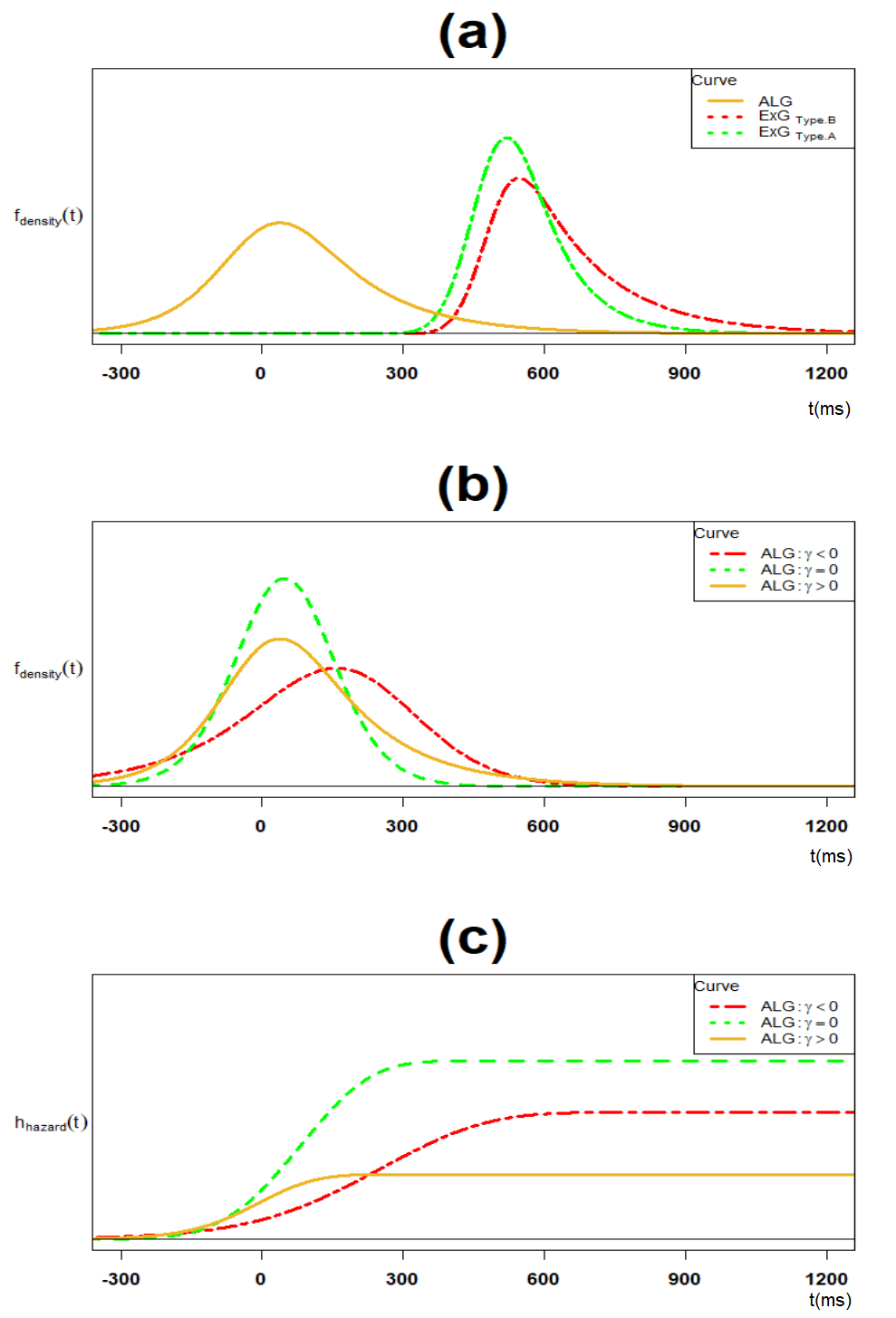
Figure 3: The ALG density and its trial type ExG component densities; (b) The ALG density for the positively skewed, symmetric and negatively skewed cases; (c) The ALG hazard function for the positively skewed, symmetric and negatively skewed cases.

3.2.2 Proactive Inhibition ALG Model versus Reactive Inhibition ExG Model

This section compares the ALG distribution of the proactive inhibition and the ExG distribution of the reactive inhibition in descriptive and shapes statistics. Table 3 presents the corresponding statistics for both models. As it is seen, the proactive ALG inhibition distribution has a significantly lower mean, lower skewness, lower kurtosis, and higher standard deviation than reactive inhibition ExG distribution. Also, while the proactive inhibition ALG distribution is platykurtic, the corresponding reactive ExG distribution is leptokurtic. However, the two distributions are both positively skewed. Overall, the two distributions are significantly distinctive.

Table 3: Comparison of proactive inhibition ALG model versus reactive inhibition ExG model in terms of descriptive and shape statistics $(n=44).$

[b] Inhibition Reactive Proactive Proactive vs. Reactive Index $SSRT$ $\Delta GORT$ $\Delta GORT\ vs.\ SSRT$ Model ExG ALG ALG vs. ExG Mean 196.8 92.1 -104.6*** (173.5,220.1) (69.4,114.9) (-140.6,-68.7) Statistics St.D 157.8 260.4 102.6*** (139.4,176.2) (232.3,288.6) (71.8,133.6) Skewness 0.578 0.186 -0.401*** (0.500,0.674) (0.076,0.296) (-0.540,-0.261) Kurtosis 4.231 1.153 -3.077*** (3.998,4.465) (0.923,1.384) (-3.381,-2.775)

• Notes: ^∗p-value$<0.05$;^∗∗p-value$<0.005$;^∗∗∗p-value$<0.0005$.

4 Discussion

4.1 Present Work

This paper presents a four parametric model for the entire proactive inhibition distribution, the ALG model. This model is based on the two independent ExG components fitted to the trial type GORTs. Considering ExG models as a degenerate ALG model, this work indicates that a four parametric ALG model can model both response inhibition components.

The proposed ALG model for proactive inhibition has several important aspects. First, the model is based on the independent assumption of GORTA and GORTB. Such speculation is warranted by the independent assignment of go trials and stop trials in the entire stop-signal task trials. Hence, via conditioning, their following associated type A go trial and type B go trials are independent, and so are their associated GORTs (i.e., GORTA and GORTB). Second, contrary to the point estimations of proactive inhibition in the form of mean [9], or correlation [17], it presents the entire distribution of the proactive inhibition. Third, the ALG model for proactive inhibition is entirely distinctive from the ExG model for reactive inhibition in terms of the mean, standard deviation, and kurtosis. This result provides more evidence on the distinction between proactive inhibition and reactive inhibition as a whole distribution. Fourth, similar to the ExG model for reactive inhibition, the ALG model for proactive inhibition is skewed to the right and has a monotonically increasing hazard function. Finally, the ALG model for proactive inhibition with its associated ExG modeled components is unique because other non-ExG RT models for its components (e.g., Gamma, Weibull, Lognormal, Wald, and Ex-Wald) do not yield to any known closed-form distribution for proactive inhibition. This limitation is easily verifiable by repeating the proof of Theorem 3.1 based on the uniqueness of moment generating functions for other non-ExG RT models for the trial type GORTs.

The proposed ALG model for the proactive inhibition is estimated (or simulated) in two different methods. First, one may use the Bayesian or frequentist-based methods to fit the ExG parametric models to its trial-type components and then estimate the four parametric ALG model using Theorem 3.1, as done in Section 3.2. Second, one may subtract the trial type GORTs and fit the ALG model directly to the differenced GORT data using Maximum Likelihood (ML) or Expectation-Maximization (EM) algorithms [33].

The proposed ALG model uniquely distinguishes the reactive inhibition and proactive inhibition distribution in terms of vital distributional features. Table 4 presents an overall comparison for proactive inhibition and reactive inhibition in terms of the ALG model(with considering ExG as its particular case):

Table 4: Comparison of proactive inhibition and reactive inhibition in terms of ALG model properties.

[b] Inhibition Index $\#$ Parameters $\#$ Estimations Mean StD Skewness($+$) Kurtosis Hazard Proactive $\Delta GORT$ 4 2 lower higher lower platykurtic increasing Reactive $SSRT$ 3 1 higher lower higher leptokurtic increasing

There are some limitations in the proposed ALG model for proactive inhibition. First, since GORTA data and GORTB data are unmatched, there is no way to calculate their correlation quantitatively. Hence, from a quantitative perspective, checking the validity of the assumption of independent GORTA and GORTB is difficult. Second, by its definition, proactive inhibition takes only non-negative values while the presented ALG model takes negative values. Third, similar to the ExG model for reactive inhibition, the ALG model for proactive inhibition has a monotonically increasing hazard function preventing it from being the best fitting model for the cases of proactive inhibition with peaked hazards. Finally, given the calculations’ structure of the ALG model parameters, based on those of ExG components, its parameters’ cognitive interpretations are highly dependent on its ExG components inheriting their constraints.

4.2 Future Work

Future research should replicate the proposed approach in modeling the proactive inhibition distribution in this study in other different directions. This further work may include the following perspectives: First, one model should consider peaked hazard functions for the ALG model components to address RT data with such features. Second, there is a need to interpret the proposed ALG distribution parameters in terms of inhibition mechanisms in the brain and vise versa. Third, there is a lack of investigation comparing the proactive inhibition distribution in terms of the usual stochastic order, the descriptive and shape statistics across a spectrum of clinical groups such as ADHD, OCD, schizophrenia, and drug users. Finally, similar investigations on comparing the proactive inhibition distribution and its above key statistics are plausible in terms of the participants’ age.

4.3 Conclusion

In conclusion, the ALG model provides a practical description of the proactive inhibition distribution that takes full advantage of its ExG components fitted for the trial type GORTs. It also offers a straightforward, computational analog of the proactive inhibition, comparable to the ExG model for reactive inhibition. Given the advantages of estimating the entire distribution of proactive inhibition over former point estimations, the researchers recommend considering the ALG model as the latest optimal choice to describe the distribution of proactive inhibition.

Author Contributions: The authors contributed to the study in the following manner: Conceptualization, M.S.; methodology, M.S.; formal analysis, M.S.; validation, M.E, M.S., A.D and R.S.; investigation, M.E., M.S., A.D and R.S.; data curation, R.S.; writing—original draft preparation, M.S.; writing—review and editing, M.S.,M.E., A.D., A.C., and R.S.; All authors have read and agreed to the submitted version of the manuscript.

Disclosure Statement

Mohsen Soltanifar, Michael Escobar, Annie Dupuis and Andre Chevrier have no financial interests to disclose. Russell Schachar has equity in ehave and has been the on the Scientific Advisory Board(SAB) in Lilly and Highland Therapautic Inc, Toronto, Canada.

Funding

This work has no external funding.

ORCID

Mohsen Soltanifar:  https://orcid.org/0000-0002-5989-0082
Michael Escobar:     https://orcid.org/0000-0001-9055-4709
Annie Dupuis:         https://orcid.org/0000-0002-8704-078X
Andre Chevrier:     https://orcid.org/0000-0002-4298-9529
Russell Schachar:    https://orcid.org/0000-0002-2015-4395

Abbreviations

$\begin{array}[]{ll}\text{ADHD}&\text{Attention Deficit Hyperactivity Disorder}\\ \text{AL}&\text{Asymmetric Laplace distribution}\\ \text{ALG}&\text{Asymmetric Laplace Gaussian distribution}\\ \text{BEESTS}&\text{Bayesian Ex-Gaussian Estimation of Stop Signal RT distributions}\\ \text{BPA}&\text{Bayesian Parametric Approach}\\ \text{CDF}&\text{Cumulative Density Function}\\ \text{EM}&\text{Expectation Maximization}\\ \text{ExG}&\text{Ex-Gaussian distribution}\\ \text{GORT}&\text{Reaction Time in a go trial}\\ \text{GORTA}&\text{Reaction Time in a type A go trial}\\ \text{GORTB}&\text{Reaction Time in a type B go trial}\\ \text{HBPA}&\text{Hierarchical Bayesian Parametric Approach}\\ \text{IBPA}&\text{Individual Bayesian Parametric Approach}\\ \text{MGF}&\text{Moment Generating Function}\\ \text{ML}&\text{Maximum Likelihood}\\ \text{NL}&\text{Normal-Laplace distribution}\\ \text{OCD}&\text{Obsessive Compulsive Disorder}\\ \text{PDF}&\text{Prpobability Density Function}\\ \text{SE}&\text{Sequential Effect}\\ \text{SSD}&\text{Stop Signal Delay}\\ \text{SRRT}&\text{Reaction Times in a failed stop trial}\\ \text{SSRT}&\text{Stop Signal Reaction Times in a stop trial}\\ \text{SSRTA}&\text{Stop Signal Reaction Times in a type A stop trial}\\ \text{SSRTB}&\text{Stop Signal Reaction Times in a type B stop trial}\\ \text{SST}&\text{Stop Signal Task }\\ \text{$=^{d}$}&\text{Equality in distribution}\\ \text{$\oplus$}&\text{Sum of independent random variables}\\ \text{$\ominus$}&\text{Difference of independent random variables}\end{array}$

Appendices

Appendix A Proofs

This appendix presents proofs for the new results presented in Section 3.1.

A.1 Proof of Theorem 3.1.

Proof. Method(1): Let $\Delta GORT=GORT_{B}-GORT_{A}$ where $GORT_{B},GORT_{A}$ are independent with ExG distribution with associated parameters $\theta_{B}=(\mu_{B},\sigma_{B},\tau_{B}),\theta_{A}=(\mu_{A},\sigma_{A},\tau_{A}),$ respectively. Then, by Definition 2.1, Definition2.2 and Theorem2.4 it follows that:

$$m_{\Delta GORT}(t) = m_{GORT_{B}}(t)\times m_{GORT_{A}}(-t)$$

$$= m_{ExG(\theta_{B})}(t)\times m_{ExG(\theta_{A})}(-t)$$

$$= ((1-t\tau_{B})^{-1}exp(\mu_{B}.t+\frac{\sigma_{B}^{2}}{2}t^{2}))\times((1+t\tau_{A})^{-1}exp(-\mu_{A}.t+\frac{\sigma_{A}^{2}}{2}t^{2}))$$

$$= ((1-t\tau_{B})(1+t\tau_{A}))^{-1}exp((\mu_{B}-\mu_{A}).t+\frac{\sigma_{B}^{2}+\sigma_{A}^{2}}{2}t^{2})$$

$$= (1+(\tau_{A}-\tau_{B})t-\tau_{A}\tau_{B}.t^{2})^{-1}exp((\mu_{B}-\mu_{A}).t+\frac{\sigma_{B}^{2}+\sigma_{A}^{2}}{2}t^{2})$$

$$= m_{AL(\tau_{A},\tau_{B})}(t)\times m_{N(\mu_{B}-\mu_{A},\sigma_{B}^{2}+\sigma_{A}^{2})}(t):\ \ -\tau_{A}^{-1}<t<\tau_{B}^{-1}.$$

Accordingly, by Theorem2.5 it follows that:

$$\Delta GORT=^{d}AL(\tau_{A},\tau_{B})\oplus N(\mu_{B}-\mu_{A},\sigma_{B}^{2}+\sigma_{A}^{2})=^{d}ALG(\tau_{A},\tau_{B},\mu_{B}-\mu_{A},(\sigma_{B}^{2}+\sigma_{A}^{2})^{1/2}).$$

Method(2): Using Definition2.1, Definition2.2, Definition2.3 and equation(12) it follows that:

$$\Delta GORT =^{d} GORT_{B}\ominus GORT_{A}$$

$$=^{d} ExG(\mu_{B},\sigma_{B},\tau_{B})\ominus ExG(\mu_{A},\sigma_{A},\tau_{A})$$

$$=^{d} (N(\mu_{B},\sigma_{B}^{2})\oplus Exp(\tau_{B}))\ominus(N(\mu_{A},\sigma_{A}^{2})\oplus Exp(\tau_{A}))$$

$$=^{d} (N(\mu_{B},\sigma_{B}^{2})\ominus N(\mu_{A},\sigma_{A}^{2}))\oplus(Exp(\tau_{B})\ominus Exp(\tau_{A})$$

$$=^{d} N(\mu_{B}-\mu_{A},\sigma_{B}^{2}+\sigma_{A}^{2})\oplus AL(\tau_{A},\tau_{B})$$

$$=^{d} AL(\tau_{A},\tau_{B})\oplus N(\mu_{B}-\mu_{A},\sigma_{B}^{2}+\sigma_{A}^{2})$$

$$=^{d} ALG(\tau_{A},\tau_{B},\mu_{B}-\mu_{A},(\sigma_{B}^{2}+\sigma_{A}^{2})^{1/2}).$$

$\Box$

A.2 Proof of Theorem 3.2.

Proof. By Definition2.2 and Theorem2.4 for the nth cumulant of the ALG distribution with four parameters $(\alpha_{1},\alpha_{2},\mu,\sigma)$ we have:

$$\kappa_{n}^{ALG(\alpha_{1},\alpha_{2},\mu,\sigma)} = \kappa_{n}^{AL(\alpha_{1},\alpha_{2})}+\kappa_{n}^{N(\mu,\sigma^{2})}$$

$$= ((n-1)!((-\alpha_{1})^{n}+\alpha_{2}^{n}))+(1_{(n=1)}(n)\mu+1_{(n=2)}(n)\sigma^{2}):\ \ 1\leq n.$$

Consequently, the descriptive and the shape statistics for the ALG distribution with four parameters $(\alpha_{1},\alpha_{2},\mu,\sigma)$, it follows that:

$$Mean E(ALG)=\alpha_{2}-\alpha_{1}+\mu,$$

$$Variance Var(ALG)=\alpha_{1}^{2}+\alpha_{2}^{2}+\sigma^{2},$$

$$Skewness \gamma_{ALG}=\frac{2(\alpha_{2}^{3}-\alpha_{1}^{3})}{(\alpha_{1}^{2}+\alpha_{2}^{2}+\sigma^{2})^{3/2}},$$

$$Kurtosis \kappa_{ALG}=\frac{6(\alpha_{1}^{4}+\alpha_{2}^{4})}{(\alpha_{1}^{2}+\alpha_{2}^{2}+\sigma^{2})^{2}}.$$

Finally, the assertion follows for $\alpha_{1}=\tau_{A},\alpha_{2}=\tau_{B},\mu=\mu_{B}-\mu_{A},$ and $\sigma^{2}=\sigma_{B}^{2}+\sigma_{A}^{2}.$
$\Box$

A.3 Proof of Theorem 3.3.

Proof. Given a four parametric $ALG(\alpha_{1},\alpha_{2},\mu,\sigma)$ for the proactive inhibition. Then, it can be written in the form:

$$ALG(\alpha_{1},\alpha_{2},\mu,\sigma)=\mu\oplus\sigma N(0,1)\oplus\alpha_{2}Exp_{2}(1)\ominus\alpha_{1}Exp_{1}(1)$$

where the random variables $N(0,1),Exp_{i}(1)\sim Exp(1)(i=1,2)$ are mutually independent. Accordingly, there are uncountably many solutions $(\mu_{A},\sigma_{A},\tau_{A},\mu_{B},\sigma_{B},\tau_{B})$ for the following equations:

$$\tau_{A}=\alpha_{1},\tau_{B}=\alpha_{2},\mu_{B}-\mu_{A}=\mu,\sigma_{B}^{2}+\sigma_{A}^{2}=\sigma^{2}.$$

$\Box$

A.4 Proof of Theorem 3.4.

Proof. These are straightforward from the probability density function and [28].
$\Box$

A.5 Proof of Theorem 3.5.

Proof. Let, $\Delta GORT=^{d}ALG(\alpha_{1},\alpha_{2},\mu,\sigma)=^{d}AL(\alpha_{1},\alpha_{2})\oplus N(\mu,\sigma^{2})$ where $(\alpha_{1},\alpha_{2},\mu,\sigma^{2})=(\tau_{A},\tau_{B},\mu_{B}-\mu_{A},\sigma_{A}^{2}+\sigma_{B}^{2}).$ For, $X=^{d}AL(\alpha_{1},\alpha_{2}),Y=^{d}N(\mu,\sigma^{2}),$ and two applications of Theorem2.6 for the following convex functions show that both components of the ALG distribution have increasing hazard functions:

$$-ln(f_{X}(t)) = ln(\alpha_{1}+\alpha_{2})\times(\frac{-t}{\alpha_{1}})1_{(-\infty,0]}+\frac{t}{\alpha_{2}}1_{[0,\infty)}(t))\ \ -\infty<t<\infty,$$

$$-ln(f_{Y}(t)) = ln(\sqrt{2\pi}\sigma)+\frac{(t-\mu)^{2}}{2\sigma^{2}}.\ \ -\infty<t<\infty$$

Accordingly, by an application of the Theorem2.7, the plausible result follows.
$\Box$

Appendix B ExG models parameters

This appendix presents IBPA parameter estimations for cluster type ExG model.

Table 5: Mean posterior Ex-Gaussian parameters estimations across trial types by IBPA (n = 44).

[b] $\mu-$ parameter $\sigma-$ parameter $\tau-$ parameter $\#$ $\mu_{S}$ $\mu_{A}$ $\mu_{B}$ $\sigma_{S}$ $\sigma_{A}$ $\sigma_{B}$ $\tau_{S}$ $\tau_{A}$ $\tau_{B}$ 1 357 350 372 32 35 14 86 96 68 2 637 599 732 175 170 132 47 48 68 3 469 484 411 60 57 42 76 73 111 4 597 567 631 163 165 96 66 69 149 5 640 618 608 156 133 58 47 62 121 6 452 431 469 108 106 64 66 65 135 7 689 668 664 136 130 146 47 60 115 8 665 609 660 145 91 237 51 103 120 9 543 484 640 166 151 118 120 147 157 10 470 468 483 56 59 52 98 87 156 11 414 399 597 46 37 118 177 168 80 12 557 534 597 132 128 146 53 58 123 13 550 538 564 137 133 98 55 38 190 14 319 318 365 307 295 370 170 137 264 15 421 416 437 61 56 90 138 142 149 16 358 342 389 61 57 61 48 56 57 17 594 599 561 130 130 133 78 62 196 18 467 397 747 229 190 299 127 131 159 19 426 426 424 67 75 50 102 103 110 20 423 449 504 62 74 129 122 65 169 21 521 519 487 144 157 96 91 97 125 22 397 346 463 87 58 110 94 132 101 23 540 525 588 80 78 79 94 88 128 24 592 571 529 176 136 304 46 69 180 25 577 459 602 165 70 244 69 181 124 26 562 555 694 79 75 160 172 154 148 27 446 436 541 71 60 166 240 236 233 28 486 476 629 82 64 196 172 155 151 29 414 363 391 133 66 213 62 115 111 30 486 484 541 87 86 146 141 127 181 31 546 502 656 137 118 157 90 100 137 32 436 421 462 107 109 90 72 81 88 33 452 454 458 38 46 40 156 156 165 34 404 422 408 105 109 42 95 72 92 35 470 549 595 230 200 298 207 171 136 36 429 400 448 116 139 95 158 163 245 37 521 497 507 89 130 68 112 125 222 38 284 271 321 40 37 53 100 108 91 39 424 432 416 57 55 87 70 52 131 40 419 418 476 52 53 196 145 148 105 41 533 537 517 105 151 93 72 35 159 42 388 445 497 53 145 206 145 57 116 43 506 467 539 97 82 100 66 96 78 44 842 824 822 175 341 165 34 95 320

• Notes: $\mu_{S},\sigma_{S},\tau_{S}:$ ExG GORT parameters for single cluster SST data; $\mu_{A},\sigma_{A},\tau_{A}:$ ExG GORT parameters for type-A cluster SST data; $\mu_{B},\sigma_{B},\tau_{B}:$ ExG GORT parameters for type-B cluster SST data; IBPA: $\#$Chains = 3; Simulations = 20,000; Burn-in = 5,000 (for all parameters).

References

- [1] Matzke, D.; Verbrugen, F; Logan G.D. (2018). The Stop Signal Paradigm. In Steven Handbook of Experimental Psychology and Cognitive Neuroscience (4th ed). Vol 5. Methodology. John Wiley Sons. Inc.
- [2] Aron, A. R. (2011). From reactive to proactive and selective control: Developing a richer model for stopping inappropriate responses. Biological Psychiatry, 69(12). e55-e68.
- [3] Johnston S, Dinoske A, Smith J, Bang R.J, et al. (2007). The Development of Stop Signal and Go/No-go Response Inhibition in Children Aged 7-12 ‘years: Performance and Event Related Potential Indices . International Journal of Psychology, 63: 25-38.
- [4] Chevrier, A., Schachar, R.J. (2020). BOLD differences normally attributed to inhibitory control predict symptoms, not task-directed inhibitory control in ADHD. Journal of Neurodevelop Disorders 12(8) . https://doi.org/10.1186/s11689-020-09311-8
- [5] Zandbelt, B.B. ; Van Buuren M.; Kahn, R.S; Vink, M. (2011). Reduced Proactive Inhibition in Schizophrenia is related to Corticotriatal dysfunction and poor working memory. Biological Psychiatry. 70(12), 1151-1158.
- [6] Van Rooji, S.J.H; Rademaker, A.R.; Kennis, M; Vink, M; Kahn, R.S.; Geuze, E. (2014). Impaired right inferior frontal gyrus-response to contextual cues in male veterans with PTSD during response inhibition. Journal of Psychiatry and Neuroscience. 39(5), 330-338.
- [7] Vink, M; Zandbelt, B.B.; Gladwin, T; Hillegers, M; Hoogendam, JM; Van der Wildenberg, WPM; et al. (2014). Frontostriatal Activity and Connectivity Increase During Proactive Inhibition Across Adolescence and Early Adulthood. Human Brain Mapping. 35, 4415-4427.
- [8] Soltanifar, M.; Dupuis, A; Schachar, R.; Escobar, M. (2019).A frequentist mixture modelling of stop signal reaction times. Biostatistics and Epidemiology, 3, 90-108.
- [9] Soltanifar, M.; Knight, K.; Dupuis, A.; Schachar, R Escobar, M. (2020). A Time Series-Based Point Estimation of Stop Signal Reaction Times: More Evidence on the Role of Reactive Inhibition-Proactive Inhibition Interplay on the SSRT Estimations. Brain Science , 10, 598.
- [10] Colonius, H.(1990). A. Note on the Stop Signal Paradigm, or How to Observe the Unobservable. Psychological Review, 97, 309-312.
- [11] Matzke D, Dolan C.V, Logan G.D, Brown S.D, and et al. (2013). Bayesian Parametric Estimation of Stop Signal Reaction Time Distributions. Journal of Experimental Psychology: General, 142(4): 1047-1073.
- [12] Matzke D, Love J, Wiecki T.V, Brown S.D, and et al.(2013). Release the BEESTS: Bayesian Estimation of Ex-Gaussian Stop Signal Reaction Time Distributions. Frontiers in Psychology, 4: Article 918.
- [13] Soltanifar, M.; Escobar, M.; Dupuis, A. Schachar, R. (2021). A Bayesian Mixture Modelling of Stop Signal Reaction Time Distributions. arXiv: 2010. 12705.v2[stat.ME].
- [14] Schwarz W. (2001). The Ex-Wald Distribution as a Descriptive Model of Reaction Time Data. Behavioural Research Methods, Instruments and Computers, 33(4). 457-469.
- [15] Prado Martine M.d., Fermin Dr. (2008). A Theory of Reaction Times Distributions, (unpublished). Retrieved on December 15, 2020 (http:cggprints.org/6310).
- [16] Rouder J.N. (2005). Are Un-shifted Distributional Models Appropriate for Response Times ? Psychometrica, 70, 377-381.
- [17] Ide, J.S.; Shenoy, P. ; Yu, A.J.; Li, C.S. (2013). Bayesian Prediction and Evaluation in the Anterior Cingulate Cortex. The Journal of Neuroscience, 33, 2039-2047.
- [18] Bartholly, S; Rennalls, S.J; Jacques, C; Darby, H; Campbell, IC; Schmidt U; ODaly, OG. (2017). Proactive and reactive inhibitory control in eating disorders . Psychiatry Research, 255, 432-440.
- [19] Castro-Meneses, LJ; Johnston, BW; Sowman, DF. (2018). The effects of impulsivity and proactive inhibition on reactive inhibition and go process: Insights from vocal and manual stop signal tasks. Frontiers in Human Neuroscience, 9, 529.
- [20] Brevers, D; Voubuisson, E.; Dejonghe, F; Dutrieux, J; Detiea, M; Cheron, G; Verbanck, D; Foucart, J. (2018). Proactive and Reactive Motor Inhibition in Top Athletes versus Nonathletes. Perceptual Motor Skills, 125, 289-312.
- [21] Zandbelt, B.B; Bloemendaal, M; Neggers, S.F.W; Kahn, R.S; Vink, M. (2013). Expectations and Variations: Declining the Neural Network of Proactive Inhibitory Control. Human Brain Mapping, 34, 2015-2024.
- [22] Dicaprio, V; Modugno, N; Mancini, C; Olivia, E; Mirabella, G. (2020). Early Stage Parkinson’s Patients Show Selective Impairment in Reactive but not Proactive Inhibition. Moving Disorders, 35, 409-418.
- [23] Ramautar, JR; Kok, A; Rielderinkhof, KR. (2004). Effects of Stop Signal Probability in the Stop Signal Paradigm: The N2/P3 Complex further validated. Brain Cognition , 56, 234-252.
- [24] Rousselet, GA; Wilcox, RR. (2020). Reaction Times and Other Skewed Distributions: Problems with the Mean and Median. Meta Psychology, 4, MP 2019.1630.
- [25] Crosbie, J.; Arnold, P.; Peterson, A.D.; Swanson, J., Dupuis, A.; Li, X.; Shan, J.; Goodale, T.; Tam, C.; Strug, L.J.; et al. (2013). Response Inhibition and ADHD Traits: Correlates and heritability in a Community Sample. Journal of Abnormal Child Psychology, 41, 497-597.
- [26] Heathcote A. (1996). RTSYS: A DOS Application for the Analysis of Reaction Times Data. Behavior Research Methods, Instruments and Computers, 28(3), 427-445.
- [27] Kotz, S; Kozubowski, T.J; Podgorski, K. (2001). The Laplace Distribution and Generalizations: A revisit with applications to communications, economics, engineering and finance. Birkhauser, Boston, USA. pp. 133-144.
- [28] Reed, W. (2006). The Normal-Laplace distribution and its relatives. In: Balakrishnan, N., Castillo, E., Sarabia Alegria, J.-M. (eds.) Advances in Distribution Theory, Order Statistics, and Inference, pp. 61–74. Birkhäuser Boston, New York.
- [29] Amini Z; Rabbani, H. (2017). Letter to the editor: Correction to “The Normal-Laplace distribution and its relatives”, Communications in Statistics - Theory Methods,46(4), 2076-2078.
- [30] Evans, M.J Rosenthal, J.S. (2010). Probability and Statistics: The Science of Uncertainty (2ed). W. H. Freeman and Company: New York, USA. p. 167.
- [31] Luce, R.D. (1986). Response Times: Their Role in Inferring Elementary Mental Organizations (No.8). Oxford University Press: New York, USA. 16,24
- [32] Signorell A; Aho K; Alfons A; Anderegg N; Aragon T; Arachchige C; et al. (2020). DescTools: Tools for Descriptive Statistics. R package version 0.99.38, https://cran.r-project.org/package=DescTools.
- [33] Reed, W.J. Jorgensen, M. (2004). The Double Pareto-lognormal distribution-A New Parametric Model for Size Distributions. Communications in Statistics-Theory Methods, 33: 1733-1753.