High-Harmonic Generation in the Water Window from mid-IR Laser Sources

Abstract

We investigate the harmonic response of neon atoms to mid-IR laser fields ($2000-3000$ nm) using a single-active electron (SAE) model and the fully ab initio all-electron $R$-Matrix with Time-dependence (RMT) method. The laser peak intensity and wavelength are varied to find suitable parameters for high-harmonic imaging in the water window. Comparison of the SAE and RMT results shows qualitative agreement between them as well as parameters such as the cutoff frequency predicted by the classical three-step model. However, there are significant differences in the details, particularly in the predicted conversion efficiency. These details indicate the possible importance of multi-electron effects, as well as a strong sensitivity of quantitative predictions on specific aspects of the numerical model.

I Introduction

The “Water Window” is a region of the electromagnetic (EM) spectrum spanning from the $K$-absorption edge of carbon at 282 eV to the $K$-edge of oxygen at 533 eV. Importantly, water is nearly transparent to soft X-rays in this region, while carbon, and thus organic molecules, are absorbing. This enables the imaging of biologically important molecules in their typical aqueous environments Neutze et al. (2000).

Light sources in this region of the EM spectrum are generally produced by synchrotron radiation from an accelerator such as a free-electron laser Ackermann et al. (2007). However, a major problem with this approach is the inability to conduct time-dependent imaging of live cells without freezing due to the typically low instantaneous power of synchrotron radiation Fu et al. (2020a). An alternative approach is high-order harmonic generation (HHG), which employs a few-cycle laser system to generate coherent soft X-rays by producing odd harmonics of a mid-range infrared (IR) fundamental frequency Rothhardt et al. (2014); Stein et al. (2016); Li et al. (2017). Such HHG sources could lead to the generation of single-shot absorption spectra and live-cell imaging with a femtosecond time resolution Fu et al. (2020b).

HHG can qualitatively be understood in terms of the semi-classical “three-step model” suggested by Corkum Corkum (1993). In this model, an electron 1) tunnel-ionizes and 2) is accelerated by a strong electric field. As the electric field changes sign, the electron is accelerated back towards its parent ion, where it 3) recollides and releases some of its energy in the form of a high-energy photon. The recollision can also excite another electron with a higher energy, and the process can be repeated over several cycles of the electric field.

From the above model, one can obtain a formula for the maximum photon energy, or cutoff energy, producible by HHG from a single laser source. This cutoff energy is given by Corkum (1993)

$$E_{\rm c}=I_{p}+3.17\,U_{p},$$ (1)

where $I_{p}$ is the atomic ionization potential and $U_{p}$ is the ponderomotive potential. The ponderomotive potential can be approximated in terms of the laser peak intensity and wavelength as

$$U_{p}=\frac{2e^{2}}{c\epsilon_{0}m}\cdot\frac{I_{0}\cdot\lambda^{2}}{16\pi^{2}}.$$ (2)

Here $e$ is the electron charge, $\epsilon_{0}$ the vacuum permittivity, $c$ the speed of light, $m$ the electron mass, $I_{0}$ the laser peak intensity, and $\lambda$ the (central) wavelength of the driving laser. The ponderomotive potential scales linearly with the intensity and quadratically with the wavelength.

At first sight, one might just increase the intensity or the wavelength to generate harmonics in the water window. However, there are a number of problems with this assumption. Experimentally, increasing the intensity results in more ionization, which leads to depletion of the target. On the other hand, if the wavelength is increased instead, the conversion efficiency decreases, following approximately a $\lambda^{-5}$ or even $\lambda^{-6}$ scaling Shiner et al. (2009). Two or more color fields have been used to extend the harmonic cut-off at lower laser wavelengths Lan et al. (2010); Jin et al. (2014), but the generation of water-window harmonics typically relies on the use of mid-IR lasers Li et al. (2017); Teichmann et al. (2016); Ishii et al. (2014), which suffer from the aforementioned reduced conversion efficiency. However, in recent years nanojoule water-window sources have been realized from mid-IR HHG schemes Fu et al. (2020b); Nishimura et al. (2021).

The computational side of HHG is not without challenges either. The largest of these is an extensive angular-momentum expansion needed to obtain partial-wave convergence in a fully quantum-mechanical treatment of the process. The computational load for the calculation requires large computers and significant run times. Furthermore, longer wavelengths mean larger excursion distances for the electron, thus requiring a large configuration space to correctly describe the electron’s motion far away from the nucleus.

These aforementioned computational challenges are typically overcome by applying some approximations to reduce the overall complexity of the problem. They include the semi-classical strong-field approximation (SFA) Lewenstein et al. (1994) or single-active electron (SAE) models Ivanov and Kheifets (2009), both of which neglect multi-electron effects. However, such effects have been shown to significantly change the harmonic cutoff and/or the intensity of the generated harmonics through phenomena such as the giant resonance in xenon Mazza et al. (2015). Multielectron effects on the production of HHG were reported in a variety of studies over the years Gordon et al. (2006); Miyagi and Madsen (2013); Sato et al. (2016); Tikhomirov et al. (2017); Artemyev et al. (2017), including recent works on He Woźniak et al. (2022) and Be Kutscher et al. (2022).

The $R$-Matrix with Time-dependence (RMT) method accounts for multi-electron effects in HHG by employing a highly efficient code specifically designed for high-performance computing Brown et al. (2020). RMT is indeed suitable for serious computational challenges such as HHG from mid-IR lasers, and has previously been used to describe HHG from 1800 nm sources Hassouneh et al. (2014). In the present project, we significantly extend previous RMT calculations by employing driving laser wavelengths of up to 3000 nm, resulting in harmonic cutoffs within the water window for realistic peak intensities of the driving laser.

The harmonic spectra from our RMT calculations are also compared with those obtained by an SAE approach. This provides us with means to determine the influence of multi-electron effects, as well as other aspects of the numerical model and the subsequent extraction of the results, on the predicted spectra in this energy region. Furthermore, when pushing a complex method like RMT into previously unchartered territory, it is certainly advisable to have an entirely different approach available for comparison.

Section II gives an overview of the numerical methods and the parameter space investigated. This is followed by the presentation and discussion of the predicted harmonic spectra for a neon atom in laser fields of various intensities and wavelengths in Sect. III. Conclusions and an outlook are given in Sect. IV. Unless specified otherwise, atomic units (a.u.) are used below.

II Numerical Methods

Below we describe the methods used in the present study. We start with a brief summary of our own SAE approach in subsection II.1, which is followed by a more detailed description of the RMT method in II.2. The parameter space investigated is presented in subsection II.3. The section concludes with a discussion of “windowing” in II.4, a technique that has been widely used to improve the qualitative appearance of the final results. However, we then show that there can be substantial changes in the quantitative predictions, such as the conversion efficiency, if such windows are applied. Consequently, they should only be employed with great care and most likely not when absolute values of the spectral HHG density are of interest.

II.1 The Single-Active-Electron Approach

We use the same basic method and the associated computer code as described by Pauly et al. Pauly et al. (2020). Briefly, we solve the time-dependent Schrödinger equation (TDSE) for the active electron, which is initially in the $2p$ orbital of the neon ground state. We use the potential suggested by Tong and Lin Tong and Lin (2005), in which we calculate the $2p$ and other bound orbitals (only used here to check the quality of the structure description), as well as the continuum orbitals to represent the ionized electrons. The above potential produces the first ionization potential of neon, i.e., the binding energy of the $2p$ electron, very well. We employ a finite-difference method with a variable radial grid, with the smallest stepsize of 0.01 near the nucleus and a largest stepsize of 0.05 for large distances. The timestep is held constant at 0.005. The calculations are carried out in the length gauge of the electric dipole operator. Partial waves up to angular momenta $\ell=300$ were included in order to ensure converged results. Tests carried out by varying the time step, the radial grid, and the number of partial waves give us confidence that any inaccuracies in the predictions are due to the inherent limitations of the SAE model rather than numerical issues.

We then calculate $z(t)\equiv\langle\Psi(\textbf{r},t)|z|\Psi(\textbf{r},t)\rangle$, i.e., effectively the dipole moment for linearly polarized light with the electric field vector along the $z$ direction, at each time step and numerically differentiate it once with respect to time to obtain the dipole velocity $v(t)$ and again to obtain the dipole acceleration $a(t)$. Following Joachain et al. Joachain et al. (2012) and Telnov et al. Telnov et al. (2013), the spectral density $S(\omega)$ is obtained as

$$S(\omega)\!=\!\frac{2}{3\pi c^{3}}\,|\tilde{a}(\omega)|^{2}\!=\!\frac{2}{3\pi c^{3}}\,\omega^{2}\,|\tilde{v}(\omega)|^{2}\!=\!\frac{2}{3\pi c^{3}}\,\omega^{4}\,|\tilde{z}(\omega)|^{4},$$ (3)

where

$$\tilde{a}(\omega)=\int_{-\infty}^{+\infty}a(t)\,{\rm e}^{i\omega t}dt$$ (4)

with similar definitions for $\tilde{v}(\omega)$ and $\tilde{z}(\omega)$. The factor $1/\sqrt{2\pi}$ factor that makes the Fourier transform symmetric is absorbed by the prefactor in Eq. (3), whose numerical value is approximately $8.25\times 10^{-8}$ in atomic units. When a discrete Fourier transform is used, the resulting spectrum needs to be multiplied by the appropriate scaling factor to account for the time grid on which the sample function is available.

Next, we found that using $\omega^{4}|\tilde{z}(\omega)|^{2}$ without further manipulation causes numerical problems, since the distribution of the ejected electrons leads to a remaining net dipole moment at the end of the pulse, which actually varies slowly with time. If the above method is used, the acceleration form is least affected and results in the sharpest cutoff.

Finally, we need to account for the fact that the actual ground state of Ne is $(1s^{2}2s^{2}2p^{6})^{1}S$. Hence, if we look at the $2p$ electron, we need to perform calculations for the possible magnetic sublevels, i.e., $m=0$ and $m=\pm 1$, respectively. Due to the symmetry properties of the process, the results for $m=-1$ and $m=+1$ for a linearly polarized driving field are identical. In order to account for all six electrons, we multiply the dipole moment for the sublevels by 2 for $m=0$ and 4 for $m=1$, respectively, which leads to factors of 4 and 16 in the spectral density. We will see below, however, that for the process of interest in this manuscript, the contribution from $m=0$ dominates that from $m=\pm 1$. Hence, in practice it is sufficient to only perform the calculation for $m=0$.

Even though these aspects are not relevant for the qualitative description of the spectrum, we believe it is important for theory to put the predictions on an absolute scale using the procedure outlined above. This also allows to calculate the conversion efficiency

$$C\equiv\int_{-\infty}^{\infty}S(\omega)\,d\omega\;{\mbox{\Large/}}\int_{-\infty}^{\infty}E^{2}(t)\,dt.$$ (5)

We calculate the latter for both the entire spectrum (where the contribution is dominated by the first harmonic) and the plateau region, which is the important part in generating the high harmonics.

We also note in passing that i) the first harmonic does not peak at exactly the same wavelength as the central driving frequency for short pulses and ii) the plateau is not really flat for the extreme parameters shown in this paper. These outcomes are due to the nonvanishing contribution from the time derivative of the envelope function and complex interference effects from emission at slightly different times. Since the induced dipole moment follows the driving field almost adiabatically, which would suggest the dominant frequency in the emission spectrum to be the central frequency of the driving field, the peak is actually shifted to slightly higher frequencies.

Furthermore, the theoretical spectrum is often smoothed to improve its look by convolving it with something that might resemble the energy resolution of a spectrometer. We decided to refrain from doing this and will present our original results below.

II.2 The R-Matrix with Time-Dependence Method

RMT is an ab-initio technique that solves the time-dependent Schrödinger equation by employing the $R$-matrix paradigm, which divides the configuration space into two separate regions over the radial coordinate of a single ejected electron Moore et al. (2011).

In the inner region, close to the nucleus, the time-dependent $N$-electron wave function is represented by an $R$-matrix (close-coupling) basis with time-dependent coefficients. In the outer region, the wave function is expressed in terms of residual-ion states coupled with the radial wave function of the ejected electron on a finite-difference grid. The solutions in the two separate regions are then matched directly at their mutual boundary. The wave function is propagated in the length gauge of the electric dipole operator. For the typical atomic structure descriptions used in RMT, this converges more quickly than the velocity gauge Hutchinson et al. (2010). On the other hand, propagation in the length gauge usually requires more angular momenta to obtain partial-wave-converged results Cormier and Lambropoulos (1996); Grum-Grzhimailo et al. (2010). Investigating the optimum procedure for long wavelengths, therefore, might be a worthwhile future project.

In the RMT calculations presented here, the neon target is described within an $R$-matrix inner region of radius 20 and an outer region of up to 65,000. The finite-difference grid spacing in the outer region is 0.08 and the time step for the wave-function propagation is 0.005, except for one case. We found that careful checks of these numerical parameters need to be performed, if quantitative rather than qualitative results are desired.

The target was described with the single-electron orbitals generated by Burke and Taylor Burke and Taylor (1975), using the RMATRX-II suite of codes rma . In order to assess the sensitivity of our predictions, we set up close-coupling expansions with just the ionic ground state $(2s^{2}2p^{5})^{2}P$ (labelled “1st”) or a 2-state (2st) model to include the most important coupling to the $(2s2p^{6})^{2}S$ state. Next, we checked the dependence of our predictions on the number of configurations employed to describe these states. Specifically, we tested just the ground state with its dominant configuration (1st-1cf), an improved description involving seven configurations (1st-7cf), the 2-state model of Burke and Taylor (2st-13cf) with 13 configurations, and finally a 2-state model with 23 configurations (2st-23cf). The latter is the best we could do with the available computational resources.

We then included all available $2s^{2}2p^{5}\epsilon\ell$ and $2s2p^{6}\epsilon\ell$ channels up to a maximum total orbital angular momentum of $L_{\mathrm{max}}=240$. For the majority of the calculations presented here the continuum functions were constructed from a set of 60 $B$-splines of order 13 for each angular momentum of the outgoing electron. For the results presented in Fig. 8, corresponding to the highest cutoff energies achieved in this work, 64 splines and a timestep of 0.003 were needed for convergence.

The harmonic spectra from RMT calculations are obtained by Fourier transforming and squaring the time-dependent expectation value of the dipole operator Brown et al. (2012), and scaling by the appropriate power of $\omega$. Both the length and velocity forms can be applied to obtain the final spectrum, as the length and velocity matrix elements generated from the time-independent structure calculation can be utilized by the RMT code. We emphasize that the RMT results in the velocity gauge are not those obtained by differentiating the time-dependent dipole moment from the length form with respect to time. Instead, the necessary matrix elements are calculated independently. Consequently, the level of agreement between the results obtained in the two gauges provides some (albeit indirect) assessment regarding the numerical quality of the implementation. To check our results once again, we nevertheless performed the differentiations and thereby obtained two versions of the velocity results, one directly from the velocity-matrix elements and one by differentiation of the length-form result. Similarly, we generated two versions in the acceleration gauge. The overall excellent agreement between these results provides confidence in their numerical accuracy.

II.3 Calculation Parameters

The primary laser pulse is a 6-cycle, 2000-3000 nm linearly polarized pulse with peak intensities ranging from $1.0\times 10^{14}\mbox{ W/cm}^{2}$ to $2.0\times 10^{14}\mbox{ W/cm}^{2}$. A 3-cycle, sine-squared ramp-on/off profile approximates the more realistic Gaussian profile sufficiently well, while providing some numerical advantages over the Gaussian. The short duration of the pulse was chosen to isolate the generation of the cutoff harmonics to a single trajectory of a single IR cycle Hamilton et al. (2017) and to mimic a recent experiment that used HHG from mid-IR sources to generate soft-X-ray pulses Gaumnitz et al. (2017). We used a “cosine pulse” with the carrier envelope phase chosen to ensure a vanishing displacement, i.e., $\int_{0}^{T}A(t)\,dt=0$.

When trying to simulate an experimental setup even more realistically, the carrier envelope should be averaged over. In order to avoid possibly unphysical pulses when doing so, it is better to set the vector potential instead Ivanov et al. (2014) and calculate the electric field via its time derivative. The RMT calculations performed for this work, however, are computationally too expensive to do the averaging with our currently available computational resources. Hence, we decided on the present procedure and thus avoided a further disturbance of the sinusoidal electric field that would result from setting the vector potential in a simple form and then also differentiating the envelope function.

Calculations were performed on the Stampede2 sta and Frontera fro supercomputers, both based at the Texas Advanced Computing Center at the University of Texas at Austin, and Bridges-2 bri at the Pittsburgh Supercomputing Center. Each RMT calculation required about 500 cores for 8-10 hours, with variations depending on intensity and wavelength. Calculations performed with the SAE code took at most a few hours on a single node using all available cores of that node via OpenMP parallelization.

II.4 Windowing

Another issue worth mentioning concerns the use of windowing functions. In the RMT suite of codes Moore et al. (2011), a Gaussian mask is applied to the wave function when determining the expectation value of the dipole length, ensuring that its calculation is limited to the physically most meaningful region of almost no ionization, i.e., excursion ranges from where the electron can actually return. Thus we can directly determine the time-varying expectation values of both the dipole operator and the dipole velocity.

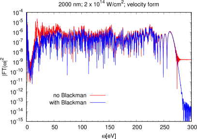
Figure 1: Harmonic spectrum of neon in a 2000 nm, $2.0\times 10^{14}\mbox{ W/cm}^{2}$ laser pulse, as obtained with RMT in the velocity form of the electric dipole operator with and without the Blackman window. The window generally reduces the result. The harmonic plateau extends from about 30 eV to a cutoff of about 260 eV.

After calculating the dipole expectation values, typically a Blackman window Blackman and Tukey (1959) is applied to ensure a smooth trend of both the dipole moment and its time derivative towards zero at the end of the pulse. Using the Blackman window significantly reduces the numerical noise arising from the Fourier transform needed to calculate the harmonic spectrum, and also improves the visibility of the cutoff. On the other hand, for short pulses where the dipole moment does not exhibit sufficient repetition, the window severely affects the absolute value of the spectral density, as shown in Fig. 1. The reduction in the absolute values is particularly evident at the beginning of the “plateau” from about $20-50$ eV, where it can exceed an order of magnitude and will severely affect the integral under the curve. Since we are interested in obtaining a quantitative value for the conversion efficiency, which is practically independent of both the steepness of the cutoff and the depth of the minimum in the spectral density at very low energies, we do not use this window in the present work.

Finally, we address the issue of which form is most appropriate to show the obtained spectra. For the SAE calculations, using the acceleration form after differentiating the induced dipole moment twice with respect to time provides the numerically cleanest results. The velocity form gives very similar results, except for the cutoff not being as deep and small changes in the depth of the low-energy minimum. Using the length form as written in Eq. (3), however, is problematic, as mentioned above. Indeed, a window like that used in the RMT code to limit the integration range for the calculation of the dipole moment fixes this problem, but it is not necessary when using the acceleration (or velocity) forms.

The RMT predictions obtained in both the length and velocity form directly give very similar results, as long as a window is used when the dipole moment is generated. As discussed by Baggesen and Madsen Baggesen and Madsen (2011), from a quantum-mechanical point of view, the velocity form might be the most natural one. Hence, most of the RMT calculations presented below were obtained directly with the matrix elements calculated in that form. The small price to pay is the less steep drop in the spectral density at the cutoff frequency, which however has practically no effect on the integral under the curve taken up to or even slightly above the cutoff.

As seen from the above discussion, a quantitative calculation of the spectral density, which is needed to obtain the conversion efficiency, is significantly more challenging than a purely qualitative description. All implementations we employed, be it SAE with a local potential or RMT with either one or two coupled channels, with simple or more sophisticated target wavefunctions, will predict a dominant peak in $S(\omega)$ at almost the driving frequency. This peak is followed by a deep minimum after about the fifth harmonic in our cases, a plateau, and finally a cutoff near the energy predicted by the three-step model Corkum (1993).

III Results and Discussion

The first step in determining the efficacy of RMT in producing water-window harmonics is to ensure that the length and velocity forms of the produced spectrum agree reasonably well.

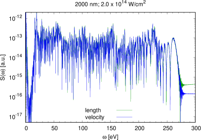
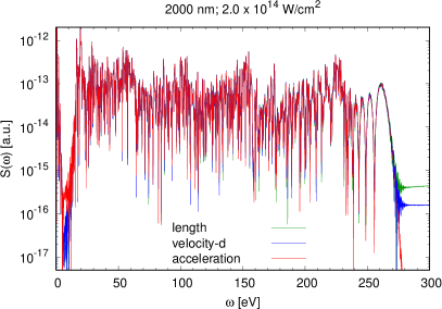
Figure 2: Harmonic spectrum of neon in a 2000 nm, $2.0\times 10^{14}\mbox{ W/cm}^{2}$ laser pulse. The top graph shows the RMT results obtained directly with the length and velocity matrix elements of the dipole operator, with the latter dropping off more after the cut-off. The bottom part shows the results obtained from the matrix elements in the length form (highest after the cut-off) and then the induced dipole moment differentiated (“-d”) once to get the velocity (middle line after the cut-off) and acceleration results (deepest after the cut-off). See text for details.

Figure 2 depicts a typical spectrum obtained in five different ways. Specifically, we compare the independent RMT results obtained with dipole matrix elements generated by RMATRX-II in the length and velocity gauges (top part of Fig. 2) and those obtained by differentiation of the dipole moment in the length form (bottom part). Except for the steepness of the cutoff and the depth of the low-frequency minimum, all the results are very similar and almost indistinguishable on the graph.

Figure 3: Harmonic spectrum neon in a 2000 nm, $2.0\times 10^{14}\mbox{ W/cm}^{2}$ laser pulse obtained with different values of $L_{\mathrm{max}}$.

Due to the large angular-momentum expansion needed for the calculation of multi-electron effects, it is also important to verify that the chosen value of the largest term ($L_{\mathrm{max}}$) does not affect the convergence of the results. This test is performed by running several calculations while increasing $L_{\mathrm{max}}$. A converged calculation is shown in Fig. 3, where the results obtained with values of $L_{\mathrm{max}}=200$ and $L_{\mathrm{max}}=240$ are very similar, while differences with those obtained with $L_{\mathrm{max}}=160$ are still visible.

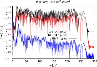
Figure 4: Harmonic spectrum of neon in a 2000 nm laser pulse with a peak intensity of $2.0\times 10^{14}\mbox{ W/cm}^{2}$, as obtained in the 1st-1cf RMT and SAE models. For the latter, the results for $m=0$ and $m=1$ are shown with the appropriate weighting factors. See text for details.

Having verified that the RMT calculations are both gauge-invariant and partial-wave converged, we can now investigate the results obtained using the SAE and RMT methods, as well as the trends when varying the physical parameters of the calculations. Figure 4 shows a comparison of SAE and RMT results for a wavelength of 2000 nm and a peak intensity of $2.0\times 10^{14}\mbox{ W/cm}^{2}$. We notice good qualitative agreement between the two sets of predictions. However, there are substantial differences in the details, especially in light of the logarithmic scale. As mentioned above, the SAE results need to be weighted by the initial magnetic quantum number of the $2p$ orbital. However, the figure shows that the contributions from $m=\pm 1$ are negligible compared to that from $m=0$. We also see that both sets of results (RMT and SAE for $m=0$) show the plateau reaching up to about 260 eV, in excellent agreement with the prediction of 258 eV from the three-step model.

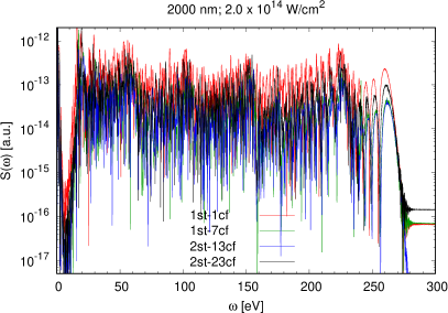
Figure 5: Harmonic spectrum of neon in a 2000 nm laser pulse with a peak intensity of $2.0\times 10^{14}\mbox{ W/cm}^{2}$. The results were obtained in the four RMT models described in the text.

In light of the differences seen between the SAE results and those from the simplest RMT model, i.e., 1st-1cf with the final ionic state described by only its dominant configuration in the expansion, we now investigate the sensitivity of the results on the number of coupled ionic states and their description. Our findings are shown in Fig. 5. While the qualitative predictions are practically identical, the quantitative results are not.

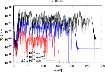
Figure 6: Harmonic spectra of neon in a 2000 nm laser pulse with peak intensities between $1.6\times 10^{14}\mbox{ W/cm}^{2}$ and $2.0\times 10^{14}\mbox{ W/cm}^{2}$. The harmonic cutoffs range from about 140 eV to 260 eV, following an approximately linear increase with intensity.

Since our principal goal is to test the RMT model, we now move to a discussion of the RMT results as a function of various experimentally controllable parameters. Figure 6 shows that the harmonic cutoff changes approximately linearly with intensity, as expected from Eq. (2). Furthermore, the calculated harmonic cutoffs agree well with those expected from Eq. (1). The largest disagreement is about 5 eV for the calculation with an intensity of $2.0\times 10^{14}\mbox{ W/cm}^{2}$.

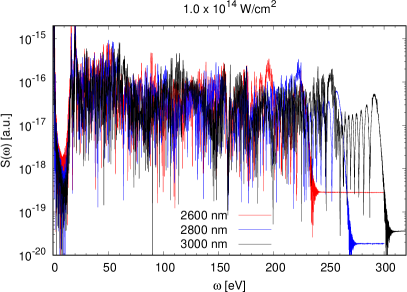
Figure 7: Harmonic spectra of neon in a $1.0\times 10^{14}\mbox{ W/cm}^{2}$ laser pulse with wavelengths ranging from 2600 nm to 3000 nm. As expected, the harmonic cutoffs vary from $\approx 220$ eV to $\approx 290$ eV.

Another expected trend based on Eq. (2) is an approximately quadratic increase in the harmonic cutoff with increasing wavelength. The cutoffs in Fig. 7, in general, agree with this expectation, with discrepancies of up to a few eV. This is not unexpected, as Eq. (2) does not account for the pulse envelope.

Though the calculations shown so far exhibit the characteristics expected from Eqs. (1) and (2), the cutoffs are not yet sufficiently high to reach into the water window. As shown in Fig. 8, increasing the wavelength to 3000 nm with a peak intensity of $1.5\times 10^{14}\mbox{ W/cm}^{2}$ finally pushes the cutoff into this window.

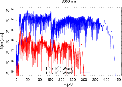
Figure 8: Harmonic spectra of neon from a 3000 nm pulse with peak intensities of $1.0\times 10^{14}\mbox{ W/cm}^{2}$ and $1.5\times 10^{14}\mbox{ W/cm}^{2}$. The latter produces a cutoff at $\approx 420$ eV.

Table 1: Conversion efficiency in the various models. $C_{t}$ is obtained by integrating over the entire spectrum until just above the cutoff, while the integration is limited to the plateau region for $C_{p}$.

Model	$\lambda$	Peak Intensity	$C_{t}$	$C_{p}$
SAE ($m=0$)	2000 nm	$2.0\times 10^{14}\mbox{ W/cm}^{2}$	$3.50\text{\times}{10}^{-3}$	$3.30\text{\times}{10}^{-3}$
SAE ($m=1$)	2000 nm	$2.0\times 10^{14}\mbox{ W/cm}^{2}$	$3.00\text{\times}{10}^{-4}$	$3.84\text{\times}{10}^{-9}$
1st-1cf	2000 nm	$2.0\times 10^{14}\mbox{ W/cm}^{2}$	$4.20\text{\times}{10}^{-2}$	$2.65\text{\times}{10}^{-2}$
1st-7cf	2000 nm	$2.0\times 10^{14}\mbox{ W/cm}^{2}$	$2.27\text{\times}{10}^{-2}$	$6.80\text{\times}{10}^{-3}$
2st-13cf	2000 nm	$2.0\times 10^{14}\mbox{ W/cm}^{2}$	$2.07\text{\times}{10}^{-2}$	$5.50\text{\times}{10}^{-3}$
2st-23cf	2000 nm	$2.0\times 10^{14}\mbox{ W/cm}^{2}$	$3.02\text{\times}{10}^{-2}$	$1.29\text{\times}{10}^{-2}$
2st-23cf	2000 nm	$1.5\times 10^{14}\mbox{ W/cm}^{2}$	$1.86\text{\times}{10}^{-2}$	$1.70\text{\times}{10}^{-3}$
2st-23cf	2000 nm	$1.0\times 10^{14}\mbox{ W/cm}^{2}$	$1.77\text{\times}{10}^{-2}$	$4.83\text{\times}{10}^{-5}$
2st-23cf	2600 nm	$1.0\times 10^{14}\mbox{ W/cm}^{2}$	$6.20\text{\times}{10}^{-3}$	$2.21\text{\times}{10}^{-5}$
2st-23cf	2800 nm	$1.0\times 10^{14}\mbox{ W/cm}^{2}$	$4.30\text{\times}{10}^{-3}$	$1.69\text{\times}{10}^{-5}$
2st-23cf	3000 nm	$1.0\times 10^{14}\mbox{ W/cm}^{2}$	$3.30\text{\times}{10}^{-3}$	$1.54\text{\times}{10}^{-5}$
2st-23cf	3000 nm	$1.5\times 10^{14}\mbox{ W/cm}^{2}$	$6.00\text{\times}{10}^{-3}$	$2.70\text{\times}{10}^{-3}$

We finish our presentation with the conversion efficiencies obtained in the various models and choices of parameters. These are listed in Table 1. As seen in the table, the predicted conversion efficiency depends significantly on the details of the model employed. In particular, the SAE results for 2000 nm at $2.0\times 10^{14}\mbox{ W/cm}^{2}$ are much smaller than those obtained with the more correlated RMT models. Even within the latter models, however, the predicted conversion efficiency $C_{p}$, obtained by integrating over the plateau region, varies between a minimum of $5.50\times 10^{-3}$ in 2st-13cf and a maximum of $2.65\times 10^{-2}$ in 1st-1cf. The variability is less in $C_{t}$, which is obtained by integrating over the entire spectrum. Apparently the models are less sensitive when it comes to predicting the dominant first peak near the driving frequency. This is the usual scenario that relatively large numbers are less affected by details in the model.

Next, it is important to investigate how the harmonic yield depends on the intensity and wavelength of the laser. As mentioned above, we expect the yield to decrease as the wavelength increases for fixed intensity. This expectation is somewhat indicated in Fig. 7 and clearly confirmed in Tab. 1. Specifically, increasing the wavelength from 2600 nm to 3000 nm at $2.0\times 10^{14}\mbox{ W/cm}^{2}$ reduces the total conversion efficiency $C_{t}$ by almost a factor of 2, which is consistent with an approximate $\lambda^{-5}$ dependence. However, the conversion efficiency $C_{p}$ at 3000 nm is still about 70% of the value at 2600 nm, thus suggesting a smaller reduction.

IV Conclusions and Outlook

We have investigated the efficacy of the $R$-Matrix with Time-dependence (RMT) method to generate high-order harmonics in the water window using mid-IR laser light. Previous approaches relied on significant simplifications that neglect both quantum-mechanical and multi-electron effects on the predicted spectra. Since it is not clear how accurate the results of these simplified models are, the present project was designed to carry out a thorough test.

We successfully demonstrated that RMT is capable of generating harmonics in the water window. We found qualitative agreement with the trends predicted in classical models and SAE calculations regarding the overall frequency dependence of the spectral density, specifically the dominating first few harmonics, the low-energy minimum, the plateau-like structure, and the cutoff frequency.

However, we found a significant dependence of the absolute values of the spectral density, and consequently the calculated conversion efficiency, on the details of the model employed. While employing windowing functions such as the Blackman window may improve the appearance of the spectrum, they significantly modify the shape of the harmonic plateau and therefore also the conversion efficiency, especially in few-cycle laser fields that are strongly ramped. Although it may seem unsatisfactory that we can only suggest that the results from our largest model (2st-23cf) are the most reliable, we hope that the detailed analysis provided in this paper will encourage further work and, in particular, motivate theorists to publish absolute numbers.

In the future, we plan to interface the RMT approach with the B-spline R-matrix (BSR) code of Zatsarinny Zatsarinny (2006), which allows the use of nonorthogonal, term-dependent target orbitals. As demonstrated in numerous applications to time-independent treatment of electron and photon collisions, we expect this to further improve the inner-region part of RMT, especially for complex targets. As an ultimate test of the RMT method, we hope to compare our predictions with experimental data. This will likely require substantial efforts by both the experimental and the theoretical communities. We hope that the work presented in this paper will stimulate such efforts.

References

- Neutze et al. (2000) R. Neutze, R. Wouts, D. van der Spoel, E. Weckert, and J. Hajdu, Nature 406, 752 (2000).
- Ackermann et al. (2007) W. Ackermann et al., Nat. Phot. 1, 336 (2007).
- Fu et al. (2020a) Y. Fu, K. Nishimura, R. Shao, A. Suda, K. Midorikawa, P. Lan, and E. J. Takahashi, Commun. Phys. 3, 92 (2020a).
- Rothhardt et al. (2014) J. Rothhardt, S. Hädrich, A. Klenke, S. Demmler, A. Hoffmann, T. Gotschall, T. Eidam, M. Krebs, J. Limpert, and A. Tünnermann, Opt. Lett. 39, 5224 (2014).
- Stein et al. (2016) G. J. Stein, P. D. Keathley, P. Krogen, H. Liang, J. P. Siqueira, C.-L. Chang, C.-J. Lai, K.-H. Hong, G. M. Laurent, and F. X. Kärtner, J. Phys. B: At. Mol. Opt. Phys. 49, 155601 (2016).
- Li et al. (2017) J. Li, X. Ren, Y. Yin, K. Zhao, A. Chew, Y. Cheng, E. Cunningham, Y. Wang, S. Hu, Y. Wu, et al., Nat. Commun. 8, 186 (2017).
- Fu et al. (2020b) Y. Fu, K. Nishimura, R. Shao, A. Suda, K. Midorikawa, P. Lan, and E. J. Takahashi, Commun. Phys. 3, 92 (2020b).
- Corkum (1993) P. B. Corkum, Phys. Rev. Lett. 71, 1994 (1993).
- Shiner et al. (2009) A. D. Shiner, C. Trallero-Herrero, N. Kajumba, H.-C. Bandulet, D. Comtois, F. Légaré, M. Giguère, J.-C. Kieffer, P. B. Corkum, and D. M. Villeneuve, Phys. Rev. Lett. 103, 073902 (2009).
- Lan et al. (2010) P. Lan, E. J. Takahashi, and K. Midorikawa, Phys. Rev. A 81, 061802 (2010).
- Jin et al. (2014) C. Jin, G. Wang, H. Wei, A.-T. Le, and C. D. Lin, Nat. Commun. 5, 4003 (2014).
- Teichmann et al. (2016) S. M. Teichmann, F. Silva, S. L. Cousin, M. Hemmer, and J. Biegert, Nat. Commun. 7, 11493 (2016).
- Ishii et al. (2014) N. Ishii, K. Kaneshima, K. Kitano, T. Kanai, S. Watanabe, and J. Itatani, Nat. Commun. 5, 3331 (2014).
- Nishimura et al. (2021) K. Nishimura, Y. Fu, A. Suda, K. Midorikawa, and E. J. Takahashi, Rev. Sci. Instr. 92, 063001 (2021).
- Lewenstein et al. (1994) M. Lewenstein, P. Balcou, M. Y. Ivanov, A. L’Huillier, and P. B. Corkum, Phys. Rev. A. 49, 2117 (1994).
- Ivanov and Kheifets (2009) I. A. Ivanov and A. S. Kheifets, Phys. Rev. A 79, 053827 (2009).
- Mazza et al. (2015) T. Mazza, A. Karamatskou, M. Ilchen, S. Bakhtiarzadeh, A. J. Rafipoor, P. O’Keeffe, T. J. Kelly, N. Walsh, J. T. Costello, M. Meyer, et al., Nat. Commun. 6, 6799 (2015).
- Gordon et al. (2006) A. Gordon, F. X. Kärtner, N. Rohringer, and R. Santra, Phys. Rev. Lett. 96, 223902 (2006).
- Miyagi and Madsen (2013) H. Miyagi and L. B. Madsen, Phys. Rev. A 87, 062511 (2013).
- Sato et al. (2016) T. Sato, K. L. Ishikawa, I. Březinová, F. Lackner, S. Nagele, and J. Burgdörfer, Phys. Rev. A 94, 023405 (2016).
- Tikhomirov et al. (2017) I. Tikhomirov, T. Sato, and K. L. Ishikawa, Phys. Rev. Lett. 118, 203202 (2017).
- Artemyev et al. (2017) A. N. Artemyev, L. S. Cederbaum, and P. V. Demekhin, Phys. Rev. A 95, 033402 (2017).
- Woźniak et al. (2022) A. P. Woźniak, M. Przybytek, M. Lewenstein, and R. Moszyński, J. Chem. Phys. 156, 174106 (2022).
- Kutscher et al. (2022) E. Kutscher, A. N. Artemyev, and P. V. Demekhin, Frontiers in Chemistry 10 (2022).
- Brown et al. (2020) A. C. Brown, G. S. Armstrong, J. Benda, D. D. Clarke, J. Wragg, K. R. Hamilton, Z. Mašín, J. D. Gorfinkiel, and H. W. van der Hart, Comp. Phys. Commun. 250, 107062 (2020).
- Hassouneh et al. (2014) O. Hassouneh, A. C. Brown, and H. W. van der Hart, Phys. Rev. A 90, 043418 (2014).
- Pauly et al. (2020) T. Pauly, A. Bondy, K. R. Hamilton, N. Douguet, X.-M. Tong, D. Chetty, and K. Bartschat, Phys. Rev. A 102, 013116 (2020).
- Tong and Lin (2005) X. M. Tong and C. D. Lin, J. Phys. B: At. Mol. Opt. Phys. 38, 2593 (2005).
- Joachain et al. (2012) C. J. Joachain, N. Kylstra, and R. M. Potvliege, Atoms in Intense Laser Fields (Cambridge University Press, 2012).
- Telnov et al. (2013) D. A. Telnov, K. E. Sosnova, E. Rozenbaum, and S.-I. Chu, Phys. Rev. A 87, 053406 (2013).
- Moore et al. (2011) L. R. Moore, M. A. Lysaght, L. A. Nikolopoulos, J. S. Parker, H. W. van der Hart, and K. T. Taylor, J. Mod. Optics 58, 1132 (2011).
- Hutchinson et al. (2010) S. Hutchinson, M. A. Lysaght, and H. W. van der Hart, J. Phys. B: At. Mol. Opt. Phys. 43, 095603 (2010).
- Cormier and Lambropoulos (1996) E. Cormier and P. Lambropoulos, J. Phys. B: At. Mol. Opt. Phys. 29, 1667 (1996).
- Grum-Grzhimailo et al. (2010) A. N. Grum-Grzhimailo, B. Abeln, K. Bartschat, D. Weflen, and T. Urness, Phys. Rev. A 81, 043408 (2010).
- Burke and Taylor (1975) P. G. Burke and K. T. Taylor, J. Phys. B: At. Mol. Phys. 8, 2620 (1975).
- (36) https://gitlab.com/Uk-amor/RMT/rmatrixII.
- Brown et al. (2012) A. C. Brown, D. J. Robinson, and H. W. van der Hart, Phys. Rev. A 86, 053420 (2012).
- Hamilton et al. (2017) K. R. Hamilton, H. W. van der Hart, and A. C. Brown, Phys. Rev. A 95, 013408 (2017).
- Gaumnitz et al. (2017) T. Gaumnitz, A. Jain, Y. Pertot, M. Huppert, I. Jordan, F. Ardana-Lamas, and H. J. Wörner, Opt. Express 25, 27506 (2017).
- Ivanov et al. (2014) I. A. Ivanov, A. S. Kheifets, K. Bartschat, J. Emmons, S. M. Buczek, E. V. Gryzlova, and A. N. Grum-Grzhimailo, Phys. Rev. A 90, 043401 (2014).
- (41) https://www.tacc.utexas.edu/systems/stampede2.
- (42) https://www.tacc.utexas.edu/systems/frontera.
- (43) https://www.psc.edu/resources/bridges-2.
- Blackman and Tukey (1959) R. B. Blackman and J. W. Tukey, The Measurement of Power Spectra: From the Point of View of Communications Engineering (Dover, 1959), pp. 98–99.
- Baggesen and Madsen (2011) J. C. Baggesen and L. B. Madsen, J. Phys. B: At. Mol. Phys. 44, 115601 (2011).
- Zatsarinny (2006) O. Zatsarinny, Comp. Phys. Commun. 174, 273 (2006).
- (47) https://www.ukamor.com/#/software.