Comparison of Minimization Methods for Rosenbrock Functions

Abstract

This paper gives an in-depth review of the most common iterative methods for unconstrained optimization using two functions that belong to a class of Rosenbrock functions as a performance test. This study covers the Steepest Gradient Descent Method, the Newton-Raphson Method, and the Fletcher-Reeves Conjugate Gradient method. In addition, four different step-size selecting methods including fixed-step-size, variable step-size, quadratic-fit, and golden section method were considered. Due to the computational nature of solving minimization problems, testing the algorithms is an essential part of this paper. Therefore, an extensive set of numerical test results is also provided to present an insightful and a comprehensive comparison of the reviewed algorithms. This study highlights the differences and the trade-offs involved in comparing these algorithms.

I Introduction

Solutions to unconstrained optimization problems can be applied to multi-agent systems and machine learning problems, especially if the problem is in a decentralized or distributed fashion [1], [2], [3] and [4]. Sometimes, in adversarial attack applications, malicious agents can be present in a network that will slow down convergence rates to optimal points as seen in [5], [6] and [7]. Therefore the need for a fast convergence and cost associated with it are usually necessities by recent researchers. The steepest descent method is a good first order method for obtaining optimal solutions if an appropriate step size is chosen. Some methods of choosing step sizes include the fixed step size, the variable step size, the polynomial fit, and the golden section method that will be discussed in details in subsequent sections. Nonetheless, these methods have their own merits and demerits. A second order method such as the Newton-Raphson method is very suitable for quadratic problems and attains optimality in a small number of iterations [8]. However the Newton-Raphson method requires computing the Hessian and its inverse which are often a bottleneck. For this reason, the Newton-Raphson method may not be suitable for solving large scale optimization problems.

To address the lapses that the Newton-Raphson method poses, some methods have been recently proposed such as matrix splitting discussed in [9]. Another way of obtaining fast convergence properties of second-order methods using the structure of first-order methods are the Quasi-Newton methods. These methods incorporate second-order (curvature information) in the first-order approaches. Examples of these methods include the Broyden-Fletcher-Goldfarb-Shanno algorithm (BFGS) [10] and the Barzilai-Borwein (BB) [11] and [12]. However these methods usually require additional assumptions on the objective function to be minimized to be strongly convex and that the gradient of such function to be Lipschitz continuous to improve convergence rate discussed in [13]. The conjugate gradient method [14] on the other hand does not have as much restrictions as the Newton-Raphson method in terms of computing the inverse of the Hessian. The method computes the direction of search at each iteration and the direction is expressed as a linear combination of previous search direction calculation and the present gradient at the present iteration. The other interesting attribute of the conjugate gradient method is that it gives different methods of calculating the search directions and it is not only limited to quadratic functions as we will use that while performing simulations using the Rosenbrock function [8].

The crux of our work entails comparing the convergence properties of first order and second order methods and the limitations of each method using two Rosenbrock functions. One of the two functions is usually known as the banana function and is much more difficult to minimize than the other. We compare convergence attributes for these methods by examining these Rosenbrock functions where one is a alteration of the other. The first order type methods we used for this study include the steepest descent with fixed step size, variable step size, polynomial quadratic fit and golden section method. For the second order method, we consider the Newton-Raphson method and compare its performance with the Conjugate Gradient Methods. The above methods highlighted have their own advantages and disadvantages in terms of general performance, convergence, precision, convergence rate, and robustness. Depending upon the nature of the problem, performance design specifications, and available resources, one can select the most appropriate optimization method. In order to assist this effort, this study will highlight the differences and the trade-offs involved in comparing these algorithms.

I-A Contributions

In this paper, we compare different types of methods as described to analyse convergence without restricting the analysis to quadratic functions. As we will see in subsequent sections, we examined first order methods using four different cases like the fixed step size, variable step size, quadratic fit and the golden section methods. In our analysis, we did not depend on the steepest descent with fixed step size commonly used by many researchers to study first order methods. This paper also compares second order methods and highlights the advantages the Newton-Raphson and conjugate gradient methods have over each other.

I-B Paper Pattern

Section II presents the problem formulation, section introduces the different types of first and second type methods, and their convergence analysis. Numerical experiments are performed in section IV and the conclusion is given in section V.

I-C Notation

We denote the set of positive and negative reals as $\mathbb{R}_{+}$ and $\mathbb{R}_{-}$, the transpose of a vector or matrix as $(\cdot)^{T}$, and the L$2$-norm of a vector by $||\cdot||$. We let the gradient of a function $f(\cdot)$ to be $\nabla f(\cdot)$, the Hessian of a function $f(\cdot)$ be $F(\cdot)=\nabla^{2}f(\cdot)$, and $\langle\ \cdot,\cdot\rangle$ denotes the inner product of two vectors.

II Problem formulation

In mathematical optimization, Rosenbrock functions are used as a performance test problem for optimization algorithms [15]. So we will use the following Rosenbrock functions in our analysis.

$$\underset{x_{1},x_{2}}{\operatorname{minimize}} f(x_{1},x_{2})=\kappa(x_{1}^{2}-x_{2})^{2}+(x_{1}-1)^{2}$$ (1)

where $\kappa>0$, $x$ is a vector such that $x=[x_{1},x_{2}]^{T}$ and $f(x)$ in problem (1) is strictly convex and twice differentiable.. We will examine the key role $\kappa$ plays in affecting convergence in section IV. To solve the minimization problems (1) using gradient methods, we let the iterative equation generated by the minimization problem (1) be given by:

$$x(k+1)=x(k)-\alpha(k)\nabla f(x(k)),$$ (2)

where $k$ is the iteration, $\alpha(k)>0$ is the step size and $\nabla f(x(k))$ is the gradients of $f$ at each iterate $x(k)$. Different first order and second order methods for solving problem (1) will be explored in the later part of the paper.

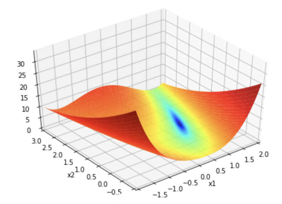
Figure 1: Surface plot for function (1) over $\mathbb{R}^{2}$ when $\kappa=1$

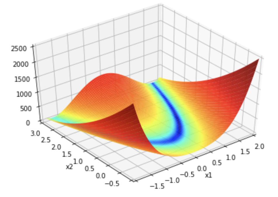
Figure 2: Surface plot for function (1) over $\mathbb{R}^{2}$ when $\kappa=100$

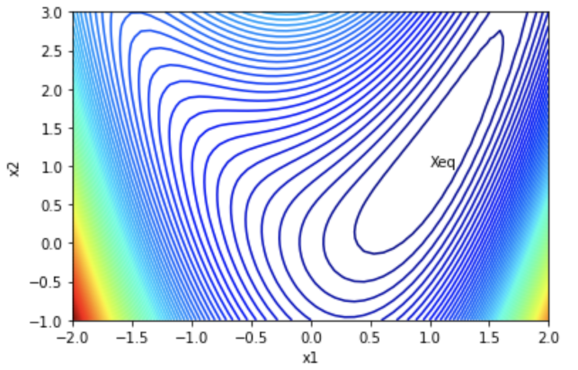
Figure 3: Level curves for function (1) over $\mathbb{R}^{2}$ when $\kappa=1$

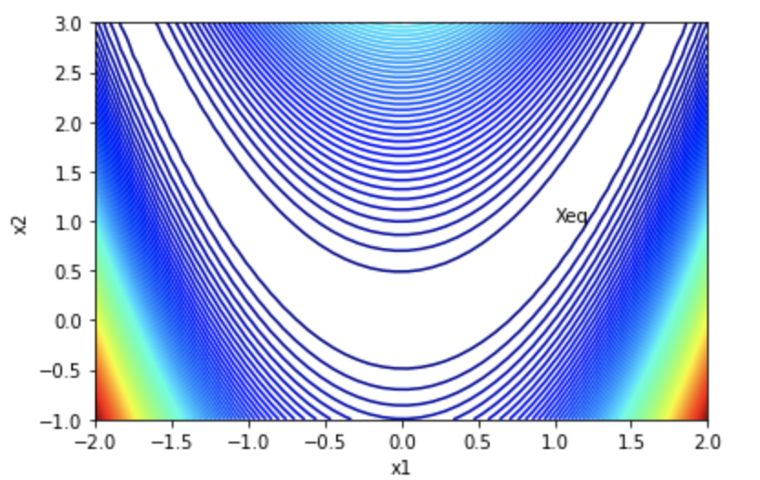
Figure 4: Level curves for function (1) over $\mathbb{R}^{2}$ when $\kappa=100$

The level curves for function 1 with $\kappa=1$ and $\kappa=100$ are shown in Fig. 3 and Fig. 4 respectively. Even though $f(x)$ has a global minimum at $(1,1)$, the global minimum of $f(x)$ when $\kappa=100$ is inside a longer blue parabolic shaped flat valley than it is when $\kappa=1$ as shown in Fig. 1 and Fig. 2. Due to the longer size of the valley in Fig. 2, attaining convergence to the minimum of $f(x)$ with $\kappa=100$ becomes increasingly difficult. As such, the functions generated by (1) with $\kappa=1$ and $\kappa=100$ are excellent candidates to evaluate the characteristics of optimization algorithms, such as: convergence rate, precision, robustness, and general performance. In this paper, function (1) with $\kappa=1$ and $\kappa=100$ will be employed to establish a numerical comparison of the three optimization algorithms discussed below in section III.

III Analysis of First and Second order methods

We now discuss the most common iterative methods for unconstrained optimization.

III-A The Steepest Descent Method

To solve problem (1), a sequence of guesses $x(0),x(1),...x(k),x(k+1)$ will be generated in a descent manner such that $f(x(0))>f(x(1))>...>f(x(k+1))$. It can be often tedious to obtain optimality after some $K$ iterations, and $K$ is the maximum number of iterations needed for convergence such that $\nabla f(x(K))=0$. Therefore it suffices to actually modify the gradient stopping condition to satisfy $\|\nabla f(x(K))\|\leq\varepsilon$ where $\varepsilon>0$ and very small which is often referred to as the stopping criterion for convergence to hold. Different ways of choosing the step size will be explored below:

III-A1 Steepest Descent With a Constant Step Size

The constant step size is constructed in a manner where you simply use one value of $\alpha$ in all iterations. To illustrate the fixed step size principle in solving problem (1), we will pick an $\alpha$ value between $0$ and $1$ and show numerically how convergence is attained.

Other methods of choosing the step size in a steepest descent algorithm are discussed below:

III-A2 Steepest Descent with Variable Step Size

In the variable step size method, $3$ or $4$ values of $\alpha$ are chosen at each iteration and the value that produces the smallest $g(\alpha(k))$ value will be chosen where $g(\alpha(k))=f(x(k+1))$. The variable step size algorithm is also easy to implement and has a better convergence probability than the fixed step size method. The results of simulating problem (1) with $\kappa=1$ and $\kappa=100$ using the variable step size are shown in (IV).

III-A3 Steepest Descent with Quadratic Fit Method

For the quadratic fit method, three values of $\alpha(k)$ are guessed at each iteration and the values of the corresponding $g(\alpha(k))$ values are computed, where $g(\alpha(k))=f(x(k+1))$ For example, suppose the three values of $\alpha$ values chosen are $\alpha(1),\alpha(2),\alpha(3)$. To fit a quadratic model of the form:

$$g(\alpha)=a\alpha^{2}+b\alpha+c,$$ (3)

we write the quadratic model based on $\alpha$ values as:

$$g(\alpha(1))=a\alpha(1)^{2}+b\alpha(1)+c,$$ (4)

$$g(\alpha(2))=a\alpha(2)^{2}+b\alpha(2)+c,$$ (5)

$$g(\alpha(3))=a\alpha(3)^{2}+b\alpha(3)+c.$$ (6)

where $a,b,c$ are constants. After solving for $a,b,c$ in equations (4), (5), and (6), we will use these values in equation (3) to obtain the optimum step size which is the mimimum of equation (3).

III-A4 Steepest Descent with the Golden Section Search

In this algorithm, we use a range between two values and divide the range into sections. We then eliminate some sections within the sections in the range to shrink the region where the convergence might occur. For this algorithm to be implemented as we will see in section (IV), the initial region of uncertainty and the stopping criterion have to be defined. An example where a golden section search was applied to minimize a function in a closed interval is seen in [8].

Second-order methods have been an improvement in terms of convergence speeds when it comes to solving unconstrained optimization problems such as problem (1). We will show by simulations in section IV the speed of convergence for the Newton-Raphson and conjugate gradient methods compared to other methods. We will now analyze the two second order methods below:

III-B Newton-Raphson Methods

The Newton-Raphson Method is very useful in obtaining fast convergence of an unconstrained problem like in equation (1) especially when the initial starting point is very close to the minimum. The main disadvantage of this method is the cost and difficulty associated with finding the inverse of the Hessian and also ensuring that the Hessian inverse matrix is positive definite. The update equation for the Newton-Raphson Method is given by:

$$x(k+1)=x(k)-F^{-1}(x(k)){\nabla f(x(k))}.$$ (7)

Some of the methods of approximating the term that contains the inverse of the Hessian, $F^{-1}(x(k))$ in equation (7) are the Quasi-Newton methods such as the BFGS and the Barzilai-Borwein methods [10], [16].

III-C Conjugate Gradient Methods

For the class of quadratic functions $f(x)=0.5x^{T}Qx-x^{T}b$, and $x\in\mathbb{R}^{n}$, the conjugate gradient algorithm uses a direction expressed in terms of the current gradient and the previous direction at each iteration by ensuring that the directions are mutually Q-conjugate, where $Q$ is a positive definite symmetric $n\times n$ matrix [14]. We note that the directions $d(0),d(1),.....d(m)$ are Q-conjugate if $d(i)^{T}Qd(j)=0$, and $i\neq j$. The conjugate gradient method also exhibits fast convergence property for non-quadratic problems like problem (1). In the simulation in section IV, we use the Fletcher-Reeves Formula [17] given by:

$$\beta(k)=\frac{g(k+1)^{T}g(k+1)}{g(k)^{T}g(k)}$$

where $g(k)=\nabla f(x(k))$ and $\beta(k)$ are constants picked such that the directional iteration $d(k+1)$ is Q-conjugate to $d(0),d(1),.....d(k)$ according to the following iterations:

$$x(k+1)=x(k)+\alpha(k)d(k),$$

and $\alpha(k)>0$ is the step size. We will show in section IV that the conjugate gradient method performs better than the steepest descent method in terms of convergence rate when we use the same fixed step size.

IV Numerical Experiments Insights

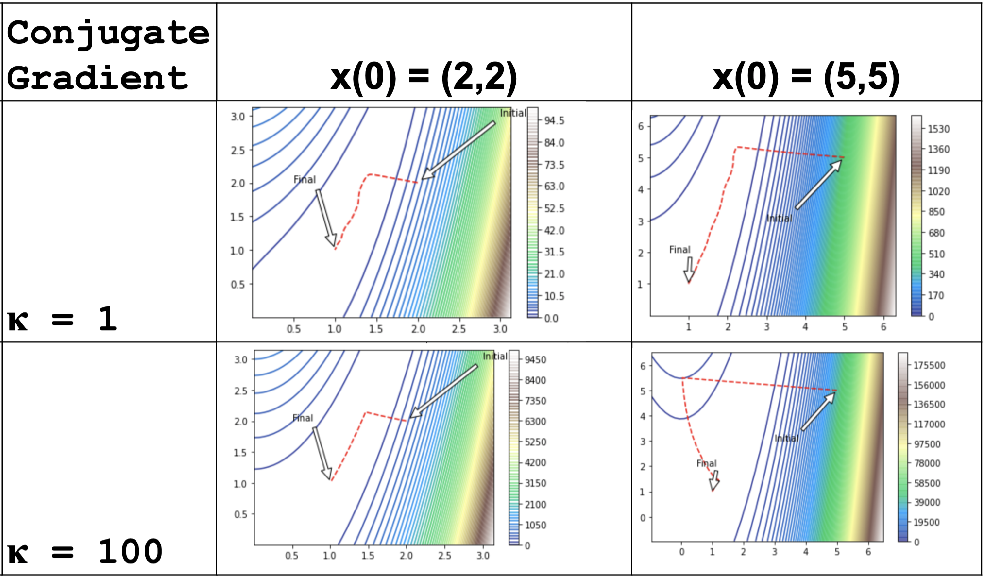
Figure 11: Level curves for Conjugate Gradient method.

In this section, we will compare the methods discussed in section III in terms of convergence and the number of iterations taken to reach optimality in problem (1) for cases when $\kappa=1$ and $\kappa=100$. For these two cases, initial conditions of $(2,2)$ and $(5,5)$ and a stopping criterion of $\|\nabla f(x(K))\|\leq 0.001$ are used across all these methods discussed where $K$ is the maximum iteration number to achieve convergence. Fig. 5 summarizes the numerical result whereas Fig. 6 - Fig 11 illustrate the trajectory of iterates $x(k)$ on level curves of the functions across all cases. The code for the experiments is available here.

IV-A Geometric Step Size Test

To compare the methods discussed in section III, a geometric sequence of fixed step sizes is used. We note that the Newton-Raphson method is not dependent on any step-size. As a result, the geometric step size test includes the the steepest descent and Conjugate Gradient Methods. Using the fixed step sizes, $0.124$, $0.0124$, $0.00124$ and $0.000124$, we present the results as follows.

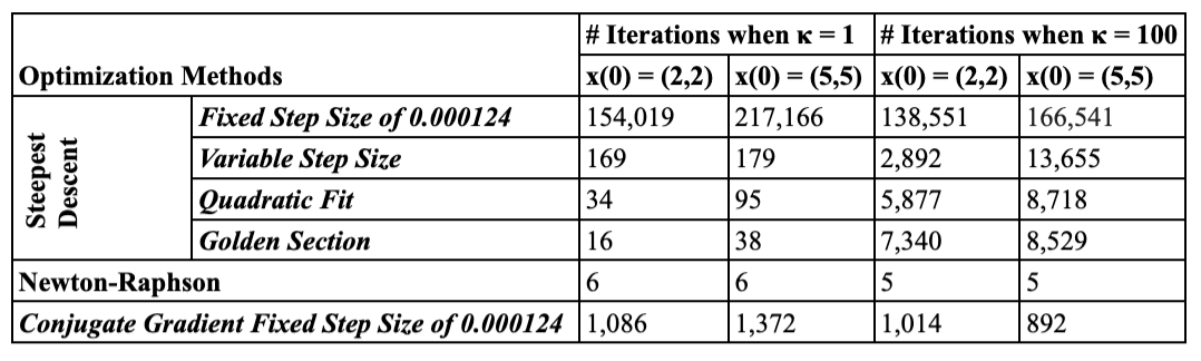
Figure 5: Numerical Comparison of the three optimization methods for the two functions with step-size = 0.000124

IV-A1 Case when $\alpha=0.124$

When $\kappa=1$ and the step size $\alpha=0.124$ is used, the minimization problem (1) generated by (2) converges for the steepest descent with the $(2,2)$ initial condition and diverges with the initial condition of $(5,5)$. Equation (2) also diverges with the conjugate gradient with both of the initial starting points.

When $\kappa=100$ and the step size $\alpha=0.124$ is used, the problem (1) generated by (2) diverges by the steepest descent for both initial points, and also diverges by the conjugate gradient using both initial points, $(2,2)$ and $(5,5)$.

IV-A2 Case when $\alpha=0.0124$

When $\kappa=1$, and the steepest descent method is applied on the function (1) generated by iteration (2), convergence is attained with both of the starting initial points. This is an improvement over the case when $\alpha=0.124$, where the steepest method diverges using the initial point $(5,5)$. By the conjugate method on function, convergence is obtained with both starting points which is also an improvement over the case when $\alpha=0.124$, where it diverges for both starting values.

For equation (1) generated by (2) when the step size $\alpha=0.0124$ is used with $\kappa=100$, there was no improvement in convergence attributes because divergence is obtained by steepest descent and conjugate gradient methods for both of the initial points.

IV-A3 Case when $\alpha=0.00124$

At the stage when $\alpha=0.00124$ is used, the conjugate-gradient and the steepest descent both converge with both starting points for function (1) generated by (2) with $\kappa=1$. By using equation (1) generated by (2) with $\kappa=100$ and $\alpha=0.00124$, convergence is obtained using the initial point $(2,2)$ compared to divergence result obtained by using the initial point $(5,5)$.

IV-A4 Case when $\alpha=0.000124$

When the step size $\alpha=0.000124$ is used, the steepest descent method and conjugate gradient method converge for equation (1) generated by (2) for both $\kappa=1$ and $\kappa=100$. In addition, for each function, we observed that for both initial points $(2,2)$ and $(5,5)$ result in convergence. Therefore we will use this step size as a case study to compare the rate of convergence of steepest descent and conjugate gradient for the two functions with the two starting points.

IV-B Significance of the Newton-Raphson Method

The significance of the Newton-Raphson method should not be overlooked even for non-quadratic functions like (1) because the method guarantees convergence to the optimal solution without specifying a step size. Moreover, it achieves convergence in just few iterations for both of the starting points as well as for the two functions. This affirms the unique convergence attribute of the Newton-Raphson method when the starting point is not far away from the optimal solution.

IV-C Comparison of the Variable Step Size, Quadratic Fit and Golden Section with other Methods

Starting with the two initial points $(2,2)$ and $(5,5)$ using the variable step size method, convergence was obtained for the function (1) for both cases $\kappa=1$ and $\kappa=100$ when three varying step sizes of $0.000124$, $0.0124$ and $0.124$ are used. When the quadratic fit is used, three values of the step sizes are used in each iteration and selected from the range $(0.00001,0.000124)$. The result from the quadratic fit shows that a better convergence is achieved for function (1) with $\kappa=1$ but shows a weaker convergence for the second function. This explains that fluctuations in the random selection of step sizes between a range can influence the convergence rate. Moreover, the alteration parameter $\kappa$ from function (1) can also slow down convergence rates. For the golden section method, a range of $(0.00000124,1.5)$ is used to locate the value of the step size that result in the solution to the minimization problem (1). By using the initial points of $(2,2)$ and $(5,5)$ on the function (1) with $\kappa=1$, the golden section method resulted in the fastest convergence rate by comparing with the steepest descent with fixed step size, variable step size and the quadratic fit methods. However, convergence with the golden section is faster than the variable, fixed step size and the quadratic fit methods when the same initial starting conditions are used for function (1) with $\kappa=100$.

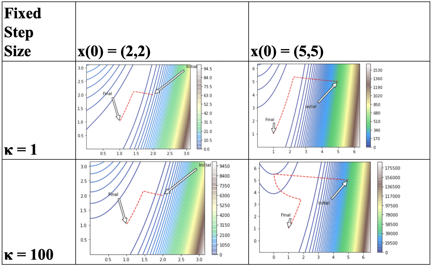
Figure 6: Level curves for Steepest Gradient Descent with fixed step size.

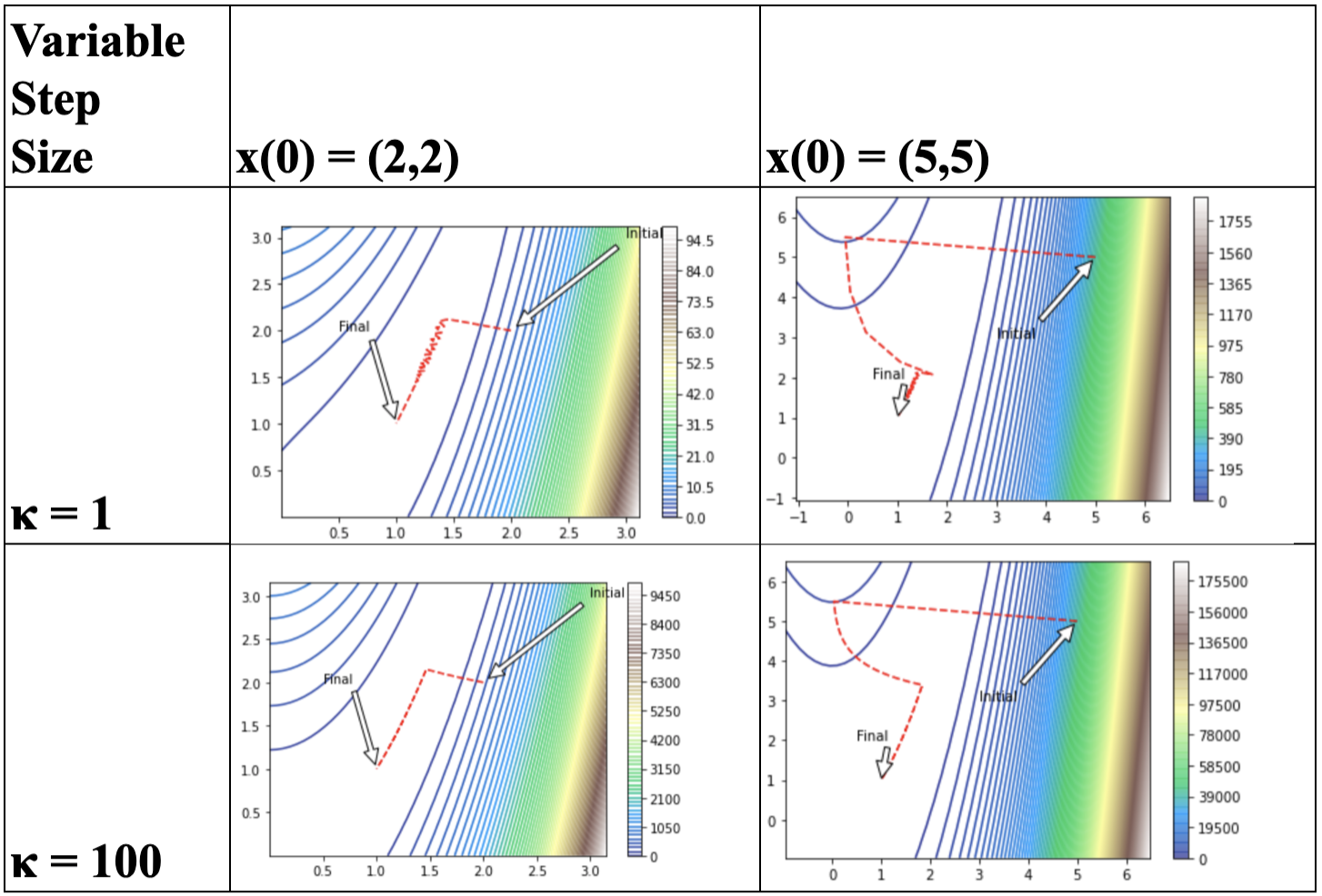
Figure 7: Level curves for Steepest Gradient Descent with variable step size.

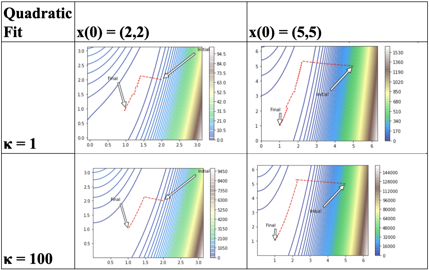
Figure 8: Level curves for Steepest Gradient Descent with quadratic fit.

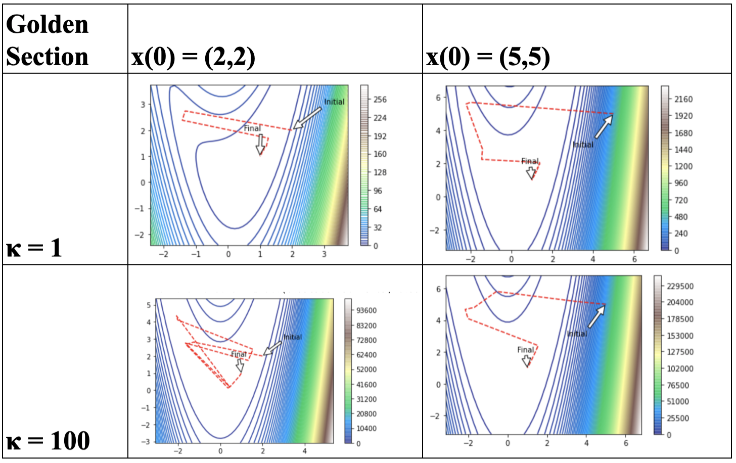
Figure 9: Level curves for Steepest Gradient Descent with golden section

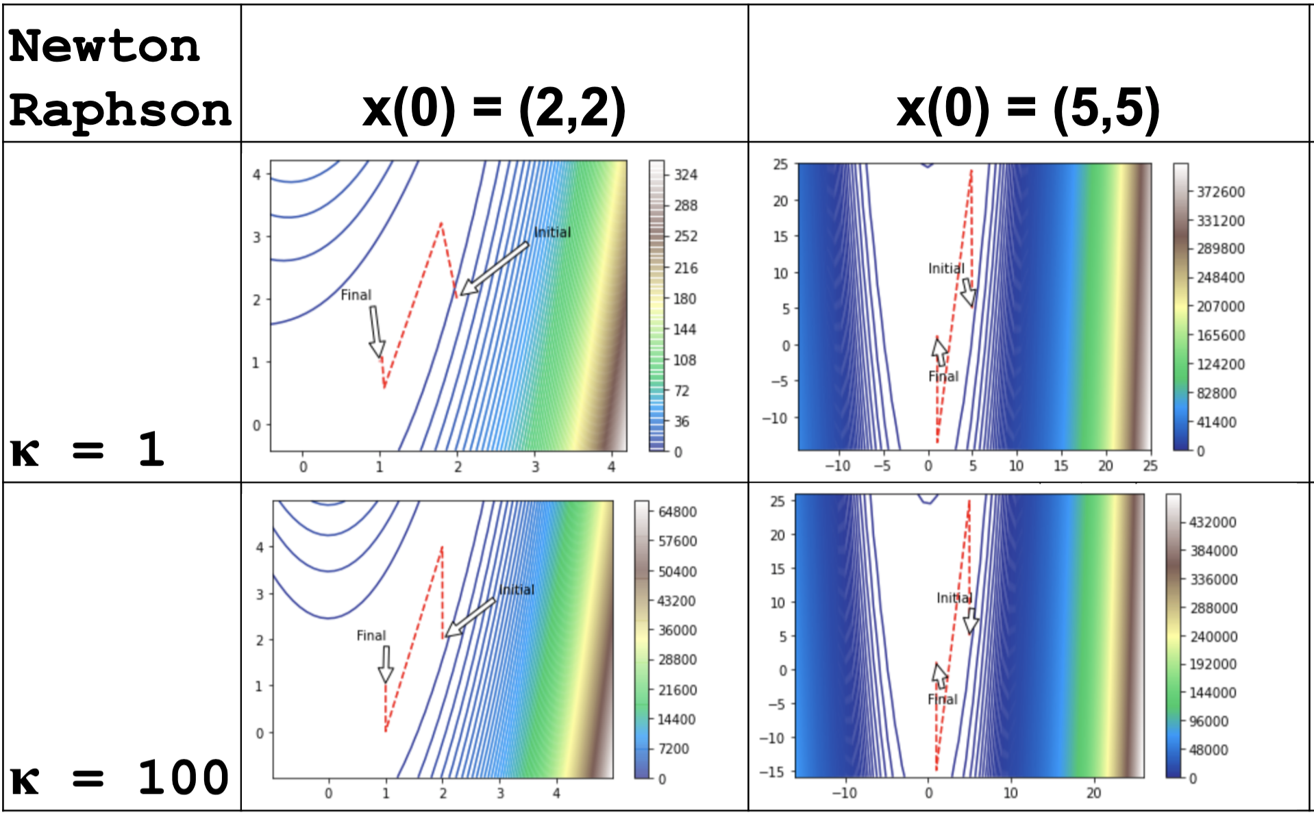
Figure 10: Level curves for Newton-Raphson’s method.

V Conclusions

We analyze convergence attributes of some selected first and second order methods such as the steepest descent, Newton-Raphson, and conjugate gradient and apply it to a class of Rosenbrock functions. We show through different minimization algorithms for function (1) using values $\kappa=1$ and $\kappa=100$ that it is still possible for equation (1) to converge to its minimum.Numerical experiments affirm that the Newton-Raphson method has the fastest convergence rate for the two strictly convex functions used in this paper provided the initial starting point is close to the minimum as seen with the starting points used. To conclude, choosing the best method depends on the type of problem, the performance design specifications, and the resources available. As such, this study highlighted the differences and the trade-offs involved in comparing these algorithms to contribute to one’s endeavor in selecting the most appropriate optimization method.

References

- [1] A. Nedić, A. Olshevsky, and M. G. Rabbat, “Network topology and communication-computation tradeoffs in decentralized optimization,” Proceedings of the IEEE, vol. 106, no. 5, pp. 953–976, 2018.
- [2] S. Yang, Q. Liu, and J. Wang, “Distributed optimization based on a multiagent system in the presence of communication delays,” IEEE Transactions on Systems, Man, and Cybernetics: Systems, vol. 47, no. 5, pp. 717–728, 2016.
- [3] E. Montijano and A. R. Mosteo, “Efficient multi-robot formations using distributed optimization,” in 53rd IEEE Conference on Decision and Control. IEEE, 2014, pp. 6167–6172.
- [4] K. I. Tsianos, S. Lawlor, and M. G. Rabbat, “Consensus-based distributed optimization: Practical issues and applications in large-scale machine learning,” in 2012 50th annual allerton conference on communication, control, and computing (allerton). IEEE, 2012, pp. 1543–1550.
- [5] I. Emiola, L. Njilla, and C. Enyioha, “On distributed optimization in the presence of malicious agents,” 2021.
- [6] S. Sundaram and B. Gharesifard, “Distributed optimization under adversarial nodes,” IEEE Transactions on Automatic Control, vol. 64, no. 3, pp. 1063–1076, 2018.
- [7] N. Ravi, A. Scaglione, and A. Nedić, “A case of distributed optimization in adversarial environment,” in ICASSP 2019-2019 IEEE International Conference on Acoustics, Speech and Signal Processing (ICASSP). IEEE, 2019, pp. 5252–5256.
- [8] E. K. Chong and S. H. Zak, An introduction to optimization. John Wiley & Sons, 2004.
- [9] M. Zargham, A. Ribeiro, A. Ozdaglar, and A. Jadbabaie, “Accelerated dual descent for network flow optimization,” IEEE Transactions on Automatic Control, vol. 59, no. 4, pp. 905–920, 2013.
- [10] M. Eisen, A. Mokhtari, and A. Ribeiro, “Decentralized quasi-newton methods,” IEEE Transactions on Signal Processing, vol. 65, no. 10, pp. 2613–2628, 2017.
- [11] Y.-H. Dai and R. Fletcher, “Projected barzilai-borwein methods for large-scale box-constrained quadratic programming,” Numerische Mathematik, vol. 100, no. 1, pp. 21–47, 2005.
- [12] P. E. Gill and W. Murray, “Quasi-newton methods for unconstrained optimization,” IMA Journal of Applied Mathematics, vol. 9, no. 1, pp. 91–108, 1972.
- [13] J. Gao, X. Liu, Y.-H. Dai, Y. Huang, and P. Yang, “Geometric convergence for distributed optimization with barzilai-borwein step sizes,” arXiv preprint arXiv:1907.07852, 2019.
- [14] M. R. Hestenes, E. Stiefel et al., Methods of conjugate gradients for solving linear systems. NBS Washington, DC, 1952, vol. 49, no. 1.
- [15] H. H. Rosenbrock, “An Automatic Method for Finding the Greatest or Least Value of a Function,” The Computer Journal, vol. 3, no. 3, pp. 175–184, 01 1960. [Online]. Available: https://doi.org/10.1093/comjnl/3.3.175
- [16] I. Emiola, “Sublinear regret with barzilai-borwein step sizes,” 2021.
- [17] R. Fletcher and C. M. Reeves, “Function minimization by conjugate gradients,” The computer journal, vol. 7, no. 2, pp. 149–154, 1964.