On the Higher Loop Euler-Heisenberg Trans-Series Structure

Abstract

We show that the one-loop Euler-Heisenberg QED effective Lagrangian in a constant background field acquires a very different non-perturbative trans-series structure at two-loop and higher-loop order in the fine structure constant. Beyond one-loop, virtual particles interact, causing fluctuations about the instantons, whereby the simple poles of the one-loop Borel transform become branch points. We illustrate this in detail at two-loop order using Ritus’s seminal result for the renormalized two-loop effective Lagrangian as an exact double-integral representation, and propose a possible new approach to computations at higher loop order. Our methods yield remarkably accurate extrapolations from weak-field to strong-field, and from magnetic to electric background field, at both one-loop and two-loop order, based on surprisingly little perturbative input.

I Introduction

The exact renormalized one-loop QED effective Lagrangian in a uniform background electromagnetic field was computed long ago by Euler and Heisenberg [1, 2, 3, 4, 5]. This computation is made possible by the existence of a simple exact integral representation of the electron propagator in a constant background field [6, 7]. When the constant background field is purely magnetic, the one-loop effective Lagrangian is real, but when the constant background field is electric, the one-loop effective Lagrangian has both a real and imaginary part. The non-perturbative imaginary part determines the rate of electron-positron pair-production from vacuum [1, 3]. The one-loop Euler-Heisenberg expression in [1] is an explicit Borel-Laplace integral representation, so the non-perturbative properties can be extracted straightforwardly from the singularity structure of the exact Borel transform function, which has only pole singularities. This meromorphic property of the Borel transform no longer holds at higher loop order. The two-loop Euler-Heisenberg effective Lagrangian, which includes the new effect of photon exchange between the virtual particles in the fermion loop (see Figure 1), was first calculated by Ritus [8, 9, 10, 11], also based on the exact proper-time integral representation of the electron propagator. A new feature at two-loop order is the necessity of mass renormalization, and Ritus found an exact two-parameter integral expression incorporating both charge and mass renormalization. See also [12, 13]. Ritus’s two-loop expression is not explicitly in the form of a Borel-Laplace integral, so the extraction of non-perturbative properties is less direct than at one-loop order. In this paper we discuss the extraction of this non-perturbative information at two-loop, extending the analysis of [8, 9, 10, 11, 14, 15]. The Borel transform is not meromorphic at two-loop, and the non-perturbative structure is different in several interesting ways. This distinction continues at all higher loop orders. Since the constant background field fermion propagator is known exactly, in principle one can express the $l$-loop Euler-Heisenberg effective Lagrangian as a $2(l-1)$-fold parametric integral. However, already at the three-loop level only partial exact results are known for the fully renormalized effective Lagrangian [16, 17, 18, 19]. In this paper we propose a possible new approach to this problem, based on ideas from resurgent Borel-Écalle asymptotic analysis, which enables the decoding of non-perturbative information directly from perturbative information, not only from an exact integral representation.

We are motivated in part by the general goal of understanding more deeply the structure of the QED perturbative expansion, but also by pragmatic questions concerning the behavior of QED in the ultra-intense limit, which are directly relevant for planned experiments at both DESY [20] and SLAC [21, 22] to probe non-linear and non-perturbative effects arising in interactions involving high-intensity lepton beams and lasers. This new experimental regime promises many surprises, and presents significant theoretical challenges [23, 24]. Deeper understanding of the strong field limit of effective Lagrangians at higher order in the fine structure constant $\alpha$ may shed light on scattering amplitudes in strong background fields, in particular those associated with high intensity lasers. For example, seminal work by Ritus and Narozhnyi has made predictions for the resulting structure at higher loop order for the special case where the background laser field is represented as a constant crossed field [25, 26, 27]. The physical impact of these results is an active area of investigation [28, 29, 30, 31], seeking to build on the pioneering analysis of Ritus and Narozhnyi.

The all-orders Euler-Heisenberg effective Lagrangian can be written as a series in $\alpha$, the fine structure constant

$${\mathcal{L}}\left(\alpha,\frac{eF}{m^{2}}\right)\sim\sum_{l=1}^{\infty}\left(\frac{\alpha}{\pi}\right)^{l}{\mathcal{L}}^{(l)}\left(\frac{eF}{m^{2}}\right)$$ (1)

where $F$ denotes the strength of the constant background field, which we consider here to be either magnetic or electric. At a fixed loop order $l$, corresponding to a given order in $\alpha$, the weak field expansion of the effective Lagrangian ${\mathcal{L}}^{(l)}\left(\frac{eF}{m^{2}}\right)$ is an asymptotic series with perturbative coefficients $a_{n}^{(l)}$:

$${\mathcal{L}}^{(l)}\left(\frac{eF}{m^{2}}\right)\sim\frac{\pi^{2(l-2)}F^{2}}{(l-1)!}\quantity(\frac{eF}{m^{2}})^{2}\sum_{n=0}^{\infty}a_{n}^{(l)}\quantity(\frac{eF}{m^{2}})^{2n}\qquad,\quad eF\ll m^{2}$$ (2)

Here we have chosen a particular normalization of the expansion coefficients $a_{n}^{(l)}$, the motivation for which is explained below: see the discussion following (7).

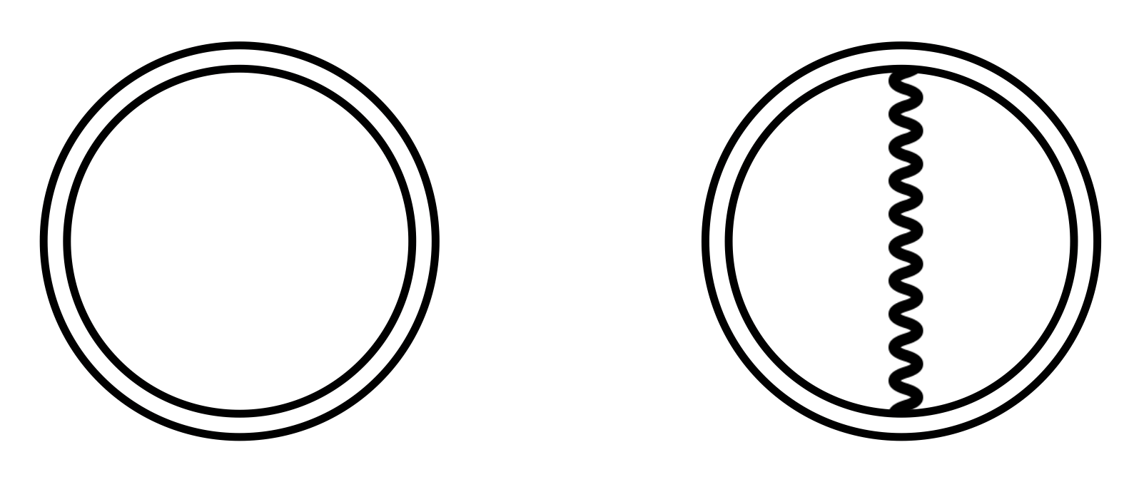
Figure 1: The irreducible one-loop (left) and two-loop (right) diagrams contributing to the Euler-Heisenberg effective Lagrangian, with the double solid lines representing the fully-dressed fermion propagator.

Thus, the full expansion (1) is a double series, an expansion both in $\alpha$ and in the field strength. We have separated a factor of $\left(\frac{\alpha}{\pi}\right)^{l}$ from our definition of ${\mathcal{L}}^{(l)}\!\left(\frac{eF}{m^{2}}\right)$, to emphasize the fact that the loop expansion (1) is a perturbative expansion, which is also expected to be asymptotic [32]. If the background field is magnetic, of magnitude $B$, at $l$-loop order ${\mathcal{L}}^{(l)}\!\left(\frac{eB}{m^{2}}\right)$ is expected to be unambiguously Borel summable to a real expression. If the background field is electric, of magnitude $E$, at $l$-loop order ${\mathcal{L}}^{(l)}\!\left(\frac{eE}{m^{2}}\right)$ is expected to have both real and imaginary parts, also expressible as a well-defined Borel representation. Furthermore, it is expected that at each loop order the electric background field result can be obtained by analytic continuation $B\to iE$ from the real magnetic field result. Here we analyze these issues beyond the familiar one-loop result, using ideas and methods from Borel-Écalle summation [33, 34, 35, 36, 37, 38, 39, 40].

At one-loop order the non-perturbative imaginary part has a well-known polylogarithm expression which can be expanded as a convergent weak-field instanton expansion:

$${\rm Im}\left[\mathcal{L}^{(1)}\left(\frac{eE}{m^{2}}\right)\right] = \frac{E^{2}}{2\pi}\,\text{Li}_{2}\quantity(e^{-\pi m^{2}/(eE)})$$ (3)

$$= \frac{E^{2}}{2\pi}\left\{e^{-\pi m^{2}/(eE)}+\frac{1}{2^{2}}e^{-2\pi m^{2}/(eE)}+\frac{1}{3^{2}}e^{-3\pi m^{2}/(eE)}+\ldots\right\}$$ (4)

Note that the instanton terms are not multiplied by fluctuation series, just numerical residue factors, so this is a very simple example of a trans-series. By contrast, at two-loop order the weak-field instanton expansion of the non-perturbative imaginary part is conjectured to be of the form [8, 9, 10, 11]

$${\rm Im}\left[{\mathcal{L}}^{(2)}\left(\frac{eE}{m^{2}}\right)\right]\sim\frac{\pi E^{2}}{2}\,\left\{e^{-\pi m^{2}/(eE)}\bigg{(}1+\dots\bigg{)}+\sqrt{\frac{m^{2}}{eE}}\sum_{k=2}^{\infty}e^{-k\pi m^{2}/(eE)}\left(-c_{k}+\sqrt{\frac{eE}{m^{2}}}+\ldots\right)\right\}$$ (5)

where the numerical coefficient $c_{k}$, for $k\geq 2$, is

$$c_{k}=\frac{1}{2\sqrt{k}}\sum_{\ell=1}^{k-1}\frac{1}{\sqrt{\ell(k-\ell)}}\qquad,\quad k\geq 2$$ (6)

This conjectured two-loop structure is quite different from one-loop: there are (unspecified) fluctuations about the one-instanton term, and at higher instanton orders ($k\geq 2$) there is a stronger weak-field prefactor, $\sqrt{\frac{m^{2}}{eE}}$, followed also by fluctuations (only partially specified). Our goal here is to investigate these fluctuation terms in the non-perturbative imaginary part for the two-loop effective Lagrangian in an electric background field, by analytic continuation from the weak field expansion for a magnetic background. We focus on reconstructing non-perturbative information from finite-order perturbative information, rather than the standard method of seeking an exact closed-form (multi-)integral representation, which currently appears prohibitively difficult even at three-loop order [17, 18, 19]. The motivation for this different approach is as a proof-of-principle test for a new approach to Euler-Heisenberg computations at higher loop order.

Note that while $eF$ is a renormalization group invariant, both $\alpha$ and $m^{2}$ are scale dependent. At one-loop order, $m^{2}$ is simply the bare mass and the charge renormalization is conventionally done at the physical electron mass scale. At two-loop order, a field-dependent mass renormalization is required, and ${\mathcal{L}}^{(2)}$ is again conventionally renormalized at the physical electron mass scale [8, 9, 10]. Being a doubly-perturbative expansion, it is not immediately obvious how to extract strong-field or short-distance or non-perturbative information from the full all-orders result (1). Different expansions, for example at fixed order in $\alpha$ or in $eF$, are possible, and correlated or uniform limits may also be physically relevant in certain circumstances. For example, if we sum the leading weak field contributions to the imaginary part of ${\mathcal{L}}^{(l)}\left(\frac{eE}{m^{2}}\right)$ for an electric background, this sum exponentiates to $e^{\alpha\pi}$ times the leading one-loop result [10, 41, 18]:

$${\rm Im}\left[\mathcal{L}\left(\alpha,\frac{eE}{m^{2}}\right)\right]\sim\frac{\alpha E^{2}}{2\pi^{2}}\,e^{\alpha\pi}\,e^{-\pi m^{2}/(eE)}+\dots\qquad,\quad eE\ll m^{2}$$ (7)

This exponential factor can be computed from the world-line representation of the effective Lagrangian [41], or can be understood [10] as encoding the leading field-dependent mass shift at two-loop order: $m^{2}\to m^{2}-\alpha/(eE)$. By a Borel dispersion relation, this exponentiation can be translated into a conjecture for the leading large-order growth of the perturbative expansion coefficients $a_{n}^{(l)}$ [15], which motivates the choice of overall normalization of these coefficients in (2).

Here we propose a different approach to the higher-loop computations, based on expressing the perturbative weak magnetic field expansion at a given loop order as an approximate Borel integral, whose strong-field limit can be extracted with surprisingly high precision, and whose analytic continuation from a magnetic to an electric background can also be achieved with high precision, including exponentially suppressed non-perturbative information. Such an approach relies on efficient and near-optimal methods to perform the necessary analytic continuations [38, 39, 40]. In this paper we test the feasibility of such methods applied to the Euler-Heisenberg effective Lagrangian at one-loop and two-loop, and we conclude with comments about the prospects for higher loop orders.

II The Exact One-loop Euler-Heisenberg Effective Lagrangian

II.1 Exact Results at One-Loop Order

We first review well-known properties of the one-loop Euler-Heisenberg QED effective Lagrangian in a constant background magnetic field, $B$, conventionally expressed as a proper-time integral [1, 5]

$$\mathcal{L}^{(1)}\left(\frac{eB}{m^{2}}\right)=-\frac{B^{2}}{2}\int_{0}^{\infty}\frac{\differential{t}}{t^{2}}\quantity(\coth t-\frac{1}{t}-\frac{t}{3})e^{-m^{2}t/(eB)}$$ (8)

[Recall our notational convention that a factor of $\left(\frac{\alpha}{\pi}\right)^{l}$ is extracted at $l$-loop order]. The weak field expansion of (8) is a prototypical effective field theory expansion, expressing the physics of the light fields (photons) after integrating out the heavy fields (electrons/positrons) at the electron mass scale $m$:

$$\mathcal{L}^{(1)}\left(\frac{eB}{m^{2}}\right)\sim\frac{B^{2}}{\pi^{2}}\quantity(\frac{eB}{m^{2}})^{2}\sum_{n=0}^{\infty}a_{n}^{(1)}\quantity(\frac{eB}{m^{2}})^{2n}\qquad,\quad eB\ll m^{2}$$ (9)

Here the factorially divergent one-loop expansion coefficients are known exactly:

$$a_{n}^{(1)} = (-1)^{n}\frac{\Gamma(2n+2)}{\pi^{2n+2}}\zeta(2n+4)$$ (10)

$$= (-1)^{n}\frac{\Gamma(2n+2)}{\pi^{2n+2}}\left(1+\frac{1}{2^{2}}\cdot\frac{1}{2^{2n+2}}+\frac{1}{3^{2}}\cdot\frac{1}{3^{2n+2}}+\frac{1}{4^{2}}\cdot\frac{1}{4^{2n+2}}+\dots\right)$$ (11)

The corrections to the leading factorial growth in (11) are exponential in $n$, which is directly related to the non-appearance of power-law fluctuation corrections in the instanton expansion (4) [5]. We have deliberately written the Riemann zeta factor in the form in (11) to emphasize the correspondence between the $\frac{1}{k^{2}}$ factors multiplying the $k$-instanton terms in (4), and the residues of the singularities of the Borel transform. See also Figure 7.

The exact integral representation (8) can also be expanded in the strong field limit, yielding a convergent strong field expansion whose leading behavior is:

$$\mathcal{L}^{(1)}\left(\frac{eB}{m^{2}}\right)\sim\frac{1}{3}\cdot\frac{B^{2}}{2}\quantity(\ln\left(\frac{eB}{\pi m^{2}}\right)-\gamma+\frac{6}{\pi^{2}}\zeta^{\prime}(2))\quad,\quad eB\gg m^{2}$$ (12)

where $\gamma\approx 0.5772...$ is the Euler-Mascheroni constant, and $\zeta^{\prime}(2)=\frac{1}{6}\pi^{2}(-12\log(A)+\gamma+\ln(2\pi))\approx-0.937548$, with $A$ being the Glaisher-Kinkelin constant. The coefficient $\frac{1}{3}$ of the logarithmic term in (12) is the one-loop QED beta function coefficient $\beta_{1}$, associated with one-loop charge renormalization [2, 5]:

$$\beta_{\rm QED}(\alpha)=2\alpha\sum_{n=1}^{\infty}\beta_{n}\left(\frac{\alpha}{\pi}\right)^{n}=2\alpha\quantity[\frac{1}{3}\left(\frac{\alpha}{\pi}\right)+\frac{1}{4}\left(\frac{\alpha}{\pi}\right)^{2}+\dots]$$ (13)

The weak field expansion (9) is an asymptotic series [3, 42, 43, 44, 45, 5], whose Borel sum is the one-loop Euler-Heisenberg integral representation (8), with one-loop Borel transform function:

$${\mathcal{B}}^{(1)}(t):=-\frac{1}{\pi^{2}\,t^{2}}\quantity(\coth(\pi t)-\frac{1}{\pi t}-\frac{\pi t}{3}) = \frac{2}{\pi^{3}}\sum_{n=0}^{\infty}(-1)^{n}\zeta(2n+4)\,t^{2n+1}$$ (14)

$$= \frac{2}{\pi^{3}}\sum_{k=1}^{\infty}\frac{t}{k^{2}(t^{2}+k^{2})}$$ (15)

Here we have chosen to make the convenient rescaling of the Borel variable by a factor of $\pi$, to absorb the powers of $1/\pi$ in (10)-(11), which has the effect of placing the Borel poles at integer multiples of $i$, rather than at integer multiples of $\pi i$. Then the exact one-loop effective Lagrangian is recovered via the Borel-Laplace integral (note the extra factor of $\pi$ in the exponent):

$$\mathcal{L}^{(1)}\left(\frac{eB}{m^{2}}\right)=\frac{\pi B^{2}}{2}\int_{0}^{\infty}dt\,e^{-m^{2}\pi t/(eB)}\,{\mathcal{B}}^{(1)}(t)$$ (16)

The small $t$ expansion (14) of ${\mathcal{B}}^{(1)}(t)$ generates the asymptotic weak magnetic field expansion (9), while the partial-fraction expansion in (15) exhibits the meromorphic nature of the one-loop Borel transform function ${\mathcal{B}}^{(1)}(t)$, with an infinite line of integer-spaced simple pole singularities along the imaginary Borel axis, at $t=\pm ik$, for $k=1,2,3,\dots$. Therefore, under analytic continuation, $B\to iE$, where $E$ is a constant background electric field, these poles lead to the non-perturbative imaginary part of the effective Lagrangian in (3), with weak-field expansion in (4). In the strong electric field limit the leading behavior can be obtained by analytic continuation from the strong magnetic field expansion in (12):

$${\rm Im}\left[\mathcal{L}^{(1)}\left(\frac{eE}{m^{2}}\right)\right]\sim\beta_{1}\left(\frac{\pi}{2}\right)\frac{E^{2}}{2}\quad,\quad eE\gg m^{2}$$ (17)

consistent with the strong field limit of the exact polylog expression in (3). This also follows from the explicit representation of the one-loop effective Lagrangian in terms of the Barnes gamma function $G$ [5]:

$$\mathcal{L}^{(1)}\quantity(\frac{eB}{m^{2}}) =\frac{2B^{2}}{m^{4}}\left[-\frac{1}{12}+\zeta^{\prime}(-1)+\frac{1}{16}\quantity(\frac{m^{2}}{eB})^{2}+\quantity(-\frac{1}{12}+\frac{m^{2}}{4eB}-\frac{1}{8}\quantity(\frac{m^{2}}{eB})^{2})\ln\frac{m^{2}}{2eB}\right.$$

$$\quad\Bigg{.}-\quantity(1-\frac{m^{2}}{2eB})\ln\Gamma\quantity(\frac{m^{2}}{2eB})-\ln G\quantity(\frac{m^{2}}{2eB})\Bigg{]}$$ (18)

This Barnes representation of the one-loop effective Lagrangian is particularly convenient for analytic continuation of $B$, since the analytic properties of the Barnes G function are well known [46, 47].

II.2 Borel Analysis at One-Loop Order

In preparation for the two-loop analysis, where a simple Borel representation of the form in (8) is not available, and a closed-form expression such as (18) in terms of a special function like the Barnes function is not known, we ask how we can recover accurate approximations to the various exact results listed in the previous sub-section. We do this here at one-loop and then extend these methods to two-loop order in Section III. Specifically, we begin with just a finite number of terms of the one-loop perturbative weak magnetic field expansion in (9), and seek to recover:

1. the strong magnetic field limit in (12) [this is a weak-field to strong-field extrapolation];

2. the non-perturbative imaginary part (4) of the effective Lagrangian in an electric field background [this is analogous to a Euclidean to Minkowski analytic continuation].

We develop a modified Padé-Borel approach that leads to remarkable precision with surprisingly little input information. Note that [48] has already showed that Padé-Borel summation achieves very accurate extrapolations of the weak magnetic field series for the one-loop Euler-Heisenberg effective Lagrangian. However, for the analysis at two-loop we require even higher precision; hence the new procedure described below.

Given only a finite number of terms of the weak magnetic field expansion (9), or equivalently only a finite number of terms in the small $t$ expansion of the Borel transform in (14)-(16), the key to an accurate extrapolation to other regions of the complex $B^{2}$ plane (recall that $B^{2}<0$ corresponds to an electric field background) is to have an accurate analytic continuation of the truncated Borel transform function

$$\mathcal{B}^{(1)}_{N}(t):=\frac{2}{\pi^{2}}\sum_{n=0}^{N-1}\frac{a_{n}^{(1)}}{(2n+1)!}\quantity(\pi t)^{2n+1}$$ (19)

Since the one-loop Borel transform is meromorphic, the optimal approach [39, 40] is to use a Padé approximation, which expresses $\mathcal{B}^{(1)}_{N}(t)$ as a ratio of polynomials:

$$\mathcal{P}_{[L,M]}\left({\mathcal{B}}^{(1)}_{N}(t)\right)=\frac{P^{(1)}_{L}(t)}{Q^{(1)}_{M}(t)}\quad,\quad\text{where}\quad\frac{P^{(1)}_{L}(t)}{Q^{(1)}_{M}(t)}=\mathcal{B}^{(1)}_{N}(t)+\mathcal{O}\left(t^{L+M+1}\right)$$ (20)

where $L+M=2N+1$. The zeros of the denominator polynomial $Q_{M}(t)$ approximate the true singularities (see (15)) of $\mathcal{B}^{(1)}(t)$, which lie at $t=\pm ik$ for $k\neq 0\in\mathbbm{Z}$ due to our rescaling $t\rightarrow\pi t$. See Figure 2. Tables of the one-loop Padé-Borel poles for $N=10$ input terms and for $N=50$ input terms are shown below in (21) and (22), in which we see poles stabilizing along the imaginary Borel axis at integer multiples of $\pm i$.

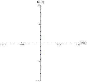
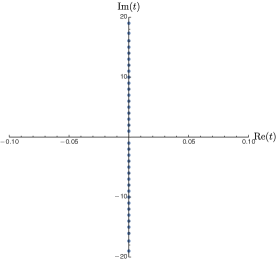
Figure 2: Poles of the Padé approximation $\mathcal{PB}_{N}^{(1)}(t)$ in (24) for the truncated Borel transform, shown for both $N=10$ (left) and $N=50$ (right). Note that all the poles lie on the imaginary axis and tend towards integer multiples of $\pm i$. This can be contrasted with two-loop case in Figure 8.

Padé poles from 10 input terms:

$$\pm\left\{1.0000i,2.0000i,3.0057i,4.2905i,8.0671i\right\}$$ (21)

Padé poles from 50 input terms:

$$\pm\left\{1.0000i,2.0000i,3.0000i,4.0000i,5.0000i,6.0000i,7.0000i,8.0000i,\right.$$

$$\left.\quad\ 9.0000i,10.000i,11.000i,12.000i,13.000i,14.000i,15.005i,16.062i,17.326i,\right.$$ (22)

$$\left.\quad\ 18.990i,21.239i,24.345i,28.798i,35.592i,47.048i,70.145i,139.79i\right\}$$

We dramatically improve the quality of the extrapolation if we take advantage of known information about the opposite (strong field) limit, which corresponds to including information about the $t\to\infty$ behavior of $\mathcal{B}^{(1)}(t)$. Here we appeal to the fundamental physical interpretation of the logarithmic behavior of the strong field expansion (12) in terms of charge renormalization and the conformal anomaly [1, 2, 8, 9, 5], which translates into the requirement that

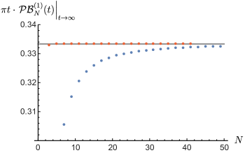
Figure 3: $N$ dependence of the limiting value $\lim\left[\pi t\cdot\mathcal{PB}_{N}^{(1)}(t)\right]_{t\to\infty}$, for $N$ ranging from 1 to 50, for the near-diagonal Padé approximant of the truncated one-loop Borel transform function in (24). The blue dots indicate the original values obtained from expanding $\pi t\cdot\mathcal{PB}_{N}^{(1)}(t)$ about $t\rightarrow\infty$, and which appear to be tending towards $1/3$. The red dots show a 4-th order Richardson extrapolation of this data. Observe that the physical value $\beta_{1}=1/3$ is approached quite closely already for $N\approx 10$.

$$\mathcal{B}^{(1)}(t)\sim\frac{\beta_{1}}{\pi t}+\dots\quad,\quad t\to+\infty$$ (23)

We therefore choose an off-diagonal Padé-Borel approximant with $M=L+1=N+1$

$$\mathcal{PB}^{(1)}_{N}(t):=\frac{P^{(1)}_{N}(t)}{Q^{(1)}_{N+1}(t)}$$ (24)

Note that we do not impose that the overall coefficient of $\pi t\cdot\mathcal{PB}^{(1)}_{N}(t)$ in the limit $t\to+\infty$ be equal to the physical value, $\beta_{1}=\frac{1}{3}$. We simply impose the functional form that $\pi t\cdot\mathcal{PB}^{(1)}_{N}(t)\to\text{constant}$, as $t\to+\infty$. Remarkably, the physical value, $\beta_{1}$, emerges in the large $N$ limit, already at $N\approx 10$. See Figure 3.

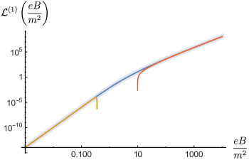
Figure 4: The blue curve is a log-log plot of the modified Padé-Borel sum of the truncated weak field expansion in (25), $\mathcal{L}_{N}^{(1)}$, plotted here using only $N=10$ perturbative input terms. This is indistinguishable from the exact closed-form Barnes function expression in (18), plotted here as the translucent blue band. The gold curve shows the weak field expansion (9), truncated at $N=10$. The red curve shows the leading strong field behavior of $\mathcal{L}^{(1)}$ in (12). Note that the truncated weak-field expansion fails even below the Schwinger limit $eB\approx m^{2}$, while the modified Padé-Borel sum accurately interpolates over many orders of magnitude between the weak-field and strong-field behavior. This plot was made using units in which $e=m^{2}=1$.

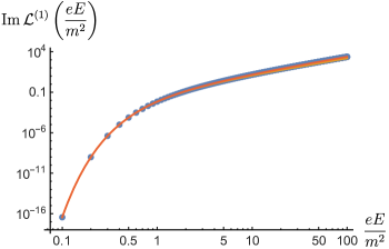
Figure 5: A log-log plot of the imaginary part of the electric field effective Lagrangian at one-loop, calculated using $N=10$ (blue dots). The gold curve shows the leading one-instanton contribution, $\propto\exp\quantity(-\pi m^{2}/(eE))$, which displays a small but noticeable deviation in the strong field limit. The red curve is the exact expression for the imaginary part in (3), including the sum over all instantons. See also Figure 6. This plot was made using units in which $e=m^{2}=1$.

With this procedure, our Padé analytic continuation (24) of the truncated weak-field expansion (19) leads to an approximate Borel-Laplace integral representation for the one-loop effective Lagrangian as in (16):

$$\mathcal{L}_{N}^{(1)}\left(\frac{eB}{m^{2}}\right)=\frac{\pi B^{2}}{2}\int_{0}^{\infty}\differential{t}\,e^{-m^{2}\pi t/(eB)}\,\mathcal{PB}^{(1)}_{N}\quantity(t)$$ (25)

Figure 4 shows the extrapolation of this expression from the weak-field limit to the strong-field limit. Starting with just ten input coefficients of the weak field expansion, the modified Padé-Borel expression in (25) extrapolates accurately over more than 8 orders of magnitude. This is a significantly farther-reaching extrapolation than in [48], due to our improved Padé-Borel transform in (24). This modified Padé-Borel transform also explains why the pole structure shown in Figure 2, and in Equations (21)-(22), is much more accurate than that in [48], where the physical form of the large $t$ behavior (23) was not imposed on the Padé-Borel transform.

Similarly we can use the approximate Borel representation in (25) to achieve our second goal: analytically continuing from a magnetic background to an electric background, to extract the exponentially small non-perturbative imaginary part of $\mathcal{L}^{(1)}$ in (3). Since the Borel singularities are all on the imaginary axis, we rotate the Borel contour to generate the imaginary part of the one-loop effective Lagrangian for a constant background electric field. Figure 5 shows (as blue dots) the result of this calculation, starting with 10 terms of the weak magnetic field expansion. The red curve shows the exact result in (3), summed over all instanton orders, while the gold curve shows the leading one-instanton term. The agreement is excellent in the weak-field limit, and also extrapolates accurately to much stronger fields.

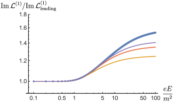
Figure 6: The ratio [blue dots] of the imaginary part of the electric field effective Lagrangian $\imaginary\mathcal{L}^{(1)}\quantity(E)$, divided by the leading exponential term from (4), derived from our extrapolation using as input just $N=10$ terms from the perturbative expression for a magnetic field background. The gold, red, and purple curves show a fit for this ratio, based on one, two, and three exponentially small correction terms, respectively. The fit coefficients are given in (26), from which it is clear that these sub-leading exponential corrections tend to the known form (3) of the instanton sum. This plot was made using units in which $e=m^{2}=1$.

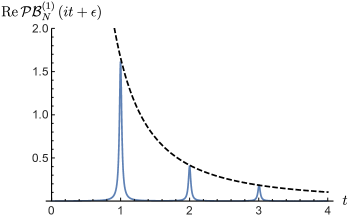
Figure 7: Singularity structure of the Borel transform $\mathcal{PB}_{N}^{(1)}(t)$, for $N=10$, just offset from the imaginary axis, $t\to it+\epsilon$. The plot shows the real part (blue solid curve) of $\mathcal{PB}_{N}^{(1)}(it+1/50)$, indicating integer-spaced poles at $t=ik$ along the imaginary Borel axis, with residues falling off quadratically as $1/k^{2}$ (dashed black curve).

In Figure 6 we show that the precision of our extrapolation is sufficiently high that we can probe the exponentially small higher-instanton corrections to $\imaginary\mathcal{L}^{(1)}\quantity(\frac{eE}{m^{2}})$, by dividing out the one-instanton factor, $E^{2}/(2\pi)\exp\quantity(-\pi m^{2}/(eE))$. Fitting this ratio with one-term, two-term and three-term exponential fits, we obtain the successively improving approximations:

$$\imaginary\mathcal{L}^{(1)}\left(\frac{eE}{m^{2}}\right)\approx\frac{E^{2}}{2\pi}\left(e^{-\pi m^{2}/(eE)}+0.253303\,e^{-2\pi m^{2}/(eE)}+\dots\right)$$

$$\imaginary\mathcal{L}^{(1)}\left(\frac{eE}{m^{2}}\right)\approx\frac{E^{2}}{2\pi}\left(e^{-\pi m^{2}/(eE)}+0.249962\,e^{-2\pi m^{2}/(eE)}+0.114532\,e^{-3\pi m^{2}/(eE)}+\dots\right)$$ (26)

$$\imaginary\mathcal{L}^{(1)}\left(\frac{eE}{m^{2}}\right)\approx\frac{E^{2}}{2\pi}\left(e^{-\pi m^{2}/(eE)}+0.249998\,e^{-2\pi m^{2}/(eE)}+0.111227\,e^{-3\pi m^{2}/(eE)}\right.$$

$$\hskip 113.81102pt\left.+0.0629846\,e^{-4\pi m^{2}/(eE)}+\dots\right)$$

We see that the coefficients of this instanton expansion approach the exact $\frac{1}{k^{2}}$ factors in (4). This demonstrates that our extrapolation from magnetic to electric field is exponentially accurate: it recovers several orders of the exponentially suppressed corrections to the non-perturbative imaginary part of the one-loop effective Lagrangian for an electric background field, using as input only 10 terms of the perturbative weak magnetic field expansion. Another way to see this is to plot our improved Padé-Borel transform (24), shifted slightly from the imaginary axis: Figure 7 shows the resulting poles at integer spacing along the imaginary axis, with residues following the exact $1/k^{2}$ behavior in (15).

III The Two-loop Euler-Heisenberg Effective Lagrangian

III.1 Exact Results at Two-Loop Order

Whereas the one-loop Euler-Heisenberg effective Lagrangian in a constant magnetic field has a simple Borel-Laplace integral representation (8), and can be expressed exactly in terms of the Barnes double gamma function (18), no such closed-form expressions are known at two-loop for a constant magnetic or electric field background. The most explicit representation for a magnetic background field is Ritus’s exact double-integral representation [8, 9, 10, 11]

$$\mathcal{L}^{(2)}\quantity(\frac{eB}{m^{2}})=\frac{B^{2}}{4}\int_{0}^{\infty}\frac{\differential{t}}{t^{3}}e^{-t\,m^{2}/(eB)}\quantity(J_{1}+J_{2}+J_{3})$$ (27)

where

$$J_{1} = \frac{2tm^{2}}{eB}\int_{0}^{1}\frac{\differential{s}}{s(1-s)}\quantity[\frac{\cosh(t\,s)\cosh(t(1-s))}{a-b}\ln\frac{a}{b}-t\coth t+\frac{5t^{2}}{6}s(1-s)]$$ (28)

$$J_{2} = -\int_{0}^{1}\frac{\differential{s}}{s(1-s)}\quantity[\frac{c}{(a-b)^{2}}\ln\frac{a}{b}-\frac{1-b\cosh(t(1-2s))}{b(a-b)}+\frac{b\cosh t+1}{2b^{2}}-\frac{5t^{2}}{6}s(1-s)]$$ (29)

$$J_{3} = \quantity(1+3\frac{tm^{2}}{eB}\quantity(\ln\left(\frac{tm^{2}}{eB}\right)+\gamma-\frac{5}{6}))\quantity(t\coth t-1-\frac{t^{2}}{3})$$ (30)

and the functions $a$, $b$ and $c$ are defined as

$$a=\frac{\sinh(t\,s)\sinh(t(1-s))}{t^{2}\,s(1-s)},\quad b=\frac{\sinh t}{t},\quad c=1-a\cosh(t(1-2s))$$ (31)

Unlike the one-loop case (8), this two-loop expression (27)-(31) is not directly in Borel form. However, we can expand this as a perturbative weak-field series in $\frac{eB}{m^{2}}$:

$$\mathcal{L}^{(2)}\quantity(\frac{eB}{m^{2}})\sim B^{2}\quantity(\frac{eB}{m^{2}})^{2}\sum_{n=0}^{\infty}a_{n}^{(2)}\quantity(\frac{eB}{m^{2}})^{2n}\quad,\quad eB\ll m^{2}$$ (32)

There is no simple closed-form expression for the coefficients $a_{n}^{(2)}$. However, the two-loop weak-field coefficients $a_{n}^{(2)}$ can be generated by a suitable expansion of the integral representation (27). In [14], 15 terms of such a weak magnetic field expansion were obtained, which was enough perturbative data to argue that the leading large order growth of the two-loop expansion coefficients $a_{n}^{(2)}$ has exactly the same form as the leading large order growth (11) of the one-loop expansion coefficients $a_{n}^{(1)}$:

$$a_{n}^{(2)} \sim (-1)^{n}\frac{\Gamma(2n+2)}{\pi^{2n+2}}+\text{corrections}\quad,\quad n\to\infty$$ (33)

In this paper we have pushed the perturbative expansion (32) to much higher order, obtaining 50 terms of the two-loop weak magnetic field expansion. This expansion must be organized appropriately to respect the various subtractions, in order to keep the $s$ integrals finite. Our expansion strategy is described in Appendix V. This new weak-field perturbative data confirms the leading result (33), and furthermore allows analysis of the subleading corrections: see Section III.2 below. The first 25 coefficients $a_{n}^{(2)}$ are listed in Appendix VI, and the first 50 coefficients are listed in an accompanying Supplementary file. This is the perturbative input data on which our subsequent Borel analyses are based.

The leading strong magnetic field behavior at two-loop order is also known [8, 9, 10]

$$\mathcal{L}^{(2)}\left(\frac{eB}{m^{2}}\right)\sim\frac{1}{4}\cdot\frac{B^{2}}{2}\quantity(\ln\left(\frac{eB}{\pi m^{2}}\right)-\gamma-\frac{5}{6}+4\zeta(3))\quad,\quad eB\gg m^{2}$$ (34)

where $\zeta(3)\approx 1.20206$. As in the one-loop case (12), we identify the two-loop QED beta function coefficient, $\beta_{2}=1/4$, in the prefactor of the leading logarithmic factor of the strong field limit (34).

Analytically continuing from a magnetic to an electric background, $B\to iE$, the results in (33) and (34) yield the leading contributions to the non-perturbative imaginary part of the two-loop effective Lagrangian $\mathcal{L}^{(2)}\left(\frac{eE}{m^{2}}\right)$:

$${\rm Im}\left[\mathcal{L}^{(2)}\left(\frac{eE}{m^{2}}\right)\right]\sim\begin{dcases}\frac{\pi E^{2}}{2}\,e^{-\pi m^{2}/(eE)}\quad,\quad eE\ll m^{2}\\ ~{}\\ \beta_{2}\quantity(\frac{\pi}{2})\frac{E^{2}}{2}\quad,\quad eE\gg m^{2}\end{dcases}$$ (35)

These leading behaviors at two-loop are structurally identical to the leading behaviors at one-loop order (recall (4) and (17)). However, we show below that the subleading corrections at two-loop order are very different from the corrections at one-loop order.

III.2 Borel Analysis at Two-Loop Order

Based on the leading factorial growth in (33), and in analogy to the one-loop case analyzed in Section II.2, we define the two-loop (truncated) Borel transform

$$\mathcal{B}^{(2)}_{N}(t):=2\sum_{n=0}^{N-1}\frac{a_{n}^{(2)}}{(2n+1)!}(\pi t)^{2n+1}$$ (36)

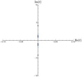
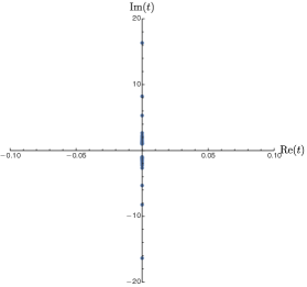
Figure 8: Poles of the Padé approximation $\mathcal{PB}^{(2)}_{N}(t)$ in (37) for the truncated Borel transform, shown for $N=10$ (left) and $N=50$ (right). Note that the poles appear to be accumulating at $\pm i$. Contrast with one-loop case in Figure 2 where the poles are integer-spaced along the imaginary Borel axis.

Note that we have adopted the same rescaling of $t$ by a factor of $\pi$, as at one loop in (19), because the leading growth of the two-loop coefficients in (33) matches that at one-loop (11). Recall also that at one-loop we obtained high-precision analytic continuations by using a modified Padé-Borel transform (24) that incorporated information about the strong magnetic field behavior of the one-loop effective Lagrangian. Since the strong magnetic field limit in (34) has the same functional form as at one-loop, (12), we adopt the same strategy here. We analytically continue the truncated Borel transform (36) via a near-diagonal Padé approximant, which encodes the logarithmic strong field behavior (34) at two-loop:

$$\mathcal{PB}^{(2)}_{N}(t)=\frac{P^{(2)}_{N}(t)}{Q^{(2)}_{N+1}(t)}$$ (37)

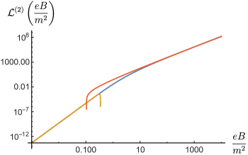
Figure 9: The blue curve is a log-log plot of the modified Padé-Borel sum of the truncated weak field expansion in (38), $\mathcal{L}^{(2)}_{N}$, plotted here for $N=10$. Compare with the one-loop result plotted in Figure 4. In contrast to the situation at one loop, there is no exact expression for the Lagrangian at two loop against which to compare the resummation. The gold curve shows the weak field expansion (32), truncated at $N=10$. The red curve shows the leading strong field behavior in (34). Once again, we see that the truncated weak field expansion fails before the Schwinger critical field $eB\approx m^{2}$, whereas the modified Padé-Borel sum interpolates over many orders of magnitude between the weak-field and strong-field behavior. This plot was made using units in which $e=m^{2}=1$.

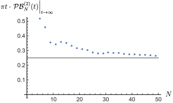
Figure 10: $N$ dependence of the limiting value $\lim\left[\pi t\cdot\mathcal{PB}_{N}^{(2)}(t)\right]_{t\to\infty}$, for $N$ ranging from 1 to 50, for the near-diagonal Padé approximant of the truncated one-loop Borel transform function in (37). The blue dots indicate the values obtained from expanding $\pi t\cdot\mathcal{PB}_{N}^{(1)}(t)$ about $t\rightarrow\infty$, and which tend towards the physical value $\beta_{2}=1/4$.

Figure 8 shows the singularities of this two-loop Padé-Borel transform, $\mathcal{PB}^{(2)}_{N}(t)$, based on 10 or 50 input coefficients (the first 25 coefficients are listed in Appendix VI, and the first 50 coefficients are listed in an accompanying Supplementary file). These plots confirm that the leading singularities are at $t=\pm i$, but they also show that the Borel plane singularity structure is much richer than in the one-loop case, where the singularities are just isolated poles at integer multiples of the leading ones: recall Figure 2. At two-loop, Figure 8 suggests that the leading singularities, at $t=\pm i$, appear to be branch points. Recall that a Padé approximant represents branch cuts as lines of poles (interlaced by the Padé zeros) that accumulate to the branch points [39, 40, 53]. This novel branch point structure is probed in more detail in Section III.3 below.

Given the Padé approximation (37) to the Borel transform, the approximate two-loop effective Lagrangian for the magnetic background is recovered by the Laplace transform

$$\mathcal{L}_{N}^{(2)}\!\left(\frac{eB}{m^{2}}\right)=\frac{\pi B^{2}}{2}\int_{0}^{\infty}\differential{t}\,e^{-m^{2}\pi t/(eB)}\,\mathcal{PB}^{(2)}_{N}\quantity(t)$$ (38)

The quality of this two-loop expression (38) as an accurate extrapolation of the two-loop effective Lagrangian $\mathcal{L}^{(2)}\!\left(\frac{eB}{m^{2}}\right)$ from weak magnetic field to strong magnetic field, and from magnetic to electric field, relies on the quality of the analytic continuation of the Borel transform in the Borel plane, here provided by the Padé approximation (37).

Using only 10 input perturbative coefficients $a_{n}^{(2)}$, in Figure 9 we plot the resulting Borel representation $\mathcal{L}_{N}^{(2)}\!\left(\frac{eB}{m^{2}}\right)$ from (38). Similar to the one-loop result in Figure 4, we see that our modified Padé-Borel representation at two-loop also extrapolates accurately over many orders of magnitude from the weak magnetic field to the strong magnetic field regime.

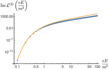
Figure 11: A log-log plot of the imaginary part (blue dots) of the two-loop effective Lagrangian in an electric field, calculated using $N=10$ input perturbative terms. The gold curve shows the leading weak-field one-instanton contribution in (35). This plot was made using units in which $e=m^{2}=1$.

The excellent agreement of this extrapolation to asymptotically large magnetic field can be attributed to the fact that we have constructed our Padé-Borel transform in such a way that it incorporates the form of the known logarithmic behavior (34) of the two-loop effective Lagrangian: the Borel transform, which is generated from an expansion about $t=0$, should be proportional to $1/(\pi t)$ as $t\to+\infty$. Note that, (as at one-loop) we do not enforce that the coefficient of proportionality be equal to $\beta_{2}$. Remarkably, once again this fact emerges from our 50 input coefficients, even though these coefficients were generated in the opposite limit near $t=0$. See Figure 10.

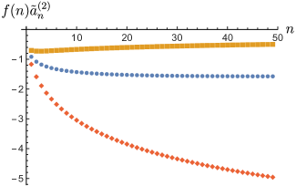
Figure 12: The large order behavior of the modified coefficients $\tilde{a}_{n}^{(2)}$ defined in (39). Different growth rates are shown here: $f(n)=(-1)^{n}\pi^{2n+2}/\Gamma\quantity(2n+\frac{5}{4})$ (blue circles), $f(n)=(-1)^{n}\pi^{2n+2}/\Gamma\quantity(2n+\frac{5}{4}+\frac{1}{4})$ (gold squares), and $f(n)=(-1)^{n}\pi^{2n+2}/\Gamma\quantity(2n+\frac{5}{4}-\frac{1}{4})$ (red diamonds). The form involving $\Gamma(2n+\frac{5}{4})$ is clearly favored.

We can also use the approximate Borel expression (38) to achieve our second goal: analytic continuation from a magnetic to an electric background, producing an exponentially small non-perturbative imaginary part of $\mathcal{L}_{N}^{(2)}\!\left(\frac{eE}{m^{2}}\right)$. The result is shown in Figure 11, again showing good agreement over many orders of magnitude of the external field strength. However, there is a clear deviation from this leading weak field contribution even at $eE\approx m^{2}$, coming from fluctuations about this one instanton term which were not present at one-loop in (4). This deviation is analyzed in the next Section. See Figure 13.

III.3 Power Law Corrections at Two-Loop Order

The Padé-Borel pole structure in Figure 8 suggests that the leading singularities at two-loop are branch points rather than poles. However, the leading large-order growth in (33) is the same as the one-loop leading large-order growth in (10), and this leading growth is associated with Borel poles. The resolution of this apparent puzzle is that each of the symmetric leading Borel singularities, at $t=\pm i$, is in fact a superposition of a pole and a branch point. This cannot be seen directly from the Padé poles in Figure 8. To resolve this Borel singularity structure, we subtract the exact leading growth behavior and study the remainder, defining modified perturbative weak-field expansion coefficients

$${\tilde{a}}^{(2)}_{n}\equiv a^{(2)}_{n}-(-1)^{n}\frac{\Gamma(2n+2)}{\pi^{2n+2}}$$ (39)

We now analyze the large order behavior of the modified coefficients ${\tilde{a}}^{(2)}_{n}$. Ratio tests indicate the following leading growth of the ${\tilde{a}}^{(2)}_{n}$:

$${\tilde{a}}^{(2)}_{n}\approx\quantity(-1.65)\times(-1)^{n}\frac{\Gamma\left(2n+\frac{5}{4}\right)}{\pi^{2n+2}}+\dots$$ (40)

See Figure 12, where we have adjusted the offset shift, finding the best agreement with the offset $\frac{5}{4}$.

After analytic continuation to an electric field, this corresponds to the following power-law correction to the imaginary part of the two-loop effective Lagrangian:

$${\rm Im}\left[{\mathcal{L}}^{(2)}\left(\frac{eE}{m^{2}}\right)\right]\sim\frac{\pi E^{2}}{2}\,e^{-\pi m^{2}/(eE)}\bigg{[}1-1.65\left(\frac{eE}{\pi m^{2}}\right)^{3/4}+\dots\bigg{]}$$ (41)

This form of the leading correction suggests a fluctuation expansion in powers of $\left(\frac{eE}{m^{2}}\right)^{3/4}$:

$${\rm Im}\left[{\mathcal{L}}^{(2)}\left(\frac{eE}{m^{2}}\right)\right]\sim\frac{\pi E^{2}}{2}\,e^{-\pi m^{2}/(eE)}\bigg{[}1+d_{1}\left(\frac{eE}{\pi m^{2}}\right)^{3/4}+d_{2}\left(\frac{eE}{\pi m^{2}}\right)^{3/2}+d_{3}\left(\frac{eE}{\pi m^{2}}\right)^{9/4}+\dots\bigg{]}$$ (42)

In Figure 13 we plot the result of fitting the imaginary part of the two-loop effective Lagrangian directly from the integral representation. Using the fit interval $\frac{eE}{m^{2}}\in[10^{-1},1]$ we obtain fit parameters: $d_{1}=-1.65$, $d_{2}=2.43$, $d_{3}=-1.94$. Figure 13 illustrates the improved agreement with the successive weak-field corrections. This form of the fluctuations about the one-instanton term fills in the first set of missing dots in Ritus’s conjectured expression (5).

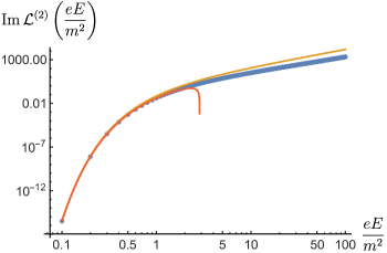
Figure 13: The imaginary part of the electric field effective Lagrangian (blue dots), compared with the leading weak-field one-instanton contribution (gold), and the fit including the additional weak-field power-law corrections in (42) (red). This plot was made using units in which $e=m^{2}=1$.

III.4 Probing the Higher Instanton Terms

In fact, the power-law corrections discussed in the previous Section are not the whole story. The weak-field expressions in (35) and (42) only include the effects of the leading Borel singularity at $t=\pm i$: these are the “one-instanton” effects. But we also expect that there should be multi-instanton effects associated with Borel singularities at all integer multiples of the leading ones. These would appear as exponentially small corrections to the large-order growth of the perturbative expansion coefficients $a_{n}^{(2)}$. Therefore, the subleading corrections to the large order growth of the two-loop perturbative expansion coefficients should have the following structural form:

$$a_{n}^{(2)} \sim (-1)^{n}\frac{\Gamma(2n+2)}{\pi^{2n+2}}\left\{\big{(}\text{1+power law corrections}\big{)}\right.$$ (43)

$$\left.\qquad\qquad+\big{(}\text{exponentially small corrections}\big{)}\times\big{(}\text{power law corrections}\big{)}\right\}$$

Even though the leading large-order growth has the same form as at one-loop, compare (11) and (33), the structure of the corrections is very different: there are power-law corrections followed by much smaller exponentially suppressed corrections, which themselves have power-law corrections. This fact is directly responsible for the novel structure (5) of the non-perturbative imaginary part at two-loop order. Having studied the structure of the power-law corrections in the previous subsection, we now turn to the exponentially smaller corrections.

At one-loop the first few exponentially small corrections can be resolved, see Figure 6, because there are no power-law corrections (recall (11)), but at two-loop it is much more difficult because of the existence of the (much larger) power-law corrections to the leading instanton term. These power-law corrections obscure the exponentially small corrections associated with multi-instantons. This problem can be ameliorated by using more sophisticated Borel techniques, beyond Padé-Borel. Indeed, this problem is directly related to the fact that the Padé-Borel approximation represents the leading branch cut as a line of poles, which therefore obscures the existence of genuine multi-instanton singularities, which also lie on the imaginary axis, and are also expected to be branch points. See Figure 14, which plots the Padé-Borel transform along the imaginary axis: the leading singularity at $t=i$ can be seen, but beyond that one sees coalescing Padé poles that are attempting to represent the branch cut $t\in[i,i\,\infty]$. This also explains why the multi-instanton Borel singularities are clear at one-loop from the Padé-Borel pole distribution in Figure 2 (because they are simple poles), but are not seen directly at two-loop order from the Padé-Borel pole distribution in Figure 8 (because they are branch points). Fortunately, there is a simple way to resolve this problem.

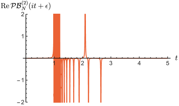
Figure 14: Plot of the real part of the Padé-Borel transform, $\real[\mathcal{PB}_{N}^{(2)}(it+1/1000)]$ for $N=50$, showing the singularity structure of the Padé-Borel transform along the imaginary axis. Note that without the conformal map, the accumulation of poles from the Padé-Borel approximation obscures the true singularity structure associated with the physical higher instanton terms. Compare with Figure 16 where the physical multi-instanton Borel singularities at $t=2i$ and $t=3i$ are resolved.

The first step is to confirm that there are indeed integer-repeated Borel singularities, and to determine if they are in fact branch points. This problem can be resolved as follows [38, 39, 40]. We use a conformal map [49, 54, 55] to map the doubly-cut Borel plane (based on the two symmetric leading branch point singularities at $t=\pm i$) into the unit disk in the conformal $z$ plane. Specifically, the relevant conformal map for this configuration is:

$$t=\frac{2z}{1-z^{2}}\qquad,\qquad z=\frac{t}{1+\sqrt{1+t^{2}}}$$ (44)

A re-expansion inside the unit disk to the original order, followed by a Padé approximation within the unit disk, separates subleading branch-points [38, 39, 40], as shown in Figure 15.

The doubly-cut $t$ plane is mapped to the interior of the unit disk, with the edges of the cuts mapped to segments of the boundary, the unit circle. We expand the truncated Borel transform inside the conformal disk, and truncate at the same order as the $t$ expansion:

$${\mathcal{B}}_{N}^{(2)}\left(\frac{2z}{1-z^{2}}\right)=\sum_{n=0}^{2N-1}b_{n}^{(2)}\,z^{n}+\mathcal{O}(z^{2N})$$ (45)

This expansion uniquely defines the coefficients $b_{n}^{(2)}$. By construction, this expansion is convergent within the conformal disk. We then make a near-diagonal Padé approximation, and compute its poles. These singularities are shown in Figure 15.

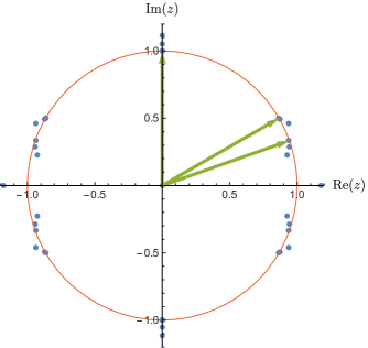
Figure 15: Poles of the Padé-Borel approximation in the conformally mapped $z$ plane. With $N=50$ terms, the first three Borel singularities can be resolved as accumulation points of Padé poles located on the unit circle at $\theta=\pm\frac{\pi}{2},\pm\frac{\pi}{6},\pm\arctan\quantity(\frac{1}{2\sqrt{2}})$, denoted by the green arrows.

The poles accumulating to $z=\pm i$ correspond to the leading singularities, since the conformal map (44) takes $t=\pm i$ to $z=\pm i$. The next cluster of poles accumulate to $z=\pm e^{\pm i\pi/6}$, which are the conformal map images (on either side of the leading branch cuts) of the two-instanton singularities at $t=\pm 2i$. The third cluster of $z$-plane poles in Figure 15 accumulate to the images of the three-instanton singularities at $t=\pm 3i$. Thus the conformal map reveals the existence of integer-repeated higher instanton Borel singularities, and shows that they all have associated branch cuts.

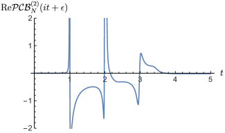
Figure 16: Plot of the real part of the Padé-Conformal-Borel transform, $\real[\mathcal{PCB}_{N}^{(2)}(it+1/1000)]$ for $N=50$, showing the singularity structure of the conformally mapped Borel transform along the imaginary axis. The plot reveals the existence of higher Borel singularities at multiples of the leading singularity at $t=i$, corresponding to the multi-instanton expansion. It also confirms the branch cut nature of the singularity structure at two loop. Compare with Figure 7 at one loop, where the Borel singularities are simple poles, and compare with the analogous plot at two loop, but without the conformal map, in Figure 14.

This resolution phenomenon can also be visualized by mapping the Padé approximation within the $z$-plane disk back to the Borel $t$ using the inverse transformation in (44) [38, 40]. This produces the Padé-Conformal-Borel approximation, and this is plotted along the imaginary $t$ axis in Figure 16. We see that the one-instanton, two-instanton and three-instanton singularities are all resolved. This should be contrasted with the result of the Padé-Borel approximation, without the conformal map, where nothing beyond the one-instanton singularity can be clearly resolved: recall Figure 14. This failure of the Padé-Borel approximation to resolve higher instanton singularities is a direct consequence of the fact that the Padé approximation represents the leading branch cuts as sequences of poles accumulating to the leading branch points, as seen in Figure 14, and these poles obscure the existence of the genuine physical higher-instanton singularities, which are themselves branch points. The conformal mapping resolves this problem, as can be seen in Figure 16.

To find the nature of the two-instanton Borel singularity at $t=\pm 2i$, we study the approach to the point $z=e^{i\pi/6}$ in the conformal disk. Writing $z=r\,e^{i\pi/6}$, we assume a power-law behavior $(1-r)^{\beta}$ for the imaginary part of the Borel transform, and fit a good fit with $\beta=-\frac{3}{2}$. See Figure 17. When mapped back to the Borel $t$ plane, this corresponds to an imaginary part of the two-loop effective Lagrangian, at the two-instanton level, of the form

$${\rm Im}\left[{\mathcal{L}}^{(2)}\left(\frac{eE}{m^{2}}\right)\right]_{\text{two-instanton}}\sim\frac{\pi E^{2}}{2}\,\sqrt{\frac{m^{2}}{eE}}\,e^{-2\pi m^{2}/(eE)}$$ (46)

which agrees with the form of the higher-instanton fluctuation prefactor conjectured by Ritus: recall Eq. (5). It is quite remarkable that this doubly-exponentially-suppressed term can be deduced directly from just the first 50 perturbative expansion coefficients of the effective Lagrangian in a magnetic field background.

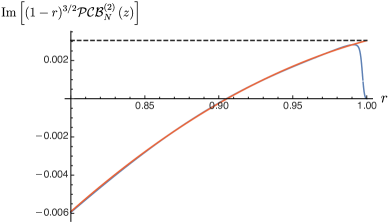
Figure 17: Blue: plot of the imaginary part of $(1-r)^{3/2}$ times the Padé-Conformal-Borel transform along the radial line $z=r\,e^{i\pi/6}$ inside the conformal disk, approaching the $z$-plane image of the two-instanton Borel singularity. Red: approximate extrapolation of this plot to the singularity at $z=e^{i\pi/6}$.

IV Conclusions

We have shown that accurate extrapolations and analytic continuations of the two-loop Euler Heisenberg effective Lagrangian can be recovered from a relatively modest number of terms of the perturbative weak magnetic field expansion. These perturbative terms are generated from an expansion of Ritus’s seminal results for the renormalized two-loop effective Lagrangian in terms of two-parameter integrals [8, 9, 10, 11]. The new physical effect at two-loop, compared to the well-known one-loop Euler-Heisenberg effective Lagrangian, is that the Borel transform has branch point singularities, rather than just simple poles. These branch points reflect the interactions between virtual particles, and have the effect of producing fluctuation expansions multiplying the terms in the weak-field instanton expansion for the imaginary part of the effective Lagrangian in an electric field background. In order to probe these fluctuation corrections we need high precision extrapolations, which we achieve using a combination of Padé approximations and conformal maps to obtain a sufficiently accurate analytic continuation of the finite order truncation of the associated Borel transform [39, 40]. We have also incorporated the known physical information about the strong magnetic field limit, which is fixed by the QED beta function, and which determines the functional form of the asymptotic limit of the Borel transform. In particular, with the input of just 10 terms of the perturbative weak field expansion we find an accurate extrapolation from the weak magnetic field regime to the strong magnetic field regime, over many orders of magnitude. See Figures 4 and 9 for the one-loop and two-loop results, respectively. Using 50 terms of the perturbative weak magnetic field expansion at two-loop order, we analytically continue to an electric field background and obtain new information about the structure of the instanton expansion of the imaginary part of the effective Lagrangian. We resolve the leading power law correction at the one-instanton level, and also identify the exponentially further suppressed two-instanton term.

Our analysis was motivated by the question of whether such extrapolations and associated non-perturbative information could be accessible at higher loop order (i.e. higher terms in the expansion (1) in the fine structure constant), starting not from a closed form multi-parameter integral representation, but from an explicit finite order perturbative expansion. This is because even at three-loop order (see Figure 18) it has so far not been possible to find a parametric integral representation (a $4$-fold parameter integral at three loop) of the Euler Heisenberg effective Lagrangian, even though the exact propagators in a constant background field are known in a relatively simple integral representation form [17, 18, 19]. Our results suggest that an alternative strategy might be more practical: work instead with a perturbative expansion of the propagators, thereby generating a finite-order perturbative expansion of the $l$-loop effective Lagrangian, from which extrapolations to other parametric regimes could be performed. To be practical, such extrapolations must be achievable with a “reasonable” amount of perturbative input, and our results suggest that this may indeed be possible. To generate the perturbative expansion at higher loop order, one needs an efficient way to compute the renormalized effective Lagrangian, for example using the background-field integration-by-parts methods developed in [16, 56].

Certain structural facts are known about the Euler Heisenberg effective Lagrangian at higher loop orders, and these could be used to constrain the higher-loop computations. The exponentiation $e^{\alpha\pi}$ of the leading weak electric corrections to the imaginary part, as in (7), leads to a conjecture [15] that the leading large order behavior of the perturbative expansion coefficients has the same form for all loop orders $l$:

$$a_{n}^{(l)} \sim (-1)^{n}\frac{\Gamma(2n+2)}{\pi^{2n+2}}\qquad,\quad n\to\infty\quad,\quad\forall\,l$$ (47)

Indeed, this conjectured behavior is the reason for the choice of the overall normalization of the perturbative expansion coefficients in (2): with this normalization choice we recover the exponential factor $e^{\alpha\pi}$ in (7). This conjecture, along with the exponentiation in (7), would be interesting to confirm or disprove beyond two-loop order. Physically, this correspondence is motivated by the interpretation of the mass $m$ appearing in the exponential instanton factor, $e^{-\pi m^{2}/(eE)}$, as the renormalized physical electron mass [10]. Already at two-loop order, this correspondence between the renormalized mass defined from the real or imaginary part of the effective Lagrangian is sensitive to the finite mass renormalization. The situation at three-loop order is not yet clear [17, 18, 19], and we hope that the methods described here might provide an alternative approach to shed light on this open question.

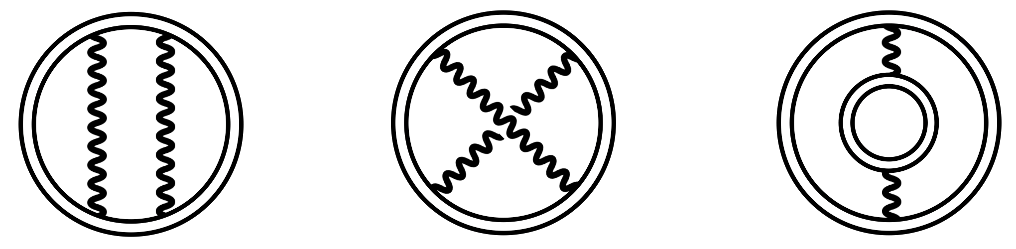
Figure 18: The three diagrams which contribute to the Euler-Heisenberg effective Lagrangian at $l=3$ loop order.

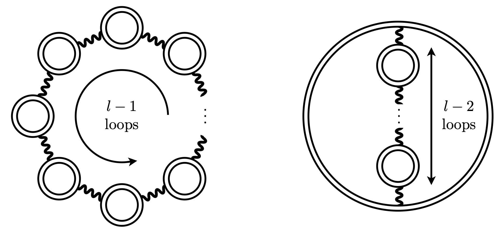
Figure 19: Two equivalent views of the irreducible $l$-loop diagram giving the dominant strong-field behavior in (48) for the $l$-loop Euler-Heisenberg effective Lagrangian. There are $(l-1)$ fermion loops, with the double lines denoting fermion propagators in the constant background field, and one overall photon loop.

The leading strong magnetic field behavior at $l$-loop order (with $l\geq 2$) is also known, arising from the Callan-Symanzik equation in the strong field (or massless) limit [8, 9, 10]:

$$\mathcal{L}^{(l)}\left(\frac{eB}{m^{2}}\right)\propto\frac{B^{2}}{2}\left(\ln\left(\frac{eB}{\pi m^{2}}\right)\right)^{l-1}+\dots\quad,\quad eB\gg m^{2}$$ (48)

The overall coefficient is expressed in terms of the beta function coefficients up to order $l$. This leading contribution comes from the renormalon-like “ring diagram” with $(l-1)$ fermion loops connected in a single ring by $(l-1)$ photon propagators. See Figure 19. This general fact could be used to constrain the asymptotic behavior of the Borel transform at $l$-loop order. Deeper understanding of the strong field limit at higher order in the fine structure constant $\alpha$ may also shed light on the computation of scattering amplitudes in strong background fields, in particular those associated with ultra-intense lasers [23, 24]. For example, seminal work by Ritus and Narozhnyi has made predictions for the resulting structure at higher loop order for the special case where the background laser field is represented as a constant crossed field [25, 26, 27, 28, 29, 30, 31].

V Appendix: Ritus’s Exact Double-Integral Representation

The two-loop Euler-Heisenberg effective Lagrangian can be written as the double integral

$$\mathcal{L}^{(2)}\quantity(\frac{eB}{m^{2}}) =\frac{B^{2}}{4}\int_{0}^{\infty}\frac{\differential{t}}{t^{3}}e^{-tm^{2}/(eB)}\quantity(J_{1}+J_{2}+J_{3})$$ (49)

with

$$J_{1} = \frac{2tm^{2}}{eB}\int_{0}^{1}\frac{\differential{s}}{s(1-s)}\quantity[\frac{\cosh ts\cosh t(1-s)}{a-b}\ln\frac{a}{b}-t\coth t+\frac{5t^{2}}{6}s(1-s)]$$ (50)

$$J_{2} = -\int_{0}^{1}\frac{\differential{s}}{s(1-s)}\quantity[\frac{c}{(a-b)^{2}}\ln\frac{a}{b}-\frac{1-b\cosh t(1-2s)}{b(a-b)}+\frac{b\cosh t+1}{2b^{2}}-\frac{5t^{2}}{6}s(1-s)]$$ (51)

$$J_{3} = \quantity(1+3\frac{tm^{2}}{eB}\quantity(\ln\left(\frac{tm^{2}}{eB}\right)+\gamma-\frac{5}{6}))\quantity(t\coth t-1-\frac{t^{2}}{3})$$ (52)

and

$$a=\frac{\sinh ts\sinh t(1-s)}{t^{2}s(1-s)},\quad b=\frac{\sinh t}{t},\quad c=1-a\cosh t(1-2s)$$ (53)

To generate a weak magnetic field expansion, for $J_{1}$ and $J_{2}$ we expand each term in the above expressions at small $t$ to order $\mathcal{O}(t^{2n})$. This is straightforward for most terms, with

$$\ln\frac{a}{b}=\sum_{k=0}^{n}\frac{2^{2k}\quantity(s^{2k}+(1-s)^{2k}-1)}{2k(2k)!}t^{2k}$$ (54)

For the factors $\quantity(a-b)^{-p}$, we first expand

$$a-b=t^{2}\sum_{k=0}^{n-1}\quantity[\frac{1}{(2k+4)!}\frac{1-(1-2s)^{2k+4}}{2s(1-s)}-\frac{1}{(2k+3)!}]t^{2k}=t^{2}\sum_{k=0}^{n-1}A_{k}t^{2k}$$ (55)

Then, the coefficients of this Taylor series raised to an arbitrary negative power can be generated recursively

$$(a-b)^{-p}=\frac{1}{t^{2p}}\sum_{k=0}^{n+p}A^{(-p)}_{k}t^{2k}$$ (56)

where (for $A_{0}\neq 0$)

$$A_{0}^{(-p)} =\frac{1}{A_{0}^{p}}$$ (57)

$$A_{k}^{(-p)} =\frac{1}{kA_{0}}\sum_{\ell=1}^{k}\quantity[\ell(1-p)-k]A_{\ell}A^{(-p)}_{k-\ell},\quad k\geq 1$$ (58)

We then combine these expansions using a discrete convolution

$$\quantity(\sum_{k=0}^{n}a_{k}t^{2k})\quantity(\sum_{k=0}^{n}b_{k}t^{2k})=\sum_{k=0}^{n}c_{k}t^{2k}$$ (59)

$$c_{k}=\sum_{\ell=0}^{k}a_{\ell}b_{k-\ell}$$ (60)

Although certain terms in $J_{1}$ and $J_{2}$ look divergent with respect to the $s$ integral, they are exactly canceled by the expansion of other terms in the integrand. In addition, each of the remaining terms contains a factor of $s(1-s)$, leaving well-defined integrals which result in polynomials in $t$. For $J_{3}$, there is no $s$ integral to perform, and so we can just expand the entire expression at small $t$ to $\mathcal{O}(t^{2n})$, yielding polynomials in $t$ and polynomials multiplied by $\ln\frac{tm^{2}}{eB}$. Now, all the $t$ integrals can be performed, where we can make use of the result

$$\int_{0}^{\infty}\differential{t}e^{-m^{2}t/(eB)}t^{2n}\ln\left(\frac{tm^{2}}{eB}\right)=\quantity(\frac{eB}{m^{2}})^{2n+1}\Gamma(2n+1)\psi^{(0)}(2n+1),\quad n>-\frac{1}{2}$$ (61)

with $\psi^{(0)}(x)$ the digamma function. With this algorithm, we were able to generate fifty coefficients in the weak magnetic field expansion of $\mathcal{L}^{(2)}\quantity(\frac{eB}{m^{2}})$, whereas previous analysis only obtained fifteen coefficients [14]. The first 25 weak magnetic field expansion coefficients of the two loop Euler-Heisenberg Lagrangian can be found in Appendix VI, and the first 50 coefficients are contained in an accompanying Supplementary file.

VI Appendix: Coefficients of the Two-Loop Weak Magnetic Field Expansion

$n$	$a_{n}^{(2)}$
$0$	$\displaystyle\frac{4}{81}$
$1$	$\displaystyle-\frac{1219}{32400}$
$2$	$\displaystyle\frac{33827}{396900}$
$3$	$\displaystyle-\frac{98923}{255150}$
$4$	$\displaystyle\frac{532455472}{180093375}$
$5$	$\displaystyle-\frac{10457103346}{307432125}$
$6$	$\displaystyle\frac{8280132424}{15035625}$
$7$	$\displaystyle-\frac{1322128891875104}{110718132525}$
$8$	$\displaystyle\frac{216079874926085406464}{646561329789375}$
$9$	$\displaystyle-\frac{399159024629278987264}{34029543673125}$
$10$	$\displaystyle\frac{118088344460059990083104768}{234021171840080625}$
$11$	$\displaystyle-\frac{10979187935861311150383104}{420447667696875}$
$12$	$\displaystyle\frac{18653011055800029685394341888}{11654809348557375}$
$13$	$\displaystyle-\frac{1635567621127339081554728370176}{14265121494999375}$
$14$	$\displaystyle\frac{214273566180161138094998308030185472}{22571190592506430875}$
$15$	$\displaystyle-\frac{25109740072479538970451463102102765568}{27910612022991823125}$
$16$	$\displaystyle\frac{764034086290611781552561173252582378831872}{7896673339814104720875}$
$17$	$\displaystyle-\frac{5323656802968440248000341338657607172260626432}{454224613538046611885625}$
$18$	$\displaystyle\frac{214511358602073886111889879319593742860030050304}{135039749970770614344375}$
$20$	$\displaystyle\frac{266462893626229350602869353007174008140288948032879198208}{6672849284578939554478010625}$
$21$	$\displaystyle-\frac{2437894565001775347497238208128324910365652981172597161984}{332534017503933864841096875}$
$22$	$\displaystyle\frac{102630737774414418996011603373560456263255744267423025320689664}{69566951104903323342538824375}$
$23$	$\displaystyle-\frac{264983617781753579377541150234960277977765158821145927518255054848}{817620826815723148073039559375}$
$24$	$\displaystyle\frac{34888103723767870212111639769661161527345864219016664926050448310272}{450525761714786224448409553125}$

- [1] W. Heisenberg and H. Euler, “Folgerungen aus der Diracschen Theorie des Positrons”, Z. Phys. 98, 714 (1936).
- [2] V. Weisskopf, “Über die Elektrodynamik des Vakuums auf Grund der Quantentheorie des Elektrons”, Kong. Dans. Vid. Selsk. Math-fys. Medd. XIV No. 6 (1936), reprinted in Quantum Electrodynamics, J. Schwinger (Ed.) (Dover, New York, 1958).
- [3] J. Schwinger, “On Gauge Invariance and Vacuum Polarization”, Phys. Rev. 82, 664 (1951).
- [4] W. Dittrich and M. Reuter, Effective Lagrangians in Quantum Electrodynamics, (Springer, 1985).
- [5] G. V. Dunne, “Heisenberg-Euler Effective Lagrangians: Basics and Extensions”, in Ian Kogan Memorial Collection, From Fields to Strings: Circumnavigating Theoretical Physics, Vol. I, M.A. Shifman et al. (Eds.), World Scientific, Singapore, 2004, 445 [hep-th/0406216].
- [6] V. Fock, “Proper Time In Classical And Quantum Mechanics,” Phys. Z. Sowjetunion 12, 404 (1937).
- [7] Y. Nambu, “The Use Of The Proper Time In Quantum Electrodynamics,” Prog. Theor. Phys. 5, 82 (1950).
- [8] V. I. Ritus, “Lagrangian of an intense electromagnetic field and quantum electrodynamics at short distances”, Zh. Eksp. Teor. Fiz. 69 (1975) 1517 [Sov. Phys. JETP 42, 774 (1976).
- [9] V. I. Ritus, “Connection between strong-field quantum elctrodynamics with short-distance quantum electrodyanmics”, Zh. Eksp. Teor. Fiz. 73 (1977) 807 [Sov. Phys. JETP 46, 423 (1977)].
- [10] V. I. Ritus, “Effective Lagrange Function of Intense Electromagnetic Field in QED”, in Proc. of Frontier Tests of Quantum Electrodynamics and Physics of the Vacuum, Sandansky 1998, (Heron Press, 1998), [arXiv:hep-th/9812124].
- [11] S.L. Lebedev and V.I. Ritus, “Virial representation of the imaginary part of the Lagrange function of the electromagnetic field”, Zh. Eksp. Teor. Fiz. 86 (1984) 408, [Sov. Phys. JETP 59 (1984) 237].
- [12] D. Fliegner, M. Reuter, M. G. Schmidt and C. Schubert, “Two-loop Euler-Heisenberg Lagrangian in dimensional regularization,” Theor. Math. Phys. 113, 1442 (1997) [Teor. Mat. Fiz. 113, 289 (1997)] [arXiv:hep-th/9704194].
- [13] B. Kors and M. G. Schmidt, “The effective two-loop Euler-Heisenberg action for scalar and spinor QED in a general constant background field,” Eur. Phys. J. C 6, 175 (1999) [arXiv:hep-th/9803144].
- [14] G. V. Dunne and C. Schubert, “Two loop Euler-Heisenberg QED pair production rate,” Nucl. Phys. B 564, 591-604 (2000), arXiv:hep-th/9907190.
- [15] G. V. Dunne and C. Schubert, “Multiloop information from the QED effective Lagrangian,” J. Phys. Conf. Ser. 37, 59-72 (2006), arXiv:hep-th/0409021.
- [16] M. Krasnansky, PhD Dissertation, University of Connecticut, 2007.
- [17] I. Huet, D. G. C. McKeon and C. Schubert, ‘Three-loop Euler-Heisenberg Lagrangian and asymptotic analysis in 1+1 QED,” pg 505-512, in Quantum Field Theory Under the Influence of External Conditions (QFEXT09), K. A. Milton and M. Bordag (Eds.), (World Scientific, Singapore, 2010), arXiv:0911.0227.
- [18] I. Huet, M. Rausch de Traubenberg and C. Schubert, “Asymptotic Behaviour of the QED Perturbation Series,” Adv. High Energy Phys. 2017, 6214341 (2017), arXiv:1707.07655.
- [19] I. Huet, M. Rausch De Traubenberg and C. Schubert, “Three-loop Euler-Heisenberg Lagrangian in 11 QED, part 1: single fermion-loop part,” JHEP 03, 167 (2019) arXiv:1812.08380.
- [20] H. Abramowicz, M. Altarelli, R. Aßmann, T. Behnke, Y. Benhammou, O. Borysov, M. Borysova, R. Brinkmann, F. Burkart and K. Büßer, et al. “Letter of Intent for the LUXE Experiment,” arXiv:1909.00860.
- [21] V. Yakimenko, S. Meuren, F. Del Gaudio, C. Baumann, A. Fedotov, F. Fiuza, T. Grismayer, M. J. Hogan, A. Pukhov and L. O. Silva, et al. “Prospect of Studying Nonperturbative QED with Beam-Beam Collisions,” Phys. Rev. Lett. 122, no.19, 190404 (2019), arXiv:1807.09271.
- [22] P. H. Bucksbaum, G. V. Dunne, F. Fiuza, S. Meuren, M. E. Peskin, D. A. Reis, G. Torgrimsson, G. White, and V. Yakimenko, “Understanding the Fully Non-Perturbative Strong-Field Regime of QED”, Letter of Intent to Snowmass 2021 Theory Frontier.
- [23] A. Di Piazza, C. Muller, K. Z. Hatsagortsyan and C. H. Keitel, “Extremely high-intensity laser interactions with fundamental quantum systems,” Rev. Mod. Phys. 84, 1177 (2012), arXiv:1111.3886.
- [24] S. Meuren, P. H. Bucksbaum, N. J. Fisch, F. Fiúza, S. Glenzer, M. J. Hogan, K. Qu, D. A. Reis, G. White and V. Yakimenko, “On Seminal HEDP Research Opportunities Enabled by Colocating Multi-Petawatt Laser with High-Density Electron Beams,” arXiv:2002.10051.
- [25] N. B. Narozhnyi, “Radiation Corrections to Quantum Processes in an Intense Electromagnetic Field”, Phys. Rev. D 20, 1313-1320 (1979);
- [26] N. B. Narozhnyi, “Expansion Parameter of perturbation Theory in Intense Field Qauntum Electrodynamics”, Phys. Rev. D 21, 1176-1183 (1980).
- [27] D. A. Morozov, N. B. Narozhnyi and V. I. Ritus, “Vertex Function of Electron in a Constant Electromagnetic Field”, Sov. Phys. JETP 53, 1103 (1981) LEBEDEV-81-84.
- [28] A. M. Fedotov, “Conjecture of perturbative QED breakdown at ,” J. Phys. Conf. Ser. 826, no.1, 012027 (2017), arXiv:1608.02261.
- [29] T. Podszus and A. Di Piazza, “High-energy behavior of strong-field QED in an intense plane wave,” Phys. Rev. D 99, no.7, 076004 (2019), arXiv:1812.08673.
- [30] A. Ilderton, “Note on the conjectured breakdown of QED perturbation theory in strong fields,” Phys. Rev. D 99, no.8, 085002 (2019), arXiv:1901.00317.
- [31] A. A. Mironov, S. Meuren and A. M. Fedotov, “Resummation of QED radiative corrections in a strong constant crossed field,” Phys. Rev. D 102, no.5, 053005 (2020), arXiv:2003.06909.
- [32] F. J. Dyson, “Divergence of Perturbation Theory in Quantum Electrodynamics”, Phys. Rev. 85, 631 (1952).
- [33] J. Écalle, Fonctions Resurgentes, Publ. Math. Orsay 81, Université de Paris–Sud, Departement de Mathématique, Orsay, (1981).
- [34] O. Costin, Asymptotics and Borel summability, (Chapman and Hall/CRC, 2008).
- [35] M. Mariño, “Lectures on non-perturbative effects in large gauge theories, matrix models and strings,” Fortsch. Phys. 62, 455-540 (2014), arXiv:1206.6272 [hep-th].
- [36] C. Mitschi, D. Sauzin, Divergent Series, Summability and Resurgence I, II, Springer (2016).
- [37] I. Aniceto, G. Basar and R. Schiappa, “A Primer on Resurgent Transseries and Their Asymptotics,” Phys. Rept. 809, 1 (2019), arXiv:1802.10441.
- [38] O. Costin and G. V. Dunne, “Resurgent extrapolation: rebuilding a function from asymptotic data. Painlevé I,” J. Phys. A 52, no.44, 445205 (2019), arXiv:1904.11593.
- [39] O. Costin and G. V. Dunne, “Physical Resurgent Extrapolation,” Phys. Lett. B 808, 135627 (2020), arXiv:2003.07451.
- [40] O. Costin and G. V. Dunne, “Uniformization and Constructive Analytic Continuation of Taylor Series,” arXiv:2009.01962.
- [41] I. K. Affleck, O. Alvarez and N. S. Manton, “Pair Production at Strong Coupling in Weak External Fields,” Nucl. Phys. B 197, 509-519 (1982).
- [42] B. L. Ioffe, “On the divergence of the perturbation theory series in quantum electrodynamics” [in Russian], Doklady Akademii nauk SSSR 94 437-438 (1954).
- [43] V. I. Ogievetsky, “A possible interpretation of the perturbation theory series in QFT” [in Russian], Doklady Akademii nauk SSSR 109 919-922 (1956).
- [44] S. Graffi and V. Grecchi, “On the divergent perturbation expansion for the vacuum polarization by an external field”, Journ. Math. Phys. 13, 2008-2012 (1972).
- [45] S. Chadha and P. Olesen, “On Borel Singularities In Quantum Field Theory,” Phys. Lett. B 72, 87 (1977).
- [46] E. W. Barnes, “The theory of the double gamma function”, Phil. Trans. Roy. Soc. London. Series A 196, 265-387 (1901).
- [47] G. Nemes, “Error bounds and exponential improvement for the asymptotic expansion of the Barnes G-function”, Proc. R. Soc. A 470, 0534 (2014).
- [48] A. Florio, “Schwinger pair production from Padé-Borel reconstruction,” Phys. Rev. D 101, no.1, 013007 (2020), arXiv:1911.03489.
- [49] J. Zinn-Justin, Quantum Field Theory and Critical Phenomena (Oxford Univ. Press, 1997).
- [50] G. V. Dunne and C. Schubert, “Closed-form two-loop Euler-Heisenberg Lagrangian in a self-dual background,” Phys. Lett. B 526, 55 (2002), arXiv:hep-th/0111134.
- [51] G. V. Dunne and C. Schubert, “Two-loop self-dual Euler-Heisenberg Lagrangians. I: Real part and helicity amplitudes,” JHEP 0208, 053 (2002), arXiv:hep-th/0205004;
- [52] G. V. Dunne and C. Schubert, “Two-loop self-dual Euler-Heisenberg Lagrangians. II: Imaginary part and Borel analysis,” JHEP 0206, 042 (2002), arXiv:hep-th/0205005.
- [53] H. Stahl, “The Convergence of Padé Approximants to Functions with Branch Points”, Journ. Approx. Theory 91, 139-204 (1997).
- [54] E. Caliceti, M. Meyer-Hermann, P. Ribeca, A. Surzhykov and U. D. Jentschura, “From useful algorithms for slowly convergent series to physical predictions based on divergent perturbative expansions,” Phys. Rept. 446, 1 (2007), arXiv:0707.1596.
- [55] I. Caprini, J. Fischer, G. Abbas and B. Ananthanarayan, “Perturbative Expansions in QCD Improved by Conformal Mappings of the Borel Plane,” in Perturbation Theory: Advances in Research and Applications, (Nova Science Publishers, 2018), arXiv:1711.04445.
- [56] G. V. Dunne and M. Krasnansky, “’Background field integration-by-parts’ and the connection between one-loop and two-loop Heisenberg-Euler effective actions,” JHEP 04, 020 (2006), arXiv:hep-th/0602216 [hep-th].
- [57] H. Gies and F. Karbstein, “An Addendum to the Heisenberg-Euler effective action beyond one loop,” JHEP 03, 108 (2017), arXiv:1612.07251 [hep-th].
- [58] F. Karbstein, “All-Loop Result for the Strong Magnetic Field Limit of the Heisenberg-Euler Effective Lagrangian,” Phys. Rev. Lett. 122, no.21, 211602 (2019), arXiv:1903.06998 [hep-th].