Detection of Bidirectional System-Environment Information Exchanges

Abstract

Quantum memory effects can be related to a bidirectional exchange of information between an open system and its environment, which in turn modifies the state and dynamical behavior of the last one. Nevertheless, non-Markovianity can also be induced by environments whose dynamics is not affected during the system evolution, implying the absence of any physical information exchange. An unsolved open problem in the formulation of quantum memory measures is the apparent impossibility of discerning between both paradigmatic cases. Here, we present an operational scheme that, based on the outcomes of successive measurements processes performed over the system of interest, allows to distinguishing between both kinds of memory effects. The method accurately detects bidirectional information flows in diverse dissipative and dephasing non-Markovian open system dynamics.

I Introduction

In its modern conception, quantum non-Markovianity breuerbook ; vega ; wiseman is related to a twofold exchange of information between an open system and its environment BreuerReview ; plenioReview . Over the basis of unitary system-environment models, it is commonly assumed that this bidirectional informational flow (BIF) is mediated by physical processes that modify the state and dynamical behavior of the environment. In spite of the consistence of this picture EnergyBackFLow ; Energy ; HeatBackFlow , it is well known that memory effects can also be induced by reservoirs whose state and dynamical behavior are not affected at all by its coupling with the open system. Evidently, this feature implies the absence of any physical system-bath information exchange. Stochastic Hamiltonians cialdi ; GaussianNoise ; morgado ; bordone , incoherent bath fluctuations lindbladrate ; boltzman ; vasano ; PostMarkovian ; shabani , collisional models colisionVacchini ; embedding , and (system) unitary dynamics characterized by random parameters ciracR ; buchleitner ; nori ; wudarski are some examples of this “casual bystander” (non-Markovian) environment action. The environment affects the system dynamics but its (statistical) state is never influenced by the system.

An open problem in the formulation of quantum non-Markovianity is the lack of an underlying prescription (based only on system information) able to discriminate between the previous two complementary cases. In fact, even when a wide variety of memory witnesses (defined from the system propagator properties) has been proposed BreuerFirst ; cirac ; rivas ; breuerDecayTLS ; fisher ; fidelity ; dario ; mutual ; geometrical ; DarioSabrina ; brasil ; sabrina ; canonicalCresser ; cresser ; Acin ; indu ; poland ; chile and implemented experimentally BreuerExp ; breuerDrift ; urrego ; khurana ; sun ; mataloni ; pan , even in absence of BIFs most of them may inaccurately detect an “environment-to-system backflow of information” cialdi ; GaussianNoise ; morgado ; bordone ; lindbladrate ; boltzman ; vasano ; PostMarkovian ; shabani ; colisionVacchini ; embedding ; wudarski ; buchleitner . This incongruence emerges because quantum master equations with very similar structures describe the (non-Markovian) system dynamics in presence or absence of BIFs.

The previous limitation implies a severe constraint on the classification and interpretation of memory effects in quantum systems. For example, there exist non-Markovian dynamics whose underlying memory effects are classified as “extreme” ones. Nevertheless, these dynamics emerge from simple classical statistical mixtures of (memoryless) Markovian system evolutions. Added to the absence of any physical BIF, the reading of memory effects as quantum ones becomes meaningless in this situation. Remarkable cases are quantum master equations with an ever (time-dependent) negative rate (eternal non-Markovianity) canonicalCresser ; megier  as well as “maximally non-Markovian dynamics” where the stationary state may recover the initial condition DarioSabrina ; maximal . On the other hand, the interpretation of this kind of dynamics in terms of measurement-based stochastic wave vector evolutions may becomes ambiguous (Markovian or non-Markovian) by taking into account or not the underling statistical mixture. In fact, for each Markovian system evolution in the statistical ensemble one can associate a Markovian stochastic wave vector evolution. Hence, there is not any memory effect at the level of single realizations. Alternatively, a non-Markovian wave vector evolution that in average recovers the system evolution may also be proposed piiloSWF . These examples confirm that a procedure capable to determine when memory effects rely or not on physically mediated BIFs is in general highly demanded.

The aim of this work is introduce an operational technique that accurately detects the presence of physically mediated system-environment BIFs. Consistently with the operational character, instead of a definition in the system Hilbert space BreuerReview ; plenioReview , the approach relies on a probabilistic condition that indicates when an environment is unaffected by its coupling with the system. Correspondingly, memory effects emerge from a statistical average of a Markovian system dynamics that parametrically depends on the (unaffected) bath degrees of freedom. It is shown that these conditions can be checked by performing a minimal number of three system measurement processes, added to an intermediate (random) update of the system state that may depends on previous outcomes. Similarly to operational memory approaches based on causal breaks modi ; budiniCPF ; pollock ; pollockInfluence ; bonifacio ; budiniChina ; budiniBrasil ; han ; goan , here a generalized conditional past-future (CPF) correlation budiniCPF ; budiniChina ; budiniBrasil ; bonifacio ; han defined between the first and last (past-future) measurement outcomes, conditioned to the intermediate updated system-state, becomes an indicator of BIFs.

The three-joint outcome probabilities and its associated generalized CPF correlation are calculated for both quantum and classical environmental fluctuations. Consistently, for classical noise fluctuations, or in general, when memory effects can be associated to environments with an invariant dynamics, the generalized CPF correlation vanishes. This property furnishes a novel and explicit experimental test for detecting BIFs. Its feasibility is explicitly demonstrated through its characterization in ubiquitous dissipative and dephasing non-Markovian dynamics that admit an exact treatment.

II Probabilistic approach

Our aim is to distinguish between memory effects that occur with and without BIFs. These opposite cases are related to the dependence or independence of the reservoir dynamics on system degrees of freedom. This property can be explicitly defined by means of the following scheme, which is valid in both classical and quantum realms.

We assume that both the system and the environment are subjected to a set of (bipartite separable) measurements at successive times $t_{1}\!<\!t_{2}\cdots\!<\!t_{n}.$ The set of strings $\mathbf{s}\equiv(s_{1},s_{2}\cdots s_{n})$ and $\mathbf{e}\equiv(e_{1},e_{2},\cdots e_{n})$ denote the respective outcomes, which in turn label the corresponding system and environment post-measurement states. The outcome statistics is set by a joint probability $P(\mathbf{s},\mathbf{e}).$ This object in general depends on which measurement processes are performed.

In agreement with our definition, in absence of BIFs the environment probability $P\mathbf{(e)}=\sum_{\mathbf{s}}P(\mathbf{s},\mathbf{e})$ must be an invariant object that is independent of the system initialization and dynamics. Bayes rule allows to write $P\mathbf{(e)}=\sum_{\mathbf{s}}P(\mathbf{e|s})P(\mathbf{s}),$ where $P(\mathbf{e|s})$ is the conditional probability of $\mathbf{e}$ given $\mathbf{s},$ while $P(\mathbf{s})$ gives the probability of $\mathbf{s.}$ Hence, the absence of BIFs can be expressed by the condition

$$P(\mathbf{e|s})=P(\mathbf{e}),$$ (1)

which guarantees that the environment statistics is independent of the system state and dynamics.

The marginal probability for the system outcomes can always be written as $P\mathbf{(s)}=\sum_{\mathbf{e}}P(\mathbf{s},\mathbf{e})=\sum_{\mathbf{e}}P(\mathbf{s|e})P(\mathbf{e}),$ where $P(\mathbf{s|e})$ is the conditional probability of $\mathbf{s}$ given $\mathbf{e}.$ When condition (1) is fulfilled, we can affirm that any possible memory effect in the system measurements follows from an (invariant) environmental average $[\langle\cdots\rangle_{\mathbf{e}}\mathbf{\equiv}\sum\nolimits_{\mathbf{e}}\cdots P\mathbf{(e)}]$ of a (system) joint probability $P^{(\mathbf{e})}(\mathbf{s})\leftrightarrow P(\mathbf{s|e})$ that parametrically depends on the bath states,

$$P(\mathbf{s})=\langle P^{(\mathbf{e})}(\mathbf{s})\rangle_{\mathbf{e}}.$$ (2)

Notice that $P^{(\mathbf{e})}(\mathbf{s})$ denotes the conditional probability $P(\mathbf{s|e})$ given that condition (1) is fulfilled.

In the present approach Eqs. (1) and (2) define the absence of any physical system-environment BIF. System memory effects emerge due to the conditional action of the bath. Our problem now is to detect these probability structures by taking into account only the system outcome statistics. Before this step, we introduce one extra assumption.

As usual in open quantum systems, we assume that the system-bath bipartite dynamics (without interventions) admits an underlying semigroup (memoryless) description. Hence, $P^{(\mathbf{e})}(\mathbf{s})$ fulfills a Markovian property with respect to system outcomes,

$$P^{(\mathbf{e})}(\mathbf{s})=P^{(\mathbf{e})}(s_{n}|s_{n-1})\cdots P^{(\mathbf{e)}}(s_{2}|s_{1})P^{(\mathbf{e})}(s_{1}).$$ (3)

For notational convenience, the parametric dependence of the conditional probabilities $P^{(\mathbf{e)}}(s|s^{\prime})$ on the bath states is written through the supra index $(\mathbf{e)}.$ This dependence must be consistent with causality, meaning that $P^{(\mathbf{e)}}(s|s^{\prime})$ cannot depend on (non-selected) future bath outcomes.

II.1 Detection scheme

The developing of BIFs, that is, departures with respect to the structure defined by Eqs. (2)-(3), can be detected with the following minimal scheme. Three measurements processes performed at times $0\rightarrow t\rightarrow t+$ $\tau,$ deliver the successive system outcomes $x~{}\rightarrow~{}(y\rightarrow~{}\breve{y})\rightarrow z.$ After the intermediate measurement, the system state—labelled by $y$—is externally (and instantaneously) updated to a renewed state—labelled by $\breve{y}$—, while the bath state is unaffected. Each $\breve{y}$-state is chosen with an arbitrary conditional probability $\wp(\breve{y}|y,x).$ The scheme is closed after specifying $\wp(\breve{y}|y,x)$ and calculating the marginal probability $P(z,\breve{y},x)=\sum_{y}P(z,\breve{y},y,x).$ In addition, it is assumed that system and environment are uncorrelated before the first measurement. A “deterministic scheme” (d) corresponds to $\wp(\breve{y}|y,x)=\delta_{\breve{y},y}.$ Hence, not any change is introduced after the intermediate measurement. A “random scheme” (r) is defined by $\wp(\breve{y}|y,x)=\wp(\breve{y}|x).$ These two cases are motivated by the following features.

In absence of BIFs, the joint probability for the four events, from Eqs. (2) and (3), reads

$$P(z,\breve{y},y,x)=\langle P^{(\mathbf{e})}(z|\breve{y})\wp(\breve{y}|y,x)P^{(\mathbf{e})}(y|x)P(x)\rangle_{\mathbf{e}}.$$ (4)

Notice that this result also relies on Eq. (1), which guarantees that $\langle\cdots\rangle_{\mathbf{e}}$ remains invariant even when changing the system state at a given time, $(y\rightarrow~{}\breve{y}).$ On the other hand, by assumption $\wp(\breve{y}|y,x)$ and $P(x)$ do not depend on the environmental degrees of freedom. In the deterministic scheme, Eq. (4) leads to

$$P(z,\breve{y},x)\overset{d}{=}\langle P^{(\mathbf{e})}(z|\breve{y})P^{(\mathbf{e})}(\breve{y}|x)\rangle_{\mathbf{e}}\,P(x),$$ (5)

while in the random case, using $\sum_{y}P^{(\mathbf{e})}(y|x)=1,$

$$P(z,\breve{y},x)\overset{r}{=}\langle P^{(\mathbf{e})}(z|\breve{y})\rangle_{\mathbf{e}}\,\wp(\breve{y}|x)P(x).$$ (6)

The deterministic scheme [Eq. (5)], given that $P(z,\breve{y},x)$ does not fulfill a Markov property, shows that memory effects may in fact develop even in absence of BIFs. Nevertheless, due to the structure defined by Eqs. (2) and (3), they are completely “washed out” in the random scheme, which delivers a Markovian joint probability [Eq. (6)]. Taking into account the derivation of Eq. (4), this last property break down when Eq. (1) is not fulfilled. Thus, in the random scheme departure of $P(z,\breve{y},x)$ from Markovianity witnesses BIFs, which solves our problem.

II.2 System and environment observables

In contrast to classical systems, in a quantum regime the previous results have an intrinsic dependence of which system and environment observables are considered.

For quantum systems, the absence of BIFs is defined by the validity of the probability structures Eqs. (5) and (6) for any kind of system measurement processes. Thus, arbitrary system observables are considered.

On the other hand, we only consider environment observables that allow to read $\langle\cdots\rangle_{\mathbf{e}}$ as an unconditional average over the bath degrees of freedom. This extra assumption is completely consistent with the developed approach. Furthermore, this election (due to the unconditional character) implies that $P(z,\breve{y},x)$ can be measured without involving any explicit environment measurement process. This important feature is valid for both classical and quantum environmental fluctuations.

When the environment is defined by classical stochastic degrees of freedom with a fixed statistics [Sec. (III.1)], given that classical systems are not affected by a measurement process, the previous assumption applies straightforwardly. When the reservoir must be described in a quantum regime, the previous constraint implies observables whose non-selective breuerbook measurement transformations do not affect the environment state at each stage [Sec. (III.2)]. Thus, independently of the environment nature, the detection of BIFs can always be performed without measuring explicitly the environment.

II.3 BIF witness

Independently of the nature (incoherent or quantum) of both the system and the environment, as an explicit witness of BIF we consider a generalized CPF correlation that takes into account the intermediate system state update operation (deterministic $\leftrightarrow d$ or random $\leftrightarrow r$). It measures the correlation between the initial and final (past-future) outcomes conditioned to the intermediate system state ($\breve{y}$)

$$C_{pf}^{(d/r)}|_{\breve{y}}\equiv\sum_{z,x}O_{z}O_{x}[P(z,x|\breve{y})-P(z|\breve{y})P(x|\breve{y})].$$ (7)

Here, all conditional probabilities follow from $P(z,\breve{y},x)$ Conditionals , while the sum indexes run over all possible outcomes at each stage. The scalar quantities $\{O_{z}\}$ and $\{O_{x}\}$ define the system observables for each outcome.

In the deterministic scheme, similarly to Ref. budiniCPF , $C_{pf}^{(d)}|_{\breve{y}}$ detects memory effects independently of its underlying origin. In the random scheme, the condition $C_{pf}^{(r)}|_{\breve{y}}~{}\neq~{}0$ provides the desired witness of BIFs. This result follows directly from the Markovian property Eq. (6), which leads to $P(z,x|\breve{y})=P(z|\breve{y})P(x|\breve{y})\rightarrow C_{pf}^{(r)}|_{\breve{y}}=0.$

For quantum systems, the three system measurement processes are defined by a set of operators $\{\Omega_{x}\},$ $\{\Omega_{y}\},$ and $\{\Omega_{z}\},$ with normalization $\sum\nolimits_{x}\Omega_{x}^{{\dagger}}\Omega_{x}=\sum\nolimits_{y}\Omega_{y}^{{\dagger}}\Omega_{y}=\sum\nolimits_{z}\Omega_{z}^{{\dagger}}\Omega_{z}=\mathrm{I,}$ where $\mathrm{I}$ is the system identity operator. The intermediate $y$-measurement in taken as a projective one, $\Omega_{y}=|y\rangle\langle y|.$ Thus, in the random scheme the system state transformation reads $\rho_{y}\equiv|y\rangle\langle y|\rightarrow\rho_{\breve{y}},$ where the states $\{\rho_{\breve{y}}\}$ (independently of outcome $y)$ are randomly chosen with probability $\wp(\breve{y}|x).$ This operation can be implemented, for example, as $\rho_{\breve{y}}=U(\breve{y}|y)[\rho_{y}],$ where the (conditional) unitary operator $U(\breve{y}|y)$ leads to the state $\rho_{\breve{y}}$ independently of the obtained $y$-outcome repraration .

III Application to different system-environment models

The consistence of the developed approach is supported by studying fundamental system-reservoir models that leads to memory effects.

III.1 Classical noise environmental fluctuations

Here the open system is coupled to classical stochastic degrees of freedom. Its density matrix is written as $\rho_{t}=\overline{\mathcal{E}_{t,0}^{st}}[\rho_{0}],$ where the overbar symbol denotes an average over the environmental realizations. For each noise realization the stochastic propagator fulfills $\mathcal{E}_{t+\tau,0}^{st}=\mathcal{E}_{t+\tau,t}^{st}\mathcal{E}_{t,0}^{st},$ property consistent with the assumption (3). Stochastic Hamiltonians cialdi ; GaussianNoise ; morgado ; bordone as well as random unitary evolutions wudarski fall in this category. As usual in these models, the statistics of the noise realizations is independent of the system dynamics. Hence, not any BIF should be detected in this case.

Given that each noise realization labels the environment state, we can take the equivalence $\langle\cdots\rangle_{\mathbf{e}}\leftrightarrow\overline{(\cdots)}.$ By using the standard formulation of quantum measurement theory, the joint probability associated to the measurement scheme can be written as (see Appendix A)

$$\frac{P(z,\breve{y},y,x)}{\wp(\breve{y}|y,x)}=\overline{\mathrm{Tr}_{s}(E_{z}\mathcal{E}_{t+\tau,t}^{st}[\rho_{\breve{y}}])\mathrm{Tr}_{s}(E_{y}\mathcal{E}_{t,0}^{st}[\tilde{\rho}_{x}])},$$ (8)

where $E_{i}\equiv\Omega_{i}^{\dagger}\Omega_{i}$ $(i=x,y,z)$ and $\tilde{\rho}_{x}\equiv\Omega_{x}\rho_{0}\Omega_{x}^{\dagger}$ is the (unnormalized) system state after the first $x$-measurement. $\mathrm{Tr}_{s}(\cdots)$ denotes a trace operation in the system Hilbert space. $\rho_{\breve{y}}$ is the (updated) system state after the second $y$-measurement, while $t$ and $\tau$ are the elapsed times between consecutive measurements.

In the deterministic scheme $[\wp(\breve{y}|y,x)=\delta_{\breve{y},y}],$ using that $P(z,\breve{y},x)=\sum_{y}P(z,\breve{y},y,x),$ Eq. (8) leads to

$$P(z,\breve{y},x)\overset{d}{=}\overline{\mathrm{Tr}_{s}(E_{z}\mathcal{E}_{t+\tau,t}^{st}[\rho_{\breve{y}}])\mathrm{Tr}_{s}(E_{\breve{y}}\mathcal{E}_{t,0}^{st}[\tilde{\rho}_{x}])}.$$ (9)

In general, this joint probability does not fulfill a Markov condition. Thus, $C_{pf}^{(d)}|_{\breve{y}}\neq 0$ [Eq. (7)] detects memory effects. On the other hand, in the random scheme $[\wp(\breve{y}|y,x)=\wp(\breve{y}|x)]$ from Eq. (8) it follows

$$P(z,\breve{y},x)\overset{r}{=}\overline{\mathrm{Tr}_{s}(E_{z}\mathcal{E}_{t+\tau,t}^{st}[\rho_{\breve{y}}])}\wp(\breve{y}|x)\mathrm{Tr}_{s}(\tilde{\rho}_{x}),$$ (10)

which recovers the Markovian result Eq. (6) with $\langle P^{(\mathbf{e})}(z|\breve{y})\rangle_{\mathbf{e}}\leftrightarrow\overline{\mathrm{Tr}_{s}(E_{z}\mathcal{E}_{t+\tau,t}^{st}[\rho_{\breve{y}}])}=P(z|\breve{y})$ and $P(x)=\mathrm{Tr}_{s}(\tilde{\rho}_{x})=\mathrm{Tr}_{s}(E_{x}\rho_{0}).$ Thus, independently of the chosen system measurement observables it follows $C_{pf}^{(r)}|_{\breve{y}}~{}=~{}0$ [Eq. (7)], indicating, as expected, the absence of any BIF.

III.2 Completely positive system-environment dynamics

Alternatively, system-environment ($s$-$e$) dynamics can be described in a bipartite Hilbert space. Their density matrix $\rho_{t}^{se}=\mathcal{E}_{t,0}[\rho_{0}^{se}]$ is set by a bipartite propagator that satisfies $\mathcal{E}_{t+\tau,0}=\mathcal{E}_{t+\tau,t}\mathcal{E}_{t,0}.$ This property also supports assumption (3). We consider separable initial conditions $\rho_{0}^{se}=\rho_{0}\otimes\sigma_{0}.$ Hence, $\mathcal{E}_{t,0}$ leads to a completely positive system dynamics $\rho_{t}=\mathrm{Tr}_{e}(\mathcal{E}_{t,0}[\rho_{0}^{se}]).$ Unitary system-environment models breuerbook as well as bipartite (time-irreversible) Lindblad dynamics fall in this category. As system and environment are intrinsically coupled, the developing of BIFs is expected in general.

Here, we take the equivalence $\langle\cdots\rangle_{\mathbf{e}}\leftrightarrow\mathrm{Tr}_{e}(\cdots).$ This unconditional environment average applies when the successive (non-selective breuerbook ) measurements of the environment do not modify its state at each stage (the bath state remains the same after each non-selective measurement). Due to the dynamics induced by $\mathcal{E}_{t,0},$ in general it is not possible to know explicitly which physical reservoir observables fulfill this condition. Nevertheless, the demanded invariance straightforwardly allows to read and to obtain $\langle\cdots\rangle_{\mathbf{e}}$ from the bath trace operation $\mathrm{Tr}_{e}(\cdots)$ breuerbook  (see also Appendix A). Hence, similarly to the previous environment model the validity (or not) of Eqs. (5) and (6) can be checked without performing any explicit reservoir measurement process. From standard quantum measurement theory, the joint probability of system outcomes here reads (Appendix A)

$$\frac{P(z,\breve{y},y,x)}{\wp(\breve{y}|y,x)}=\mathrm{Tr}_{se}(E_{z}\mathcal{E}_{t+\tau,t}[\rho_{\breve{y}}\otimes\mathrm{Tr}_{s}(E_{y}\mathcal{E}_{t,0}[\tilde{\rho}_{x}^{se}])]),$$ (11)

where $\tilde{\rho}_{x}^{se}\equiv\Omega_{x}\rho_{0}\Omega_{x}^{\dagger}\otimes\sigma_{0}=\tilde{\rho}_{x}\otimes\sigma_{0}$ is the bipartite state after the first $x$-measurement and, as before, $\rho_{\breve{y}}$ is the updated system state.

In the deterministic scheme $[\wp(\breve{y}|y,x)=\delta_{\breve{y},y}],$ the previous expression $[P(z,\breve{y},x)=\sum_{y}P(z,\breve{y},y,x)]$ leads to

$$P(z,\breve{y},x)\overset{d}{=}\mathrm{Tr}_{se}(E_{z}\mathcal{E}_{t+\tau,t}[\rho_{\breve{y}}\otimes\mathrm{Tr}_{s}(E_{\breve{y}}\mathcal{E}_{t,0}[\tilde{\rho}_{x}^{se}])]).$$ (12)

As expected, a Markovian property is not fulfilled in general implying the presence of memory effects, $C_{pf}^{(d)}|_{\breve{y}}\neq 0.$ In the random scheme $[\wp(\breve{y}|y,x)=\wp(\breve{y}|x)]$ it follows

$$P(z,\breve{y},x)\overset{r}{=}\mathrm{Tr}_{se}(E_{z}\mathcal{E}_{t+\tau,t}[\rho_{\breve{y}}\otimes\mathrm{Tr}_{s}(\mathcal{E}_{t,0}[\tilde{\rho}_{x}^{se}])])\wp(\breve{y}|x).$$ (13)

In contrast to Eq. (10), here in general a Markov property is not fulfilled. Thus, $C_{pf}^{(r)}|_{\breve{y}}\neq 0.$ Nevertheless, there are bipartite dynamics than in fact occur without a BIF. Below, we found the conditions that guarantee $C_{pf}^{(r)}|_{\breve{y}}=0$ for arbitrary system measurement processes.

III.2.1 Invariant environment dynamics

The environment state follows by tracing out the system degrees of freedom, $\sigma_{t}\equiv\mathrm{Tr}_{s}(\mathcal{E}_{t,0}[\rho_{0}^{se}]),$ where $\rho_{0}^{se}=\rho_{0}\otimes\sigma_{0}.$ When this state is independent of the system initialization

$$\sigma_{t}=\mathrm{Tr}_{s}(\mathcal{E}_{t,0}[\rho_{0}^{se}])=\mathrm{Tr}_{s}(\mathcal{E}_{t,0}[\mathcal{M}_{s}[\rho_{0}^{se}]]),$$ (14)

where $\mathcal{M}_{s}$ represents an arbitrary (trace-preserving) system transformation, a Markovian property is immediately recovered in the random scheme. In fact, introducing $\mathrm{Tr}_{s}(\mathcal{E}_{t,0}[\tilde{\rho}_{x}^{se}])])=P(x)\sigma_{t},$ Eq. (13) becomes $P(z,\breve{y},x)\overset{r}{=}\mathrm{Tr}_{se}(E_{z}\mathcal{E}_{t+\tau,t}[\rho_{\breve{y}}\otimes\sigma_{t}])\wp(\breve{y}|x)P(x),$ which recovers the structure (6). Thus, environments with an invariant dynamics do not induce any BIF $[C_{pf}^{(r)}|_{\breve{y}}=0].$ Notice that this property supports the complete consistence of the proposed approach.

A relevant situation where Eq. (14) applies is the case of systems coupled to incoherent degrees of freedom governed by a (invariant) classical master equation lindbladrate . While these dynamics lead to memory effects PostMarkovian ; shabani ; boltzman , our approach correctly identify the absence of any BIF. Random unitary evolutions wudarski , as well as quantum Markov chains megier ; maximal fall in this case.

It is important to remark that environments developing quantum features (coherences) may also fulfill condition (14). This is the case, for example, of some collisional models colisionVacchini whose underlying description can be formulated with bipartite Lindblad equations embedding .

III.2.2 Unitary system-environment models

When modeling open quantum dynamics from an underlying bipartite Hamiltonian dynamics, the unitary propagator reads $\mathcal{E}_{t,0}[\cdot]=\exp(-itH_{T})\cdot\exp(+itH_{T}),$ where $H_{T}$ is

$$H_{T}=H_{s}+H_{e}+H_{I}.$$ (15)

The first two terms define respectively the system and bath Hamiltonians, while the last one introduces their interaction. Given the system-environment mutual interaction, for nearly all Hamiltonians $H_{T}$ it is expected that the developing of memory effects [Eq. (12)] rely on BIFs [Eq. (13)].

One exception to the previous rule arises when the bath and interaction Hamiltonians commute,

$$[H_{e},H_{I}]=0.$$ (16)

Under this condition, denoting the bath eigenvectors as $H_{e}|e\rangle=e|e\rangle,$ the system density matrix reads $\rho_{t}=\mathrm{Tr}_{e}(\rho_{t}^{se})=\sum\nolimits_{e}w_{e}\exp(-itH_{s}^{(e)})\rho_{0}\exp(+itH_{s}^{(e)}),$ where the weights are $w_{e}\equiv\langle e|\sigma_{0}|e\rangle$ and $H_{s}^{(e)}\equiv H_{s}+\langle e|H_{I}|e\rangle.$ Thus, the system dynamics can be represented by a random unitary map nori . For arbitrary dynamics, this property does not guaranty the absence of BIFs. In fact, here the environment invariance property (14) is not fulfilled in general invariance . Nevertheless, after a straightforward calculation, the probabilities of the deterministic and random schemes, Eqs. (12) and (13), can be written as in Eqs. (5) and (6) (valid in absence of BIFs) respectively. In fact, under the replacement $\langle\cdots\rangle_{\mathbf{e}}\rightarrow\sum\nolimits_{e}w_{e}(\cdots),$ the conditional probabilities are $P^{(\mathbf{e})}(z|\breve{y})\rightarrow\mathrm{Tr}_{s}(E_{z}\mathbb{G}_{\tau}^{(e)}[\rho_{\breve{y}}])$ and $P^{(\mathbf{e})}(\breve{y}|x)\rightarrow\mathrm{Tr}_{s}(E_{\breve{y}}\mathbb{G}_{t}^{(e)}[\rho_{x}]),$ where $\mathbb{G}_{t}^{(e)}[\cdot]\equiv\exp(-itH_{s}^{(e)})\cdot\exp(+itH_{s}^{(e)})$ and $\rho_{x}\equiv\tilde{\rho}_{x}/\mathrm{Tr}_{s}(\tilde{\rho}_{x}).$ Thus, from these expressions we conclude that the condition (16) guaranties that the joint probabilities, for arbitrary system measurement processes, can also be obtained from a statistical mixture (with invariant weights $\{w_{e}\}$) of unitary system evolutions (with propagators $\{\mathbb{G}_{t}^{(e)}\}$), which consistently implies $C_{pf}^{(r)}|_{\breve{y}}=0.$

IV Examples

Here, different explicit examples that admit an exact treatment are studied.

IV.1 Eternal non-Markovianity

As a first explicit example we consider the non-Markovian system evolution

$$\frac{d\rho_{t}}{dt}=\frac{1}{2}\sum_{\alpha=\hat{x},\hat{y},\hat{z}}\gamma_{\alpha}(t)(\sigma_{\alpha}\rho_{t}\sigma_{\alpha}-\rho_{t}),$$ (17)

where $\{\sigma_{\alpha}\}$ are the $\alpha$-Pauli matrixes (directions in Bloch sphere are denoted with a hat symbol). The time-dependent rates are $\gamma_{\hat{x}}(t)=\gamma_{\hat{y}}(t)=\gamma,$ and $\gamma_{\hat{z}}(t)=-\gamma\tanh[\gamma t].$ As demonstrated in Ref. megier this kind of eternal non-Markovian evolution $[\gamma_{\hat{z}}(t)<0$ $\forall t]$ is induced by the coupling of the system with a statistical mixture of classical random fields. In fact, the system state can be written as $\rho_{t}=\sum_{\alpha=\hat{x},\hat{y},\hat{z}}q_{\alpha}\exp[\gamma t\mathbb{L}_{\alpha}][\rho_{0}],$ where $\mathbb{L}_{\alpha}[\cdot]\equiv(\sigma_{\alpha}\cdot\sigma_{\alpha}-\cdot)$ is induced by each random field, whose (mixture) weights are $q_{\hat{x}}=q_{\hat{y}}=1/2,$ and $q_{\hat{z}}=0.$ This underlying “microscopic” description allows to calculating multi-time statistics in an exact way. In particular, the CPF correlations follow straightforwardly from Eqs. (9) and (10), $\overline{(\cdots)}\rightarrow\sum_{\alpha=\hat{x},\hat{y},\hat{z}}q_{\alpha}(\cdots),$ where the (time-independent) “noise environmental realizations” only assumes the values $\alpha=\hat{x},\hat{y},\hat{z},$ each with probability $q_{\alpha}.$

Assuming that the three measurements processes are performed in the Bloch directions $\hat{x}$-$\hat{n}$-$\hat{x},$ where $\hat{n}$ is an arbitrary direction in the $\hat{z}$-$\hat{x}$ plane (with azimuthal angle $\theta$), for the deterministic scheme it follows (see Appendix B)

$$C_{pf}^{(d)}|_{\breve{y}=\pm 1}\underset{\hat{x}\hat{n}\hat{x}}{=}\sin^{2}(\theta)[c(t+\tau)-c(t)c(\tau)],$$ (18)

where $c(t)\equiv q_{\hat{x}}+(q_{\hat{y}}+q_{\hat{z}})\exp[-2\gamma t].$ The initial system state was taken as $\rho_{0}=|\pm\rangle\langle\pm|,$ where $|\pm\rangle$ denotes the eigenvectors of $\sigma_{\hat{z}}.$ In Fig. 1(a) we plot $C_{pf}^{(d)}|_{\breve{y}}$ [Eq. (18)] and $C_{pf}^{(r)}|_{\breve{y}}$ for equal measurement time intervals, $t=\tau.$ The property $\lim_{t\rightarrow\infty}C_{pf}^{(d)}|_{\breve{y}}\neq 0$ indicates that the environment correlation do not decay in time budiniCPF . On the other hand, independently of the election of the renewed (pure) states $\rho_{\breve{y}=\pm 1}$ and $\wp(\breve{y}|x),$ we get $C_{pf}^{(r)}|_{\breve{y}}=0$ (see Appendix B). As expected from Eq. (10), this result indicates the absence of any BIF.

IV.2 Interaction with a bosonic bath

As a second example, we consider a two-level system coupled to a bosonic bath,

$$H_{T}=\frac{\omega_{0}}{2}\sigma_{\hat{z}}+\sum_{k}\omega_{k}b_{k}^{{\dagger}}b_{k}+\sum_{k}g_{k}Sb_{k}^{{\dagger}}+g_{k}^{\ast}S^{\dagger}b_{k}.$$ (19)

Each contribution defines the system, bath, and interaction Hamiltonians respectively [Eq. (15)]. The bosonic operators satisfy $[b_{k},b_{k^{\prime}}^{{\dagger}}]=\delta_{k,k^{\prime}}.$ Taking the system operators $S^{\dagger}=\left|{+}\right\rangle\left\langle{-}\right|$ and $S=\left|{-}\right\rangle\left\langle{+}\right|$ as the raising and lowering operators in the natural basis $\left|{\pm}\right\rangle,$ the system dynamics is dissipative breuerbook , while in the case $S=S^{\dagger}=\sigma_{\hat{z}}$ a dephasing dynamics is recovered. We assume the bipartite initial state $|\Psi_{0}^{se}\rangle=|\psi_{0}\rangle\otimes\prod_{k}|0\rangle_{k},$ where $\{|0\rangle_{k}\}$ are the ground states of each bosonic mode. In this case, by working the observables in an interaction representation, similarly to Refs. budiniChina ; budiniBrasil , the joint probabilities (12) and (13) can be calculated in an exact way unpublished .

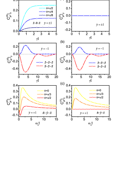
Figure 1: CPF correlation [Eq. (7)] for the deterministic and random schemes, left and right columns respectively, for equal measurement time intervals $t=\tau.$ (a) Eternal non-Markovianity, measurements $\hat{x}$-$\hat{n}$-$\hat{x}.$ (b) Decay in a bosonic bath, measurements $\hat{z}$-$\hat{z}$-$\hat{z}$ and $\hat{x}$-$\hat{z}$-$\hat{x}.$ (c) Dephasing in a bosonic bath, measurements $\hat{n}$-$\hat{y}$-$\hat{x}.$ In all cases, the $\hat{n}-$direction is defined by the angle $\theta.$ The renewed states $\rho_{\breve{y}=\pm 1}$ are described in the main text.

For the dissipative dynamics [$S=\left|{-}\right\rangle\left\langle{+}\right|$ in Eq. (19)] the CPF correlation in the random scheme reads unpublished

$$C_{pf}^{(r)}|_{\breve{y}=-1}\underset{\hat{z}\hat{z}\hat{z}}{=}|G(t,\tau)|^{2},\ \ \ \ \ C_{pf}^{(r)}|_{\breve{y}=-1}\underset{\hat{x}\hat{z}\hat{x}}{=}-\mathrm{Re}[G(t,\tau)].$$ (20)

Here, we consider two different measurement possibilities, $\hat{z}$-$\hat{z}$-$\hat{z}$ and $\hat{x}$-$\hat{z}$-$\hat{x}$ directions, both with conditional $\breve{y}=-1.$ The renewed states are $\rho_{\breve{y}=\pm}=|\pm\rangle\langle\pm|,$ and we take $\wp(\breve{y}|x)=1/2.$ The initial system state $|\psi_{0}\rangle$ is chosen such that $P(x)=1/2.$ Under this condition, for both measurement directions, in the deterministic scheme we get $C_{pf}^{(d)}|_{\breve{y}=-1}=[1-|G(t)|^{2}/2]^{-2}C_{pf}^{(r)}|_{\breve{y}=-1}.$ In these expressions, $G(t,\tau)\equiv\int_{0}^{t}dt^{\prime}\int_{0}^{\tau}d\tau^{\prime}f(\tau^{\prime}+t^{\prime})G(t-t^{\prime})G(\tau-\tau^{\prime}),$ where $G(t)$ is defined by the evolution$\ (d/dt)G(t)=-\int_{0}^{t}f(t-t^{\prime})G(t^{\prime})dt^{\prime},$ $G(0)=1.$ The memory kernel is the bath correlation $f(t)\equiv\sum_{k}|g_{k}|^{2}\exp[+i(\omega_{0}-\omega_{k})t].$

In Fig. 1(b), for a Lorentzian spectral density budiniBrasil , $f(t)=(\gamma/2\tau_{c})\exp(-|t|/\tau_{c}),$ with $\gamma\tau_{c}=5,$ we plot the CPF correlations. In contrast to the previous case, here for both the deterministic and random schemes, the CPF correlations do not vanish. Thus, memory effects rely on BIFs, which are present independently of the bath correlation time $\tau_{c}.$

In the dephasing case [$S=\sigma_{\hat{z}}$ in Eq. (19)], the CPF correlation in the random scheme is unpublished

$$C_{pf}^{(r)}|_{\breve{y}}\underset{\hat{n}\hat{y}\hat{x}}{=}\breve{y}\cos(\theta)\exp(-\gamma_{\tau})\sin(\Phi_{t,\tau}).$$ (21)

Here, we consider the successive measurements in Bloch directions $\hat{n}$-$\hat{y}$-$\hat{x}.$ Furthermore, we take $\wp(\breve{y}|x)=1/2,$ and pure states $\rho_{\breve{y}}$ corresponding to the eigenvectors of $\sigma_{\hat{y}}.$ The initial condition $|\psi_{0}\rangle$ is such that independently of $\hat{n},$ $P(x)=1/2.$ Under this condition the CPF correlation of the deterministic scheme can be written as $C_{pf}^{(d)}|_{\breve{y}}\underset{\hat{n}\hat{y}\hat{x}}{=}\sin(\theta)\exp[-(\gamma_{t}+\gamma_{t})]\sinh(\Gamma_{t,\tau})+C_{pf}^{(r)}|_{\breve{y}}.$ In these expressions, $\Gamma_{t,\tau}=\gamma_{t}+\gamma_{\tau}-\gamma_{t+\tau}$ and $\Phi_{t,\tau}=\phi_{t}+\phi_{\tau}-\phi_{t+\tau}$ where $\gamma_{t}\equiv 4\sum\nolimits_{k}(|g_{k}|^{2}/\omega_{k}^{2})[1-\cos(\omega_{k}t)],$ and $\phi_{t}\equiv 4\sum\nolimits_{k}(|g_{k}|^{2}/\omega_{k}^{2})\sin(\omega_{k}t).$

Assuming the spectral density $J(\omega)=\lambda\omega\exp(-\omega/\omega_{c}),$ where $\omega_{c}$ is a cutoff frequency breuerbook , it follows $\gamma_{t}=(1/2)\ln[1+(\omega_{c}t)^{2}]$ and $\phi_{t}=\arctan[\omega_{c}t]$ ($\lambda=1$). In Fig. 1(c) we plot the CPF correlation of both schemes. Even when the unperturbed system dynamics can be written as a (continuous) statistical superposition of unitary dynamics nori , our approach detects the presence of BIFs, $C_{pf}^{(r)}|_{\breve{y}}\neq 0.$ In fact, $C_{pf}^{(r)}|_{\breve{y}}=0$ only occurs for very specific measurement directions.

V Conclusions

Memory effects in open quantum systems may underlay or not on a bidirectional system-environment physical exchange of information. We introduced an operational scheme that allow to distinguishing between both situations, solving a long standing problem in the theory of non-Markovian open quantum systems. The method is based on a probabilistic relation that relates the developing of BIFs with the modification of the environmental dynamical behavior. We showed that BIFs can be detected with a minimal number of three system measurement processes added to an intermediate system update operation.

A generalized CPF correlation, defined between the first and last measurement outcomes, witnesses memory effects. Depending on the system state update scheme, deterministic vs. random, it witnesses memory effects independently of its underlying origin or restricted to the presence of BIFs respectively. Consistently, for environments modeled by classical noise fluctuations or when the environment dynamics (incoherent or quantum) is not affected during the system evolution, not any BIFs is detected. The presence of BIFs for decay and dephasing dynamics modeled through unitary system-environment interactions also support the consistence of the developed approach.

Given the operational character of the proposed scheme, it can be implemented, for example, in quantum optical arrangements budiniChina ; budiniBrasil , providing in general a valuable experimental tool for studying the underlying origin of quantum memory effects. Generalizations for an arbitrary number of measurement processes can also be worked out in a similar way. The proposed theoretical ground may also shed light on the possibility of classifying memory effects in classical and quantum ones costa , and may also provide an explicit test for different (causal) structures arising in quantum causal modelling causal .

Appendix A Joint probabilities

The system is subjected to three measurement processes performed at times $0\rightarrow t\rightarrow t+\tau.$ The corresponding measurement operators are denoted as $\{\Omega_{x}\},$ $\{\Omega_{y}\},$ and $\{\Omega_{z}\}.$ The intermediate $y$-measurement is taken as a projective one, $\Omega_{y}=|y\rangle\langle y|.$ The corresponding post-measurement system state is $\rho_{y}=|y\rangle\langle y|.$ After this step, the state transformation $\rho_{y}\rightarrow\rho_{\breve{y}}$ is externally applied. Each of the possible states $\{\rho_{\breve{y}}\}$ is chosen with conditional probability $\wp(\breve{y}|y,x),$ which only depends on the previous particular measurement outcomes $x$ and $y.$

The relevant joint probability $P(z,\breve{y},x)$ for the present proposal can be obtained as

$$P(z,\breve{y},x)=\sum_{y}P(z,\breve{y},y,x).$$ (22)

The joint probability for the four events $P(z,\breve{y},y,x)$ follows from standard quantum measurement theory after knowing the open system dynamics. The CPF probability $P(z,x|\breve{y}),$ which determine the CPF correlation [Eq. (7)] budiniCPF , can straightforwardly be obtained as

$$P(z,x|\breve{y})=P(z,\breve{y},x)/P(\breve{y}),$$ (23)

where $P(\breve{y})=\sum_{z,x}P(z,\breve{y},x)=\sum_{z,y,x}P(z,\breve{y},y,x).$ In addition, $P(z|\breve{y})=\sum_{x}P(z,x|\breve{y})$ and $P(x|\breve{y})=\sum_{z}P(z,x|\breve{y}).$

A.1 Classical noise environmental fluctuations

For classical noisy environments the outcomes probabilities are obtained for each realization, while an ensemble average is performed at the end of the calculation.

Let $\rho_{0}$ denotes the initial system state. After performing the first system measurement, with operators $\{\Omega_{x}\},$ it occurs the transformation $\rho_{0}\rightarrow\rho_{x},$ where

$$\rho_{x}=\frac{\Omega_{x}\rho_{0}\Omega_{x}^{\dagger}}{\mathrm{Tr}_{s}(E_{x}\rho_{0})}.$$ (24)

Here, $E_{x}=\Omega_{x}^{\dagger}\Omega_{x}.$ The probability of each outcome is

$$P(x)=\mathrm{Tr}_{s}(E_{x}\rho_{0}).$$ (25)

During the time interval$\ 0\rightarrow t,$ the system evolves with a (completely positive) dynamics defined by the stochastic propagator $\mathcal{E}_{t,0}^{st}.$ After the second $y$-measurement, with operators $\{\Omega_{y}\},$ it follows the transformation $\mathcal{E}_{t,0}^{st}[\rho_{x}]\rightarrow\rho_{y},$ where

$$\rho_{y}=\frac{\Omega_{y}\mathcal{E}_{t,0}^{st}[\rho_{x}]\Omega_{y}^{\dagger}}{\mathrm{Tr}_{s}(E_{y}\mathcal{E}_{t,0}^{st}[\rho_{x}])}=|y\rangle\langle y|,$$ (26)

and $E_{y}=\Omega_{y}^{\dagger}\Omega_{y}.$ Here, we used that the $y$-measurement is a projective one, $\Omega_{y}=|y\rangle\langle y|.$ The conditional probability $P^{st}(y|x)$ of outcome $y$ given that the previous one was $x$ is

$$P^{st}(y|x)=\mathrm{Tr}_{s}(E_{y}\mathcal{E}_{t,0}^{st}[\rho_{x}]).$$ (27)

At this stage, independently of the outcome $y,$ the system state is updated as $\rho_{y}\rightarrow\rho_{\breve{y}}.$ The states $\{\rho_{\breve{y}}\}$ are chosen with conditional probability $\wp(\breve{y}|y,x),$ which does not depend on the particular noise realization.

In the final steps $(t\rightarrow t+\tau),$ the system evolves with the propagator $\mathcal{E}_{t+\tau,t}^{st}$ and the last $z$-measurement, with operators $\{\Omega_{z}\},$ is performed ($\tau$ is the time interval between the measurements). Thus, $\mathcal{E}_{t+\tau,t}^{st}[\rho_{\breve{y}}]\rightarrow\rho_{z}^{st},$ where

$$\rho_{z}^{st}=\frac{\Omega_{z}\mathcal{E}_{t+\tau,t}^{st}[\rho_{\breve{y}}]\Omega_{z}^{\dagger}}{\mathrm{Tr}_{s}(E_{z}\mathcal{E}_{t+\tau,t}^{st}[\rho_{\breve{y}}])},$$ (28)

with $E_{z}=\Omega_{z}^{\dagger}\Omega_{z}.$ The conditional probability of outcome $z$ given that the previous ones were $x$ and $y,$ and given that the state $\rho_{\breve{y}}$ was imposed, is

$$P^{st}(z|\breve{y},y,x)=\mathrm{Tr}_{s}(E_{z}\mathcal{E}_{t+\tau,t}^{st}[\rho_{\breve{y}}]).$$ (29)

For each noise realization, this object does not depend on outcomes $y$ and $x.$

The joint probability of the four events $P(z,\breve{y},y,x)$ can be obtained as an average over an ensemble of realizations. Denoting the average operation with the overbar symbol, Bayes rule leads to

$$P(z,\breve{y},y,x)=\overline{P^{st}(z|\breve{y},y,x)\wp(\breve{y}|y,x)P^{st}(y|x)P(x)}.$$ (30)

From Eqs. (25), (27), and (29), we get

$$\frac{P(z,\breve{y},y,x)}{\wp(\breve{y}|y,x)}=\overline{\mathrm{Tr}_{s}(E_{z}\mathcal{E}_{t+\tau,t}^{st}[\rho_{\breve{y}}])\mathrm{Tr}_{s}(E_{y}\mathcal{E}_{t,0}^{st}[\tilde{\rho}_{x}])},$$ (31)

where $\tilde{\rho}_{x}\equiv\Omega_{x}\rho_{0}\Omega_{x}^{\dagger},$ which recovers Eq. (8).

A.2 Completely positive system-environment dynamics

Let $\rho_{0}^{se}=\rho_{0}\otimes\sigma_{0}$ denotes the bipartite state at the initial time. After performing the first system measurement, with operators $\{\Omega_{x}\},$ it occurs the transformation $\rho_{0}^{se}\rightarrow\rho_{x}^{se},$ where the post-measurement state is

$$\rho_{x}^{se}=\frac{\Omega_{x}\rho_{0}^{se}\Omega_{x}^{\dagger}}{\mathrm{Tr}_{se}(E_{x}\rho_{0}^{se})},$$ (32)

with $E_{x}=\Omega_{x}^{\dagger}\Omega_{x}.$ The probability of each outcome is

$$P(x)=\mathrm{Tr}_{s}(E_{x}\rho_{0}).$$ (33)

During the time interval$\ 0\rightarrow t,$ the bipartite arrangement evolves with a completely positive dynamics defined by the propagator $\mathcal{E}_{t,0}.$ After the second $y$-measurement, it follows the transformation $\mathcal{E}_{t,0}[\rho_{x}^{se}]\rightarrow\rho_{y}^{se},$ where

$$\rho_{y}^{se}=\frac{\Omega_{y}\mathcal{E}_{t,0}[\rho_{x}^{se}]\Omega_{y}^{\dagger}}{\mathrm{Tr}_{se}(E_{y}\mathcal{E}_{t}[\rho_{x}^{se}])}=\rho_{y}\otimes\sigma_{e}^{yx}.$$ (34)

Here, $E_{y}=\Omega_{y}^{\dagger}\Omega_{y}.$ In the last equality we used that the second measurement is a projective one, $\Omega_{y}=|y\rangle\langle y|$ and $\rho_{y}=|y\rangle\langle y|.$ The environment state is

$$\sigma_{e}^{yx}=\frac{\mathrm{Tr}_{s}(E_{y}\mathcal{E}_{t,0}[\rho_{x}^{se}])}{\mathrm{Tr}_{se}(E_{y}\mathcal{E}_{t,0}[\rho_{x}^{se}])}.$$ (35)

The conditional probability $P(y|x)$ of outcome $y$ given that the previous one was $x$ is

$$P(y|x)=\mathrm{Tr}_{se}(E_{y}\mathcal{E}_{t,0}[\rho_{x}^{se}]).$$ (36)

At this stage, independently of the outcome $y,$ the system is initialized in an independently chosen state $\rho_{\breve{y}},$ with conditional probability $\wp(\breve{y}|y,x).$ Thus, the bipartite state [Eq. (34)] becomes

$$\rho_{y}^{se}\rightarrow\rho_{\breve{y}}^{se}=\rho_{\breve{y}}\otimes\sigma_{e}^{yx}.$$ (37)

In the final steps $(t\rightarrow t+\tau),$ the bipartite system arrangement evolves with the propagator $\mathcal{E}_{t+\tau,t},$ and the last $z$-measurement is performed. Hence, $\mathcal{E}_{t+\tau,t}[\rho_{\breve{y}}\otimes\sigma_{e}^{yx}]\rightarrow\rho_{z}^{se},$ where

$$\rho_{z}^{se}=\frac{\Omega_{z}\mathcal{E}_{t+\tau,t}[\rho_{\breve{y}}\otimes\sigma_{e}^{yx}]\Omega_{z}^{\dagger}}{\mathrm{Tr}_{se}(E_{z}\mathcal{E}_{t+\tau,t}[\rho_{\breve{y}}\otimes\sigma_{e}^{yx}])},$$ (38)

with $E_{z}=\Omega_{z}^{\dagger}\Omega_{z}.$ The conditional probability of outcome $z$ given that the previous ones were $x$ and $y,$ and given that the state $\rho_{\breve{y}}$ was imposed, is

$$P(z|\breve{y},y,x)=\mathrm{Tr}_{se}(E_{z}\mathcal{E}_{t+\tau,t}[\rho_{\breve{y}}\otimes\sigma_{e}^{yx}]).$$ (39)

From Bayes rule, the joint probability $P(z,\breve{y},y,x)$ of the four events can be written as

$$P(z,\breve{y},y,x)=P(z|\breve{y},y,x)\wp(\breve{y}|y,x)P(y|x)P(x).$$ (40)

From Eqs. (33), (36), and (39), it follows

$$P(z,\breve{y},y,x) = \mathrm{Tr}_{se}(E_{z}\mathcal{E}_{t+\tau,t}[\rho_{\breve{y}}\otimes\sigma_{e}^{yx}])$$ (41)

$$\wp(\breve{y}|y,x)\mathrm{Tr}_{se}(E_{y}\mathcal{E}_{t,0}[\tilde{\rho}_{x}^{se}]),$$

where $\tilde{\rho}_{x}^{se}\equiv\Omega_{x}\rho_{0}^{se}\Omega_{x}^{\dagger}.$ Using Eq. (35) for $\sigma_{e}^{yx},$ finally we get

$$\frac{P(z,\breve{y},y,x)}{\wp(\breve{y}|y,x)}=\mathrm{Tr}_{se}(E_{z}\mathcal{E}_{t+\tau,t}[\rho_{\breve{y}}\otimes\mathrm{Tr}_{s}(E_{y}\mathcal{E}_{t,0}[\tilde{\rho}_{x}^{se}])]),$$ (42)

which recovers Eq. (11).

A.3 Unconditional environment average

The calculus of $P(z,\breve{y},y,x)$ in the previous section relies on the association $\langle\cdots\rangle_{\mathbf{e}}\leftrightarrow\mathrm{Tr}_{e}(\cdots).$ This unconditional environment average emerges when the the successive (non-selective) measurement of the environment do not modify its state at each stage. While this result follows straightforwardly from quantum measurement theory breuerbook , here it is explicitly confirmed.

We consider three measurement processes but now they provide information of both the system and the environment. The successive outcomes are denoted as $x\rightarrow(y\rightarrow\breve{y})\rightarrow z$ and $\mathfrak{X}\rightarrow\mathfrak{Y}\rightarrow\mathfrak{Z}$ (Latin and Fraktur letters) respectively. Introducing the notation $X=(x,\mathfrak{X}),$ $Y=(y,\mathfrak{Y}),$ and $Z=(z,\mathfrak{Z}),$ the measurement operators are denoted as $\{\Omega_{X}\},$ $\{\Omega_{Y}\},$ and $\{\Omega_{Z}\},$ where $\Omega_{X}=\Omega_{x}\otimes\Omega_{\mathfrak{X}},$ $\Omega_{Y}=\Omega_{y}\otimes\Omega_{\mathfrak{Y}}$ and $\Omega_{Z}=\Omega_{z}\otimes\Omega_{\mathfrak{Z}}.$ As before, the intermediate system measurement is taken as a projective one, $\Omega_{y}=|y\rangle\langle y|.$

From Bayes rule, the probability of all measurements and preparation events can be written as

$$P(Z,\breve{y},Y,X)=P(Z|\breve{y},Y,X)\wp(\breve{y}|y,x)P(Y|X)P(X).$$ (43)

By performing the same calculus steps as in the previous section, from Eqs. (41) straightforwardly we obtain

$$P(Z,\breve{y},Y,X) = \mathrm{Tr}_{se}(E_{Z}\mathcal{E}_{t+\tau,t}[\rho_{\breve{y}}\otimes\sigma_{e}^{YX}])$$ (44)

$$\wp(\breve{y}|y,x)\mathrm{Tr}_{se}(E_{Y}\mathcal{E}_{t,0}[\tilde{\rho}_{X}^{se}]),$$

where $E_{J}=\Omega_{J}^{\dagger}\Omega_{J}$ $(J=X,Y,Z),$ and $\tilde{\rho}_{X}^{se}=\Omega_{X}\rho_{0}^{se}\Omega_{X}^{\dagger}.$ Furthermore,

$$\sigma_{e}^{YX}=\frac{\Omega_{\mathfrak{Y}}\mathrm{Tr}_{s}(E_{y}\mathcal{E}_{t,0}[\rho_{X}^{se}])\Omega_{\mathfrak{Y}}^{{\dagger}}}{\mathrm{Tr}_{se}(E_{Y}\mathcal{E}_{t,0}[\rho_{X}^{se}])},$$ (45)

where $\rho_{X}^{se}=\tilde{\rho}_{X}^{se}/\mathrm{Tr}_{se}(E_{X}\rho_{0}^{se}).$ Similarly, Eq. (44) can be rewritten as

$$\!\frac{P(\!Z,\!\breve{y},\!Y,\!X\!)}{\wp(\breve{y}|y,x)}\!=\!\mathrm{Tr}_{se}(\!E_{Z}\mathcal{E}_{t+\tau,t}[\rho_{\breve{y}}\otimes\Omega_{\mathfrak{Y}}\mathrm{Tr}_{s}(E_{y}\mathcal{E}_{t,0}[\tilde{\rho}_{X}^{se}])\Omega_{\mathfrak{Y}}^{{\dagger}}]).$$ (46)

The probability for the environment outcomes follows by marginating the system outcomes,

$$P(\mathfrak{Z},\mathfrak{Y},\mathfrak{X})=\sum_{z,\breve{y},y,x}P(Z,\breve{y},Y,X).$$ (47)

Similarly, the probability for the system outcomes follows by marginating the outcomes corresponding to the reservoir measurements,

$$P(z,\breve{y},y,x)=\sum_{\mathfrak{Z},\mathfrak{Y},\mathfrak{X}}P(Z,\breve{y},Y,X).$$ (48)

This result for $P(z,\breve{y},y,x)$ relies on explicit environment measurements. In contrast, the results of the previous section were derived assuming that the environment is not observed at all. Nevertheless, both kind of results can be put in one-to-one correspondence. In fact, Eqs. (41) and (42) can be recovered from Eqs. (44) and (46), via the margination (48), under the conditions

$$\sigma_{0}=\sum_{\mathfrak{X}}\Omega_{\mathfrak{X}}\sigma_{0}\Omega_{\mathfrak{X}}^{{\dagger}},\ \ \ \ \ \ \ \sigma_{e}^{yx}=\sum_{\mathfrak{Y}}\Omega_{\mathfrak{Y}}\sigma_{e}^{yx}\Omega_{\mathfrak{Y}}^{{\dagger}},$$ (49)

where $\sigma_{0}$ is the initial bath state and $\sigma_{e}^{yx}$ is defined by Eq. (35). As expected, these equalities imply that the bath states at each stage are not modified by the corresponding reservoir (non-selective) measurement processes. Thus, the unconditional environment average of the previous section [Eq. (42)] relies on this kind of observables, which allow us to formulate the full approach without performing any explicit reservoir measurement.

For projective environment measurements, the relations (49) implies the commutation relations $[\sigma_{0},\Omega_{\mathfrak{X}}]=0,$ $[\sigma_{e}^{yx},\Omega_{\mathfrak{Y}}]=0.$ In classical (incoherent) reservoirs, where the bath state is diagonal in (a unique) privileged basis, these conditions define the corresponding “classical environment observables.”

Appendix B Eternal non-Markovianity

The non-Markovian system density matrix evolution is given by Eq. (17). There exist different underlying dynamic that lead to this dynamics. The solution map $\rho_{0}\rightarrow\rho_{t}$ can be written as a mixture of three Markovian maps megier

$$\rho_{t}=\sum_{\alpha=\hat{x},\hat{y},\hat{z}}q_{\alpha}\mathcal{E}_{t,0}^{(\alpha)}[\rho_{0}],$$ (50)

with positive and normalized statistical weights $\{q_{\alpha}\},$ $\sum_{\alpha=\hat{x},\hat{y},\hat{z}}q_{\alpha}=1.$ The Markovian propagators are

$$\mathcal{E}_{t,t_{0}}^{(\alpha)}[\rho_{0}]=h_{t-t_{0}}^{(+)}\rho_{0}+h_{t-t_{0}}^{(-)}\sigma_{\alpha}\rho_{0}\sigma_{\alpha},$$ (51)

with scalar functions $h_{t}^{(\pm)}\equiv(1\pm e^{-2\gamma t})/2.$ Each propagator $\mathcal{E}_{t,t_{0}}^{(\alpha)}=\exp[\gamma(t-t_{0})\mathbb{L}_{\alpha}]$ corresponds to the solution of the Markovian Lindblad evolution

$$\frac{d}{dt}=\gamma\mathbb{L}_{\alpha}[\rho_{t}]=\gamma(\sigma_{\alpha}\rho_{t}\sigma_{\alpha}-\rho_{t}).$$ (52)

The evolution (17) emerges with $q_{\hat{x}}=q_{\hat{y}}=1/2$ and $q_{\hat{z}}=0$ megier .

The probability $P(z,\breve{y},y,x)$ can be straightforwardly be obtained from Eq. (31) under the replacement $\overline{(\cdots)}\rightarrow\sum_{\alpha}q_{\alpha}\cdots.$ We get

$$\frac{P(z,\breve{y},y,x)}{\wp(\breve{y}|y,x)}=\!\sum_{\alpha=\hat{x},\hat{y},\hat{z}}\!\!\!q_{\alpha}\mathrm{Tr}_{s}(E_{z}\mathcal{E}_{t+\tau,t}^{(\alpha)}[\rho_{\breve{y}}])\mathrm{Tr}_{s}(E_{y}\mathcal{E}_{t,0}^{(\alpha)}[\tilde{\rho}_{x}]),$$ (53)

where $E_{i}\equiv\Omega_{i}^{\dagger}\Omega_{i}$ $(i=x,y,z)$ and $\tilde{\rho}_{x}\equiv\Omega_{x}\rho_{0}\Omega_{x}^{\dagger}$ is the (unnormalized) system state after the first $x$-measurement. $\mathrm{Tr}_{s}(\cdots)$ denotes a trace operation in the system Hilbert space. $\rho_{\breve{y}}$ is the (updated) system state after the second $y$-measurement.

In the deterministic scheme $[\wp(\breve{y}|y,x)=\delta_{\breve{y},y}],$ using that $P(z,\breve{y},x)=\sum_{y}P(z,\breve{y},y,x),$ Eq. (53) leads to

$$P(z,\breve{y},x)\overset{d}{=}\sum_{\alpha=\hat{x},\hat{y},\hat{z}}q_{\alpha}\mathrm{Tr}_{s}(E_{z}\mathcal{E}_{t+\tau,t}^{(\alpha)}[\rho_{\breve{y}}])\mathrm{Tr}_{s}(E_{\breve{y}}\mathcal{E}_{t,0}^{(\alpha)}[\tilde{\rho}_{x}]).$$ (54)

In general, this joint probability does not fulfill a Markov condition. Thus, $C_{pf}^{(d)}|_{\breve{y}}\neq 0$ detects memory effects. On the other hand, in the random scheme $[\wp(\breve{y}|y,x)=\wp(\breve{y}|x)]$ it follows

$$P(z,\breve{y},x)\overset{r}{=}\sum_{\alpha=\hat{x},\hat{y},\hat{z}}q_{\alpha}\mathrm{Tr}_{s}(E_{z}\mathcal{E}_{t+\tau,t}^{(\alpha)}[\rho_{\breve{y}}])\wp(\breve{y}|x)\mathrm{Tr}_{s}(\tilde{\rho}_{x}),$$ (55)

which recovers a Markovian structure, $P(z,\breve{y},x)=P(z|\breve{y})\wp(\breve{y}|x)P(x),$ with $P(z|\breve{y})=\sum_{\alpha=\hat{x},\hat{y},\hat{z}}q_{\alpha}\mathrm{Tr}_{s}(E_{z}\mathcal{E}_{t+\tau,t}^{(\alpha)}[\rho_{\breve{y}}])$ and $P(x)=\mathrm{Tr}_{s}(\tilde{\rho}_{x}).$ Thus, independently of the chosen system measurement observables it follows $C_{pf}^{(r)}|_{\breve{y}}=0,$ indicating consistently the absence of any BIF.

$\hat{x}$-$\hat{n}$-$\hat{x}$ measurements

We consider the case in which the three measurements are projective ones. The first and third ones are performed in $\hat{x}$-direction of the Bloch sphere. The intermediate one is performed in a direction $\hat{n}=\{\sin(\theta),0,\cos(\theta)\},$ which lies in the $\hat{x}$-$\hat{z}$ plane of the Bloch sphere. Thus, the measurement operators are $\Omega_{x=\pm}=|\hat{x}_{\pm}\rangle\langle\hat{x}_{\pm}|,$ $\Omega_{y=\pm}=|\hat{n}_{\pm}\rangle\langle\hat{n}_{\pm}|,$ and $\Omega_{z=\pm}=|\hat{x}_{\pm}\rangle\langle\hat{x}_{\pm}|.$ Consistently with the chosen directions, we have $|\hat{x}_{\pm}\rangle=(|+\rangle\pm|-\rangle)/\sqrt{2},$ jointly with $|\hat{n}_{+}\rangle=\cos(\theta/2)|+\rangle+\sin(\theta/2)|-\rangle,$ and $|\hat{n}_{-}\rangle=\sin(\theta/2)|+\rangle-\cos(\theta/2)|-\rangle.$

For an explicit calculation of the previous probabilities we need to calculate $P_{\alpha}(\hat{n}|\hat{x})\equiv\mathrm{Tr}_{s}(E_{\hat{n}}\mathcal{E}_{t_{f},t_{i}}^{(\alpha)}[\rho_{\hat{x}}])$ and $P_{\alpha}(\hat{x}|\hat{n})\equiv\mathrm{Tr}_{s}(E_{\hat{x}}\mathcal{E}_{t_{f},t_{i}}^{(\alpha)}[\rho_{\hat{n}}]),$ where $E_{\hat{n}}=|\hat{n}\rangle\langle\hat{n}|$ and $\rho_{\hat{x}}=|\hat{x}\rangle\langle\hat{x}|.$ From Eq. (51) and the definition of the measurement operators, we get

$$P_{\alpha}(\hat{n}|\hat{x})=P_{\alpha}(\hat{x}|\hat{n})=h_{t_{f}-t_{i}}^{(+)}|\langle\hat{n}|\hat{x}\rangle|^{2}+h_{t_{f}-t_{i}}^{(-)}|\langle\hat{n}|\sigma_{\alpha}|\hat{x}\rangle|^{2}.$$ (56)

Using this result, after a straightforward calculation, from Eqs. (54) and (56) we get

$$P(z,\breve{y},x)\overset{d}{=}\frac{1}{4}[1+\breve{y}x\sin(\theta)c(t)+z\breve{y}\sin(\theta)c(\tau)$$

$$\ \ \ \ \ \ \ \ \ \ \ \ \ \ \ \ \ \ +zx\sin^{2}(\theta)c(t+\tau)]P(x),$$ (57)

where $P(x)=\mathrm{Tr}_{s}(E_{x}\rho_{0}),$ and

$$c(t)\equiv q_{\hat{x}}+(q_{\hat{y}}+q_{\hat{z}})\exp[-2\gamma t].$$ (58)

In the random scheme, from Eq. (55) we obtain

$$P(z,\breve{y},x)\overset{r}{=}\frac{1}{2}[1+z\breve{y}\sin(\theta)c(\tau)]\wp(\breve{y}|x)P(x),$$ (59)

where we considered the updated states $\rho_{\breve{y}=\pm 1}=|\hat{n}_{\pm}\rangle\langle\hat{n}_{\pm}|.$

The generalized CPF correlation is given by Eq. (7), $C_{pf}^{(d/r)}|_{\breve{y}}=\sum_{zx}O_{z}O_{x}[P(z,x|\breve{y})-P(z|\breve{y})P(x|\breve{y})],$ where $P(z,x|\breve{y})$ follows from Eq. (23). Furthermore, $O_{z}=z=\pm 1$ and $O_{x}=x=\pm 1.$ From Eq. (57), the CPF correlation in the deterministic scheme reads

$$C_{pf}^{(d)}|_{\breve{y}}\underset{\hat{x}\hat{n}\hat{x}}{=}\sin^{2}(\theta)\frac{[1-\langle x\rangle^{2}]}{4[P(\breve{y})]^{2}}[c(t+\tau)-c(t)c(\tau)],$$ (60)

where $P(\breve{y})=(1/2)[1+\breve{y}\langle x\rangle\sin(\theta)c(t)]$ and $\langle x\rangle\equiv\sum_{x=\pm 1}xP(x).$ When $\rho_{0}=|\pm\rangle\langle\pm|$ it follows $P(x)=1/2$ and consequently $\langle x\rangle=0.$ This case recovers Eq. (18).

In the random scheme, from Eq. (59) consistently it follows

$$C_{pf}^{(r)}|_{\breve{y}}=0.$$ (61)

This equality is valid independently of the chosen measurement processes and updated system states [see Eq. (55)].

References

- (1) H. P. Breuer and F. Petruccione, The theory of open quantum systems, (Oxford University Press, 2002).
- (2) I. de Vega and D. Alonso, Dynamics of non-Markovian open quantum systems, Rev. Mod. Phys. 89, 015001 (2017).
- (3) L. Li, M. J. W. Hall, and H. M. Wiseman, Concepts of quantum non-Markovianity: A hierarchy, Phys. Rep. 759, 1 (2018).
- (4) H. P. Breuer, E. M. Laine, J. Piilo, and V. Vacchini, Colloquium: Non-Markovian dynamics in open quantum systems, Rev. Mod. Phys. 88, 021002 (2016).
- (5) A. Rivas, S. F. Huelga, and M. B. Plenio, Quantum non-Markovianity: characterization, quantification and detection, Rep. Prog. Phys. 77, 094001 (2014).
- (6) R. Schmidt, S. Maniscalco, and T. Ala-Nissila, Heat flux and information backflow in cold environments, Phys. Rev. A 94, 010101(R) (2016); S. H. Raja, M. Borrelli, R. Schmidt, J. P. Pekola, and S. Maniscalco, Thermodynamic fingerprints of non-Markovianity in a system of coupled superconducting qubits, Phys. Rev. A 97, 032133 (2018).
- (7) G. Guarnieri, C. Uchiyama, and B. Vacchini, Energy backflow and non-Markovian dynamics, Phys. Rev. A 93, 012118 (2016).
- (8) G. Guarnieri, J. Nokkala, R. Schmidt, S. Maniscalco, and B. Vacchini, Energy backflow in strongly coupled non-Markovian continuous-variable systems, Phys. Rev. A 94, 062101 (2016).
- (9) S. Cialdi, C. Benedetti , D. Tamascelli, S. Olivares, M. G. A. Paris, and B. Vacchini, Experimental investigation of the effect of classical noise on quantum non-Markovian dynamics, Phys. Rev. A 100, 052104 (2019).
- (10) J. I. Costa-Filho, R. B. B. Lima, R. R. Paiva, P. M. Soares, W. A. M. Morgado, R. Lo Franco, and D. O. Soares-Pinto, Enabling quantum non-Markovian dynamics by injection of classical colored noise, Phys. Rev. A 95, 052126 (2017).
- (11) J. Trapani and M. G. A. Paris, Nondivisibility versus backflow of information in understanding revivals of quantum correlations for continuous-variable systems interacting with fluctuating environments, Phys. Rev. A 93, 042119 (2016); C. Benedetti, F. Buscemi, P. Bordone, and M. G. A. Paris, Non-Markovian continuous-time quantum walks on lattices with dynamical noise, Phys. Rev. A 93, 042313 (2016).
- (12) J. Trapani, M. Bina, S. Maniscalco, and M. G. A. Paris, Collapse and revival of quantum coherence for a harmonic oscillator interacting with a classical fluctuating environment, Phys. Rev. A 91, 022113 (2015); T. Grotz, L. Heaney, and W. T. Strunz, Quantum dynamics in fluctuating traps: Master equation, decoherence, and heating, Phys. Rev. A 74, 022102 (2006); A. A. Budini, Quantum systems subject to the action of classical stochastic fields, Phys. Rev. A 64, 052110 (2001).
- (13) H. P. Breuer, Non-Markovian generalization of the Lindblad theory of open quantum systems, Phys. Rev. A 75, 022103 (2007); A. A. Budini, Lindblad rate equations, Phys. Rev. A 74, 053815 (2006).
- (14) B. Vacchini, Non-Markovian dynamics for bipartite systems, Phys. Rev. A 78, 022112 (2008).
- (15) A. A. Budini, Post-Markovian quantum master equations from classical environment fluctuations, Phys. Rev. E 89, 012147 (2014).
- (16) C. Sutherland, T. A. Brun, and D. A. Lidar, Non-Markovianity of the post-Markovian master equation, Phys. Rev. A 98, 042119 (2018); A. Shabani and D. A. Lidar, Completely positive post-Markovian master equation via a measurement approach, Phys. Rev. A 71, 020101(R) (2005).
- (17) B. Donvil, P. Muratore-Ginanneschi, and J. P. Pekola, Hybrid master equation for calorimetric measurements, Phys. Rev. A 99, 042127 (2019).
- (18) B. Vacchini, Non-Markovian master equations from piecewise dynamics, Phys. Rev. A 87, 030101(R) (2013).
- (19) A. A. Budini, Embedding non-Markovian quantum collisional models into bipartite Markovian dynamics, Phys. Rev. A 88, 032115 (2013); A. A. Budini and P. Grigolini, Non-Markovian nonstationary completely positive open-quantum-system dynamics, Phys. Rev. A 80, 022103 (2009); A. A. Budini, Stochastic representation of a class of non-Markovian completely positive evolutions, Phys. Rev. A 69, 042107 (2004).
- (20) D. Chruściński and F. A. Wudarski, Non-Markovian random unitary qubit dynamics, Phys. Lett. A 377, 1425 (2013); D. Chruściński and F. A. Wudarski, Non-Markovianity degree for random unitary evolution, Phys. Rev. A 91, 012104 (2015); F. A. Wudarski, P. Nalezyty, G. Sarbicki, and D. Chruściński, Admissible memory kernels for random unitary qubit evolution, Phys. Rev. A 91, 042105 (2015); F. A. Wudarski and D. Chruściński, Markovian semigroup from non-Markovian evolutions, Phys. Rev. A 93, 042120 (2016); K. Siudzińska and D. Chruściński, Memory kernel approach to generalized Pauli channels: Markovian, semi-Markov, and beyond, Phys. Rev. A 96, 022129 (2017).
- (21) C. M. Kropf, C. Gneiting, and A. Buchleitner, Effective Dynamics of Disordered Quantum Systems, Phys. Rev. X 6, 031023 (2016); C. Gneiting, F. R. Anger, and A. Buchleitner, Incoherent ensemble dynamics in disordered systems, Phys. Rev. A 93, 032139 (2016).
- (22) H.-B. Chen, C. Gneiting, P.-Y. Lo, Y.-N. Chen, and F. Nori, Simulating Open Quantum Systems with Hamiltonian Ensembles and the Nonclassicality of the Dynamics, Phys. Rev. Lett. 120, 030403 (2018).
- (23) B. Paredes, F. Verstraete, and J. I. Cirac, Exploiting Quantum Parallelism to Simulate Quantum Random Many-Body Systems, Phys. Rev. Lett. 95, 140501 (2005).
- (24) H. P. Breuer, E. M. Laine, and J. Piilo, Measure for the Degree of Non-Markovian Behavior of Quantum Processes in Open Systems, Phys. Rev. Lett. 103, 210401 (2009).
- (25) M. M. Wolf, J. Eisert, T. S. Cubitt, and J. I. Cirac, Assessing Non-Markovian Quantum Dynamics, Phys. Rev. Lett. 101, 150402 (2008).
- (26) A. Rivas, S. F. Huelga, and M. B. Plenio, Entanglement and Non-Markovianity of Quantum Evolutions, Phys. Rev. Lett. 105, 050403 (2010).
- (27) E. -M. Laine, J. Piilo, and H. -P. Breuer, Measure for the non-Markovianity of quantum processes, Phys. Rev. A 81, 062115 (2010).
- (28) X.-M. Lu, X. Wang, and C. P. Sun, Quantum Fisher information flow and non-Markovian processes of open systems, Phys. Rev. A 82, 042103 (2010).
- (29) A. K. Rajagopal, A. R. Usha Devi, and R. W. Rendell, Kraus representation of quantum evolution and fidelity as manifestations of Markovian and non-Markovian forms, Phys. Rev. A 82, 042107 (2010).
- (30) D. Chruściński, A. Kossakowski, and A. Rivas, Measures of non-Markovianity: Divisibility versus backflow of information, Phys. Rev. A 83, 052128 (2011).
- (31) S. Luo, S. Fu, and H. Song, Quantifying non-Markovianity via correlations, Phys. Rev. A 86, 044101 (2012).
- (32) S. Lorenzo, F. Plastina, and M. Paternostro, Geometrical characterization of non-Markovianity, Phys. Rev. A 88, 020102(R) (2013).
- (33) D. Chruściński and S. Maniscalco, Degree of Non-Markovianity of Quantum Evolution, Phys. Rev. Lett. 112, 120404 (2014).
- (34) F. F. Fanchini, G. Karpat, B. Çakmak, L. K. Castelano, G. H. Aguilar, O. Jiménez Farías, S. P. Walborn, P. H. Souto Ribeiro, and M. C. de Oliveira, Non-Markovianity through Accessible Information, Phys. Rev. Lett. 112, 210402 (2014).
- (35) C. Addis, G. Brebner, P. Haikka, and S. Maniscalco, Coherence trapping and information backflow in dephasing qubits, Phys. Rev. A 89, 024101 (2014).
- (36) M. J. W. Hall, J. D. Cresser, L. Li, and E. Andersson, Canonical form of master equations and characterization of non-Markovianity, Phys. Rev. A 89, 042120 (2014).
- (37) P. Haikka, J. D. Cresser, and S. Maniscalco, Comparing different non-Markovianity measures in a driven qubit system, Phys. Rev. A 83, 012112 (2011). C. Addis, B. Bylicka, D. Chruściński, and S. Maniscalco, Comparative study of non-Markovianity measures in exactly solvable one- and two-qubit models, Phys. Rev. A 90, 052103 (2014).
- (38) B. Bylicka, M. Johansson, and A. Acín, Constructive Method for Detecting the Information Backflow of Non-Markovian Dynamics, Phys. Rev. Lett. 118, 120501 (2017).
- (39) S. Chakraborty, Generalized formalism for information backflow in assessing Markovianity and its equivalence to divisibility, Phys. Rev. A 97, 032130 (2018); S. Chakraborty and D. Chruscinski, Information flow versus divisibility for qubit evolution, Phys. Rev. A 99, 042105 (2019).
- (40) J. Kołodynski, S. Rana, and A. Streltsov, Entanglement negativity as a universal non-Markovianity witness, Phys. Rev. A 101, 020303(R) (2020).
- (41) A. Norambuena, J. R. Maze, P. Rabl, and R. Coto, Quantifying phonon-induced non-Markovianity in color centers in diamond, Phys. Rev. A 101, 022110 (2020).
- (42) B.-H. Liu, L. Li, Y.-F. Huang, C. F. Li, G. C. Guo, E.-M. Laine, H.-P. Breuer, and J. Piilo, Experimental control of the transition from Markovian to non-Markovian dynamics of open quantum systems, Nat. Phys. 7, 931 (2011).
- (43) M. Wittemer, G. Clos, H. P. Breuer, U. Warring, and T. Schaetz, Measurement of quantum memory effects and its fundamental limitations, Phys. Rev. A 97, 020102(R) (2018).
- (44) D. F. Urrego, J. Flórez, J. Svozilík, M. Nuñez, and A. Valencia, Controlling non-Markovian dynamics using a light-based structured environment, Phys. Rev. A 98, 053862 (2018).
- (45) D. Khurana, B. K. Agarwalla, and T. S. Mahesh, Experimental emulation of quantum non-Markovian dynamics and coherence protection in the presence of information backflow, Phys. Rev. A 99, 022107 (2019).
- (46) S.-J. Xiong, Q. Hu, Z. Sun, L. Yu, Q. Su, J.-M. Liu, and C.-P. Yang, Non-Markovianity in experimentally simulated quantum channels: Role of counterrotating-wave terms, Phys. Rev. A 100, 032101 (2019).
- (47) A. Cuevas, A. Geraldi, C. Liorni, L. D. Bonavena, A. De Pasquale, F. Sciarrino, V. Giovannetti, and P. Mataloni, All-optical implementation of collision-based evolutions of open quantum systems, Sci. Rep. 9, 3205 (2019).
- (48) Y.-N. Lu ,Y.-R. Zhang, G.-Q. Liu , F. Nori, H. Fan, and X.-Y. Pan, Observing Information Backflow from Controllable Non-Markovian Multichannels in Diamond, Phys. Rev. Lett. 124, 210502 (2020).
- (49) N. Megier, D. Chruściński, J. Piilo, and W. T. Strunz, Eternal non-Markovianity: from random unitary to Markov chain realisations, Sci. Rep. 7, 6379 (2017).
- (50) A. A. Budini, Maximally non-Markovian quantum dynamics without environment-to-system backflow of information, Phys. Rev. A 97, 052133 (2018).
- (51) A. Smirne, M. Caiaffa, and J. Piilo, Rate Operator Unraveling for Open Quantum System Dynamics, Phys. Rev. Lett. 124, 190402 (2020).
- (52) F. A. Pollock, C. Rodríguez-Rosario, T. Frauenheim, M. Paternostro, and K. Modi, Operational Markov Condition for Quantum Processes, Phys. Rev. Lett. 120, 040405 (2018); F. A. Pollock, C. Rodríguez-Rosario, T. Frauenheim, M. Paternostro, and K. Modi, Non-Markovian quantum processes: Complete framework and efficient characterization, Phys. Rev. A 97, 012127 (2018).
- (53) P. Taranto, F. A. Pollock, S. Milz, M. Tomamichel, and K. Modi, Quantum Markov Order, Phys. Rev. Lett. 122, 140401 (2019); P. Taranto, S. Milz, F. A. Pollock, and K. Modi, Structure of quantum stochastic processes with finite Markov order, Phys. Rev. A 99, 042108 (2019).
- (54) M. R. Jørgensen and F. A. Pollock, Exploiting the Causal Tensor Network Structure of Quantum Processes to Efficiently Simulate Non-Markovian Path Integrals, Phys. Rev. Lett. 123, 240602 (2019).
- (55) Y. -Y. Hsieh, Z. -Y. Su, and H. -S. Goan, Non-Markovianity, information backflow, and system-environment correlation for open-quantum-system processes, Phys. Rev. A 100, 012120 (2019).
- (56) A. A. Budini, Quantum Non-Markovian Processes Break Conditional Past-Future Independence, Phys. Rev. Lett. 121, 240401 (2018); A. A. Budini, Conditional past-future correlation induced by non-Markovian dephasing reservoirs, Phys. Rev. A 99, 052125 (2019).
- (57) S. Yu, A. A. Budini, Y. -T. Wang, Z. -J. Ke, Y. Meng, W. Liu, Z. -P. Li, Q. Li, Z. -H. Liu, J. -S. Xu, J. -S. Tang, C. -F. Li , and G. -C. Guo, Experimental observation of conditional past-future correlations, Phys. Rev. A 100, 050301(R) (2019).
- (58) T. de Lima Silva, S. P. Walborn, M. F. Santos, G. H. Aguilar, and A. A. Budini, Detection of quantum non-Markovianity close to the Born-Markov approximation, Phys. Rev. A 101, 042120 (2020).
- (59) M. Bonifacio and A. A. Budini, Perturbation theory for operational quantum non-Markovianity, Phys. Rev. A 102, 022216 (2020).
- (60) L. Han, J. Zou, H. Li, and B. Shao, Non-Markovianity of A Central Spin Interacting with a Lipkin–Meshkov–Glick Bath via a Conditional Past–Future Correlation, Entropy 22, 895 (2020).
- (61) In fact, from Bayes rule where jointly with and
- (62) Formally, the update is equivalent to discard the system state and feeds forward an independent system state. Named as “repreparation,” this operation was introduced in Ref. pollock for studying “quantum Markov order.” The formulation with unitary transformations defines a feasible experimental implementation.
- (63) Under the condition the invariance property (14) is fulfilled only when the initial bath state satisfies
- (64) A. A. Budini, unpublished.
- (65) C. Giarmatzi and F. Costa, Witnessing quantum memory in non-Markovian processes, arXiv:1811.03722v3.
- (66) F. Costa and S. Shrapnel, Quantum causal modelling, New J. Phys. 18, 063032 (2016); A. Feix and C. Brukner, Quantum superpositions of ‘common-cause’ and ‘direct-cause’ causal structures, New J. Phys. 19, 123028 (2017).