Testing Scalable Bell Inequalities for Quantum Graph States
on IBM Quantum Devices

Abstract

Testing and verifying imperfect multi-qubit quantum devices are important as such noisy quantum devices are widely available today. Bell inequalities are known useful for testing and verifying the quality of the quantum devices from their nonlocal quantum states and local measurements. There have been many experiments demonstrating the violations of Bell inequalities but they are limited in the number of qubits and the types of quantum states. We report violations of Bell inequalities on IBM Quantum devices based on the scalable and robust inequalities maximally violated by graph states as proposed by Baccari et al. (Ref.[1]). The violations are obtained from the quantum states of path graphs up to 57 and 21 qubits on the 65-qubit and 27-qubit IBM Quantum devices, respectively, and from those of star graphs up to 8 and 7 qubits with error mitigation on the same devices. We are able to show violations of the inequalities on various graph states by constructing low-depth quantum circuits producing them, and by applying the readout error mitigation technique. We also point out that quantum circuits for star graph states of size $N$ can be realized with circuits of depth $O(\sqrt{N})$ on subdivided honeycomb lattices which are the topology of the 65-qubit IBM Quantum device. Our experiments show encouraging results on the ability of existing quantum devices to prepare entangled quantum states, and provide experimental evidences on the benefit of scalable Bell inequalities for testing them.

I Introduction

Nonlocality of quantum states–first discovered by John S. Bell [2]–is an intriguing consequence of quantum mechanics in which correlations among quantum bits cannot be explain by classical statistics. In particular, the nonlocality implies the so-called Bell inequalities that are violated by entangled (or, nonlocal) quantum states but not by any classical (or, local) correlation. There is a variety of concepts and experimental tools developed for demonstrating the violation of Bell inequalities [3]. One of them is the CHSH inequality [4],that can be used to test the nonlocality of two quantum bits. There have been many researches extending the CHSH inequality, such as that by Ito, Imai, and Avis [5] whose inequality allows wider range of quantum states to violate the classical bounds, or the CHSH-like Bell inequalities for more-than-two quantum bits, such as, the Mermin’s inequality for Greenberger–Horne–Zeilinger (GHZ) state [6] and the Bell inequality for graph states [7].

The Bell inequalities soon find their applications for witnessing entanglement [8, 9] and for self-testing [10, 11] quantum devices. The latter is useful for certifying the quantumness of the devices by statistical tests on the correlations resulting from the quantum states they produce without the knowledge of their internal functions. However, most of the existing Bell inequalities require measuring correlations on quantum graph states whose number scales exponentially [12, 7] or polynomially [13, 14, 15] with the number of qubits involved. Recently, Baccari et al. [1] proposed a family of CHSH-like Bell inequalities that are both scalable and robust. The scalability comes from the fact that the new inequalities can be tested by measuring correlations on quantum graph states whose number scales only linearly with the number of qubits. The robustness stems from the fact that the maximal violation is obtained from quantum graph states whose ratio of the quantum bound against the classical bound tends to a constant for sufficiently large number of qubits. In addition, the fidelity of the violating quantum states against the corresponding quantum graph states is a linear function of the magnitude of the violations. The scalability and robustness of the new CHSH-like Bell inequalities are therefore potential for self-testing noisy quantum devices available today.

We have been witnessing the proliferation of near-term quantum devices [16, 17, 18, 19, 20]. As in January 2021 there are at least seventeen multi-qubit quantum devices made available at IBM Quantum Experience . Although far from perfect, their number and quality of the qubits has been much improved since the first introduction of their predecessor in 2016. The quantum devices with the largest number of qubits is the 65-qubit (ibmq_manhattan) followed by other smaller devices. The quality of those devices is measured with the Quantum Volume [22, 16] which is a single metric incorporating the number of qubits and the depth of the quantum circuits applicable to the qubits before they decohere. Those devices offer testbeds for investigating the quantum states they produce, i.e., to see if such topologically-limited noisy devices can entangle more qubits and in which way. For example, Wei et al. [23] experimentally demonstrated the ability to produce GHZ states up to 18 qubits on a 20-qubit IBM Quantum device measured by their proposed scalable entanglement metric. González et al. [24] and Huang et al. [25] used Mermin-type Bell inequalities to confirm entanglement of GHZ states up to 5 qubits. Nevertheless, the previous experiments are limited and are also difficult to verify different types of entangled quantum states that may depend on the underlying quantum devices.

We address the task of testing noisy quantum devices with various quantum graph states based on the the family of CHSH-like Bell inequalities of Baccari et al. [1]. We exploit their Bell inequalities to construct various inequalities based on the qubit layout topology of the underlying quantum devices. The inequalities are maximally violated by quantum graph states, whose graphs can be varied based on the connectivity of the qubits of the devices. In particular, we construct path and star graphs on the 65-qubit ibmq_manhattan, 27-qubit ibmq_toronto, and ibmq_sydney devices and test their violations of the corresponding Bell inequalities. For path graphs the inequalities are clearly violated on the longest simple paths available on the quantum devices: up to 57 qubits on the 65-qubit device, and up to 21 qubits on the 27-qubit devices. For star graphs the violations are observed up to 7 qubits on ibmq_manhattan and 8 qubits on ibmq_sydney and ibmq_toronto after applying the measurement error mitigation based on tensor product noise model (Recently, Mooney et al. independently verified 27-qubit GHZ states in a different way to us [26]).

We also checked violations of the inequalities on graphs corresponding to the underlying devices, i.e., all 65 qubits of the ibmq_manhattan, and 27 qubits of ibmq_toronto and ibmq_sydney, and we report the violation on ibmq_manhattan.

The violations are made possible by shallow-depth circuits to produce the corresponding graph states. Namely, path graphs are from depth-2 quantum circuits as in [27], and star graphs on 5 qubits or larger are from quantum circuits avoiding SWAP gates following a similar construction shown in [23]. We provide a generalization of constructing star graph states of $N$ qubits with circuits of depth $O(\sqrt{N})$ on subdivided honeycomb lattices which are the typical topology of IBM Quantum devices.

The rest of the paper is organized as follows. Section II explains the experimental settings by introducing the graph states, the corresponding CHSH-like Bell inequalities and the quantum circuits producing the graph states. Section III shows the experimental results on IBM Quantum devices showing their ability to entangle more qubits than reported before. Section IV concludes with the discussion of the results and future works.

II Settings of Experiments

In this section, we describe the settings and procedures of our experiments which were implemented on IBM Quantum Experience. The device information (calibration data) of each quantum device we used is listed in the Appendix B.

II.1 Preliminaries of Graph State

First, we consider a graph $G=(V,E)$ is a simple undirected graph with vertex set $V=\{1,2,\cdots,N\}$ and edge set $E=\{\{u,v\}|u,v\in V,u\neq v\}$. Let $n(v)$ be the vertex set of neighbourhoods of the vertex $v$ and $n[v]:=n(v)\cup\{v\}$ be the vertex set containing neighbourhoods of the vertex $v$ and $v$ itself. Given a graph $G=(V,E)$, the graph state $\ket{\psi_{G}}$ associated to the graph $G=(V,E)$ is defined in the following way. To every vertex $v$, $G_{v}$ is an operator on $N$-qubit system written as

$$\begin{aligned} G_{v}=\sigma_{X}^{(v)}\otimes\bigotimes_{i\in n(v)}\sigma_{Z}^{(i)},\end{aligned}$$ (1)

where the Pauli operator $\sigma_{X}^{(j)}$ or $\sigma_{Z}^{(j)}$ acts on the qubit $j$. Then the graph state $\ket{\psi_{G}}$ associated to $G$ is defined to be the unique simultaneous eigenvector,

$$\begin{aligned} \left|\psi_{G}\right\rangle:=\prod_{(i,j)\in E}CZ(i,j)|+\rangle^{\otimes N}.\end{aligned}$$ (2)

We can prepare the quantum circuit of graph state $\ket{\psi_{G}}$ using the formula (2).

II.2 The Scalable Bell Inequality of Baccari et al.

In order to review the scalable Bell inequality of Baccari et al. used in our experiment, we refer to their original notations in [1]. The inequality we used is the modified version of their original inequality, which is also mentioned in [1]. Using the notation of stabilizer measurement (1), the general form of their modified inequality becomes (3).

$$\begin{aligned} I_{G}(F)=&\sum_{v\in F}\left(\operatorname{deg}(v)\left\langle G_{v}\right\rangle+\sum_{i\in n(v)}\left\langle G_{i}\right\rangle\right)\\ +&\sum_{i\notin\bigcup_{v\in F}n[v]}\left\langle G_{i}\right\rangle\leq\beta_{G}^{C}(F)\end{aligned}$$ (3)

where $\beta_{G}^{C}(F)$ represents the classical bound of graph $G$ to the choice of $F$. In addition, $F$ satisfies ${}^{\forall}u,v\in F,\ n[u]\cap n[v]=\emptyset$. We also define $\beta_{G}^{Q}(F)$ as the quantum bound of $G$.

In our experiments, we computed $I_{G}(F)$ in (3) for path graph states, where the choice of elements for $F$ was optimized in order to obtain higher ratio of $\beta_{G}^{Q}/\beta_{G}^{C}$. For star graphs, $I_{G}(F)$ becomes quite simpler and it is described as the following form (4).

$$I_{S_{N}}=\sqrt{2}\left((N-1)\left\langle\sigma_{X}^{(1)}\sigma_{Z}^{(2)}\cdots\sigma_{Z}^{(N)}\right\rangle+\sum_{i\in V\backslash\{1\}}\left\langle\sigma_{Z}^{(1)}\sigma_{X}^{(i)}\right\rangle\right)$$

(4)

II.3 Circuit Preparation

In this experiment, we investigated the correlations of path graph $P_{N}$ and star graph $S_{N}$ using the IBM Quantum 65-qubit device (ibmq_manhattan) and 27-qubit devices (ibmq_toronto and ibmq_sydney). In order to make shallower circuits for path graph state, star graph state, and the quantum state of the graph structure inherent to each real device, we referred to the circuit designing techniques used by Wei et al. [23] and Mooney et al. [27].

II.3.1 Preparing Path Graph State

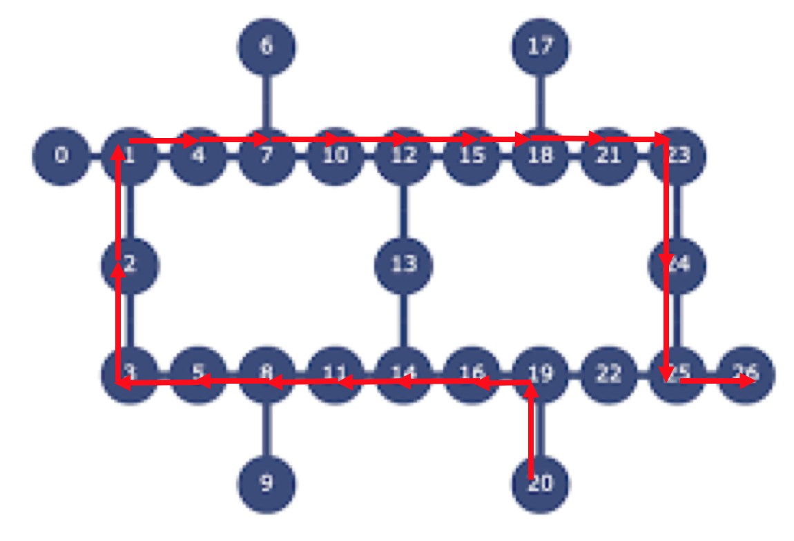
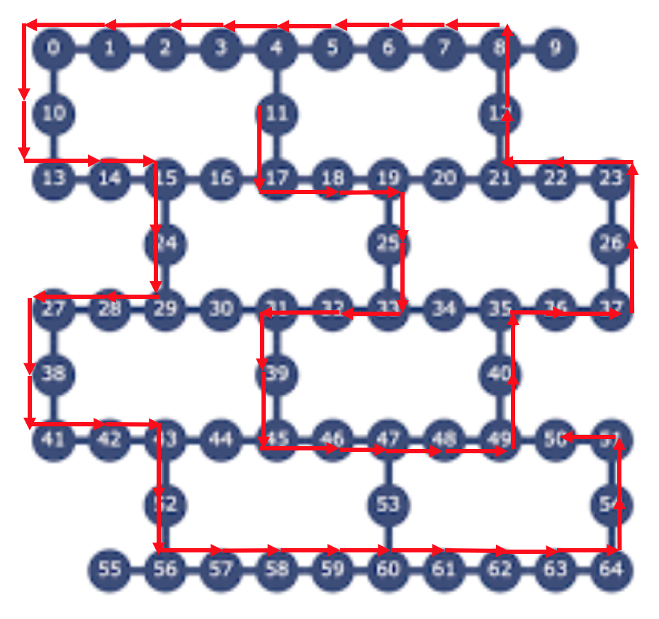
Figure 3: The qubit layout of path graph on ibmq_sydney and ibmq_toronto is shown at the left figure. Starting from qubit 20, we extend the path through the red arrows for each size of the graph until qubit 26 (max length: 21). The qubit layout on ibmq_manhattan is at the right figure. For ibmq_manhattan, we start from qubit 11 and finally reach qubit 50 (max length: 57).

Path graph state $\ket{\psi_{P_{N}}}$ can be prepared by shallow circuit with constant depth 2, as shown in [27]. Once we have prepared $\ket{+}^{\otimes N}$ state, we apply control-Z gate to every other edge of the path. Then we apply control-Z gate to every other remaining edge on which the control-Z gate was not applied at the previous step. We used the qubit layout in Fig. 3 in Appendix C in order to make as long paths as possible on each device. We tested path graph states from the size 2 up to the maximum size that can be taken on each devices.

II.3.2 Preparing Star Graph State

We can make star graphs from GHZ state by applying local Hadamard gate to its qubits except for the qubit representing the central node in the graph. That is, assuming that the central vertex is labled by $1$, then the following relashonship holds.

$$\begin{aligned} \ket{\psi_{S_{N}}}=\left(I\otimes H^{\otimes(N-1)}\right)\ket{\psi_{GHZ_{N}}}\end{aligned}$$ (5)

Then the remaining task is to prepare GHZ state. We can create GHZ state by using the technique shown in [23]. We will briefly review the idea of this method.

Since the qubits of entangled part of GHZ state, which are in the superposition state of $\ket{0}$ and $\ket{1}$, are all equivalent, we can choose the control qubit of the next target qubit from vertex $1$ to any preferable entangled vertex. In this sense, any tree graph structure is suitable for preparing GHZ state. In addition, by properly choosing the control qubit, we can apply in parallel the control-NOT gates to different pairs of qubits. By doing so, it is possible to realize shallower circuit with depth $O(\sqrt{N})$ for star graph state with size $N$ on the topology of IBM Quantum 65-qubit devices. In-depth discussion on the proof of this depth order on the topology of ibmq_manhattan is in the Appendix A.

In our experiments, we prepared the star graph $\ket{\psi_{S_{N}}}$ of size $N=1,\cdots,39$ on ibmq_manhattan, and of size $N=1,\cdots,27$ on ibmq_toronto and ibmq_sydney. The details on how we prepared star graphs on each devices is shown in Fig. 4 in Appendix C.

Besides, the grouping of observables with separable measurements, which has been conventionally used, would allow us to realize a fewer circuits and save resources of quantum computers. The idea of this technique is to firstly measure the sum of commutative observables at once, then extract the expectation value of each observable, and finally sum them up. For star graphs, since $\sigma_{Z}^{(1)}\sigma_{X}^{(i)}$ and $\sigma_{Z}^{(1)}\sigma_{X}^{(j)}$ are commutative, we substitute $n-1$ measurements in the term $\sum_{i\in V\backslash\{1\}}\left\langle\sigma_{Z}^{(1)}\sigma_{X}^{(i)}\right\rangle$ at (4) with one measurement $\sigma_{Z}^{(1)}\prod_{i\in{n(1)}}\sigma_{X}^{(i)}=\sigma_{Z}^{(1)}\sigma_{X}^{(2)}\cdots\sigma_{X}^{(N-1)}$. Using this technique, the number of quantum circuit for a star graph $S_{N}$ can be reduced into 2. By Hoeffding’s inequality, the number of shots for each circuits scales in $O\left(\frac{n^{2}}{\delta^{2}}\right)$, where $\delta$ is the error tolerance. In this sense, 8192 shots per circuit is enough for the size of qubits in our experiments.

II.3.3 Preparing the Graph Structure of Each Device

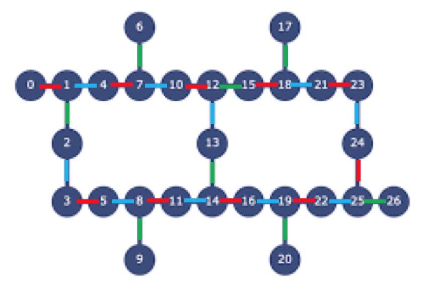
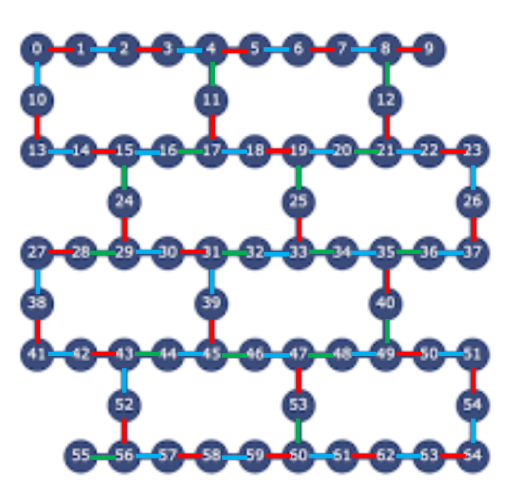
Figure 5: In order to prepare the subdivided honeycomb graph using the whole qubits in ibmq_toronto,ibmq_sydney, and ibmq_manhattan, we firstly apply control-Z gate on the red edges, then on the blue edges, and finally on the green edges. The ”focused” qubits in the inequality are [1,6,8,12,17,19,23,26] for ibmq_toronto and ibmq_sydney, and [3,6,9,10,17,21,24,25,26,31,35,38,44,47,54,56,59,62] for ibmq_manhattan.

The graph structure of qubit connection of each quantum devices we used can be seen as a subdivision of honeycomb graph. Let us define this graph of size $N$ as $TH_{N}$. Since the maximum degree of $TH_{N}$ is 3, it is shown to be 3-edge colorable. Therefore, we can prepare the quantum circuit for $TH_{N}$ in circuit depth 3. The specific construction of $TH_{N}$ corresponding to graph structure of each device is explained on Fig.5 of Appendix C.

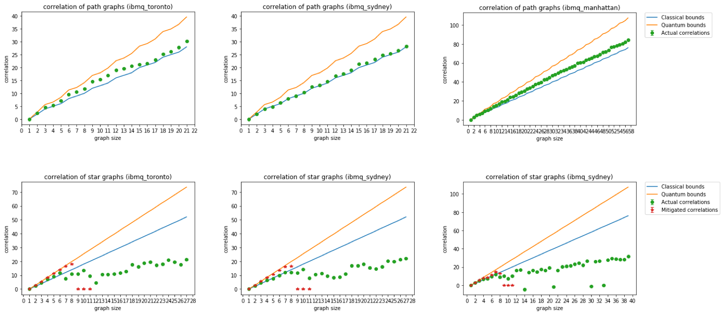
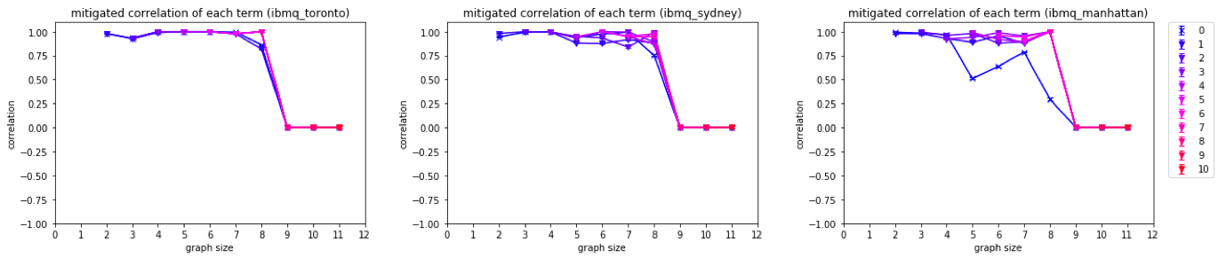
Figure 1: The correlations of path graphs and star graphs on each quantum devices. The upper row is the results of path graphs and the lower is of star graphs.

Figure 2: The term-wise correlations to different star graphs on each quantum devices after measurement error mitigation. For example, the correlation of the first term $\left\langle\sigma_{X}^{(1)}\sigma_{Z}^{(2)}\cdots\sigma_{Z}^{(N)}\right\rangle$ in (4) is represented as line 0 in each figure. For ibmq_toronto and ibmq_sydney, the depth changes between graph size 2-3, 4-5, 7-8, 10-11, 13-14, 17-18, 21-22, and 25-26. For ibmq_manhattan, the depth changes between graph size 2-3, 4-5, 7-8, 11-12, 16-17, 23-24, and 32-33.

III Results of Experiments

The results of quantum correlation for star graphs and path graphs on each device are shown in Fig. 2. The experiments are performed with Qiskit [20]. The result of each experiment is averaged over 8192 shots. The green plots are the correlations without error mitigation and the red plots are the correlations with the measurement error mitigation based on tensor product noise model. We added some modification to the tensored mitigation tool in qiskit-ignis library by our own, and applied it to star graph states up to size 11.

Fig. 2 shows the term wise mitigated correlations in (4) for each size of star graphs. For example, the curve labeled by 0 indicates the correlation of the term $\left\langle\sigma_{X}^{(0)}\sigma_{Z}^{(1)}\cdots\sigma_{Z}^{(N-1)}\right\rangle$ in (4) for graph size $N=2,3,4,\cdots$, and the curve labeled by 3 indicates the correlation of the term $\left\langle\sigma_{X}^{(0)}\sigma_{Z}^{(3)}\right\rangle$ in (4) for graph size $N=4,5,6,\cdots$.

From Fig. 2, we see path graphs violated the inequality with clear gap from classical bounds on ibmq_manhattan and ibmq_toronto, while for some small sizes of path graphs on ibmq_sydney did not violate. The curve for path graphs on each device seems to grow stably with the length of the path between the classical bound and quantum bound. Therefore, for path graphs, we may say they are well prepared on each device.

As for star graphs, we can see the violation of classical bound up to size 6 on ibmq_toronto and 7 on ibmq_sydney and ibmq_manhattan without error mitigation. When we added the measurement error mitigation to our raw results, the maximum size of star graph violating the classical bound increases to 8 on ibmq_toronto and ibmq_sydney, while the maximum size on ibmq_manhattan is still at 7. The decrease of total correlation from the size 4 to 5 and 7 to 8 at the plot of ibmq_manhattan probably reflects the increase of circuit depth, which would make each qubit more vulnerable to decoherence caused by the thermal relaxations.

We also report the violation of the CHSH-like Bell inequality by Baccari et al. in the subdivided honeycomb graph using whole qubits on ibmq_manhattan. The correlations of honeycomb struture on the devices of ibmq_toronto, ibmq_sydney, and ibmq_manhattan are listed in Table 1. This result implies that the ibmq_manhattan device has the ability to prepare a large graph state unique to its qubit layout even using its whole qubits, in rather good accuracy. For both ibmq_toronto and ibmq_sydney, the honeycomb structures on these two devices did not violate the classical bound of the inequality.

Table 1: The correlation values of whole-qubit honeycomb graph on each device, where $\overline{\beta}^{Q}_{G}$ denotes the measured quantum correlations.

ibmq_	toronto	sydney	manhattan
$\beta^{C}_{G}$	$36.000$	$36.000$	$88.000$
$\beta^{Q}_{G}$	$50.083$	$50.083$	$121.966$
$\overline{\beta}^{Q}_{G}$	$29.995\pm 0.094$	$33.241\pm 0.091$	$90.298\pm 0.1243$

The python codes of our experiments are stored at https://github.com/BOBO1997/qip2021_poster549.

IV Conclusion

Through our experiments, we support the benefits of the CHSH-like inequality proposed by Baccari et al. [1] in terms of its scalability and robustness. The linear-scale increase of measurement terms to the growth of graph size enables us to compute correlation of large graph states on IBM Quantum devices such as ibmq_manhattan with 65-qubits. Bell inequalities that require measuring only constant number of correlations [8, 9] have been used for experimenting with much larger systems [12, 28].

Using their remarkable Bell inequality, we also support the ability of existing IBM Quantum devices to prepare a well-entangled large graph states on them. We report in this work the violation of the inequality for several graph states with a large number of qubits. Using shallow circuits with depth 2 [27], we have seen path graphs violated the inequality up to the maximum size on each IBM Quantum device. In particular, for the IBM Quantum 65-qubit device, path graphs showed its quantumness up to size 57. We also checked the violation of classical bounds for the graph state corresponding to the graph structure of each quantum devices with its whole qubits. Although the maximum size of star graphs violating the inequality 3 is rather small compared to the violations in path graphs, our result reports the violation of star graphs up to size 7. Our preliminary efforts applying measurement error mitigation showed that the size could be increased up to 8.

For future works, one of the possible improvements of circuit preparation can be found in the experiments by Wei et al. [23]. During their experiments, they added a collective $\pi$-pulse on all qubits in order to refocus low frequency noise and reduces dephasing errors using the idea of Hahn echo [29]. As they applied the $\pi$-pulse between the entangle process and disentangle process of GHZ states which undo the entangle process, $\pi$-pulse becomes most effective for certain time intervals decided by T1/T2 relaxation times. Since our experiments do not have the structure of symmetry in terms of entangle process and disentangle process, partial insertion of $\pi$-pulse into the entangled qubits might improve the correlations instead of the direct insertion of $\pi$-pulse into the middle of our circuits. Other ideas of decreasing the dephasing errors, such as dynamic decoupling methods discussed in [30], might also help us improve the total correlations of the inequality.

In addition, other scalable measurement calibration techniques might further improve our results. One of the better measurement mitigation techiniques is the continuous time Marcov process (CTMP) measurement error mitigation recently proposed by Bravyi et al. [31]. This method takes account for the two qubits cross-talk errors and it is a generalization of tensor product noise model we used.

In conclusion, our results for the large quantum states greatly owe to the scalability of the Bell inequality proposed by Baccari et al. [1] and we experimentally support the usefulness of their inequality as a powerful tool for the entanglement verification of large quantum states and for the benchmarking of upcoming near-term quantum devices.

Appendix A Creating Star Graphs with Depth $O(\sqrt{N})$

At the previous part, we have seen that quantum circuit for star graph state $\ket{\psi_{S_{N}}}$ is prepared via the GHZ state which can avoid using the swap operations. Here we explain why the quantum circuit can be prepared with depth $O(\sqrt{N})$ for star graph $S_{N}$ on the physical qubit layout of ibmq_manhattan. We first describe the construction of tree graph state $\ket{\psi_{T_{N}}}$ with depth $d$ and see what the physical qubit topology should be taken. We then show such a graph can be embedded into the topology of subdivided honeycomb structure.

In order to create circuit, we start from vertex $1$. If vertex $1$ is connected with other vertex, say vertex $2$, we can add it to the tree, making $\ket{\psi_{T_{2}}}$ with depth $1$. Next, if one of the vertices $1,2$ has degree 3 or larger, connected with vertex $3$, and the other vertex has degree 2 or larger, connected with vertex $4$, then we can simultaneously add vertices $3,4$ to vertex $1,2$. This time, the created tree $\ket{\psi_{T_{4}}}$ has the depth $2$, with 3 outer vertices on the qubit topology connected to different vertices of $\ket{\psi_{T_{4}}}$. Going one step further, if two of three neighbourhoods of $\ket{\psi_{T_{4}}}$ have degree 2 or larger, and the remaining one neighbourhood has degree 3 or larger, then we can make $\ket{\psi_{T_{7}}}$ in one step, and assure 4 additional neighbourhoods for $\ket{\psi_{T_{7}}}$. In this way, the size of tree graph state we can prepare in depth $d$ is $N=\frac{1}{2}d(d+1)+1$. The condition that the physical qubit topology should satisfy is that they can add $d-1$ vertices with degree 2, and at least 1 vertex with degree $3$. Such structure can be found in subdivided honeycomb because every vertex with degree 2 in subdivided honeycomb is adjacent to vertices with degree 3, and vice versa.

Appendix B Device Information

Table 2: Qubit parameters on ibmq_toronto. The qubit frequency, T1, T2, readout error are presented.

Qubit	Frequency (GHz)	T1 (µs)	T2 (µs)	Readout error
0	5.225	104.4	59.0	0.0795
1	5.003	104.9	134.0	0.0611
2	5.144	63.6	138.4	0.016
3	5.21	97.1	159.4	0.0079
4	5.088	113.3	165.9	0.0469
5	5.167	97.7	131.5	0.0127
6	5.152	100.9	74.0	0.0224
7	4.915	126.5	167.7	0.0344
8	5.033	128.6	131.8	0.0129
9	5.082	107.2	103.4	0.0164
10	5.098	91.9	122.9	0.0326
11	5.117	28.4	62.5	0.0215
12	4.928	127.6	175.1	0.0476
13	5.128	100.2	127.8	0.2522
14	5.017	84.9	172.1	0.0116
15	5.092	116.0	56.3	0.2024
16	4.943	108.2	149.4	0.0329
17	5.158	107.6	74.9	0.0171
18	5.06	95.6	142.0	0.0644
19	5.069	99.9	123.8	0.0212
20	4.916	117.6	10.5	0.0108
21	5.145	50.0	31.8	0.0133
22	5.122	115.9	137.6	0.0219
23	5.1	126.2	43.3	0.0428
24	4.963	140.2	146.9	0.0099
25	5.065	156.5	182.1	0.0117
26	5.216	86.5	112.2	0.0122

Table 3: Qubit parameters on ibmq_sydney. The qubit frequency, T1, T2, readout error are presented.

Qubit	Frequency (GHz)	T1 (µs)	T2 (µs)	Readout error
0	5.092	35.5	40.3	0.0296
1	5.014	93.0	39.5	0.0599
2	4.863	126.7	55.5	0.0165
3	5.104	78.1	54.6	0.0231
4	5.064	70.0	89.2	0.0129
5	4.893	142.3	66.6	0.0148
6	4.994	79.8	107.4	0.0478
7	4.943	80.4	78.2	0.0565
8	4.761	192.8	131.1	0.0428
9	4.85	74.7	98.3	0.0332
10	5.047	72.8	118.5	0.0104
11	4.847	77.9	90.3	0.0769
12	5.0	88.3	43.8	0.0356
13	4.882	120.8	137.1	0.0173
14	5.097	85.6	153.7	0.0604
15	4.761	113.3	108.5	0.0173
16	4.968	89.9	52.0	0.0173
17	5.054	103.8	30.9	0.0759
18	4.895	75.0	25.0	0.0866
19	4.894	123.9	90.5	0.0264
20	5.026	89.6	172.2	0.073
21	4.943	89.1	36.2	0.0697
22	4.985	100.6	157.6	0.0479
23	5.071	107.5	149.7	0.0242
24	4.969	100.4	117.6	0.0402
25	4.891	99.2	219.4	0.1005
26	5.021	119.8	143.1	0.0217

Table 4: Qubit parameters on ibmq_manhattan. The qubit frequency, T1, T2, readout error are presented.

Qubit	Frequency (GHz)	T1 (µs)	T2 (µs)	Readout error
0	4.838	65.6	98.7	0.0338
1	4.681	65.9	73.2	0.0165
2	4.947	63.8	94.3	0.0137
3	4.766	52.0	71.4	0.0097
4	4.71	44.3	52.7	0.014
5	4.574	60.3	40.9	0.0323
6	4.758	57.2	97.8	0.0162
7	4.63	69.4	107.2	0.022
8	4.778	43.9	57.0	0.0221
9	4.929	89.8	107.1	0.0168
10	4.688	56.7	80.6	0.0169
11	4.764	66.6	109.2	0.0284
12	4.939	59.4	94.7	0.0135
13	4.84	52.7	48.7	0.0202
14	4.624	48.8	5.8	0.1513
15	4.803	52.0	54.7	0.0453
16	4.649	60.6	17.3	0.0113
17	4.877	55.5	68.6	0.0221
18	4.817	45.7	72.9	0.0126
19	4.999	44.4	77.3	0.0145
20	4.843	46.7	16.6	0.035
21	4.78	66.5	81.4	0.0129
22	4.935	79.5	104.6	0.0174
23	4.797	26.2	52.0	0.0351
24	5.012	68.3	48.7	0.0239
25	4.859	37.7	46.5	0.0198
26	4.721	67.2	85.0	0.0168
27	4.8	68.7	87.8	0.0273
28	4.896	21.8	37.2	0.0164
29	4.786	79.6	87.7	0.0165
30	4.89	69.9	52.4	0.0113
31	5.03	52.7	75.9	0.0135
32	4.898	71.8	92.2	0.0289
33	4.647	65.8	91.1	0.0165
34	4.781	53.0	73.7	0.0093
35	4.697	68.7	71.6	0.0346
36	4.971	66.9	107.7	0.0118
37	4.811	71.3	95.8	0.0081
38	4.97	64.3	79.7	0.0502
39	4.8	67.0	28.7	0.0093
40	4.545	90.5	129.7	0.0177
41	4.801	61.8	81.5	0.0159
42	4.663	56.1	92.7	0.0209
43	4.781	31.9	26.5	0.0592
44	4.683	85.7	117.9	0.0177
45	4.931	63.8	90.1	0.0188
46	4.799	65.5	90.3	0.0081
47	4.885	55.6	90.1	0.0121
48	4.758	52.6	77.8	0.0109
49	4.661	42.9	53.2	0.0905
50	4.782	44.1	71.0	0.022
51	4.887	44.9	74.4	0.0246
52	4.899	71.2	54.2	0.0234
53	4.677	63.2	88.3	0.0158
54	4.703	59.9	92.7	0.054
55	4.881	68.9	94.7	0.0254
56	4.795	54.6	76.7	0.0291
57	4.618	58.1	82.4	0.0325
58	4.784	64.7	89.6	0.0103
59	4.925	50.4	67.7	0.0261
60	4.777	69.4	98.2	0.0069
61	4.641	79.3	94.9	0.0148
62	4.826	54.1	13.2	0.0212
63	4.698	11.2	21.1	0.0443
64	4.832	71.9	24.0	0.0136

Appendix C Qubit Layouts

Figure 4: The range of sizes for star graphs with different circuit depth is painted with different colors. Each area of red, orange, yellow, green, cyan, blue, purple represents the range of circuit depth from 1 to 8 respectively. We expand the star graph from qubit 8 on ibmq_toronto and ibmq_sydney (max size: 27), and from qubit 33 on ibmq_manhattan (max size: 39).