Gel’fand’s inverse problem for the graph Laplacian

Abstract

We study the discrete Gel’fand’s inverse boundary spectral problem of determining a finite weighted graph. Suppose that the set of vertices of the graph is a union of two disjoint sets: $X=B\cup G$, where $B$ is called the set of the boundary vertices and $G$ is called the set of the interior vertices. We consider the case where the vertices in the set $G$ and the edges connecting them are unknown. Assume that we are given the set $B$ and the pairs $(\lambda_{j},\phi_{j}|_{B})$, where $\lambda_{j}$ are the eigenvalues of the graph Laplacian and $\phi_{j}|_{B}$ are the values of the corresponding eigenfunctions at the vertices in $B$. We show that the graph structure, namely the unknown vertices in $G$ and the edges connecting them, along with the weights, can be uniquely determined from the given data, if every boundary vertex is connected to only one interior vertex and the graph satisfies the following property: any subset $S\subseteq G$ of cardinality $|S|\geqslant 2$ contains two extreme points. A point $x\in S$ is called an extreme point of $S$ if there exists a point $z\in B$ such that $x$ is the unique nearest point in $S$ from $z$ with respect to the graph distance. This property is valid for several standard types of lattices and their perturbations.

1.  Introduction

In this paper, we consider the discrete version of Gel’fand’s inverse boundary spectral problem, defined for a finite weighted graph and the graph Laplacian on it. We assume that we are given the Neumann eigenvalues of the graph Laplacian and the values of the corresponding Neumann eigenfunctions at a pre-designated subset of vertices, called the boundary vertices.

Gel’fand’s inverse boundary spectral problem was originally formulated in [42] for partial differential equations. For partial differential operators, one considers an $n$-dimensional Riemannian manifold $(M,g)$ with boundary and the Neumann eigenvalue problem

$$-\Delta_{g}\Phi_{j}(x)=\omega_{j}\Phi_{j}(x),\quad\text{for }x\in M,$$ (1.1)

$$\ \ \partial_{\nu}\Phi_{j}|_{\partial M}=0,\quad$$ (1.2)

where $\Delta_{g}$ is the Laplace–Beltrami operator with respect to the Riemannian metric $g$ on $M$, and $\Phi_{j}:M\to\mathbb{R}$ are the eigenfunctions corresponding to the eigenvalues $\omega_{j}\in\mathbb{R}$. In local coordinates $(x^{i})_{i=1}^{n}$, the Laplacian has the representation

$$\Delta_{g}u={\rm det}(g)^{-\frac{1}{2}}\sum_{i,j=1}^{n}\frac{\partial}{\partial x^{i}}\left({\rm det}(g)^{\frac{1}{2}}g^{ij}\frac{\partial}{\partial x^{j}}u\right),$$ (1.3)

where $g(x)=[g_{ij}(x)]_{i,j=1}^{n}$, ${\rm det}(g)={\rm det}(g_{ij}(x))$ and $[g^{ij}]^{n}_{i,j=1}=g(x)^{-1}$.

Gel’fand’s inverse problem is to find the topology, differential structure and Riemannian metric of $(M,g)$ when one is given the boundary $\partial M$ and the pairs $(\omega_{j},\Phi_{j}|_{\partial M}),$ $j=1,2,\dots$, where $\omega_{j}$ are the Neumann eigenvalues and $\Phi_{j}|_{\partial M}$ are the Dirichlet boundary values of the corresponding eigenfunctions. Here, the eigenfunctions $\Phi_{j}$ are assumed to form a complete orthonormal family in $L^{2}(M)$. We review earlier results on this problem and the related problems in Section 1.2.

To formulate the discrete Gel’fand’s inverse problem, we consider a finite weighted graph. We use the following terminology. When $X$ is the set of vertices of a finite graph, we can declare any subset $B\subseteq X$ to be the set of the boundary vertices, denoted by $B=\partial G$, and call the set $G=X{{-}}B$ the set of the interior vertices of $X$. This terminology is motivated by inverse problems where one typically aims to reconstruct objects in a set $\Omega\subseteq\mathbb{R}^{n}$ using observations on the boundary $\partial\Omega$. In our case, we aim to reconstruct objects in a vertex set $G\subseteq X$ from observations on the boundary $\partial G$.

For $x,y\in X={{G}}\cup\partial{{G}}$, we denote $x\sim y$ if there is an edge in the edge set $E$ connecting $x$ to $y$, that is, $\{x,y\}\in E$. Every edge $\{x,y\}\in E$ has a weight $g_{xy}=g_{yx}>0$ and every vertex $x\in{{G}}$ has a measure $\mu_{x}>0$. For a function $u:{{G}}\cup\partial{{G}}\to\mathbb{R}$ defined on the whole vertex set, the graph Laplacian $\Delta_{G}$ on ${{G}}$ is defined by

$$\big{(}\Delta_{G}u\big{)}(x)=\frac{1}{\mu_{x}}\sum_{\begin{subarray}{c}y\sim x\\ y\in G\cup\partial G\end{subarray}}g_{xy}\big{(}u(y)-u(x)\big{)},\quad x\in{{G}},$$ (1.4)

and the Neumann boundary value $\partial_{\nu}u$ of $u$ is defined by

$$\big{(}\partial_{\nu}u\big{)}(z)=\frac{1}{\mu_{z}}\sum_{\begin{subarray}{c}x\sim z\\ x\in G\end{subarray}}g_{xz}\big{(}u(x)-u(z)\big{)},\quad z\in\partial G.$$ (1.5)

We consider the Neumann eigenvalue problem

$$-\Delta_{G}\phi_{j}(x)=\lambda_{j}\phi_{j}(x),\quad\text{for }x\in{{G}},$$ (1.6)

$$\ \ \partial_{\nu}\phi_{j}|_{\partial{{G}}}=0.$$ (1.7)

The discrete Gel’fand’s inverse problem is to find the set of interior vertices ${{G}}$, the edge structure of $({{G}}\cup\partial{{G}},E)$ and the weights $g,\mu$, when one is given the boundary $\partial G$ and the pairs $(\lambda_{j},\phi_{j}|_{\partial G}),$ $j=1,2,\dots,N$, $N=|G|$, where $|G|$ is the number of elements in $G$. Here, $\{\phi_{j}\}_{j=1}^{N}$ is a complete orthonormal family of eigenfunctions and their Dirichlet boundary values, $\phi_{j}|_{\partial G}=\big{(}\phi_{j}(z)\big{)}_{z\in\partial G}$, are vectors in $\mathbb{R}^{|\partial G|}$.

We mention that with suitable choices of $g,\mu$, our definition of the graph Laplacian (1.4) includes widely used Laplacians in graph theory, in particular, the combinatorial Laplacian when $g,\mu\equiv 1$, and the normalized Laplacian when $g\equiv 1,\,\mu_{x}=\textrm{deg}(x)$. The spectra of these two particular operators are mostly unrelated for general graphs and were usually studied separately.

Solving the discrete Gel’fand’s inverse problem is not possible without further assumptions due to the existence of isospectral graphs, see [35, 40, 68]. One of the main difficulties we encounter in solving the problem is that the graph Laplacian can have nonzero eigenfunctions which vanish identically on a part of the graph. This phenomenon, intuitively caused by the symmetry of the graph, can make one part of the graph invisible to the spectral data measured at another part. Therefore one needs to impose appropriate assumptions. On one hand, the assumptions have to break some symmetry of the graph to make the inverse problem solvable, and also designate sufficiently many boundary vertices to measure data on. On the other, the assumptions need to include a large class of interesting graphs besides trees, since trees are already well-understood. In this paper, we introduce the Two-Points Condition (1), and prove that the inverse boundary spectral problem on finite graphs is solvable with this assumption. Our result can be applied to detect local perturbations and recover potential functions on periodic lattices ([3, 4]), in particular, to probe graphene defects from the scattering matrix. We will address potential applications in another work.

We start by defining the notations for undirected simple graphs, where weights on vertices and edges are considered. These weights are related to physical situations where graph models are applicable.

1.1 Finite graphs

A graph is generally denoted by a pair $(X,E)$ with $X$ being the set of vertices and $E$ being the set of edges between vertices. A graph $(X,E)$ is finite if both $X$ and $E$ are finite. A graph is said to be simple if there is at most one edge between any pair of vertices and no edge between the same vertex. For undirected simple graphs, edges are two-element subsets of $X$. We endow a general graph with the following additional structures that affect wave propagation on the graph.

Definition 1.1 (Weighted graph with boundary).

We say that $\mathbb{G}=(G,\partial G,E,\mu,g)$ is a weighted graph with boundary if the following conditions are satisfied.

• $G\cup\partial G$ is the set of vertices (points), $G\cap\partial G=\emptyset$; $E$ is the set of edges. Elements of $G$ are called interior vertices and elements of $\partial G$ are called boundary vertices. We require $(G\cup\partial G,E)$ to be an undirected simple graph.

• $\mu:G\cup\partial G\to\mathbb{R}_{+}$ is the weight function on the set of vertices.

• $g:E\to\mathbb{R}_{+}$ is the weight function on the set of edges.

We use the following terminology. A graph with boundary $\mathbb{G}$ is finite if $(G\cup\partial G,E)$ is finite. Vertices $x$ and $y$ are adjacent, denoted by $x\sim y$, if $\{x,y\}\in E$, i.e., there is an edge connecting $x$ to $y$. When $x\sim y$, we denote by $g_{xy}$, or equivalently $g_{yx}$, the weight of the edge connecting $x$ to $y$. We write $\mu_{x}$ short for $\mu(x)$.

The degree of a vertex $x$ of $\mathbb{G}$ is defined as the number of vertices connected to $x$ by edges in $E$, denoted by $\deg_{E}(x)$ or $\deg_{\mathbb{G}}(x)$. The neighbourhood $N(\partial G)$ of $\partial G$ is defined by

$$N(\partial G)=\{x\in G:x\sim z\textrm{ for some }z\in\partial G\}\cup\partial G.$$

When the weights are not relevant in a specific context, we make use of the notation $(G,\partial G,E)$ for an unweighted graph with boundary.

Definition 1.2 (Paths and metric).

Let $x,y\in G\cup\partial G$. A path of $(G\cup\partial G,E)$ from $x$ to $y$ is a sequence of vertices $(v_{j})_{j=0}^{J}$ satisfying $v_{0}=x$, $v_{J}=y$ and $v_{j}\sim v_{j+1}$ for $j=0,\ldots,J-1$. The length of the path is $J$. The distance between $x$ and $y$, denoted by $d(x,y)$, is the minimal length among all paths from $x$ to $y$. In other words, the distance $d(x,y)$ is the minimal number of edges in paths that connect $x$ to $y$. The distance is defined to be infinite if there is no path from $x$ to $y$. An undirected graph $(G\cup\partial G,E)$ can be considered as a discrete metric space equipped with the distance function $d$. An undirected graph is connected if there exists a path between any pair of vertices.

A graph with boundary $\mathbb{G}$ is said to be connected if $(G\cup\partial G,E)$ is connected. We say that $\mathbb{G}$ is strongly connected, if it is still connected after one removes all edges connecting boundary vertices to boundary vertices (see Definition 2.4).

We remark that in our setting, any pair of adjacent vertices has distance $1$, while different choices of distances appear in other settings. If the graph sits in a manifold, it is more natural to use the intrinsic distance of the underlying manifold. For this type of graphs, additionally with geometric choices of weights, the graph Laplacian (1.4) can be used to approximate the standard Laplacians on the manifold, as long as the graphs are sufficiently dense ([20, 21, 22, 59]).

Definition 1.3.

Given a subset $S\subseteq G$, we say a point $x_{0}\in S$ is an extreme point of $S$ with respect to $\partial G$, if there exists a point $z\in\partial G$ such that $x_{0}$ is the unique nearest point in $S$ from $z$, with respect to the distance $d$ on $(G\cup\partial G,E)$.

Assumption 1.

We impose the following assumptions on the finite graph $(G,\partial G,E)$.

1. For any subset $S\subseteq G$ with cardinality at least $2$, there exist at least two extreme points of $S$ with respect to $\partial G$. We refer to this condition as the Two-Points Condition.

2. For any $z\in\partial G$ and any pair of distinct points $x,y\in G$, if $x\sim z,\,y\sim z$, then $x\sim y$.

Note that Item 2 of 1 is void if every boundary point is connected to only one interior point. Hence any graph can be adjusted to satisfy Item 2 by attaching an additional edge to every boundary point and declaring the added vertices as the new boundary points. We remark that Item 2 is essential for proper wavefront behaviour (see Lemma 3.5).

One can view the Two-Points Condition (Item 1 of 1) as a criterion of choosing appropriate boundary points for solving the inverse boundary spectral problem. As an intuitive example in the continuous setting, any compact subset of a square in $\mathbb{R}^{2}$ has at least two extreme points unless it is a single point set. In this case, two extreme points can be chosen by taking a point achieving the maximal height and a point achieving the minimal height with respect to one edge of the square. The boundary points realizing the extreme point condition are the vertical projections of those two chosen points to the proper edges (see Figure 1). Several types of graphs satisfying the Two-Points Condition are discussed in Section 1.3.

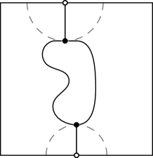
Figure 1: Any non-singleton compact subset of the unit square in $\mathbb{R}^{2}$ has at least two extreme points with respect to the boundary of the square.

From now on, let $\mathbb{G}$ be a finite weighted graph with boundary. For a function $u:G\cup\partial G\to\mathbb{R}$, its graph Laplacian on $G$ is defined by the formula (1.4). Recall that the Neumann boundary value of $u$ is defined by the formula (1.5), see e.g. [26, 30]. For $u_{1},u_{2}:G\cup\partial G\to\mathbb{R}$, we define the $L^{2}(G)$-inner product by

$$\langle u_{1},u_{2}\rangle_{L^{2}(G)}=\sum_{x\in G}\mu_{x}u_{1}(x)u_{2}(x).$$ (1.8)

For a finite graph with boundary, the function space $L^{2}(G)$ is exactly the space of real-valued functions on $G\cup\partial G$ equipped with the inner product (1.8). Note that the inner product is calculated only on the interior $G$ and not on the boundary $\partial G$. The main reason for such consideration is that we mostly deal with functions $u$ satisfying $\partial_{\nu}u|_{\partial G}=0$, in which case the values of $u$ on $\partial G$ are uniquely and linearly determined by the values on $G$, see (3.2).

Let $q:G\to\mathbb{R}$ be a potential function, and we consider the following Neumann eigenvalue problem for the discrete Schr$\ddot{\textrm{o}}$dinger operator $-\Delta_{G}+q$.

$$\begin{cases}(-\Delta_{G}+q)u(x)=\lambda u(x),&x\in G,\lambda\in\mathbb{R},\\ \partial_{\nu}u|_{\partial G}=0\,.\end{cases}$$ (1.9)

Note that all Neumann eigenvalues are real, because the Neumann graph Laplacian is a self-adjoint operator on real-valued functions on $G$ with respect to the inner product (1.8) due to Lemma 2.1. In particular, the number of Neumann eigenvalues is equal to $|G|$, the number of interior vertices.

Definition 1.4.

Let $\mathbb{G}$ be a finite weighted graph with boundary, and $q:G\to\mathbb{R}$ be a potential function. A collection of data $(\lambda_{j},\phi_{j}|_{\partial G})_{j=1}^{N}$ is called the Neumann boundary spectral data of $(\mathbb{G},q)$, if

$\bullet\;$ $\lambda_{j}\in\mathbb{R}$, $\phi_{j}:G\cup\partial G\to\mathbb{R}$, $N=|G|$ is the number of interior vertices of $\mathbb{G}$;

$\bullet\;$ the functions $\phi_{j}$ are Neumann eigenfunctions with respect to Neumann eigenvalues $\lambda_{j}$ for the equation (1.9), namely

$$(-\Delta_{G}+q)\phi_{j}=\lambda_{j}\phi_{j},\qquad\partial_{\nu}\phi_{j}|_{\partial G}=0;$$ (1.10)

$\bullet\;$ the functions $\phi_{j}$ form an orthonormal basis of $L^{2}(G)$.

Remark 1.5.

There are multiple choices of Neumann boundary spectral data for a given graph. More precisely, given two choices of Neumann boundary spectral data $(\lambda_{j},\phi_{j}|_{\partial G})_{j=1}^{N}$ and $(\tilde{\lambda}_{j},\tilde{\phi}_{j}|_{\partial G})_{j=1}^{N}$ of $(\mathbb{G},q)$, they are equivalent if

(i) there exists a permutation $\sigma$ of $\{1,\ldots,N\}$ such that $\tilde{\lambda}_{\sigma(j)}=\lambda_{j}$ for all $j$;

(ii) for any fixed $k$, there exists an orthogonal matrix $O$ such that

$$\tilde{\phi}_{\sigma(i)}|_{\partial G}=\sum_{j\in L_{k}}O_{ij}\phi_{j}|_{\partial G},$$

for all $i\in L_{k}$, where $L_{k}=\{j|\,\lambda_{j}=\lambda_{k}\}$ and the matrix $O$ is of dimension $|L_{k}|$.

In fact, this is the only non-uniqueness in the choice of Neumann boundary spectral data (a linear algebra fact). In other words, there is exactly one equivalence class of Neumann boundary spectral data on any given finite weighted graph with boundary, and any representative of that class is a choice of Neumann boundary spectral data. We mention that the Neumann boundary spectral data is related to other types of data on graphs, such as the Neumann-to-Dirichlet map (see [48, 49] for the manifold case).

Next, we define our a priori data. In order to uniquely determine the graph structure, not only do we need to know the Neumann boundary spectral data, but some structures related to the boundary also need to be known. In essence, this extra knowledge is the number of interior points connected to the boundary, and the edge structure between the boundary and its neighbourhood.

Definition 1.6.

Let $\mathbb{G},\mathbb{G}^{\prime}$ be two finite graphs with boundary. We say that $\mathbb{G},\mathbb{G}^{\prime}$ are boundary-isomorphic, if there exists a bijection $\Phi_{0}:N(\partial G)\to N(\partial G^{\prime})$ with the following properties:

• $\Phi_{0}|_{\partial G}:\partial G\to\partial G^{\prime}$ is bijective;

• for any $z\in\partial G$, $y\in N(\partial G)$, we have $y\sim z$ if and only if $\Phi_{0}(y)\sim^{\prime}\Phi_{0}(z)$, where $\sim^{\prime}$ denotes the edge relation of $\mathbb{G}^{\prime}$.

We call $\Phi_{0}$ a boundary-isomorphism.

Definition 1.7.

Let $\mathbb{G},\mathbb{G}^{\prime}$ be two finite weighted graphs with boundary, and $q,q^{\prime}$ be real-valued potential functions on $G,G^{\prime}$. We say $(\mathbb{G},q)$ is spectrally isomorphic to $(\mathbb{G}^{\prime},q^{\prime})$ (with a boundary-isomorphism $\Phi_{0}$), if

• there exists a boundary-isomorphism $\Phi_{0}:N(\partial G)\to N(\partial G^{\prime})$;

• the Neumann boundary spectral data of $(\mathbb{G},q)$ and $(\mathbb{G}^{\prime},q^{\prime})$ have the same number of eigenvalues counting multiplicities;

• there exists a choice of Neumann boundary spectral data of $(\mathbb{G},q)$ and $(\mathbb{G}^{\prime},q^{\prime})$, such that $\lambda_{j}=\lambda_{j}^{\prime}$ and $\phi_{j}|_{\partial G}=\phi_{j}^{\prime}\circ\Phi_{0}|_{\partial G}$ for all $j$.

Note that if $(\mathbb{G},q)$ and $(\mathbb{G}^{\prime},q^{\prime})$ are assumed to be spectrally isomorphic, in particular to have the same number of Neumann eigenvalues, then $\mathbb{G}$ and $\mathbb{G}^{\prime}$ necessarily have the same number of interior vertices. Moreover, the existence of a boundary-isomorphism from the definition (i) implies that the number of boundary vertices is also necessarily the same.

Now we state our main results, Theorems 1 and 2.

Theorem 1.

Let $\mathbb{G}=(G,\partial G,E,\mu,g),\mathbb{G}^{\prime}=(G^{\prime},\partial G^{\prime},E^{\prime},\mu^{\prime},g^{\prime})$ be two finite, strongly connected, weighted graphs with boundary satisfying 1. Let $q,q^{\prime}$ be real-valued potential functions on $G,G^{\prime}$. Suppose $(\mathbb{G},q)$ is spectrally isomorphic to $(\mathbb{G}^{\prime},q^{\prime})$ with a boundary-isomorphism $\Phi_{0}$. Then there exists a bijection $\Phi:G\cup\partial G\to G^{\prime}\cup\partial G^{\prime}$ such that

1. $\Phi|_{\partial G}=\Phi_{0}|_{\partial G}\,$,

2. for any pair of vertices $x_{1},x_{2}$ of $\mathbb{G}$, we have $x_{1}\sim x_{2}$ if and only if $\Phi(x_{1})\sim^{\prime}\Phi(x_{2})$.

Remark.

It may happen that $\Phi$ and $\Phi_{0}$ differ on $G\cap N(\partial G)$, for example if there exist points $y_{1},y_{2}\in G\cap N(\partial G)$ which are connected to the same set of boundary vertices but connected to different parts in the interior.

Theorem 2.

Take the assumptions of 1, and identify vertices of $\mathbb{G}$ with vertices of $\mathbb{G}^{\prime}$ via the bijection $\Phi$. Assume furthermore that $\mu_{z}=\mu^{\prime}_{z}$, $g_{xz}=g^{\prime}_{xz}$ for all $z\in\partial G$, $x\in G$, where $\mu^{\prime},g^{\prime}$ denote the weights of $\mathbb{G}^{\prime}$. Then the following two conclusions hold.

1. If $\mu=\mu^{\prime}$, then $g=g^{\prime}$ and $q=q^{\prime}$.

2. If $q=q^{\prime}=0$, then $\mu=\mu^{\prime}$ and $g=g^{\prime}$.

In particular, if $\mu={\rm deg}_{\mathbb{G}}$ and $\mu^{\prime}={\rm deg}_{\mathbb{G}^{\prime}}$, then $g=g^{\prime}$ and $q=q^{\prime}$.

1.2 Earlier results and related inverse problems

Gel’fand’s inverse problem [42] for partial differential equations has been a paradigm problem in the study of the mathematical inverse problems and imaging problems arising from applied sciences. The combination of the boundary control method, pioneered by Belishev on domains of $\mathbb{R}^{n}$ and by Belishev and Kurylev on manifolds [15], and the Tataru’s unique continuation theorem [69] gave a solution to the inverse problem of determining the isometry type of a Riemannian manifold from given boundary spectral data. Generalizations and alternative methods to solve this problem have been studied e.g. in [1, 10, 14, 24, 45, 51, 54, 56], see additional references in [12, 48, 55]. The inverse problems for the heat, wave and Schrödinger equations can be reduced to Gel’fand’s inverse problem, see [10, 48]. In fact, all these problems are equivalent, see [49]. Also, for the inverse problem for the wave equation with the measurement data on a sufficiently large finite time interval, it is possible to continue the data to an infinite time interval, which makes it possible to reduce the inverse problem to Gel’fand’s inverse problem, see [48, 53]. The stability of the solutions of these inverse problems have been analyzed in [1, 18, 23, 39, 65]. Numerical methods to solve Gel’fand’s inverse problems have been studied in [13, 36, 37]. The inverse boundary spectral problems have been extensively studied also for elliptic equations on bounded domains of $\mathbb{R}^{n}$. In this setting, Gel’fand’s problems can be solved by reducing it, see [60, 61], to Calderón’s inverse problems for elliptic equations that were solved using complex geometrical optics, see [67].

An intermediate model between discrete and continuous models is the quantum graphs, namely graphs equipped with differential operators defined on the edges. In this model, a graph is viewed as glued intervals, and the spectral data that are measured are usually the spectra of differential operators on edges subject to the Kirchhoff condition at vertices. For such graphs, two problems have attracted much attention. In the case where one uses only the spectra of differential operators as data, Yurko ([71, 72, 73]) and other researchers ([5, 19, 52]) have developed so called spectral methods to solve inverse problems. Due to the existence of isospectral trees, one spectrum is not enough to determine the operator and therefore multiple measurements are necessary. It is known in [73] that the potential can be recovered from appropriate spectral measurements of the Sturm-Liouville operator on any finite graph. An alternative setting is to consider inverse problems for quantum graphs when one is given the eigenvalues of the differential operator and the values of the eigenfunctions at some of the nodes. Avdonin and Belishev and other researchers ([5, 6, 7, 8, 11, 16]) have shown that it is possible to solve a type of inverse spectral problem for trees (graphs without cycles). With this method, one can recover both the tree structures and differential operators.

In this paper, we consider inverse problems in the purely discrete setting, that is, for the discrete graph Laplacian. In this model, a graph is a discrete metric space with no differential structure on edges. The graph can be additionally assigned with weights on vertices and edges. The spectrum of the graph Laplacian on discrete graphs is an object of major interest in discrete mathematics ([26, 35, 66]). It is well-known that the spectrum is closely related to geometric properties of graphs, such as the diameter (e.g. [28, 29, 30]) and the Cheeger constant (e.g. [25, 27, 41]). There were inverse problems, especially the inverse scattering problem, considered on periodic graphs (e.g. [2, 46, 50]). However, due to the existence of isospectral graphs ([35, 40, 68]), few results are known regarding the determination of the exact structure of a discrete graph from spectral data.

There have been several studies with the goal of determining the structure or weights of a discrete weighted graph from indirect measurements in the field of inverse problems. These studies mainly focused on the electrical impedance tomography on resistor networks ([17, 34, 58]), where electrical measurements are performed at a subset of vertices called the boundary. However, there are graph transformations which do not change the electrical data measured at the boundary, such as changing a triangle into a Y-junction, which makes it impossible to determine the exact structure of the inaccessible part of the network in this way. Instead, the focus was to determine the resistor values of given networks, or to find equivalence classes of networks (with unknown topology) that produce a given set of boundary data ([31, 32, 33]).

                          

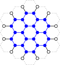
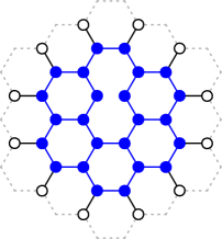
Figure 2: Left: Finite hexagonal lattice. The white vertices are considered to be the boundary vertices for the set of the blue (interior) vertices. Right: A finite hexagonal lattice with one blue edge removed. Theorems 1 and 2 show that the exact structure of such graphs can be uniquely recovered from the boundary spectral data.

         

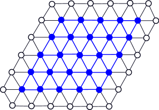
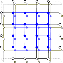
Figure 3: Left: Finite triangular lattice. The white vertices are the boundary vertices; the blue vertices are the interior vertices. Right: Finite two-level square ladder, made out of two layers of square lattices.

1.3 Examples

As primary examples, we consider several standard types of graphs satisfying the Two-Points Condition (Item 1 of 1).

Example 1.

All finite trees satisfy the Two-Points Condition, with the boundary vertices being all vertices of degree $1$.

This fact can be shown as follows. Recall that a tree is a connected graph containing no cycles. Take any subset $S$ of the interior vertices (i.e., vertices of degree at least $2$) of a tree with $|S|\geqslant 2$. If $|S|=2$, say $S=\{v_{1},v_{2}\}$, then both vertices in $S$ are extreme points. This can be argued as follows. Take the (unique) shortest path between $v_{1},v_{2}$, remove the edge incident to $v_{1}$ on this path, and one gets two disjoint subtrees. Consider the subtree containing $v_{1}$. One can see that any boundary vertex on this subtree realizes the extreme point condition for $v_{1}$. If $|S|>2$, pick two arbitrary points in $S$, say again $\{v_{1},v_{2}\}$, then in the same way, consider the subtree containing $v_{1}$ after removing the edge incident to $v_{1}$ on the shortest path between $v_{1},v_{2}$. If this subtree does not intersect with $S-\{v_{1}\}$, then any boundary vertex on this subtree realizes the extreme point condition for $v_{1}$. Otherwise if the subtree intersects with $S-\{v_{1}\}$ at another vertex $v^{\prime}_{1}\in S$, then consider further the subtree containing $v^{\prime}_{1}$ by the same construction. Repeat this procedure until one finds a subtree that only intersects with $S$ at one vertex, and the procedure stops in finite steps since the graph is finite. Repeating this procedure from $v_{2}$ gives another extreme point, which verifies the Two-Points Condition.

For general cyclic graphs (i.e., graphs containing at least one cycle), it is often not easy to see if the Two-Points Condition is satisfied. The following proposition shows a concrete way to test for the Two-Points Condition.

Proposition 1.8.

For a finite graph with boundary $(G,\partial G,E)$, the Two-Points Condition follows from the existence of a function $h:G\cup\partial G\to\mathbb{R}$ satisfying the following conditions:

1. the Lipschitz constant of $h$ is bounded by $1$, i.e. if $x\sim y$ then $|h(x)-h(y)|\leqslant 1$;

2. $|N_{\pm}(x)|=1$ for all $x\in G$, and $|N_{\pm}(z)|\leqslant 1$ for all $z\in\partial G$, where

   $$N_{+}(x)=\{y\in G\cup\partial G:\ y\sim x\,,\,h(y)=h(x)+1\},$$

   $$N_{-}(x)=\{y\in G\cup\partial G:\ y\sim x\,,\,h(y)=h(x)-1\}.$$

We call $N_{+}(x)$ the discrete gradient of $h$ at $x$, and $N_{-}(x)$ the discrete gradient of $-h$ at $x$.

Proof.

For any $S\subseteq G$ with $|S|\geqslant 2$, take the points where the function $h$ achieves maximum and minimum in $S$. Let $x_{0}\in S$ be any maximal point. By condition (2), we can take the unique path, denoted by $\gamma_{x_{0}}$, starting from $x_{0}$ such that each step increases the function $h$ by $1$. This path $\gamma_{x_{0}}$ can only pass each point of the graph at most once, and therefore the path must end somewhere since the whole graph is finite. Let $z_{0}$ be the point where the path $\gamma_{x_{0}}$ ends. By construction we know $|N_{+}(z_{0})|=0$, which indicates $z_{0}\in\partial G$ by condition (2). Observe that $h(z_{0})-h(x_{0})\geqslant d(x_{0},z_{0})$ as $\gamma_{x_{0}}$ may not be distance-minimizing.

We claim that $x_{0}$ is the unique nearest point in $S$ from $z_{0}$ (i.e. $x_{0}$ is an extreme point of $S$). Suppose not, and there exists another $x_{1}\in S,\,x_{1}\neq x_{0}$ such that $d(x_{1},z_{0})\leqslant d(x_{0},z_{0})$. Then condition (1) implies that

$$|h(x_{1})-h(z_{0})|\leqslant d(x_{1},z_{0})\leqslant d(x_{0},z_{0}).$$ (1.11)

We claim that the two equalities in (1.11) cannot hold at the same time. Suppose both equalities are achieved. We take the shortest path from $z_{0}$ to $x_{1}$, and then the length of this path is equal to $d(x_{0},z_{0})$ by the second equality. The function $h$ can only change $d(x_{0},z_{0})$ times along the shortest path from $z_{0}$ to $x_{1}$, and hence every change must be decreasing by $1$ in order to make both equalities hold. However, there can only exist one such path starting from $z_{0}$ due to condition (2), which is exactly the backward direction from $z_{0}$ to $x_{0}$. Along this path, $x_{0}$ would be reached in exactly $d(x_{0},z_{0})$ steps and hence $x_{1}=x_{0}$. Hence the equalities in (1.11) cannot hold at the same time, and we have $h(x_{1})>h(z_{0})-d(x_{0},z_{0})$. On the other hand, we already know $h(x_{0})\leqslant h(z_{0})-d(x_{0},z_{0})$ indicating $h(x_{1})>h(x_{0})$, which is a contradiction to the maximality of $x_{0}$. This shows $x_{0}$ is an extreme point of $S$.

The same argument shows that any minimal point is also an extreme point of $S$. Therefore the Two-Points Condition follows from the condition $|S|\geqslant 2$. ∎

Example 2.

Finite square, hexagonal (Figure 2, Left), triangular (Figure 3, Left), graphite and square ladder (Figure 3, Right) lattices satisfy the Two-Points Condition with the set of boundary vertices being the domain boundary.

We can apply Proposition 1.8 to verify this. For the square, hexagonal, graphite and square ladder lattices, the function $h$ can be chosen as the standard height function with respect to a proper floor. Note that for these lattices, it suffices to choose only the floor and the ceiling as the boundary. For triangular lattices, the function $h$ can be constructed as a group action, such that $h$ changes by $1/2$ along the horizontal direction and changes by $1$ along one of the other directions.

Example 3.

In the finite square, hexagonal, triangular, graphite and square ladder lattices, any horizontal edges can be removed and the obtained graphs still satisfy the Two-Points Condition. Here, the horizontal edges refer to the edges in the non-gradient directions with respect to the function $h$. See Figure 2 (Right). This is because removing such edges does not affect the conditions for the function $h$ in Proposition 1.8.

A finite square lattice with an interior vertex and all its edges removed also satisfies the Two-Points Condition. Essentially, one can repeat the proof of Proposition 1.8 to show this particular situation. However, it is necessary to choose all four sides as the boundary and use two different choices of the function $h$. (Intuitively speaking, removing one small square does not affect the ability to find maximal and minimal points in at least two directions.) More generally, removing one square of any size from a finite square lattice does not affect the Two-Points Condition.

Example 4.

Assume that a function $h:G\cup\partial G\to\mathbb{R}$ satisfies the conditions (1, 2) in Proposition 1.8 for a finite graph with boundary $(G,\partial G,E)$. Then one can add to the graph $(G,\partial G,E)$ additional edges $\{x,y\}$ that connect any two vertices $x,y\in G\cup\partial G$ satisfying $|h(x)-h(y)|<1$. Similarly, one can remove from the graph any edges $\{x,y\}$ that connect vertices $x,y\in G\cup\partial G$ satisfying $|h(x)-h(y)|<1$. The obtained graph and the function $h$ satisfy the conditions (1, 2) in Proposition 1.8, and hence the Two-Points Condition. This procedure can be used, for example, to add additional horizontal edges in the finite hexagonal lattice in Figure 2.

Example 5.

Graphs that satisfy the conditions given in Proposition 1.8 can be connected together so that these conditions stay valid. To do this, assume that real-valued functions $h_{1}$ and $h_{2}$, defined on disjoint finite graphs with boundary $(G_{1},\partial G_{1},E_{1})$ and $(G_{2},\partial G_{2},E_{2})$, satisfy the conditions (1, 2) in Proposition 1.8, respectively. Moreover, assume that there are $c\in\mathbb{R}$ and ordered sets $X_{1}=\{x_{1}^{1},x_{2}^{1},\dots,x_{k}^{1}\}\subseteq G_{1}\cup\partial G_{1}$ and $X_{2}=\{x_{1}^{2},x_{2}^{2},\dots,x_{k}^{2}\}\subseteq G_{2}\cup\partial G_{2}$, such that $|h_{2}(x^{2}_{j})+c-h_{1}(x^{1}_{j})|<1$ for all $j=1,2,\dots,k$. (In particular, such sets and $c$ always exist for $k=1$.) Then we consider $(G,\partial G,E)$ for $G=G_{1}\cup G_{2}$, $\partial G=\partial G_{1}\cup\partial G_{2}$ and $E=E_{1}\cup E_{2}\cup E_{12}$, where $E_{12}=\big{\{}\{x^{1}_{j},x^{2}_{j}\}:\ j=1,2,\dots,k\big{\}}$. We define a function $h$ on $G\cup\partial G$ by

$$h(x)=\begin{cases}h_{1}(x),&\hbox{for }x\in G_{1}\cup\partial G_{1},\\ h_{2}(x)+c,&\hbox{for }x\in G_{2}\cup\partial G_{2}.\end{cases}$$ (1.12)

Then this function $h$ satisfies the conditions (1, 2) in Proposition 1.8 for $(G,\partial G,E)$, and therefore the graph $(G,\partial G,E)$ satisfies the Two-Points Condition. Figure 3 is a special case of this example.

However, the Two-Points Condition does not hold (without declaring more boundary vertices) if one adds an additional vertex and connects it to any interior vertex with an additional edge. This is because the set of the two endpoints of that additional edge violates the Two-Points Condition. Let us also mention an example where the Two-Points Condition is not satisfied: the Kagome lattice.

This paper is organized as follows. We introduce relevant definitions and basic facts in Section 2. In Section 3, we define the discrete wave equation and study the wavefront propagation. Section 4 is devoted to proving our main results.

Acknowledgement. We thank the anonymous referee for thoroughly reading our paper and many valuable comments. H.I. was partially supported by Grant-in-Aid for Scientific Research (C) 20K03667 Japan Society for the promotion of Science. H.I. is indebted to JSPS. E.B., M.L. and J.L. were partially supported by Academy of Finland, grants 273979, 284715, 312110.

2.  Preliminaries

In this section, let $\mathbb{G}=(G,\partial G,E,\mu,g)$ be a finite weighted graph with boundary. First, we derive an elementary but important Green’s formula.

Lemma 2.1 (Green’s formula).

For two functions $u_{1},u_{2}:G\cup\partial G\to\mathbb{R}$, we have

$$\sum_{x\in G}\mu_{x}\big{(}u_{1}(x)\Delta_{G}u_{2}(x)-u_{2}(x)\Delta_{G}u_{1}(x)\big{)}=\sum_{z\in\partial G}\mu_{z}\big{(}u_{2}(z)\partial_{\nu}u_{1}(z)-u_{1}(z)\partial_{\nu}u_{2}(z)\big{)}.$$

Proof.

By definition (1.4),

$$\sum_{x\in G}\mu_{x}u_{1}(x)\Delta_{G}u_{2}(x) = \sum_{x\in G}\sum_{\begin{subarray}{c}y\sim x\\ y\in G\cup\partial G\end{subarray}}g_{xy}u_{1}(x)\big{(}u_{2}(y)-u_{2}(x)\big{)}$$

$$= \sum_{x\in G}\big{(}\sum_{y\sim x,y\in G}+\sum_{y\sim x,y\in\partial G}\big{)}g_{xy}u_{1}(x)\big{(}u_{2}(y)-u_{2}(x)\big{)}.$$

Observe that the indices and summations can be switched in the following way:

$$\sum_{x\in G}\sum_{y\sim x,y\in G}g_{xy}u_{1}(x)u_{2}(y)=\sum_{y\in G}\sum_{x\sim y,x\in G}g_{yx}u_{1}(y)u_{2}(x)=\sum_{x\sim y,x\in G}\sum_{y\in G}g_{yx}u_{1}(y)u_{2}(x).$$

Hence the summation over $x,y\in G$ cancels out, and we get

$$\sum_{x\in G}\mu_{x}\big{(}u_{1}(x)\Delta_{G}u_{2}(x)-u_{2}(x)\Delta_{G}u_{1}(x)\big{)}=\sum_{x\in G}\sum_{y\sim x,y\in\partial G}g_{xy}\big{(}u_{1}(x)u_{2}(y)-u_{2}(x)u_{1}(y)\big{)},$$

where we have used the fact that the weights are symmetric: $g_{xy}=g_{yx}$. Then the lemma follows from (1.5) and the following identity:

$$u_{1}(x)u_{2}(y)-u_{2}(x)u_{1}(y)=u_{2}(y)\big{(}u_{1}(x)-u_{1}(y)\big{)}+u_{1}(y)\big{(}u_{2}(y)-u_{2}(x)\big{)}.$$

∎

Next we consider the boundary distance functions and the closely related resolving sets of a graph, see [44, 64] and their generalizations in [43].

Definition 2.2.

Let $(G,\partial G,E)$ be a finite connected graph with boundary. We say $\partial G=\{z_{i}\}_{i=0}^{m-1}$ is a resolving set for $(G,\partial G,E)$, if the boundary distance coordinate

$$\big{(}d(\cdot,z_{0}),d(\cdot,z_{1}),\cdots,d(\cdot,z_{m-1})\big{)}:G\to\mathbb{R}^{m}$$

is injective, where $d$ denotes the distance on $(G\cup\partial G,E)$.

For any point $x\in G$, we denote by $r_{x}$ the boundary distance function

$$r_{x}:\partial G\to\mathbb{R},\qquad r_{x}(z)=d(x,z).$$ (2.1)

The set of boundary distance functions of a graph $\mathbb{G}$ is denoted by $\mathcal{R}(\mathbb{G})$. If $\partial G$ is a resolving set, the map $x\mapsto r_{x}$ from $G$ to $\mathcal{R}(\mathbb{G})$ is a bijection.

The minimal cardinality of resolving sets for a graph is called the metric dimension of the graph [44]. The boundary distance functions are extensively used in the study of inverse problems on manifolds, see e.g. [38, 47, 48, 57, 63].

The concept of resolving sets gives a rough idea on how to choose boundary points such that the inverse problem may be solvable. If the chosen boundary points do not form a resolving set, then there is little hope to solve the inverse problem from spectral data measured at those points.

Lemma 2.3.

The Two-Points Condition (Item 1 of 1) implies that $\partial G$ is a resolving set for $(G,\partial G,E)$.

Proof.

Suppose that $\partial G$ is not a resolving set for $(G,\partial G,E)$. Then by Definition 2.2, there exist two points $x_{1},x_{2}\in G$ such that $d(x_{1},z)=d(x_{2},z)$ for all $z\in\partial G$. However, the set $S=\{x_{1},x_{2}\}$ is a contradiction to the Two-Points Condition for $(G,\partial G,E)$. ∎

We point out that the Neumann spectral data for the equation (1.9) are not affected at all by edges between boundary points, since the Neumann boundary value (1.5) only counts edges from boundary points to interior points. In other words, the edges between boundary points are invisible to our Neumann spectral data. However, this limitation does not matter to us since the structure of the boundary is a priori given. What we will reconstruct in the next few sections is actually the reduced graph of $\mathbb{G}$, which is defined as follows.

Definition 2.4 (Reduced graph).

Let $\mathbb{G}=(G,\partial G,E,\mu,g)$ be a weighted graph with boundary. The reduced graph of $\mathbb{G}$ is defined as $\mathbb{G}_{re}=(G,\partial G,E_{re},\mu,g|_{E_{re}}),$ where

$$E_{re}=E-\big{\{}\{x,y\}\in E\,\big{|}\,x\in\partial G\text{ and }y\in\partial G\big{\}}.$$

A graph with boundary being strongly connected is equivalent to its reduced graph being connected. Note that $\mathbb{G}$ and $\mathbb{G}_{re}$ have identical Neumann spectral data due to the definition of the Neumann boundary value (1.5).

Reducing a graph affects distances as paths along edges between boundary points become forbidden. In the same way as Definition 1.2, the distance $d_{re}(x,y)$ on the reduced graph $(G\cup\partial G,E_{re})$ is defined through paths of $(G\cup\partial G,E_{re})$ from $x$ to $y$, instead of along paths of the original graph $(G\cup\partial G,E)$. Then clearly $d_{re}(x,y)\geqslant d(x,y)$ for any $x,y\in G\cup\partial G$. The change of distances also affects the $r$-neighbourhood $N_{re}(x,r)$ of $x\in G\cup\partial G$, which is defined by

$$N_{re}(x,r)=\big{\{}y\in G\cup\partial G\,\big{|}\,d_{re}(y,x)\leqslant r\big{\}}.$$

However, reducing a graph does not affect the Two-Points Condition.

Lemma 2.5.

If $x_{0}\in S$ is an extreme point of a subset $S\subseteq G$ realized by some $z\in\partial G$, then there exists $z_{0}\in\partial G$ also realizing the extreme point condition of $x_{0}$ such that none of the shortest paths from $x_{0}$ to $z_{0}$ pass through any other boundary point.

As a consequence, if $(G,\partial G,E)$ satisfies the Two-Points Condition (Item 1 of 1), then so does $(G,\partial G,E_{re})$ with respect to its distance function $d_{re}$.

Proof.

If any shortest path from $x_{0}$ to $z$ passes through another boundary point $z^{\prime}\in\partial G$, then $x_{0}$ is an extreme point also realized at $z^{\prime}$. Then we consider the set of all the boundary points with respect to which $x_{0}$ is an extreme point, and take a point $z_{0}$ (not necessarily unique) in this set with the minimal distance from $x_{0}$. It follows that $z_{0}$ is the desired boundary point; otherwise there is another boundary point in the set with a smaller distance from $x_{0}$.

Let $x_{0}\in S$ be an extreme point of $S$ with respect to $\partial G$ realized by $z_{0}\in\partial G$. By the argument above, we may assume that none of the shortest paths from $x_{0}$ to $z_{0}$ pass through any boundary point except for $z_{0}$. Reducing the graph will not affect this path or its length. On the other hand, no distances between points may decrease in the reduction. So this path is still the shortest path between $S$ and $z_{0}$ in the reduced graph. Hence $x_{0}$ is also an extreme point of $S$ with respect to $\partial G$ in the reduced graph. ∎

3.  Wave Equation

Definition 3.1 (Time derivatives).

For a function $u:G\times\mathbb{N}\to\mathbb{R}$, we define the discrete first and second time derivatives at $(x,t_{0})$ by

$$D_{t}u(x,t_{0})=u(x,t_{0}+1)-u(x,t_{0}),\qquad t_{0}\geqslant 0,$$

$$D_{tt}(x,t_{0})=u(x,t_{0}+1)-2u(x,t_{0})+u(x,t_{0}-1),\qquad t_{0}\geqslant 1.$$

These are sometimes called the forward difference and the second-order central difference in time.

We consider the following initial value problem for the discrete wave equation with the Neumann boundary condition:

$$\begin{cases}D_{tt}u(x,t)-\Delta_{G}u(x,t)+q(x)u(x,t)=0,&x\in G,\,t\geqslant 1,\\ \partial_{\nu}u(x,t)=0,&x\in\partial G,\,t\geqslant 0,\\ D_{t}u(x,0)=0,&x\in G,\\ u(x,0)=W(x),&x\in G\cup\partial G,\end{cases}$$ (3.1)

where the values of $u$ on $\partial G$ are uniquely determined by the values on $G$ via the Neumann boundary condition at each time step. More precisely, using the definition of the Neumann boundary value (1.5) gives

$$u(z)=\sum_{\begin{subarray}{c}x\sim z\\ x\in G\end{subarray}}g_{xz}u(x)\Big{/}\sum_{\begin{subarray}{c}x\sim z\\ x\in G\end{subarray}}g_{xz},\qquad z\in\partial G.$$ (3.2)

We require $\partial_{\nu}W|_{\partial G}=0$ for the compatibility of the initial value and Neumann boundary condition. The initial conditions and the boundary condition imply that $u(x,1)=u(x,0)=W(x)$ for all $x\in G\cup\partial G$.

Definition 3.2 (Waves).

Given $W:G\cup\partial G\to\mathbb{R}$ satisfying $\partial_{\nu}W|_{\partial G}=0$, denote by $u^{W}:(G\cup\partial G)\times\mathbb{N}\to\mathbb{R}$ the solution of the discrete wave equation (3.1) with the initial condition $u(\cdot,0)=W(\cdot)$ on $G\cup\partial G$. The function $W$ is called the initial value. In this paper, a wave refers to a solution of the wave equation (3.1).

Lemma 3.3.

Given any initial value $W:G\cup\partial G\to\mathbb{R}$ satisfying $\partial_{\nu}W|_{\partial G}=0$, the discrete wave equation (3.1) has a unique solution.

Proof.

The discrete wave equation is solved in the following way. The solution on $G\cup\partial G$ at times $t=0$ and $t=1$ are determined by the initial conditions. Afterwards, the value on $G$ at time $t\geqslant 2$ is calculated from the value on $(G\cup\partial G)\times\{t-1\}$ and on $G\times\{t-2\}$ by the equation $D_{tt}u-\Delta_{G}u+qu=0$. Then the formula (3.2) gives the value on $\partial G$ at time $t$. ∎

The main purpose of this section is to prove a wavefront lemma which will be used frequently in the next section. Item 2 of 1 is essential for the wavefront lemma, as the wave propagation may “speed up” due to the instantaneous effect of the boundary condition if a shortest path goes through the boundary. Under Item 2 of 1, distances of the reduced graph are realized by avoiding boundary points, which is essential to guarantee proper wave behaviour.

Lemma 3.4.

Let $\mathbb{G}$ be a finite connected graph with boundary satisfying Item 2 of 1. Suppose the reduced graph of $\mathbb{G}$ is connected. Let $x\in G$ and $z\in\partial G$. If $x\sim z$, then $d_{re}(x,p)\leqslant d_{re}(z,p)$ for any $p\in G\cup\partial G-\{z\}$.

Proof.

Let $x^{\prime}\in G$ be a point such that $x^{\prime}\sim z$ and $d_{re}(x^{\prime},p)=d_{re}(z,p)-1$. This point exists since distances are realised by paths in a connected graph. Such a point $x^{\prime}$ cannot be in $\partial G$, because there are no edges between boundary points in the reduced graph. We have $x,x^{\prime}\in G$ and $x\sim z$, $x^{\prime}\sim z$. Then by Item 2 of 1, we have $x\sim x^{\prime}$ if $x\neq x^{\prime}$. Hence the triangle inequality yields that $d_{re}(x,p)\leqslant d_{re}(x,x^{\prime})+d_{re}(x^{\prime},p)=d_{re}(z,p)$. If $x=x^{\prime}$, then $d_{re}(x,p)=d_{re}(z,p)-1<d_{re}(z,p)$. ∎

Recall that the Neumann boundary value (1.5) does not take into account the edges between boundary points. This means that waves cannot propagate from one boundary point to another without going through the interior. Hence the wavefront propagates by the distance function $d_{re}$ of the reduced graph, instead of the distance function of the original graph.

Lemma 3.5 (Wavefront).

Let $\mathbb{G}$ be a finite connected weighted graph with boundary satisfying Item 2 of 1. Suppose the reduced graph of $\mathbb{G}$ is connected. Let $x\in G,\,z\in\partial G$ and $t_{0}=d_{re}(x,z)$. Suppose $W:G\cup\partial G\to\mathbb{R}$ is an initial value satisfying $\partial_{\nu}W|_{\partial G}=0,\,W(z)=0$ and

$$\big{\{}y\in N_{re}(z,t_{0})\cap G\;\big{|}\;W(y)\neq 0\big{\}}\subseteq\{x\}.$$ (3.3)

Then the following properties hold for the wave $u^{W}$ generated by $W$:

1. If $W(x)>0$, then $t_{0}\geqslant 2$, $u^{W}(z,t_{0})>0$ and $u^{W}(z,t)=0$ for all $t<t_{0}$;

2. If $W(x)=0$, then $u^{W}(z,t)=0$ for all $t\leqslant t_{0}$.

Proof.

Let us prove the first claim of the lemma with $W(x)>0$. To start with, we show that $t_{0}=d_{re}(x,z)\geqslant 2$. Suppose $d_{re}(x,z)=1$. Let $x,y_{1},\ldots,y_{J}\in G$ be the interior points connected to $z\in\partial G$. The boundary conditions $W(z)=0$ and $\partial_{\nu}W(z)=0$ imply that

$$\sum_{\begin{subarray}{c}y\sim z\\ y\in G\end{subarray}}g_{yz}W(y)=0.$$

On the other hand, (3.3) implies that $W(y_{j})=0$ for $j=1,\ldots,J$. Hence the equation above reduces to $g_{xz}W(x)=0$, which is a contradiction as $g$ is defined to be positive. Hence $d_{re}(x,z)\geqslant 2$.

Let $z^{\prime}\in\partial G$, $z^{\prime}\neq z$. If $d_{re}(z^{\prime},z)\leqslant t_{0}-1$, then for any $x^{\prime}\in G$ with $x^{\prime}\sim z^{\prime}$, Lemma 3.4 implies that $d_{re}(x^{\prime},z)\leqslant d_{re}(z^{\prime},z)\leqslant t_{0}-1$, and hence $W(x^{\prime})=0$ by (3.3). Since this holds for all the interior points connected to $z^{\prime}$, the Neumann boundary condition yields that $W(z^{\prime})=0$. On the other hand, if $d_{re}(z^{\prime},z)=t_{0}$, then for any $x^{\prime}\in G$ with $x^{\prime}\sim z^{\prime}$, Lemma 3.4 implies that $d_{re}(x^{\prime},z)\leqslant t_{0}$, and hence $W(x^{\prime})\geqslant 0$. Note that $W(x^{\prime})$ may be nonzero in this case since possibly $x^{\prime}=x$. Then the Neumann boundary condition gives $W(z^{\prime})\geqslant 0$. Combining these observations, for any $p\in G\cup\partial G$, we have

$$W(p)\,\begin{cases}=0,&p\in G\cup\partial G,\,d_{re}(p,z)\leqslant t_{0}-1,\\ \geqslant 0,&p\in G\cup\partial G,\,d_{re}(p,z)=t_{0},\\ >0,&p=x.\end{cases}$$ (3.4)

By the initial conditions of the wave equation (3.1), $u^{W}(p,1)=u^{W}(p,0)=W(p)$ for all $p\in G\cup\partial G$. Hence (3.4) gives the wavefront behavior of the wave $u^{W}(\cdot,t)$ at time $t=0,1$.

To study the wavefront behavior of the wave $u^{W}(\cdot,t)$ at $t\geqslant 2$, it is convenient to use an induction formulation where (3.4) serves as the base case. The formulation is as follows: prove the following statement, by induction on $\tau=1,2,\ldots,t_{0}-1$, that for any $p\in G\cup\partial G$,

$$u^{W}(p,\tau)\,\begin{cases}=0,&p\in G\cup\partial G,\,d_{re}(p,z)\leqslant t_{0}-\tau,\\ \geqslant 0,&p\in G\cup\partial G,\,d_{re}(p,z)=t_{0}-\tau+1,\end{cases}$$ (3.5)

and that

$$u^{W}(x_{\tau},\tau)>0,$$ (3.6)

for some $x_{\tau}\in G$ satisfying $d_{re}(x_{\tau},z)=t_{0}-\tau+1$. For $\tau=1$, the claims (3.5) and (3.6) reduce to (3.4) by choosing $x_{\tau}=x$. This verifies the initial conditions for the induction. Assume that (3.5) and (3.6) hold for some $\tau\in\{1,2,\ldots,t_{0}-2\}$, we need to prove that (3.5) and (3.6) hold for $\tau+1$. We will spend most of the proof to argue this. Once (3.5) and (3.6) are proved, we will show in the end that the lemma can be proved from the $\tau=t_{0}-1$ case.

By the wave equation (3.1), we have

$$u^{W}(p,\tau+1)=2u^{W}(p,\tau)-u^{W}(p,\tau-1)+\Delta_{G}u^{W}(p,\tau)-q(p)u^{W}(p,\tau),$$ (3.7)

when $p\in G$ and $\tau\geqslant 1$. This formula and the Neumann boundary condition are what the induction is based on. First, we prove that (3.5) holds for $\tau+1$.

Let $p\in G$ satisfying $d_{re}(p,z)\leqslant t_{0}-(\tau+1)$. Then we see that the terms $2u^{W}(p,\tau),u^{W}(p,\tau-1)$ and $q(p)u^{W}(p,\tau)$ in (3.7) are all equal to zero by the induction assumption. Moreover, since $u^{W}(p,\tau)=0$, we have

$$\Delta_{G}u^{W}(p,\tau)=\frac{1}{\mu_{p}}\sum_{\begin{subarray}{c}y\sim p\\ y\in G\cup\partial G\end{subarray}}g_{py}u^{W}(y,\tau).$$

Let $y\in G\cup\partial G$ be any point connected to $p$. Then $d_{re}(y,z)\leqslant d_{re}(y,p)+d_{re}(p,z)\leqslant 1+t_{0}-(\tau+1)=t_{0}-\tau$, and hence $u^{W}(y,\tau)=0$ by the induction assumption. Thus (3.7) shows that $u^{W}(p,\tau+1)=0$ for all $p\in G$, $d_{re}(p,z)\leqslant t_{0}-(\tau+1)$.

On the other hand, if $p\in G$ satisfying $d_{re}(p,z)=t_{0}-(\tau+1)+1=t_{0}-\tau$, then for the same reason as above, we see that

$$u^{W}(p,\tau+1)=\Delta_{G}u^{W}(p,\tau)=\frac{1}{\mu_{p}}\sum_{\begin{subarray}{c}y\sim p\\ y\in G\cup\partial G\end{subarray}}g_{py}u^{W}(y,\tau).$$

If $y\in G\cup\partial G$ satisfies $y\sim p$, then $d_{re}(y,z)\leqslant d_{re}(y,p)+d_{re}(p,z)=1+t_{0}-\tau$, and hence $u^{W}(y,\tau)\geqslant 0$ by the induction assumption. Thus $u^{W}(p,\tau+1)\geqslant 0$. It remains to consider the case of $p\in\partial G$, and find $x_{\tau+1}$ for (3.6).

Let $p\in\partial G$. Instead of using (3.7) which is valid only in the interior, we can determine the sign of $u^{W}(p,\tau+1)$ by using the Neumann boundary condition $\partial_{\nu}u^{W}(p,\tau+1)=0$. Namely,

$$u^{W}(p,\tau+1)=\sum_{\begin{subarray}{c}y\sim p\\ y\in G\end{subarray}}g_{yp}u^{W}(y,\tau+1)\Big{/}{\sum_{\begin{subarray}{c}y\sim p\\ y\in G\end{subarray}}g_{yp}}.$$ (3.8)

Suppose $p\neq z$ and $d_{re}(p,z)\leqslant t_{0}-(\tau+1)$. Any interior point $y$ with $y\sim p$ satisfies that $d_{re}(y,z)\leqslant d_{re}(p,z)\leqslant t_{0}-(\tau+1)$ by Lemma 3.4. Since we have already showed that $u^{W}(y,\tau+1)=0$ for any $x\in G$ satisfying $d_{re}(y,z)\leqslant t_{0}-(\tau+1)$, it follows from (3.8) that $u^{W}(p,\tau+1)=0$. In the case of $p=z$, for any interior point $y$ adjacent to $z$ (i.e., $d_{re}(y,z)=1$), we have $u^{W}(y,\tau+1)=0$ if $d_{re}(y,z)=1\leqslant t_{0}-(\tau+1)$ is satisfied. This is applicable to all our induction steps since $\tau\leqslant t_{0}-2$, and therefore we have $u^{W}(z,\tau+1)=0$ due to (3.8).

For the second line in (3.5), let $p\in\partial G$ satisfying $d_{re}(p,z)=t_{0}-(\tau+1)+1=t_{0}-\tau$. In particular $p\neq z$ since $\tau<t_{0}$. As in the previous case, we see that any interior point $x$ with $x\sim p$ satisfies $d_{re}(x,z)\leqslant d_{re}(p,z)=t_{0}-\tau$. Since we have already showed that $u^{W}(x,\tau+1)\geqslant 0$ for such $x$, we get $u^{W}(p,\tau+1)\geqslant 0$. This concludes the proof of (3.5) by induction.

Next, we prove that (3.6) holds for $\tau+1$. The induction assumption gives that $u^{W}(p,\tau)\geqslant 0$ for any $p\in G\cup\partial G$ satisfying $d_{re}(p,z)=t_{0}-\tau+1$. Moreover, there exists one such $p\in G$, denoted by $x_{\tau}$, so that $u^{W}(x_{\tau},\tau)>0$. Let $\gamma$ be a shortest path of length $t_{0}-\tau+1$ from $x_{\tau}$ to $z$ in the reduced graph. Since $\tau\leqslant t_{0}-2$, this path is at least of length $3$. Let $x_{\tau+1}$ be the second vertex along this path, and then $d_{re}(x_{\tau+1},z)=t_{0}-\tau\geqslant 2$. Observe that $x_{\tau+1}$ is also an interior point: if not, then Lemma 3.4 implies that $d_{re}(x_{\tau},z)\leqslant d_{re}(x_{\tau+1},z)=t_{0}-\tau$ as $x_{\tau}\sim x_{\tau+1}$, contradiction.

To prove (3.6), it remains to prove that $u^{W}(x_{\tau+1},\tau+1)>0$. We consider the formula (3.7) with $p=x_{\tau+1}$. The induction assumption for (3.5) shows that $u^{W}(x_{\tau+1},\tau)$, $u^{W}(x_{\tau+1},\tau-1)$ and $q(x_{\tau+1})u^{W}(x_{\tau+1},\tau)$ are all equal to zero, since $d_{re}(x_{\tau+1},z)\leqslant t_{0}-\tau$. Thus by (3.7),

$$u^{W}(x_{\tau+1},\tau+1)=\Delta_{G}u^{W}(x_{\tau+1},\tau)=\frac{1}{\mu_{x_{\tau+1}}}\sum_{\begin{subarray}{c}y\sim x_{\tau+1}\\ y\in G\cup\partial G\end{subarray}}g_{yx_{\tau+1}}u^{W}(y,\tau).$$

For a point $y\in G\cup\partial G$ connected to $x_{\tau+1}$, we have $d_{re}(y,z)\leqslant t_{0}-\tau+1$, and therefore the induction assumption for (3.5) gives $u^{W}(y,\tau)\geqslant 0$. Notice that one of the points $y$ in the sum above is $x_{\tau}$, for which $u^{W}(x_{\tau},\tau)>0$. Hence the whole sum is positive. This concludes the proof of (3.6) by induction.

Now we turn to the statement of the lemma, with (3.5) and (3.6) in hand. We see that $u^{W}(z,t)=0$ for all $t<t_{0}$ by (3.5). At time $t_{0}$, the Neumann boundary condition gives

$$u^{W}(z,t_{0})=\sum_{\begin{subarray}{c}y\sim z\\ y\in G\end{subarray}}g_{yz}u^{W}(y,t_{0})\Big{/}{\sum_{\begin{subarray}{c}y\sim z\\ y\in G\end{subarray}}g_{yz}}.$$ (3.9)

Let $y\in G$ be an arbitrary point satisfying $y\sim z$. The formula (3.7) gives

$$u^{W}(y,t_{0})=2u^{W}(y,t_{0}-1)-u^{W}(y,t_{0}-2)+\Delta_{G}u^{W}(y,t_{0}-1)-q(y)u^{W}(y,t_{0}-1).$$

Since $u^{W}(y,t_{0}-1)=u^{W}(y,t_{0}-2)=0$ by (3.5), we have

$$\Delta_{G}u^{W}(y,t_{0}-1)=\frac{1}{\mu_{y}}\sum_{\begin{subarray}{c}p\sim y\\ p\in G\cup\partial G\end{subarray}}g_{yp}u^{W}(p,t_{0}-1).$$

Note that $d_{re}(p,z)\leqslant d_{re}(p,y)+d_{re}(y,z)=1+1=2$. If $d_{re}(p,z)=0$, then $p=z$ and $u^{W}(p,t_{0}-1)=u^{W}(z,t_{0}-1)=0$. If $d_{re}(p,z)=1$, then $u^{W}(p,t_{0}-1)=0$ by the first line of (3.5). If $d_{re}(p,z)=2$, then $u^{W}(p,t_{0}-1)\geqslant 0$ by the second line of (3.5). Hence from the equations above, we see that $\Delta_{G}u^{W}(y,t_{0}-1)\geqslant 0$ and consequently $u^{W}(y,t_{0})\geqslant 0$ for any $y\in G$ satisfying $y\sim z$. Furthermore, there exists a point $\hat{p}\in G$ with $d_{re}(\hat{p},z)=2$ such that $u^{W}(\hat{p},t_{0}-1)>0$ by (3.6). The condition $d_{re}(\hat{p},z)=2$ indicates that there exists a point $\hat{y}\in G$ such that $\hat{y}\sim z$ and $\hat{y}\sim\hat{p}$. Hence from the same equations above, we see that $\Delta_{G}u^{W}(\hat{y},t_{0}-1)>0$ and consequently $u^{W}(\hat{y},t_{0})>0$. Combining these with (3.9) yields that $u^{W}(z,t_{0})>0$.

The second claim of the lemma with $W(x)=0$ simply follows from the same proof as above but without the need for (3.6), and by replacing instances of $W\geqslant 0,W>0$ with $W=0$ and those of $u^{W}\geqslant 0,u^{W}>0$ with $u^{W}=0$. ∎

4.  The Inverse Spectral Problem

In this section, we reconstruct the graph structure and the potential from the Neumann boundary spectral data, and prove 1 and 2. Since the structure of the boundary is a priori given, it suffices to reconstruct the reduced graph $\mathbb{G}_{re}$ (recall Definition 2.4). The assumption that $\mathbb{G}$ is strongly connected is equivalent to $\mathbb{G}_{re}$ being connected. Due to Lemma 2.5 and the fact that removing edges between boundary points does not affect the boundary spectral data, without loss of generality, we assume $\mathbb{G}=\mathbb{G}_{re}$ throughout this section. In other words, we assume that there are no edges between boundary points in $\mathbb{G}$.

The full reconstruction process is divided into two main parts. The first part proves that under the Two-Points Condition, the Neumann boundary spectral data determine the Fourier coefficients of all $L^{2}$-normalized functions supported at one single interior point (and all boundary distance functions corresponding to interior points). The second part proves that these information then determines the graph structure and the weights.

4.1 Characterization by boundary data

In this subsection, we construct a characterization of the boundary distance functions by boundary data. We mention that the related constructions on partially ordered lattices that contain boundary distance functions as maximal elements have been used to study inverse problems on manifolds in [62].

Let $s:\partial G\to\mathbb{Z}_{+}$. We equip the set of such functions with the following partial order

$$\forall z\in\partial G:s_{1}(z)\leqslant s_{2}(z)\quad\Longrightarrow\quad s_{1}\leqslant s_{2}.$$ (4.1)

We consider the set of initial values for which the corresponding waves are not observed at the boundary before time $s(\cdot)$,

$$\mathcal{W}(s)=\{W:G\cup\partial G\to\mathbb{R}\;|\;\partial_{\nu}W|_{\partial G}=0,\,u^{W}(z,t)=0\textrm{ for all }z\in\partial G,\,t<s(z)\}.$$

Let $N=|G|$ be the number of interior vertices, and we define the set

$$\mathcal{U}=\{s:\partial G\to\mathbb{Z}_{+}\mid 2\leqslant s(\cdot)\leqslant N,\,\dim(\mathcal{W}(s))\neq 0\}.$$ (4.2)

We remark that given the Neumann boundary spectral data, the conditions of $\mathcal{W}(s)$ correspond to a system of linear equations on $\partial G$ for solving the Fourier coefficients of the initial value, which will be explained in details in the next subsection. As a consequence, the Neumann boundary spectral data determine the set $\mathcal{U}$.

Due to the linearity of the wave equation (3.1), the set $\mathcal{W}(s)$ is a linear space over $\mathbb{R}$, so $\dim(\mathcal{W}(s))$ is simply its dimension as a vector space. The condition $\dim(\mathcal{W}(s))\neq 0$ simply means that there exists a nonzero initial value such that the corresponding wave satisfies the conditions of $\mathcal{W}(s)$. Observe that the conditions of $\mathcal{W}(s)$ indicate that any initial value $W\in\mathcal{W}(s)$ vanishes on the whole boundary since $u^{W}(z,0)=W(z)$. Then the condition $u^{W}(z,t)=0$ for $t=0$ implies the same condition for $t=1$ due to the initial conditions of (3.1). Hence we only need to consider $s\geqslant 2$ in the definition above.

The set $\mathcal{U}$ is a set of functions equipped with the partial order (4.1). We are interested in its maximal elements with respect to the partial order, denoted by $\max(\mathcal{U})$.

Lemma 4.1.

Let $\mathbb{G}$ be a finite connected weighted graph with boundary satisfying 1. Then we have

$$\{r_{x}\mid x\in G-N(\partial G)\}\subseteq\max(\mathcal{U}).$$ (4.3)

Furthermore, for any nonzero initial value $W\in\mathcal{W}(r_{x})$ where $x\in G-N(\partial G)$, we have $\operatorname{supp}(W)=\{x\}$.

Proof.

For an arbitrary point $x\in G-N(\partial G)$, we first show that for any nonzero initial value $W\in\mathcal{W}(r_{x})$, we have $\operatorname{supp}(W)=\{x\}$ and consequently $r_{x}\in\mathcal{U}$ by Lemma 3.5. Observe that $r_{x}(\cdot)\geqslant 2$ due to $x\in G-N(\partial G)$, and $r_{x}(\cdot)\leqslant N$ since we assume no edges between boundary points and any shortest path between $x$ and a boundary point can pass at most $N-1$ interior points.

From the condition $W\in\mathcal{W}(r_{x})$, we see that the wave $u^{W}$ corresponding to this initial value satisfies $u^{W}(z,t)=0$ when $z\in\partial G$ and $t<r_{x}(z)$. Let

$$S=\{y\in G\mid W(y)\neq 0\}\cup\{x\}.$$

If $|S|\geqslant 2$, the Two-Points Condition in 1 implies that there exist $x_{0}\in S-\{x\}$ and $z_{0}\in\partial G$, such that $x_{0}$ is the unique nearest point in $S$ from $z_{0}$, which in particular yields $d(x_{0},z_{0})\leqslant d(x,z_{0})-1=r_{x}(z_{0})-1$. But by the propagation of the wavefront (Lemma 3.5), we see that $u^{W}(z_{0},t_{0})\neq 0$ for $t_{0}=d(x_{0},z_{0})$. This is a contradiction because $\mathcal{W}(r_{x})$ requires $u^{W}(z_{0},t_{0})=0$ for $t_{0}<r_{x}(z_{0})$. Therefore $|S|\leqslant 1$ and $\operatorname{supp}(W)\cap G\subseteq\{x\}$. Since $x\notin N(\partial G)$, we see by the Neumann boundary condition that $W=0$ on $\partial G$. Hence $\operatorname{supp}(W)=\{x\}$.

We next show that the boundary distance functions are maximal elements in $\mathcal{U}$. Let $x\in G-N(\partial G)$ and suppose there exists an element $s\in\mathcal{U}$ such that $s\geqslant r_{x}$. By definition of $\mathcal{U}$, there exists a nonzero initial value $W$ such that

$$u^{W}(z,t)=0,\qquad\forall z\in\partial G,\,t<s(z).$$ (4.4)

Since $r_{x}\leqslant s$, the same vanishing conditions hold for all $t<r_{x}(z)$. Then the same argument above yields $\operatorname{supp}(W)=\{x\}$. If $r_{x}(z^{\prime})<s(z^{\prime})$ for some boundary point $z^{\prime}\in\partial G$ then Lemma 3.5 shows that $u^{W}(z^{\prime},t^{\prime})\neq 0$ for $t^{\prime}=d(x,z^{\prime})=r_{x}(z^{\prime})$. This contradicts (4.4). Therefore if $r_{x}\leqslant s$, then $r_{x}=s$ and therefore $r_{x}$ is a maximal element in $\mathcal{U}$. ∎

Next, we recover the boundary distance functions corresponding to points in $G\cap N(\partial G)$. Let $s:\partial G\to\mathbb{Z}_{+}$, and we define

$$\mathcal{W}_{b}(s)=\{W:G\cup\partial G\to\mathbb{R}\mid\partial_{\nu}W|_{\partial G}=0,\,u^{W}(z,t)=0\textrm{ when }z\in\partial G,\,s(z)\geqslant 2$$

$$\textrm{and }t<s(z)\}$$ ,

and for $y\in G\cap N(\partial G)$, define the set

$$\mathcal{U}_{b}(y)=\{s:\partial G\to\mathbb{Z}_{+}\mid\dim(\mathcal{W}_{b}(s))\neq 0,\,s(\cdot)\leqslant N,\,s(z)=1\textrm{ only if }z\sim y\}.$$

Recall that $N=|G|$ is the number of interior points. Functions $s\in\mathcal{U}_{b}(y)$ can have $s(z)>1$ at $z\sim y$. As with the previous case, the set $\mathcal{U}_{b}(y)$ is also determined by the Neumann boundary spectral data, which will be explained in the next subsection.

One can show the following lemma by a similar argument as Lemma 4.1.

Lemma 4.2.

Let $\mathbb{G}$ be a finite connected weighted graph with boundary satisfying 1. Then for any $y\in G\cap N(\partial G)$, we have

$$r_{y}\in\max\big{(}\mathcal{U}_{b}(y)\big{)}.$$ (4.5)

Furthermore, for any nonzero initial value $W\in\mathcal{W}_{b}(r_{y})$ where $y\in G\cap N(\partial G)$, we have $supp(W)\cap G=\{y\}$.

Proof.

Following the argument in Lemma 4.1, for any nonzero initial value $W\in\mathcal{W}_{b}(r_{y})$, consider the set $S=\{x\in G\mid W(x)\neq 0\}\cup\{y\}$. If $|S|\geqslant 2$, we can find an extreme point $y_{0}\in G-\{y\}$ of $S$ with respect to some $z_{0}\in\partial G$. The extreme point condition implies that $z_{0}$ cannot be connected to $y$, and hence $W(z_{0})=u^{W}(z_{0},0)=0$ by the condition $W\in\mathcal{W}_{b}(r_{y})$. The assumptions of Lemma 3.5 are satisfied for $W$ and the pair of points $y_{0},z_{0}$, so $u^{W}(z_{0},t_{0})\neq 0$ for $t_{0}=d(y_{0},z_{0})$. But by the definition of the extreme point, we have $d(y_{0},z_{0})<d(y,z_{0})=r_{y}(z_{0})$. This contradicts the condition $u^{W}(z_{0},t)=0$ for $t<r_{y}(z_{0})$ of $W\in\mathcal{W}_{b}(r_{y})$, considering $z_{0}\not\sim y$. Hence $|S|=1$ and $\operatorname{supp}(W)\cap G=\{y\}$.

Let $y\in G\cap N(\partial G)$. We first show that $r_{y}\in\mathcal{U}_{b}(y)$. Clearly $r_{y}\leqslant N$ and $r_{y}(z)=1$ only at boundary points $z$ connected to $y$. It remains to show that there exists a nonzero initial value in $\mathcal{W}_{b}(r_{y})$. Consider an initial value $W$ satisfying $W(x)=1$ at $x=y$ and $W(x)=0$ otherwise in $G$. The values of $W$ on $\partial G$ are determined by the Neumann boundary condition (3.2). By the definition of $W_{b}(r_{y})$, it suffices to show that $u^{W}(z,t)=0$ for all $t<r_{y}(z)$ when $r_{y}(z)\geqslant 2$. At such boundary points $z$ satisfying $r_{y}(z)\geqslant 2$ (i.e. $z\not\sim y$), the Neumann condition gives $W(z)=0$. Moreover, we have $W=0$ at all points in $N(z,d(y,z))\cap G$ except for $y$ at which $W(y)>0$. Hence Lemma 3.5 yields that $u^{W}(z,t)=0$ for all $t<d(y,z)=r_{y}(z)$. Thus $r_{y}\in\mathcal{U}_{b}(y)$.

Next, we show that $r_{y}$ is maximal. Let $s\in\mathcal{U}_{b}(y)$ with $r_{y}\leqslant s$. By the definition of $\mathcal{U}_{b}(y)$, we have $s(\cdot)\leqslant N$ and $s(z)>1$ if $z\not\sim y$. Furthermore, there is a nonzero initial value $W\in\mathcal{W}_{b}(s)$ satisfying

$$u^{W}(z,t)=0,\qquad\forall z\in\partial G,\,s(z)\geqslant 2,\,t<s(z).$$ (4.6)

If $s(z)=1$ occurs, it follows from the definition of $\mathcal{U}_{b}(y)$ that $z\sim y$, i.e. $r_{y}(z)=1$. Since $r_{y}\leqslant s$, the wave $u^{W}$ satisfies the following possibly less strict set of conditions

$$u^{W}(z,t)=0,\qquad\forall z\in\partial G,\,r_{y}(z)\geqslant 2,\,t<r_{y}(z).$$

This exactly means $W\in\mathcal{W}_{b}(r_{y})$. Then the same argument above yields $\operatorname{supp}(W)\cap G=\{y\}$. Assume that $r_{y}(z^{\prime})<s(z^{\prime})$ for some $z^{\prime}\in\partial G$. This indicates that $s(z^{\prime})\geqslant 2$ as $r_{y}>0$. Hence (4.6) implies that $u^{W}(z^{\prime},t)=0$ for $t<s(z^{\prime})$, and in particular $W(z^{\prime})=u^{W}(z^{\prime},0)=0$. Then Lemma 3.5 shows that $u^{W}(z^{\prime},t^{\prime})\neq 0$ for $t^{\prime}=d(y,z^{\prime})<s(z^{\prime})$, which is a contradiction. Hence $r_{y}(z^{\prime})=s(z^{\prime})$ for all $z^{\prime}\in\partial G$, and therefore $r_{y}$ is maximal. ∎

To uniquely determine $G\cap N(\partial G)$, we need to find all maximal elements of $\mathcal{U}_{b}(y)$ for every $y\in G\cap N(\partial G)$. Then this set of maximal elements contains the set of boundary distance functions $\{r_{y}\}_{y\in G\cap N(\partial G)}$, which corresponds to the initial values supported only at one single point of $G\cap N(\partial G)$ in the interior. However in general, as with Lemma 4.1, there are more maximal elements than just the boundary distance functions.

To reconstruct the graph structure, we need to single out the actual boundary distance functions from the whole set of maximal elements. We will spend the rest of this subsection to address it.

Definition 4.3.

We define the arrival time of a wave with an initial value $W$ at a boundary point $z\in\partial G$, to be the earliest time $t\geqslant 1$ when $u^{W}(z,t)\neq 0$. Denote the arrival time at $z$ by $t^{W}_{z}$.

Definition 4.4.

Denote by $\mathcal{A}$ the set of all the $L^{2}(G)$-normalized initial values $W$ satisfying the following three conditions:

1. $W:G\cup\partial G\to\mathbb{R}$, $\partial_{\nu}W|_{\partial G}=0$, i.e. $W$ is an initial value;

2. $W\in\mathcal{W}(s)$ for some $s\in\max(\mathcal{U})$, or $W\in\mathcal{W}_{b}(s)$ for some $s\in\max(\mathcal{U}_{b}(y))$ and some $y\in G\cap N(\partial G)$, i.e. $W$ corresponds to a maximal element;

3. for all $z\in\partial G$, we have $u^{W}(z,t_{z}^{W})>0$, i.e. the first arrival of the wave at any boundary point is with a positive sign.

For $x\in G$, we use $W_{x}$ to denote a function satisfying $\partial_{\nu}W_{x}|_{\partial G}=0$, $\operatorname{supp}(W_{x})\cap G=\{x\}$ and $W_{x}(x)>0$. Finally, we define the set $\mathcal{A}_{0}$ as the $L^{2}$-normalized initial values supported at one single point,

$$\mathcal{A}_{0}=\left\{\frac{W_{x}}{\lVert W_{x}\rVert_{L^{2}(G)}}\,\middle|\,x\in G,\,\partial_{\nu}W_{x}|_{\partial G}=0,\,\operatorname{supp}(W_{x})\cap G=\{x\},\,W_{x}(x)>0\right\}.$$

Let us remark here regarding the motivation of Definition 4.4. In the next subsection, we will show in details that the Neumann boundary spectral data determine the sets $\mathcal{U}$ and $\mathcal{U}_{b}(y)$. This would imply that the Neumann boundary spectral data then determine the Fourier coefficients of functions in $\mathcal{A}$. The functions in $\mathcal{A}$ can be supported at multiple interior points, while what we really want are the functions in $\mathcal{A}_{0}$ supported at one single interior point. Therefore, we need to construct an algorithm (Lemma 4.8) to single out $\mathcal{A}_{0}$ from $\mathcal{A}$.

Lemma 4.5.

Let $\mathbb{G}$ be a finite connected weighted graph with boundary satisfying 1. Then $\mathcal{A}_{0}\subseteq\mathcal{A}$.

Proof.

Let $W\in\mathcal{A}_{0}$. Then $W$ is $L^{2}(G)$-normalized and it satisfies property 1 in Definition 4.4. Furthermore $W=W_{x}$ for some $x\in G$. We claim that $t_{z}^{W}=r_{x}(z)$ for all $z\in\partial G$.

This claim follows directly from the propagation of the wavefront (Lemma 3.5) if $x\in G-N(\partial G)$, which yields that $u^{W}(z,t_{z}^{W})>0$ for all $z\in\partial G$. If $x\in G\cap N(\partial G)$ we see that $t_{z}^{W}=r_{x}(z)$ when $r_{x}(z)\geqslant 2$ by Lemma 3.5. If $r_{x}(z)=1$, then $z\sim x$ and $u^{W}(z,t)$ is determined by the Neumann boundary condition (3.2), which gives $u^{W}(z,0)=u^{W}(z,1)>0$. Hence $t_{z}^{W}=1$ in this case by Definition 4.3. In conclusion, $t_{z}^{W}=r_{x}(z)$ and $u^{W}(z,t_{z}^{W})>0$ for all $z\in\partial G$, i.e. the property 3 of Definition 4.4. Moreover, Lemmas 4.1 and 4.2 imply that $t_{\cdot}^{W}$ is a maximal element, i.e. the property 2 with $s(z)=t_{z}^{W}$. ∎

Observe that $\mathcal{A}_{0}$ is an orthonormal basis of the linear span of $\mathcal{A}$ with respect to the $L^{2}(G)$-inner product.

Lemma 4.6.

Let $\mathbb{G}$ be a finite connected weighted graph with boundary satisfying Item 2 of 1.

1. Given any initial value $W$ satisfying $\partial_{\nu}W|_{\partial G}=0$ and the property 3 of Definition 4.4, if $x_{0}$ is an extreme point of $\operatorname{supp}(W)\cap G$, then $W(x_{0})>0$.

2. Given any nonzero initial value $W$ satisfying $\partial_{\nu}W|_{\partial G}=0$ and $W|_{G}\geqslant 0$, then for any $z\in\partial G$, we have

   $$t^{W}_{z}=\min_{x\in\operatorname{supp}(W)\cap G}t^{W_{x}}_{z}\,.$$

As a consequence, if $W,W_{0}$ are two nonnegative initial values satisfying the Neumann boundary condition and $\operatorname{supp}(W_{0})\cap G\subseteq\operatorname{supp}(W)\cap G$, then $t^{W_{0}}_{z}\geqslant t^{W}_{z}$ for any $z\in\partial G$.

Proof.

For the first claim, let $z_{0}\in\partial G$ be a boundary point realizing the extreme point condition of $x_{0}$. If $d(x_{0},z_{0})\geqslant 2$, the arrival time $t^{W}_{z_{0}}=d(x_{0},z_{0})$ due to Lemma 3.5. If $d(x_{0},z_{0})=1$, then $t^{W}_{z_{0}}=1$ due to the Neumann boundary condition for $W$. Hence the property 3, Lemma 3.5 and the Neumann boundary condition yield $W(x_{0})>0$.

Next, consider the second claim. Due to $W|_{G}\geqslant 0$, the initial value $W$ restricted to $G$ can be written as

$$W|_{G}=\sum_{x\in\operatorname{supp}(W)\cap G}{\alpha}_{x}W_{x}|_{G}$$

for some positive numbers $\alpha_{x}$, where $W_{x}(x)=1$ and $W_{x}(y)=0$ if $y\in G-\{x\}$. Since $W$ and each $W_{x}$ determine their boundary values uniquely and linearly from their values on $G$ by (3.2), the form above extends to the whole graph $G\cup\partial G$. By linearity and the uniqueness of the solution of (3.1), the wave $u^{W}$ has the following form at any $z\in\partial G$ and $t\in\mathbb{N}$,

$$u^{W}(z,t)=\sum_{x\in\operatorname{supp}(W)\cap G}\alpha_{x}u^{W_{x}}(z,t).$$

Since $u^{W_{x}}(z,t^{W_{x}}_{z})>0$ for any $z\in\partial G$ by Lemma 3.5 and all $\alpha_{x}$ are positive, we know that the earliest time $u^{W}(z,\cdot)$ becomes nonzero is the earliest time when any of $u^{W_{x}}(z,\cdot)$ becomes nonzero. This shows that for any $z\in\partial G$,

$$t^{W}_{z}=\min_{x\in\operatorname{supp}(W)\cap G}t^{W_{x}}_{z}.$$

The last part of the lemma follows from the condition that $\operatorname{supp}(W_{0})\cap G\subseteq\operatorname{supp}(W)\cap G$, since a minimum over a smaller set can only be larger. ∎

Lemma 4.7.

Let $\mathbb{G}$ be a finite connected weighted graph with boundary satisfying 1. If an initial value $W$ satisfies $W|_{G}\geqslant 0$ and $|\operatorname{supp}(W)\cap G|\geqslant 2$, then $W\notin\mathcal{A}$.

Proof.

Denote $S=\{x\in G\mid W(x)\neq 0\}$ and we have $|S|\geqslant 2$ by assumption. We will show that the maximality requirement (2) of Definition 4.4 fails if (1) is satisfied.

First, let us bring forth a contradiction from the assumption that $W\in\mathcal{W}(s)$ for some $s\in\max(\mathcal{U})$. By the Two-Points Condition, there exists $x_{1}\in S$ and $z_{1}\in\partial G$, such that $x_{1}$ is the unique nearest point in $S$ from $z_{1}$. Since $W\in\mathcal{W}(s)$ and $s(z_{1})\geqslant 2$ as $s\in\mathcal{U}$, we have $W(z_{1})=u^{W}(z_{1},0)=0$. Then Lemma 3.5 implies that $t^{W}_{z_{1}}=d(x_{1},z_{1})$ and $2\leqslant s(z_{1})\leqslant t^{W}_{z_{1}}$. We consider the following modified function $s^{\prime}:\partial G\to\mathbb{Z}_{+}$ defined by $s^{\prime}(z_{1})=s(z_{1})+1$ and equal to $s$ at all other boundary points.

Now we prove that $s^{\prime}\in\mathcal{U}$ and consequently $s$ cannot be maximal in $\mathcal{U}$. On one hand, we have $s^{\prime}\geqslant s\geqslant 2$. On the other hand, we have $s^{\prime}\leqslant N$. This is because if $s(z_{1})=N$ then $d(x_{1},z_{1})\geqslant N$, which means that all $y\in S-\{x_{1}\}$ are at least distance $N+1$ from $z_{1}$. But this is impossible since there are only $N$ interior points, considering that distances (precisely $d_{re}$ on the reduced graph $\mathbb{G}_{re}$) are realized by paths passing through interior points by Lemma 3.4. Hence $2\leqslant s^{\prime}\leqslant N$ and it remains to show that $\mathcal{W}(s^{\prime})$ is nontrivial. Define another initial value $W_{0}$ to be $W_{0}(x_{1})=0$ and equal to $W$ elsewhere on $G$. By the propagation of the wavefront (Lemma 3.5), we have $u^{W_{0}}(z_{1},t)=0$ for $t\leqslant d(x_{1},z_{1})$. Since $s(z_{1})\leqslant t^{W}_{z_{1}}=d(x_{1},z_{1})$ and $s^{\prime}(z_{1})=s(z_{1})+1$, we have $u^{W_{0}}(z_{1},t)=0$ for $t<s^{\prime}(z_{1})$. Since $W|_{G}\geqslant 0$, the arrival time of the wave $u^{W_{0}}$ at any other boundary point is no earlier than that of $u^{W}$ by Lemma 4.6. This shows $W_{0}\in\mathcal{W}(s^{\prime})$ and it is a nontrivial element since $|S|\geqslant 2$. Hence $s^{\prime}\in\mathcal{U}$ and $s$ cannot be maximal.

Next we consider $W\in\mathcal{W}_{b}(s_{b})$ for some $s_{b}\in\mathcal{U}_{b}(y)$ and show that $s_{b}$ cannot be maximal. Following the previous argument, we can find $x_{1}\in S$ and $z_{1}\in\partial G$, such that $x_{1}$ is the unique nearest point in $S$ from $z_{1}$. If $s_{b}(z_{1})\geqslant 2$, then the previous argument applies. Otherwise if $s_{b}(z_{1})=1$, then $z_{1}\sim y$. We define $s_{b}^{\prime}:\partial G\to\mathbb{Z}_{+}$ by $s_{b}^{\prime}(z_{1})=2$ and equal to $s_{b}$ at all other boundary points. As before, we see that $s_{b}^{\prime}\leqslant N$, and $s_{b}^{\prime}(z)=1$ implies $z\sim y$. It remains to show that there is a nontrivial initial value $W_{0}\in\mathcal{W}_{b}(s_{b}^{\prime})$. We choose $W_{0}(x_{1})=0$ and equal to $W$ elsewhere on $G$. Since $x_{1}$ is an extreme point of $S$ with respect to $z_{1}$ and $W_{0}(x_{1})=0$, we have $W_{0}(z_{1})=0$ by the Neumann boundary condition. This implies that $u^{W_{0}}(z_{1},0)=u^{W_{0}}(z_{1},1)=W_{0}(z_{1})=0$, and hence $u^{W_{0}}(z_{1},t)=0$ for $t<s_{b}^{\prime}(z_{1})$. Then the same argument as for the earlier case shows that $u^{W_{0}}(z,t)=0$ for $t<s_{b}^{\prime}(z)$ when $s_{b}^{\prime}(z)\geqslant 2$. Thus we find a nontrivial initial value $W_{0}\in\mathcal{W}_{b}(s_{b}^{\prime})$. Therefore $s_{b}$ cannot be maximal in $\mathcal{U}_{b}(y)$. ∎

Finally, we use the following criteria to distinguish $\mathcal{A}_{0}$ from $\mathcal{A}$.

Lemma 4.8.

Let $\mathbb{G}$ be a finite connected weighted graph with boundary satisfying 1. Then a subset $\tilde{\mathcal{A}}\subseteq\mathcal{A}$ satisfies the following two properties

1. $\tilde{\mathcal{A}}$ is an orthogonal basis of the linear span of $\mathcal{A}$ in $L^{2}(G)$;

2. for any $W\in\mathcal{A}-\tilde{\mathcal{A}}$, there exists $\tilde{W}\in\tilde{\mathcal{A}}$ such that $\langle W,\tilde{W}\rangle_{L^{2}(G)}<0$,

if and only if $\tilde{\mathcal{A}}=\mathcal{A}_{0}$.

Remark.

Elements of $\mathcal{A}$ are normalized, so we are actually searching for an orthonormal basis satisfying Property (2). Property (1) can also be formulated as follows: $\tilde{\mathcal{A}}$ has cardinality equal to $|G|$, and its elements are mutually orthogonal with respect to the $L^{2}(G)$-inner product.

Proof.

First, we show that $\mathcal{A}_{0}$ satisfies these two properties. The set $\mathcal{A}_{0}$ satisfies Property (1) as a direct consequence of Lemma 4.5. Since every function in $\mathcal{A}-\mathcal{A}_{0}$ is supported at multiple interior points by the definition of $\mathcal{A}_{0}$, Lemma 4.7 implies that any function $W\in\mathcal{A}-\mathcal{A}_{0}$ must have a negative value at some interior point, say at $x\in G$. Then the condition $\langle W,\tilde{W}\rangle_{L^{2}(G)}<0$ is satisfied with $\tilde{W}=W_{x}$. Hence Property 2 is satisfied for $\mathcal{A}_{0}$.

Next, we prove the “only if” direction. We claim that if $\tilde{\mathcal{A}}\nsubseteq\mathcal{A}_{0}$, then the Properties (1) and (2) cannot be satisfied at the same time. Suppose $\tilde{\mathcal{A}}\nsubseteq\mathcal{A}_{0}$ and Property (1) is true. The set $\tilde{\mathcal{A}}$ consists of two types of initial values: a) initial values supported at one single point in the interior (corresponding to the boundary distance functions), and b) initial values supported at multiple points in the interior (where interactions occur). Note that $\tilde{\mathcal{A}}$ may not contain the former type of initial values, but it must contain the latter type of initial values since $\tilde{\mathcal{A}}-\mathcal{A}_{0}\neq\emptyset$ by assumption. Property (1) implies that the support of these two types of initial values does not intersect.

Consider the union of the support (intersected with $G$) of all the initial values of type b) in $\tilde{\mathcal{A}}$, denoted by

$$S=\bigcup_{{W\in\tilde{\mathcal{A}},\ W\textrm{ of type b)}}}\operatorname{supp}(W)\cap G.$$

By the Two-Points Condition, we can find an extreme point $\tilde{x}\in G$ of $S$. Then we consider the $L^{2}(G)$-normalized initial value $W_{\tilde{x}}\in\mathcal{A}$ supported at $\tilde{x}\in G$ with $W_{\tilde{x}}(\tilde{x})>0$. Orthogonality implies that $W_{\tilde{x}}\notin\tilde{\mathcal{A}}$, or equivalently $W_{\tilde{x}}\in\mathcal{A}-\tilde{\mathcal{A}}$. For any $\tilde{W}\in\tilde{\mathcal{A}}$ with $\langle W_{\tilde{x}},\tilde{W}\rangle_{L^{2}(G)}\neq 0$, we know that $\tilde{W}$ is supported at multiple points containing $\tilde{x}$. The condition that $\tilde{x}$ is an extreme point of $S$ implies that $\tilde{x}$ is also an extreme point of its subset $\operatorname{supp}(\tilde{W})\cap G$. Then $\tilde{W}(\tilde{x})>0$ by Lemma 4.6(1). As a result, the positivity implies

$$\langle W_{\tilde{x}},\tilde{W}\rangle_{L^{2}(G)}=\mu_{\tilde{x}}W_{\tilde{x}}(\tilde{x})\tilde{W}(\tilde{x})>0.$$

Hence $\langle W_{\tilde{x}},\tilde{W}\rangle_{L^{2}(G)}\geqslant 0$ for all $\tilde{W}\in\tilde{\mathcal{A}}$. This contradicts Property (2), and therefore proves the claim.

The claim shows that $\tilde{\mathcal{A}}\subseteq\mathcal{A}_{0}$ for any subset $\tilde{\mathcal{A}}\subseteq\mathcal{A}$ satisfying both properties. The set $\mathcal{A}_{0}$ is an orthogonal basis of the linear span of $\mathcal{A}$, and the only subset of $\mathcal{A}_{0}$ also forming a basis is $\mathcal{A}_{0}$ itself. Hence Property (1) yields $\tilde{\mathcal{A}}=\mathcal{A}_{0}$. ∎

4.2 Determination from spectral data

In this subsection, we will tie in the previous subsection’s objects to the spectral and boundary data of a graph. We will show that if two graphs have the same a priori data, then the spectral characterization of various objects, such as $\mathcal{U}$, $\mathcal{A}_{0}$ from the previous subsection, of these two graphs coincide. This leads to the conclusion that the inverse spectral problem is solvable.

Without loss of generality, we still assume $\mathbb{G}=\mathbb{G}_{re}$ throughout this section.

Lemma 4.9.

Let $\mathbb{G}$ be a finite connected weighted graph with boundary, and $q$ be a real-valued potential function on $G$. Let $\{\phi_{j}\}_{j=1}^{N}$ be the orthonormalized Neumann eigenfunctions of $(\mathbb{G},q)$. For any function $W:G\cup\partial G\to\mathbb{R}$, denote

$$\widehat{W}(j)=\langle W,\phi_{j}\rangle_{L^{2}(G)},\quad\widehat{W}=\big{(}\widehat{W}(1),\cdots,\widehat{W}(N)\big{)}\in\mathbb{R}^{N}.$$

If $W$ is an initial value for (3.1), i.e. satisfying $\partial_{\nu}W|_{\partial G}=0$, we have

$$W(x)=\sum_{j=1}^{N}\widehat{W}(j)\phi_{j}(x),\quad\forall\,x\in G\cup\partial G.$$

Conversely, given any $(c_{j})_{j=1}^{N}\in\mathbb{R}^{N}$, $\sum_{j}c_{j}\phi_{j}$ gives an initial value for (3.1).

Proof.

Since $\mathbb{G}$ is connected and there are no edges between boundary points by assumption, every boundary point is connected to the interior. Then the claims are a direct consequence of the orthonormality of the eigenfunctions in $L^{2}(G)$, (3.2) and $\partial_{\nu}\phi_{j}|_{\partial G}=0$. ∎

Notation.

Given a complete orthonormal family of Neumann eigenfunctions of $(\mathbb{G},q)$ and $V\subseteq L^{2}(G)$, we denote $\widehat{V}=\{\widehat{f}\in\mathbb{R}^{N}\mid f\in V\}.$ If $\mathbb{G}^{\prime}$ is another finite weighted graph with boundary, then we denote by $V^{\prime}$ a subset of $L^{2}(G^{\prime})$. In this case, $\widehat{V^{\prime}}$ is defined the same as above, but the hat-notation itself is defined using the eigenfunctions $\phi_{j}^{\prime}$ of $\mathbb{G}^{\prime}$ rather than those of $\mathbb{G}$.

The following lemma enables us to calculate a wave at any boundary point and any time, if we know the Neumann boundary spectral data and the Fourier transform (or the spectral representation) of the initial value of the wave.

Lemma 4.10.

Let $\mathbb{G}$ be a finite connected weighted graph with boundary, and $q$ be a real-valued potential function on $G$. Let $(\lambda_{j},\phi_{j})_{j=1}^{N}$ be the Neumann eigenvalues and orthonormalized Neumann eigenfunctions of $(\mathbb{G},q)$. Suppose $W$ is the initial value of some wave $u^{W}$ satisfying the wave equation (3.1). Then

$$u^{W}(x,t) =\sum_{\{j\mid\lambda_{j}=0\}}\widehat{W}(j)\phi_{j}(x)+\sum_{\{j\mid\lambda_{j}=4\}}\widehat{W}(j)(-2t+1)(-1)^{t}\phi_{j}(x)$$

$$\phantom{=}+\sum_{\{j\mid\lambda_{j}\notin\{0,4\}\}}\widehat{W}(j)\frac{\beta_{j,1}^{t}-\beta_{j,2}^{t}-(\beta_{j,1}^{t-1}-\beta_{j,2}^{t-1})}{\beta_{j,1}-\beta_{j,2}}\phi_{j}(x)\,,$$

where

$$\beta_{j,1}=-\frac{\lambda_{j}}{2}+1-\sqrt{\left(\frac{\lambda_{j}}{2}-1\right)^{2}-1}\;,\quad\beta_{j,2}=-\frac{\lambda_{j}}{2}+1+\sqrt{\left(\frac{\lambda_{j}}{2}-1\right)^{2}-1}\;.$$ (4.7)

Conversely, given any $\widehat{W}\in\mathbb{R}^{N}$, then the wave $u^{W}$ defined as above solves (3.1) with the initial value $W=\sum_{j=1}^{N}\widehat{W}(j)\phi_{j}$.

Proof.

By assumption, every boundary point is connected to the interior. The wave satisfies $\partial_{\nu}u^{W}|_{\partial G\times\mathbb{N}}=0$, so the orthonormality of $\{\phi_{j}\}_{j=1}^{N}$ in $L^{2}(G)$ and (3.2) imply that

$$u(x,t)=\sum_{j=1}^{N}a_{j}(t)\phi_{j}(x)$$

on $(G\cup\partial G)\times\mathbb{N}$ for some functions $a_{j}:\mathbb{N}\to\mathbb{R}$. The wave equation (3.1) and the eigenvalue problem (1.10) yield that

$$a_{j}(t+1)+(\lambda_{j}-2)a_{j}(t)+a_{j}(t-1)=0$$ (4.8)

for all $t\in\mathbb{Z}_{+}$. The solutions to the associated characteristic equation $\beta_{j}^{2}+(\lambda_{j}-2)\beta_{j}+1=0$ are shown in the lemma statement. The characteristic equation has two identical solutions if $\lambda_{j}=0$ or $4$, in which case the solutions are $1$ or $-1$. Hence $a_{j}$ has the following form:

$$a_{j}(t)=\begin{cases}b_{j}t+c_{j},&\lambda_{j}=0,\\ (b_{j}t+c_{j})(-1)^{t},&\lambda_{j}=4,\\ b_{j}\beta_{j,1}^{t}+c_{j}\beta_{j,2}^{t},&\lambda_{j}\notin\{0,4\},\end{cases}\qquad t\in\mathbb{N}.$$ (4.9)

Recall that $u^{W}(\cdot,0)=u^{W}(\cdot,1)$. Then the formula for $a_{j}$ implies that

$$\sum_{\{j\mid\lambda_{j}=0\}}c_{j}\phi_{j}+\sum_{\{j\mid\lambda_{j}=4\}}c_{j}\phi_{j}+\sum_{\{j\mid\lambda_{j}\notin\{0,4\}\}}(b_{j}+c_{j})\phi_{j}$$

$$=\sum_{\{j\mid\lambda_{j}=0\}}(b_{j}+c_{j})\phi_{j}-\sum_{\{j\mid\lambda_{j}=4\}}(b_{j}+c_{j})\phi_{j}+\sum_{\{j\mid\lambda_{j}\notin\{0,4\}\}}(b_{j}\beta_{j,1}+c_{j}\beta_{j,2})\phi_{j}.$$

Taking the inner product with any $\phi_{j}$, and the orthonormality of $\phi_{j}$ allows us to solve $b_{j}$ as a function of $c_{j},\beta_{j,1}$ and $\beta_{j,2}$ for each $j=1,\ldots,N$. This gives

$$b_{j}=\begin{cases}0,&\lambda_{j}=0,\\ -2c_{j},&\lambda_{j}=4,\\ -c_{j}\frac{\beta_{j,2}-1}{\beta_{j,1}-1},&\lambda_{j}\notin\{0,4\}.\end{cases}$$

Note that $\beta_{j,1},\beta_{j,2}\neq\pm 1$ if $\lambda_{j}\notin\{0,4\}$. Hence we obtain the formula for the wave:

$$u^{W}(x,t) =\sum_{\{j\mid\lambda_{j}=0\}}c_{j}\phi_{j}(x)+\sum_{\{j\mid\lambda_{j}=4\}}c_{j}(-2t+1)(-1)^{t}\phi_{j}(x)+$$

$$\phantom{=}+\sum_{\{j\mid\lambda_{j}\notin\{0,4\}\}}c_{j}\left(-\frac{\beta_{j,2}-1}{\beta_{j,1}-1}\beta_{j,1}^{t}+\beta_{j,2}^{t}\right)\phi_{j}(x)\,,$$

for $x\in G\cup\partial G$ and $t\in\mathbb{N}$. This satisfies the second initial condition, the Neumann boundary condition and the wave equation in (3.1). By Lemma 4.9, the first initial condition $u^{W}(x,0)=W(x)$ gives that

$$c_{j}=\begin{cases}\widehat{W}(j),&\lambda_{j}=0,\\ \widehat{W}(j),&\lambda_{j}=4,\\ \widehat{W}(j)\frac{\beta_{j,1}-1}{\beta_{j,1}-\beta_{j,2}},&\lambda_{j}\notin\{0,4\}.\end{cases}$$

The first claim of the lemma follows after plugging these into the formula for the wave. The converse claim is a straightforward calculation whose details are actually scattered in the proof of the first claim. ∎

In our setting, we are working with two graphs having the same boundary and the same Neumann boundary spectral data. For convenience, we make use of the following pullback notation.

Notation.

Given two finite weighted graphs with boundary $\mathbb{G},\mathbb{G}^{\prime}$ and a boundary-isomorphism $\Phi_{0}$ (Definition 1.6), we define the following notation.

• For $f^{\prime}:\partial G^{\prime}\to\mathbb{R}$, we denote $\Phi_{0}^{\ast}f^{\prime}=f^{\prime}\circ(\Phi_{0}|_{\partial G})$.

• If $S^{\prime}$ is a set of functions on $\partial G^{\prime}$, denote $\Phi_{0}^{\ast}S^{\prime}=\{\Phi_{0}^{\ast}f^{\prime}\mid f^{\prime}\in S^{\prime}\}$.

This notation defines $\Phi_{0}^{\ast}f^{\prime}:\partial G\to\mathbb{R}$, and $\Phi_{0}^{\ast}S^{\prime}$ as a set of functions on $\partial G$.

We consider initial values not just as functions on the graph, but also as abstract points in $\mathbb{R}^{N}$ using their Fourier series representation in Lemma 4.9. Lemma 4.10 shows that the spectral (Fourier) coefficients of an initial value $W$ uniquely determine the boundary values of the corresponding wave $u^{W}$.

Lemma 4.11.

Let $\mathbb{G},\mathbb{G}^{\prime}$ be two finite connected weighted graphs with boundary, and $q,q^{\prime}$ be real-valued potential functions on $G,G^{\prime}$. Suppose $(\mathbb{G},q)$ is spectrally isomorphic to $(\mathbb{G}^{\prime},q^{\prime})$ with a boundary-isomorphism $\Phi_{0}$, namely

$$(\lambda_{j},\phi_{j}|_{\partial G})_{j=1}^{N}=(\lambda_{j}^{\prime},\Phi_{0}^{\ast}(\phi_{j}|_{\partial G^{\prime}}))_{j=1}^{N}.$$

Let $(c_{j})_{j=1}^{N}\in\mathbb{R}^{N}$, $W=\sum_{j=1}^{N}c_{j}\phi_{j},$ $W^{\prime}=\sum_{j=1}^{N}c_{j}\phi_{j}^{\prime},$ and $u^{W},u^{W^{\prime}}$ be the corresponding solution to the wave equation (3.1) in $\mathbb{G},\mathbb{G}^{\prime}$. Then $u^{W}(z,t)=u^{W^{\prime}}(\Phi_{0}(z),t)$ for all $z\in\partial G$ and $t\in\mathbb{N}$.

Proof.

This is a direct consequence of the representation formula for $u^{W},u^{W^{\prime}}$ in Lemma 4.10, since $\widehat{W}(j)=c_{j}=\widehat{W^{\prime}}(j)$, $\lambda_{j}=\lambda_{j}^{\prime}$ and $\phi_{j}=\phi_{j}^{\prime}\circ\Phi_{0}$ on $\partial G$. ∎

We remark that a full boundary-isomorphism is not needed for this lemma; a simple bijection $\partial G\to\partial G^{\prime}$ which makes the boundary spectral data equivalent is enough.

Our next few tasks are to show that various objects from Section 4.1 are equivalent, or that their spectral representations are the same for two spectrally isomorphic graphs. Recall the definitions of the various objects $\mathcal{W},\mathcal{W}_{b},\mathcal{U},\mathcal{U}_{b}$ which were defined just before Lemmas 4.1 and 4.2. The following lemma shows that knowing the Neumann boundary spectral data leads to the knowledge of the sets $\mathcal{U},\mathcal{U}_{b}$.

Lemma 4.12.

Let $\mathbb{G},\mathbb{G}^{\prime}$ be two finite connected weighted graphs with boundary, and $q,q^{\prime}$ be real-valued potential functions on $G,G^{\prime}$. Suppose $(\mathbb{G},q)$ is spectrally isomorphic to $(\mathbb{G}^{\prime},q^{\prime})$ with a boundary-isomorphism $\Phi_{0}$. Then $\widehat{\mathcal{W}}(s)=\widehat{\mathcal{W}^{\prime}}(s^{\prime})$ and $\widehat{\mathcal{W}_{b}}(s)=\widehat{\mathcal{W}_{b}^{\prime}}(s^{\prime})$ for all $s:\partial G\to\mathbb{Z}_{+}$ and $s^{\prime}=s\circ(\Phi_{0}|_{\partial G})^{-1}$. As a consequence,

$$\mathcal{U}=\Phi_{0}^{\ast}\mathcal{U}^{\prime},\qquad\mathcal{U}_{b}(y)=\Phi_{0}^{\ast}\big{(}\mathcal{U}_{b}^{\prime}(y^{\prime})\big{)},$$

for all $y\in G\cap N(\partial G)$ and $y^{\prime}=\Phi_{0}(y)$.

Proof.

We use the notation $s^{\prime}=s\circ(\Phi_{0}|_{\partial G})^{-1}$ throughout this proof. By symmetry, it suffices to prove that $\widehat{\mathcal{W}}(s)\subseteq\widehat{\mathcal{W}^{\prime}}(s^{\prime})$. Suppose $\widehat{W}=(c_{j})_{j=1}^{N}\in\mathbb{R}^{N}$ for some $W\in\mathcal{W}(s)$. This gives $u^{W}(z,t)=0$ for all $z\in\partial G$ and $t<s(z)$. Then take the function $W^{\prime}=\sum_{j=1}^{N}c_{j}\phi_{j}^{\prime}$ with the same Fourier coefficients. By Lemma 4.11, we see that

$$u^{W^{\prime}}(\Phi_{0}(z),t)=u^{W}(z,t)=0$$

for $z\in\partial G$ and $t<s(z)=s^{\prime}(\Phi_{0}(z))$. As $z$ runs through $\partial G$, the point $\Phi_{0}(z)$ runs through the whole $\partial G^{\prime}$. Hence $W^{\prime}\in\mathcal{W}^{\prime}(s^{\prime})$ and $(c_{j})_{j=1}^{N}=\widehat{W^{\prime}}\in\widehat{\mathcal{W}^{\prime}}(s^{\prime})$. The same argument shows that $\widehat{\mathcal{W}_{b}}(s)\subseteq\widehat{\mathcal{W}_{b}^{\prime}}(s^{\prime})$.

For the claim on $\mathcal{U},\mathcal{U}^{\prime}$, notice that

$$\dim(\mathcal{W}(s))=\dim(\widehat{\mathcal{W}}(s))=\dim(\widehat{\mathcal{W}^{\prime}}(s^{\prime}))=\dim(\mathcal{W}^{\prime}(s^{\prime})).$$

This is because the map $W\mapsto\widehat{W}$ from $L^{2}(G)$ to $\mathbb{R}^{N}$ is an invertible linear map by Lemma 4.9. Thus $s\in\mathcal{U}$ if and only if $s^{\prime}\in\mathcal{U}^{\prime}$.

If $s\in\mathcal{U}_{b}(y)$ for some $y\in G\cap N(\partial G)$, then $\dim(\mathcal{W}_{b}^{\prime}(s^{\prime}))=\dim(\mathcal{W}_{b}(s))\neq 0$. By definition, $s(z)=1$ only if $z\sim y$. By the definition of $\Phi_{0}$, $\Phi_{0}(z)\sim^{\prime}\Phi_{0}(y)$ holds if and only if $z\sim y$. Hence $s^{\prime}$ satisfies all conditions of $\mathcal{U}_{b}^{\prime}(y^{\prime})$. ∎

The set $\mathcal{A}$ contains the initial values for which the corresponding wavefront reaches the boundary with positive values everywhere and as late as possible (Recall Definition 4.4). The following lemma shows that knowing the boundary spectral data leads to the knowledge of the spectral data of all such initial values.

Lemma 4.13.

Let $\mathbb{G},\mathbb{G}^{\prime}$ be two finite connected weighted graphs with boundary, and $q,q^{\prime}$ be real-valued potential functions on $G,G^{\prime}$. Suppose $(\mathbb{G},q)$ is spectrally isomorphic to $(\mathbb{G}^{\prime},q^{\prime})$. Then $\widehat{\mathcal{A}}=\widehat{\mathcal{A}^{\prime}}$.

Proof.

Let $\Phi_{0}$ be a boundary isomorphism making the graphs spectrally isomorphic. Let $W\in\mathcal{A}$, i.e. $\lVert W\rVert_{L^{2}(G)}=1$ and it satisfies the three conditions in Definition 4.4. Let $W^{\prime}=\sum_{j}\widehat{W}(j)\phi_{j}^{\prime}$. Then $\partial_{\nu}W^{\prime}|_{\partial G^{\prime}}=0$ and

$$\lVert W^{\prime}\rVert_{L^{2}(G^{\prime})}^{2}=\sum_{j=1}^{N}|\widehat{W}(j)|^{2}=\lVert W\rVert_{L^{2}(G)}^{2}=1.$$

Since $u^{W}(z,t)=u^{W^{\prime}}(\Phi_{0}(z),t)$ for all $z\in\partial G$ and $t\in\mathbb{N}$ by Lemma 4.11, we have $u^{W^{\prime}}(z^{\prime},t_{z}^{W^{\prime}})>0$ for all $z^{\prime}\in\partial G^{\prime}$. It remains to verify Condition (2) for $W^{\prime}$, i.e. that $W^{\prime}$ corresponds to a maximal element $s^{\prime}:\partial G^{\prime}\to\mathbb{N}$.

By Lemma 4.12, we have for any $y\in G\cap N(\partial G)$,

$$\max(\mathcal{U})=\max(\Phi_{0}^{\ast}\mathcal{U}^{\prime}),\quad\max(\mathcal{U}_{b}(y))=\max\big{(}\Phi_{0}^{\ast}\mathcal{U}_{b}^{\prime}(\Phi_{0}(y))\big{)}.$$

If $W\in\mathcal{W}(s)$ for some $s\in\max(\mathcal{U})$, then

$$\widehat{W^{\prime}}=\widehat{W}\in\widehat{\mathcal{W}}(s)=\widehat{\mathcal{W}^{\prime}}(s^{\prime})$$

for $s^{\prime}=s\circ(\Phi_{0}|_{\partial G})^{-1}$ by Lemma 4.12. Hence $W^{\prime}\in\mathcal{W}^{\prime}(s^{\prime})$ for the given $s$ which is a maximal element of $\mathcal{U}$. Next we show that $s^{\prime}$ is a maximal element of $\mathcal{U}^{\prime}$. Since $\Phi_{0}^{\ast}s^{\prime}=s$, $s\in\max(\mathcal{U})$ and $\mathcal{U}=\Phi_{0}^{\ast}\mathcal{U}^{\prime}$ by Lemma 4.12, we see that $\Phi_{0}^{\ast}s^{\prime}\in\max(\Phi_{0}^{\ast}\mathcal{U}^{\prime})$. The pullback does not affect the partial order, and hence $s^{\prime}\in\max(\mathcal{U}^{\prime})$.

Similarly, if $W\in\mathcal{W}_{b}(s)$ for some $s\in\max(\mathcal{U}_{b}(y))$ and $y\in G\cap N(\partial G)$, then we see that $W^{\prime}\in\mathcal{W}_{b}^{\prime}(s^{\prime})$ for $\Phi_{0}^{\ast}s^{\prime}=s$. Then $\Phi_{0}^{\ast}s^{\prime}\in\max\big{(}\Phi_{0}^{\ast}\mathcal{U}_{b}^{\prime}(\Phi_{0}(y))\big{)}$, which implies that $s^{\prime}\in\max(\mathcal{U}_{b}^{\prime}(\Phi_{0}(y)))$. Moreover, by the definition of $\Phi_{0}$ (Definition 1.6), we have $\Phi_{0}(y)\in G^{\prime}\cap N(\partial G^{\prime})$. Hence $W^{\prime}\in\mathcal{W}_{b}^{\prime}(s^{\prime})$ with $s^{\prime}\in\max(\mathcal{U}_{b}^{\prime}(y^{\prime}))$ for some $y^{\prime}\in G^{\prime}\cap N(\partial G^{\prime})$, just as required in Condition (2) for $\mathcal{A}^{\prime}$. Thus $W\in\mathcal{A}$ implies that $W^{\prime}\in\mathcal{A}^{\prime}$, where $\widehat{W^{\prime}}=\widehat{W}$. A symmetric proof shows $\widehat{\mathcal{A}^{\prime}}\subseteq\widehat{\mathcal{A}}$. ∎

With Lemma 4.13, we can finally apply Lemma 4.8 to deduce the set of Fourier coefficients corresponding to initial values supported at one single interior point. These initial values correspond to individual points of the graph.

Proposition 4.14.

Let $\mathbb{G},\mathbb{G}^{\prime}$ be two finite connected weighted graphs with boundary satisfying 1, and $q,q^{\prime}$ be real-valued potential functions on $G,G^{\prime}$. Suppose $(\mathbb{G},q)$ is spectrally isomorphic to $(\mathbb{G}^{\prime},q^{\prime})$. Then $\widehat{\mathcal{A}_{0}}=\widehat{\mathcal{A}_{0}^{\prime}}$.

Proof.

We need to define a subset of $L^{2}(G^{\prime})$, such that its Fourier transform is equal to $\widehat{\mathcal{A}_{0}}$ and satisfies the conditions in Lemma 4.8. To write relevant notations clearly, we use $\mathscr{F}$ to denote the Fourier transform in this proof. Let

$$\widetilde{\mathcal{A}^{\prime}}=\bigg{\{}\sum_{j=1}^{N}c_{j}\phi_{j}^{\prime}\,\bigg{|}\,(c_{j})_{j=1}^{N}\in\mathscr{F}{\mathcal{A}_{0}}\bigg{\}}.$$

For $f,g\in L^{2}(G)$, we know that $\langle f,g\rangle_{L^{2}(G)}=\sum_{j}\mathscr{F}f(j)\mathscr{F}g(j)=\mathscr{F}f\cdot\mathscr{F}g$, where $\cdot$ is the inner product in $\mathbb{R}^{N}$. Furthermore,

$$\mathscr{F}{\operatorname{span}\mathcal{A}}=\operatorname{span}\mathscr{F}{\mathcal{A}}.$$

Since $\mathcal{A}_{0}$ is an orthonormal basis of $\operatorname{span}\mathcal{A}$, these two observations indicate that $\mathscr{F}{\mathcal{A}_{0}}$ is an orthonormal basis of $\operatorname{span}\mathscr{F}{\mathcal{A}}$. The latter is equal to $\operatorname{span}\mathscr{F}{\mathcal{A}^{\prime}}$ by Lemma 4.13. Hence we can deduce that $\mathscr{F}{\widetilde{\mathcal{A}^{\prime}}}=\mathscr{F}{\mathcal{A}_{0}}$ is an orthonormal basis of $\operatorname{span}\mathscr{F}{\mathcal{A}^{\prime}}$. Thus $\widetilde{\mathcal{A}^{\prime}}$ is an orthonormal basis of $\operatorname{span}\mathcal{A}^{\prime}$. Condition (1) has been verified.

Next, let us verify Condition (2) in Lemma 4.8. Let $W^{\prime}\in\mathcal{A}^{\prime}-\widetilde{\mathcal{A}^{\prime}}$ and $W=\sum_{j}\mathscr{F}{W^{\prime}}(j)\phi_{j}$. Since $\mathscr{F}{\mathcal{A}}=\mathscr{F}{\mathcal{A}^{\prime}}$ by Lemma 4.13, we have

$$\mathscr{F}W=\mathscr{F}{W^{\prime}}\in\mathscr{F}{\mathcal{A}^{\prime}}-\mathscr{F}{\widetilde{\mathcal{A}^{\prime}}}=\mathscr{F}{\mathcal{A}}-\mathscr{F}{\mathcal{A}_{0}},$$

which shows $W\in\mathcal{A}-\mathcal{A}_{0}$. By Lemma 4.8, there exists $\widetilde{W}\in\mathcal{A}_{0}$ such that $\langle W,\widetilde{W}\rangle_{L^{2}(G)}<0$. Take $\widetilde{W^{\prime}}=\sum_{j}\mathscr{F}{\widetilde{W}}(j)\phi_{j}^{\prime}$. Then $\widetilde{W^{\prime}}\in\widetilde{\mathcal{A}^{\prime}}$ by the latter’s definition. Moreover,

$$\langle W^{\prime},\widetilde{W^{\prime}}\rangle_{L^{2}(G)}=\mathscr{F}{W^{\prime}}\cdot\mathscr{F}{\widetilde{W^{\prime}}}=\mathscr{F}{W}\cdot\mathscr{F}{\widetilde{W}}=\langle W,\widetilde{W}\rangle_{L^{2}(G)}<0,$$

which shows that Condition (2) in Lemma 4.8 holds for $\widetilde{\mathcal{A}^{\prime}}$. Hence Lemma 4.8 yields $\widetilde{\mathcal{A}^{\prime}}=\mathcal{A}_{0}^{\prime}$, and the lemma follows. ∎

Recall that $\mathcal{A}_{0}$ is the set of normalized initial values supported at one single interior point. Since the Fourier transforms of these sets are the same, it makes sense to identify interior vertices via their Fourier transforms. We will show that this identification gives the desired bijection $\Phi$ in Theorem 1.

Lemma 4.15.

Let $\mathbb{G},\mathbb{G}^{\prime}$ be two finite connected weighted graphs with boundary satisfying 1, and $q,q^{\prime}$ be real-valued potential functions on $G,G^{\prime}$. Suppose $(\mathbb{G},q)$ is spectrally isomorphic to $(\mathbb{G}^{\prime},q^{\prime})$. We define a relation $\equiv$ on $G\times G^{\prime}$ by

$$x\equiv x^{\prime}\quad\Longleftrightarrow\quad\widehat{W_{x}}=\widehat{W_{x^{\prime}}},\;\,\widehat{W_{x}}\in\widehat{\mathcal{A}_{0}},\;\,\widehat{W_{x^{\prime}}}\in\widehat{\mathcal{A}_{0}^{\prime}}\,.$$

Then $\equiv$ is a one-to-one correspondence.

Proof.

Let us verify that $\equiv$ satisfies the conditions for a one-to-one correspondence. We make use of Proposition 4.14 which gives $\widehat{\mathcal{A}_{0}}=\widehat{\mathcal{A}_{0}^{\prime}}$.

“Every $x\in G$ is paired with exactly one $x^{\prime}\in G^{\prime}$”: Let $x\in G$. Then $\widehat{W_{x}}\in\widehat{\mathcal{A}_{0}}=\widehat{\mathcal{A}_{0}^{\prime}}$. The latter set consists of all elements of the form $\widehat{W_{x^{\prime}}}$ for $x^{\prime}\in G^{\prime}$. Since the Fourier transform is invertible, there is a unique $x^{\prime}\in G^{\prime}$ such that $\widehat{W_{x^{\prime}}}=\widehat{W_{x}}$.

“For any $x^{\prime}\in G^{\prime}$, there exists a unique $x\in G$ such that $x\equiv x^{\prime}$”: the same proof as above. ∎

Definition 4.16.

With the assumptions of Lemma 4.15, given a boundary-isomorphism $\Phi_{0}$ which makes $(\mathbb{G},q)$ and $(\mathbb{G}^{\prime},q^{\prime})$ spectrally isomorphic, we define a bijective map $\Phi:G\cup\partial G\to G^{\prime}\cup\partial G^{\prime}$ by

$$\Phi(x)=\begin{cases}\Phi_{0}(x),&x\in\partial G,\\ x^{\prime},&x\in G,\,x\equiv x^{\prime}.\end{cases}$$

With this map $\Phi$, we have the point-equivalence between these two graphs. Now we show that $\Phi$ also preserves the edge structure. From what we have done in this section, the boundary spectral data provide the knowledge of the Fourier transform of initial values, boundary values of waves, and the inner product of waves. We use this information to determine if there is an edge between two points.

Lemma 4.17.

Let $\mathbb{G}$ be a finite weighted graph with boundary, and $x\in G$, $z\in\partial G$. Then $x\sim z$ if and only if $W_{x}(z)\neq 0$.

Proof.

This directly follows from $\partial_{\nu}W_{x}|_{\partial G}=0$ and (3.2). ∎

Lemma 4.18.

Let $\mathbb{G}$ be a finite weighted graph with boundary satisfying Item 2 of 1, and $x,y\in G$. Then $x\sim y$ if and only if

$$\min\big{\{}t\in\mathbb{N}\,\big{|}\,\langle u^{W_{x}}(\cdot,t),W_{y}\rangle_{L^{2}(G)}\neq 0\big{\}}=2.$$

Proof.

Recall that $W_{x}$ stands for a function on $G\cup\partial G$ satisfying $\partial_{\nu}W_{x}|_{\partial G}=0$, $\textrm{supp}(W_{x})\cap G=\{x\}$ and $W_{x}(x)>0$. By Item 2 of 1 and calculating the wave $u^{W_{x}}$ from (3.1) up to time $t=2$, we see that

$$G\cap\operatorname{supp}\big{(}u^{W_{x}}(\cdot,t)\big{)}\subseteq\begin{cases}\{x\},&t\leqslant 1,\\ G\cap N(x,1),&t=2.\end{cases}$$

Note that Item 2 of 1 is essential to the claim of the support at $t=2$. More precisely, in the interior, the wave $u^{W_{x}}(\cdot,2)$ can be nonzero only at interior points adjacent to $x$, and interior points adjacent to boundary points that are adjacent to $x$. Under Item 2 of 1, the interior points in the latter case are also adjacent to $x$.

Moreover, we have $u^{W_{x}}(\cdot,t)>0$ on $\big{(}G\cap N(x,1)\big{)}-\{x\}$ at $t=2$. Indeed, for any $p\in\big{(}G\cap N(x,1)\big{)}-\{x\}$, observe that $\big{(}\Delta_{G}u^{W_{x}}\big{)}(p,1)>0$. This is because $u^{W_{x}}(p,1)=W_{x}(p)=0$, and the only nonzero contributions to the Laplacian come from point $x$ and boundary points adjacent to $x$. One can see that both types of contributions to the Laplacian are positive due to $W_{x}(x)>0$ and the boundary value given by (3.2). Moreover, the positive contribution from point $x$ is always present since $p\in N(x,1)-\{x\}$, i.e. $p\sim x$. Thus, the Laplacian satisfies $\big{(}\Delta_{G}u^{W_{x}}\big{)}(p,1)>0$, which yields that the wave $u^{W_{x}}(p,2)>0$ at $t=2$.

If $x\sim y$, then $y\in\big{(}G\cap N(x,1)\big{)}-\{x\}$ and hence the minimum in question is equal to $2$. If $x\not\sim y$, then either $x=y$ in which case the minimum is $0$, or $d(x,y)\geqslant 2$ in which case $y\notin G\cap\operatorname{supp}(u^{W_{x}}(\cdot,t))$ for $t\leqslant 2$, and the minimum is more than $2$. ∎

Finally, we are ready to prove the main theorems.

Proof of 1.

The first property of $\Phi|_{\partial G}$ being identical to $\Phi_{0}|_{\partial G}$ follows by definition. It remains to verify the second property that the edge relations are preserved by $\Phi$ and its inverse. Let $p_{1},p_{2}\in G\cup\partial G$.

If $p_{1},p_{2}\in G$, then by Lemma 4.18,

$$p_{1}\sim p_{2}\quad\Longleftrightarrow\quad\min\big{\{}t\in\mathbb{N}\,\big{|}\,\langle u^{W_{p_{1}}}(\cdot,t),W_{p_{2}}\rangle_{L^{2}(G)}\neq 0\big{\}}=2.$$

Let us write the inner product using the Fourier transform of the initial values $W_{p_{1}},W_{p_{2}}$. By Lemma 4.10,

$$u^{W_{p_{1}}}(\cdot,t) =\sum_{\{j\mid\lambda_{j}=0\}}\widehat{W_{p_{1}}}(j)\phi_{j}+\sum_{\{j\mid\lambda_{j}=4\}}\widehat{W_{p_{1}}}(j)(-2t+1)(-1)^{t}\phi_{j}$$

$$\phantom{=}+\sum_{\{j\mid\lambda_{j}\notin\{0,4\}\}}\widehat{W_{p_{1}}}(j)\frac{\beta_{j,1}^{t}-\beta_{j,2}^{t}-(\beta_{j,1}^{t-1}-\beta_{j,2}^{t-1})}{\beta_{j,1}-\beta_{j,2}}\phi_{j}\,.$$

Taking the inner product with $W_{p_{2}}=\sum_{j}\widehat{W_{p_{2}}}\phi_{j}$ yields

$$\langle u^{W_{p_{1}}}(\cdot,t),W_{p_{2}}\rangle_{L^{2}(G)}$$

$$\qquad=\sum_{\{j\mid\lambda_{j}=0\}}\widehat{W_{p_{1}}}(j)\widehat{W_{p_{2}}}(j)+\sum_{\{j\mid\lambda_{j}=4\}}\widehat{W_{p_{1}}}(j)\widehat{W_{p_{2}}}(j)(-2t+1)(-1)^{t}$$

$$\qquad\phantom{=}+\sum_{\{j\mid\lambda_{j}\notin\{0,4\}\}}\widehat{W_{p_{1}}}(j)\widehat{W_{p_{2}}}(j)\frac{\beta_{j,1}^{t}-\beta_{j,2}^{t}-(\beta_{j,1}^{t-1}-\beta_{j,2}^{t-1})}{\beta_{j,1}-\beta_{j,2}}$$

$$\qquad=\langle u^{W_{\Phi(p_{1})}}(\cdot,t),W_{\Phi(p_{2})}\rangle_{L^{2}(G^{\prime})}.$$

The second equality is because $\widehat{W_{p_{1}}}=\widehat{W_{\Phi(p_{1})}}$, $\widehat{W_{p_{2}}}=\widehat{W_{\Phi(p_{2})}}$, considering that $p_{1}\equiv\Phi(p_{1})$, $p_{2}\equiv\Phi(p_{2})$ and the eigenvalues are the same for $\mathbb{G},\mathbb{G}^{\prime}$. Hence the minimal time in question is equal to $2$ for $p_{1},p_{2}$ in $\mathbb{G}$ if and only if it is so for $\Phi(p_{1}),\Phi(p_{2})$ in $\mathbb{G}^{\prime}$.

Next, consider the edge between an interior point and a boundary point. If $p_{1}\in G$, $p_{2}\in\partial G$, then by Lemma 4.17,

$$p_{1}\sim p_{2}\quad\Longleftrightarrow\quad W_{p_{1}}(p_{2})\neq 0.$$

Since $p_{1}\equiv\Phi(p_{1})$, $p_{2}\equiv\Phi(p_{2})$ and $\phi_{j}=\phi_{j}^{\prime}\circ\Phi_{0}=\phi_{j}^{\prime}\circ\Phi$ on $\partial G$, we have

$$W_{p_{1}}(p_{2})=\sum_{j=1}^{N}\widehat{W_{p_{1}}}(j)\phi_{j}(p_{2})=\sum_{j=1}^{N}\widehat{W_{\Phi(p_{1})}}(j)\phi_{j}^{\prime}\big{(}\Phi(p_{2})\big{)}=W_{\Phi(p_{1})}\big{(}\Phi(p_{2})\big{)}.$$

Hence $p_{1}\sim p_{2}$ if and only if $\Phi(p_{1})\sim^{\prime}\Phi(p_{2})$.

Finally, the case of $p_{1},p_{2}\in\partial G$ is trivial, because $\Phi(p_{1}),\Phi(p_{2})\in\partial G^{\prime}$ and the edge structure on the boundary is a priori given. ∎

In 2, we assume that the isomorphic structure is already known and the vertices of $\mathbb{G}^{\prime}$ have been identified with vertices of $\mathbb{G}$ via the $\Phi$-correspondence. In terms of notations, a vertex $x$ of $\mathbb{G}$ can also denote a vertex of $\mathbb{G}^{\prime}$, which exactly refers to the vertex $\Phi(x)$ of $\mathbb{G}^{\prime}$.

Proof of 2.

Recall from Definition 4.4 that $W_{x}\in\mathcal{A}_{0}$, $W^{\prime}_{x}\in\mathcal{A}_{0}^{\prime}$ are defined as the $L^{2}$-normalized initial values satisfying $\partial_{\nu}W_{x}|_{\partial G}=\partial_{\nu}W^{\prime}_{x}|_{\partial G^{\prime}}=0$ with $G\cap\operatorname{supp}(W_{x})=G^{\prime}\cap\operatorname{supp}(W^{\prime}_{x})=\{x\}$. Then the definition of the $L^{2}$-norm (1.8) yields $W_{x}(x)=\mu_{x}^{-1/2}$ and $W^{\prime}_{x}(x)={\mu^{\prime}}_{x}^{-1/2}.$

Now let us prove (1). Assume $\mu=\mu^{\prime}$. First, we prove $g=g^{\prime}$.

For $x,y\in G$ with $x\sim y$, we have

$$\big{\langle}(-\Delta_{G}+q)W_{x},W_{y}\big{\rangle}_{L^{2}(G)}=\mu_{y}W_{y}(y)\big{(}(-\Delta_{G}+q)W_{x}\big{)}(y)=\mu_{y}W_{y}(y)(-\Delta_{G}W_{x})(y)$$

$$\qquad=-W_{y}(y)\sum_{\begin{subarray}{c}p\sim y\\ p\in G\cup\partial G\end{subarray}}g_{yp}\big{(}W_{x}(p)-W_{x}(y)\big{)}=-W_{y}(y)\sum_{\begin{subarray}{c}p\sim y\\ p\in G\cup\partial G\end{subarray}}g_{yp}W_{x}(p).$$ (4.10)

On the other hand, this inner product can be determined from the spectral data. Namely by (1.10), we have

$$\big{\langle}(-\Delta_{G}+q)W_{x},W_{y}\big{\rangle}_{L^{2}(G)}=\bigg{\langle}\sum_{j}\widehat{W_{x}}(j)\lambda_{j}\phi_{j},\sum_{j}\widehat{W_{y}}(j)\phi_{j}\bigg{\rangle}_{L^{2}(G)}$$

$$=\sum_{j}\lambda_{j}\widehat{W_{x}}(j)\widehat{W_{y}}(j)=\sum_{j}\lambda^{\prime}_{j}\widehat{W^{\prime}_{x}}(j)\widehat{W^{\prime}_{y}}(j)=\big{\langle}(-\Delta_{G^{\prime}}+q^{\prime})W^{\prime}_{x},W^{\prime}_{y}\big{\rangle}_{L^{2}(G^{\prime})}\,.$$ (4.11)

since $\lambda_{j}=\lambda^{\prime}_{j}$, $\widehat{W_{x}}=\widehat{W^{\prime}_{x}}$ and $\widehat{W_{y}}=\widehat{W^{\prime}_{y}}$, due to Lemmas 4.15 and 4.16.

We consider two cases from here.

(i) If $x\in G-N(\partial G)$ in (4.10), then for all $p\in G\cup\partial G$, we have $W_{x}(p)=0$ unless $p=x$ (since $x$ is not adjacent to the boundary). Then (4.10) and (4.11) yield

$$-W_{y}(y)W_{x}(x)g_{xy} =\big{\langle}(-\Delta_{G}+q)W_{x},W_{y}\big{\rangle}_{L^{2}(G)}=\big{\langle}(-\Delta_{G^{\prime}}+q^{\prime})W^{\prime}_{x},W^{\prime}_{y}\big{\rangle}_{L^{2}(G^{\prime})}$$

$$=-W^{\prime}_{y}(y)W^{\prime}_{x}(x)g^{\prime}_{xy}.$$

This implies that $g_{xy}=g^{\prime}_{xy}$, since $W_{y}(y)=\mu_{y}^{-1/2}={\mu^{\prime}}_{y}^{-1/2}=W^{\prime}_{y}(y)$ and similarly $W_{x}(x)=W^{\prime}_{x}(x)$.

(ii) It remains to consider the case where $x,y\in G\cap N(\partial G)$. In this case, (4.10) and (4.11) reduce to

(4.12)

$$W_{y}(y)W_{x}(x)g_{xy}+W_{y}(y)\sum_{\begin{subarray}{c}z\sim y,z\sim x\\ z\in\partial G\end{subarray}}g_{yz}W_{x}(z)=W^{\prime}_{y}(y)W^{\prime}_{x}(x)g^{\prime}_{xy}+W^{\prime}_{y}(y)\sum_{\begin{subarray}{c}z\sim y,z\sim x\\ z\in\partial G\end{subarray}}g^{\prime}_{yz}W^{\prime}_{x}(z).$$

Since $\partial_{\nu}W_{x}(z)=\partial_{\nu}W^{\prime}_{x}(z)=0$, by (3.2) we see that

$$W_{x}(z)=\frac{g_{xz}W_{x}(x)}{\sum_{{p\sim z,p\in G}}g_{pz}}=\frac{g^{\prime}_{xz}W^{\prime}_{x}(x)}{\sum_{{p\sim z,p\in G}}g^{\prime}_{pz}}=W^{\prime}_{x}(z),$$

where we have used that $W_{x}(x)=W^{\prime}_{x}(x)$ and $g=g^{\prime}$ on edges from the boundary. By (4.12), we see that $g_{xy}=g^{\prime}_{xy}$. This concludes the unique determination of $g$.

Next, we prove $q=q^{\prime}$, assuming $\mu=\mu^{\prime}$. Let $x\in G$. The spectral data determines the following inner product:

$$\langle(-\Delta_{G}+q)W_{x},W_{x}\rangle_{L^{2}(G)}=\mu_{x}W_{x}(x)\big{(}(-\Delta_{G}+q)W_{x}\big{)}(x)$$

$$\qquad=-W_{x}(x)\sum_{\begin{subarray}{c}p\sim x\\ p\in G\cup\partial G\end{subarray}}g_{xp}\big{(}W_{x}(p)-W_{x}(x)\big{)}+q(x).$$

Observe that all relevant quantities have already been uniquely determined as above, during the proof for the unique determination of $g$. Hence $q=q^{\prime}$.

At last, we prove (2). Assume $q=q^{\prime}=0$. For the graph Laplacian (with zero potential), there exists $j_{0}$ such that $\lambda_{j_{0}}=\lambda^{\prime}_{j_{0}}=0$ and $\phi_{j_{0}}=\phi^{\prime}_{j_{0}}=c$ for some constant $c\in\mathbb{R}$. Given any $x\in G$, we have $\langle W_{x},\phi_{j_{0}}\rangle_{L^{2}(G)}=\mu_{x}W_{x}(x)c$, where $W_{x}(x)=\mu_{x}^{-1/2}$. Then

$$\mu_{x}=\frac{\langle W_{x},\phi_{j_{0}}\rangle_{L^{2}(G)}^{2}}{c^{2}}=\frac{\big{(}\widehat{W_{x}}(j_{0})\big{)}^{2}}{c^{2}}=\frac{\big{(}\widehat{W^{\prime}_{x}}(j_{0})\big{)}^{2}}{c^{2}}=\frac{\langle W^{\prime}_{x},\phi^{\prime}_{j_{0}}\rangle_{L^{2}(G^{\prime})}^{2}}{c^{2}}=\mu^{\prime}_{x}.$$

Hence $\mu=\mu^{\prime}$. Then the assumption of (1) is satisfied and therefore $g=g^{\prime}$.

In particular, if $\mu={\rm deg}_{\mathbb{G}}$, $\mu^{\prime}={\rm deg}_{\mathbb{G}^{\prime}}$, then $\mu=\mu^{\prime}$ since $\Phi$ preserves the edge structure by 1. Hence the conclusion follows from (1). ∎

Emilia Blåsten: Computational Engineering, School of Engineering Science, LUT University, Lahti campus, 15210 Lahti, Finland

Email address: emilia.blasten@iki.fi

Hiroshi Isozaki: Graduate School of Pure and Applied Sciences, Professor Emeritus, University of Tsukuba, Tsukuba, 305-8571, Japan

Email address: isozakih@math.tsukuba.ac.jp

Matti Lassas: Department of Mathematics and Statistics, University of Helsinki, FI-00014 Helsinki, Finland

Email address: matti.lassas@helsinki.fi

Jinpeng Lu: Department of Mathematics and Statistics, University of Helsinki, FI-00014 Helsinki, Finland

Email address: jinpeng.lu@helsinki.fi

References

• [1] M. Anderson, A. Katsuda, Y. Kurylev, M. Lassas, M. Taylor, Boundary regularity for the Ricci equation, geometric convergence, and Gel’fand’s inverse boundary problem. Invent. Math. 158 (2004), 261–321.
• [2] K. Ando, Inverse scattering theory for discrete Schr$\ddot{\textrm{o}}$dinger operators on the hexagonal lattice. Ann. Henri Poincare 14 (2013), 347–383.
• [3] K. Ando, H. Isozaki, H. Morioka, Spectral properties for Schr$\ddot{\textrm{o}}$dinger operators on perturbed lattices. Ann. Henri Poincare 17 (2016), 2103–2171.
• [4] K. Ando, H. Isozaki, H. Morioka, Inverse scattering for Schr$\ddot{\textrm{o}}$dinger operators on perturbed lattices. Ann. Henri Poincare 19 (2018), 3397–3455.
• [5] S. Avdonin, P. Kurasov, Inverse problems for quantum trees. IPI. 2 (2008), 1–21.
• [6] S. Avdonin, P. Kurasov, M. Nowaczyk, Marlena inverse problems for quantum trees II: recovering matching conditions for star graphs. Inverse Probl. Imag. 4 (2010), no. 4, 579–598.
• [7] S. Avdonin, G. Leugering, V. Mikhaylov, On an inverse problem for tree-like networks of elastic strings. Z. Angew. Math. Mech. 90 (2010), no. 2, 136–150.
• [8] S. Avdonin, S. Nicaise, Source identification for the wave equation on graphs. C. R. Math. Acad. Sci. Paris 352 (2014), no. 11, 907–912.
• [9] M. Belishev, An approach to multidimensional inverse problems for the wave equation. (Russian) Dokl. Akad. Nauk SSSR. 297 (1987), 524–527.
• [10] M. Belishev, A canonical model of a dynamical system with boundary control in the inverse heat conduction problem. Algebra i Analiz 7 (1995), 3–32.
• [11] M. Belishev, Boundary spectral inverse problem on a class of graphs (trees) by the BC-method. Inverse Probl. 20 (2004), 647–672.
• [12] M. Belishev, Boundary control and tomography of Riemannian manifolds. Russian Math. Surveys 72 (2017), 581–644.
• [13] M. Belishev, I. Ivanov, I. Kubyshkin, V. Semenov, Numerical testing in determination of sound speed from a part of boundary by the BC-method. J. Inverse Ill-Posed Probl. 24 (2016), no. 2, 159–180.
• [14] M. Belishev, A. Katchalov, Boundary control and quasiphotons in the problem of the reconstruction of a Riemannian manifold from dynamic data. (Russian) Zap. Nauchn. Sem. POMI 203 (1992), 21–50; translation in J. Math. Sci. 79 (1996), 1172–1190.
• [15] M. Belishev, Y. Kurylev, To the reconstruction of a Riemannian manifold via its spectral data (BC-method). Comm. PDE. 17 (1992), 767–804.
• [16] M. Belishev, A. Vakulenko, Inverse problems on graphs: recovering the tree of strings by the BC-method. J. Inverse Ill-Posed Probl. 14 (2006), 29–46.
• [17] L. Borcea, Electrical impedance tomography. Inverse Probl. 18 (2002), R99–R136.
• [18] R. Bosi, Y. Kurylev, M. Lassas, Reconstruction and stability in Gel’fand’s inverse interior spectral problem. Anal. PDE. 15 (2022), 273–326.
• [19] B. Brown, R. Weikard, On inverse problems for finite trees. Methods of Spectral Analysis in Mathematical Physics, 2008, 31–48.
• [20] D. Burago, S. Ivanov, Y. Kurylev, A graph discretization of the Laplace-Beltrami operator. J. Spectr. Theory 4 (2014), no. 4, 675–714.
• [21] D. Burago, S. Ivanov, Y. Kurylev, Spectral stability of metric-measure Laplacians. Israel J. Math. 232 (2019), no. 1, 125–158.
• [22] D. Burago, S. Ivanov, Y. Kurylev, J. Lu, Approximations of the connection Laplacian spectra. Math. Z. 301 (2022), 3185–3206.
• [23] D. Burago, S. Ivanov, M. Lassas, J. Lu, Quantitative stability of Gel’fand’s inverse boundary problem. arXiv:2012.04435.
• [24] P. Caday, M. de Hoop, V. Katsnelson, G. Uhlmann, Scattering control for the wave equation with unknown wave speed. Arch. Rational Mech. Anal. 231 (2019), 409–464.
• [25] J. Cheeger, A lower bound for the smallest eigenvalue of the Laplacian. Problems in Analysis, Princeton Univ. Press, (1971), 195–200.
• [26] F. Chung, Spectral graph theory, AMS, 1997.
• [27] F. Chung, Laplacians and the Cheeger inequality for directed graphs, Ann. Comb. 9 (2005), 1–19.
• [28] F. Chung, V. Faber, T. Manteuffel, An upper bound on the diameter of a graph from eigenvalues associated with its Laplacian. SIAM J. Discrete Math. 7 (1994), 443–457.
• [29] F. Chung, A. Grigor’yan, S.-T. Yau, Upper bounds for eigenvalues of the discrete and continuous Laplace operators. Adv. Math. 117 (1996), 165–178.
• [30] F. Chung, S.-T. Yau, A Harnack inequality for homogeneous graphs and subgraphs. Commun. Anal. Geom. 2 (1994), 627–640.
• [31] Y. Colin de Verdiére, Réseaux électriques planaires, I. Comment. Math. Helv. 69 (1994), 351–374.
• [32] Y. Colin de Verdiére, I. Gitler, D. Vertigan, Réseaux électriques planaires, II. Comment. Math. Helv. 71 (1996), 144–167.
• [33] E. Curtis, D. Ingerman, J. Morrow, Circular planar graphs and resistor networks. Linear Algebra Appl. 283 (1998), 115–150.
• [34] E. Curtis, J. Morrow, Inverse problems for electrical networks. World Scientific, 2000.
• [35] D. Cvetkovic, M. Doob, I. Gutman, A. Torgasev, Recent results in the theory of graph spectra. Annals of Discrete Math., Vol. 36, 1988.
• [36] M. de Hoop, P. Kepley, L. Oksanen, On the construction of virtual interior point source travel time distances from the hyperbolic Neumann-to-Dirichlet map. SIAM J. Appl. Math. 76 (2016), 805–825.
• [37] M. de Hoop, P. Kepley, L. Oksanen, Recovery of a smooth metric via wave field and coordinate transformation reconstruction. SIAM J. Appl. Math. 78 (2018), 1931-1953.
• [38] M. de Hoop, T. Saksala, Inverse problem of travel time difference functions on a compact Riemannian manifold with boundary. J. Geom. Anal. 29 (2019), 3308–3327.
• [39] C. Fefferman, S. Ivanov, Y. Kurylev, M. Lassas, H. Naranayan,  Reconstruction and interpolation of manifolds I: The geometric Whitney problem. Found. Comp. Math. 20 (2020), 1035–1133.
• [40] K. Fujii, A. Katsuda, Isospectral graphs and isoperimetric constants. Discrete Math. 207 (1999), 33–52.
• [41] K. Fujiwara, The Laplacian on rapidly branching trees. Duke Math. J. 83 (1996), 191–202.
• [42] I. Gel’fand, Some aspects of functional analysis and algebra. Proc. ICM. 1 (1954), 253–277.
• [43] A. Hakanen, T. Laihonen, On $\{\ell\}$-metric dimensions in graphs. Fundam. Inform. 162 (2018), 143–160.
• [44] F. Harary, R. Melter, On the metric dimension of a graph. Ars Combin. 2 (1976), 191–195.
• [45] T. Helin, M. Lassas, L. Oksanen, T. Saksala, Correlation based passive imaging with a white noise source. J. Math. Pures et Appl. 116 (2018), 132–160.
• [46] H. Isozaki, E. Korotyaev, Inverse problems, trace formulae for discrete Schr$\ddot{\textrm{o}}$dinger operators. Ann. Henri Poincare 13 (2012), 751–788.
• [47] S. Ivanov, Distance difference representations of Riemannian manifolds. Geom. Dedicata 207 (2020), 167–192.
• [48] A. Katchalov, Y. Kurylev, M. Lassas, Inverse boundary spectral problems. Monographs and Surveys in Pure and Applied Mathematics, 123, Chapman Hall/CRC-press, 2001.
• [49] A. Katchalov, Y. Kurylev, M. Lassas, N. Mandache, Equivalence of time-domain inverse problems and boundary spectral problems. Inverse Probl. 20 (2004), 419–436.
• [50] E. Korotyaev, N. Saburova, Invariants for Laplacians on periodic graphs. Math. Ann. 377 (2020), 723–758.
• [51] K. Krupchyk, Y. Kurylev, M. Lassas, Inverse spectral problems on a closed manifold. J. Math. Pures Appl. 90 (2008), no. 1, 42–59.
• [52] P. Kurasov, Graph Laplacians and topology. Ark. Mat. 46 (2008), 95–111.
• [53] Y. Kurylev, M. Lassas, Hyperbolic inverse boundary-value problem and time-continuation of the non-stationary Dirichlet-to-Neumann map. Proc. Roy. Soc. Edinb. A 132 (2002), 931–949.
• [54] Y. Kurylev, L. Oksanen, G. Paternain, Inverse problems for the connection Laplacian. J. Diff. Geom. 110 (2018), 457–494.
• [55] M. Lassas, Inverse problems for linear and non-linear hyperbolic equations. Proceedings of the International Congress of Mathematicians – Rio de Janeiro 2018. Vol. IV. 3751–3771.
• [56] M. Lassas, L. Oksanen, Inverse problem for the Riemannian wave equation with Dirichlet data and Neumann data on disjoint sets. Duke Math. J. 163 (2014), 1071–1103.
• [57] M. Lassas, T. Saksala, Determination of a Riemannian manifold from the distance difference functions. Asian J. Math. 23 (2019), 173–200.
• [58] M. Lassas, M. Salo, L. Tzou, Inverse problems and invisibility cloaking for FEM models and resistor networks. Math. Models Methods Appl. Sci. 25 (2015), no. 2, 309–342.
• [59] J. Lu, Graph approximations to the Laplacian spectra. J. Topol. Anal. 14 (2022), 111–145.
• [60] A. Nachman, J. Sylvester, G. Uhlmann, An $n$-dimensional Borg-Levinson theorem. Comm. Math. Phys. 115 (1988), 595–605.
• [61] R. Novikov, A multidimensional inverse spectral problem for the equation $-\Delta\psi+(v(x)-Eu(x))\,\psi=0$. Funkt. Anal. i Priloz. 22 (1988), 11–22.
• [62] L. Oksanen, Solving an inverse problem for the wave equation by using a minimization algorithm and time-reversed measurements. Inverse Probl. Imag. 5 (2011), 731–744.
• [63] E. Pavlechko, T. Saksala, Uniqueness of the partial travel time representation of a compact Riemannian manifold with strictly convex boundary. Inverse Probl. Imag. 16 (2022), 1325–1357.
• [64] P. Slater, Leaves of trees. Congr. Numer., vol.XIV, Winnipeg, 1975, 549–559.
• [65] P. Stefanov, G. Uhlmann, Stable determination of the hyperbolic Dirichlet-to-Neumann map for generic simple metrics. Int. Math. Res. Notices (IMRN) 17 (2005), 1047–1061.
• [66] T. Sunada, Discrete geometric analysis. Analysis on Graphs and Its Applications, 51–83, Proc. Sympos. Pure Math. 77, AMS, 2008.
• [67] J. Sylvester, G. Uhlmann, A global uniqueness theorem for an inverse boundary value problem. Ann. of Math. 125 (1987), 153–169.
• [68] J. Tan, On isospectral graphs. Interdiscip. Inf. Sci. 4 (1998), 117–124.
• [69] D. Tataru, Unique continuation for solutions to PDE’s; between Hörmander’s theorem and Holmgren’s theorem. Comm. PDE. 20 (1995), 855–884.
• [70] G. Uhlmann, Inverse boundary value problems for partialdifferential equations. Proceedings of the International Congress of Mathematicians, Vol. III (Berlin, 1998). Doc. Math., 77–86.
• [71] V. Yurko, Inverse spectral problems for Sturm-Liouville operators on graphs. Inverse Probl. 21 (2005), 1075–1086.
• [72] V. Yurko, Inverse problems for Sturm-Liouville operators on bush-type graphs. Inverse Probl. 25 (2009), 105008.
• [73] V. Yurko, Inverse spectral problems for differential operators on arbitrary compact graphs. J. Inverse Ill-Posed Probl. 18 (2010), 245–261.