Abstract

Contrastive learning (CL) has recently emerged as an effective approach to learning representation in a range of downstream tasks. Central to this approach is the selection of positive (similar) and negative (dissimilar) sets to provide the model the opportunity to ‘contrast’ between data and class representation in the latent space. In this paper, we investigate CL for improving model robustness using adversarial samples. We first designed and performed a comprehensive study to understand how adversarial vulnerability behaves in the latent space. Based on this empirical evidence, we propose an effective and efficient supervised contrastive learning to achieve model robustness against adversarial attacks. Moreover, we propose a new sample selection strategy that optimizes the positive/negative sets by removing redundancy and improving correlation with the anchor. Extensive experiments show that our Adversarial Supervised Contrastive Learning (ASCL) approach achieves comparable performance with the state-of-the-art defenses while significantly outperforms other CL-based defense methods by using only $42.8\%$ positives and $6.3\%$ negatives.

1 Introduction

Recently, there has been a considerable research effort on adversarial defense methods including Akhtar and Mian, (2018); Lecuyer et al., (2019); Carlini et al., (2019); Metzen et al., (2017) which aim to develop a robust Deep Neural Network against adversarial attacks. Among them, the adversarial training methods (e.g, FGSM, PGD adversarial training (Goodfellow et al.,, 2015; Madry et al.,, 2018) and TRADES (Zhang et al.,, 2019)) that utilize adversarial examples as training data, have been one of the most effective series of approaches, which truly boost the model robustness without the facing the problem of obfuscated gradients (Athalye et al.,, 2018). In adversarial training, recently Xie et al., (2019); Bui et al., (2020) show that reducing the divergence of the representations of images and their adversarial examples in the latent space (e.g., the feature space output from an intermediate layer of a classifier) can significantly improve the robustness. For example, in Bui et al., (2020), the latent representations of images in the same class are pulled closer together than those in different classes, which lead to a more compact latent space and consequently, better robustness.

On the other hand, as proposed recently, contrastive learning (CL) has been an increasingly popular and effective self-supervised representation learning approach (Chen et al.,, 2020; He et al.,, 2020; Khosla et al.,, 2020). Specifically, CL learns representations of unlabeled data by choosing an anchor $\mathbf{x}_{i}$ and pulling the anchor and its positive samples closer in latent space while pushing it away from many negative samples. Intuitively, as the divergence in latent space is the focus of both AML and CL, it is natural to leverage CL to improve model robustness in adversarial training. However, we in this paper demonstrate that directly adopting CL into AML can hardly improve adversarial robustness, indicating that a deeper understanding of the relationships between the CL mechanism, latent space compactness, and adversarial robustness is required. Pursuing this comprehension, we give a detailed study on the above aspects, and subsequently propose a new framework for enhancing robustness using the principles of CL. Our paper provides answers for three research questions:

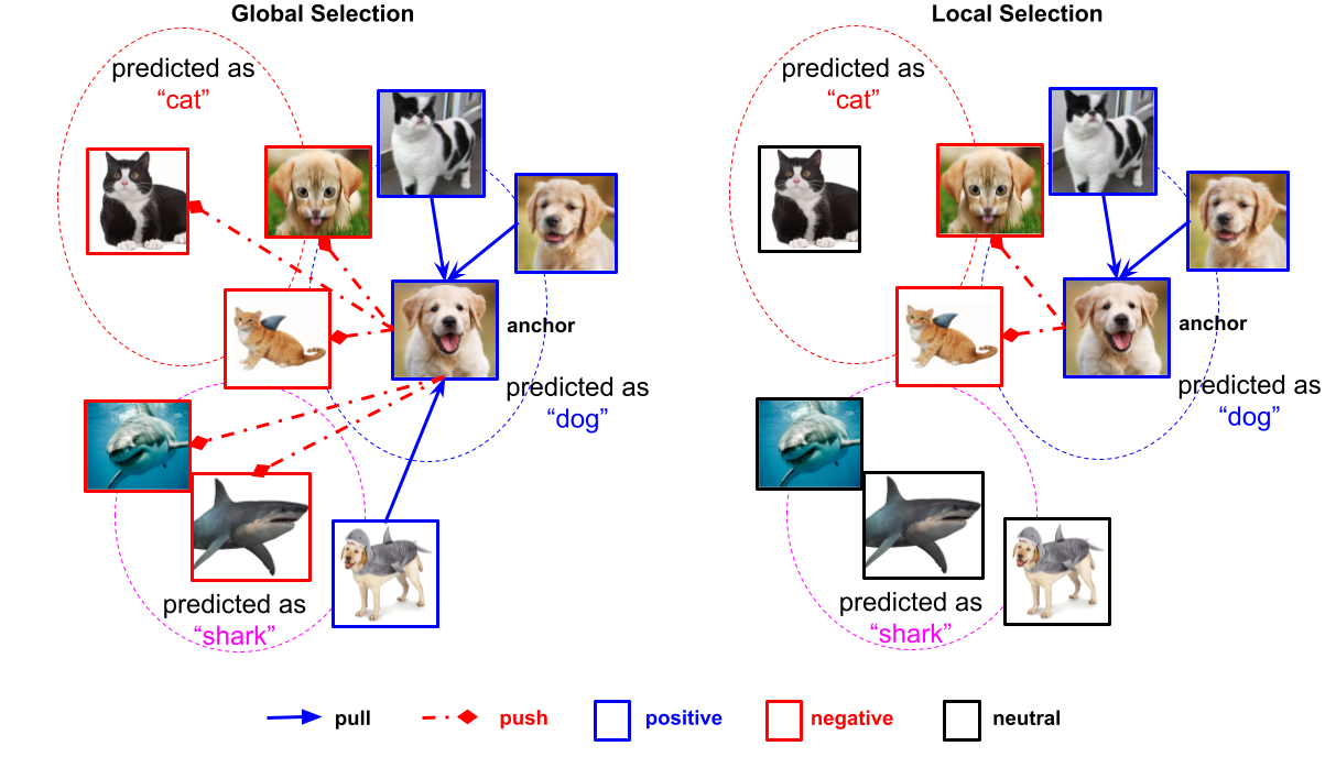
Figure 1: Illustration of ASCL with Global/Local Selection strategies in the latent space. While Global Selection considers all other images in the batch as either positives or negatives, Local Selection nominates the most relevant samples to the anchor when operating contrastive learning. The decision is based on the correlation between the true labels and the predicted labels as in Table 1.

(Q1) Why can CL help to improve the adversarial robustness? To answer this question, we first introduce two kinds of divergences in the latent space: the intra-class divergence measured on benign images and their adversarial examples of the same class and the inter-class divergence measured on those samples of different classes. By comprehensively investigating the behavior of divergence in latent space, our study shows that the robustness of a model can be interpreted by the ratio between the intra- and inter-divergences: The lower the ratio is, the more robustness can be achieved. These observations motivate the idea that a robust model can be achieved by simultaneously contrasting the intra-class divergence between images and their adversarial examples with the inter-class divergence. We provide detailed analysis in Section 2.

(Q2) How to integrate CL with adversarial training in the context of AML? CL originally works with the case where data labels are unavailable, which does not fit the context of AML for classifiers in the supervised setting. The recent research of Supervised Contrastive Learning (SCL) (Khosla et al.,, 2020) extends CL by leveraging label information, where the latent representations from the same class are pulled closer together than those from different classes. While it might seem to be straightforward to apply SCL for AML, we show in this paper that it is highly nontrivial to do so. To this end, we propose Adversarial Supervised Contrastive Learning (ASCL) to tackle this task by developing the following adaptions. Firstly, for an anchor image, we use its adversarial images as the transformed/augmented samples, which is different from the standard data augmentation techniques used in conventional CL methods (Chen et al.,, 2020; Khosla et al.,, 2020). Secondly, we integrate SCL with adversarial training (Madry et al.,, 2018) in addition to the clustering assumption (Chapelle and Zien,, 2005), to enforce compactness in latent space and subsequently improve the adversarial robustness.

(Q3) What are the important factors for the application of the ASCL framework in the context of AML? One of the key steps of CL/SCL is the selecting of positive and negative samples for an anchor image. Although different approaches have been proposed, most of them focus on natural images and can usually be ineffective for AML. Specifically, in a data batch, CL and SCL consider the samples that are not from the same instance or not in the same class of the anchor image as its negative samples, which are hard splits between positive and negative sets, without taking into account the correlation between a sample and the anchor image. This can lead to too many true negative but useless samples which are highly uncorrelated with the anchor in the latent space as illustrated in Figure 1. This issue aggravates with more diverse data and in the AML context, making the original CL/SCL approaches inapplicable. We therefore develop a novel series of strategies for selecting positive and negative samples in our ASCL framework, which judiciously picks the most relevant samples of the anchor that help to further improve adversarial robustness.

By providing the answers to the above research questions, we summarize our contributions in this paper as follows:

1) We provide a comprehensive and insightful understanding of adversarial robustness regarding the divergences in latent space, which sheds light on adapting the CL principle to enhance robustness.

2) We propose a novel Adversarial Supervised Contrastive Learning (ASCL) framework, where the well-established contrastive learning mechanism is leveraged to make the latent space of a classifier more compact, leading to a more robust model against adversarial attacks.

3) By analyzing the intrinsic characteristics of AML, we develop effective strategies for selecting positive and negative samples more judiciously, which are critical to making contrastive learning principle effective in AML by using much less positives and negatives.

4) As shown in extensive experiments, our proposed framework is able to significantly improve a classifier’s robustness, outperforming several adversarial training defense methods against strong attacks while achieving comparable performance with SOTA defenses in the RobustBench (Croce et al.,, 2020).

2 Analysis of Latent Space Divergence

By examining the question “Why can CL help to improve the adversarial robustness?”, we design experiments to show the connection of adversarial robustness to the latent divergence of an anchor and its contrastive samples.

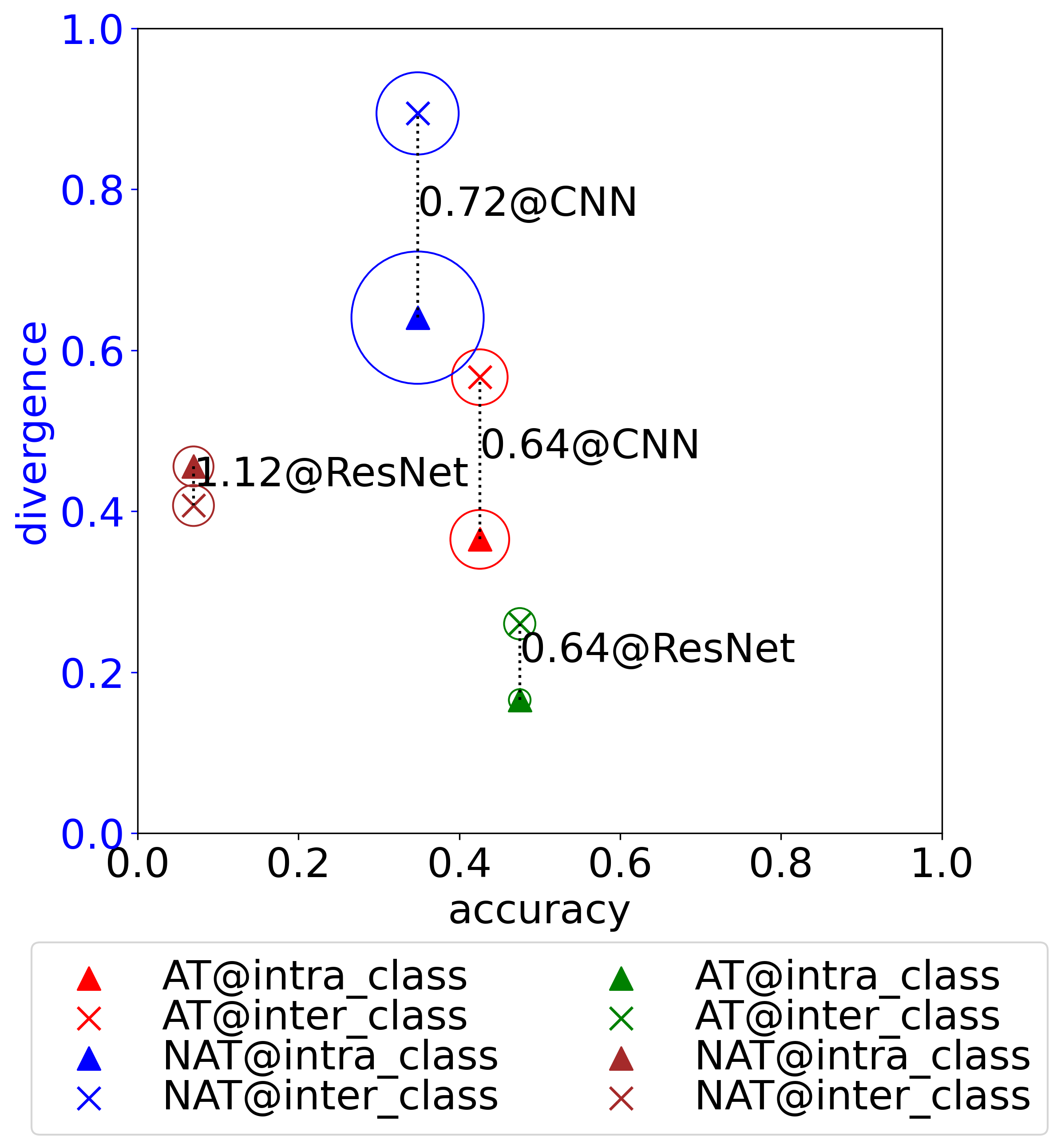
(a) Pairs of Absolute-DIVs with corresponding R-DIV.

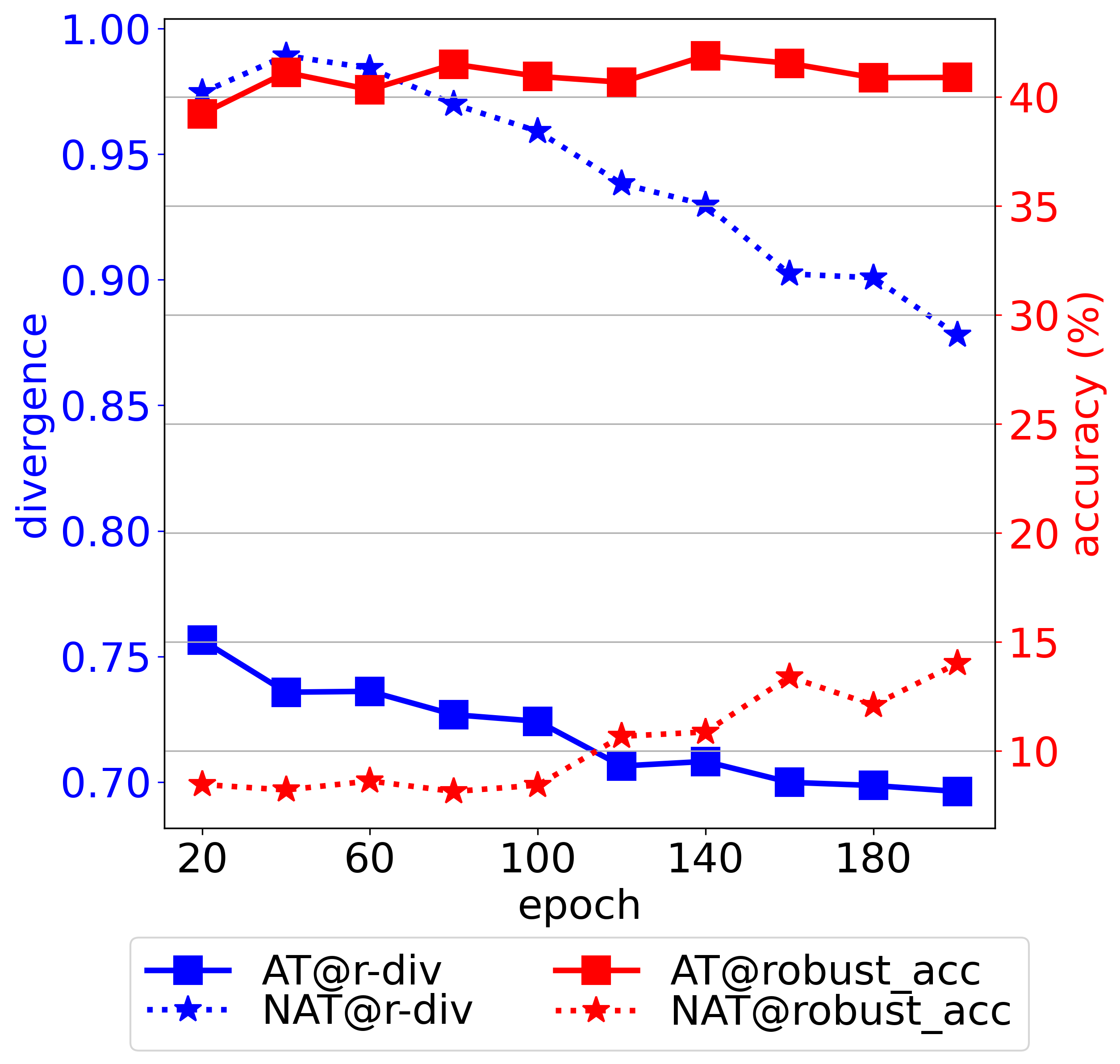
(b) R-DIV over the training progress with standard CNN model.

(c) R-DIV under different attack strengths.

Figure 2: Correlation between the Relative intra-class divergence (R-DIV) and the robust accuracy on the CIFAR10 dataset. The variance of Absolute-DIV in Figure 2a is scaled by 0.2 for better visualization. Using PGD attack with $\epsilon=8/255,\eta=2/255$ with $k=10$ for training and $k=250$ for testing.

Let $\mathcal{\mathcal{B}}=\{\mathbf{x}_{i},\boldsymbol{y}_{i}\}_{i=1}^{N}$ be a batch of benign images where image $\mathbf{x}_{i}$ is associated $\boldsymbol{y}_{i}$. Given an adversarial transformation $\mathcal{T}$ from an adversary $\mathcal{A}$ (e.g., PGD attack in Madry et al., (2018)), we consider two kinds of samples w.r.t. an anchor $\{\mathbf{x}_{i},\boldsymbol{y}_{i}\}$: the positive set $\boldsymbol{X}_{i}^{+}=\{\mathbf{x}_{j},\mathbf{x}_{j}^{\mathcal{T}}\mid j\neq i,\boldsymbol{y}_{j}=\boldsymbol{y}_{i}\}$ including benign examples and their counterparts in the same class with the anchor and the negative set $\boldsymbol{X}_{i}^{-}=\{\mathbf{x}_{j},\mathbf{x}_{j}^{\mathcal{T}}\mid j\neq i,\boldsymbol{y}_{j}\neq\boldsymbol{y}_{i}\}$ including benign examples and their counterparts in different classes with the anchor. We are interested in the latent representations of begin and transformed images at a specific intermediate layer of the neural net classifier $f$. Let us further denote those representations by $\mathbf{z}_{i}$ for benign images and $\mathbf{z}_{i}^{\mathcal{T}}$ for adversarially transformed images according $\mathcal{T}$. We define some types of divergences between benign images and transformed images via transformation $\mathcal{T}$ at some intermediate layers of $f$.

(i) Absolute intra-class divergence: $d_{a}^{+}=\frac{1}{N}\sum_{i=1}^{N}\frac{1}{\left|\boldsymbol{X}_{i}^{+}\right|}\sum_{\mathbf{x}_{j}\in\boldsymbol{X}_{i}^{+}}d(\mathbf{z}_{i},\mathbf{z}_{j})$ (i.e., evaluated based on the positive sets); and absolute inter-class divergence: $d_{a}^{-}=\frac{1}{N}\sum_{i=1}^{N}\frac{1}{\left|\boldsymbol{X}_{i}^{-}\right|}\sum_{\mathbf{x}_{j}\in\boldsymbol{X}_{i}^{-}}d(\mathbf{z}_{i},\mathbf{z}_{j})$ (i.e., evaluated based on the negative sets). Here we note that $d$ is cosine distance between two representations, and $\left|.\right|$ represents the cardinality of a set.

(ii) Relative intra-class divergence (R-DIV): $d_{r}^{+}=\frac{d_{a}^{+}}{d_{a}^{-}}$; hence relative divergence generally represents how large the magnitude of intra-class divergence is relative to the inter-class divergence.

In Figure 2, we conduct an empirical study on the CIFAR-10 dataset to figure out the relationship between R-DIV for adversarial examples and robust accuracy. The findings and observations are very important for us to devise our framework in the sequel. More specifically, we train a CNN and a ResNet20 model in two modes: natural mode (NAT and cannot defend at all) and adversarial training mode (AT and can defend quite well). We observe how robust accuracy together with R-DIV vary with training progress to draw conclusions. The detailed settings and further demonstrations can be found in the supplementary material. Some observations are drawn from our experiment:

(O1) The robustness varies inversely with the relative intra-class divergence between benign images and their adversarial examples (the adversarial R-DIV $d_{r}^{+,adv}$). As shown in Figure 2b, during the training process, the robust accuracy of the AT model tends to improve, which corresponds with a decrease of the adversarial R-DIV $d_{r}^{+,adv}$. Similarly, when the robust accuracy of the NAT model starts increasing at the epoch 100, the adversarial R-DIV $d_{r}^{+,adv}$ starts decreasing. In addition, the robust accuracy of the AT model is significantly higher than that of the NAT model, whilst its $d_{r}^{+,adv}$ is far lower than that of the NAT model. In Figure 2c, we visualize the correlation between the R-DIV and the robust accuracy by generating different attack strengths. It can be seen that there is a common trend such that the lower robust accuracy the higher R-DIV, regardless of the model architecture or defense methods. These observations support our claim of the relation between robust accuracy and R-DIV.

(O2) In Figure 2a, we visualize the absolute intra-class divergence ($d_{a}^{+}$) and the absolute inter-class divergence ($d_{a}^{-}$) for the cases of the NAT/AT models with their corresponding robust accuracies. It can be observed that: (i) in the same architecture, the $d_{a}^{+}$ of the AT model is much smaller than that of NAT model. However, the $d_{a}^{-}$ of the AT model is also much smaller than that of NAT model. It implies that, the AT method helps to compact the representations of intra-class samples, but undesirably makes the representations of inter-class samples closer. (ii) Overall, the relative intra-class divergence of the AT model is smaller than that of the NAT model – which might explain why the NAT model is easy to be attacked, and again confirms our O1.

Conclusions from the observations.

Mao et al., (2019) and Bui et al., (2020) reached a conclusion that the absolute adversarial intra-class divergence $d_{a}^{+}$ is a key factor for robustness against adversarial examples. However, as indicated by our O1, it is only one side of the coin. The reason is that the absolute adversarial intra-class divergence only cares about how far adversarial examples of a class are from their counterpart benign images, and does not pay attention to the inter-divergence to other classes. As analysed in our observation of O2-i, low $d_{a}^{-}$ possibly harms the robust accuracy, because in this case, adversarial examples of other classes are very close to those of the given class. This further indicates that the absolute adversarial inter-class divergence $d_{a}^{-}$ needs to be taken into account and it is necessary to minimize the relative adversarial intra-class divergence $d_{r}^{+}=\frac{d_{a}^{+}}{d_{a}^{-}}$ better controls both the absolute adversarial intra-class divergence and absolute adversarial inter-class divergence for strengthening robustness. The above analytical and empirical study confirms the feasibility of applying SCL to enhance robustness in AML but one can also see that it is non-trivial to develop an appropriate strategy to be the combination effective.

3 Proposed method

In this section, we provide the answer for the question “How to integrate CL with adversarial training in the context of AML?”. We first propose an adapted version of SCL which we call Adversarial Supervised Contrastive Learning (ASCL) for the AML problem. We then introduce three sample selection strategies to nominate the most relevant positives and negatives to the anchor, which further improve robustness with much fewer samples.

3.1 Adversarial Supervised Contrastive Learning

Terminologies.

We consider a prediction model $h(\mathbf{x})=g(f(\mathbf{x}))$ where $f()$ is the encoder which outputs the latent representation $\mathbf{z}=f(\mathbf{x})$ and $g()$ is the classifier upon the latent $\mathbf{z}$. Also we have a batch of N pairs $\{\mathbf{x}_{i},\boldsymbol{y}_{i}\}_{i=1}^{N}$ of benign images and their labels. With an adversarial transformation $\mathcal{A}$ (e.g., PGD), each pair $\{\mathbf{x}_{i},\boldsymbol{y}_{i}\}$ has two corresponding sets, a positive set $\boldsymbol{X}_{i}^{+}=\{\mathbf{x}_{j},\mathbf{x}_{j}^{a}\mid j\neq i,\boldsymbol{y}_{j}=\boldsymbol{y}_{i}\}$ and a negative set $\boldsymbol{X}_{i}^{-}=\{\mathbf{x}_{j},\mathbf{x}_{j}^{a}\mid j\neq i,\boldsymbol{y}_{j}\neq\boldsymbol{y}_{i}\}$. We then have the corresponding sets in the latent space $\boldsymbol{Z}_{i}^{+}=\{f(\mathbf{x}_{j})\mid\mathbf{x}_{j}\in\boldsymbol{X}_{i}^{+}\}$ and $\boldsymbol{Z}_{i}^{-}=\{f(\mathbf{x}_{j})\mid\mathbf{x}_{j}\in\boldsymbol{X}_{i}^{-}\}$.

Supervised Contrastive Loss.

The supervised contrastive loss for an anchor $\mathbf{x}_{i}$ as follow:

$$\mathcal{L}_{i}^{\text{scl}}=\frac{-1}{\left|\boldsymbol{Z}_{i}^{+}\right|+1}\underset{\mathbf{z}_{j}\in\boldsymbol{Z}_{i}^{+}\cup\{\mathbf{z}_{i}^{a}\}}{\sum}\log\frac{e^{\frac{sim(\mathbf{z}_{j},\mathbf{z}_{i})}{\tau}}}{\underset{\mathbf{z}_{k}\in\boldsymbol{Z}_{i}^{+}\cup\boldsymbol{Z}_{i}^{-}\cup\{\mathbf{z}_{i}^{a}\}}{\sum}e^{\frac{sim(\mathbf{z}_{k},\mathbf{z}_{i})}{\tau}}}$$ (1)

where $sim(\mathbf{z}_{j},\mathbf{z}_{i})$ represents the similarity metric between two latent representations and $\tau$ is a temperature parameter. It is worth noting that there are two changes in our SCL loss compared with the original one in Khosla et al., (2020). Firstly, $sim(\mathbf{z}_{j},\mathbf{z}_{i})$ is a general form of similarity, which can be any similarity metric such as cosine similarity $\frac{\mathbf{z}_{j}\cdot\mathbf{z}i}{\left\|\mathbf{z}_{j}\right\|\times\left\|\mathbf{z}_{i}\right\|}$ or Lp norm $-\left|\mathbf{z}_{j}-\mathbf{z}_{i}\right|_{p}$. Secondly, in term of terminology, in Khosla et al., (2020), the positive set was defined including those samples in the same class with the anchor $\mathbf{x}_{i}$ (e.g. $\boldsymbol{X}_{i}^{+}$) and the anchor’s transformation $\mathbf{x}_{i}^{a}$. However, in our paper, we want to emphasize the importance of the anchor’s transformation, therefore, we use two separate terminologies $\boldsymbol{X}_{i}^{+}$ and $\{\mathbf{x}_{i}^{a}\}$. Similarly, the SCL loss for an anchor $\mathbf{x}_{i}^{a}$ as follow:

$$\mathcal{L}_{i}^{\text{a,scl}}=\frac{-1}{\left|\boldsymbol{Z}_{i}^{+}\right|+1}\underset{\mathbf{z}_{j}\in\boldsymbol{Z}_{i}^{+}\cup\{\mathbf{z}_{i}\}}{\sum}\log\frac{e^{\frac{sim(\mathbf{z}_{j},\mathbf{z}_{i})}{\tau}}}{\underset{\mathbf{z}_{k}\in\boldsymbol{Z}_{i}^{+}\cup\boldsymbol{Z}_{i}^{-}\cup\{\mathbf{z}_{i}\}}{\sum}e^{\frac{sim(\mathbf{z}_{k},\mathbf{z}_{i})}{\tau}}}$$ (2)

The average SCL loss over a batch is as follows:

$$\mathcal{L}^{\text{SCL}}=\frac{1}{N}\sum_{i=1}^{N}\left(\mathcal{L}_{i}^{\text{scl}}+\mathcal{L}_{i}^{\text{a,scl}}\right)$$ (3)

As mentioned in Khosla et al., (2020), there is a major advantage of SCL compared with Self-Supervised CL (SSCL) in the context of regular machine learning. Unlike SSCL in which each anchor has only single positive sample, SCL takes advantages of the labels to have many positives in the same batch size N. This strategy helps to reduce the false negative cases in SSCL when two samples in the same class are pushed apart. As shown in Khosla et al., (2020), SCL training is more stable than SSCL and also achieves better performance.

Adaptations in the context of AML.

However, original SCL is not sufficient to achieve adversarial robustness. In the context of adversarial machine learning, we need the following adaptations to improve the adversarial robustness:

(i) As shown in Table 1 in Kim et al., (2020), the original SCL slightly improves the robustness of a standard model but cannot defend strong adversarial attacks. Therefore, we use an adversary $\mathcal{A}$ (e.g., PGD) as the transformation $\mathcal{T}$ instead of the traditional data augmentation (e.g., combination of random cropping and random jittering) as in other contrastive learning frameworks (Chen et al.,, 2020; Khosla et al.,, 2020; He et al.,, 2020). This helps to reduce the divergence in latent representations of a benign image and its adversarial example directly.

(ii) We apply SCL as a regularization on top of the Adversarial Training (AT) method (Madry et al.,, 2018; Zhang et al.,, 2019; Shafahi et al.,, 2019; Xie et al.,, 2020). Therefore, instead of pre-training the encoder $f()$ with contrastive learning loss as in previous work, we can optimize the AT and the SCL simultaneously. The AT objective function with the cross-entropy loss $\mathcal{C}()$ is as follows:

$$\mathcal{L}^{AT}=\frac{1}{N}\sum_{i=1}^{N}\mathcal{C}\left(h(\mathbf{x}_{i}),\boldsymbol{y}_{i}\right)+\mathcal{C}\left(h(\mathbf{x}_{i}^{a}),\boldsymbol{y}_{i}\right)$$ (4)

Regularization on the prediction space.

The clustering assumption (Chapelle and Zien,, 2005) is a technique that encourages the classifier to preserve its predictions for data examples in a cluster. Theoretically, the clustering assumption enforces the decision boundary of a given classifier to lie in the gap among the data clusters and never cross over any clusters. As shown in Chen et al., (2020); Khosla et al., (2020), with the help of CL, latent representations of those samples in the same class form into clusters. Therefore, coupling our SCL framework with the clustering assumption can help to increase the margin from a data sample to the decision boundary. To enforce the clustering assumption, we use Virtual Adversarial Training (VAT) (Miyato et al.,, 2019) to maintain the classifier smoothness:

$$\mathcal{L}^{\text{VAT}}=\frac{1}{N}\sum_{i=1}^{N}D_{KL}\left(h(\mathbf{x}_{i})\parallel h(\mathbf{x}_{i}^{a})\right)$$ (5)

Putting it all together.

We combine the relevant terms to the final objective function of our framework which we name as Adversarial Supervised Contrastive Learning (ASCL) as follows:

$$\mathcal{L}=\mathcal{L}^{\text{AT}}+\lambda^{\text{SCL}}\mathcal{L}^{\text{SCL}}+\lambda^{\text{VAT}}\mathcal{L}^{\text{VAT}}$$ (6)

where $\lambda^{\text{SCL}}$ and $\lambda^{\text{VAT}}$ are hyper-parameters to control the SCL loss and VAT loss, respectively. As mentioned in the observation (O2), minimizing the AT loss $\mathcal{L}^{AT}$ alone compresses not only the representations of intra-class clusters but also reduces the inter-class distance, which hurts the natural discrimination. Therefore, coupling with $\mathcal{L}^{SCL}$ can compensate the aforementioned weakness by simultaneously minimizing the intra-class divergence and maximizing the inter-class divergence. Finally, by forcing predictions of intra-class samples to be close, the VAT regularization $\mathcal{L}^{VAT}$ help to maintain the classifier smoothness and further improve the robustness. In addition to the intuitive analysis, we also provide an empirical ablation study to further understand the contribution of each component in the supplementary material.

3.2 Global and Local Selection Strategies

Table 1: Definitions of positives and negatives with Global Selection and Local Selection strategies given an anchor $\{\mathbf{x}_{i},\boldsymbol{y}_{i}\}$ and a predicted label $p=\text{argmax}\;h(\mathbf{x})$, $p^{a}=\text{argmax}\;h(\mathbf{x}^{a})$

	$\boldsymbol{X}_{i}^{+}$	$\boldsymbol{X}_{i}^{-}$
Global	$\{\mathbf{x}_{j},\mathbf{x}_{j}^{a}\mid j\neq i,\boldsymbol{y}_{j}=\boldsymbol{y}_{i}\}$	$\{\mathbf{x}_{j},\mathbf{x}_{j}^{a}\mid j\neq i,\boldsymbol{y}_{j}\neq\boldsymbol{y}_{i}\}$
Hard-LS	$\{\mathbf{x}_{j},\mathbf{x}_{j}^{a}\mid j\neq i,\boldsymbol{y}_{j}=\boldsymbol{y}_{i}\}$	$\{\mathbf{x}_{j}\mid j\neq i,\boldsymbol{y}_{j}\neq\boldsymbol{y}_{i},p_{j}=\boldsymbol{y}_{i}\}\cup\{\mathbf{x}_{j}^{a}\mid j\neq i,\boldsymbol{y}_{j}\neq\boldsymbol{y}_{i},p_{j}^{a}=\boldsymbol{y}_{i}\}$
Soft-LS	$\{\mathbf{x}_{j},\mathbf{x}_{j}^{a}\mid j\neq i,\boldsymbol{y}_{j}=\boldsymbol{y}_{i}\}$	$\{\mathbf{x}_{j}\mid j\neq i,\boldsymbol{y}_{j}\neq\boldsymbol{y}_{i},p_{j}=p_{i}\}\cup\{\mathbf{x}_{j}^{a}\mid j\neq i,\boldsymbol{y}_{j}\neq\boldsymbol{y}_{i},p_{j}^{a}=p_{i}\}$
Leaked-LS	$\{\mathbf{x}_{j}\mid j\neq i,\boldsymbol{y}_{j}=\boldsymbol{y}_{i},p_{j}=p_{i}\}\cup\{\mathbf{x}_{j}^{a}\mid j\neq i,\boldsymbol{y}_{j}=\boldsymbol{y}_{i},p_{j}^{a}=p_{i}\}$	$\{\mathbf{x}_{j}\mid j\neq i,\boldsymbol{y}_{j}\neq\boldsymbol{y}_{i},p_{j}=p_{i}\}\cup\{\mathbf{x}_{j}^{a}\mid j\neq i,\boldsymbol{y}_{j}\neq\boldsymbol{y}_{i},p_{j}^{a}=p_{i}\}$

Global Selection.

The SCL as in Equations 1,2 can be understood as SCL with a Global Selection strategy, where each anchor $\mathbf{x}_{i}$ takes all other samples in the current batch into account and splits them into a positive set $\boldsymbol{X}_{i}^{+}$ and a negative set $\boldsymbol{X}_{i}^{-}$. For example, as illustrated in Figure 1, given an anchor, with the help of SCL, it will push away all negatives and pull all positives regardless of their correlation in the space. However, there are two issues of this strategy:

(I1) The high inter-class divergence issue of a diverse dataset. Specifically, there are true negative (but uncorrelated) samples which are very different in appearance (e.g., an anchor-dog and negative samples-sharks) and latent representations. Therefore, pushing them away does not make any contribution to the learning other than making it more unstable. The number of uncorrelated negatives is increased when the dataset is more diverse.

(I2) The high intra-class divergence issue when the dataset is very diverse in some classes. For example, a class “dog” in the ImageNet dataset may include many sub-classes (breeds) of dog. Specifically, there are true positive (but uncorrelated) samples which are in the same class with the anchor but different in appearance. In the context of AML, two samples in the same class (e.g., “dog”) can be attacked to be very different classes (e.g., one to the class “cat”, one to the class “shark”), therefore the latent representations of their adversarial examples are even more uncorrelated.

Local Selection.

Based on the above analysis, we leverage label supervision to propose a series of Local Selection (LS) strategies for the SCL framework, which consider local and important samples only and ignore other samples in the batch as illustrated in Figure 1. They are Hard-LS, Soft-LS and Leaked-LS as defined in Table 1.

More specifically, in Hard-LS and Soft-LS, we consider the same set of positives as in Global Selection. However, we filter out the true negative but uncorrelated samples by only considering those are predicted as similar to the anchor’s true label (Hard-LS) or to the anchor’s predicted label (Soft-LS). These two strategies are to deal with the issue (I1) by choosing negative samples that have most correlation with the current anchor. Because they are very close in prediction space, their representation is likely high correlated with the anchor’s representation.

In Leaked-LS, we add an additional constraint on the positive set to deal with the issue (I2). Specifically, we filter out the true positive but uncorrelated samples by only choosing those are currently predicted as similar to the anchor’s prediction. It is worth noting that, the additional constraint is applied on the positive set $\boldsymbol{X}_{i}^{+}$ only. It means that, each anchor $\mathbf{x}_{i}$ and its adversarial example $\mathbf{x}_{i}^{a}$ are always pulled close together. However, instead of pulling all other positive samples in current batch, we only pull those samples which are close with the anchor’s representation to further support and stabilize the contrastive learning.

From a practical perspective, as later shown in the experimental section, ASCL with Leaked-Local Selection (Leaked ASCL) improves the robustness over that with Global Selection most notably, and with much fewer positive and negative samples. It has been shown that, optimal negative samples for contrastive learning are task-dependent which guide representations towards task-relevant features that improve performance (Tian et al.,, 2020; Frankle et al.,, 2020). However, while these previous works focused on unsupervised-setting, our Local-ASCL is the first work to leverage supervision to select not only optimal negative samples but also optimal positive samples for robust classification task.

4 Experiments

In this section, we first introduce the experimental setting for adversarial attacks and defenses. We then provide an extensive robustness evaluation between our best method (which is Leaked-ASCL) with other defenses to demonstrate the significant improvement of ours. Finally, we empirically answer the question “What are the important factors for the application of the ASCL framework in the context of AML?” through our experiments. We provide a comparison among Global/Local Selection strategies and show that the Leaked-ASCL not only outperforms the Global ASCL but also makes use of much fewer positives and negatives. An ablation study to investigate the importance of each component to the performance can be found in the supplementary material.

4.1 Experimental Setting

General Setting.

We use CIFAR10 and CIFAR100 (Krizhevsky et al.,, 2009) as the benchmark datasets in our experiment. Both datasets have 50,000 training images and 10,000 test images. However, while the CIFAR10 dataset has 10 classes, CIFAR100 is more diverse with 100 classes. The inputs were normalized to $[0,1]$. We apply random horizontal flips and random shifts with scale $10\%$ for data augmentation as used in Pang et al., (2019). We use four architectures including standard CNN, ResNet18/20 (He et al.,, 2016) and WideResNet-34-10 (Zagoruyko and Komodakis,, 2016) in our experiment. The architecture and training setting for each dataset are provided in our supplementary material.

Contrastive Learning Setting.

We choose the penultimate layer ($l_{y}^{-1})$ as the intermediate layer to apply our regularization. The analytical study for the effect of choosing projection head in the context of AML can be found in the supplementary material. In the main paper, we report the experimental results without the projection head. The temperature $\tau=0.07$ as in Khosla et al., (2020).

Attack Setting.

We use different state-of-the-art attacks to evaluate the defense methods including: (i) PGD attack which is a gradient based attack. We use $k=250,\epsilon=8/255,\eta=2/255$ for the CIFAR10 dataset and $k=250,\epsilon=0.01,\eta=0.001$ for the CIFAR100 dataset. We use two versions of the PGD attack: the non-targeted PGD attack (PGD) and the multi-targeted PGD attack (mPGD). (ii) Auto-Attack (Croce and Hein,, 2020) which is an ensemble based attack. We use $\epsilon=8/255$ for the CIFAR10 dataset and $\epsilon=0.01$ for the CIFAR100 dataset, both with the standard version of Auto-Attack (AA), which is an ensemble of four different attacks. The distortion metric we use in our experiments is $l_{\infty}$ for all measures. We use the full test set for the attacks (i) and 1000 test samples for the attacks (ii).

Generating Adversarial Examples for Defenders.

We employ PGD as the stochastic adversary to generate adversarial examples. These adversarial examples have been used as transformations of benign images in our contrastive framework. Specifically, the configuration for the CIFAR10 dataset is $k=10,\epsilon=8/255,\eta=2/255$ and that for the CIFAR100 dataset is $k=10,\epsilon=0.01,\eta=0.001$.

Baseline methods.

Most closely related to our work is ADR (Bui et al.,, 2020) which also aims to realize compactness in the latent space to improve robustness in the supervised setting. We also compare with RoCL-TRADES (Kim et al.,, 2020) and ACL-DS (Jiang et al.,, 2020) which adversarially pre-trains with adversarial examples founded by Self-Supervised Contrastive loss and post-trains with standard supervised adversarial training.

4.2 Robustness evaluation

Table 2: Robustness evaluation on the CIFAR10 and CIFAR100 datasets with ResNet20 architecture. Ours is Leaked-ASCL variant. GAP represents the average gap of robust accuracies between ours and the compared method.

	CIFAR10						CIFAR100
	Nat.	PGD	mPGD	AA	GAP		Nat.	PGD	mPGD	AA	GAP
ADV	78.8	48.1	36.4	36.1	5.37		60.7	35.7	25.3	25.7	6.27
TRADES	76.1	51.9	38.2	36.3	3.43		59.0	37.2	25.3	25.7	5.77
ADR	76.8	51.5	38.9	38.6	2.57		59.1	40.0	29.1	28.6	2.60
Ours	75.5	53.7	41.0	42.0	0		59.0	42.5	31.1	31.9	0

Table 3: Robustness evaluation against Auto-Attack with ResNet18 and WideResNet on the full test set of CIFAR10 dataset. $\star$ Results are copied from Croce et al., (2020). $\ddagger$ Results are copied from original papers, using a larger batch size (bs). $\ast$ Omit the cross-entropy loss of natural images and VAT loss. Detail can be found in the supplementary material.

	Model	Nat	AA	PGD
Ours $\ast$	WideResNet	87.70	52.80	54.05
Zhang et al., (2020) $\star$	WideResNet	84.52	53.51	-
Huang et al., (2020) $\star$	WideResNet	83.48	53.34	-
Zhang et al., (2019) $\star$	WideResNet	84.92	53.08	-
Cui et al., (2021) $\star$	WideResNet	88.22	52.86	-
Ours $\ast$	ResNet18	85.02	50.31	53.40
ACL-DS (bs=512) $\ddagger$	ResNet18	82.19	-	52.82
RoCL-TRADES (bs=256) $\ddagger$	ResNet18	84.55	-	43.85

We conduct extensive evaluations to demonstrate the advantages of our method (Leaked-ASCL variant) over other defenses. Table 2 shows the robustness comparison on the CIFAR10 and CIFAR100 datasets with ResNet20 architecture. It can be seen that our method achieves much better robustness than the baseline methods on both datasets. More specifically, on the CIFAR10 dataset, the average gaps of robust accuracies against three attacks (PGD, mPGD and AA) between ours and ADR, TRADES, and ADV are $2.57\%$, $3.43\%$ and $5.37\%$, respectively. The similar gaps for the CIFAR100 dataset are $2.60\%$, $5.77\%$ and $6.27\%$, respectively. Figure 3 shows the tradeoff between natural accuracy and robust accuracies when increasing perturbation magnitude. It can be seen that simply increasing the magnitude of adversarial examples cannot reach our performance even with a fine-range of perturbation. With the same level of natural accuracy, our method outperforms the baseline by around 5% which again emphasizes the advantage of our method. Finally, we compare our method with recently listed methods on the RobustBench (Croce et al.,, 2020) which have a similar setting (e.g., without additional data) as shown in Table 3. With WideResNet architecture, our method achieves $52.80\%$ robust accuracy against Auto-Attack and 87.70% natural accuracy which is comparable with the SOTA method from Cui et al., (2021). Compare to the best robust method from Zhang et al., (2020), our method has 0.7% lower in robust accuracy but 3.2% higher in natural performance. With a smaller batch size, our method still achieves much better performance than RoCL and ACL which are two SOTA self-supervised contrastive learning based defenses.

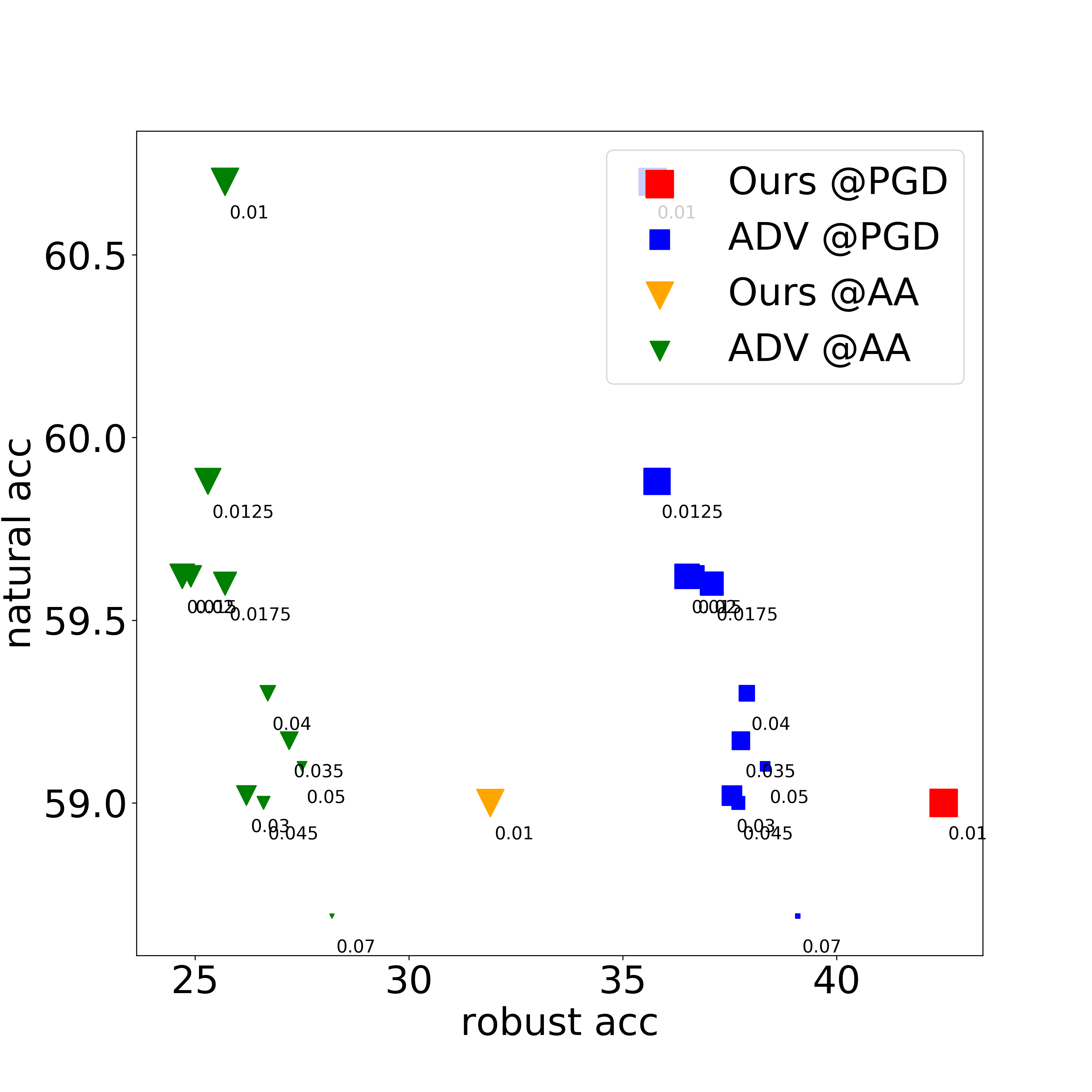
Figure 3: Tradeoff between natural/robust accuracies when increasing perturbation magnitude (specified beside markers). For better visualization, bigger marker indicates smaller perturbation. Ours is Leaked-ASCL.

4.3 Global and Local Selection strategies

In this subsection, we compare the effect of different global/local selection strategies to the final performance. The comparison in Table 4 shows that while the Hard-ASCL and Soft-ASCL show a small improvement over ASCL, the Leaked-ASCL achieves the best robustness compared with other strategies.

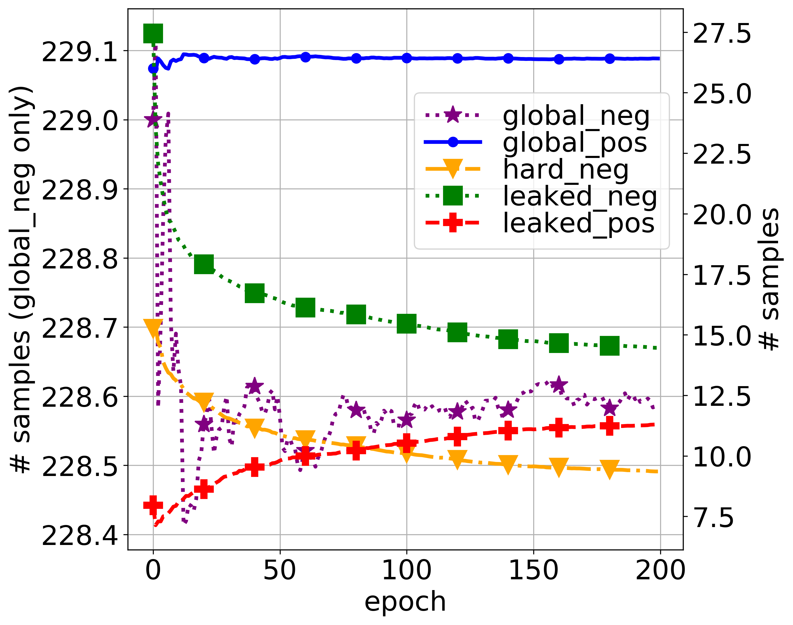
(a) Global/Local

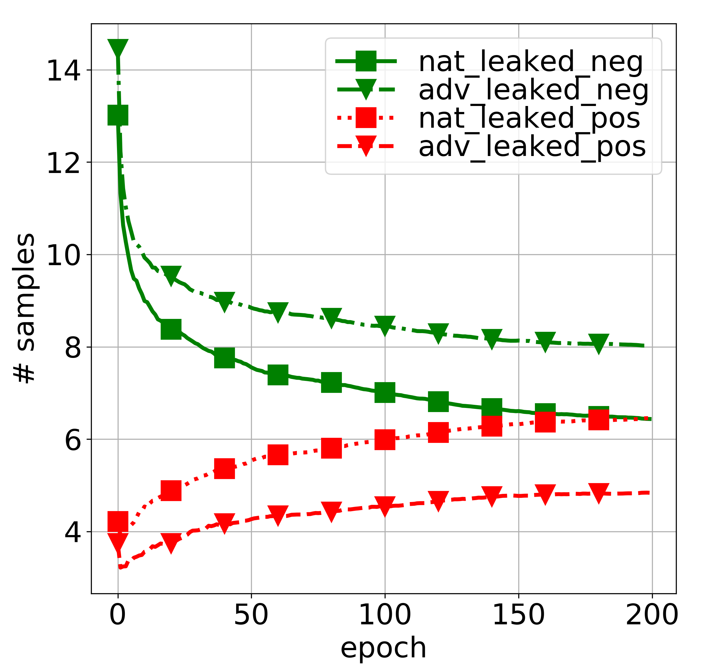
(b) Detail of Leaked Local

Figure 4: Number of positives and negatives with different Global/Local Selection strategy on CIFAR10 dataset with batch size 128

Table 4: Comparison among Global/Local Selection Strategies on the CIFAR10 dataset with ResNet20

	Nat.	PGD	mPGD	AA
(Global) ASCL	76.4	52.7	40.4	40.9
Hard-ASCL	75.5	53.1	41.0	41.3
Soft-ASCL	75.5	53.4	40.6	40.4
Leaked-ASCL	75.5	53.7	41.0	42.0

We also measure the average number of positive and negatives samples per batch corresponding with different selection strategies as shown in Figure 4a. With batch size 128, we have a total of 256 samples per batch including benign images and their adversarial examples. It can be seen that, the average positives and negatives by the Global Selection are stable at 26.4 and 228.6, respectively. In contrast, the number of positives and negatives by the Leaked-LS vary corresponding with the current performance of the model. More specifically, there are four advantages of the Leaked-LS over the Global Selection:

(i) at the beginning of training, approximately 7.5 positive samples and 25 negative samples were selected. This is because of the low classification performance of the model. Moreover, the strength of the contrastive loss is directly proportional with the size of the positive set. Therefore, with a small positive set, the contrastive loss is weak in comparison with other components of ASCL. This helps the model focuses more on improving the classification performance first.

(ii) when the model is improved, the number of positive samples is increased, while the number of negative samples is decreased significantly. In addition to the bigger positive set, the contrastive loss become stronger in comparison with other components. This helps the model now focus more on contrastive learning and learning the compact latent representation.

(iii) unlike Global Selection, Leaked-LS considers natural images and adversarial images differently based on their hardness to the current anchor. As shown in Figure 4b, there are more adversarial images than natural images in the negative set, which helps the encoder focus to contrast the anchor with the adversarial images.

(iv) at the last epoch, Leaked-LS chooses only 11.3 positives and 14.3 negatives, which equate to $42.8\%$ and $6.3\%$ of the positive set and negative set with the Global Selection strategy, respectively.

4.4 Why do ASCL and Local-ASCL improve adversarial robustness

In this subsection, we connect with the hypothesis in Section 2 to explain why our ASCL and especially our Leaked-ASCL help to improve adversarial robustness. Figure 5 shows the Relative intra-class divergence (R-DIV) and robust accuracy under PGD attack $\{k=250,\eta=2/255\}$ with different attack strengths $\epsilon$. It can be seen that (i) our ASCL and Leaked-ASCL have lower R-DIV than baseline methods, and Leaked-ASCL achieves the lowest measure, (ii) consequently, our ASCL and Leaked-ASCL achieves better robust accuracy than baseline methods. Leaked-ASCL achieve the best performance regardless of attack scenarios. The experimental results concur with the proposed correlation between the Relative intra-class divergence and the adversarial robustness as pointed out in Section 2. Our methods help the representations of intra-class samples to be more compact while increasing the margin between inter-class clusters, and therefore improve the robustness.

(a) R-DIV

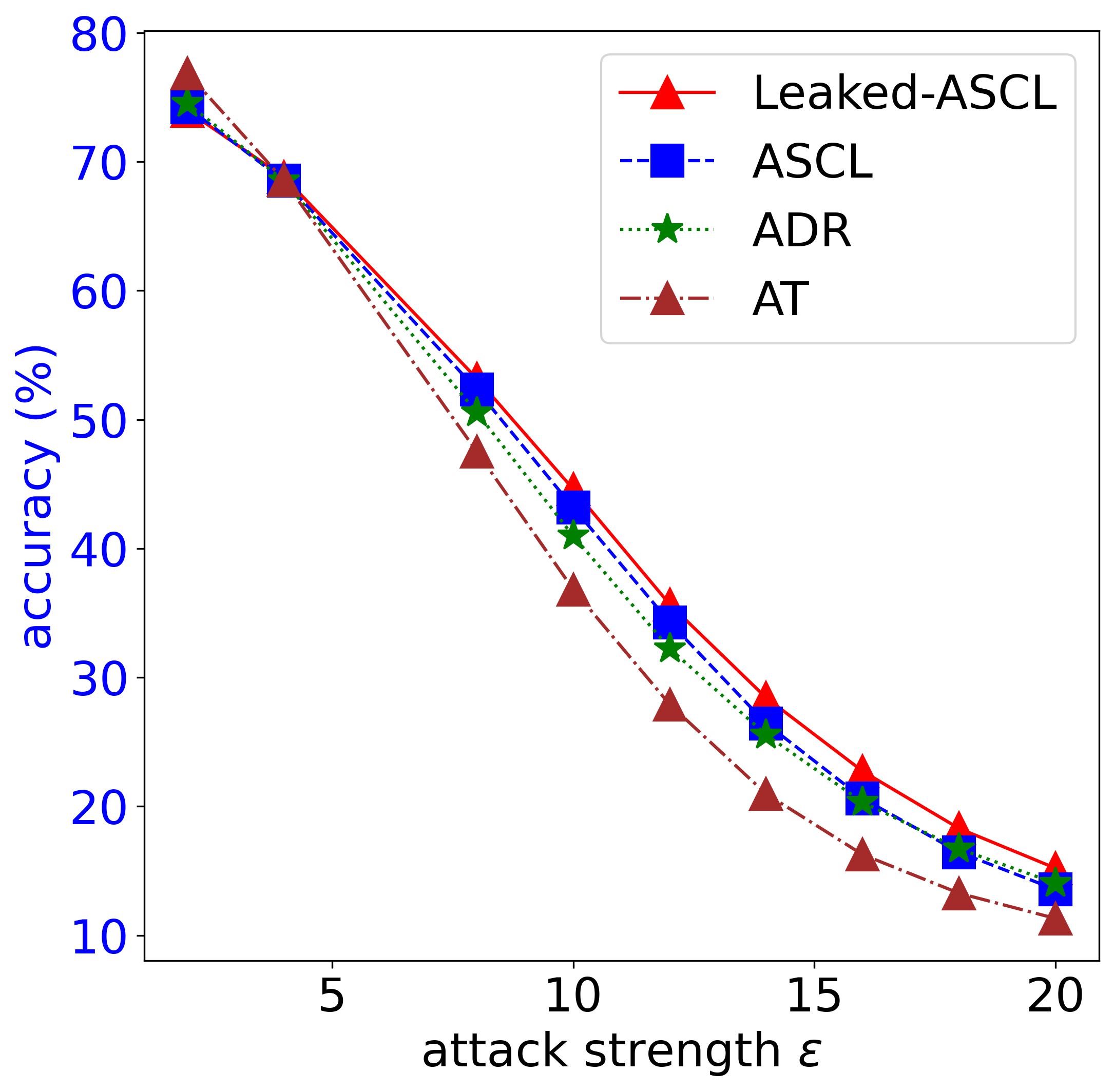
(b) Robust accuracy

Figure 5: R-DIV and robust accuracy under different attack strengths on CIFAR10 with ResNet20.

5 Conclusion

In this paper, we have shown the connection between robust accuracy and the divergence in latent spaces. We demonstrated that contrastive learning can be applied to improve adversarial robustness by reducing the intra-instance divergence while maintaining the inter-class divergence. Moreover, we have shown that, instead of using all negatives and positives as per the regular contrastive learning framework, by judiciously picking highly correlated samples, we can further improve the adversarial robustness.

Supplementary material of “Understanding and Achieving Efficient Robustness with Adversarial Supervised Contrastive Learning”

This supplementary material provides technical and experimental details as well as auxiliary aspects to complement the main paper. Briefly, it contains the following:

• Section 6: Experimental setting.

• Section 7: Additional analysis of latent space divergence as well as t-SNE visualization.

• Section 8: Additional experimental results which includes analysis of projection head in Section 8.1, contribution of each component in Section 8.2, image samples from Global and Local Selection strategies in Section 8.3.

• Section 9: Discussion on the background, related works, and the necessity of our formulations for delivering our method.

6 Experimental setting

General Setting.

We use CIFAR10 and CIFAR100 (Krizhevsky et al.,, 2009) as the benchmark datasets in our experiment. Both datasets have 50,000 training images and 10,000 test images. However, while the CIFAR10 dataset has 10 classes, CIFAR100 is more diverse with 100 classes. The training time is 200 epochs for both CIFAR10 and CIFAR100 datasets with batch size 128. The inputs were normalized to $[0,1]$. We apply random horizontal flips and random shifts with scale $10\%$ for data augmentation as used in Pang et al., (2019).

We use four architectures including standard CNN, ResNet18/20 (He et al.,, 2016) and WideResNet-34-10 (Zagoruyko and Komodakis,, 2016) in our experiment. The standard CNN architecture has 4 convolution layers followed by 3 FC layers as described in Carlini and Wagner, (2017). For ResNet20 architectures, we use the same training setting as in Pang et al., (2019). More specifically, we use Adam optimizer, with learning rate $10^{-3},10^{-4},10^{-5},10^{-6}$ at epoch 0th, 80th, 120th, and 160th, respectively. We use Adam optimization with learning rate $10^{-3}$ for training the standard CNN architecture.

For ResNet18 and WideResNet architectures, we use the same training setting as in Pang et al., (2020). More specifically, we use SGD optimizer, with momentum $5\times 10^{-4}$, with learning rate $10^{-1},10^{-2},10^{-3}$ at epoch 0th, 100th and 150th, respectively. It is a worth noting that, there are some modifications in the experiment in Table 3 to match the performance as in RobustBench: (i) we omit the cross-entropy loss of natural images in Eq. (4), so that the model sacrifices natural performance to gain more robust performance. The AT objective function becomes: $\mathcal{L}^{AT}=\frac{1}{N}\sum_{i=1}^{N}\mathcal{C}\left(h(\mathbf{x}_{i}^{a}),\boldsymbol{y}_{i}\right)$ which is similar as in Pang et al., (2020). (ii) we omit the VAT loss to show that the improvement truly comes from the contribution of the adversarial contrastive loss.

Contrastive Learning Setting.

We apply the contrastive learning on the intermediate layer $(l_{y}^{-1})$ which is intermediately followed by the last FC layer of either CNN or ResNet/WideResNet architectures. The analytical study for the effect of choosing projection head in the context of AML can be found in Section 8.1. In the main paper, we report the experimental results without the projection head. The temperature $\tau=0.07$ as in Khosla et al., (2020).

Attack Setting.

We use different state-of-the-art attacks to evaluate the defense methods including: (i) PGD attack which is a gradient based attack. We use $k=250,\epsilon=8/255,\eta=2/255$ for the CIFAR10 dataset and $k=250,\epsilon=0.01,\eta=0.001$ for the CIFAR100 dataset. We use two versions of the PGD attack: the non-targeted PGD attack (PGD) and the multi-targeted PGD attack (mPGD). (ii) Auto-Attack (Croce and Hein,, 2020) which is an ensemble based attack. We use $\epsilon=8/255$ for the CIFAR10 dataset and $\epsilon=0.01$ for the CIFAR100 dataset, both with the standard version of Auto-Attack (AA), which is an ensemble of four different attacks. The distortion metric we use in our experiments is $l_{\infty}$ for all measures. We use the full test set for the attacks (i) and 1000 test samples for the attacks (ii).

Generating Adversarial Examples for Defenders.

We employ PGD as the stochastic adversary to generate adversarial examples. These adversarial examples have been used as transformations of benign images in our contrastive framework. Specifically, the configuration for the CIFAR10 dataset is $k=10,\epsilon=8/255,\eta=2/255$ and that for the CIFAR100 dataset is $k=10,\epsilon=0.01,\eta=0.001$.

7 Additional Analysis of Latent Space Divergence

Experimental setting.

The training setting has been described in Section 6. Because the intra-class/inter-class divergences are averagely calculated on all $N^{2}$ pairs of latent representations which is over our computational capacity, therefore, we alternately calculate these divergences on a mini-batch (128) and take the average over all mini-batches.

Additional evaluation.

In addition to the comparison in Section 4.2, we provide a further evaluation on R-DIV and robust accuracy on the CIFAR10 dataset with ResNet20 architecture, under PGD attack $\{\epsilon=8/255,\eta=2/255,k=250\}$ as shown in Figure 6. It can be observed that (i) the value of R-DIV decreases in order from AT (0.64), ADR (0.63), ASCL (0.49), Leaked-ASCL (0.48), respectively. On the other hand, the robust accuracy increases in the same order. (ii) ASCL has much higher absolute intra-class divergence and inter-class divergence than ADR and AT methods, however, ASCL has much lower R-DIV comparing with two baseline methods, therefore, explaining its higher robust accuracy. This result is similar with the comparison on Figure 2.a and the observation O2-i in the main paper and further confirm our conclusion such that “the robustness varies inversely with the relative intra-class divergence between benign images and their adversarial examples”.

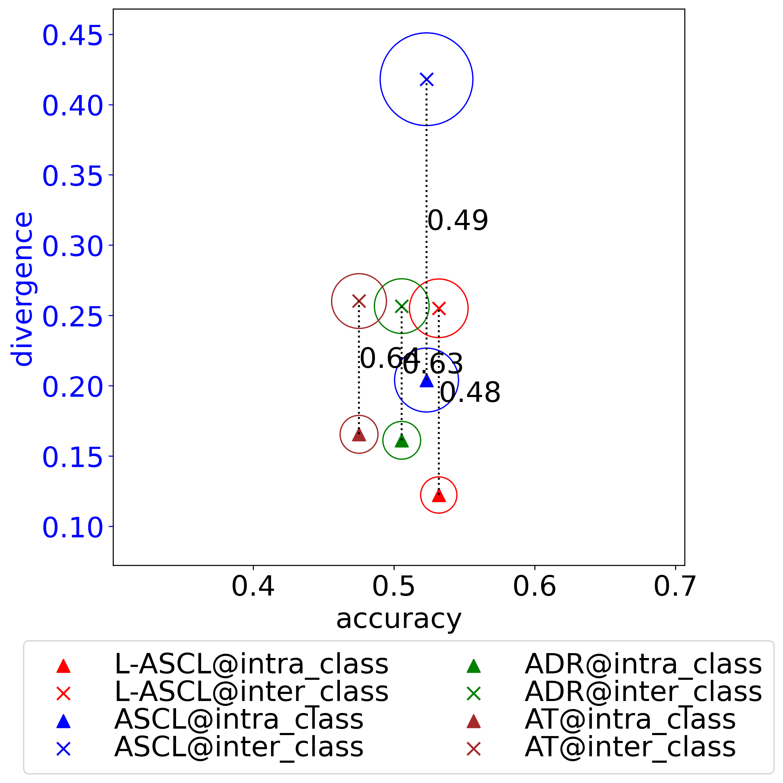
Figure 6: Pairs of Absolute-DIV with corresponding robust accuracy and R-DIV (noted in each line).

t-SNE visualization.

In addition to the quantitative evaluation as provided in Section 4.4 in the main paper, we provide a qualitative comparison via the t-SNE visualization as shown in Figure 7. The experiments have been conducted on the CIFAR10 dataset with ResNet20 architecture under PGD attack $\{\epsilon=8/255,\eta=2/255,k=250\}$. We visualize latent representations of 100 adversarial examples in addition to 1000 natural samples of the CIFAR10 dataset. It can be seen that: (i) In the NAT model as Figure 7a, the latent representations of natural images are well separate, which explains the high natural accuracy. However, the adversarial examples also are well separate and lay on the high confident area of each class (low entropy). It indicates that, adversarial examples fool the natural model easily with very high confident. (ii) In the AT model as Figure 7b, the latent representations of natural images are less detached, which explains the lower natural accuracy than the NAT model. The adversarial examples distribute randomly inside each cluster. The predictions of natural images and adversarial examples have higher entropy which means that the model is less confident. (iii) In our ASCL and Leaked-ASCL as Figure 7c, 7d, the latent representations of natural images are better distinguishable among classes. More specifically, the adversarial examples’ representations lay in the boundary of each cluster, which has higher entropy than those of natural images.

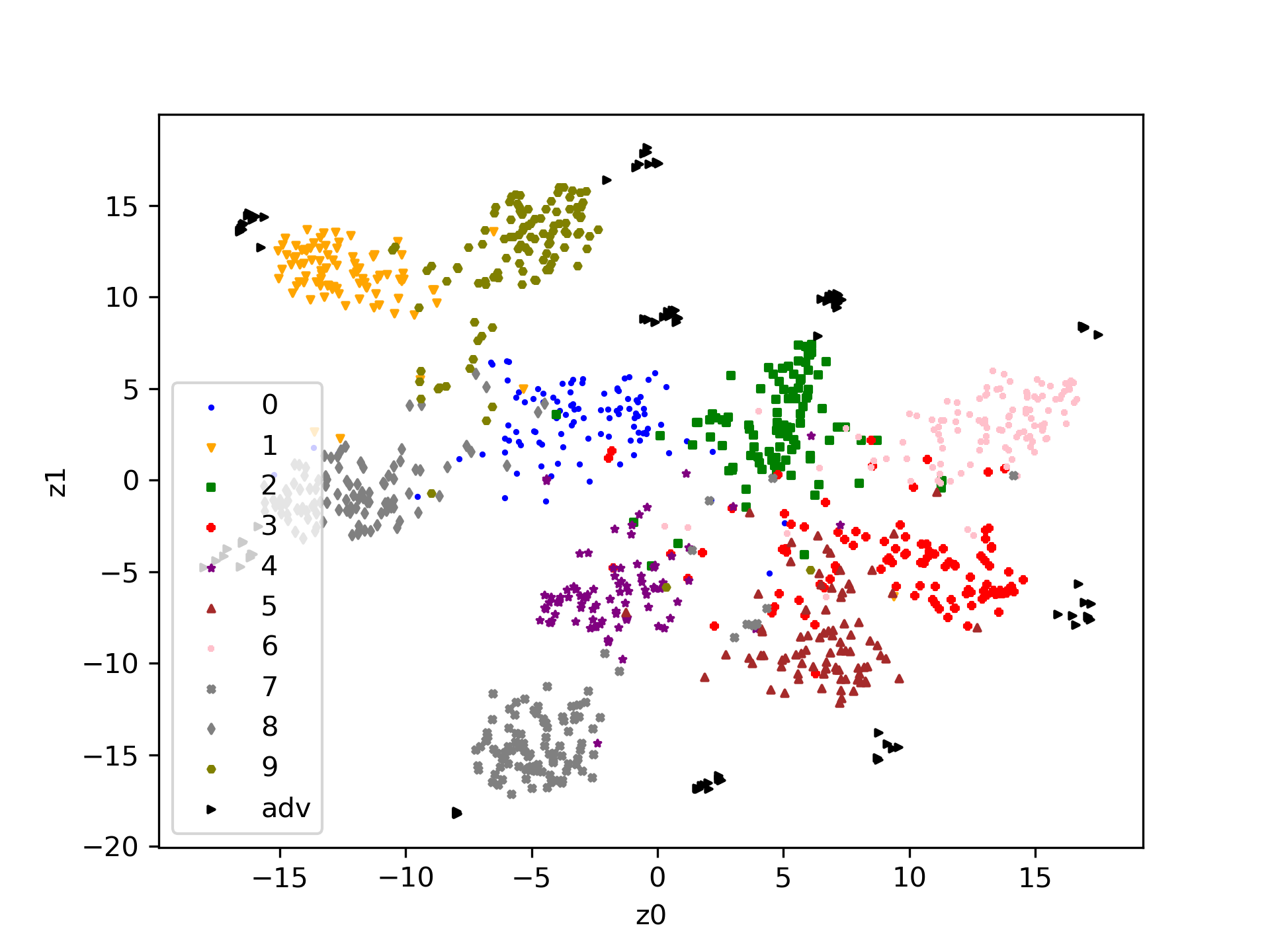
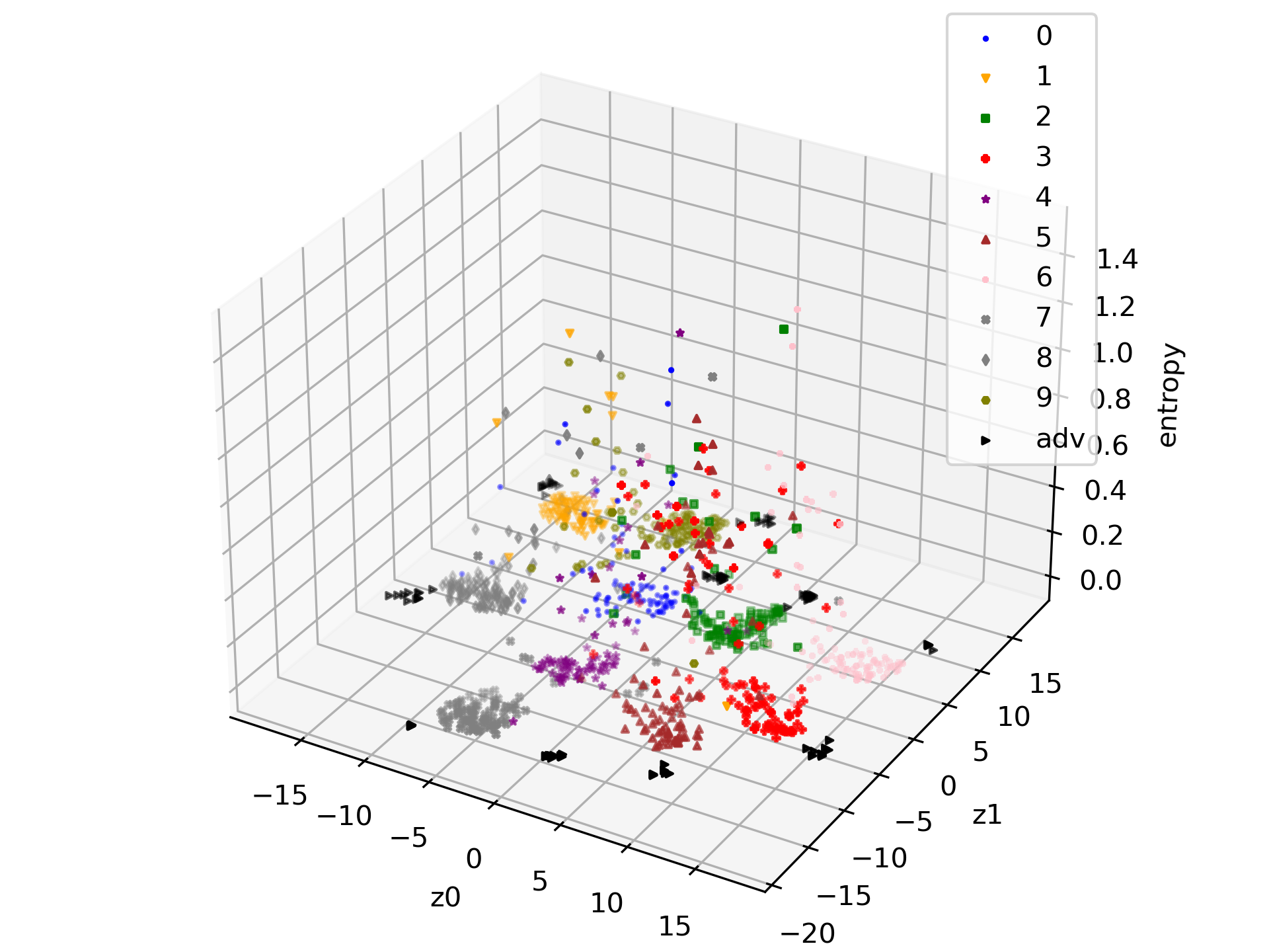
(a) NAT

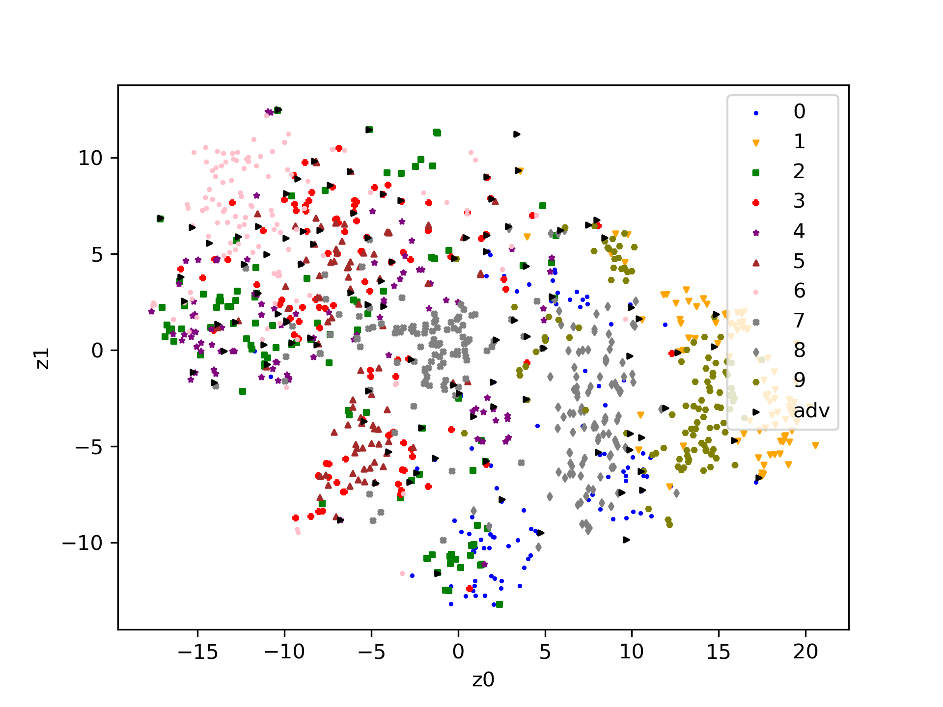
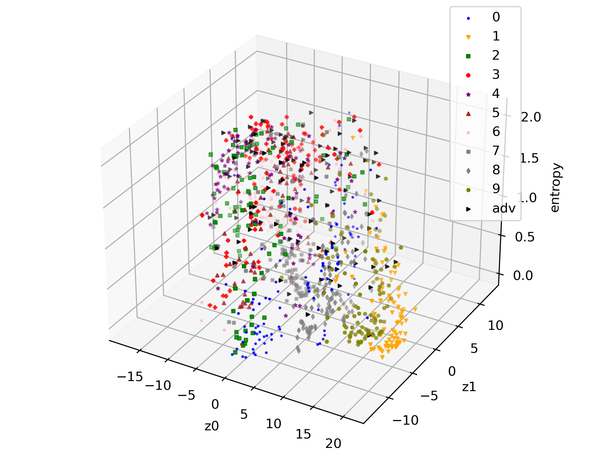
(b) AT

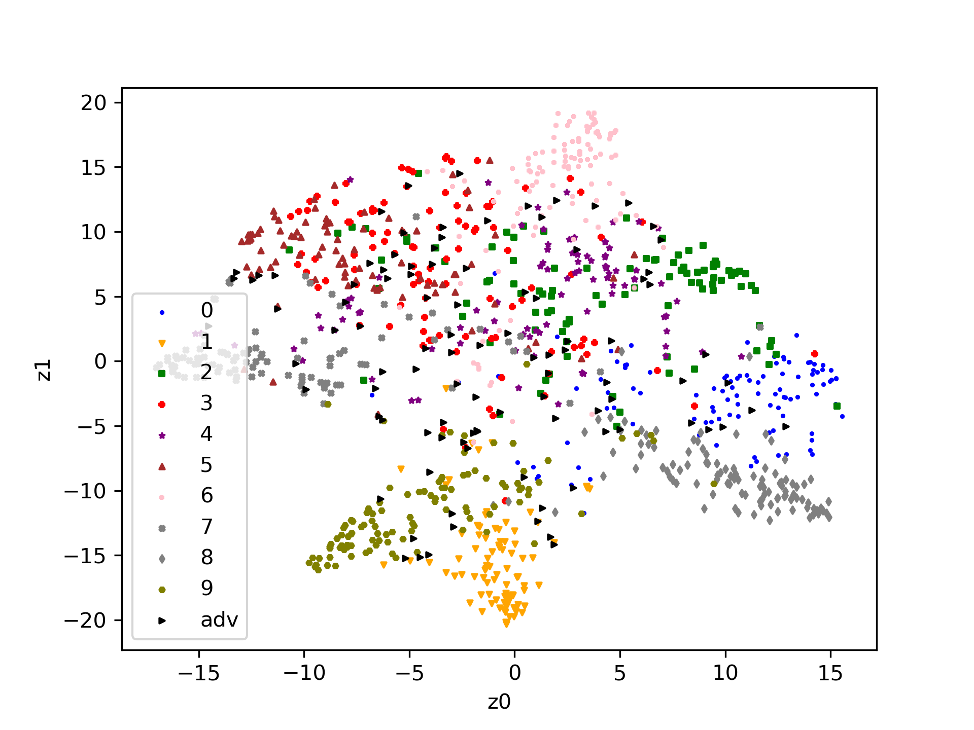
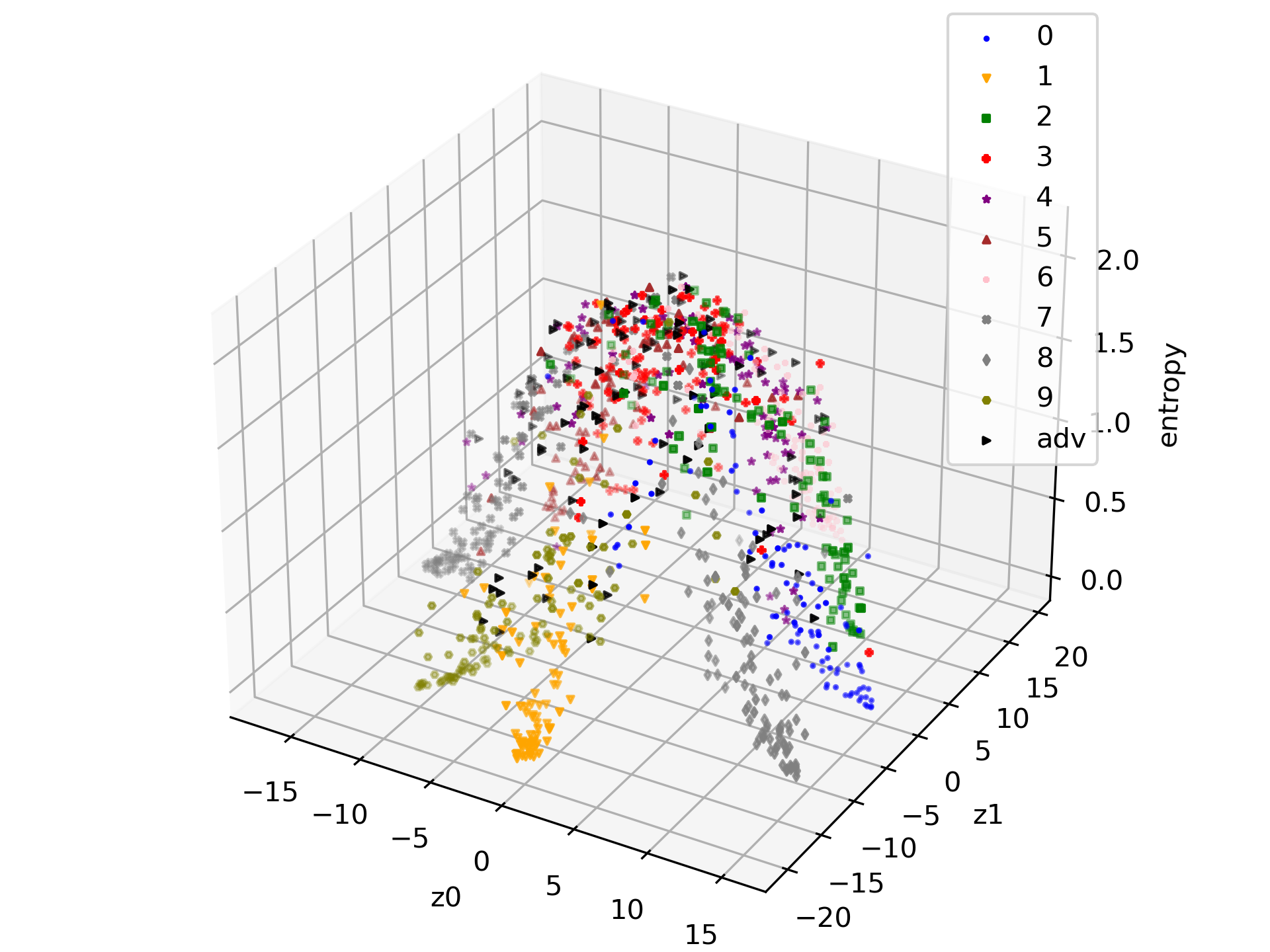
(c) ASCL

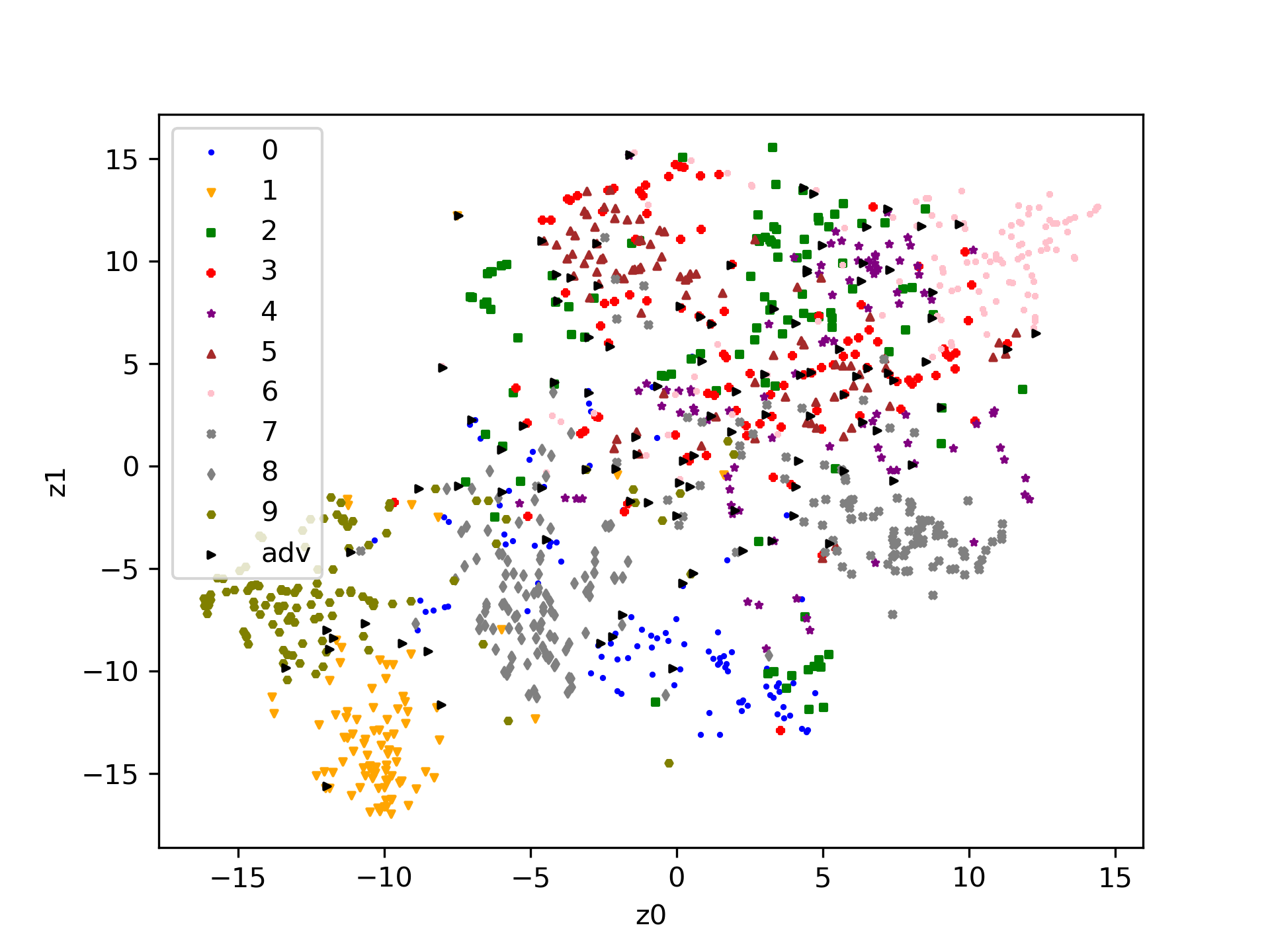
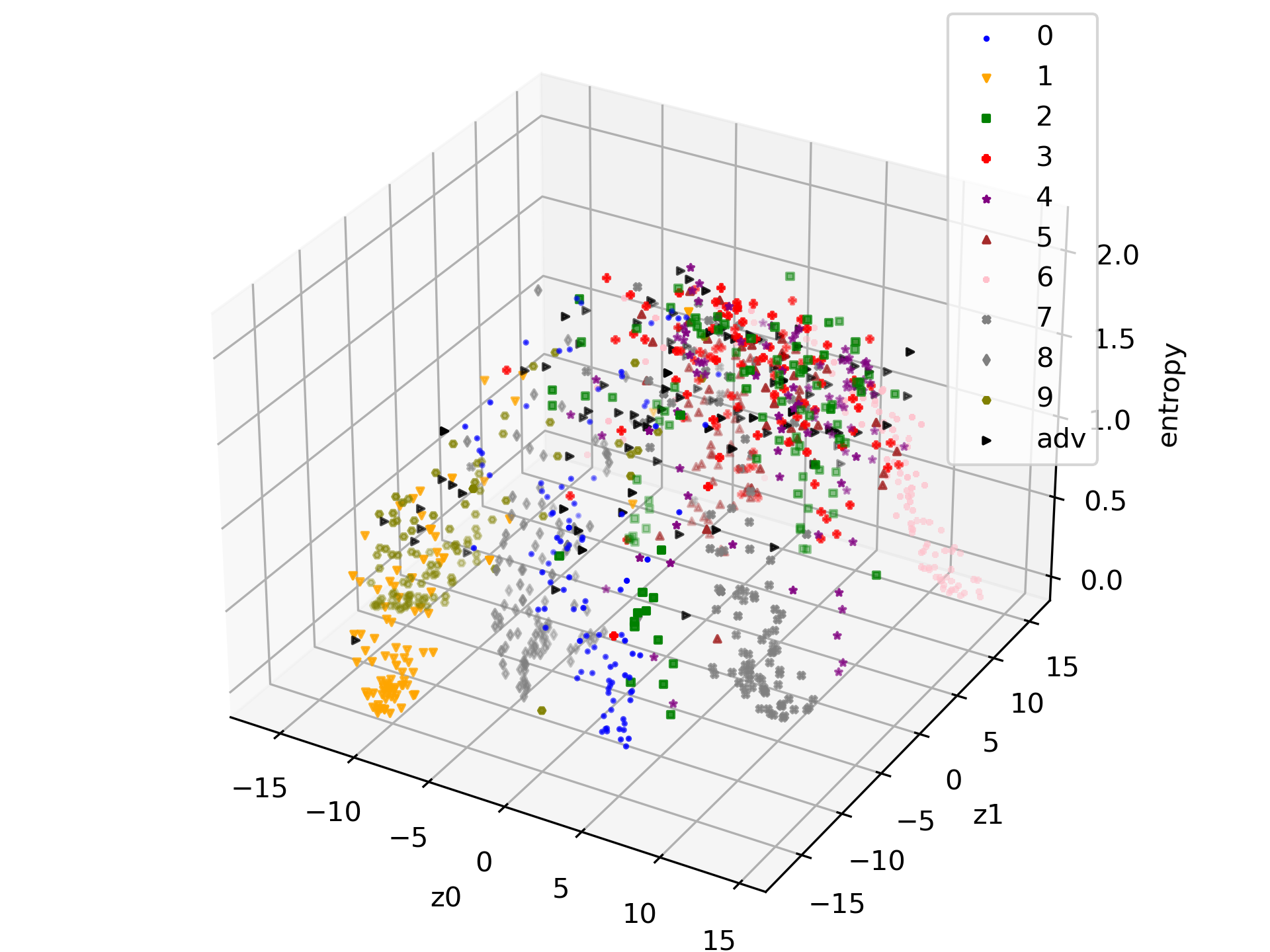
(d) Leaked-ASCL

Figure 7: t-SNE visualization of the latent space. Experiment on the CIFAR10 dataset with ResNet20 architecture. In each subfigure, the black-triangles represents for the adversarial examples. The left-subfigure is 2D t-SNE visualization while the right-subfigure is 2D t-SNE with entropy of prediction in the z-axis.

8 Additional Experimental Results

8.1 Projection Head in the context of AML

In this section we provide an additional ablation study to further understand the effect of the projection head in the context of AML. We apply our methods (ASCL and Leaked ASCL) with three options of the projection head as shown in Figure 8:

• A projection head with only single linear layer $\tilde{\mathbf{z}}=p^{1}(\mathbf{z})=W^{1}(\mathbf{z})$ with layer weight $W^{1}\in\mathcal{R}^{h\times\tilde{h}}$, where $h(\tilde{h})$ is the dimensionality of latent $\mathbf{z}(\tilde{\mathbf{z}})$. We choose $\tilde{h}=128$ in our experiments.

• A projection head with two fully connected layers without bias $\tilde{\mathbf{z}}=p^{2}(\mathbf{z})=W^{2}\left(Relu(W^{1}(\mathbf{z})\right)$ with layer weight $W^{1}\in\mathcal{R}^{h\times 200}$ and $W^{2}\in\mathcal{R}^{200\times 128}$ and

• Identity mapping $\tilde{\mathbf{z}}=\mathbf{z}$.

Table 5 shows the performances of three options on the CIFAR10 dataset with ResNet20 architecture. We observe that the linear projection head $p^{1}()$ is better than the identity mapping on both natural accuracy (by around 1%) and robust accuracy (on average 0.7%). In contrast, the non-linear projection head $p^{2}()$ reduces the robust accuracy on average 0.5%.

The improvement on the natural accuracy concurs with the finding in Chen et al., (2020) which can be explained by the fact that the projection head helps to reduce the dimensionality to apply the contrastive loss more efficiently. As shown in Section B.4 in Chen et al., (2020) that even using the same output size, the weight of the projection head has relatively few large eigenvalues, indicating that it is approximately low-rank.

On the other hand, the effect of the projection head to the robust accuracy is due to its non-linearity. Figure 8a demonstrates the training flow and attack flow on our framework with the projection head. The contrastive loss $\mathcal{L}^{SCL}$ is applied in the projected layer $\tilde{\mathbf{z}}$ which induces the compactness on the projected layer but not the intermediate layer $\mathbf{z}$. Therefore, when using a non-linear projection head (e.g., $p^{2}$), the compactness in the intermediate layer is weaker than the projected layer. For example, a relationship $\left\|\tilde{\mathbf{z}}_{i}-\tilde{\mathbf{z}}_{j}\right\|_{p}\leq\left\|\tilde{\mathbf{z}}_{i}-\tilde{\mathbf{z}}_{k}\right\|_{p}$ in the projected layer can not imply a relationship $\left\|\mathbf{z}_{i}-\mathbf{z}_{j}\right\|_{p}\leq\left\|\mathbf{z}_{i}-\mathbf{z}_{k}\right\|_{p}$ in the intermediate layer. It explains why using the non-linear projection head reduces the effectiveness of the SCL to the adversarial robustness.

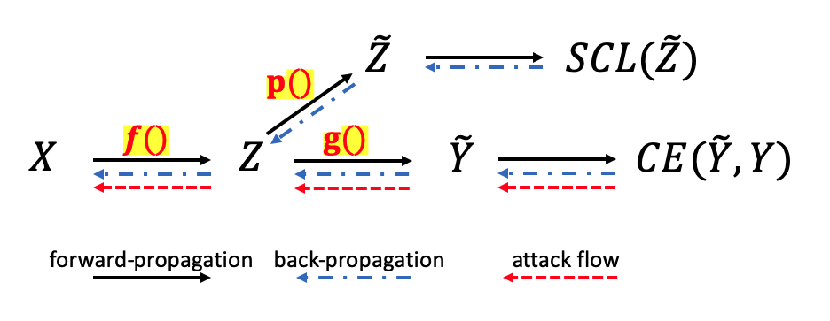
(a) with the projection head

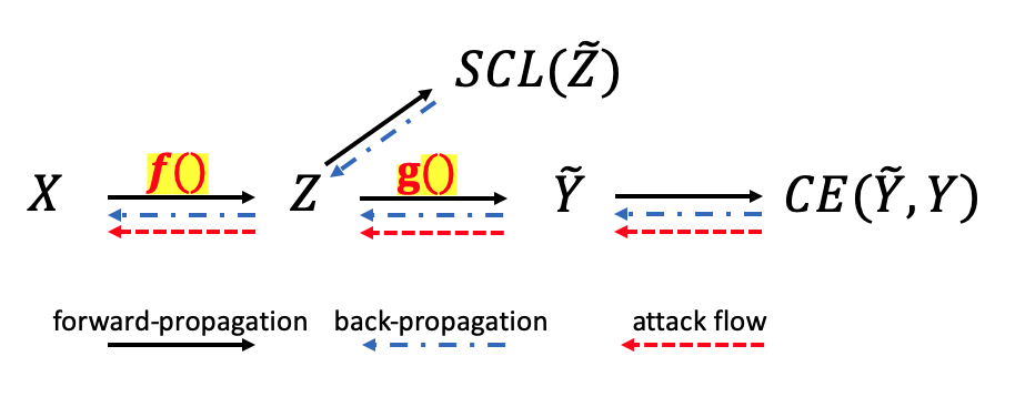
(b) without the projection head

Figure 8: Training/Attack flows with/without the projection head

Table 5: Performance comparison with/without the projection head $p()$ on the CIFAR10 dataset with ResNet20 architecture. $p^{1}()$ and $p^{2}()$ represent for the projection head with one layer and two layers respectively.

	Nat.	PGD	AA
ASCL without $p()$	76.4	52.7	40.9
ASCL with $p^{1}()$	77.3	53.3	41.3
ASCL with $p^{2}()$	76.6	52.3	39.7
(Leaked)ASCL without $p()$	75.5	53.7	42.0
(Leaked)ASCL with $p^{1}()$	76.5	54.1	42.3
(Leaked)ASCL with $p^{2}()$	75.7	52.9	41.1

8.2 Contribution of each component in ASCL

We provide an ablation study to investigate the contribution of each of ASCL’s components to the performance and emphasize the importance of our SCL component. We experiment on the CIFAR10 dataset with two architectures, i.e., ResNet18 and WideResNet-34-10 (WRN). There are two remarks that can be observed from Table 6 such that:

(i) Using original SCL slightly improves the adversarial robustness against weak adversarial attacks but cannot defend strong ones. More specifically, the robust accuracy against PGD with $\epsilon=8/255,k=5,\eta=2/255$ is $1.2\%$ while that for non-defence model is $0.0\%$. However, the robust accuracy drops to $0.0\%$ against stronger attacks, i.e., PGD with $\epsilon=8/255,k=250,\eta=2/255$ or Auto-Attack. A similar observation was observed in Kim et al., (2020) when the original SCL only achieves $0.08\%$ robust accuracy. The result shows that while the original contrastive learning induces weak robustness in DNN models as our analysis in Section 2, directly adopting contrastive learning into AML hardly improves the adversarial robustness against strong attacks which emphasizes the importance of our adaptions.

(ii) Adding SCL significantly improves the natural performance and adversarial robustness of the model. More specifically, with ResNet18 architecture, adding SCL to ADV can gain improvements of $2.3\%$ of natural accuracy and $1.5\%$ of robust accuracy against Auto-Attack. With WideResNet architecture, the improvements of natural/robust accuracies are $2.7\%$ and $1.7\%$, respectively. Similar improvements can be observed when adding SCL to ADV+VAT. More specifically, the gaps of natural accuracy with/without SCL are $0.8\%$ and $1.1\%$ in experiments with ResNet18 and WideResNet, respectively. These gaps of robust accuracy against Auto-Attack are $0.3\%$ and $0.7\%$.

Table 6: Ablation study on the CIFAR10 dataset with different architectures. orgSCL represents the original SCL version with two standard data-augmentations. Bold numbers indicate there are improvements over the previous settings (i.e., only using ADV or using both ADV and VAT) when adding our SCL.

	Model	Nat.	PGD	AA
orgSCL	ResNet18	93.80	0.0	0.0
ADV	ResNet18	82.75	52.95	48.81
ADV+SCL	ResNet18	85.02	53.40	50.31
ADV+VAT	ResNet18	83.73	53.00	49.39
ADV+VAT+SCL	ResNet18	84.54	54.29	49.66
ADV	WRN	84.93	55.04	51.12
ADV+SCL	WRN	87.70	54.05	52.80
ADV+VAT	WRN	85.96	54.76	51.87
ADV+VAT+SCL	WRN	87.12	55.93	52.53

We provide an additional experiment to further understand the contribution of each component in our framework. Table 7 shows the result on the CIFAR10 dataset with ResNet20 architecture. We observe that using SCL alone can helps to improve the natural accuracy, but enforcing the contrastive loss too much reduces the effectiveness. On the other hand, increasing the VAT’s weight increases the robustness but significantly reduces the natural performance which concurs with the finding in Zhang et al., (2019). Therefore, to balance the trade-off between natural accuracy and robustness, we choose $\lambda^{SCL}=1,\lambda^{VAT}=2$ as the default setting in our framework.

Table 7: Ablation study with different parameter settings on the CIFAR10 dataset with ResNet20.

	Nat.	PGD	AA
$\lambda^{SCL}=0,\lambda^{VAT}=0$	78.8	48.1	36.1
$\lambda^{SCL}=1,\lambda^{VAT}=0$	80.1	46.5	34.7
$\lambda^{SCL}=2,\lambda^{VAT}=0$	79.5	46.7	34.7
$\lambda^{SCL}=3,\lambda^{VAT}=0$	79.6	45.8	34.4
$\lambda^{SCL}=4,\lambda^{VAT}=0$	79.2	45.6	34.3
$\lambda^{SCL}=0,\lambda^{VAT}=1$	77.4	50.6	38.2
$\lambda^{SCL}=0,\lambda^{VAT}=2$	75.4	53.0	40.0
$\lambda^{SCL}=0,\lambda^{VAT}=3$	73.3	54.4	42.3
$\lambda^{SCL}=0,\lambda^{VAT}=4$	71.2	55.0	43.1

8.3 Global and Local Selections

We provide an example of selected positive and negative samples which have been chosen by the Leaked-Local Selection as Figure 9. It can be seen that, with the same query image, the corresponding negatives and positives have been selected differently overtime. More specifically, at the beginning of training progress (epoch 1, Figure 9a), only few positive images (2-4 images) were picked, while those of negatives are larger (around 14-16 images). Correlating with the model performance, the number of positive images increases while the number of negative images decreases. At the end of training progress (epoch 200, Figure 9c) there are 8 natural images and 3 adversarial images in the positive set, while those in the negative set are 2 natural images and 3 adversarial images. The changing of positives/negatives in this example is inline with the statistic as in Figure 3b in the main paper. In addition, given an anchor image $\mathbf{x}_{i}$ , the natural image $\mathbf{x}_{j}$ and adversarial image $\mathbf{x}_{j}^{a}$ ($j\neq i$) have been treated independently as in Table 1 in the main paper, therefore, we get more flexible in the positive and negative set, for example, only one of $\mathbf{x}_{j}$ or $\mathbf{x}_{j}^{a}$ has been selected as a negative (or a positive) as in Figure 9.

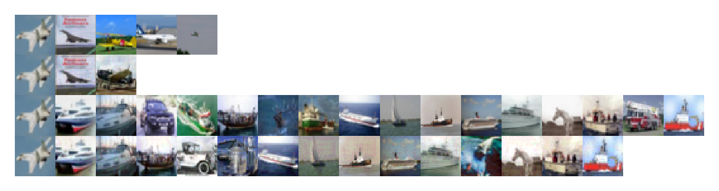
(a) Epoch 1

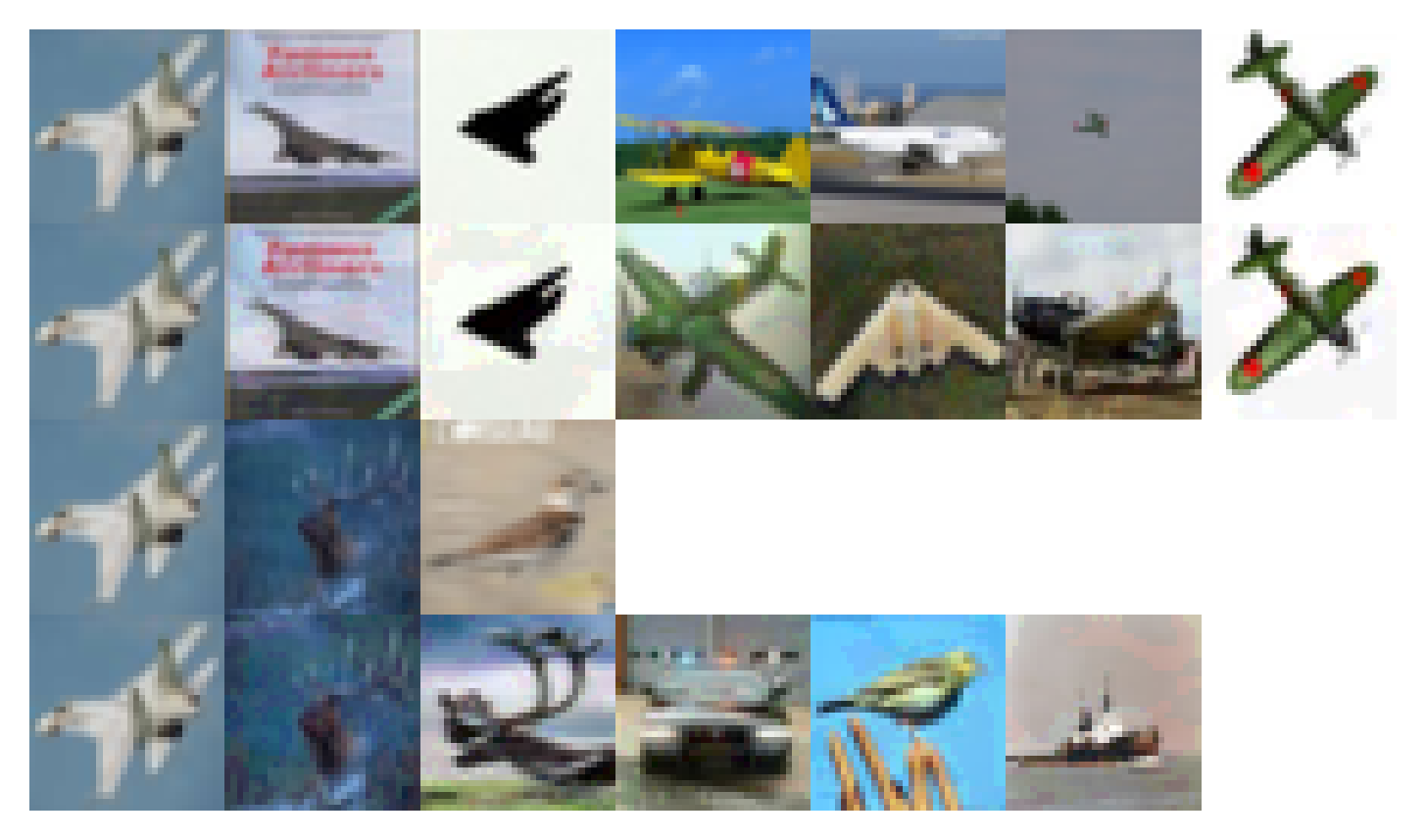
(b) Epoch 30

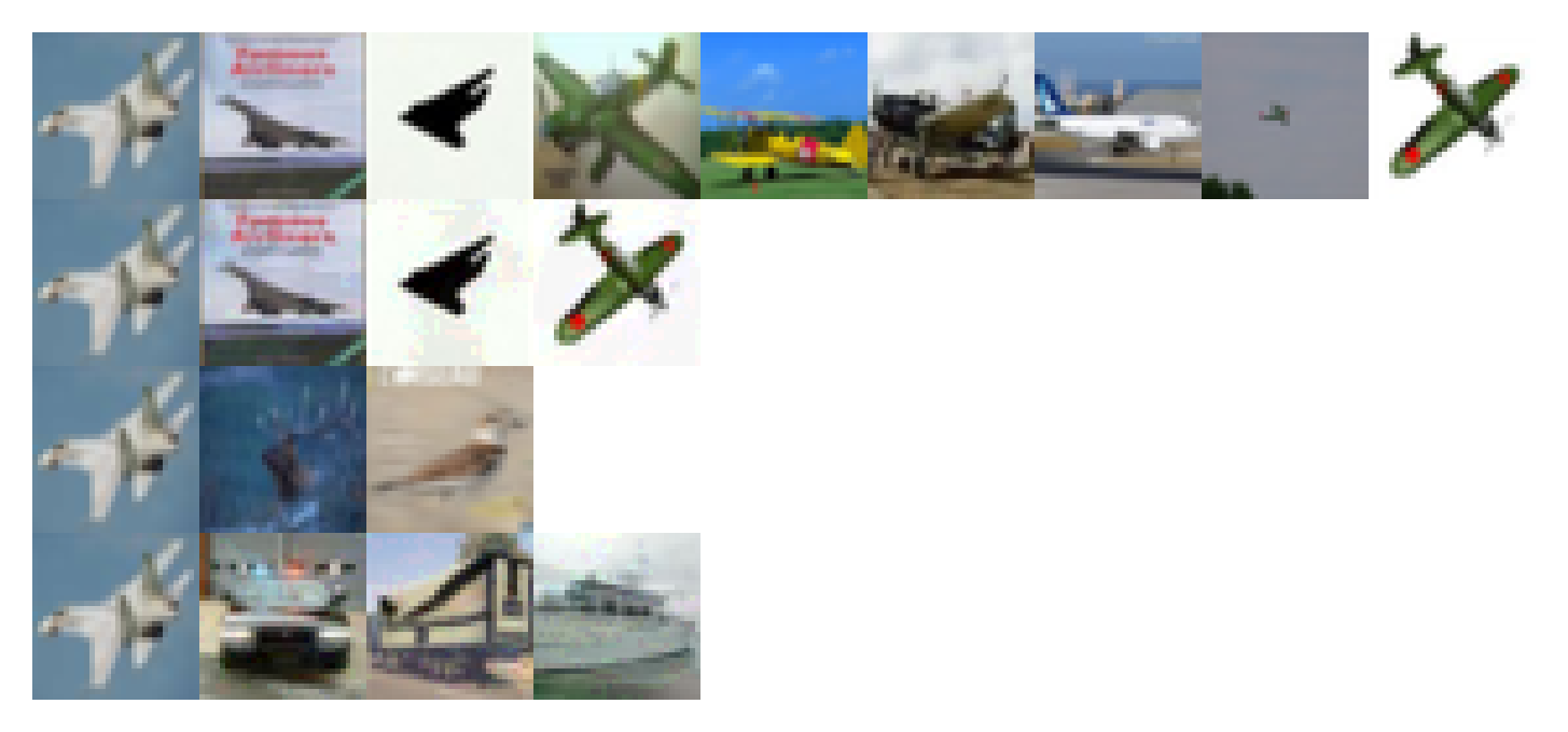
(c) Epoch 200

Figure 9: Positive and negative samples from the Leaked Local Selection strategy. In each image, the first column represents the anchor followed by its positive and negative samples. Row 1 and 2 represent the natural and adversarial positive samples respectively. Row 3 and 4 represent the natural and adversarial negative samples respectively.

9 Background and Related works

In this section, we present a fundamental background and related works to our approach. First, we introduce well-known contrastive learning frameworks, followed by a brief introduction of adversarial attack and defense methods. We then provide a comparison of our approach with defense methods on a latent space, especially, those integrated with contrastive learning frameworks.

9.1 Contrastive Learning

9.1.1 General formulation

Self-Supervised Learning (SSL) became an important tool that helps Deep Neural Networks exploit structure from gigantic unlabeled data and transfers it to downstream tasks. The key success factor of SSL is choosing a pretext task that heuristically introduces interaction among different parts of the data (e.g., CBOW and Skip-gram Mikolov et al., (2013), predicting rotation Gidaris et al., (2018)). Recently, Self-Supervised Contrastive Learning (SSCL) with contrastive learning as the pretext task surpasses other SSL frameworks and nearly achieves supervised-learning’s performance. The main principle of SSCL is to introduce a contrastive correlation among visual representations of positives (’similar’) and negatives (’dissimilar’) with respect to an anchor one. There are several SSCL frameworks have been proposed (e.g., MoCo He et al., (2020), BYOL Grill et al., (2020), CURL Srinivas et al., (2020)), however, in this section, we mainly introduce the SSCL in Chen et al., (2020) which had been integrated with adversarial examples to improve adversarial robustness in Kim et al., (2020); Jiang et al., (2020) followed by the Supervised Contrastive Learning (SCL) Khosla et al., (2020) which has been used in our approach.

Consider a batch of N pairs $\{\mathbf{x}_{i},\boldsymbol{y}_{i}\}_{i=1}^{N}$ of benign images and their labels. With two random transformations $\mathcal{T},\mathcal{A}$ we have a set of transformed images $\{\mathbf{x}_{i}^{\mathcal{T}},\mathbf{x}_{i}^{\mathcal{A}},\boldsymbol{y}_{i}\}_{i=1}^{N}$. The general formulation of contrastive learning as follow:

$$\mathcal{L}^{\text{CL}}=\frac{1}{N}\sum_{i=1}^{N}\mathcal{L}_{i}^{\mathcal{T},cl}+\mathcal{L}_{i}^{\mathcal{A},cl}$$ (7)

where $\mathcal{L}_{i}^{\mathcal{T}.cl}$ is the contrastive loss w.r.t. the anchor $\mathbf{x}_{i}^{\mathcal{T}}$:

$$\mathcal{L}_{i}^{\mathcal{T},cl}=\frac{-1}{\left|\boldsymbol{Z}_{i}^{+}\right|+1}\underset{\mathbf{z}_{j}\in\boldsymbol{Z}_{i}^{+}\cup\{\mathbf{z}_{i}^{\mathcal{A}}\}}{\sum}\log\frac{e^{\frac{sim(\mathbf{z}_{j},\mathbf{z}_{i}^{\mathcal{T}})}{\tau}}}{\underset{\mathbf{z}_{k}\in\boldsymbol{Z}_{i}^{+}\cup\boldsymbol{Z}_{i}^{-}\cup\{\mathbf{z}_{i}^{\mathcal{A}}\}}{\sum}e^{\frac{sim(\mathbf{z}_{k},\mathbf{z}_{i}^{\mathcal{T}})}{\tau}}}$$ (8)

and $\mathcal{L}_{i}^{\mathcal{A},cl}$ is the contrastive loss w.r.t. the anchor $\mathbf{x}_{i}^{\mathcal{A}}$:

$$\mathcal{L}_{i}^{\mathcal{A},cl}=\frac{-1}{\left|\boldsymbol{Z}_{i}^{+}\right|+1}\underset{\mathbf{z}_{j}\in\boldsymbol{Z}_{i}^{+}\cup\{\mathbf{z}_{i}^{\mathcal{T}}\}}{\sum}\log\frac{e^{\frac{sim(\mathbf{z}_{j},\mathbf{z}_{i}^{\mathcal{A}})}{\tau}}}{\underset{\mathbf{z}_{k}\in\boldsymbol{Z}_{i}^{+}\cup\boldsymbol{Z}_{i}^{-}\cup\{\mathbf{z}_{i}^{\mathcal{T}}\}}{\sum}e^{\frac{sim(\mathbf{z}_{k},\mathbf{z}_{i}^{\mathcal{A}})}{\tau}}}$$ (9)

The formulation shows the general principle of contrastive learning such that: (i) $\boldsymbol{Z}_{i}^{+}\cup\boldsymbol{Z}_{i}^{-}\cup\{\mathbf{z}_{i}^{\mathcal{A}},\mathbf{z}_{i}^{\mathcal{T}}\}=\{\mathbf{z}_{j}^{\mathcal{T}},\mathbf{z}_{j}^{\mathcal{A}}\}_{j=1}^{N}\;\forall i\in[1,N]$ where $\boldsymbol{Z}_{i}^{+}$ and $\boldsymbol{Z}_{i}^{-}$ are positive and negative sets which are defined differently depending on self-supervised/supervised setting, (ii) without loss of generality, in Equation 8, the similarity $e^{\frac{sim(\mathbf{z}_{j},\mathbf{z}_{i}^{\mathcal{T}})}{\tau}}$ between the anchor $\mathbf{z}_{i}^{\mathcal{T}}$ and a positive sample $\mathbf{z}_{j}\in\boldsymbol{Z}_{i}^{+}\cup\{\mathbf{z}_{i}^{\mathcal{A}}\}$ has been normalized with sum of all possible pairs between the anchor and the union set of $\boldsymbol{Z}_{i}^{+}\cup\boldsymbol{Z}_{i}^{-}\cup\{\mathbf{z}_{i}^{\mathcal{A}}\}$ to ensures that the log argument is not higher than 1, (iii) the contrastive loss in Equation 8 pulls anchor representation $\mathbf{z}_{i}^{\mathcal{T}}$ and the positives’ representations $\boldsymbol{Z}_{i}^{+}\cup\{\mathbf{z}_{i}^{\mathcal{A}}\}$ close together while pushes apart those of negatives $\boldsymbol{Z}_{i}^{-}$.

Explanation for our Formulation.

It is worth noting that, our derivation shows the general formulation of the contrastive learning which can be adapted to SSCL Chen et al., (2020), SCL Khosla et al., (2020) or our Local ASCL by defining the positive and negative sets differently. Moreover, by using terminologies positive set $\boldsymbol{Z}_{i}^{+}$ and those sample from the same instance $\{\mathbf{z}_{i}^{\mathcal{T}},\mathbf{z}_{i}^{\mathcal{A}}\}$ separately, we emphasize the importance of the anchor’s transformation which stand out other positives. Last but not least, our derivation normalizes the contrastive loss in Equation 7 to the same scale with the cross-entropy loss and the VAT loss as in Section 3, which helps to put all terms together appropriately.

Self-Supervised Contrastive Learning.

In SSCLChen et al., (2020), the positive set (excluding those samples from the same instance $\mathbf{z}_{i}^{\mathcal{A}},\mathbf{z}_{i}^{\mathcal{T}}$) $\boldsymbol{Z}_{i}^{+}=\emptyset$ $(\left|\boldsymbol{Z}_{i}^{+}\right|=0)$ while the negative set $\boldsymbol{Z}_{i}^{-}=\{\mathbf{z}_{j}^{\mathcal{T}},\mathbf{z}_{j}^{\mathcal{A}}\mid j\neq i\}$ which includes all other samples except those from the same instance $\mathbf{z}_{i}^{\mathcal{A}},\mathbf{z}_{i}^{\mathcal{T}}$. In this case, the formulation of SSCL as follow:

$$\mathcal{L}_{i}^{\mathcal{T},sscl}=-\log\frac{e^{\frac{sim(\mathbf{z}_{j},\mathbf{z}_{i}^{\mathcal{T}})}{\tau}}}{\underset{\mathbf{z}_{k}\in\boldsymbol{Z}_{i}^{-}\cup\{\mathbf{z}_{i}^{\mathcal{A}}\}}{\sum}e^{\frac{sim(\mathbf{z}_{k},\mathbf{z}_{i}^{\mathcal{T}})}{\tau}}}$$ (10)

and

$$\mathcal{L}_{i}^{\mathcal{A},sscl}=-\log\frac{e^{\frac{sim(\mathbf{z}_{j},\mathbf{z}_{i}^{\mathcal{A}})}{\tau}}}{\underset{\mathbf{z}_{k}\in\boldsymbol{Z}_{i}^{-}\cup\{\mathbf{z}_{i}^{\mathcal{T}}\}}{\sum}e^{\frac{sim(\mathbf{z}_{k},\mathbf{z}_{i}^{\mathcal{A}})}{\tau}}}$$ (11)

Supervised Contrastive Learning.

The SCL framework leverages the idea of contrastive learning with the presence of label supervision to improve the regular cross-entropy loss. The positive set and the negative set are $\boldsymbol{Z}_{i}^{+}=\{\mathbf{z}_{j}^{\mathcal{T}},\mathbf{z}_{j}^{\mathcal{A}}\mid j\neq i,\boldsymbol{y}_{j}=\boldsymbol{y}_{i}\}$ and $\boldsymbol{Z}_{i}^{-}=\{\mathbf{z}_{j}^{\mathcal{T}},\mathbf{z}_{j}^{\mathcal{A}}\mid j\neq i,\boldsymbol{y}_{j}\neq\boldsymbol{y}_{i}\}$, respectively. As mentioned in Khosla et al., (2020), there is a major advantage of SCL compared with SSCL in the context of regular machine learning. Unlike SSCL in which each anchor has only single positive sample, SCL takes advantages of the labels to have many positives in the same batch size N. This strategy helps to reduce the false negative cases in SSCL when two samples in the same class are pushed apart. As shown in Khosla et al., (2020), the SCL training is more stable than SSCL and also achieves a better performance.

9.1.2 Important factors for Contrastive Learning

Data augmentation.

Chen et al. Chen et al., (2020) empirically found that SSCL needs stronger data augmentation than supervised learning. While the SSCL’s performance experienced a huge gap of 5% with different data augmentation (Table 1 in Chen et al., (2020)), the supervised performance was not changed much with the same set of augmentation. Therefore, in our paper, to reduce the space of hyper-parameters we use only one adversarial transformation $\mathcal{A}$(e.g., PGDMadry et al., (2018) or TRADESZhang et al., (2019)) while using the identity transformation $\mathcal{T}$, $\mathbf{x}_{i}^{\mathcal{T}}=\mathbf{x}_{i}$ ($\mathbf{z}_{i}^{\mathcal{T}}=\mathbf{z}_{i}$), and let the investigation of using different data augmentations for future works.

Batch size.

As shown in Figure 9 in Chen et al., (2020), the batch size is an important factor that strongly affects the performance of the contrastive learning framework. A larger batch size comes with larger positive and negative sets, which helps to generalize the contrastive correlation better and therefore improves the performance. He et al. He et al., (2020) proposed a memory bank to store the previous batch information which can lessen the batch size issue. In our framework, because of the limitation on computational resources, we only tried with a small batch size (128) which likely limits the contribution of our methods.

Projection head.

Normally, the representation vector which is the output of the encoder network has very high dimensionality, e.g., the final pooling layer in ResNet-50 and ResNet-200 has 2048 dimensions. Therefore, applying contrastive learning directly on this intermediate layer is less effective. Alternatively, CL frameworks usually use a projection network $p()$ to project the normalized representation vector $\mathbf{z}$ into a lower dimensional vector $\tilde{\mathbf{z}}=p(\mathbf{z})$ which is more suitable for computing the contrastive loss. To avoid over-parameterized, CL frameworks usually choose a small projection head with only one or two fully-connected layers.

9.2 Adversarial attack

Projected Gradient Decent (PGD).

is an iterative version of the FGSM attack Goodfellow et al., (2015) with random initialization Madry et al., (2018). It first randomly initializes an adversarial example in a perturbation ball by adding uniform noise to a clean image, followed by multiple steps of one-step gradient ascent, at each step projecting onto the perturbation ball. The formula for the one-step update is as follows:

$$x_{a}^{t+1}=\text{Proj${}_{B_{\varepsilon}\left(x\right)}$}(x_{a}^{t}+\eta\;\text{sign}\left(\nabla\ell(x,y,\theta)\right)$$ (12)

where $B_{\varepsilon}\left(x\right)\triangleq\left\{x^{\prime}:\left\|x^{\prime}-x\right\|<\varepsilon\right\}$ is the perturbation ball with radius $\varepsilon$ around $x$and $\eta$ is the gradient scale for each step update.

Auto-Attack.

Even the most popular attack, PGD can still fail in some extreme cases Croce et al., (2019) because of two issues: (i) fixed step size $\eta$ which leads to sub-optimal solutions and (ii) the sensitivity of a gradient to the scale of logits in the standard cross-entropy loss. Auto-Attack Croce and Hein, (2020) proposed two variants of PGD to deal with these potential issues by (i) automatically selecting the step size across iterations (ii) an alternative logit loss which is both shift and rescaling invariant. Moreover, to increase the diversity among the attacks used, Auto-Attack combines two new versions of PGD with the white-box attack FAB Croce and Hein, (2019)and the blackbox attack Square Attack Andriushchenko et al., (2020) to form a parameter-free, computationally affordable, and user-independent ensemble of complementary attacks to estimate adversarial robustness. Therefore, besides PGD, Auto-Attack is considered as the new standard evaluation for adversarial robustness.

9.3 Adversarial defense

9.3.1 Adversarial training

Adversarial training (AT) originate in Goodfellow et al., (2015), which proposed incorporating a model’s adversarial examples into training data to make the model’s loss surface to be smoother, thus, improve its robustness. Despite its simplicity, AT Madry et al., (2018) was among the few that were resilient against attacks other than gave a false sense of robustness because of the obfuscated gradient Athalye et al., (2018). To continue its success, many AT’s variants have been proposed including (1) different types of adversarial examples (e.g., the worst-case examples Goodfellow et al., (2015) or most divergent examples Zhang et al., (2019)), (2) different searching strategies (e.g., non-iterative FGSM, Rand FGSM with a random initial point or PGD with multiple iterative gradient descent steps Madry et al., (2018)), (3) additional regularizations, e.g., adding constraints in the latent space Zhang and Wang, (2019); Bui et al., (2020), (4) difference in model architecture, e.g., activation function Xie et al., (2020) or ensemble models Pang et al., (2019).

9.3.2 Defense with a latent space

Unlike an input space $\boldsymbol{X}$, a latent space $\boldsymbol{Z}$ has a lower dimensionality and a higher mutual information with the prediction space than the input one $I(Z,Y)\geq I(X,Y)$ Tishby and Zaslavsky, (2015). Therefore, defense with the latent space has particular characteristics to deal with adversarial attacks notably Zhang and Wang, (2019); Bui et al., (2020); Mao et al., (2019); Xie et al., (2019); Samangouei et al., (2018). For example, DefenseGAN Samangouei et al., (2018) used a pretrained GAN which emulates the data distribution to generate a denoised version of an adversarial example. On the other hand, instead of removing noise in the input image, Xie et al. Xie et al., (2019) attempted to remove noise in the feature space by using non-local means as a denoising block. However, these works were criticized by Athalye et al., (2018) as being easy to attack by approximating the backward gradient signal.

9.3.3 Defense with contrastive learning

The idea of defense with contrastive correlation in the latent space can be traced back to Mao et al., (2019) which proposed an additional triplet regularization to adversarial training. However, the triplet loss can only handle one positive and negative at a time, moreover, requires computationally expensive hard negative mining Schroff et al., (2015). As discussed in Khosla et al., (2020), the triplet loss is a special case of the contrastive loss when the number of positives and negatives are each one and has lower performance in general than the contrastive loss. Recently, Jiang et al., (2020); Kim et al., (2020) integrated SSCL Chen et al., (2020) to learn unsupervised robust representations for improving robustness in unsupervised/semi-supervised setting. Specifically, both methods proposed a new kind of adversarial examples which is based on the SSCL loss instead of regular cross-entropy loss Goodfellow et al., (2015) or KL divergence Zhang et al., (2019). By adversarially pre-training with these adversarial examples, the encoder is robust against the instance-wise attack and obtains comparable robustness to supervised adversarial training as reported in Kim et al., (2020). On the other hand, Jiang et al. Jiang et al., (2020) proposed three options of pre-training. However, their best method made use of two adversarial examples that requires a much higher computational cost to generate. Although these above works have the similar general idea of using contrastive learning to improve adversarial robustness with ours, we choose to compare our methods with RoCL-AT/TRADES in Kim et al., (2020) which is most close to our problem setting. More specifically, after pre-training phase with adversarial examples w.r.t. the contrastive loss, RoCL-AT/TRADES apply fine-tuning with standard supervised adversarial training, which requires full label. We use the reported result as in Table 1 in Kim et al., (2020) which used a larger batch size (256). It is a worth noting that the best reported version RoCL-AT-SS achieves 91.34% natural accuracy and 49.66% robust accuracy is a fine-tuned on a ImageNet pretrained model with self-supervised loss (e.g., SimCLR Chen et al., (2020)), therefore, is not as a reference for comparison.

Most closely related to our work is Bui et al., (2020) which also aims to realize the compactness in latent space to improve the robustness in supervised setting. They proposed a label weighting technique that sets the positive weight to the divergence of two examples in the same class and negative weight in any other cases. Therefore, when minimizing the divergence loss with label weighting, the divergences of those in the same class (positives) are encouraged to be close together, while those of different classes (negatives) to be distant.

References

- Akhtar and Mian, (2018) Akhtar, N. and Mian, A. (2018). Threat of adversarial attacks on deep learning in computer vision: A survey. IEEE Access, 6:14410–14430.
- Andriushchenko et al., (2020) Andriushchenko, M., Croce, F., Flammarion, N., and Hein, M. (2020). Square attack: a query-efficient black-box adversarial attack via random search. In European Conference on Computer Vision, pages 484–501. Springer.
- Athalye et al., (2018) Athalye, A., Carlini, N., and Wagner, D. (2018). Obfuscated gradients give a false sense of security: Circumventing defenses to adversarial examples. In International Conference on Machine Learning, pages 274–283.
- Bui et al., (2020) Bui, A., Le, T., Zhao, H., Montague, P., deVel, O., Abraham, T., and Phung, D. (2020). Improving adversarial robustness by enforcing local and global compactness. arXiv preprint arXiv:2007.05123.
- Carlini et al., (2019) Carlini, N., Athalye, A., Papernot, N., Brendel, W., Rauber, J., Tsipras, D., Goodfellow, I., Madry, A., and Kurakin, A. (2019). On evaluating adversarial robustness. arXiv preprint arXiv:1902.06705.
- Carlini and Wagner, (2017) Carlini, N. and Wagner, D. (2017). Towards evaluating the robustness of neural networks. In 2017 ieee symposium on security and privacy (sp), pages 39–57. IEEE.
- Chapelle and Zien, (2005) Chapelle, O. and Zien, A. (2005). Semi-supervised classification by low density separation. In AISTATS, volume 2005, pages 57–64.
- Chen et al., (2020) Chen, T., Kornblith, S., Norouzi, M., and Hinton, G. (2020). A simple framework for contrastive learning of visual representations. arXiv preprint arXiv:2002.05709.
- Croce et al., (2020) Croce, F., Andriushchenko, M., Sehwag, V., Debenedetti, E., Flammarion, N., Chiang, M., Mittal, P., and Hein, M. (2020). Robustbench: a standardized adversarial robustness benchmark. arXiv preprint arXiv:2010.09670.
- Croce and Hein, (2019) Croce, F. and Hein, M. (2019). Minimally distorted adversarial examples with a fast adaptive boundary attack. arXiv preprint arXiv:1907.02044.
- Croce and Hein, (2020) Croce, F. and Hein, M. (2020). Reliable evaluation of adversarial robustness with an ensemble of diverse parameter-free attacks. arXiv preprint arXiv:2003.01690.
- Croce et al., (2019) Croce, F., Rauber, J., and Hein, M. (2019). Scaling up the randomized gradient-free adversarial attack reveals overestimation of robustness using established attacks. International Journal of Computer Vision, pages 1–19.
- Cui et al., (2021) Cui, J., Liu, S., Wang, L., and Jia, J. (2021). Learnable boundary guided adversarial training. International Conference on Computer Vision.
- Frankle et al., (2020) Frankle, J., Schwab, D. J., Morcos, A. S., et al. (2020). Are all negatives created equal in contrastive instance discrimination? arXiv preprint arXiv:2010.06682.
- Gidaris et al., (2018) Gidaris, S., Singh, P., and Komodakis, N. (2018). Unsupervised representation learning by predicting image rotations. In International Conference on Learning Representations.
- Goodfellow et al., (2015) Goodfellow, I. J., Shlens, J., and Szegedy, C. (2015). Explaining and harnessing adversarial examples. In Bengio, Y. and LeCun, Y., editors, 3rd International Conference on Learning Representations, ICLR 2015, San Diego, CA, USA, May 7-9, 2015, Conference Track Proceedings.
- Grill et al., (2020) Grill, J.-B., Strub, F., Altché, F., Tallec, C., Richemond, P., Buchatskaya, E., Doersch, C., Avila Pires, B., Guo, Z., Gheshlaghi Azar, M., et al. (2020). Bootstrap your own latent-a new approach to self-supervised learning. Advances in Neural Information Processing Systems, 33.
- He et al., (2020) He, K., Fan, H., Wu, Y., Xie, S., and Girshick, R. (2020). Momentum contrast for unsupervised visual representation learning. In Proceedings of the IEEE/CVF Conference on Computer Vision and Pattern Recognition, pages 9729–9738.
- He et al., (2016) He, K., Zhang, X., Ren, S., and Sun, J. (2016). Deep residual learning for image recognition. In Proceedings of the IEEE conference on computer vision and pattern recognition, pages 770–778.
- Huang et al., (2020) Huang, L., Zhang, C., and Zhang, H. (2020). Self-adaptive training: beyond empirical risk minimization. Advances in Neural Information Processing Systems, 33.
- Jiang et al., (2020) Jiang, Z., Chen, T., Chen, T., and Wang, Z. (2020). Robust pre-training by adversarial contrastive learning. In NeurIPS.
- Khosla et al., (2020) Khosla, P., Teterwak, P., Wang, C., Sarna, A., Tian, Y., Isola, P., Maschinot, A., Liu, C., and Krishnan, D. (2020). Supervised contrastive learning. arXiv preprint arXiv:2004.11362.
- Kim et al., (2020) Kim, M., Tack, J., and Hwang, S. J. (2020). Adversarial self-supervised contrastive learning. Advances in Neural Information Processing Systems, 33.
- Krizhevsky et al., (2009) Krizhevsky, A. et al. (2009). Learning multiple layers of features from tiny images.
- Lecuyer et al., (2019) Lecuyer, M., Atlidakis, V., Geambasu, R., Hsu, D., and Jana, S. (2019). Certified robustness to adversarial examples with differential privacy. In 2019 IEEE Symposium on Security and Privacy (SP), pages 656–672. IEEE.
- Madry et al., (2018) Madry, A., Makelov, A., Schmidt, L., Tsipras, D., and Vladu, A. (2018). Towards deep learning models resistant to adversarial attacks. In International Conference on Learning Representations.
- Mao et al., (2019) Mao, C., Zhong, Z., Yang, J., Vondrick, C., and Ray, B. (2019). Metric learning for adversarial robustness. In Advances in Neural Information Processing Systems, pages 480–491.
- Metzen et al., (2017) Metzen, J. H., Genewein, T., Fischer, V., and Bischoff, B. (2017). On detecting adversarial perturbations. arXiv preprint arXiv:1702.04267.
- Mikolov et al., (2013) Mikolov, T., Sutskever, I., Chen, K., Corrado, G. S., and Dean, J. (2013). Distributed representations of words and phrases and their compositionality. In Advances in neural information processing systems, pages 3111–3119.
- Miyato et al., (2019) Miyato, T., Maeda, S., Koyama, M., and Ishii, S. (2019). Virtual adversarial training: A regularization method for supervised and semi-supervised learning. IEEE Transactions on Pattern Analysis and Machine Intelligence, 41(8):1979–1993.
- Pang et al., (2019) Pang, T., Xu, K., Du, C., Chen, N., and Zhu, J. (2019). Improving adversarial robustness via promoting ensemble diversity. In International Conference on Machine Learning, pages 4970–4979.
- Pang et al., (2020) Pang, T., Yang, X., Dong, Y., Su, H., and Zhu, J. (2020). Bag of tricks for adversarial training. In International Conference on Learning Representations.
- Samangouei et al., (2018) Samangouei, P., Kabkab, M., and Chellappa, R. (2018). Defense-gan: Protecting classifiers against adversarial attacks using generative models. arXiv preprint arXiv:1805.06605.
- Schroff et al., (2015) Schroff, F., Kalenichenko, D., and Philbin, J. (2015). Facenet: A unified embedding for face recognition and clustering. In Proceedings of the IEEE conference on computer vision and pattern recognition, pages 815–823.
- Shafahi et al., (2019) Shafahi, A., Najibi, M., Ghiasi, M. A., Xu, Z., Dickerson, J., Studer, C., Davis, L. S., Taylor, G., and Goldstein, T. (2019). Adversarial training for free! In Advances in Neural Information Processing Systems, pages 3353–3364.
- Srinivas et al., (2020) Srinivas, A., Laskin, M., and Abbeel, P. (2020). Curl: Contrastive unsupervised representations for reinforcement learning. arXiv preprint arXiv:2004.04136.
- Tian et al., (2020) Tian, Y., Sun, C., Poole, B., Krishnan, D., Schmid, C., and Isola, P. (2020). What makes for good views for contrastive learning? In Larochelle, H., Ranzato, M., Hadsell, R., Balcan, M., and Lin, H., editors, Advances in Neural Information Processing Systems 33: Annual Conference on Neural Information Processing Systems 2020, NeurIPS 2020, December 6-12, 2020, virtual.
- Tishby and Zaslavsky, (2015) Tishby, N. and Zaslavsky, N. (2015). Deep learning and the information bottleneck principle. In 2015 IEEE Information Theory Workshop (ITW), pages 1–5. IEEE.
- Xie et al., (2020) Xie, C., Tan, M., Gong, B., Yuille, A., and Le, Q. V. (2020). Smooth adversarial training. arXiv preprint arXiv:2006.14536.
- Xie et al., (2019) Xie, C., Wu, Y., Maaten, L. v. d., Yuille, A. L., and He, K. (2019). Feature denoising for improving adversarial robustness. In Proceedings of the IEEE Conference on Computer Vision and Pattern Recognition, pages 501–509.
- Zagoruyko and Komodakis, (2016) Zagoruyko, S. and Komodakis, N. (2016). Wide residual networks. In British Machine Vision Conference 2016. British Machine Vision Association.
- Zhang and Wang, (2019) Zhang, H. and Wang, J. (2019). Defense against adversarial attacks using feature scattering-based adversarial training. In Advances in Neural Information Processing Systems, pages 1829–1839.
- Zhang et al., (2019) Zhang, H., Yu, Y., Jiao, J., Xing, E. P., Ghaoui, L. E., and Jordan, M. I. (2019). Theoretically principled trade-off between robustness and accuracy. arXiv preprint arXiv:1901.08573.
- Zhang et al., (2020) Zhang, J., Xu, X., Han, B., Niu, G., Cui, L., Sugiyama, M., and Kankanhalli, M. (2020). Attacks which do not kill training make adversarial learning stronger. In International Conference on Machine Learning, pages 11278–11287. PMLR.