Galaxy Image Restoration with Shape Constraint

Abstract

Images acquired with a telescope are blurred and corrupted by noise. The blurring is usually modeled by a convolution with the Point Spread Function and the noise by Additive Gaussian Noise. Recovering the observed image is an ill-posed inverse problem. Sparse deconvolution is well known to be an efficient deconvolution technique, leading to optimized pixel Mean Square Errors, but without any guarantee that the shapes of objects (e.g. galaxy images) contained in the data will be preserved. In this paper, we introduce a new shape constraint and exhibit its properties. By combining it with a standard sparse regularization in the wavelet domain, we introduce the Shape COnstraint REstoration algorithm (SCORE), which performs a standard sparse deconvolution, while preserving galaxy shapes. We show through numerical experiments that this new approach leads to a reduction of galaxy ellipticity measurement errors by at least 44%.

1 Introduction

Every acquisition system generates images with imperfections. Generally, the structure of the system induces a blurring of the images. This blur is often modeled using a Point Spread Function (PSF). Here, we will consider this PSF to be space-invariant and denote it $h\in\mathbb{R}^{n\times n}$. In addition, the sensors’ variations are likely to introduce noise in the image. We consider this noise to be additive and denote it $b\in\mathbb{R}^{n\times n}$. The observational model is then as follows:

$$y=x_{T}\ast h+b\quad,$$ (1)

where $x_{T}\in\mathbb{R}^{n\times n}$ is the ground truth image, and $y\in\mathbb{R}^{n\times n}$ is the observed image. We can partially restore $y$ by applying the least squares method. In this case, the solution is oscillates because the problem in eq. 1 is ill-conditioned. An exploratory work shakibaei2014image has been done for image deconvolution in the moments space, however the PSF profile was assumed to be Gaussian and the observed image did not contain noise. More generally, it is an ill-posed problem and can, instead, be tackled using regularization bertero1998introduction . For this purpose, we can add constraints related to the signal’s energy, its derivatives bertero1998introduction , such as total variation rudin1992nonlinear ; chambolle2010introduction , or its sparsity starck2015sparse ; farrens2017space , where sparsity measures the number of non-zero elements in a signal. These commonly used methods are well suited for solutions that optimize the Mean Square Error (MSE). The MSE of an estimation, $x\in\mathbb{R}^{n\times n}$, of $x_{T}$, is

$$\text{MSE}(x)=\sum_{i=1}^{m}\left(x_{T}[i]-x[i]\right)^{2}\quad.$$ (2)

While standard, the MSE is not always the target criterion we want to optimize. For instance, in astrophysics, the shape of galaxies (often encoded through a measure of its ellipticity) is central to many scientific goals, such as in weak gravitational lensing mandelbaum2018 or galaxy evolution studies rodriguez2016 . There is, however, no guarantee that the deconvolution process, especially if non-linear, preserves the galaxies’ shapes. For this reason, full galaxy image deconvolution is rarely used in practice in weak lensing studies. The effect of the PSF is, instead, accounted for using either moments-based methods, such as the Kaiser-Squire-Broadhurst (KSB) approach kaiser1994method , or forward modeling, assuming an analytical profile for the galaxy miller2007 . Note neither of these approaches produces a deconvolved image of the original galaxy. If such a profile is required to achieve some other science goals, an explicit deconvolution would be performed separately and the resulting image would not possess the correct ellipticity. In radio-interferometry, the situation is even more problematic since data are acquired in Fourier space and these standard ellipticity measurement techniques require first reconstructing an image. In patel2014 ; patel2016 , it was shown that standard radio-interferometry image reconstruction techniques could not be used to obtain reliable measurements, which led the community to develop fitting techniques in Fourier space rivi2016 ; rivi2018 . Since each Fourier component contains information about all galaxies, it therefore requires simultaneously fitting the ellipticities of all galaxies contained in the observed image. Such a minimization is rather complex and relies on the use of time-consuming Hamiltonian Monte Carlo techniques. An alternative and original approach was proposed in kumar2017deblurring ; shakibaei2014image , using a relationship between the moments of the degraded image and the moments of the original image and the PSF. The solution is then obtained by inverting the moment equation. This method, however, relies on the point spread function being an elliptical Gaussian, which is not the case in practice.

In this paper, we propose an intermediate solution, between the geometric moment method and a standard regularized deconvolution technique such as sparsity, by embedding a shape constraint derived from the moments in a restoration framework.

In sect. 2 and 3, we start by formulating the constraint using the analytical expression of the ellipticity. In sect. 4, we exhibit its main properties, which will allow us to build the Shape COnstraint REstoration algorithm (SCORE). SCORE is a sparse restoration algorithm, into which the proposed constraint is plugged, leading to the first shape constraint deconvolution algorithm. Finally, in sect. 5, we present the results of numerical experiments.

2 Galaxies and Shape Measurement

The definition of ellipticity is straightforward for an object whose light profile has elliptical isophotes. In order to generalize this definition to objects with arbitrary profiles, the statistical moments of its light profile (or observed image, in practice) are used. For a galaxy image, $x\in\mathbb{R}^{n\times n}$, let us define its complex ellipticity $e(x)=e_{1}(x)+\mathbb{i}e_{2}(x)$, as bartelmann2001

$$\mathrm{e}_{1}(x)=\frac{\mu_{2,0}(x)-\mu_{0,2}(x)}{\mu_{2,0}(x)+\mu_{0,2}(x)}\quad\mathrm{and}\quad\mathrm{e}_{2}(x)=\frac{2\mu_{1,1}(x)}{\mu_{2,0}(x)+\mu_{0,2}(x)}\quad,$$ (3)

where $\mu_{s,t}(x)$ are the centered moments. In the case of a discrete image containing an object of interest, an unbiased estimator for these can be computed as follows:

$$\mu_{s,t}(x)=\sum_{i=1}^{n}\sum_{j=1}^{n}x[(i-1)n+j](i-i_{c})^{s}(j-j_{c})^{t}\quad,$$ (4)

where $i_{c}=\frac{\sum_{i=1}^{n}\sum_{j=1}^{n}i\cdot x[(i-1)n+j]}{\sum_{i=1}^{n}\sum_{j=1}^{n}x[(i-1)n+j]}$ and $j_{c}=\frac{\sum_{i=1}^{n}\sum_{j=1}^{n}j\cdot x[(i-1)n+j]}{\sum_{i=1}^{n}\sum_{j=1}^{n}x[(i-1)n+j]}$ are the coordinates of the centroid of $x$.
Remark: In eq. 4, $i$ and $j$ correspond respectively to the $i^{\text{th}}$ row and $j^{\text{th}}$ column of the galaxy image, $x$.

These quantities are extremely sensitive to noise. The practical computation of galaxy ellipticities is thus an ill-conditioned problem, as illustrated in Fig. 1. A common way to add robustness, i.e. to reduce sensitivity to background noise, is through the use of a window function, $g\in\mathbb{R}^{n\times n}$, typically chosen to be a 2-dimensional Gaussian. The size of this window function is either fixed a priori, or fitted to $y$, the observed image hirata2003 . An estimator of the ellipticity of $y$, noted $\mathrm{e}_{\text{int}}(y)=\mathrm{e}_{\text{int},1}(y)+\mathbf{i}\mathrm{e}_{\text{int},2}(y)$, is then

$$\mathrm{e}_{\text{int}}(y)=\frac{\mu_{2,0}(y\odot g)-\mu_{0,2}(y\odot g)+2\mathbb{i}\mu_{1,1}(y\odot g)}{\mu_{2,0}(y\odot g)+\mu_{0,2}(y\odot g)}\quad.$$ (5)

The classical KSB method kaiser1994method and its later improvements viola2011biases are based on such estimators. The ellipticity of a weighted version of the observed image is first computed in order to reduce noise effects. Then the PSF effects are corrected in the moments space. The keystone of this method is approximating the PSF effects linearly under the assumption that the PSF has slight anisotropies. In the following, we will show that a full restoration of an image is possible, preserving the galaxy shape information.

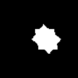
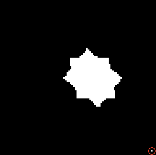
Figure 1: These two binary images only differ by a single pixel, encircled in red on the bottom right of the image on the right. The estimated ellipticity, using (3), is $0.0016+\mathbf{i}0.2196$ for the left image and $-0.0094+\mathbf{i}0.1916$ for the right one. This corresponds to a deviation of 14%.

3 Sparse Deconvolution

Sparsity has proven to be an effective regularization technique for denoising farrens2017space ; starck2015sparse . Its use in deconvolution along with positivity offers satisfying results regarding the pixel error farrens2017space . Sparse regularization is applied in a space where the solution is known to be sparse. In the case of galaxy images, it has been shown in starck2015sparse that starlets offer such a sparse representation.

In the following, we will assume that the noise, $b$ in eq. 1, is white additive Gaussian noise with variance $\sigma^{2}I_{n}$.

Let $\phi=\left(\phi_{i}\right)_{i\in\left\{1,\dots,I\right\}}$ denote the starlet transform operator, with $I$ its chosen number of components. The loss function for the sparse deconvolution problem can be written as the sum of differentiable and non-differentiable terms:

$$L_{0}(x)=\overbrace{\underbrace{\frac{1}{2\sigma^{2}}\|x\ast h-y\|^{2}_{2}}_{\text{data-fidelity}}}^{:=L_{0d}(x),\text{ differentiable}}+\overbrace{\underbrace{\|\lambda_{0}\odot\phi(x)\|_{1}}_{\text{sparsity}}+\underbrace{\iota_{+}(x)}_{\text{positivity}}}^{:=L_{0p}(x),\text{ non-diffrentiable}}\quad,$$ (6)

where $\lambda_{0}$ is a weighting matrix with non-negative entries.

We now give the major properties of $L_{0}$ needed to construct a Sparse Restoration Algorithm (SRA) that minimizes it. Straightforwardly, $L_{0d}$ has gradient

$$\nabla L_{0d}(x)=\frac{1}{2\sigma^{2}}2h_{\pi}\ast\left(x\ast h-y\right)\quad.$$ (7)

Following from its definition, the Lipschitz constant of $\nabla L_{0d}$, noted $\alpha_{0}$, is

$$\alpha_{0}=\frac{1}{2\sigma^{2}}\rho\left(2h_{\pi}\ast h\ast I_{n^{2}}\right)\quad.$$ (8)

Following starck2015sparse , we set the value of $\lambda_{0}$ such that it is proportional to the standard deviation map of $\phi\nabla L_{0d}(x_{T})$. We notice that for $x=x_{T}$, we have $x\ast h-y$ equal to $-b$ which is also a white Gaussian noise of variance $\sigma^{2}I_{n}$. Consequently,

$$\phi_{i}\ast\nabla L_{0d}(x_{T})=-\frac{1}{\sigma^{2}}\phi_{i}\ast h_{\pi}\ast b\quad,\forall i\in\{1,\dots,I\}\,.$$ (9)

It follows that $\phi\nabla L_{0d}(x_{T})$ is colored Gaussian noise, with variance

$$\Sigma_{0}=\underbrace{\frac{1}{\sigma^{2}}\left[\left(\phi_{i}\ast h_{\pi}\ast I_{n^{2}}\right)\left(\phi_{i}\ast h_{\pi}\ast I_{n^{2}}\right)^{\top}\right]_{i\in\{1,\dots,I\}}}_{{:=\left(\Sigma_{0i}\right)}_{i\in\{1,\dots,I\}}}\quad.$$ (10)

We then set

$$\lambda_{0}=\left[\kappa[i]\cdot\text{diag}\left(\Sigma_{0i}\right)\right]_{i\in\{1,\dots,I\}}=\frac{1}{\sigma^{2}}\left(\kappa[i]\cdot\|\phi_{i}\ast h_{\pi}\|^{2}_{2}\mathbf{1}_{n^{2}}\right)_{i\in\{1,\dots,I\}}\quad,$$ (11)

where $\kappa$ is a vector in $\mathbb{R}^{I+1}$ of the form $\left(0,q,\dots,q,q+1\right)$, assuming that the components of $\phi$ are arranged gradually from the coarse scale $\phi_{0}$ to the finest scale $\phi_{I}$. In this work, we set $q=4$.

Finally, we approximate the proximal operator of the non-differentiable part, $L_{0p}$, of the the loss function. To do so, let us first recall the exact forms of the proximal operators of $\iota_{+}$ and $\|\lambda\odot\cdot\|_{1}$, with $\lambda\in\mathbb{R}^{(I+1)\times n\times n}_{+}$:

$$\text{prox}_{\iota_{+}}(x)=(x)_{+}\quad,$$ (12)

where $\forall k\in\{1,\dots,n^{2}\}$,

$$(x)_{+}[k]=\text{max}\left(x[k],0\right)\quad,$$ (13)

and

$$\text{prox}_{\|\lambda\odot.\|_{1}}(x)=\text{ST}_{\lambda}(x)\quad,$$ (14)

where $\text{ST}_{\lambda}$ is the soft-thresholding operator, defined $\forall k\in\{1,\dots,(I+1)n^{2}\}$ as

$$\text{ST}_{\lambda}(x)[k]=\left\{\begin{array}[]{ll}x[k]-\text{sgn}\left(x[k]\right)\lambda\text{ if }\left|x[k]\right|\geq\left|\lambda[k]\right|\\ 0\text{ otherwise}\end{array}\right.\quad.$$ (15)

Nevertheless, in practice, the hard-thresholding operator is preferred over the soft-thresholding in order to reduce the bias introduced by image restoration starck2002nonlinear ; blumensath2009iterative . Let $\text{HT}_{\lambda}$ denote the hard-thresholding operator, defined $\forall k\in\{1,\dots,(I+1)n^{2}\}$ as

$$\text{HT}_{\lambda}(x)[k]=\left\{\begin{array}[]{ll}x[k]\text{ if }\left|x[k]\right|\geq\left|\lambda[k]\right|\\ 0\text{ otherwise}\end{array}\right.\quad.$$ (16)

From these, we define

$$\text{p}_{\lambda_{0}}(x)=\left[\phi^{-1}\left(\text{HT}_{\lambda_{0}}\left[\phi\left(x\right)\right]\right)\right]_{+}\quad,$$ (17)

the approximation of $\text{prox}_{L_{0p}}$ we will use in the present work.
Remark: $\text{p}_{\lambda_{0}}$ relies on two approximations. The first is related to the starlet, which is redundant (thus non-orthogonal), as an orthogonal transform. The second is due to assuming that the proximal operator of the sum of two non-differentiable terms is the composition of the proximal operators of the terms, which does not hold in general.

The implementation of SRA used in this work is based on a proximal splitting frame, more precisely, on forward-backward splitting methods starck2015sparse . The resulting algorithm is given in alg. 1. We still need to set the stopping criterion, $A$; the first-guess, $t\in\mathbb{R}^{n\times n}$; $\alpha_{\epsilon}$ and $\hat{\lambda}_{0}$ which are respectively the estimations of $\alpha_{0}$ and $\lambda_{0}$.

Algorithm 1 SRA algorithm

  Task: Restore $x_{T}$ using $y$ and $h$.

  Parameters: $\gamma$, $\epsilon>0$, boolean $A$.

  Initialization: $x^{(0)}\leftarrow t$, $\beta\leftarrow\alpha_{\epsilon}^{-1}$

  while not$\left(A\right)$ do

     $x^{(i+1)}\leftarrow\text{p}_{\beta\hat{\lambda}}\left[x^{(i)}-\beta\nabla L_{d}\left(x^{(i)}\right)\right]$

     $i\leftarrow i+1$

  end while

  return  $x^{(i)}$

We compute $\alpha_{\epsilon}$ by using the power iteration method to obtain an estimation of $\alpha$, and then we multiply the output by $(1+\epsilon)$ to make sure that we did not go below the lowest upper bound (for this paper, we set $\epsilon=0.05$). $\hat{\lambda}_{0}$ is computed using eq. 11. And we set $t$ to $\frac{1}{n^{2}}\mathbf{1}_{n^{2}}$.

For the stopping criterion, we considered two cases :

The denoising case ($h=\delta$):

here the problem is well-conditioned, and we set $A$ to ‘$i\leq N_{i}$’ where $N_{i}$ is the number of iterations. For the numerical experiments we set $N_{i}$ to 40.

The general case:

here the problem is ill-conditioned, prompting us to set $A$ to ‘$i\leq N_{i}$ and $\left|\frac{\left[L\left(x^{(i)}\right)+L\left(x^{(i-1)}\right)\right]-\left[L\left(x^{(i-2)}\right)+L\left(x^{(i-3)}\right)\right]}{L\left(x^{(i-2)}\right)+L\left(x^{(i-3)}\right)}\right|\leq c$’. In the present experiments, we set $N_{i}=150$ and $c=10^{-6}$.

4 Deconvolution with Shape Constraint

4.1 The Shape Constraint

Ideally, the shape constraint should take the form of a data fidelity term in a space that corresponds to the ellipticity. However the ellipticity, $e(x)$, as defined in eq. 3 is a non-linear function of the galaxy image, $x$. We thus express it as a combination of linear quantities, which will prove easier to handle mathematically. In bernstein2014bayesian , it is shown that the ellipticity can be rewritten using scalar products. Analogously, we derive in appendix A the following formulae:

$$\mathrm{e}_{1}(x)=\frac{\left<x,u_{3}\right>\left<x,u_{5}\right>-\left<x,u_{1}\right>^{2}+\left<x,u_{2}\right>^{2}}{\left<x,u_{3}\right>\left<x,u_{4}\right>-\left<x,u_{1}\right>^{2}-\left<x,u_{2}\right>^{2}}\quad,$$ (18)

$$\mathrm{e}_{2}(x)=\frac{2(\left<x,u_{3}\right>\left<x,u_{6}\right>-\left<x,u_{1}\right>\left<x,u_{2}\right>)}{\left<x,u_{3}\right>\left<x,u_{4}\right>-\left<x,u_{1}\right>^{2}-\left<x,u_{2}\right>^{2}}\quad,$$

with $\left(u_{k}\right)_{k\in\{1,\dots,6\}}$ in $\mathbb{R}^{6\times n\times n}$, defined for all $i$ and $j$ in $\{1,\dots,n\}$ as

$$u_{1}[(i-1)n+j]=(i), u_{2}[(i-1)n+j]=(j),$$ (19)

$$u_{3}[(i-1)n+j]=(1), u_{4}[(i-1)n+j]=(i^{2}+j^{2}),$$

$$u_{5}[(i-1)n+j]=(i^{2}-j^{2}), u_{6}[(i-1)n+j]=(ij).$$

Eq. 18 shows that the ellipticity information is contained in the set of $6$ scalar products. Additionally, in eq. 19, we can see that $\left(u_{k}\right)_{k\in\{1,\dots,6\}}$ are constant vectors. The scalar products are therefore all linear functions of $x$. Consequently, we choose them as building blocks for the shape constraint, instead of directly using the ellipticity (which is not a linear function of $x$). From this, we give a preliminary formulation of the constraint:

$$M_{0}(x)=\sum_{i=1}^{6}\omega_{i}\left<x\ast h-y,u_{i}\right>^{2}\quad,$$ (20)

where the components of $\left(\omega_{i}\right)_{i\in\{1,\dots,6\}}$ are real valued scalar weights.

As discussed in sect. 2, the quantities in eq. 20 are extremely sensitive to noise. A natural way to increase the robustness of our shape constraint would be, in analogy with the ellipticity estimator of eq. 5, to apply a weighting function $g$. This choice, however, comes with the burden of correctly choosing $g$. A fixed window function would lack flexibility and likely lead to poor estimators of ellipticity for some objects $y$. Fitting $g$ to $y$ would improve flexibility, but require an additional preprocessing step.

An alternative approach is to apply the constraint on many windows of different sizes and orientations, so that at least one of them is a good fit to $y$. To find such a set of windows, we consider curvelet-like decompositions starck:sta01_3 ; starck2015sparse where all the bands correspond to windows with different orientations, and every scale corresponds to a different size. Shearlets are particularly appropriate for our ends, as can be seen from Fig. 2. This choice was also motivated by the two following properties kutyniok2012introduction ; voigtlaender2017analysis :

• Anistropy: Ellipticity is, itself, a measure of anisotropy and the use of the shearlets, which are an anisotropic transform, should help us discriminate objects according to this criterion.

• Grid conservation: The scaling and shearing operations that transition from one shearlet band to another conserve the points on the grid, which adds numerical stability.

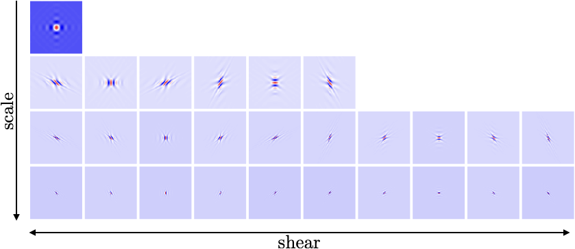
Figure 2: Representation of the shearlet bands with 3 scales.

Let $\psi=\left(\psi_{j}\right)_{j\in\{1,\dots,J\}}$ denote the shearlet transform operator, with $J$ its chosen number of components. We formulate the shape constraint as follows:

$$M(x)=\sum_{i=1}^{6}\sum_{j=1}^{J}\omega_{ij}\left<\psi_{j}(x\ast h)-\psi_{j}(y),u_{i}\right>^{2}\quad,$$ (21)

where $\left(\omega_{ij}\right)_{\begin{subarray}{c}i\in\{1,\dots,6\}\\ j\in\{1,\dots,J\}\end{subarray}}$ are real-valued scalars (see sect. 4.3 for their practical selection). By taking into account the fact that the shearlet transform is a linear operator, and denoting $\psi_{j}^{\ast}$ the adjoint operator of $\psi_{j}$ for all $j$ in $\{1,\dots,J\}$, we have

$$M(x)=\sum_{i=1}^{6}\sum_{j=1}^{J}\omega_{ij}\left<x\ast h-y,\psi_{j}^{\ast}\left(u_{i}\right)\right>^{2}\quad.$$ (22)

Wavelet moments chen2011wavelet ; farokhi2014near and curvelet moments murtagh2008wavelet ; dhahbi2015breast have been similarly used in the past, but only for classification applications.

After formulating the constraint, we will put it into use by adding it to a sparse restoration algorithm that computes a solution to eq. 1. We achieve this by creating the corresponding loss function, exhibiting its properties and, finally, building an algorithm that minimizes it: SCORE.

4.2 The Loss Function

Combining the shape constraint from eq. 22 and the loss function of SRA from eq. 6, we obtain the SCORE loss function,

$$L(x)=\overbrace{\frac{1}{2\sigma^{2}}\|x\ast h-y\|^{2}_{2}+\underbrace{\frac{\gamma}{2\sigma^{2}}M(x)}_{\text{shape constraint}}}^{:=L_{d}(x),\text{ differentiable part}}+\overbrace{\|\lambda\odot\phi(x)\|_{1}+\iota_{+}(x)}^{:=L_{p}(x),\text{ non-diffrentiable part}}\quad,$$ (23)

where $\gamma\in\mathbb{R}_{+}$ is the trade-off between the data-fidelity term and the shape constraint and $\lambda$ is, as before, a weighting matrix with non-negative entries.

Before expressing the main properties of $L$, let us give a reformulation of its differentiable part, $L_{d}$. Namely, let us show that it can be recast as a single data-fidelity term with a modified norm. As a starting point, on the one hand, we have

$$M(x) =\frac{\gamma}{2\sigma^{2}}\sum_{i,j}\omega_{ij}\left<x\ast h-y,\psi_{j}^{\ast}\left(u_{i}\right)\right>^{2}\quad,$$ (24)

$$=\frac{\gamma}{2\sigma^{2}}\sum_{i,j}\omega_{ij}\left(\left[\psi_{j}^{\ast}\left(u_{i}\right)\right]^{\top}\left[x\ast h-y\right]\right)^{\top}\left(\left[\psi_{j}^{\ast}\left(u_{i}\right)\right]^{\top}\left[x\ast h-y\right]\right),$$ (25)

$$=\frac{1}{2\sigma^{2}}\left(x\ast h-y\right)^{\top}\gamma\underbrace{\sum_{i,j}\overbrace{\omega_{ij}\psi_{j}^{\ast}\left(u_{i}\right)\left[\psi_{j}^{\ast}\left(u_{i}\right)\right]^{\top}}^{:=Q_{ij}\succeq 0}}_{:=Q\succeq 0}\left(x\ast h-y\right)\quad.$$ (26)

Similarly, on the other hand, we have

$$\frac{1}{2\sigma^{2}}\|x\ast h-y\|^{2}_{2}=\frac{1}{2\sigma^{2}}\left(x\ast h-y\right)^{\top}I_{n}\left(x\ast h-y\right)\quad.$$ (27)

By summing eq. 26 and 27, we obtain

$$L_{d}(x) =\frac{1}{2\sigma^{2}}\left(x\ast h-y\right)^{\top}\underbrace{\left(I_{n}+\gamma Q\right)}_{:=S\succ 0}\left(x\ast h-y\right)\quad,$$ (28)

$$L_{d}(x) =\frac{1}{2\sigma^{2}}\|x\ast h-y\|_{S}\quad.$$ (29)

We can thus interpret the weighted data-fidelity term in eq. 29 as an extension of the space of the data-fidelity. When using it, we are effectively not only considering the image space by itself, but also taking the space of scalar products of $M$ into account.

4.3 Properties of $L$

Analogously to sect. 3, we first determine the values of the constants (other than $\gamma$, which we study in detail in sect. 5.1) that appear in $L$, and how to handle its differentiable and non-differentiable parts within an optimization framework.

To determine $\left(\omega_{ij}\right)_{\begin{subarray}{c}i\in\{1,\dots,6\}\\ j\in\{1,\dots,J\}\end{subarray}}$ in (22), let us impose that the unweighted data-fidelity and the shape constraint exert the same relative influence when $\gamma$ is 1. In addition, without any further prior, we want all components of $Q$ to have equal influence. With no guarantee of orthogonality, we then impose the following conditions

$$\left\{\begin{array}[]{ll}\|I_{n}\|_{\text{F}}=\displaystyle\sum_{i=1}^{6}\sum_{j=1}^{J}\|Q_{ij}\|_{\text{F}}\quad,\\ \|Q_{ij}\|_{\text{F}}=\|Q_{kl}\|_{\text{F}}\quad,\,\forall i,k\in\left\{1,\dots,6\right\}\quad,\,\forall j,l\in\left\{1,\dots,J\right\}.\end{array}\right.$$ (30)

Solving the system in 30, leads to:

$$\omega_{ij}=\frac{n}{\left\|\psi_{j}^{*}\left(u_{i}\right)\right\|_{2}^{2}}\quad,\,\forall i\in\{1,\dots,6\}\,,\,\forall j\in\{1,\dots,J\}.$$ (31)

The gradient of $L_{d}$ follows from eq. 28:

$$\nabla L_{d}(x)=\frac{1}{2\sigma^{2}}2h_{\pi}\ast S\left(x\ast h-y\right)\quad.$$ (32)

Its Lipschitz constant, noted $\alpha$, is

$$\alpha=\frac{1}{2\sigma^{2}}\rho\left(2h_{\pi}\ast h\ast S\right)\quad.$$ (33)

In order to set $\lambda$, we once again propagate residual noise. Since

$$\phi_{i}\ast\nabla L_{d}(x)=-\frac{1}{\sigma^{2}}\phi_{i}\ast h_{\pi}\ast Sb\quad,\forall i\in\{1,\dots,I\}\,,$$ (34)

$\phi L_{d}(x)$ is colored Gaussian noise, with variance

$$\Sigma=\underbrace{\frac{1}{\sigma^{2}}\left[\left(\phi_{i}\ast h_{\pi}\ast S\right)\left(\phi_{i}\ast h_{\pi}\ast S\right)^{\top}\right]_{i\in\{1,\dots,I\}}}_{:=\left(\Sigma_{i}\right)_{i\in\{1,\dots,I\}}}\quad.$$ (35)

This allows us to chose

$$\lambda=\left[\kappa[i]\cdot\text{diag}\left(\Sigma_{i}\right)\right]_{i\in\{1,\dots,I\}}\quad.$$ (36)

Lastly, similar to sect. 4.2, we approximate $\text{prox}_{L_{p}}$ by

$$\text{p}_{\lambda}(x)=\left[\phi^{-1}\left(\text{HT}_{\lambda}\left[\phi\left(x\right)\right]\right)\right]_{+}\quad.$$ (37)

4.4 Algorithm

The SCORE algorithm is given in alg. 2. As with sect. 3, we also need to set the stopping criterion, $A$; the first-guess, $t\in\mathbb{R}^{n\times n}$; $\alpha_{\epsilon}$ and $\hat{\lambda}$ which are respectively the estimations of $\alpha$ and $\lambda$.

Algorithm 2 SCORE algorithm

  Task: Restore $x_{T}$ using $y$ and $h$.

  Parameters: $\gamma$, $\epsilon>0$, boolean $A$.

  Initialization: $x^{(0)}\leftarrow t$, $\beta\leftarrow\alpha_{\epsilon}^{-1}$

  while not$\left(A\right)$ do

     $x^{(i+1)}\leftarrow\text{p}_{\beta\hat{\lambda}}\left[x^{(i)}-\beta\nabla L_{d}\left(x^{(i)}\right)\right]$

     $i\leftarrow i+1$

  end while

  return  $x^{(i)}$

As for alg. 1, we compute $\alpha_{\epsilon}$ by using the power iteration method to obtain an estimation of $\alpha$, and then multiplying the output by $(1+\epsilon)$ (for this paper, $\epsilon=0.05$). For the other variables, we considered:

The denoising case ($h=\delta$):

here the problem is well-conditioned, therefore we set $A$ to ‘$i\leq N_{i}$’ where $N_{i}$ is the number of iterations. To set $t$, we gave it the value of the output of SRA. Finally, we directly compute $\hat{\lambda}$ using the formula in eq. 36.

The general case:

here the problem is ill-conditioned, which leads us to set $A$ to ‘$i\leq N_{i}$ and $\left|\frac{\left[L\left(x^{(i)}\right)+L\left(x^{(i-1)}\right)\right]-\left[L\left(x^{(i-2)}\right)+L\left(x^{(i-3)}\right)\right]}{L\left(x^{(i-2)}\right)+L\left(x^{(i-3)}\right)}\right|\leq c$’. We choose the first guess $t=\frac{1}{n^{2}}\mathbb{1}$. To compute $\hat{\lambda}$, we generate $G$ realisations of white Gaussian noise of variance $\sigma^{2}I_{n^{2}}$. In this paper, we set $c$ to $10^{-6}$ and $G$ to 100.

Assuming that each image contains only one galaxy such that all of its active pixels are connected, we add a post-processing step to remove the other isolated blobs in the output image. To do so, we mask the isolated blobs by first binarizing each output image using its 80^th percentile pixel value as a threshold. Then, under the safe assumption that the galaxy of interest should correspond to the largest blob, we set every other blob’s pixels to 0.

5 Numerical Experiments

In this section, we perform numerical experiments on simulated galaxy images. We start by describing the dataset, then detail the implementation framework used. We also present two experiments, one on denoising and one on deconvolution.

5.1 Dataset & Implementation

To build our dataset, we generate 300 galaxy images, simulated using parameters fitted on real galaxies from the catalog COSMOS Mandelbaum_2011 and 300 PSF images with a Moffat profile. Each image has $96\times 96$ pixels. For further details on the data generation, see appendix  B. To create the observations, we convolve each galaxy with a PSF then add noise.

Regarding noise levels, we use the following definition for the signal-to-noise ratio (SNR) of an observation $y$ of $x_{T}$:

$$\text{SNR}(y)=\frac{\left\|x_{T}\right\|_{2}}{\sigma}\quad.$$

The chosen SNR levels are 40, 75, 150 and 380, with 300 observations generated for each.

The implementation was done using Python 3.6.8, ModOpt 1.3.0, Alpha-Transform and Matplotlib hunter2007matplotlib .

In order to study the influence of $\gamma$ from eq. 23, we perform a two-step grid search by first determining the magnitude of the optimal parameter, then testing a finer grid of values in that range. The criterion chosen is

$$\gamma_{*}=\underset{\gamma}{\text{argmin }}\delta_{e}(\gamma)\quad,\text{where }\delta_{e}(\gamma)=\underset{i}{\text{mean}}\left[\text{MSE}\left(e\left(\hat{x}_{\gamma,i}\right)\right)\right],$$ (38)

such that $\underset{i}{\text{mean}}(x_{i})$ is the mean of $\left(x_{i}\right)_{i}$ over $i$ and $\hat{x}_{\gamma,i}$ is the SCORE estimation of the $i^{th}$ galaxy with trade-off parameter equal to $\gamma$. The resulting $\gamma_{*}$ are shown, per SNR level, in Table 1. Its value is close to 1 in all cases.

Table 1: Values of $\gamma_{\ast}$.

SNR	Denoising	Full restoration
40	1.2	1.2
75	0.8	1.6
150	1.0	1.2
380	0.8	0.6

5.2 Results

Denoising

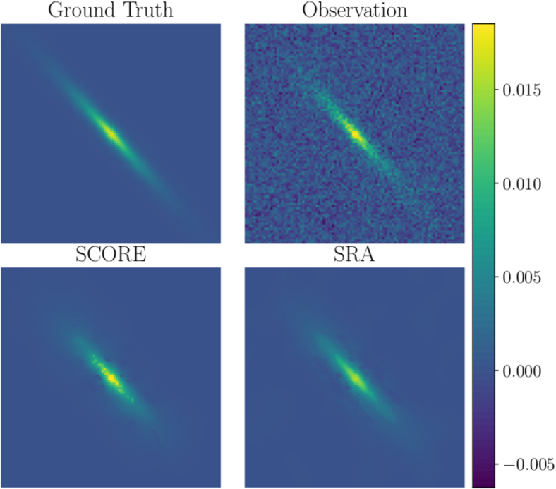
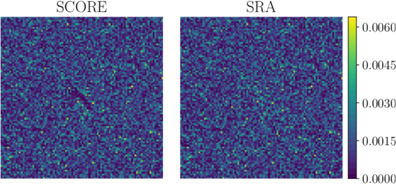
Figure 3: Denoising results of galaxy #38 for SNR=75. Top: original image and observed data (i.e. blurred image with noise). Center: denoised images with SCORE and SRA. Bottom: residual images with SCORE and SRA.

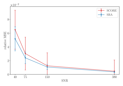
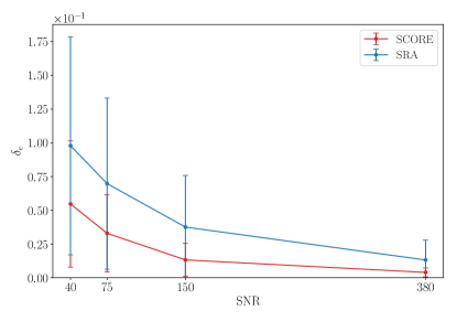
Figure 4: Left: relative MSE per SNR of the galaxies for the denoising experiment. Right: ellipticity error $\delta_{e}$ per SNR. In both cases, the curves correspond to the mean per SNR and the vertical bars to the standard deviation.

We first consider the denoising case ($h=\delta$). The top row of Fig. 3 shows an example of an original galaxy image and its corresponding degraded observation, the center row shows the denoised images with both SCORE and SRA, and the bottom row the corresponding residual images. Fig. 4 shows the MSE and ellipticity errors $\delta_{e}$ as a function of SNR.

We can see that SCORE leads to a slight degradation in pixel MSE, compared to SRA. This is not unexpected as the latter’s data fidelity term is entirely expressed in the image domain, while that of SCORE is shared with a shape component, as shown in sect. 4.2. SCORE’s ellipticity errors are significantly reduced, by a factor of about 2.

Deconvolution

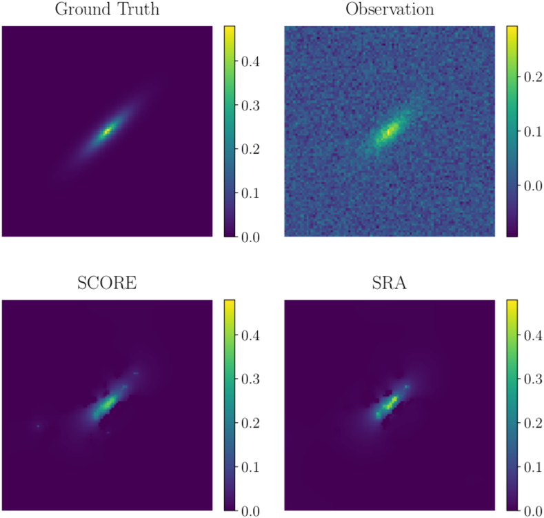
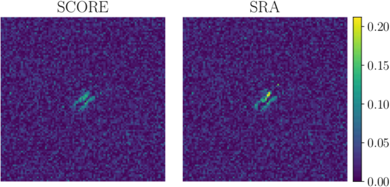
Figure 5: Deconvolution results of galaxy #16 for SNR=75. Top: original image and observed data (i.e. blurred image with noise). Center: deconvolved images with SCORE and SRA. Bottom: residual images for SCORE and SRA, using the same color bar.

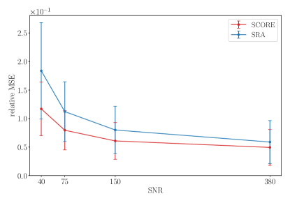
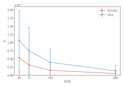
Figure 6: Same as Fig. 4, for the deconvolution experiment.

Similarly, Fig. 5 shows an example galaxy, its recovered profiles with both approaches, and the corresponding residuals, while Fig. 6 shows the distributions of pixel and ellipticity errors at all SNRs.

In the case of deconvolution, SCORE performs better than SRA for both MSE and ellipticity errors. Indeed, the MSE yielded by SCORE is lower by at least 16% (and 36.3% at most) compared to SRA. The example of Fig. 6 illustrates that SCORE’s output has a smoother profile, with a better restoration of the tail of the galaxy compared to SRA. Additionally, the residual of SCORE is, towards the center of the object, fainter than that of SRA.

We observe different trends when looking at pixel MSE between the denoising case and the full restoration one. We believe this is due to the different conditioning of the two problems. The deconvolution is more ill-conditioned than a simple denoising. Therefore, the broader the space of solutions, the higher the chance that an additional constraint would bring the solution closer to the ground truth.

In terms of ellipticity, SCORE’s $\delta_{e}$ is not only lower than SRA, but seems also less biased and more consistent according to the error bars. In the denoising case, it is 44.1% at least (and 70.3% at most) lower, and in the deconvolution case, 49.5% at least (and 62.3% at most). Figs. 3 and 5 show that the galaxy’s profile and its shape are better preserved with SCORE than with SRA.

6 Reproducible Research

In the spirit of repeatable and reproducible research, all the codes and the resulting material have been made publicly available on GitHub at the following link: https://github.com/CosmoStat/score. In addition, at the end of the description of each figure, this icon provides a hyperlink to a Jupyter Notebook that shows how to generate the figure.

7 Conclusion

In order to better preserve the shapes of galaxies during a restoration process, we have proposed a new regularization term, based on the second-order moments. We have shown that our shape constraint can easily be plugged into a sparse recovery algorithm, leading to a new method called SCORE. For denoising, when comparing to sparse recovery, we have shown that adding the shape constraint leads to a trade-off between the mean square error and the galaxy ellipticity error, where the latter is reduced by at least 44.1%, while the MSE is, however, increased by at most 28.5%. For deconvolution, both are improved (by at least 49.5% for the ellipticity error and 16.9% for the MSE). We believe this different behavior between denoising and deconvolution is due to the fact that the space of potential solutions is large in the deconvolution case, and that the additive shape regularizing term helps to better constrain the inverse problem.

Additionally, SCORE contains only one parameter that cannot be chosen analytically, namely the trade-off between the data-fidelity and the shape constraint terms, $\gamma$.

We have used in this paper the Forward-Backward sparse deconvolution algorithm for its simplicity, but any more recent proximal algorithm such as Condat-Vu Condat11 ; Vu11 could be used as well. The shape constraint could also easily be added to other existing deconvolution techniques, such as Total Variation weiss-tv-nesterov or deep learning deepmassJ ; sureau2019deep . Finally, the shape constraint could also be improved by using moments at higher orders and also in different spaces  flusser20162d ; kostkova2019image ; shakibaei2014image ; wojak2010introducing .

Appendix A Expressing Galaxy Ellipticity with Inner Products

Assume that we have $x\in\mathbb{R}^{n\times n}$ such that

$$\mathrm{e}(x)=\frac{\mu_{2,0}(x)-\mu_{0,2}(x)+2i\mu_{1,1}}{\mu_{2,0}(x)+\mu_{0,2}(x)}\quad,$$ (39)

where $\mu_{s,t}$ is a centered moment of order $(s+t)$, defined as follows :

$$\mu_{s,t}(x)=\sum_{i=1}^{n}\sum_{j=1}^{n}x\left[(i-1)n+j\right](i-i_{c})^{s}(j-j_{c})^{t}\quad,$$ (40)

and $(i_{c},j_{c})$ are the coordinates of the centroid of the two dimensional image encoded by $x$ :

$$i_{c}=\frac{\sum_{i=1}^{n}\sum_{j=1}^{n}i\cdot x[(i-1)n+j]}{\sum_{i=1}^{n}\sum_{j=1}^{n}x[(i-1)n+j]}\text{ and }j_{c}=\frac{\sum_{i=1}^{n}\sum_{j=1}^{n}j\cdot x[(i-1)n+j]}{\sum_{i=1}^{n}\sum_{j=1}^{n}x[(i-1)n+j]}\quad.$$ (41)

We want to show that

$$\mathrm{e}(x)=\frac{\left<x,u_{3}\right>\left<x,u_{5}\right>-\left<x,u_{1}\right>^{2}+\left<x,u_{2}\right>^{2}+2i\left(\left<x,u_{3}\right>\left<x,u_{6}\right>-\left<x,u_{1}\right>\left<x,u_{2}\right>\right)}{\left<x,u_{3}\right>\left<x,u_{4}\right>-\left<x,u_{1}\right>^{2}-\left<x,u_{2}\right>^{2}}\quad,$$ (42)

where $\forall i,j\in\{1,\dots,n\}$,

$$u_{1}[(i-1)n+j]=(i), u_{2}[(i-1)n+j]=(j),$$ (43)

$$u_{3}[(i-1)n+j]=(1), u_{4}[(i-1)n+j]=(i^{2}+j^{2}),$$

$$u_{5}[(i-1)n+j]=(i^{2}-j^{2}), u_{6}[(i-1)n+j]=(ij).$$

To do so, we only have to express $\mu_{0,2}(x)$; $\mu_{1,1}(x)$ and $\mu_{2,0}(x)$ using $\left(\left<x,u_{i}\right>\right)_{1\leq i\leq 6}$. We start by introducing $m_{s,t}(x)$, the non-centered moment of order $(s+t)$,

$$m_{s,t}=\sum_{i=1}^{n}\sum_{j=1}^{n}x\left[(i-1)n+j\right]i^{s}j^{t}\quad.$$ (44)

We then express $\mu_{0,2}(x)$; $\mu_{1,1}(x)$ and $\mu_{2,0}(x)$ using the non-centered moments (of order equal or less than 2), as follows:

$$\mu_{0,2}(x) =m_{0,2}(x)-\frac{m^{2}_{0,1}(x)}{m_{0,0}(x)}\quad,$$ (45)

$$\mu_{1,1}(x) =m_{1,1}(x)-\frac{m_{0,1}(x)\cdot m_{1,0}(x)}{m_{0,0}(x)}\quad,$$

$$\mu_{2,0}(x) =m_{2,0}(x)-\frac{m^{2}_{1,0}(x)}{m_{0,0}(x)}\quad.$$

Expressing these non-centered moments using $\left(\left<x,u_{i}\right>\right)_{1\leq i\leq 6}$, we obtain

$$m_{0,0}(x)=\left<x,u_{3}\right>, m_{1,0}(x)=\left<x,u_{1}\right>,$$ (46)

$$m_{0,1}(x)=\left<x,u_{2}\right>, m_{1,1}(x)=\left<x,u_{6}\right>,$$

$$m_{0,2}(x)=\frac{1}{2}\left(\left<x,u_{4}\right>-\left<x,u_{5}\right>\right), m_{2,0}(x)=\frac{1}{2}\left(\left<x,u_{4}\right>+\left<x,u_{5}\right>\right).$$

Using eq. 45 and  46, we can express $\mu_{0,2}(x)$, $\mu_{1,1}(x)$, and $\mu_{2,0}(x)$ using $\left(\left<x,u_{i}\right>\right)_{1\leq i\leq 6}$:

$$\mu_{0,2}(x) =\frac{1}{2}\left(\left<x,u_{4}\right>-\left<x,u_{5}\right>\right)-\frac{\left<x,u_{2}\right>^{2}}{\left<x,u_{3}\right>},$$ (47)

$$\mu_{1,1}(x) =\left<x,u_{6}\right>-\frac{\left<x,u_{1}\right>\left<x,u_{2}\right>}{\left<x,u_{3}\right>},$$

$$\mu_{2,0}(x) =\frac{1}{2}\left(\left<x,u_{4}\right>+\left<x,u_{5}\right>\right)-\frac{\left<x,u_{1}\right>^{2}}{\left<x,u_{3}\right>}.$$

We finish the proof by inserting eq. 47 in eq. 39 to obtain eq. 42.

Appendix B Dataset Generation

To generate the galaxy and the PSF images, we chose simple and commonly used profiles in astrophysics which are repectively Sersic and Moffat profiles. First, the light intensity $I_{G}$ of a galaxy is modeled with a Sersic using the following formula:

$$I_{G}(R)=I_{e}\cdot\text{exp}\left(b_{n}\left[\left(\frac{R}{R_{e}}\right)^{\frac{1}{n}}-1\right]\right)\quad,$$ (48)

where $n\in\mathbb{R}_{+}$ is the Sersic index, $R_{e}$ is the half-light radius, $I_{e}$ is the light intensity at $R_{e}$ and $b_{n}$ satisfies $\gamma(2n;b_{n})=\frac{1}{2}\Gamma(2n)$ with $\Gamma$ and $\gamma$ respectively the Gamma function and the lower incomplete gamma function. We draw the values of the parameters $n$, $I_{e}$ and $R_{e}$ from the catalog COSMOS Mandelbaum_2011 to generate isotropic galaxy images to which we will later give a non-zero ellipticity.

Second, the light intensity $I_{P}$ of a PSF is modeled with a Moffat profile using the following formula:

$$I_{P}(R)=2\frac{\beta-1}{\sigma^{2}}\left(1+\left[\frac{R}{\sigma}\right]^{2}\right)^{-\beta}\quad,$$ (49)

where $\beta$ is set to 4.765 (cf. ref. trujillo2001effects ) and $\sigma$ is calculated using the following relation:

$$\text{FWHM}=2\sigma\sqrt{2^{\frac{1}{\beta}}-1}\quad,$$ (50)

where FWHM is the Full Width Half Maximum of the Moffat profile. Its value is drawn from a uniform distribution between 0.1 and 0.2 arcsec, which correspond respectively to Hubble Space Telescope and Euclid space telescope observations. This gives us preliminary, isotropic PSF images.

We finally give an ellipticity to the both these galaxy and PSF images. To do so, we draw the values of the ellipticity components from a centered normal distribution truncated between -1 and 1. The standard deviations are chosen as 0.3 for the galaxies and 0.03 for the PSF bernstein2014bayesian .

References

- (1) Bartelmann, M., Schneider, P.: Weak gravitational lensing. Physics Reports 340(4-5), 291–472 (2001)
- (2) Bernstein, G.M., Armstrong, R.: Bayesian lensing shear measurement. Monthly Notices of the Royal Astronomical Society 438(2), 1880–1893 (2014)
- (3) Bertero, M., Boccacci, P.: Introduction to inverse problems in imaging. CRC press (1998)
- (4) Blumensath, T., Davies, M.E.: Iterative hard thresholding for compressed sensing. Applied and computational harmonic analysis 27(3), 265–274 (2009)
- (5) Chambolle, A., Caselles, V., Cremers, D., Novaga, M., Pock, T.: An introduction to total variation for image analysis. Theoretical foundations and numerical methods for sparse recovery 9(263-340), 227 (2010)
- (6) Chen, G., Xie, W.: Wavelet-based moment invariants for pattern recognition. Optical Engineering 50(7), 077205 (2011)
- (7) Condat, L.: A generic first-order primal-dual method for convex optimization involving Lipschitzian, proximable and linear composite terms. J. Optimization Theory and Applications 158(2), 460–479 (2013)
- (8) Dhahbi, S., Barhoumi, W., Zagrouba, E.: Breast cancer diagnosis in digitized mammograms using curvelet moments. Computers in biology and medicine 64, 79–90 (2015)
- (9) Farokhi, S., Shamsuddin, S.M., Sheikh, U.U., Flusser, J., Khansari, M., Jafari-Khouzani, K.: Near infrared face recognition by combining zernike moments and undecimated discrete wavelet transform. Digital Signal Processing 31, 13–27 (2014)
- (10) Farrens, S., Mboula, F.N., Starck, J.L.: Space variant deconvolution of galaxy survey images. Astronomy & Astrophysics 601, A66 (2017)
- (11) Flusser, J., Suk, T., Zitova, B.: 2D and 3D Image Analysis by Moments. John Wiley & Sons (2016)
- (12) Hirata, C., Seljak, U.: Shear calibration biases in weak-lensing surveys. Monthly Notices of the Royal Astronomical Society 343(2), 459–480 (2003)
- (13) Hunter, J.D.: Matplotlib: A 2d graphics environment. Computing in science & engineering 9(3), 90 (2007)
- (14) Jeffrey, N., Lanusse, F., Lahav, O., Starck, J.L.: Deep learning dark matter map reconstructions from DES SV weak lensing data. MNRAS492(4), 5023–5029 (2020). DOI 10.1093/mnras/staa127
- (15) Kaiser, N., Squires, G., Broadhurst, T.: A method for weak lensing observations. arXiv preprint astro-ph/9411005 (1994)
- (16) Kostková, J., Flusser, J., Lébl, M., Pedone, M.: Image invariants to anisotropic gaussian blur. In: Scandinavian Conference on Image Analysis, pp. 140–151. Springer (2019)
- (17) Kumar, A.: Deblurring of motion blurred images using histogram of oriented gradients and geometric moments. Signal Processing: Image Communication 55, 55–65 (2017)
- (18) Kutyniok, G., Labate, D.: Introduction to shearlets. In: Shearlets, pp. 1–38. Springer (2012)
- (19) Mandelbaum, R.: Weak lensing for precision cosmology. Annual Review of Astronomy and Astrophysics 56, 393–433 (2018)
- (20) Mandelbaum, R., Hirata, C.M., Leauthaud, A., Massey, R.J., Rhodes, J.: Precision simulation of ground-based lensing data using observations from space. Monthly Notices of the Royal Astronomical Society 420(2), 1518–1540 (2011). DOI 10.1111/j.1365-2966.2011.20138.x. URL http://dx.doi.org/10.1111/j.1365-2966.2011.20138.x
- (21) Miller, L., Kitching, T., Heymans, C., Heavens, A., Van Waerbeke, L.: Bayesian galaxy shape measurement for weak lensing surveys–i. methodology and a fast-fitting algorithm. Monthly Notices of the Royal Astronomical Society 382(1), 315–324 (2007)
- (22) Murtagh, F., Starck, J.L.: Wavelet and curvelet moments for image classification: application to aggregate mixture grading. Pattern Recognition Letters 29(10), 1557–1564 (2008)
- (23) Patel, P.: Weak Lensing with Radio Continuum Surveys. arXiv e-prints arXiv:1602.07482 (2016)
- (24) Patel, P., Abdalla, F.B., Bacon, D.J., Rowe, B., Smirnov, O.M., Beswick, R.J.: Weak lensing measurements in simulations of radio images. MNRAS444(3), 2893–2909 (2014). DOI 10.1093/mnras/stu1588
- (25) Rivi, M., Lochner, M., Balan, S., Harrison, I., Abdalla, F.: Radio galaxy shape measurement with hamiltonian monte carlo in the visibility domain. Monthly Notices of the Royal Astronomical Society 482(1), 1096–1109 (2019)
- (26) Rivi, M., Miller, L., Makhathini, S., Abdalla, F.B.: Radio weak lensing shear measurement in the visibility domain - I. Methodology. MNRAS463, 1881–1890 (2016). DOI 10.1093/mnras/stw2041
- (27) Rodríguez, S., Padilla, N.D., García Lambas, D.: The effects of environment on the intrinsic shape of galaxies. MNRAS456(1), 571–577 (2016). DOI 10.1093/mnras/stv2660
- (28) Rudin, L.I., Osher, S., Fatemi, E.: Nonlinear total variation based noise removal algorithms. Physica D: nonlinear phenomena 60(1-4), 259–268 (1992)
- (29) Shakibaei, B.H., Flusser, J.: Image deconvolution in the moment domain. Moments and Moment Invariants—Theory and Applications 1, 111–125 (2014)
- (30) Starck, J.L.: Nonlinear multiscale transforms. In: Multiscale and multiresolution methods, pp. 239–278. Springer (2002)
- (31) Starck, J.L., Candès, E., Donoho, D.: The curvelet transform for image denoising. IEEE Transactions on Image Processing 11(6) (2002). 131–141
- (32) Starck, J.L., Murtagh, F., Fadili, J.: Sparse image and signal processing: Wavelets and related geometric multiscale analysis. Cambridge university press (2015)
- (33) Sureau, F., Lechat, A., Starck, J.L.: Deep learning for a space-variant deconvolution in galaxy surveys. Astronomy & Astrophysics 641, A67 (2020)
- (34) Trujillo, I., Aguerri, J., Cepa, J., Gutiérrez, C.: The effects of seeing on sérsic profiles–ii. the moffat psf. Monthly Notices of the Royal Astronomical Society 328(3), 977–985 (2001)
- (35) Viola, M., Melchior, P., Bartelmann, M.: Biases in, and corrections to, ksb shear measurements. Monthly Notices of the Royal Astronomical Society 410(4), 2156–2166 (2011)
- (36) Voigtlaender, F., Pein, A.: Analysis vs. synthesis sparsity for -shearlets. arXiv preprint arXiv:1702.03559 (2017)
- (37) Vũ, B.: A splitting algorithm for dual monotone inclusions involving cocoercive operators. Advances in Computational Mathematics 38(3), 667–681 (2013)
- (38) Weiss, P., Blanc-Féraud, L., Aubert, G.: Efficient schemes for total variation minimization under constraints in image processing. SIAM Journal on Scientific Computing 31(3) (2009). 2047–2080
- (39) Wojak, J., Angelini, E.D., Bloch, I.: Introducing shape constraint via legendre moments in a variational framework for cardiac segmentation on non-contrast ct images. In: VISAPP, pp. 209–214 (2010)