UAV-Assisted Over-the-Air Computation

Abstract

Over-the-air computation (AirComp) provides a promising way to support ultrafast aggregation of distributed data. However, its performance cannot be guaranteed in long-distance transmission due to the distortion induced by the channel fading and noise. To unleash the full potential of AirComp, this paper proposes to use a low-cost unmanned aerial vehicle (UAV) acting as a mobile base station to assist AirComp systems. Specifically, due to its controllable high-mobility and high-altitude, the UAV can move sufficiently close to the sensors to enable line-of-sight transmission and adaptively adjust all the links’ distances, thereby enhancing the signal magnitude alignment and noise suppression. Our goal is to minimize the time-averaging mean-square error for AirComp by jointly optimizing the UAV trajectory, the scaling factor at the UAV, and the transmit power at the sensors, under constraints on the UAV’s predetermined locations and flying speed, sensors’ average and peak power limits. However, due to the highly coupled optimization variables and time-dependent constraints, the resulting problem is non-convex and challenging. We thus propose an efficient iterative algorithm by applying the block coordinate descent and successive convex optimization techniques. Simulation results verify the convergence of the proposed algorithm and demonstrate the performance gains and robustness of the proposed design compared with benchmarks.

I Introduction

In the future Internet-of-Things (IoT) based big data applications, both the ultrafast data collection from massive sensors with limited spectrum bandwidth and effective interpretation on collected data with limited computation capacity are highly challenging. For example, in the scenario of environmental monitoring, multiple sensors distributed over a particular area concurrently transmit their measured environmental data (e.g., temperature and humidity), while the monitor needs to receive and compute the average value of the measured data. To tackle these issues, over-the-air computation (AirComp) has recently been proposed as a promising multiple access scheme, which integrates the computation into communication [1], [2]. The basic principle of AirComp is to exploit the waveform superposition property of multiple-access channel (MAC) to compute a class of nomographic functions (e.g., mean and weighted sum) of numerous data via concurrent transmission. Furthermore, this can enable a series of IoT applications ranging from latency-sensitive sensing [3, 4, 5] to data-intensive federated machine learning [2],[6].

In practice, the performance of AirComp is significantly limited by the signal distortion due to channel fading and noise, especially in long-distance transmission. Note that the noise power is comparable to the signal power in long-distance transmission due to analog transmission in most AirComp systems. To enable reliable AirComp, the key designs in AirComp are the power control at sensors for coping with channel attenuation and signal scaling at the base station (BS) for noise suppression [4, 7]. In prior works, uniform channel inversion is implemented at the sensor to perfectly align the magnitude of signals [2, 3, 4]. However, this scheme may severely degrade the AirComp performance when one or more individual channels are in deep fading, which will amplify the negative effect of noise. Recently, the authors in [7] proposed an optimal policy with threshold-based structure to combine channel inversion and full power transmission. As shown in [7], enlarging noise suppression can lead to an increased signal misalignment error since the sensors are usually power constrained. Therefore, due to the channel fading and noise as well as limited transmit power at sensors, relying only on the terrestrial BSs may not be able to guarantee the performance of AirComp in long-distance transmission, especially when the BSs are sparsely deployed or unavailable (e.g., wild-area monitoring applications).

As a remedy to the above limitations, low-cost unmanned aerial vehicle (UAV) is considered as a promising alternative to assist the terrestrial networks [8, 9, 10]. Recently, the research efforts have been devoted to employing UAVs as mobile BSs in IoT networks, such as information dissemination [11, 12], one-by-one data collection [13]. In this paper, we shall propose to deploy the UAV-mounted BS to assist AirComp, thereby enjoying the following advantages compared with the conventional BS. First, the UAV-mounted BS is cost-effective and can move sufficiently close to the sensors even in the wild area, which can avoid long-distance transmission and thus save the sensors’ power and mitigate the effect of noise. Second, due to its high altitude, UAV usually have line-of-sight (LoS) connection with ground sensors, which can reduce the probability of channels in deep fading and thus enhance signal magnitude alignment. Furthermore, the controllable high-mobility UAV can actively construct favorable channels to strike a balance between communication distance and sensors’ heterogeneous power constraints. Specifically, UAV can dynamically adapt its trajectory to fly closer to sensors with lower power than these with higher power to align the magnitude of signals, which possess an additional degree of freedom for the AirComp performance enhancement. Hence, this motivates us to study a new AirComp technique referred to as UAV-assisted AirComp, which has the potential to overcome the issues of conventional AirComp.

In this paper, we consider a UAV-assisted AirComp system, in which the UAV acting as a mobile BS is dispatched to collect average information of distributed data generated by ground sensors via AirComp during a given mission interval. A common design metric that has been widely adopted in AirComp is the mean-squared error (MSE) between the estimated function value and the target function value [2, 3, 7, 4]. Hence, our goal is to minimize the time-average MSE by jointly optimizing the UAV trajectory, signal scaling factor (termed as denoising factor) at UAV, and transmit power at ground sensors. However, due to the highly coupled variables and time-dependent constraints, it is challenging to solve the resulting problem optimally in general. To address these challenges, we develop an efficient iterative algorithm by applying the block coordinate descent method, where the transmit power, denoising factor, and UAV trajectory are optimized in an alternating manner. However, the UAV trajectory optimization subproblem is still difficult to be solved due to the non-convexity of its objective function, for which the successive convex approximation is applied to solve it approximately. The numerical results validate the convergence of the proposed algorithm. It is also observed that UAV trajectory design can dynamically adapt to different transmit power, the proposed joint design can achieve significant performance gains and the robustness, as compared to the benchmarks.

II System Model and Problem Formulation

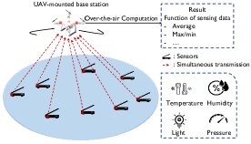
Figure 1: UAV-assisted AirComp networks

As illustrated in Fig. 1, we consider a UAV-assisted AirComp network with $K$ ground sensors. Both the UAV and sensors are equipped with a single antenna due to their size and power limitations. The mobile UAV is interesting in exploiting the AirComp to aggregate the average function of distributed data generated by $K$ ground sensors during a given flight time $T$ second (s) rather than obtaining the value of each individual data. Therein, due to its controllable high-mobility and high-altitude, UAV can move sufficiently close to sensors with LoS connections and adaptively balance between communication distance and sensors’ transmit power, which can save sensors’ power for the signal magnitude alignment and suppress noise. One practical scenario for such a consideration could be wild-area environmental monitoring when the BSs are unavailable nearby, where the UAV is employed to monitor the average value of the temperature measured by sensors distributed over a particular area. Note that we focus on the basic scenario with a single UAV and without conventional terrestrial BS. The extension to consider more general cases with multiple cooperative UAVs and/or in the presence of ground BSs will be left as our future work.

We consider a three-dimensions (3D) Cartesian coordinate system, where the horizontal coordinate of sensor $k$ is denoted as $\mathbf{w}_{k}=[x_{k},y_{k}]\in\mathbb{R}^{1\times 2}$ with $x_{k}$ and $y_{k}$ being $x$- and $y$- coordinates, respectively. The set of ground sensors is denoted as $\mathcal{K}\triangleq\{1,\ldots,K\}$, $K>1$. During the flight of the UAV, the ground sensors’ locations are assumed to be fixed and known to the UAV. In practice, the locations of sensors could be determined by the standard positioning techniques (e.g., GPS based localization). Additionally, we assume that the UAV flies at a fixed altitude $H$ above the ground level. Note that in practice, $H$ corresponds to the minimum altitude that ensures obstacle avoidance without the need for frequent aircraft ascending and descending.

II-A UAV Trajectory Model and Channel Model

We denote the time-varying UAV trajectory projected on the horizontal plane as $\bm{q}(t)=[x(t),y(t)]\in\mathbb{R}^{1\times 2}$, $0\leq t\leq T$. We assume that UAV starts the mission at a predetermined location, the coordinate is denoted as $[x_{0},y_{0},H]\in\mathbb{R}^{1\times 3}$ while it needs to return to the same location after the mission completes. Note that in practice, the predetermined location is determined according to various aspects, e.g., replenishing energy and/or offloading the computation data [13], [14]. We denote $\bm{q}(0)=[x_{0},y_{0}]$ and $\bm{q}(T)=[x_{0},y_{0}]$. Besides, we denote the maximum speed of the UAV as $V_{\rm{max}}$ in meter/second (m/s). Hence, we have the constraints $\sqrt{\dot{x}^{2}(t)+\dot{y}^{2}(t)}\leq V_{\text{max}}$, $0<t<T$, where $\dot{x}(t)$ and $\dot{y}(t)$ denote the time-derivatives of $x(t)$ and $y(t)$ at time instant $t$, respectively.

To assist a tractable algorithm design, we adopt the time discretization technique to deal with the continuous UAV trajectory design, which is widely considered in most of the existing works[12, 11, 13, 14]. Specifically, the mission duration $T$ is equally divided into $N$ time slots, i.e., $T=N\delta$, where $\delta$ denotes the time step size. Given the maximum UAV speed $V_{\max}$ and altitude $H$, the time step size $\delta$ needs to be carefully chosen so that the distance between the UAV and the sensors is approximately constant during each time slot, i.e., $\delta V_{\text{max}}\ll H$. Therefore, the UAV trajectory $\bm{q}(t)$ over time horizon $T$ is approximated by the $N$-length sequence $\{\bm{q}[n]\}_{n=1}^{N}$ with $\bm{q}[n]\triangleq\bm{q}(n\delta)$ denoting the UAV’s horizontal coordinate at time slot $n$. To this end, the UAV’s mobility constraints can be written as

$$\|\bm{q}[n]-\bm{q}[n-1]\|_{2} \leq V_{\max}\delta,n=1,\ldots,N,$$ (1)

$$\bm{q}[0] = [x_{0},y_{0}],$$ (2)

$$\bm{q}[N] = [x_{0},y_{0}],$$ (3)

where constraints (1) correspond to the UAV speed constraint and constraints (2) and (3) are subject to the predetermined locations, respectively. Note that a smaller value of $\delta$ makes the discrete-time approximation more accurate while inevitably increasing the complexity of the trajectory design. Thus, the time step size $\delta$ needs to be properly chosen to strike a balance between design accuracy and design complexity.

Recent field experiments by Qualcomm have verified that the UAV-to-ground channel is indeed dominated by the LoS link for UAV flying above a certain altitude [15]. Therefore, we assume that each communication link from the sensor to the UAV is dominated by the LoS channel. Moreover, the Doppler effect resulting from the UAV mobility is assumed to be perfectly compensated [16]. Thus, the time-varying channel from the sensor $k$ to the UAV at time slot $n$ is modeled as

$${h}_{k}[n]=\sqrt{\beta_{k}[n]}\tilde{h}_{k}[n],$$ (4)

where $|\tilde{h}_{k}[n]|=1$ and $\beta_{k}[n]$ denotes the large-scale channel power gain due to the free-space path loss, as in [12]. Specifically, $\beta_{k}[n]$ is modeled as $\beta_{k}[n]=\beta_{0}d_{k}^{-\alpha}[n],$ where $\beta_{0}$ represents the channel power gain at the reference distance of $d_{0}=1$ m related to the carrier frequency and antenna gain, $\alpha\geq 2$ is the path loss exponent, and $d_{k}[n]=\sqrt{H^{2}+\|\bm{q}[n]-\textbf{w}_{k}\|_{2}^{2}}$ is the distance between UAV and sensor $k$ at time slot $n$.

II-B AirComp for Mobile Aggregation

The UAV aims to compute a target function of the aggregated data from all ground sensors. Let $Z_{k}[n]\in\mathbb{C}$ denote the data measured by sensor $k$ at time slot $n\in{\cal N}$. The target function computed at the UAV can be written as

$$f[n]=\phi\Big{(}\sum\limits_{k\in{\cal K}}\psi_{k}(Z_{k}[n])\Big{)},$$ (5)

where $\phi$ is the post-processing function at UAV, $\psi_{k}$ is the pre-processing at sensor $k$. Denote $s_{k}[n]\triangleq\psi_{k}(Z_{k}[n])$ as the symbols transmitted at sensor $k$. The symbols are assumed to be independent and normalized with zero mean and unit variance, i.e., $\mathbb{E}(s_{k}[n])=0$, $\mathbb{E}(s_{k}[n]s_{k}^{\sf H}[n])=1$, and $\mathbb{E}[s_{i}[n]s_{j}[n]^{\sf H}]=0,\forall i\neq j$, as in [2], [7].

Without loss of generality, in this paper, we consider the case where the UAV computes the average of distributed data generated by sensors [2], [7]. Therefore, the function of interest at the UAV at time slot $n$ is given by

$$f[n]=\frac{1}{K}\sum\limits_{k\in{\cal K}}s_{k}[n],$$ (6)

where $1/K$ is the post-processing function at UAV. Our goal is to recover this target function $f[n]$ by exploiting the superposition property of MAC, i.e., AirComp.

At time slot $n$, the received signal at the UAV is given by

$$y[n]=\sum\limits_{k\in{\cal K}}b_{k}[n]h_{k}[n]s_{k}[n]+e[n],$$ (7)

where $b_{k}[n]\in\mathbb{C}$ denotes the transmit precoding coefficient at sensor $k$ and $e[n]$ denotes the additive white Gaussian noise (AWGN), i.e., $e[n]\thicksim\cal{C}\cal{N}$$(0,\sigma^{2})$. The transmit power constraint at sensor $k$ is given by

$$\mathbb{E}(|b_{k}[n]s_{k}[n]|^{2})=|b_{k}[n]|^{2}\leq P_{k},$$ (8)

where $P_{k}>0$ is the maximum transmit power of sensor $k$. In addition, we consider that each sensor has the following average transmit power constraint

$$\frac{1}{N}\sum_{n=1}^{N}|b_{k}[n]|^{2}\leq\bar{P}_{k},\forall k.$$ (9)

To make constraint (9) non-trivial, we set $\bar{P}_{k}\leq P_{k}$.

Upon receiving signal $y[n]$ in (7), the estimated average of transmitted data at UAV is given by

$$\hat{f}[n]=\frac{y[n]}{K\sqrt{\eta[n]}},$$ (10)

where $\eta[n]$ is a denoising factor for noise suppression [2], [7].

II-C Performance Metric

We are interested in minimizing the MSE between the estimation function $\hat{f}[n]$ and the desired function $f[n]$, which is widely adopted to quantify the signal distortion in most of existing AirComp works [2, 3, 7, 4]. In particular, the corresponding MSE at time slot $n$ is given by

$${\rm MSE}[n]=\mathbb{E}[|\hat{f}[n]-f[n]|^{2}]$$

$$=\frac{1}{K^{2}}\mathbb{E}\Bigg{[}\Bigg{(}\frac{y[n]}{\sqrt{\eta[n]}}-\sum\limits_{k\in{\cal K}}s_{k}[n]\Bigg{)}^{2}\Bigg{]}$$

$$=\frac{1}{K^{2}}\Bigg{(}\sum\limits_{k\in{\cal K}}\Bigg{(}\frac{b_{k}[n]h_{k}[n]}{\sqrt{\eta[n]}}-1\Bigg{)}^{2}+\frac{\sigma^{2}}{\eta[n]}\Bigg{)},$$ (11)

where the expectation is taken over the distributions of the transmitted signals $\{s_{k}[n]\}$ and noise.

For simplicity, we only focus on the power control at each sensor and let $b_{k}=\frac{\sqrt{p_{k}[n]}h_{k}^{\dagger}[n]}{|h_{k}[n]|}$, where $p_{k}[n]\!\geq\!0$ denotes the transmit power at sensor $k\in\!\cal K$ at time slot $n$ and ${\dagger}$ denotes the conjugate operation.

Hence, the MSE is given as

$${\rm MSE}[n]=\frac{1}{K^{2}}\Bigg{(}\sum\limits_{k\in{\cal K}}\Bigg{(}\frac{\sqrt{p_{k}[n]}\big{|}h_{k}[n]\big{|}}{\sqrt{\eta[n]}}-1\Bigg{)}^{2}+\frac{\sigma^{2}}{\eta[n]}\Bigg{)}$$

$$\!=\!\frac{1}{K^{2}}\!\Bigg{(}\!\sum\limits_{k\in{\cal K}}\!\left(\!\frac{\sqrt{p_{k}[n]}\sqrt{\beta_{0}}}{\sqrt{\eta[n]}(H^{2}+\|\bm{q}[n]-\textbf{w}_{k}\|_{2}^{2})^{\frac{\alpha}{4}}}\!-1\!\right)^{2}\!+\!\frac{\sigma^{2}}{\eta[n]}\!\Bigg{)}.$$

Then, for given $N$, the time-averaging MSE is written as

$$\overline{\rm MSE}=\frac{1}{N}\sum_{n\in\cal N}{\rm MSE}[n].$$ (13)

II-D Problem Formulation

In this paper, we aim to minimize $\overline{\rm MSE}$ in (13), by jointly optimizing the transmit power $\{p_{k}[n],\forall n\in\mathcal{N},\forall k\in\mathcal{K}\}$ at sensors, the denoising factors $\{\eta[n],\forall n\in\mathcal{N}\}$ at the UAV, and UAV trajectory $\{\bm{q}[n],\forall n\in\mathcal{N}\}$. The optimization problem is formulated as

$$\mathscr{P}:\mathop{\text{minimize}}_{\begin{subarray}{c}\{p_{k}[n]\},\{\eta[n]\},\\ \{\bm{q}[n]\}\end{subarray}} \overline{\rm MSE}$$

subject to $$0\leq p_{k}[n]\leq P_{k},\forall k,\forall n,$$ (14f)

$$0\leq\frac{1}{N}\sum_{n=1}^{N}p_{k}[n]\leq\bar{P}_{k},\forall k,$$

$$\eta[n]\geq 0,\forall n,$$

$$\|\bm{q}[n]-\bm{q}[n-1]\|_{2}\leq V_{\max}\delta,$$

$$\ \ \ \ n=1,\ldots,N,$$

$$\bm{q}[0]=[x_{0},y_{0}],$$

$$\bm{q}[N]=[x_{0},y_{0}].$$

Although all the constraints in Problem $\mathscr{P}$ are convex, it is challenging to solve $\mathscr{P}$ due to the non-convex objective function since the transmit power $\{p_{k}[n]\}$, denoising factors $\{\eta[n]\}$, and UAV trajectory $\{\bm{q}[n]\}$ are highly coupled across different time slots. In general, there is no standard method for solving such non-convex optimization problems optimally. To address these challenges, in the next section, we apply the block coordinate descent (BCD) [17] and successive convex approximation (SCA) [18] techniques to solve problem $\mathscr{P}$.

III Proposed Algorithm

In this section, we propose an efficient iterative algorithm for problem $\mathscr{P}$ by applying the BCD[17] and SCA [18] techniques. Specifically, we optimize one of variables $\{\bm{q}[n]\}$, $\{p_{k}[n]\}$, and $\{\bm{\eta}[n]\}$ and fix others in an alternating manner.

III-A Denoising Factor Optimization

In this subsection, we reformulate problem $\mathscr{P}$ by optimizing $\{\eta[n]\}$ under given $\{\bm{p}_{k}[n]\}$ and $\{\bm{q}[n]\}$ as

$$\mathscr{P}_{1.1}:\mathop{\text{minimize}}_{\{\eta[n]\geq 0\}} \sum_{n\in\cal N}\!\Bigg{(}\!\sum\limits_{k\in{\cal K}}\Bigg{(}\frac{\sqrt{p_{k}[n]}\big{|}h_{k}[n]\big{|}}{\sqrt{\eta[n]}}\!-\!1\!\Bigg{)}^{2}\!+\!\frac{\sigma^{2}}{\eta[n]}\!\Bigg{)}.$$

Problem $\mathscr{P}_{1.1}$ can be decoupled into $N$ subproblems each for optimization $\eta[n]$ to minimize the MSE at one time slot. The $n$-th subproblem is written as

$$\mathop{\text{minimize}}_{\eta[n]\geq 0} \sum\limits_{k\in{\cal K}}\Bigg{(}\frac{\sqrt{p_{k}[n]}\big{|}h_{k}[n]\big{|}}{\sqrt{\eta[n]}}\!-\!1\!\Bigg{)}^{2}\!+\!\frac{\sigma^{2}}{\eta[n]}\!.$$ (15)

Let $\nu[n]=1/\sqrt{\eta[n]}$, then problem $\eqref{n-th eta}$ can be transformed to a convex quadratic problem as

$$\mathop{\text{minimize}}_{\nu[n]\geq 0}\sum\limits_{k\in{\cal K}}\left(\sqrt{p_{k}[n]}\big{|}h_{k}[n]\big{|}\nu[n]-1\right)^{2}+\sigma^{2}(\nu[n])^{2}.$$ (16)

By setting the first derivative of the objective function in problem $\eqref{n-th nu}$ to be zero, we can obtain the optimal solution

$$\eta^{\star}[n]=\Bigg{(}\frac{\sigma^{2}+\sum_{k\in{\cal K}}{p}_{k}[n]\big{|}h_{k}[n]\big{|}^{2}}{\sum_{k\in{\cal K}}\sqrt{{p}_{k}[n]}\big{|}h_{k}[n]\big{|}}\Bigg{)}^{2}.$$ (17)

III-B Transmit Power Optimization

In this subsection, we present the solution to problem $\mathscr{P}$ by optimizing $\{p_{k}[n]\}$ under given $\{\bm{q}[n]\}$ and $\{\eta[n]\}$, which is formulated as

$$\mathscr{P}_{1.2}:\mathop{\text{minimize}}_{\{p_{k}[n]\}\}} \sum_{n\in\cal N}\sum\limits_{k\in{\cal K}}\Bigg{(}\frac{\sqrt{p_{k}[n]}\big{|}h_{k}[n]\big{|}}{\sqrt{\eta[n]}}\!-\!1\!\Bigg{)}^{2}$$

subject to $$\text{constraints}\ \eqref{p1001},\eqref{p1002},$$

where the constant term $\sigma^{2}/\eta[n]$ is ignored in the objective function. In this case, we decompose problem $\mathscr{P}_{1.2}$ into following $K$ subproblems for optimizing $p_{k}[n]$, $\forall n\in\mathcal{N}$ to minimize the MSE at one sensor,

$$\mathop{\text{minimize}}_{\{p_{k}[n],\forall n\in\mathcal{N}\}} \sum_{n\in\cal N}\Bigg{(}\frac{\sqrt{p_{k}[n]}\big{|}h_{k}[n]\big{|}}{\sqrt{\eta[n]}}-1\Bigg{)}^{2}$$

subject to $$\text{constraints}\ \eqref{p1001},\eqref{p1002}.$$ (18)

Problem (III-B) is a convex linearly constrained quadratic program (QP) that can be efficiently solved by standard convex optimization solvers such as CVX [19].

1:  Input: $T$, $K$, $\{P_{k}\}$, $\{\bar{P}_{k}\}$, accuracy $\epsilon$

2:  Initialize: initial trajectory $\{\bm{q}^{0}[n]\}$

and initial transmit power $\{p_{k}^{0}[n]\}$

3:  Let $r=0$. Set $R^{0}=1$.

4:  repeat

5:     Set $r=r+1$.

6:     Given $\{\bm{q}^{r-1}[n]\}$ and $\{p_{k}^{r-1}[n]\}$, solve $\mathscr{P}_{1.1}$

to update $\{\eta^{r}[n]\}$ based on expressions (17).

7:     Given $\{\bm{q}^{r-1}[n]\}$ and $\{\eta^{r}[n]\}$, solve $\mathscr{P}_{1.2}$

to update $\{p_{k}^{r}[n]\}$ based on problems (III-B).

8:     Given $\{p_{k}^{r}[n]\}$ and $\{\eta^{r}[n]\}$, solve $\mathscr{P}_{1.3}$

to update $\{{\bm{q}}^{r}[n]\}$ based on problem (24).

9:     Calculate $R^{r}=\overline{\rm{MSE}}^{r}$.

10:  until $\frac{R^{r-1}-R^{r}}{R^{r}}<\epsilon$.

11:  Output: $\{p_{k}^{r}[n]\}$, $\{\eta^{r}[n]\}$, and $\{\bm{q}^{r}[n]\}$.

Algorithm 1 Proposed Algorithm for Solving Problem $\mathscr{P}$

III-C UAV Trajectory Optimization

In the following, we optimize the UAV trajectory over $\{\bm{q}[n]\}$ for given $\{p_{k}[n]\}$ and $\{\eta[n]\}$. We denote

$$f_{k}[n] =\frac{p_{k}[n]\beta_{0}/\eta[n]}{(H^{2}+\|\bm{q}[n]-\mathbf{w}_{k}\|^{2})^{\frac{\alpha}{2}}},$$ (19)

$$g_{k}[n] =\frac{2\sqrt{p_{k}[n]}\sqrt{\beta_{0}}/\sqrt{\eta[n]}}{(H^{2}+\|\bm{q}[n]-\mathbf{w}_{k}\|_{2}^{2})^{\frac{\alpha}{4}}}.$$ (20)

As a result, the UAV trajectory design is formulated as

$$\mathscr{P}_{1.3}:\mathop{\text{minimize}}_{\{\bm{q}[n]\}} \sum_{n\in\cal N}\sum\limits_{k\in{\cal K}}\Big{(}f_{k}[n]-g_{k}[n]\Big{)}$$

subject to $$\text{constraints}\ \eqref{p1004},\eqref{p1005},\eqref{p1006},$$

where the constant terms $\sigma^{2}/\eta[n]$ and 1 are ignored. Since in objective function of Problem $\mathscr{P}_{1.2}$, the terms $f_{k}[n]$ and $g_{k}[n]$ are neither convex nor concave with respect to (w.r.t) $\bm{q}[n]$, problem $\mathscr{P}_{1.2}$ is a non-convex problem. In general, there is no efficient method to obtain the optimal solution. To tackle the non-convexity, in the following, we apply the SCA technique in the trajectory optimization. Note that $f_{k}[n]$ is convex w.r.t $\|\bm{q}[n]-\mathbf{w}_{k}\|_{2}^{2}$. By introducing slack variables $\mathbf{S}=\{s_{k}[n]=\|\bm{q}[n]-\mathbf{w}_{k}\|_{2}^{2},\forall k,\forall n\}$, problem $\mathscr{P}_{1.3}$ can be reformulated as

$$\mathop{\text{minimize}}_{\{\bm{q}[n]\},\{s_{k}[n]\}} \sum_{n\in\cal N}\!\sum\limits_{k\in{\cal K}}\!\left(\!\frac{p_{k}[n]\beta_{0}/\eta[n]}{(H^{2}+s_{k}[n])^{\frac{\alpha}{2}}}-g_{k}[n]+1\!\right)$$

subject to $$\text{constraints}\ \eqref{p1004},\eqref{p1005},\eqref{p1006},$$ (21b)

$$s_{k}[n]\leq\|\bm{q}[n]-\mathbf{w}_{k}\|_{2}^{2},\forall\,k,\forall\,n,$$

$$s_{k}[n]\geq 0,\forall\,k,\forall\,n,$$

Note that for problem (21), it can be easily verified that all constraints in (21b) can be met with equality, since otherwise the objective value of problem (21) can be further decreased by increasing $\{s_{k}[n]\}$. Although reformulated, problem (21) is highly challenging to be efficiently solved because of the following two aspects. First, the term $-g_{k}[n]$ is neither convex nor concave w.r.t $\bm{q}[n]$. Second, even though $\|\bm{q}[n]-\mathbf{w}_{k}\|_{2}^{2}$ is convex w.r.t $\bm{q}[n]$ in constraints (21b), the resulting feasible set is a non-convex set since the super-level set of a convex quadratic function is not convex in general.

To tackle the non-convexity of $-g_{k}[n]$ and constraints (21b), the SCA method [18] can be applied to approximate the original function by a more tractable function. The key observation is that although $g_{k}[n]$ is not convex w.r.t $\bm{q}[n]$, it is convex w.r.t $\|\bm{q}[n]-\mathbf{w}_{k}\|_{2}^{2}$. Recall that any convex function is globally lower-bounded by its first-order Taylor expansion at any point [20]. Define $\{\bm{q}^{r}[n],\forall n\}$ as the given trajectory of UAV in the $r$-th iteration. Therefore, with given local point $\{\bm{q}^{r}[n],\forall n\}$ in the $r$-th iteration, we obtain the following lower bound $\hat{g}^{\rm lb}_{k}[n]$ for $g_{k}[n]$ as

$$g_{k}[n]\geq g_{k}^{r}[n]$$

$$\ +\bigtriangledown_{\bm{q}[n]}g_{k}[n]\Big{|}_{\bm{q}[n]=\bm{q}^{r}[n]}\Big{(}\|\bm{q}[n]-\mathbf{w}_{k}\|_{2}^{2}-\|\bm{q}^{r}[n]-\mathbf{w}_{k}\|_{2}^{2}\Big{)}$$

$$\ \ \ \triangleq\hat{g}^{\rm lb}_{k}[n],$$ (22)

where $\bigtriangledown_{\bm{q}[n]}g_{k}[n]\Big{|}_{\bm{q}[n]=\bm{q}^{r}[n]}=-\frac{\alpha\sqrt{p_{k}[n]}\sqrt{\beta_{0}}/\sqrt{\eta[n]}}{2(H^{2}+\|\bm{q}^{r}[n]-\textbf{w}_{k}\|_{2}^{2})^{\frac{\alpha+4}{4}}}$. Note that $\hat{g}^{\rm lb}_{k}[n]$ is concave with respect to $\bm{q}[n]$.

In constraints (21b), since $\|\bm{q}[n]-\mathbf{w}_{k}\|_{2}^{2}$ is a convex function w.r.t $\bm{q}[n]$, we have the following inequality by applying the first-order Taylor expansion at the given point $\bm{q}^{r}[n]$,

$$\|\bm{q}[n]-\mathbf{w}_{k}\|_{2}^{2} \geq\|\bm{q}^{r}[n]-\mathbf{w}_{k}\|_{2}^{2}$$ (23)

$$\ \ +2(\bm{q}^{r}[n]-\mathbf{w}_{k})^{T}(\bm{q}[n]-\mathbf{q}^{r}[n]).$$

With any given local point $\{\bm{q}^{r}[n],\forall n\}$ as well as the lower bounds in (22) and (23), problem (21) is approximated as the following problem

$$\!\!\!\!\!\!\!\mathop{\text{minimize}}_{\{\bm{q}[n]\},\{s_{k}[n]\}} \sum_{n\in\cal N}\!\sum\limits_{k\in{\cal K}}\!\left(\!\frac{p_{k}[n]\beta_{0}/\eta[n]}{(H^{2}+s_{k}[n])^{\frac{\alpha}{2}}}-\hat{g}^{\rm lb}_{k}[n]+1\!\right)$$

subject to $$\text{constraints}\ \eqref{p1004},\eqref{p1005},\eqref{p1006},\eqref{slack2},$$ (24a)

$$s_{k}[n]\leq\|\bm{q}^{r}[n]-\mathbf{w}_{k}\|_{2}^{2}$$

$$\ +2(\bm{q}^{r}[n]\!-\!\mathbf{w}_{k})^{T}(\bm{q}[n]\!-\!\mathbf{q}^{r}[n]),\forall k,\forall n.$$

Since the objective function is jointly convex w.r.t $\{\bm{q}[n]\}$ and $\{s_{k}[n]\}$, problem (24) is a convex QCQP problem. Note that the lower bounds adopted in (24a) suggest that any feasible solution of problem (24) is also feasible for problem (21). Furthermore, $-\hat{g}^{\rm lb}_{k}[n]$ is adopted to be an upper bound as $-g_{k}[n]$. As a result, the optimal objective value obtained from the approximate problem (24) in general serves as upper bound of that of problem (21).

III-D Overall Algorithm and Computational Complexity

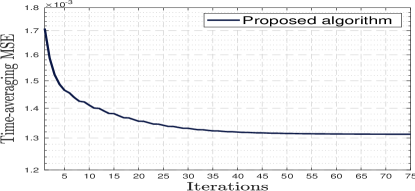
(a) Convergence behavior of Algorithm 1.

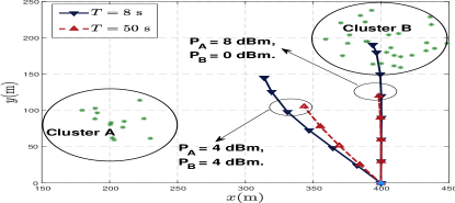
(b) Optimized UAV trajectories for different time horizons $T$.

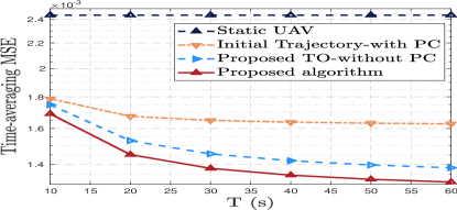
(c) The time-averaging MSE versus mission time.

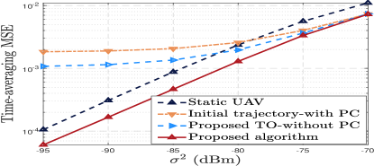
(d) The time-averaging MSE versus noise.

In summary, the overall algorithm adopts the BCD to solve the three sub-problems $\mathscr{P}_{1.1}$, $\mathscr{P}_{1.2}$, and $\mathscr{P}_{1.3}$ alternately in an iterative manner, which can return a suboptimal solution to problem $\mathscr{P}$. The details of the proposed algorithm are summarized in Algorithm 1. Problem $\mathscr{P}_{1.1}$ has a closed-form solution at each iteration. Furthermore, in each iteration, problem $\mathscr{P}_{1.2}$ is decoupled into $K$ QP problems (III-B) and problem $\mathscr{P}_{1.3}$ is approximated to the QCQP problem (24) by using the SCA technique. Since CVX invokes the interior-point method to solve problems (III-B) and (24), the total computational complexity of solving problems $\mathscr{P}_{1.2}$ and (24) are given by $O(KN^{2.5})$ and $O(K^{2.5}N^{2.5})$, respectively. Thus, in each iteration, the computational complexity of the proposed algorithm is given by $O(K^{2.5}N^{2.5})$.

III-E Initialization Scheme

In this subsection, we propose a low-complexity initialization scheme for the trajectory design and power control in Algorithm 1. Specifically, the initial power of each sensors is set be full power transmission, i.e., $p_{k}[n]=\bar{P}_{k}$, $\forall n$. Furthermore, the UAV first flies straight to the point above the geometric center at its maximum speed, then remains static at that point (if time permits), and finally flies at its maximum speed to reach its final location by the end of the last time slot. Note that if the UAV does not have sufficient time to reach the point above the ground node, it will turn at a certain midway point and then fly to the final location at the maximum speed.

IV Numerical Results

In this section, we provide numerical examples to demonstrate the effectiveness of the proposed algorithm. We consider a heterogeneous network, where $K=40$ sensors are separated into two clusters, i.e., $A$ with 13 sensors and $B$ with 27 sensors. The peak power budget of sensors in the cluster $A$ and $B$ are denoted as $P_{A}$ and $P_{B}$, respectively. The sensors in cluster $A$ and cluster $B$ are randomly and uniformly distributed in a circle centered at (200, 80) meter and (400, 200) meter with radius $50$ meters, respectively. The UAV is assumed to fly at a fixed altitude $H=100$ meters, which complies with the rule that all commercial UAV should not fly over 400 feet (122 meters) [21]. The maximum speed of the UAV is set as 30 m/s. $\delta$ is set as 0.2 s, which satisfies $\delta V_{\rm max}\ll H$. The receiver noise power is assumed to be $\sigma^{2}=-80$ dBm. Channel gain at reference distance is set as $\beta_{0}=-40$ dB. The average power budget is set as $\bar{P}_{k}=\frac{1}{2}P_{k}$. In addition, algorithm accuracy $\epsilon$ is set as $10^{-4}$.

In Fig. 2(a), we show the convergence behavior of the proposed algorithm when $T=50$ s and $P_{k}$ = 4 dBm for all $k$. Fig. 2(a) shows that the average MSE achieved by the proposed algorithm decreases quickly and converges in a few iterations, which demonstrates the effectiveness of the proposed algorithm for the joint UAV trajectory, power control, and denoising factors design.

In Fig. 2(b), we illustrate the trajectories obtained by the proposed algorithm under different periods $T$ and power budgets. Each trajectory is sampled every one second and the sampled points are marked with $\bigtriangleup$ by using the same colors as their corresponding trajectories. The user locations are marked by green $*$. The predetermined locations of UAV are blue $\star$. It is observed that when $T=8$ s, the UAV flies close to sensors from the initial location to the end of flight at the maximum speed. As $T$ increases, the UAV adaptively enlarges and adjusts its trajectory to move closer to the sensors. When time horizon $T$ is sufficiently large, i.e., $T=50$ s, the UAV first flies at the maximum speed to reach a certain location above the sensors, then remains stationary at this location as long as possible, and finally goes back to the initial location in an arc path at the maximum speed. The main reason for this result is that, in the AirComp setup, all the links’ channels are dependent on the UAV’s location at the same time slot. The closer the UAV flies to one particular sensor, the farther it is away from other sensors inevitably. As a result, these stationary locations strike an optimal balance enhancing all the links’ channels. In fact, this is also why the UAV follows an arc path rather than the straight path. Furthermore, for the diversified transmit power budgets, we observed that the controllable high-mobility UAV obtains different trajectories, thereby improving the AirComp performance.

Fig. 2(c) shows the time-averaging MSE versus different flight periods $T$ achieved by the following schemes when $P_{A}=P_{B}=4$ dBm: 1) Proposed algorithm, which is obtained by Algorithm 1; 2) Proposed TO without PC, where transmit power is obtained by full power transmission; 3) Initial Trajectory with PC, where UAV trajectory is obtained by the trajectory initialization in Section III-E; 4) Static UAV, where the UAV is placed at the predetermined position $(400,0,100)$ meter and remains static. First, it is observed that the average MSE achieved by all the schemes but static UAV decreases as $T$ increases by exploiting UAV mobility. Besides, the proposed algorithm has the smallest time-averaging MSE compared to other two benchmarks. Since the proposed algorithm dynamically strikes a balance between transmit power and all the links’ distances by fully exploiting the trajectory design and power control. The above results demonstrate the importance and necessity of the joint design.

Fig. 2(d) shows the robustness against noise of different algorithms when $P_{A}=4$ dBm, $P_{B}=8$ dBm, and $T=50$. It is observed that the time-averaging MSE achieved by all schemes increases as the noise power increasing while the proposed algorithm outperforms other three benchmarks throughout the whole noise regime. Interestingly, with low noise power, we observe that the performance gap between the proposed algorithm and only either power control or trajectory optimization schemes is very large. In all, it demonstrates that the proposed algorithm is robust to noise.

V Conclusion

In this paper, we considered a UAV-assisted AirComp system, where the UAV acting as an aerial BS is dispatched to aggregate the average function of distributed data. Therein, due to its controllable high-mobility and high-altitude, UAV can move sufficiently close to the sensors with LoS channels and adaptively strike a balance between communication distance and sensors’ diversified power budgets, which not only enhances the signal magnitude alignment but also mitigates the effect of noise. We studied the time-averaging MSE minimization problem, which jointly designs the UAV trajectory, denoising factors at UAV, and transmit power at sensors. An efficient iterative algorithm was further presented to solve the resulting non-convex optimization problem by applying the BCD and SCA techniques. Simulation results showed that significant performance gain and robustness of the proposed design as compared to other benchmarks as well as the ability of adaptive trajectory construction.

References

- [1] G. Zhu, J. Xu, and K. Huang, “Over-the-air computing for 6G - turning air into a computer,” arXiv, pp. 1–8, 2020.
- [2] K. Yang, T. Jiang, Y. Shi, and Z. Ding, “Federated learning via over-the-air computation,” IEEE Trans. Wireless Commun., vol. 19, no. 3, pp. 2022–2035, Mar. 2020.
- [3] T. Jiang and Y. Shi, “Over-the-air computation via intelligent reflecting surfaces,” in 2019 IEEE Glob. Commun. Conf., Waikoloa, Hawaii, USA, Dec. 2019.
- [4] X. Li, G. Zhu, Y. Gong, and K. Huang, “Wirelessly powered data aggregation for IoT via over-the-air function computation: Beamforming and power control,” IEEE Trans. Wireless Commun., vol. 18, no. 7, pp. 3437–3452, Jul. 2019.
- [5] J. Dong, Y. Shi, and Z. Ding, “Blind over-the-air computation and data fusion via provable wirtinger flow,” IEEE Trans. Signal Process., vol. 68, pp. 1136–1151, Jan. 2020.
- [6] K. B. Letaief, W. Chen, Y. Shi, J. Zhang, and Y. Zhang, “The roadmap to 6G: AI empowered wireless networks,” IEEE Commun. Mag., vol. 57, no. 8, pp. 84–90, aug 2019.
- [7] X. Cao, G. Zhu, J. Xu, and K. Huang, “Optimized power control for over-the-air computation in fading channels,” IEEE Trans. Wireless Commun., 2020, doi: 10.1109/TWC.2020.3012287.
- [8] L. Wang, H. Yang, J. Long, K. Wu, and J. Chen, “Enabling ultra-dense UAV-aided network with overlapped spectrum sharing: Potential and approaches,” IEEE Netw., vol. 32, no. 5, pp. 85–91, Sept. 2018.
- [9] L. Wang, Y. L. Che, J. Long, L. Duan, and K. Wu, “Multiple access mmWave design for UAV-aided 5G communications,” IEEE Wirel. Commun., vol. 26, no. 1, pp. 64–71, Feb. 2019.
- [10] Y. Zeng, Q. Wu, and R. Zhang, “Accessing from the sky: A tutorial on UAV communications for 5G and beyond,” Proc. IEEE, vol. 107, no. 12, pp. 2327–2375, Mar. 2019.
- [11] Y. Zeng and R. Zhang, “Energy-efficient UAV communication with trajectory optimization,” IEEE Trans. Wireless Commun., vol. 16, no. 6, pp. 3747–3760, Jun. 2017.
- [12] Q. Wu, Y. Zeng, and R. Zhang, “Joint trajectory and communication design for multi-UAV enabled wireless networks,” IEEE Trans. Wireless Commun., vol. 17, no. 3, pp. 2109–2121, Mar. 2018.
- [13] C. Zhan and Y. Zeng, “Completion time minimization for multi-UAV-enabled data collection,” IEEE Trans. Wireless Commun., vol. 18, no. 10, pp. 4859–4872, Oct. 2019.
- [14] C. Shen, T.-H. H. Chang, J. Gong, Y. Zeng, and R. Zhang, “Multi-UAV interference coordination via joint trajectory and power control,” IEEE Trans. Signal Process., vol. 68, pp. 843–858, Jan. 2020.
- [15] I. Qualcomm Technologies, LTE unmanned aircraft systems, San Diego, CA, USA, Trial report v.1.0.1, 2017.
- [16] U. Mengali and A. N. D’Andrea, Synchronization Techniques for Digital Receivers, New York, NY, USA: Springer, 1997.
- [17] Y. Xu and W. Yin, “A block coordinate descent method for regularized multiconvex optimization with applications to nonnegative tensor factorization and completion,” SIAM J. Imag. Sci., vol. 6, no. 3, pp. 1758–1789, 2013.
- [18] B. R. Marks and G. P. Wright, “A general inner approximation algorithm for nonconvex mathematical programs,” Operations research, vol. 26, no. 4, pp. 681–683, Jul. 1978.
- [19] M. Grant and S. Boyd, CVX: Matlab software for disciplined convex programming, version 2.1, Mar. 2014.
- [20] S. Boyd and L. Vandenberghe, Convex Optimization. Cambridge university press, 2004.
- [21] FAA, Summary of small unmanned aircraft rule, Washington, DC: Federal Aviation Administration, 2016.