Weak Signal Asymptotics for
Sequentially Randomized Experiments

Abstract

We use the lens of weak signal asymptotics to study a class of sequentially randomized experiments, including those that arise in solving multi-armed bandit problems. In an experiment with $n$ time steps, we let the mean reward gaps between actions scale to the order $1/\sqrt{n}$ so as to preserve the difficulty of the learning task as $n$ grows. In this regime, we show that the sample paths of a class of sequentially randomized experiments—adapted to this scaling regime and with arm selection probabilities that vary continuously with state—converge weakly to a diffusion limit, given as the solution to a stochastic differential equation. The diffusion limit enables us to derive refined, instance-specific characterization of stochastic dynamics, and to obtain several insights on the regret and belief evolution of a number of sequential experiments including Thompson sampling (but not UCB, which does not satisfy our continuity assumption). We show that all sequential experiments whose randomization probabilities have a Lipschitz-continuous dependence on the observed data suffer from sub-optimal regret performance when the reward gaps are relatively large. Conversely, we find that a version of Thompson sampling with an asymptotically uninformative prior variance achieves near-optimal instance-specific regret scaling, including with large reward gaps, but these good regret properties come at the cost of highly unstable posterior beliefs.

Keywords: Diffusion approximation, Multi-armed bandit, Thompson sampling.

1 Introduction

Sequential experiments, pioneered by Wald (1947) and Robbins (1952), involve collecting data over time using a design that adapts to past experience. Relative to classical randomized trials, they can effectively concentrate power on studying the most promising alternatives and save on costs by helping us avoid repeatedly taking sub-optimal actions. Such experiments have now become widely adopted for automated decision making; for example, Hill et al. (2017) show how sequential experiments can be used to optimize the layout and content of a website, while Ferreira et al. (2018) discuss applications to pricing and online revenue management.

Most existing research in sequential experimentation has focused on proving robust, worst-case guarantees. This has been motivated in a large part by automated decision making applications, such as website optimization and dynamic pricing, where it is common to run a large number of experiments in parallel while searching over a decision space. In these settings, it is important to use robust methods that perform reasonably well across all problem instances, so that they do not require frequent human oversight; see Bubeck and Cesa-Bianchi (2012) for a review and discussion.

More recently, however, there has been growing interest in settings where an agent performs a small number of high-stake sequential experiments: Athey et al. (2021) discuss the use of sequential experiments for learning better public health interventions, Caria et al. (2020) deploy them for targeting job search assistance for refugees, and Kasy and Teytelboym (2020) consider whom to test for an infectious disease in a setting where testing capacity is limited. In these applications where humans are likely to be closely monitoring and fine-tuning a small number of adaptive experiments, the relatively crude performance guarantees provided by worst-case analysis fall short in guiding the decision maker towards choosing the best policies. This gives rise to the need to develop a more refined, instance-specific understanding of the stochastic behavior of adaptive experiments. In particular, it would be of interest to understand:

• How to quantify the performance of an experiment in an instance-specific manner, that is, as a function of features of the environment in which the experiment is being conducted, such as gaps in mean rewards among different actions.

• Beyond just the mean, how to characterize the distributional properties of key performance measures of an adaptive experiment.

• How the behavior of adaptive experiments evolves over time, and what sample paths of actions taken by adaptive experiments look like.

Available worst-case-focused formal results, however, do not provide sharp answers to these questions that would apply broadly to popular algorithms for adaptive experimentation, including the ones used in the studies cited above. A central difficulty here is simply that sequential experiments induce intricate dependence patterns in the data that make sharp finite-sample analysis of their behavior exceedingly delicate.

In this paper, we introduce a new approach to studying sequential experiments based on black weak signal asymptotics. Specifically, we consider the behavior of adaptive experiments in a sequence of problems where, as the number of time steps $n$ grows to infinity, the gap between the mean rewards of different actions decays as $1/\sqrt{n}$. black We use this asymptotic regime to study the sequentially randomized Markov experiments, a general class of sequential experiments that includes several popular algorithms such as Thompson sampling (Thompson, 1933; Russo et al., 2018). black Our first result is that, under regularity conditions including continuity of how the arm selection probabilities vary with certain state variables, the sample paths of appropriately scaled sequentially randomized Markov experiments converge weakly to a diffusion limit characterized as the solution to a stochastic differential equation (SDE). We then show that this diffusion limit enables us to derive practical, instance-specific and distributional insights about the behavior of sequential experiments. The $1/\sqrt{n}$ arm gap scaling considered here is an important one. It can be thought of as a “moderate data” regime of sequential experimentation, where the problem’s inherent “signal strength,” expressed in terms of the mean reward gaps between the various actions, is not sufficiently stronge relative to sample size so as to make identifying the optimal action asymptotically trivial, but strong enough so that using a well designed policy is crucial as sub-optimal policies can lead to large regret.

In using diffusion approximation to obtain insights about the behavior of large, dynamic processes, our approach builds on a long tradition in operations research, especially in the context of queuing networks (Iglehart and Whitt, 1970; Harrison and Reiman, 1981; Reiman, 1984; Harrison, 1988; Glynn, 1990; Kelly and Laws, 1993; Gamarnik and Zeevi, 2006). A key insight from this line of work is that, by focusing on a heavy-traffic limit where server utilization approaches full capacity and wait times diverge, the behavior of a queuing network can be well approximated by a Brownian limit where, as argued by Kelly and Laws (1993), “important features of good control policies are displayed in sharpest relief.” Likewise, in our setting, we find that focusing on a scaling regime with small gaps in the mean rewards between the arms and long time horizons enables us to capture key aspects of sequential experiments in terms of a tractable diffusion approximation.

1.1 Overview of Main Results

Throughout this paper, we focus on the following $K$-armed setting, also known as a stochastic $K$-armed bandit. There is a sequence of decision points $i=1,\,2,\,\ldots,\,n$ at which an agent chooses which action $A_{i}\in\left\{1,\,\ldots,\,K\right\}$ to take and then observes a reward $Y_{i}\in\mathbb{R}$. Here, $Y_{i}$ is assumed to be drawn from a distribution $P_{A_{i}}$, where the action $A_{i}$ may depend on past observations, and is conditionally independent from all other aspects of the system given the realization of $A_{i}$. Our goal is to use diffusion approximation to characterize the behavior of $K$-armed bandits in terms of a number of metrics, including regret

$$R^{n}=n\sup_{1\leq k\leq K}\left\{\mu_{k}\right\}-\mathbb{E}\left[\sum_{i=1}^{n}\mu_{A_{i}}\right],\ \ \ \ \mu_{k}=\mathbb{E}_{P_{k}}\left[Y\right],$$ (1.1)

i.e., the shortfall in rewards incurred by the bandit algorithm relative to always taking the best action. Unless otherwise specified, we will use “arm gap” as a short-hand for the gap between the mean rewards associated with the two best arms.

The first part of our paper, Section 2, black introduces a weak signal scaling regime for the reward distributions, where arm gaps become small as the sample size of the experiment increases. We then establish that for a broad class of sequential experiments, which we refer to as sequentially randomized Markov experiments, the system dynamics converge to a diffusion limit under this weak signal asymptotic regime. This result applies to a wide variety of adaptive experimentation rules arising in statistics, machine learning and behavioral economics black including Thompson sampling (see Examples 1–4 given below). We also find that this diffusion limit can be characterized using random time-change applied to a Brownian motion, which enables much of our subsequent theoretical analysis. black Throughout our analysis, we assume that the arm selection probabilities in the sequentially randomized Markov experiments we consider vary continuously with relevant state variables. We provide convergence results for both when the limiting sampling function is Lipschitz continuous, and when it is continuous but non-Lipschitz; black however, our results do not apply to bandit algorithms with a discontinuous deterministic component, such as UCB or $\varepsilon$-greedy.

In the second part of the paper, we use our diffusion limit to obtain insights on the regret performance of a host of practical adaptive experiments. First, we turn our attention to the class of sequentially randomized experiments that admit an asymptotically Lipschitz limiting sampling function, which includes among other examples the popular Gaussian Thompson sampling algorithm with an asymptotically proper prior. These experiments tend to have favorable stability properties, making them less likely to overreact to the observed data and their dynamics more amenable to analysis. Surprisingly, we prove in Section 4.1 that any experiment with an asymptotically Lipschitz sampling function necessarily has poor regret performance: in the diffusion limit, the scaled regret of any such experiment remains bounded from below as the arm gap gets large, whereas the corresponding minimax risk goes to zero. Our result thus shows that the benefits of stability of Lipschitz sampling come at the expense of regret performance, as the algorithm cannot not abandon a bad action quickly enough in the early stages of the experiment.

As a counterpoint to the first finding, our next result demonstrates that, in a two-armed setting, we can achieve nearly instance-optimal regret by adopting a non-Lipschitz sampling function. We examine an “undersmoothed” version of the Thompson sampling algorithm where the agent uses an asymptotically uninformative prior distribution. We prove in Section 4.2 that the regret of undersmoothed Thompson sampling not only vanishes as the arm gap grows, but does so at a rate that is nearly optimal in comparison to known instance-specific lower bounds (Mannor and Tsitsiklis, 2004), a sharp contrast to the negative result on Lipschitz sampling described earlier. This is, to the best of our knowledge, the first result to highlight good instance-dependent regret properties for Thompson sampling in the moderate signal-to-noise regime (i.e., with $1/\sqrt{n}$-scale arm gaps).

Finally, we leverage the diffusion limit to obtain insights on distributional properties of sample paths in an adaptive experiment. We prove in Section 5 that, for a family of one-armed problems, experiments with a “sensitive” sampling function—ones that respond quickly to observed data—will be highly unstable, where the sampling probability of choosing the optimal arm can swing wildly between very large to the very small, and that this can happen even with very large arm gaps. This result covers undersmoothed Thompson sampling, in which case our analysis implies large swings in its posterior beliefs. This finding complements our regret analysis to render a more complete and nuanced picture, suggesting that an agent may have to face a fundamental trade-off between achieving optimal regret and maintaining a relatively stable sample path.

On the methodological front, our work introduces new tools to the study of adaptive experiments. We show weak convergence to the diffusion limit for sequentially randomized Markov experiments using the martingale framework developed by Stroock and Varadhan (2007), which hinges on showing that an appropriately scaled generator of the discrete-time Markov process converges to the infinitesimal generator of the diffusion process. Our analysis of the regret profiles of Thompson sampling under the weak signal scaling relies on novel proof arguments that heavily exploit properties of Brownian motion, such as the Law of Iterated Logarithm.

1.2 Related Work

The multi-armed bandit problem is a popular framework for studying sequential experimentation; see Bubeck and Cesa-Bianchi (2012) for a broad discussion focused on bounds on the regret (1.1). An early landmark result in this setting is due to Lai and Robbins (1985), who showed that given any fixed set of arms $\left\{P_{k}\right\}_{k=1}^{K}$, a well-designed sequential algorithm can achieve regret that scales logarithmically with the number $n$ of time steps considered, i.e., $R^{n}=\mathcal{O}_{P}(\log(n))$. Meanwhile, given any fixed time horizon $n$, it is possible to choose probability distributions $\left\{P_{k}\right\}_{k=1}^{K}$ such that the expected regret $\mathbb{E}\left[R^{n}\right]$ of any sequential algorithm is lower-bounded to order $\sqrt{Kn}$ (Auer et al., 2002). It is worth-noting that the problem instance that achieves the $\sqrt{Kn}$ regret lower bound in Auer et al. (2002) involves the same mean reward scaling as we use for our diffusion limit, suggesting that the black weak signal scaling proposed here captures the behavior of the most challenging (and thus potentially most interesting) sub-family of learning tasks.

Thompson sampling (Thompson, 1933; Russo et al., 2018) has gained considerable popularity in recent years thanks to its simplicity and impressive empirical performance (Chapelle and Li, 2011). Regret bounds for Thompson sampling have been established in the frequentist (Agrawal and Goyal, 2017; Kaufmann et al., 2012) and Bayesian (Bubeck and Liu, 2014; Lattimore and Szepesvári, 2019; Russo and Van Roy, 2016) settings; the setup here belongs to the first category. None of the existing instance-dependent regret bounds, however, appear to have sufficient precision to yield meaningful characterization in our regime. For example, the instance-dependent upper bound in Agrawal and Goyal (2017) contains a constant to the order of $1/\Delta^{4}$, where $\Delta$ is the gap in mean reward between optimal and sub-optimal arms. This would thus lead to a trivial bound of $\mathcal{O}(n^{2})$ in our regime, where mean rewards scale as $1/\sqrt{n}$. Furthermore, many of the existing bounds also require delicate assumptions on the reward distributions (e.g., bounded support). In contrast, the black weak signal asymptotics adopted in this paper are universal in the sense that they automatically allow us to obtain approximations for a much wider range of reward distributions, requiring only a bounded fourth moment.

Our choice of the weak signal scaling and the ensuing diffusion limit are motivated by insights from both queueing theory and statistics. The scaling plays a prominent role in heavy-traffic diffusion approximation in queueing networks (Gamarnik and Zeevi, 2006; Harrison and Reiman, 1981; Reiman, 1984); in particular, Harrison (1988) uses diffusion approximation to study a dynamic control problem. Here, one considers a sequence of queueing systems in which the excessive service capacity, defined as the difference between arrival rate and service capacity, decays as $1/\sqrt{T}$, where $T$ is the time horizon. Under this asymptotic regime, it is shown that suitably scaled queue-length and workload processes converge to reflected Brownian motion. Like in our problem, the diffusion regime here is helpful because it captures the most challenging problem instances, where the system is at once stable and exhibiting non-trivial performance variability. See also Glynn (1990) for an excellent survey for the use of diffusion approximation in operations research.

The black weak signal asymptotics are further inspired by a recurring insight from statistics that, in order for asymptotic analysis to yield a normal limit that can be used for finite-sample insight, we need to appropriately down-scale the arm gap as the sample size gets large. One concrete example of this phenomenon arises when we seek to learn optimal decision rules from (quasi-)experimental data. Here, in general, optimal behavior involves regret that decays as $1/\sqrt{n}$ with the sample size (Athey and Wager, 2021; Hirano and Porter, 2009; Kitagawa and Tetenov, 2018); however, this worst-case regret is only achieved if we let effect sizes decay as $1/\sqrt{n}$. For any fixed sampling design, it’s possible to achieve faster than $1/\sqrt{n}$ rates asymptotically (Luedtke and Chambaz, 2020).

Our work is broadly related to work on adaptive learning and experimentation in the statistics and operations research literatures. The seminal work of Chernoff (1959) studies how to adaptively choose from a menu of available experiments for hypothesis testing, and the main result consists of a dynamic experiment that achieves the asymptotic optimal rate of convergence to the true hypothesis as the number of samples grows. A number of papers expand upon this framework, including Naghshvar and Javidi (2013) who drive a range of refinements and extensions on the minimax bounds, Russo (2020) who adapts the algorithm for best-arm identification, and Massoulié and Xu (2018) who consider simultaneous experiments run in a resource-limited setting. The asymptotic regime considered in this line of work is different from ours: They focus on the large-deviation regime where the problem instance stays fixed while the number of samples grows to infinity, whereas we consider the black weak signal regime where the arm gap decreases along with the sample size. Another distinction is that this literature tends to treat what has become known as the post-experiment simple regret, where the agent’s cost is determined by any error incurred in declaring the incorrect hypothesis after the completion of the experiment, rather than the in-experiment regret accrued due to using sub-optimal arms during the experiment.

There are some existing results where diffusion-based analysis has been used for action selection and optimal stopping in sequential experiments. Some of the earlier studies assume randomization is fixed over the horizon (Siegmund, 1985). In contrast, in our multi-armed bandit setting the probabilities in the randomization depend on the history which creates a qualitatively different limit object. Chick and Gans (2009) consider optimal stopping in ranking and selection where the agent runs a sequence of experiments to determine which action carries the maximum expected payoff. They then apply diffusion approximation to the resulting Bellman equation and derive tractable structural results for simple cases. Araman and Caldentey (2021) study an adaptive optimal stopping problem with a binary hypothesis and use the diffusion limit to derive insights on how and when the agent should act, as well as the optimal choice of experiments. Wang and Zenios (2020) consider a model similar to Araman and Caldentey (2021) in the context of adaptive clinical trials, with the additional feature that the experiments can have different costs. Harrison and Sunar (2015) use diffusion approximation to study an optimal stopping problem with a binary hypothesis when a firm decides between making an investment versus taking further learning actions to gather more information. The approaches taken in these papers are however different from ours. First, they tend to focus on discrete (and often binary) hypothesis testing whereas we study multi-armed experiments with continuously-valued mean rewards. Second, the optimal stopping formulation is centered around the expected cost incurred by a one-shot, post-experiment action choice, in contrast to the in-experiment regret analyzed here. Third, most of these papers focus on solving exactly, or approximately, the Bayesian Bellman-optimal decision rule based on dynamic programming, whereas we are more interested in characterizing the dynamics of a range of heuristic policies, such as Thompson sampling, which are used in practice when the Bayesian priors of the model parameters are unknown or the agent operates under a frequentist, instance-specific performance mandate. Lastly, in this literature, diffusion approximation is sometimes evoked directly or introduced as a modeling assumption without a proof of convergence (e.g., Chick and Gans, 2009; Harrison and Sunar, 2015).

Finally, after we posted a first version of this paper, a number of authors have disseminated work that intersects with our main result. In the special case of Thompson sampling, Fan and Glynn (2021) derive the diffusion limit given in Theorems 1 and 3 using a different proof technique from us: As discussed further in Appendix A, we derive the diffusion limit by studying the asymptotic behavior of the Markov chain associated with our sequential experiments following Stroock and Varadhan (2007), whereas Fan and Glynn (2021) develop a direct argument based on the continuous mapping theorem. Meanwhile, Hirano and Porter (2021) extend the “limits of experiments” analysis pioneered by Le Cam (1972) to discrete-time, batched sequential experiments. The limits of experiments paradigm also involves a $1/\sqrt{n}$-scale local parametrization, and their results can be applied to sequentially randomized Markov experiments whose the randomization probabilities only change at a finite set of pre-specified times. Both Fan and Glynn (2021) and Hirano and Porter (2021) are based on research developed independently from ours.

2 Asymptotics for K-Armed Sequential Experiments

As discussed above, the first goal of this paper is to establish a diffusion limit for a class of sequential experiments. To this end, we first introduce a broad class of sequential experimentation schemes in Section 2.1, which we refer to as sequentially randomized Markov experiments. We describe a black weak signal scaling for sequential experiments in Section 2.2; then, in Section 3, we establish conditions under which—in this limit—sample paths of sequentially randomized Markov experiments converge weakly to the solution of a stochastic differential equation.

Throughout our analysis, we work within the following $K$-armed model. This model captures a number of interesting problems and is widely used in the literature (e.g., Bubeck and Cesa-Bianchi, 2012; Lai and Robbins, 1985). However, we note that it does rule out some phenomena that may arise in applications; for example, we do not allow for distribution shift in the reward distribution of a given arm over time, and we do not allow for long-term consequences of actions, i.e., an action taken in period $i$ cannot affect arm-specific period-$i^{\prime}$ reward distributions for any $i^{\prime}>i$. Extending our asymptotic analysis to allow for distribution shift or long-term effects would be of considerable interest, but we do not pursue this line of investigation in the present paper.

Definition 1 (Stochastic $K$-Armed Bandit).

A stochastic $K$-armed bandit is characterized by time horizon $n$ and a set of $K$ reward distributions $P_{k}$ for $k=1,\,\ldots,\,K$. At each decision points $i=1,\,2,\,\ldots,\,n$, an agent chooses which action $A_{i}\in\left\{1,\,\ldots,\,K\right\}$ to take and then observes a reward $Y_{i}\in\mathbb{R}$. The action $A_{i}$ is a random variable that is measurable with respect to the observed history $\left\{A_{i^{\prime}},\,Y_{i^{\prime}}\right\}_{i^{\prime}=1}^{i-1}$. Then, conditionally on the chosen action $A_{i}$, the reward $Y_{i}$ is drawn from the distribution $P_{A_{i}}$, independently from the observed history.

2.1 Sequentially Randomized Markov Experiments

In the interest of generality, we state our main results in the context of sequentially randomized experiments whose sampling probabilities depend on past observations only through the state variables

$$Q_{k,i}=\sum_{j=1}^{i}\mathbf{1}\left(\left\{A_{j}=k\right\}\right),\quad S_{k,i}=\sum_{j=1}^{i}\mathbf{1}\left(\left\{A_{j}=k\right\}\right)Y_{j},$$ (2.1)

where $Q_{k,i}$ counts the cumulative number of times arm $k$ has been chosen by the time we collect the $i$-th sample, and $S_{k,i}$ measures its cumulative reward. When useful, we use the convention $Q_{k,0}=S_{k,0}=0$. Working with this class of algorithms, which we refer to as sequentially randomized Markov experiments, enables us to state results that cover many popular ways of running sequential experiments without needing to derive specialized analyses for each of them.

Definition 2 (Sequentially Randomized Markov Experiment).

A $K$-armed sequentially randomized Markov experiment chooses the $i$-th action $A_{i}$ by taking a draw from a distribution

$$A_{i}\,\big{|}\,\left\{A_{1},\,Y_{1},\,\ldots,\,A_{i-1},\,Y_{i-1}\right\}\sim\operatorname{Multinomial}(\pi_{i}),$$ (2.2)

where the sampling probabilities are computed using a measurable sampling function $\psi$,

$$\psi:\mathbb{R}^{K}\times\mathbb{R}^{K}\rightarrow\mathbf{\Delta}^{K},\ \ \ \pi_{i}=\psi\left(Q_{i-1},S_{i-1}\right),$$ (2.3)

where $(Q_{i-1})=(Q_{k,i-1})_{k=1,\ldots,K},S_{i-1}=(S_{k,i-1})_{k=1,\ldots,K}$, and $\mathbf{\Delta}^{K}$ is the $K$-dimensional unit simplex.

Remark 1 (Capturing Time Dependence).

It is useful to note that the family of experiments described in Definition 2 contains those algorithms whose sampling probabilities may depend on the time period, $i$. This is captured through the fact that $\sum_{k}Q_{i,k}=i$, that is, the time period $i$ can be simply read off by calculating the $L_{1}$ norm of the vector $Q_{i}$.

We now examine several examples of popular algorithms that fit under the sequentially randomized Markov experiment framework.

Example 1.

A greedy agent may be tempted to always pull the arm with the highest apparent mean, $S_{i,k}/Q_{i,k}$; however, this strategy may fail to experiment enough and prematurely discard good arms due to early unlucky draws. A tempered greedy algorithm instead chooses arm $k$ with probability:

$$\pi_{i,k}=\exp\left[\alpha\frac{S_{k,i}}{Q_{k,i}+c}\right]\,\bigg{/}\,\sum_{l=1}^{K}\exp\left[\alpha\frac{S_{l,i}}{Q_{l,i}+c}\right],$$ (2.4)

where $\alpha,\,c>0$ are tuning parameters that serve to govern the strength of the extent to which the agent focuses on the greedy choice and to protect against division by zero, respectively. The selection choices (2.4) satisfy (2.3) and thus Definition 2 by construction.

Example 2.

Similar learning dynamics arise in human psychology and behavioral economics where an agent chooses future actions with a bias towards those that have accrued higher (un-normalized) cumulative reward (Erev and Roth, 1998; Xu and Yun, 2020). A popular example, known as Luce’s rule (Luce, 1959), uses sampling probabilities

$$\pi_{i,k}=(S_{k,i}\vee\alpha)\bigg{/}\sum_{l=1}^{K}(S_{l,i}\vee\alpha),$$ (2.5)

where $\alpha\geq 0$ is a tuning parameter governing the amount of baseline exploration. More generally, the agent may ascribe to arm $k$ a weight $f(S_{k,i})$, where $f$ is a non-negative potential function, and sample actions with probabilities proportional to the weights. The decision rule in (2.5) only depends on $S$ and thus satisfies (2.3).

Example 3.

Thompson sampling is a popular Bayesian heuristic for running sequential experiments (Thompson, 1933). In Thompson sampling an agent starts with a prior belief distribution $G_{0}$ on the reward distributions $\left\{P_{k}\right\}_{k=1}^{K}$. Then, at each step $i$, the agent samples a reward distribution from their posterior belief $G_{i-1}$, pulls the optimal arm that has the highest mean according to this sampled distribution, and uses the resulting realized reward to update the posterior $G_{i}$ using Bayes’ rule. The motivation behind Thompson sampling is that it quickly converges to pulling the best arm, and thus achieves low regret (Agrawal and Goyal, 2017; Chapelle and Li, 2011). Thompson sampling does not always satisfy Definition 2. However, widely used modeling choices involving exponential families for the $\left\{P_{k}\right\}_{k=1}^{K}$ and conjugate priors for $G_{0}$ result in these posterior probabilities $\rho_{k,i}$ satisfying the sufficiency condition (2.3) (Russo et al., 2018), in which case Thompson sampling yields a sequentially randomized Markov experiment in the sense of Definition 2.

In this paper, we will focus on one of the most widely used variants of this design, Gaussian Thompson sampling. In this setting the agent models $P_{k}^{n}$ as a Gaussian distribution with (unknown) mean $\mu_{k}^{n}$ and (known) variance $\sigma_{k}^{2}$, and sets the prior distribution $G_{0}$ on the mean rewards $\mu_{k}^{n}$ of each arm to be Gaussian with mean 0 and variance $(\nu^{n})^{2}I_{K\times K}$. (Note that the Gaussian assumption only affects the behavior of the agent’s algorithm; the actual reward distributions are not necessarily Gaussian.) The posterior sampling step described above then takes on a simple form in this model: For each step $i=1,\,\ldots,\,n$ we generate draws

$$\begin{split}&\tilde{\mu}_{k}^{i}\,\big{|}\,G_{k,i}^{n}\sim\mathcal{N}\left(\frac{\sigma_{k}^{-2}S_{k,i}}{\sigma_{k}^{-2}Q_{k,i}+\left(\nu^{n}\right)^{-2}},\ \ \frac{1}{\sigma_{k}^{-2}Q_{k,i}+\left(\nu^{n}\right)^{-2}}\right),\end{split}$$ (2.6)

and then pull the arm corresponding to the largest $\tilde{\mu}_{k}^{i}$. This sampling step clearly corresponds to a sequentially randomized Markov experiment. Formally, here,

$$\psi\left(Q_{i},\,S_{i}\right)=\Pi^{\sup}\left(Q_{i},\,S_{i},;\,\sigma,\,\nu^{n}\right),$$ (2.7)

where $\Pi^{\sup}_{k}(q,\,s;\,\sigma,\,\nu^{n})$ denotes the probability that the $k$-th draw $\tilde{\mu}_{k}^{i}$ from (2.6) is largest, with $S_{l,i}=s_{l}$ and $Q_{l,i}=s_{l}$ for all $l=1,\,\ldots,\,K$.

Example 4.

Exploration sampling is a variant of Thompson sampling where, using notation from the above example, the agent pulls each arm with probability $\pi_{k,i}=\rho_{k,i}(1-\rho_{k,i})/\sum_{l=1}^{K}\rho_{l,i}(1-\rho_{l,i})$ instead of $\pi_{k,i}=\rho_{k,i}$ (Kasy and Sautmann, 2021). Exploration sampling is preferred to Thompson sampling when the analyst is more interested in identifying the best arm than simply achieving low regret (Kasy and Sautmann, 2021; Russo, 2020). Exploration sampling satisfies Definition 2 under the same conditions as Thompson sampling.

Example 5.

The Exp3 algorithm, proposed by Auer et al. (2002), uses sampling probabilities

$$\pi_{i,k}=\exp\left[\alpha\,\sum_{j=1}^{i-1}\frac{\mathbf{1}\left(\left\{A_{j}=k\right\}\right)Y_{j}}{\pi_{j,k}}\right]\,\bigg{/}\,\sum_{l=1}^{K}\exp\left[\alpha\,\sum_{j=1}^{i-1}\frac{\mathbf{1}\left(\left\{A_{j}=l\right\}\right)Y_{j}}{\pi_{j,l}}\right],$$ (2.8)

where again $\alpha>0$ is a tuning parameter. The advantage of Exp3 is that it can be shown to achieve low regret even when the underlying distributions $\left\{P_{k}\right\}_{k=1}^{K}$ may be non-stationary and change arbitrarily across samples. The sampling probabilities (2.8) do not satisfy (2.3), and so the Exp3 algorithm is not covered by the results given in this paper; however, it is plausible that a natural extension of our approach to non-stationary problems could be made accommodate it. We leave a discussion of non-stationary problems to future work.

2.2 A black Weak Signal Scaling

Next, we describe a sequence of experiments, indexed by $n$, and how the dynamics associated with these experiments converge to a diffusion limit under appropriate scaling. In order for behaviors of sequentially randomized Markov experiments to admit a limit distribution, we will require both the reward distributions $P^{n}$ and sampling functions $\psi^{n}$ used in the $n$-th experiment to converge in an appropriate sense. First, we will assume that reward distributions satisfy the following black weak signal scaling. Unless otherwise stated, all reward distributions are assumed to be in this scaling regime for the remainder of the paper.

Definition 3 (black Weak Signal Regime of Reward Distributions).

Consider a sequence of $K$-armed stochastic bandit problems in the sense of Definition 1, with reward distributions $\{P^{n}_{k}\}_{k,n\in\mathbb{N}}$. We say that this sequence resides in the black weak signal regime if there exist $\mu,\sigma\in\mathbb{R}_{+}^{K}$ such that

$$\lim_{n\rightarrow\infty}\sqrt{n}\mu_{k}^{n}=\mu_{k},\ \ \ \ \ \ \ \ \ \lim_{n\rightarrow\infty}\left(\sigma_{k}^{n}\right)^{2}=\sigma_{k}^{2},$$ (2.9)

where $\mu_{k}^{n}=\mathbb{E}_{P^{n}_{k}}\left[Y\right]$ and $\left(\sigma_{k}^{n}\right)^{2}=\operatorname{Var}_{P^{n}_{k}}\left[Y\right]$.

A simple sequence of models in the black weak signal regime is the Gaussian model where rewards from arm-$k$ in the $n$-th system are normally distributed, $Y_{i}\,\big{|}\,A_{i}=k\sim\mathcal{N}(\mu^{n}_{k},\sigma^{2}_{k})$, where $\mu^{n}_{k}\sqrt{n}\to\mu_{k}$ as $n$ grows whereas the variance $\sigma^{2}_{k}>0$ remains fixed. We can also construct a Bernoulli model in the black weak signal regime by considering centered rewards. If $Y_{i}=Z_{i}-\zeta_{0}$ where $Z_{i}\,\big{|}\,A_{i}=k\sim\text{Bernoulli}(\zeta_{k}^{n})$ and $\sqrt{n}(\zeta_{k}^{n}-\zeta_{0})\to\delta_{k}$, then we are in the diffusion regime with $\mu_{k}=\delta_{k}$ and $\sigma_{k}^{2}=\zeta_{0}(1-\zeta_{0})$. We discuss the further role of centering in our setting in Remark 2 below.

Next, we require the sequence of sampling functions to converge in an appropriate sense. As discussed further below, the natural scaling of the the $Q_{k,i}$ and $S_{k,i}$ state variables defined in (2.1) is

$$Q_{k,i}^{n}=\frac{1}{n}\sum_{j=1}^{i}\mathbf{1}\left(\left\{A_{j}=k\right\}\right),\quad S_{k,i}^{n}=\frac{1}{\sqrt{n}}\sum_{j=1}^{i}\mathbf{1}\left(\left\{A_{j}=k\right\}\right)Y_{j}.$$ (2.10)

We then say that a sequence of sampling functions $\psi^{n}$ is convergent if it respects this scaling.

Definition 4 (Convergent Sampling Function).

Writing sampling functions in a scale-adapted way as follows,

$$\bar{\psi}^{n}(q,s)=\psi^{n}\left(nq,\sqrt{n}s\right),\quad q\in[0,\,1]^{K},s\in\mathbb{R}^{K},$$ (2.11)

we say that a sequence of sampling functions $\psi^{n}$ satisfying (2.3) is convergent if

$$\bar{\psi}^{n}\stackrel{{\scriptstyle n\to\infty}}{{\longrightarrow}}\psi$$ (2.12)

uniformly over all compact subsets of $[0,\,1]^{K}\times\mathbb{R}^{K}$, for a limiting sampling function $\psi$.

When using our results in applications, one key practical consideration is in understanding conditions under which it is natural to consider a sequence of sampling functions $\psi^{n}$ that is convergent in the sense of Definition 4. We here revisit some of our earlier examples in the context of these scaling considerations.

Example 0 (continued).

The tempered greedy method can immediately be seen to be convergent, provided we use a sequence of tuning parameters $\alpha_{n}$ and $c_{n}$ satisfying $\lim_{n\rightarrow\infty}\sqrt{n}\alpha_{n}=\alpha$ and $\lim_{n\rightarrow\infty}nc_{n}=c$ for some $\alpha,\,c\in\mathbb{R}_{+}$, resulting in a limiting sampling function

$$\psi_{k}\left(q,s\right)=\exp\left[\alpha\frac{s_{k}}{q_{k}+c}\right]\,\bigg{/}\,\sum_{l=1}^{K}\exp\left[\alpha\frac{s_{l}}{q_{l}+c}\right].$$ (2.13)

For tempered greedy sampling to be interesting, we in general want the limit $\alpha$ to be strictly positive, else the claimed diffusion limit (3.1) will be trivial. Conversely, for the second parameter, both the limits $c>0$ and $c=0$ may be interesting, but working in the $c=0$ limit may lead to additional technical challenges due to us getting very close to taking an ill-conditioned ratio.

Example 0 (continued).

Luce’s rule is convergent whenever $\sqrt{n}\alpha_{n}\to\alpha>0$.

Example 0 (continued).

There are two ways to make Gaussian Thompson sampling (2.6) convergent. The first is to scale the prior variance $(\nu^{n})^{2}$ in a manner that matches the order-of-magnitude of the mean rewards in the black weak signal regime. Since the mean reward scales on the order of $1/\sqrt{n}$, this would amount to having

$$\lim_{n\rightarrow\infty}(\nu^{n})^{-2}/n=c>0.$$ (2.14)

With this scaling and using notation from (2.7), we can check the probability of the $k$-th posterior sample being largest satisfies

$$\begin{split}\psi^{n}(nq,\,\sqrt{n}s)&=\Pi^{\sup}(nq,\,\sqrt{n}s;\,\sigma^{2},\,\nu^{-2})\\ &=\Pi^{\sup}(q,\,s;\,\sigma^{2},\,\nu^{-2}/n)\to\Pi^{\sup}(q,\,s;\,\sigma^{2},\,c),\end{split}$$ (2.15)

and thus the induced sampling functions are in fact convergent. The second is to scale the prior variance such that

$$\lim_{n\rightarrow\infty}(\nu^{n})^{-2}/n=0,\ \ \ \ \ \psi^{n}(nq,\,\sqrt{n}s)\to\Pi^{\sup}(q,\,s;\,\sigma^{2},\,0),$$ (2.16)

in which case the prior is asymptotically uninformative about diffusion scale mean rewards. We will again see that the (2.14) and (2.16) lead to markedly different statistical properties; we refer to the former as smoothed Thompson sampling and to the latter as undersmoothed Thompson sampling.

Example 0 (continued).

As before, exploration sampling is convergent whenever the associated Thompson sampling rule is.

Remark 2 (Non-Zero Mean Rewards).

The scaling condition in Definition 3 implies that, in large samples, all arms have roughly zero rewards on average, i.e., $\lim_{n\rightarrow\infty}\mu_{k}^{n}=0$. In some applications, however, it may be more natural to consider a local expansion around non-zero mean rewards, where

$$\lim_{n\rightarrow\infty}\sqrt{n}\left(\mu_{k}^{n}-\mu_{0}\right)=\delta_{k}$$ (2.17)

for some potentially non-zero $\mu_{0}\neq 0$ and $\delta\in\mathbb{R}^{K}$. In our general results, we focus on the setting from Definition 3; however, we note that, when applied to any translation-invariant algorithm (i.e., a sequential experiment whose sampling function is invariant to adding a fixed offset to all rewards), any results proven under the setting of Definition 3 will also apply under (2.17). In Section 4.2, we will use this fact when studying a translation-invariant Thompson sampling algorithm.

3 Convergence to a Diffusion Limit under black Weak Signal Scaling

We are now ready to state our first main result: Given a sequence of reward distributions satisfying (2.9) and under a number of regularity conditions discussed further below, the sample paths of the scaled statistics $Q_{k,i}^{n}$ and $S_{k,i}^{n}$ of a sequentially randomized Markov experiments with convergent sampling functions converge in distribution to the solution to a stochastic differential equation

$$\begin{split}&dQ_{k,t}=\psi_{k}\!\left(Q_{t},S_{t}\right)dt,\\ &dS_{k,t}=\mu_{k}\,\psi_{k}\!\left(Q_{t},S_{t}\right)dt+\sigma_{k}\sqrt{\psi_{k}\!\left(Q_{t},S_{t}\right)}dB_{k,t},\end{split}$$ (3.1)

where $B_{\cdot,\,t}$ is a standard $K$-dimensional Brownian motion, $\mu_{k}$ and $\sigma_{k}$ and the mean and variance parameters given in (2.9), and the time variable $t\in[0,\,1]$ approximates the ratio $i/n$. A formal statement is given in Theorem 1.

We will consider separately two cases depending on whether the limiting sampling function, $\psi$, is Lipschitz-continuous, or continuous but non-Lipschitz. We begin with the case where $\psi$ is Lipschitz, which allows us to obtain stronger convergence guarantees, before extending the results to the non-Lipschitz case. As will be discussed further below, tempered greedy and Thompson sampling with $c>0$ as well as Luce’s rule are all examples with Lipschitz limiting sampling functions, while tempered greedy and Thompson sampling with $c=0$ are examples of the non-Lipschitz case.

Remark 3.

In our current analysis, we do not consider cases where the limiting sampling function $\psi$ is not continuous with respect to the underlying state $(Q,S)$. Considering the discontinuous case could also be of interest, as there are a number of bandit algorithms—including upper-confidence bound (UCB) and $\epsilon$-greedy algorithms—that are consistent with Definition 2 but with sampling functions $\psi$ that have sharp cutoffs.

Remark 4.

We generally assume that the reward variances are known and do not consider the problem of estimating them. This is because, black under the weak signal scaling, the arm variances stay constant while the number of samples scales, and therefore the variances can be accurately estimated.

3.1 Lipschitz Limiting Sampling Functions

Given any Lipschitz sampling functions, we will show that a suitably scaled version of the process $(Q^{n}_{i},S^{n}_{i})$ converges to an Itô diffusion process. Define $\widebar{Q}^{n}_{t}$ to be the linear interpolation of $Q^{n}_{\lfloor tn\rfloor}$,

$$\widebar{Q}^{n}_{k,t}=(1-tn+\lfloor tn\rfloor)Q^{n}_{k,{\lfloor tn\rfloor}}+(tn-\lfloor tn\rfloor)Q^{n}_{k,\lfloor tn\rfloor+1},\quad t\in[0,1],k=1,\ldots,K,$$ (3.2)

and define the process $\widebar{S}^{n}_{t}$ analogously. Here, $n$ is the total number of samples in the experiment, and the continuous index $t$ can be thought of as the fraction of total samples collected up to a certain point. For instance, $(\widebar{Q}^{n}_{0.5},\widebar{S}^{n}_{0.5})$ can be viewed as the state of the system at the mid-point of an experiment.

Let $\mathcal{C}$ be the space of continuous functions $[0,1]\mapsto\mathbb{R}^{2K}$ equipped with the uniform metric: $d(x,y)=\sup_{t\in[0,1]}|x(t)-y(t)|$, $x,y\in\mathcal{C}$. We have the following result; the proof is given in Section A.1.

Theorem 1.

Fix $K\in\mathbb{N}$, $\mu\in\mathbb{R}^{K}$ and $\sigma\in\mathbb{R}_{+}^{K}$. Suppose that we have a sequence of $K$-armed bandit problems as in Definition 1, whose reward distributions $\{P^{n}_{k}\}_{k,n\in\mathbb{N}}$ reside in the black weak signal regime as per Definition 3 and admit fourth moments that are uniformly bounded across $k$ and $n$. Suppose that we have a convergent sequence of sequentially randomized Markov experiments following Definitions 2 and 4. Suppose furthermore that the limit sampling function $\psi$ is Lipschitz-continuous, and $(\widebar{Q}^{n}_{0},\widebar{S}^{n}_{0})=0$. Then, as $n\rightarrow\infty$, $(\widebar{Q}^{n}_{t},\widebar{S}^{n}_{t})_{t\in[0,1]}$ converges weakly to $(Q_{t},S_{t})_{t\in[0,1]}\in\mathcal{C}$, which is the unique solution to black the stochastic differential equation (3.1) over $t\in[0,1]$, where $(Q_{0},S_{0})=0$ and $B_{t}$ is a standard Brownian motion in $\mathbb{R}^{K}$ with independent components. Furthermore,

$$\lim_{n\rightarrow\infty}\mathbb{E}\left[f{(\widebar{Q}^{n}_{t},\widebar{S}^{n}_{t})}\right]=\mathbb{E}\left[f(Q_{t},S_{t})\right],\quad\forall t\in[0,1]$$ (3.3)

for any bounded continuous function $f:\mathbb{R}^{2K}\mapsto\mathbb{R}$.

As an immediate corollary of Theorem 1, we obtain the following characterization of the finite-sample expected regret; the proof follows simply by setting $f(Q,S):=(\max_{k}\mu_{k})-\left\langle Q,\mu\right\rangle$.

Corollary 2 (Convergence of Expected Regret).

Fix $K\in\mathbb{N}$, $\mu\in\mathbb{R}^{K}$ and $\sigma\in\mathbb{R}_{+}^{K}$. Suppose that the limit sampling function $\psi$ is Lipschitz-continuous. Define the diffusion regret

$$R=(\max_{k}\mu_{k})-\left\langle Q_{1},\mu\right\rangle,$$ (3.4)

where $\{Q_{t}\}_{t\in[0,1]}$ is given by the solution to (3.1). Then,

$${\mathbb{E}\left[R^{n}\right]}=\mathbb{E}\left[R\right]\sqrt{n}+o(\sqrt{n}),$$ (3.5)

i.e., $\lim_{n\to\infty}\mathbb{E}\left[R^{n}\right]/\sqrt{n}=\mathbb{E}\left[R\right]$.

Finally, the following theorem gives a more compact representation of the stochastic differential equations in Theorem 1, showing that they can be written as a set of ordinary differential equations driven by a Brownian motion with a random time change, $t\Rightarrow Q_{t}$. The result will be useful, for instance, in our subsequent analysis of Thompson sampling in the super diffusive regime. The proof is given in Section A.2.

Theorem 3.

The limit stochastic differential equation in (3.1) can be equivalently written as

$$dQ_{k,t}= \psi_{k}(Q_{t},Q_{t}\mu+\sigma W_{Q_{t}})\,dt,\quad k=1,\ldots,K,$$ (3.6)

with $Q_{0}=0$, where $W$ is a $K$-dimensional standard Brownian motion. Here, $Q_{t}\mu$ and $\sigma W_{Q_{t}}$ are understood to be vectors of element-wise products, with $Q_{t}\mu=(Q_{k,t}\mu_{k})_{k=1,\ldots,K}$, and $\sigma W_{Q_{t}}=(\sigma_{k}W_{k,Q_{k,t}})_{k=1,\ldots,K}$. In particular, we may also represent $S_{t}$ explicitly as a function of $Q$ and $W$:

$$S_{k,t}=Q_{k,t}\mu_{k}+\sigma_{k}W_{k,Q_{k,t}},\quad k=1,\ldots,K,\,t\in[0,1].$$ (3.7)

All proofs are deferred to Section A. Our proof of Theorem 1 uses the Stroock-Varadhan program which is in turn based on the martingale characterization of diffusion (Durrett, 1996; Stroock and Varadhan, 2007). The main technique is based on showing that the the generator of the Markov chain associated with the sequentially randomized Markov experiment converges, in an appropriate sense, to the generator of the desired limit diffusion process. Meanwhile, Theorem 3 builds upon the convergence result in Theorem 1. The key additional step is to use the Skorohod’s representation theorem so as to allow us to couple all relevant sample paths, including, $S$, $Q$ and a noise process $U_{t}$ under a random time-change $U_{t}\to U_{Q_{t}}$, to a single Brownian motion, and show that they converge to the appropriate limits jointly.

3.2 Non-Lipschitz Limiting Sampling Functions

In some cases, such as the undersmoothed Thompson sampling studied later in this paper, the sequence of sampling functions may converge to a limit that is continuous but non-Lipschitz. In this subsection, we show how to characterize the limiting sample paths under a non-Lipschitz sampling function. The main takeaway here is that now the resulting diffusion limits may not be unique, but they can still be characterized by the same set of SDEs.

Denote by $\mathcal{D}=[0,1]^{K}\times\mathbb{R}^{K}\to\mathbf{\Delta}^{K}$ the domain of the sampling functions. Fix a continuous limiting sampling function, $\psi$. By a version of the Stone–Weierstrass theorem, we can find a sequence of function $\{\psi^{j}\}$, such that $\psi^{j}$ is Lipschitz-continuous for all $j$, and $\psi^{j}$ converges to $\psi$ uniformly over compact subsets of $\mathcal{D}$, as $j\to\infty$. We have the following lemma; the proof is given in Appendix A.3.

Lemma 4.

Fix a continuous function $\psi:\mathcal{D}\to\mathbf{\Delta}^{K}$ and a sequence of Lipschitz-continuous functions $\{\tilde{\psi}^{j}\}_{j\in\mathbb{N}}$ that converge to $\psi$ uniformly over compact sets. Denote by $(Q^{j},S^{j})$ the unique solution to the ODEs associated with a limiting sampling function $\tilde{\psi}^{j}$ in Theorem 3. The following holds almost surely:

1. $\{(Q^{j},S^{j})\}_{j\in\mathbb{N}}$ is tight, in the sense that any of its subsequences admits a further subsequence that converges uniformly over $[0,1]$ to a limit that is continuously differentiable over $[0,1]$. We say that $(Q,S)$ is a limit function if it is a limit point for one of these convergent subsequences.

2. Every such limit function $(Q,S)$ is a solution to the ODEs in Theorem 3 with sampling function $\psi$.

We now use Lemma 4 to show for every continuous limiting sampling function $\psi$ we can construct an appropriately convergent sequence of (pre-limit) sampling functions; the proof follows directly from Lemma 4 via a triangular array argument black and is given in Appendix A.4.

Theorem 5.

Fix $K\in\mathbb{N}$, $\mu\in\mathbb{R}^{K}$ and $\sigma\in\mathbb{R}_{+}^{K}$. Suppose that we have a sequence of $K$-armed bandit problems as in Definition 1 whose reward distributions $\{P^{n}_{k}\}_{k,n\in\mathbb{N}}$ reside in the black weak signal regime as per Definition 3 and admit fourth moments that are uniformly bounded across $k$ and $n$. Fix a continuous limiting sampling function $\psi$. Let $\{\psi^{n,j}\}_{n,j\in\mathbb{N}}$ be an array of sampling functions such that

1. For all $j$, the scale-adjusted sampling function $\bar{\psi}^{n,j}$ (Definition 4) converges to a Lipschitz-continuous function $\psi^{j}$ uniformly over compact sets as $n\to\infty$

2. $\psi^{j}$ converges to $\psi$ uniformly over compact sets as $j\to\infty$.

Let $(\bar{Q}^{n,j}_{t},\bar{S}^{n,j}_{t})_{t\in[0,1]}$ be the system dynamics in the $n$-th experiment under the sampling function $\psi^{n,j}$, where $(\widebar{Q}^{n}_{0},\widebar{S}^{n}_{0})=0$. Then, there exists a sequence $j_{n}\in\mathbb{N}$, with $j_{n}\to\infty$ as $n\to\infty$, such that almost surely $\{(\bar{Q}^{n,j_{n}},\bar{S}^{n,j_{n}})\}_{n\in\mathbb{N}}$ converges uniformly to a solution of the ODEs in Theorem 3 with sampling function $\psi$.

Practically, Theorem 5 shows that for a continuous limiting sampling function $\psi$, black there exists a sequence of pre-limit sampling functions $\psi^{n}$, such that the resulting system dynamics converge black under the weak signal scaling to a solution of the ODEs in Theorem 3. While these solutions may not be unique when $\psi$ is non-Lipschitz, the theorem demonstrates that characterizing their behavior would nevertheless offer meaningful insights for the behavior of the finite-sample, pre-limit system. Indeed, we will use these characterizations in subsequent sections for analyzing the regret of Thompson sampling algorithms associated with a non-Lipschitz limiting sampling function. black Finally, we should note that the approximation result in Theorem 5 does not automatically apply to every arbitrary sequence of pre-limit sampling functions that converges to a continuous, though non-Lipschitz, limit, as such a statement would likely require further restrictions on how quickly the smoothness of the sampling functions is allowed to decrease as the sample size $n$ grows large. Establishing the conditions on the joint scaling of the Lipschitz-continuity of the sampling function and the sample size that would ensure such convergence is an interesting question for future research.

4 Applications to Regret Analysis

Having established a general diffusion limit for sequentially experiments black in the weak signal asymptotic regime, black in this section, we apply this limit to gain insights about the regret properties of a number of practical sequential designs.

We first turn our attention to those designs with Lipschitz sampling functions, i.e., ones satisfying the setting of Theorem 1 directly. black These designs have the desirable stability property where the sampling probabilities do not vary drastically as a function of the state variables. Furthermore, they arise naturally in some of the algorithms considered from Examples 1–3, including Thompson sampling. Interestingly, we will demonstrate that while these designs are perhaps the most amenable to formal study, they do not have robust regret guarantees: In Section 4.1, we show that any sequential experiment with a Lipschitz sampling function will perform poorly for problems with black “large” arm gaps (the meaning of “large” will be made precise below).

In Section 4.2, however, we provide a counterpoint black to this negative result. We study black a variant of undersmoothed Thompson sampling (i.e., with an asymptotically uninformative prior on treatment effects) for the two-armed bandit problem. Importantly, this algorithm does not have a Lipscthiz-continuous sampling function. Using a mix of numerical and analytic arguments starting from our diffusion limit, we show that this undersmoothed Thompson sampling algorithm has excellent regret performance under the weak signal scaling—both for “moderate” and “large” effects sizes.

In addition to being of independent interest, we hope that these results help highlight the versatility of the diffusion limit: It is helpful both as a tool for unified analysis of large classes of sequential designs (as in the case of Lipschitz experiments), and as a tool for sharp characterization of specific designs of interest (as in the case of undersmoothed Thompson sampling).

4.1 Lower Bounds for Asymptotically Lipschitz Experiments

Sequentially randomized experiments whose sampling functions converge to a Lipschitz limit seem like an a-priori desirable class of experiments to consider: Their sampling functions are not too sensitive to observed data, and in many settings this type of stability can lead to good behavior. In the black weak signal asymptotic regime, however, we find that this is generally not the case—at least if our goal is to achieve a small regret, black as defined in (3.4). We find that, by considering arm reward gaps that are large black in the diffusion limit, black any Lipschitz experiment admits a regret that exceeds the minimax regret by an arbitrarily large factor.

black We start by specifying a class of problems where the arm reward gaps are large in the diffusion limit, as follows. Fix $\tilde{\mu}\in\mathbb{R}^{K-1}$, where, without the loss of generality, we assume that the entries of $\tilde{\mu}$ are listed in a decreasing order. We start with a mean reward vector parameterized by $\delta>0$, where

$$\mu^{\delta}_{1}=\tilde{\mu}_{1}+\delta,\mbox{ and }\left(\mu^{\delta}_{2},\ldots,\mu^{\delta}_{K}\right)=\tilde{\mu},$$ (4.1)

that is, the reward gap between the top two arms in $\mu^{\delta}$ is equal to $\delta$. Finally, we will consider problems where $\delta$ grows, i.e., the gap between the top two arms gets large, while we keep $\tilde{\mu}$ and the variances $\sigma^{2}$ fixed. black We refer to the above problem setting, i.e., where the experiment with $n$ samples has $\mu^{n}=\mu^{\delta}/\sqrt{n}$ for large values of $\delta$, as the super diffusive regime. This regime can be thought of taking the pre-limit system through two scalings in the following order: First, for a fixed $\delta$, and therefore fixed $\mu^{\delta}$, we take the weak signal scaling as per Definition 3; then, we look at how the system behaves in the diffusion limit as the arm gap $\delta$ grows large.

black Next, we introduce a regret performance baseline in this super diffusive regime so that we can use it to subsequently evaluate the regret of asymptotically Lipscthiz experiments. We recall a well known fact that sequential experiments are generally able to achieve lower regret in the presence of large arm gaps (which makes identifying the best arm easier). The following black result characterizes the minimax black regret in the super diffusive regime. The key observation here is that problems with large gap $\delta$ on the diffusion scale allow for smaller regret: The scaled regret black vanishes at the rate $\log(\delta)/\delta$ as $\delta\to\infty$. The lower bound (4.2) follows directly from Mannor and Tsitsiklis (2004) (Eq. (17)), while the upper bound follows from using a modified UCB algorithm proposed in Auer and Ortner (2010) (Theorem 3.1). We note that neither Mannor and Tsitsiklis (2004) nor Auer and Ortner (2010) considered the black weak signal asymptotics in their analysis; however, we see that their bounds take on a particularly simple form when considered in this limit.

Proposition 6.

Fix $\delta>\sqrt{e}$ and $K\geq 2$. There exist constants $c_{1},c_{2}>0$, such that for any $n$-indexed family of sequentially randomized experiments, there exists a sequence of $n$-indexed, $K$-armed bandit instances with arm gaps $\{\delta/\sqrt{n}\}_{n\in\mathbb{N}}$, such that:

$$\liminf_{n\rightarrow\infty}\frac{\mathbb{E}\left[R^{n}\right]}{\sqrt{n}}\geq\frac{c_{1}K\log(c_{2}\delta^{2}/K)}{\delta}.$$ (4.2)

Moreover, there exists a sequentially randomized experiment and constants $C>0$, such that for any sequence of $n$-indexed, $K$-armed bandit instances with arm gaps $\{\delta/\sqrt{n}\}_{n\in\mathbb{N}}$,

$$\limsup_{n\rightarrow\infty}\frac{\mathbb{E}\left[R^{n}\right]}{\sqrt{n}}\leq\frac{CK\log(\delta)}{\delta}.$$ (4.3)

The guarantees given in Proposition 6 characterize the black minimax regret for arbitrary sequential experiments; not necessarily ones covered by our theory or admitting a diffusion limit. However, in order to understand the behavior of convergent sequentially randomized experiments with a Lipschitz limiting sampling function, we will use Proposition 6 as our benchmark: Can asymptotically Lipschitz experiments attain the behavior (4.3)?

black Our main result in this subsection provides a (strongly) negative answer to this question. black We show that Lipschitz experiments are not just unable to achieve the optimal $\log(\delta)/\delta$ black regret scaling in the arm gap; they black in fact cannot even ensure a vanishing regret as $\delta$ gets large. We say that a limiting sampling function $\psi$ is non-trivial if $\max_{k=1,\ldots,K}\psi_{k}(0,0)<1$, i.e., the sampling function does not assign overwhelming probability to any single action in the absence of any observations. We show below that under any non-trivial, Lipschitz-continuous limiting sampling function, the regret is always bounded away from zero in the super diffusive regime; the proof is given in Appendix A.5.

Theorem 7.

For any $L>0$, $\tilde{\mu}\in\mathbb{R}^{K}$, and sampling function $\psi$ that is $L$-Lipschitz with $\max_{k=1,\ldots,K}\psi_{k}(0,0)=\tilde{p}<1$, we have that, almost surely,

$$\liminf_{\delta\to\infty}R\geq\frac{(1-\tilde{p})^{2}}{8KL}.$$ (4.4)

where $R$ is the diffusion regret defined in (3.4).

We end this section by considering implications of Theorem 7 in the context of a number of convergent sequential experiments discussed above. We note that the lower bound in Theorem 7 also provides a quantitative description of the regret plateau, which depends inverse-proportionally on the sampling function’s Lipschitz-constant, $L$. Thus, the smaller Lipschitz constant a limiting sampling function has, the more (4.4) limits any good behavior we could hope for in the presence of large arm gaps.

Example 0 (continued).

Consider convergent tempered greedy sampling as discussed above with $\alpha,\,c>0$, and limiting sampling function

$$\psi_{k}\left(q,s\right)=\exp\left[\alpha\frac{s_{k}}{q_{k}+c}\right]\,\bigg{/}\,\sum_{l=1}^{K}\exp\left[\alpha\frac{s_{l}}{q_{l}+c}\right].$$ (4.5)

This function is Lipschitz with constant $L=2K\alpha/c$, and so Theorem 7 implies that $\liminf_{\delta\to\infty}R\geq\frac{c(1-\tilde{p})^{2}}{16K^{2}\alpha}$ under tempered greedy sampling.

Example 0 (continued).

The convergent version of Luce’s rule has limiting sampling function

$$\psi_{k}(q,s)=(s_{k}\lor\alpha)\,\bigg{/}\,\sum_{l=1}^{K}(s_{l}\lor\alpha)$$ (4.6)

for some $\alpha>0$. This function is Lipschitz with constant $L=1/\alpha+K$, and so Theorem 7 implies that $\liminf_{\delta\to\infty}R\geq\frac{(1-\tilde{p})^{2}}{8(K^{2}+K/\alpha)}$ under Luce’s rule.

Example 0 (continued).

Smoothed Gaussian Thompson sampling, i.e., with prior variance satisfying (2.14) can also be verified to be Lipschitz. Now, recall that using the smooth scaling (2.14) involves choosing priors that are informative on the diffusion scale. Thus, the following result implies that, on the diffusion scale, Gaussian Thompson sampling with an informative prior is not able to achieve vanishing regret with large arm gaps; the proof is given in Appendix A.6.

Corollary 8.

Fix $K>0$. For any Gaussian Thompson sampling agent with independent priors such that (2.14) holds, its sampling function converges to a Lipschitz-continuous limiting sampling function in the black weak signal regime. Thus, by Theorem 7, its diffusion limit regret in the super diffusive regime is non-vanishing:

$$\liminf_{\delta\to\infty}R>0.$$ (4.7)

4.2 Undersmoothed Thompson Sampling

Above, we showed that sequentially randomized experiments with asymptotically Lipschitz sampling functions can perform extremely poorly in the presence of large arm gaps. However, the regret lower bounds in Theorem 7 decay as the Lipschitz constant of $\psi$ gets larger, leading to a natural question: black for some of the algorithms considered from Examples 1–3, can we achieve better regret performance in the weak signal regime by simply choosing tuning parameters so as to make their limiting sampling functions less smooth? Here, we provide a positive answer in the case of Thompson sampling (Example 3): We use our results to show that an undersmoothed (and thus non-Lipschitz) variant of two-armed Thompson sampling has excellent black regret performance under both small and large arm gaps in the weak signal regime.

We consider the following algorithm, which we refer to as translation-invariant Thompson sampling. In periods $i=1,\,\ldots,\,n$, an agent chooses which of two distributions $P^{n}_{1}$ or $P^{n}_{2}$ to draw from, each with (unknown) mean $\mu^{n}_{k}$ and (known) variance $(\sigma^{n}_{k})^{2}$. To streamline notation, we will present the analysis for the case where $\sigma^{n}_{1}=\sigma^{n}_{2}=\sigma^{n}$, with the understanding that all results stated in this section will generalize to the case with heterogeneous reward variances in a straightforward manner.

In a finite-horizon, pre-limit system, the agent uses the following version of translation-invariant Thompson sampling based on reasoning about the posterior distribution of the arm difference $\delta^{n}=\mu^{n}_{1}-\mu^{n}_{2}$. The agent starts with one draw from each arm, and subsequently pulls arm $1$ in period $i$ with probability:

$$\pi^{n}_{i}=\Phi\left(\frac{\alpha_{i}^{-2}\Delta_{i}}{\sqrt{\alpha_{i}^{-2}+(\nu^{n})^{-2}}}\right),\ \ \ \mbox{with }\ \ \Delta_{i}={\frac{S_{1,i}}{Q_{1,i}}-\frac{S_{2,i}}{Q_{2,i}}},\ \ \ \ \alpha_{i}^{2}=\frac{\sigma^{2}i}{Q_{1,i}Q_{2,i}},$$ (4.8)

where $\nu^{n}$ is interpreted as the prior standard deviation for $\delta^{n}$, $\Delta_{i}$ the empirical mean of $\delta^{n}$, and $\alpha_{i}^{2}$ the variance associated with the noisy realizations of rewards. Here, we note that $Q_{1,i}+Q_{2,i}=i$. Now, to obtain a diffusion limit, we again need to choose a scaling for the prior standard deviation, $\nu^{n}$, that yields a convergent sequence of sampling functions. As before, we will assume that, $\lim_{n\rightarrow\infty}(\nu^{n})^{-2}/n=c$, for some $c\geq 0$, resulting in limiting sampling probabilities

$$\lim_{n\rightarrow\infty}\pi^{n}_{\lfloor tn\rfloor}=\Phi\left(\frac{\sigma^{-2}Q_{1,t}(t-Q_{1,t})\left(S_{1,t}/Q_{1,t}-S_{2,t}/(t-Q_{1,t})\right)}{\sqrt{\sigma^{-2}tQ_{1,t}(t-Q_{1,t})+t^{2}c}}\right).$$

Theorem 5 implies that there exists a sequence of sequentially randomized experiments with the same limiting sampling functions whose sample paths converge to:

$$\begin{split}&dS_{1,t}=\delta\pi_{t}dt+\sqrt{\pi_{t}}\sigma dB_{1,t},\ \ \ \ dS_{2,t}=\sqrt{1-\pi_{t}}\sigma dB_{2,t},\\ &dQ_{1,t}=\pi_{t}dt,\ \ \ \ \pi_{t}=\Phi\left(\frac{\sigma^{-2}Q_{1,t}(t-Q_{1,t})\left(S_{1,t}/Q_{1,t}-S_{2,t}/(t-Q_{1,t})\right)}{\sqrt{\sigma^{-2}tQ_{1,t}(t-Q_{1,t})+t^{2}c}}\right)\\ &Q_{2,t}=t-Q_{1,t},\end{split}$$ (4.9)

with $S_{k,0}=Q_{k,0}=0$. Below, we will focus on the behavior of translation-invariant two-armed Thompson sampling in the undersmoothed ($c=0$) black setting, but will also empirically evaluate the smoothed ($c>0$) setting for different effect sizes.

Remark 5.

As usual, we focus on the behavior of (4.8) in the black weak signal regime as in Definition 3. However, because this algorithm is translation invariant, we can always without loss of generality assume that $\mu^{n}_{2}=0$ when studying its behavior. In that case—as discussed in Remark 2—our results apply as long as $\lim_{n\rightarrow\infty}\sqrt{n}(\mu^{n}_{1}-\mu^{n}_{2})=\delta$ and $(\sigma^{n}_{k})^{2}=\sigma^{2}$, even if the mean arm rewards $\mu_{k}^{n}$ themselves may not converge to 0. When stating results below, we assume that $\mu^{n}_{2}=0$, in which case $\mu^{n}_{1}=\delta^{n}$.

4.2.1 Super Diffusive Analysis

Given that black in Theorem 7 we found that black sequential experiments with Lipschitz sampling functions to perform particularly poorly in the super diffusive regime (i.e., with a large arm gap on the diffusion scale), we start by looking at how undersmoothed translation-invariant Thompson sampling does in this regime. black Our main result in this subsection shows that, as we had hoped, exiting the Lipschitz regime enables us to get considerably better behavior in terms of regret; the proof is given in Appendix A.7.

Theorem 9.

Consider the diffusion limit associated with two-armed undersmoothed Thompson sampling, with $c=0$, and assume that $\sigma=1$ in (4.9). Then, the following holds almost surely for the black limiting regret (3.4) in the super diffusive regime:

$$R\prec 1/\delta,\quad\mbox{as $\delta\to\infty$},$$ (4.10)

where $\delta=\mu_{1}-\mu_{2}$ is the arm gap and we write $f(x)\prec g(x)$ to indicated that for any $\beta\in(0,1)$, we have $f(x)/g(x)^{\beta}\to 0$.

We note that the above theorem not only establishes that the regret of undersmoothed Thompson sampling vanishes in the super diffusive regime, a stark contrast to the regret scaling of smoothed Thompson sampling shown in Corollary 8; it also provides a quantitative characterization of the regret profile when the arm gap is large. In particular, we find that regret decays faster than $1/\delta^{1-\epsilon}$ for any $\epsilon>0$ as $\delta\to\infty$ in the super diffusive regime, thus nearly matching the minimax rate given in Proposition 6.

To the best of our knowledge, this is the first formal result suggesting that Thompson sampling achieves anything close to instance-optimal behavior as the effect size grows large in the regime with moderate sample size. Algorithms currently known to attain regret upper bounds on the order of (4.3) tend to rely on substantially more sophisticated mechanisms, such as adaptive arm elimination and time-dependent confidence intervals (Auer and Ortner, 2010). It is thus both surprising and encouraging that such a simple and easily implementable heuristic as Thompson sampling should achieve near-optimal instance-dependent regret.

4.2.2 Regret Profiles

Having verified that undersmoothed Thompson sampling performs well in the super diffusive limit, we next use the diffusion limit black that arise in the weak signal regime to numerically derive an exact, instance-specific characterization of the mean scaled regret of Thompson sampling, i.e., the limit of $\sqrt{n}\mathbb{E}\left[R^{n}\right]$. The result, shown in Figure 1, gives us a sharp picture of how the of Thompson sampling varies with the arm gap in a sequential experiment, and also helps us understand the effect of the prior choice $\nu^{n}$ on performance.

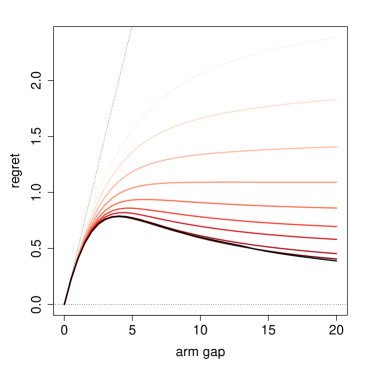
Figure 1: Regret profile for two-armed Thompson sampling, for $c=1$, 1/2, 1/4, 1/8, 1/16, 1/32, 1/64, 1/256, 1/1024, and finally $c=0$. We use $\sigma^{2}=1$ throughout. The left panel shows expected regret, while the right panel shows $\mathbb{E}\left[Q_{1}\right]$. The curves with positive values are shown in hues of red with darker-colored hues corresponding to smaller values of $c$, while $c=0$ is shown in black. The algorithm (4.8) is translation-invariant and symmetric in its treatment of the arms, so regret only depends on the scaled arm gap $\delta=\left\lvert\mu_{1}-\mu_{2}\right\rvert$.

This analysis immediately reveals an intriguing relation between the regularization parameter $c$ and regret. The Bayesian heuristic behind Thompson sampling appears to be mostly uninformative about which choices of $c$ will perform well in terms of regret; and instead, in the region and to the resolution displayed, regret appears instance-wise monotone increasing in $c$ (i.e., for each arm gap $\delta$ and each pair of regularization parameters $c_{1}<c_{2}$ displayed, we obtain lower regret with $c_{1}$). We also see that regret in fact converges as $c\rightarrow 0$, and that undersmoothed Thompson sampling appears instance-wise optimal. Thus, black our analysis based on the diffusion limit suggests that if a practitioner wants to use two-armed Thompson sampling and has prior information about the size of the gap between the two arms, then they may actually be best off ignoring this information in choosing the prior for Thompson sampling and instead using an undersmoothed specification.

	Regret (original)	Scaled regret	Reference
UCB	$3\Delta_{n}+16\log(n)/\Delta_{n}$	$+\infty$	LS20, §7.1
Thompson	${\log(n)\Delta_{n}/}{D(\mu^{n}_{1},\,\mu^{n}_{2})}$	$+\infty$	AG17
MOSS	$39\sqrt{2n}+\Delta_{n}$	$55.2$	LS20, §9.1
Impr. UCB	$\min\left\{\Delta_{n}+32\frac{\log((\Delta^{n})^{2}n)}{\Delta^{n}}+\frac{96}{\Delta^{n}},n\Delta^{n}\right\}$	$\min\left\{64\frac{\log(\Delta)}{\Delta}+\frac{96}{\Delta},\Delta\right\}$	AO10
Oracle ETC	$\min\left\{\frac{4}{\Delta^{n}}\left(1+\log\left(\frac{n(\Delta^{n})^{2}}{4}\right)^{+}\right),n\Delta^{n}\right\}$	$\min\left\{\frac{4}{\Delta}\left(1+\log(\Delta^{2}/4)^{+}\right),\Delta\right\}$	LS20, §6.1

Table 1: Comparison with existing finite-time instance-dependent regret bounds. The column of scaled regret corresponds to what the bound would become under black weak signal scaling, where $\mu_{k}^{n}=\mu_{k}/\sqrt{n}$ and $\Delta^{n}=\Delta/\sqrt{n}$, with $n\to\infty$. The algorithms under consideration are the upper confidence bound (UCB) algorithm of Lai and Robbins (1985), Thompson sampling, the Minimax Optimal Strategy in the Stochastic case (MOSS) from Audibert and Bubeck (2009), improved UCB by Auer and Ortner (2010), and an oracle explore-then-commit (ETC) baseline that takes uniformly random actions up to a deterministic time chosen using a-priori knowledge of the effect size $\left\lvert\delta\right\rvert$, and then commits to the most promising arm for the rest of time. The specific bounds are as reported in Agrawal and Goyal (2017, AG17), Auer and Ortner (2010, AO10) and Lattimore and Szepesvári (2020, LS20).

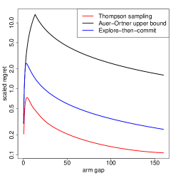
Figure 2: Comparison between the scaled regret black under the weak signal scaling for undersmoothed Thompson sampling and existing bounds in Table 1, as function of the arm gap. Here, we have a two-armed bandit with $\sigma=1$. We plot all bounds with a finite scaled regret, with the exception of MOSS, which has a constant value of 55.2 in this case.

Next, we can move beyond internal comparisons of different prior choices for Thompson sampling, and use our diffusion limit to compare large sample behavior of (undersmoothed, translation-invariant) Thompson sampling to other available baselines. In Table 1, we collect a number of state-of-the-art finite-sample bounds for two-armed bandits (we do not have access to exact diffusion-scale regret limits for these methods). We report results both in the original finite-sample form of the bound, and the (scaled) limit of the bound under the black weak signal regime from Definition 3.

A first interesting finding is that many available regret bounds are in fact vacuous in the black weak signal regime, and do not provide any meaningful control on regret. For example, while we know from our black analysis of the diffusion limit that Thompson sampling gets bounded (and in fact quite good) regret under black the weak signal scaling, the strongest available finite-sample regret bound for Thompson sampling, due to Agrawal and Goyal (2017), diverges under black the weak signal scaling. The only upper bound given in Table 1 that both remains finite under black the weak signal scaling and has meaningful instance-dependent behavior (i.e., that improves as the scaled arm gap $\delta$ gets large) is the bound of Auer and Ortner (2010) for improved UCB. We also note that the oracle explore-then-commit gets good instance-dependent behavior; however, this algorithm relies on a-priori knowledge of the arm gap size $\left\lvert\delta\right\rvert$, and so it is not a feasible baseline. Thus, any non-trivial bounds obtained via a diffusion-based analysis are likely to be stronger then many available bounds in regimes where they apply. Overall, this highlights the insight that the moderate data regime captured by the black weak signal asymptotics is in fact a challenging one, where the sample size and arm gap scale together in such a way that only the sharpest analyses yield non-trivial guarantees on performance.

Finally, in cases where the bounds from Table 1 are not vacuous black under the weak signal scaling, Figure 2 compares our limiting regret to the relevant upper bounds. Interestingly, we see that the limiting regret we obtain for Thompson sampling is much lower than any of the available upper bounds, and Thompson sampling even outperforms the oracle explore-then-commit algorithm where the duration of exploration is optimized with a-priori knowledge of the effect size and time horizon. These examples suggest that existing finite-sample instance-dependent regret upper bounds could still be improved substantially, possibly by leveraging the black weak signal asymptotics advanced in this work.

5 The (In)stability of Sensitive Sampling Functions

The diffusion limits black that arise from the weak signal scaling also allow us to conduct refined performance analysis that goes beyond mean rewards. In this section, we use the distributional characterization of the diffusion limit to unearth some interesting instability properties of a certain family of “sensitive” sampling functions, where the sampling probability of choosing the optimal arm can swing wildly between very large to the very small. This family also includes Thompson sampling as a special case. Both our numerical results and the theoretical analysis in the preceding sections point to the fact that undersmoothed Thompson sampling ($c=0$) yields far superior total regret than its smoothed counterpart. However, this performance improvement from undersmoothing, as it turns out, does not come for free. Although undersmoothed Thompson sampling identifies and focuses on the correct best action often enough to achieve low average regret, it is also liable to fail completely and double down on a bad arm.

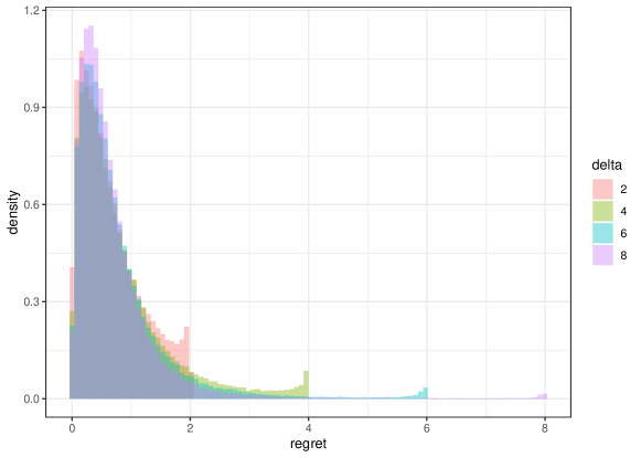
Figure 3: Distribution of the (scaled) regret for two-armed Thompson sampling in the undersmoothed regime (i.e., with $c=0$), as a function of (scaled) arm gap $\delta$. The histograms are aggregated over 100,000 realization of the limiting stochastic differential equation.

As a first lens on the instability of Thompson sampling, Figure 3 displays the distribution of regret for undersmoothed two-armed Thompson sampling for a variety of arm gaps $\delta$. Interestingly, we see that for all considered values of $\delta$, the distribution of regret is noticeably not unimodal. Rather, there is a primary mode corresponding to the bulk of realizations where Thompson sampling gets reasonably low regret, but there is also a second mode near $R\approx\delta$. Recall that, if $\mu_{1}>\mu_{2}$, then regret measures the frequency of draws on the second arm $R=\left\lvert\delta\right\rvert Q_{2,1}$, and in particular $\left\lvert R\right\rvert\leq\left\lvert\delta\right\rvert$ almost surely. Thus realizations of Thompson sampling with $R\approx\delta$ correspond to cases where the algorithm almost immediately settled on the bad arm, and never really even gave the good arm a chance.

To probe deeper into the underlying cause of this instability phenomenon, we will analyze a family of simplified, one-armed adaptive experiments. In this setting, the agent is tasked with choosing between an uncertain arm (arm 1), with unknown mean reward $\mu^{n}$ and known reward variance $(\sigma^{n})^{2}$, and a default option (arm 2), with mean reward $\mu_{0}$. Without loss of generality, we will assume that the default mean reward is equal to $0$. We are interested in the black weak signal regime where $\lim_{n\rightarrow\infty}\sqrt{n}\mu^{n}=\mu$ for some fixed $\mu\in\mathbb{R}$ while $\lim_{n\rightarrow\infty}\sigma^{n}=\sigma$ remains constant. We will refer to $\mu$ as the effect size of the experiment, which can also be thought of as the diffusion-scaled arm gap between the unknown and default arms.

Example 6 (One-Armed Thompson sampling).

As an example of a one-armed experiment, we can apply the Thompson sampling algorithm described (2.6), where the default option would have a posterior mean reward distribution that is concentrated at zero at all times. We assume that the agent takes the reward distribution of the uncertain arm $P^{n}$ to be a Gaussian distribution with (unknown) mean $\mu^{n}$ and (known) variance $\sigma^{2}$, and sets $G_{0}^{n}$ to be a Gaussian prior on $\mu^{n}$ with mean 0. Thus, writing $Q_{i}$ for the total number of samples we have drawn the uncertain arm by period $i$ and $S_{i}$ for the sum of these samples, we have

$$\begin{split}&\mu^{n}\,\big{|}\,G_{i}^{n}\sim\mathcal{N}\left(\frac{\sigma^{-2}S_{i}}{\sigma^{-2}Q_{i}+\left(\nu^{n}\right)^{-2}},\ \ \frac{1}{\sigma^{-2}Q_{i}+\left(\nu^{n}\right)^{-2}}\right),\\ &\pi_{i}=\Phi\left(\frac{\sigma^{-2}S_{i}}{\sqrt{\sigma^{-2}Q_{i}+\left(\nu^{n}\right)^{-2}}}\right),\end{split}$$ (5.1)

where $(\nu^{n})^{2}$ is the prior variance and $\Phi$ is the standard Gaussian cumulative distribution function. In particular, we will assume that $\lim_{n\rightarrow\infty}(\nu^{n})^{-2}/n=c,\ c\geq 0.$ As before, this Thompson sampling algorithm is considered smoothed if $c>0$, and undersmoothed, if $c=0$. With this choice of prior variance, we obtain a limiting sampling probability for the uncertain arm in the black weak signal regime:

$$\psi_{1}(q,s)=\Phi\left(\frac{s}{\sigma\sqrt{q+\sigma^{2}c}}\right).$$ (5.2)

We now formulate the following notion of sensitive sampling functions within the family of one-armed experiments.

Definition 5.

Consider a one-armed experiment. We say that a limiting sampling function, $\psi(q,s)$, is sensitive, if

1. for any sequence $\{(q_{n},s_{n})\}_{n\in\mathbb{N}}$ such that $\lim_{n\to\infty}s_{n}/\sqrt{q_{n}}=\infty$, we have

   $$\lim_{n\to\infty}\psi(q_{n},s_{n})=1;$$ (5.3)

2. for any sequence $\{(q_{n},s_{n})\}_{n\in\mathbb{N}}$ such that $\lim_{n\to\infty}s_{n}/\sqrt{q_{n}}=-\infty$, we have

   $$\lim_{n\to\infty}\psi(q_{n},s_{n})=0.$$ (5.4)

In words, a sampling function is sensitive if the policy would assign probability either one or zero to drawing from the uncertain distribution, in the limit as $s/\sqrt{q}$ tends to positive or negative infinity, respectively. The quantity $s/\sqrt{q}$ arises, for instance, under a Bayesian interpretation of the uncertain mean under a diffusive prior. Consider the Gaussian one-armed experiment described in Example 6. In this case, when the prior variance $(\nu^{n})^{2}$ is very large, the agent’s posterior belief on the effect size $\mu^{n}$ admits a Gaussian distribution in period $i$ with mean $S_{i}/Q_{i}$ and standard deviation $1/\sqrt{Q_{i}}$. The value $S_{i}/\sqrt{Q_{i}}$ is therefore the z-score associated with $\mu^{n}$.

The following theorem characterizes the the evolution of the sampling probabilities $\pi_{t}$ over time under any sensitive sampling function in a one-armed experiment. Qualitatively, these sampling probabilities $\pi_{t}$ can be thought of as the agent’s subjective preference about which arm is the best. In this case, we find that a sensitive sampling function will always lead the black agent to committing to the “wrong” superior arm with arbitrarily high intensity at some point during the sampling process, and that this is true no matter how large the magnitude of the actual effect size.

Theorem 10.

Fix a one-armed experiment and a continuous limiting sampling function $\psi$ that is also sensitive as per Definition 5. Consider the sampling probability $\pi_{t}=\psi(Q_{t},S_{t})$ associated with the diffusion limit under $\psi$, where $Q$ and $S$ correspond to the state of the uncertain arm. Then, fixing any effect size $\mu\in\mathbb{R}$ and confidence level $\eta\in(0,1)$, we have, for all $\epsilon\in(0,1)$,

$$\mathbb{P}\left(\sup_{t\in[0,\epsilon)}\pi_{t}\geq 1-\eta\right)=\mathbb{P}\left(\inf_{t\in[0,\epsilon)}\pi_{t}\leq\eta\right)=1.$$ (5.5)

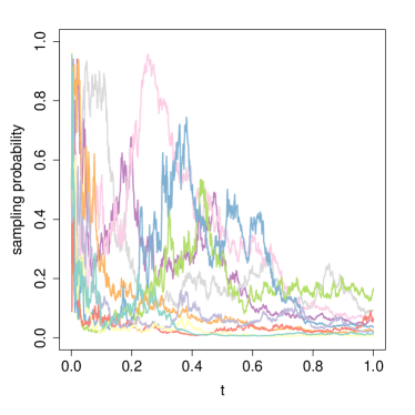
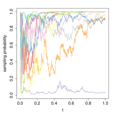
$\mu=-3$	$\mu=3$

Figure 4: Sample paths of the sampling probability $\pi_{t}$ in one-armed Thompson sampling as defined in (5.1), in the undersmoothed regime (i.e., with $c=0$).

The key idea in the proof of Theorem 10, given in Appendix A.8, is to use the time-changed form of the diffusion limit given in Theorems 3. In particular, we show that under the weak signal scaling, the quantity $S_{t}/\sqrt{Q_{t}}$ can be written via the time-change formula such that a leading determinant of its value is $W_{Q_{t}}/\sqrt{Q_{t}}$, where $W_{q}$ is a standard Brownian motion. By the law of iterated logarithm, we know that $W_{q}/\sqrt{q}$ will get arbitrarily close to $\pm\infty$ as $q\downarrow 0$, which, using the definition of a sensitive sampling function, we can use to show that $\pi_{t}$ will in turn spend time arbitrarily close to $0$ and $1$ as $t\downarrow 0$. A similar result also holds for the two-armed case, although its proof is not as immediate so we do not provide it here.

In words, Theorem 10 shows that an agent using a sensitive sampling function will almost always at some early point in time be arbitrarily convinced about $\mu$ having the wrong sign; and this holds no matter how large the effect size $\left\lvert\mu\right\rvert$ really is. One consequence of this finding is that it challenges a perspective that would take Thompson sampling literally as a principled Bayesian algorithm (since in this case we’d expect belief distributions to follow martingale updates), and instead highlights that Thompson sampling has subtle and unexpected behaviors that can only be elucidated via dedicated methods.

6 Discussion

In this paper, we introduced a black weak signal asymptotic regime under which sequentially randomized experiments converge to a diffusion limit. In particular, the limit cumulative reward is obtained by applying a random time change to a constant-drift Brownian motion, where the time change is in turn given by cumulative sampling probabilities (Theorem 3). We then applied this result to derive sharp insights about the behavior of Lipschitz-continuous sampling functions and undersmoothed two-armed Thompson sampling. Notably, we demonstrate that Lipschitz-continuous sampling always leads to non-vanishing, and thus sub-optimal, regret when the arm gaps are large. In contrast, we show that using an asymptotically uninformative prior with two-armed Thompson sampling leads to desirable regrets across all arm gaps in the black weak signal regime, and especially when the arm gap is large, where we show the regret is nearly instance-optimal. This latter result is one of the first recent attempts at formally justifying the folklore wisdom of using diffusive priors in Thompson sampling (e.g., Liu et al., 2022), where, for instance, it is recommended to set the prior variance to a fixed large constant (Agrawal and Goyal, 2017).

A first class of natural follow-up questions is in seeing whether diffusion limits hold for broader classes of sequential experiments. The current diffusion analysis leaves out those experiments that have a discontinuous sampling function, which include, for instance, UCB-type experiments. A key technical challenge in analyzing discontinuous sampling functions is that the number of arm pulls under them can be highly erratic, which makes showing the convergence to a diffusion limit more challenging. After we posted a version of this paper online, the recent work by Kalvit and Zeevi (2021) made progress towards this question by showing a diffusion limit for a two-armed UCB algorithm. Their analysis relies on a refined regularity property of UCB where they show that both arms will be pulled approximately an equal number of times as the number of samples grows. It remains unclear whether such analysis can be generalized beyond UCB with two arms, or to other discontinuous sampling functions. Furthermore, it would be interesting to see whether our results can be extended to the case of contextual bandits, or to bandit problems with continuous action spaces that arise, e.g., with pricing. Finally, another practical question is whether the approach used here can be used to build confidence intervals using data from sequential experiments, thus adding to the line of work pursued by Hadad et al. (2021), Howard et al. (2021), Zhang et al. (2020), and others.

Another set of questions could aim to characterize the rate of convergence to the diffusion limit, which we do not consider in the current paper. Such results can be useful in quantifying the quality of black weak signal asymptotics for finite-sample experiments. It would be interesting, for instance, to understand how the quality of approximation depends on the smoothness of the sampling function.

Further along, a potentially interesting avenue for investigation is whether the diffusion limit derived here is useful in understanding human—as opposed to algorithmic—learning. Throughout this paper, we have considered Thompson sampling and related algorithms as a class of sequential experiments designed by an investigator, and have discussed how different design choices (e.g., around smoothing) affect the performance of the learning algorithms. However, following Erev and Roth (1998) and Xu and Yun (2020), we could alternatively use sequentially randomized Markov experiments as models for how humans (or human communities) learn over time, and use our results to make qualitative predictions about their behavior. For example, it may be of interest to examine Thompson sampling as a model for how a scientific community collects and assimilates knowledge about different medical treatments. Qualitatively, this would correspond to a hypothesis that the number of scientists investigating any specific treatment should be proportional to the consensus beliefs that the treatment is best given the available evidence at the time (i.e., that scientists at any given time prioritize investigating the treatments that appear most promising). In this case, our Theorem 10 would provide conditions under which we predict consensus beliefs to first temporarily concentrate around sub-optimal treatments before eventually reaching the truth. More broadly, the many unintuitive phenomena arising from our diffusion limits could yield a number of valuable insights on how we collect and process information.

Supplemental Material for
Weak Signal Asymptotics for Sequentially Randomized Experiments

Appendix A Proofs of Main Results

Terminology: We will use the term “almost all sample paths” throughout the proofs to refer to sample paths of the Brownian motion that belong to a set of probability measure one. We will also use the following asymptotic notation: $f(x)\ll g(x)$ indicates that $f(x)/g(x)\to 0$, similarly for $f(x)\gg g(x)$.

A.1 Proof of Theorem 1

Proof. The proof is based on the martingale framework of Stroock and Varadhan [2007]. Let us first introduce some notation to streamline the presentation of the proof. Define $Z_{t}=(\widebar{Q}_{t},\widebar{S}_{t})$. Denote by $\mathcal{I}_{S}$ and $\mathcal{I}_{Q}$ the indices in $Z_{t}$ corresponding to the coordinates of $S$ and $Q$, respectively. Both sets are understood to be an ordered set of $K$ elements, where the subscript is for distinguishing whether the ordering is applied to $S$ versus $Q$. For $z\in\mathbb{R}_{+}^{K}\times\mathbb{R}^{K}$, define the functions $(b_{k})_{k\in\mathcal{I}_{Q}\cup\mathcal{I}_{S}}$,

$$b_{k}(z)= \begin{cases}\psi_{k}(z),&k\in\mathcal{I}_{Q},\\ \psi_{k}(z)\mu_{k},&k\in\mathcal{I}_{S}.\end{cases}$$ (A.1)

For $1\leq k,l\leq K$, define

$$\eta_{k,l}(z)= \begin{cases}\sqrt{\psi_{k}(z)}\sigma_{k},&\text{if $k=l\in\mathcal{I}_{S}$,}\\ 0,&\text{otherwise.}\end{cases}$$ (A.2)

Then, the Itô diffusion SDE in (3.1) can be written more compactly as

$$dZ_{t}=b(Z_{t})dt+\eta(Z_{t})dB_{t},\quad t\in[0,1],$$ (A.3)

with $Z_{0}=0$.

Next, we briefly review the relevant results of the Stroock and Varadhan program. Fix $d\in\mathbb{N}$. Let $(Z^{n}_{i})_{i\in\mathbb{N}}$ be a sequence of time-homogeneous Markov chains taking values in $\mathbb{R}^{d}$, indexed by $n\in\mathbb{N}$. Denote by $\Pi^{n}$ the transition kernel of $Z^{n}$:

$$\Pi^{n}(z,A)=\mathbb{P}\left(Z^{n}_{i+1}\in A\,\big{|}\,Z^{n}_{i}=z\right),\quad z\in\mathbb{R}^{d},A\subseteq\mathbb{R}^{d}.$$ (A.4)

Let $\widebar{Z}^{n}_{t}$ be the piece-wise linear interpolation of $Z^{n}_{nt}$:

$$\widebar{Z}^{n}_{t}=(1-tn+\lfloor tn\rfloor)Z^{n}_{\lfloor tn\rfloor}+(tn-\lfloor tn\rfloor)Z^{n}_{\lfloor tn\rfloor+1},\quad t\in[0,1].$$ (A.5)

Define $K^{n}(z,A)$ to be the scaled transition kernel:

$$K^{n}(z,A)=n\Pi^{n}(z,A).$$ (A.6)

Finally, define the functions

$$a^{n}_{k,l}(z)= \int_{x:|z-x|\leq 1}(x_{k}-z_{k})(x_{l}-z_{l})K^{n}(z,dx),$$

$$b^{n}_{k}(z)= \int_{x:|z-x|\leq 1}(x_{k}-z_{k})K^{n}(z,dx),$$

$$\Delta^{n}_{\epsilon}(z)= K^{n}(z,\{x:|x-z|>\epsilon\}).$$

We will use the following result. A proof of the theorem can be found in Stroock and Varadhan [2007, Chapter 11] or Durrett [1996, Chapter 8]. For conditions that ensure the uniqueness and existence of the Itô diffusion (A.10), see Karatzas and Shreve [2005, Chapter 5, Theorem 2.9].

Theorem 11.

Fix $d$. Let $\{a_{k,l}\}_{1\leq k,l\leq d}$ and $\{b_{k}\}_{1\leq k\leq d}$ be bounded Lipschitz-continuous functions from $\mathbb{R}^{d}$ to $\mathbb{R}$. Suppose that for all $k,l\in\{1,\ldots,d\}$ and $\epsilon,R>0$

$$\lim_{n\to\infty}\sup_{z:|z|<R}|a^{n}_{k,l}(z)-a_{k,l}(z)|=0,$$ (A.7)

$$\lim_{n\to\infty}\sup_{z:|z|<R}|b^{n}_{k}(z)-b_{k}(z)|=0,$$ (A.8)

$$\lim_{n\to\infty}\sup_{z:|z|<R}\Delta^{n}_{\epsilon}(z)=0.$$ (A.9)

If $\widebar{Z}^{n}_{0}\to z_{0}$ as $n\to\infty$, then $(\widebar{Z}^{n}_{t})_{t\in[0,1]}$ converges weakly in $\mathcal{C}$ to the unique solution to the stochastic differential equation

$$dZ_{t}=b(Z_{t})dt+\eta(Z_{t})dB_{t},$$ (A.10)

where $Z_{0}=z_{0}$ and $\{\eta_{k,l}\}_{1\leq k,l\leq d}$ are dispersion functions such that $a(z)=\eta(z)\eta^{\intercal}(z)$.

We are now ready to prove Theorem 1. We will use the compact representation of the SDE given in (A.3), with $\widebar{Z}^{n}=(\widebar{Q}^{n},\widebar{S}^{n})$, $Z_{t}=(Q_{t},S_{t})$ and $b$ and $\eta$ defined as in (A.1) and (A.2), respectively. To prove the convergence of $\widebar{Z}^{n}$ to the suitable diffusion limit, we will evoke Theorem 11 (here $d\leftrightarrow 2K$). It suffices to verify the convergence of the corresponding generators in (A.7) through (A.8). To start, the following technical lemma [Durrett, 1996, Section 8.8] will simplify the task of proving convergence by removing the need of truncation in the integral; the proof is given in Section C.1. Define

$$m^{n}_{p}(z)=\int|x-z|^{p}K^{n}(z,dx),\ \ \ \ \ \tilde{a}^{n}_{k,l}(z)= \int(x_{k}-z_{k})(x_{l}-z_{l})K^{n}(z,dx),$$

$$\tilde{b}^{n}_{k}(z)=\int(x_{k}-z_{k})K^{n}(z,dx).$$

Lemma 12.

Fix $p\geq 2$ and suppose that for all $R<\infty$,

$$\lim_{n\to\infty}\sup_{z:|z|<R}m^{n}_{p}(z)=0.$$ (A.11)

$$\lim_{n\to\infty}\sup_{z:|z|<R}|\tilde{a}^{n}_{k,l}(z)-a_{k,l}(z)|=0,$$ (A.12)

$$\lim_{n\to\infty}\sup_{z:|z|<R}|\tilde{b}^{n}_{k}(z)-b_{k}(z)|=0,$$ (A.13)

Then, the convergence in (A.7) through (A.9) holds.

In what follows, we will use $z=(q,s)$ to denote a specific state of the Markov chain $\widebar{Z}^{n}$. The transition kernel of the pre-limit chain $\widebar{Z}^{n}$ can be written as

$$\Pi^{n}((q,s),(q+{e_{k}}/{n},s+e_{k}ds/\sqrt{n}))=\bar{\psi}^{n}_{k}(q,s)P^{n}_{k}(ds),\quad k=1,\ldots,K,$$ (A.14)

and zero elsewhere, where $e_{k}\in\{0,1\}^{K}$ is the unit vector where the $k$th entry is equal to $1$ and all other entries are $0$, and $\{P^{n}_{k}\}_{k=1,\ldots,K}$ are the reward probability measures. Define $K^{n}(z,A)=n\Pi^{n}(z,A)$.

We next define the limiting functions $a$ and $b$. The function $b$ is defined as in (A.1):

$$b_{k}(z)= \begin{cases}\psi_{k}(z),&k\in\mathcal{I}_{Q},\\ \psi_{k}(z)\mu_{k},&k\in\mathcal{I}_{S},\end{cases}$$ (A.15)

and we let

$$a_{ij}(z)=(\eta\eta^{\intercal})_{k,l}(z)$$ (A.16)

where $\eta$ is defined in (A.2). That is,

$$a_{k,l}(z)= \begin{cases}{\psi_{k}(z)}\sigma_{k}^{2},&\text{if $k=l\in\mathcal{I}_{S}$,}\\ 0,&\text{otherwise.}\end{cases}$$ (A.17)

Fix $R>0$. We show that the corresponding $a^{n}$ and $b^{n}$ converge to the functions $a$ and $b$ defined above, uniformly over the compact set $\{z:|z|\leq R\}$. In light of Lemma 12, it suffices to verify the convergence in (A.11) through (A.13) for $p=4$. Starting with (A.11), we have that

$$m^{n}_{4}(z)= \int|z^{\prime}-z|^{4}n\Pi^{n}(z,dz^{\prime})$$

$$= \sum_{k=1}^{K}n\bar{\psi}^{n}_{k}(z)\int_{w\in\mathbb{R}}\left(\frac{1}{n^{2}}+\frac{w^{2}}{n}\right)^{2}P^{n}_{k}(dw)$$

$$\leq \sum_{k=1}^{K}n\bar{\psi}^{n}_{k}(z)\left(\frac{2}{n^{4}}+\frac{1}{n^{2}}\int_{w\in\mathbb{R}}w^{4}P^{n}_{k}(dw)\right)$$

$$= \frac{2}{n}+\frac{1}{n}\mathbb{E}_{Z\sim P^{n}_{k}}\left[Z^{4}\right]$$

$$\stackrel{{\scriptstyle n\to\infty}}{{\longrightarrow}} 0,$$ (A.18)

as $n\to 0$, uniformly over all $z$, where the last step follows from the assumption that the reward distributions admit bounded fourth moments. This shows (A.11).

For the drift term $b$, we consider the following two cases; together, they prove (A.13).

Case 1, $k\in\mathcal{I}_{Q}$. For all $k\in\mathcal{I}_{Q}$, and $n\in\mathbb{N}$,

$$\tilde{b}^{n}_{k}(z)= \int(q^{\prime}_{k}-q_{k})K^{n}(z,dz^{\prime})$$

$$= \frac{1}{n}(n\bar{\psi}^{n}_{k}(z))$$

$$\stackrel{{\scriptstyle n\to\infty}}{{\longrightarrow}} \psi_{k}(z).$$ (A.19)

Case 2, $k\in\mathcal{I}_{S}$. For all $k\in\mathcal{I}_{S}$,

$$\tilde{b}^{n}_{k}(z):= \int(s^{\prime}_{k}-s_{k})K^{n}(z,dz^{\prime})$$

$$= \bar{\psi}^{n}_{k}(z)n\int\frac{w}{\sqrt{n}}P^{n}_{k}(dw)$$

$$= \bar{\psi}^{n}_{k}(z)\mu_{k}$$

$$\stackrel{{\scriptstyle n\to\infty}}{{\longrightarrow}} b_{k}(z).$$ (A.20)

For the variance term $a$, we consider the following three cases:

Case 1, $k,l\in\mathcal{I}_{Q}$. Note that under the multi-armed bandit model, only one arm can be chosen at each time step. This means that only one coordinate of $\widebar{Q}^{n}$ can be updated at time, immediately implying that for all $n$ and $k,l\in\mathcal{I}_{Q}$, $k\neq l$,

$$\tilde{a}^{n}_{k,l}(z)=\int(q^{\prime}_{k}-q_{k})(q^{\prime}_{l}-q_{l})K^{n}(z,dz^{\prime})=0.$$ (A.21)

For the case $k=l$, we note that for all $k\in\mathcal{I}_{Q}$, and all sufficiently large $n$

$$\tilde{a}^{n}_{k,k}(z)=\frac{1}{n^{2}}n\bar{\psi}^{n}_{k}(z)\stackrel{{\scriptstyle n\to\infty}}{{\longrightarrow}}0.$$ (A.22)

Case 2: $k\in\mathcal{I}_{Q},l\in\mathcal{I}_{S}$, or $k\in\mathcal{I}_{S}$ and $l\in\mathcal{I}_{Q}$.

$$\tilde{a}^{n}_{k,l}(z)= \int(q^{\prime}_{k}-q_{k})(q^{\prime}_{l}-q_{l})K^{n}(z,dz^{\prime})$$

$$= \frac{\bar{\psi}^{n}_{k}(z)}{n}\int w(nP^{n}_{k}(\sqrt{n}dw))$$

$$= \bar{\psi}^{n}_{k}(z)\mathbb{E}_{Z\sim P^{n}_{k}}\left[Z\right]$$

$$= \bar{\psi}^{n}_{k}(z)\mu_{k}/\sqrt{n}$$

$$\stackrel{{\scriptstyle n\to\infty}}{{\longrightarrow}} 0.$$ (A.23)

Case 3: $k,l\in\mathcal{I}_{S}$. This case divides into two further sub-cases. Suppose that $k\neq l$. Similar to the logic in Case 1, because only one coordinate of $\widebar{Q}^{n}$ can be updated at a given time step, we have

$$\tilde{a}^{n}_{k,l}(z)=0,\quad k\neq l.$$ (A.24)

Suppose now that $k=l$. We have

$$\tilde{a}^{n}_{k,l}(z)= \int(q^{\prime}_{k}-q_{k})^{2}K^{n}(z,dz^{\prime})$$

$$= {\bar{\psi}^{n}_{k}(z)}\int w^{2}(nP^{n}_{k}(\sqrt{n}dw))$$

$$= \bar{\psi}^{n}_{k}(z)\mathbb{E}_{Z\sim P^{n}_{k}}\left[Z^{2}\right]$$

$$\stackrel{{\scriptstyle n\to\infty}}{{\longrightarrow}} \psi_{k}(z)\sigma_{k}^{2}$$

$$= a_{k,l}(z).$$ (A.25)

We note that by assuming that the limiting sampling function $\psi$ is Lipschitz-continuous, the convergence of $\tilde{b}^{n}$, $\tilde{a}^{n}$ and $m^{n}_{p}$ to their respective limits holds uniformly over compact sets. We have thus verified the conditions in Lemma 12, further implying (A.7) through (A.8). Note that because $\psi_{k}$ is bounded and Lipschitz-continuous, so are $a$ and $b$. This proves the convergence of $\widebar{Z}^{n}$ to the diffusion limit in $\mathcal{C}$.

Finally, to prove the convergence of $\mathbb{E}\left[f(\widebar{Z}^{n}_{1})\right]$ to $\mathbb{E}\left[f(Z_{t})\right]$, note that the weak convergence of $\widebar{Z}^{n}$ in $\mathcal{C}$ implies that the marginal distribution, $\widebar{Z}^{n}_{t}$ converges weakly to $Z_{t}$, as $n\to\infty$. The result then follows immediately from the continuous mapping theorem and the bounded convergence theorem. This completes the proof of Theorem 1. ∎

A.2 Proof of Theorem 3

Proof. It suffices to show that (3.7) holds. We will begin with a slightly different, but equivalent, characterization of the pre-limit bandit dynamics. Consider the $n$th problem instance. Denote by $\tilde{Y}_{k,j}$ the reward obtained from the $j$th pull of arm $k$. Then, we have that for a fixed $k$, $\tilde{Y}_{k,\cdot}$ is an i.i.d. sequence, independent from all other aspects of the system, and

$$S_{k,i}=\sum_{j=1}^{Q_{k,i}}\tilde{Y}_{k,j}.$$ (A.26)

We can further write

$$\tilde{Y}_{k,j}=\mu_{k}/\sqrt{n}+U_{k,j},$$ (A.27)

where $U_{k,j}$ is a zero-mean random variable with variance $\sigma_{k}^{2}$. Define the scaled process:

$$U^{n}_{k,i}=\frac{1}{\sqrt{n}}\sum_{j=1}^{i}U_{k,j}.$$ (A.28)

We thus arrive at the following expression for the diffusion-scaled cumulative reward:

$$\widebar{S}^{n}_{k,t}=\widebar{Q}^{n}_{k,t}\mu_{k}+U^{n}_{k,n\widebar{Q}^{n}_{k,t}},\quad i=1,\ldots,n.$$ (A.29)

Denote by $\bar{U}^{n}_{k,t}$ to be the linear interpolation of $U^{n}_{k,\lfloor nt\rfloor}$ for $t\in[0,1]$. By Donsker’s theorem, there exists a $K$-dimensional standard Brownian motion $W$ such that $\bar{U}^{n}$ converges to $\{\sigma_{k}W_{k,\cdot}\}_{k=1,\ldots,K}$ weakly in $\mathcal{C}$. Evoking Theorem 1 and the Skorohod’s representation theorem [Billingsley, 1999, Theorem 6.7], we may construct a probability space on which the following convergences in $\mathcal{C}$ occur almost surely:

$$\widebar{S}^{n}_{k,t}\to S_{k,t},\,\widebar{Q}^{n}_{k,t}\to Q_{k,t},\,\bar{U}^{n}_{t}{k,t}\to\sigma_{k}W_{k,t},$$ (A.30)

as $n\to\infty$, where $S$ and $Q$ are diffusion processes satisfying the SDEs in Theorem 1.

We now combine (A.29) and (A.30), along with the fact that $W$ is uniformly continuous in the compact interval $[0,1]$, to conclude that almost surely

$$U^{n}_{k,n\widebar{Q}^{n}_{k,i}}\to\sigma_{k}W_{k,Q_{k,t}},$$ (A.31)

in $\mathcal{C}$. This further implies that $S$ also satisfies

$$S_{k,t}=Q_{k,t}\mu_{k}+\sigma_{k}W_{k,Q_{k,t}},$$ (A.32)

proving our claim.

∎

A.3 Proof of Lemma 4

Proof. For the first claim, we note that the $Q^{j}$’s are $1$-Lipschitz and therefore uniformly equicontinuous over $[0,1]$. It follows from the Arzela-Ascoli theorem that $\{Q^{j}\}$ admits a convergent subsequence $Q^{j_{m}}$. The convergence of $S^{j_{m}}$ follows directly from its characterization in (3.7) and so does the fact that $S$ satisfies (3.7). To show that $Q$ is a solution to the ODEs, let $\{Q^{j_{m}}\}_{m\in\mathbb{N}}$ be the subsequence that converges uniformly to $Q$. Because the sample path of the Brownian motion $W$ is uniformly bounded over $t\in[0,1]$ almost surely, it follows from (3.6) that the derivative $(Q^{j_{m}})^{\prime}$ converges uniformly over $(0,1)$. Combining this fact with the uniform convergence of $Q^{j_{m}}$, it follows from the fundamental theorem of calculus that $Q$ is differentiable over $(0,1)$, and $(Q^{j_{m}})^{\prime}$ converges uniformly to $Q^{\prime}$. This proves the claim. ∎

A.4 black Proof of Theorem 5

black Proof. By Theorem 3, we have that for every $j$, $(\bar{Q}^{n,j},\bar{S}^{n,j})$ converges to a unique solution to the ODEs in Theorem 3 with sampling function $\psi^{j}$, $(Q^{j},S^{j})$, as $n\to\infty$. By Lemma 4, there exists a limit function $(Q,S)$ for the sequence $\{(Q_{j},S_{j})\}_{j\in\mathbb{N}}$ and furthermore that $(Q,S)$ is a solution to the ODEs in Theorem 3 with sampling function $\psi$. The above two factors combined imply that there exists a sequence $\{j_{n}\}$, with $\lim_{n\to\infty}j_{n}=\infty$, such that $(\bar{Q}^{n,j_{n}},\bar{S}^{n,j_{n}})$ converges to $(Q,S)$ as $n\to\infty$. This proves the claim. ∎

A.5 Proof of Theorem 7

Proof. Denote by $R_{t}$ the cumulative regret up to time $t$ under the weak signal scaling. We have that for all $t\in(0,1)$:

$$R=R_{1}\geq R_{t}\geq(t-Q_{1,t})\delta.$$ (A.33)

Next, we will bound the term $(t-Q_{1,t})$ by analyzing its evolution over a small time interval near $t=0$. Define $t_{\delta}=c/\delta$, where $c$ is a constant whose value will be chosen subsequently. Recall that $Z_{t}:=(Q_{t},S_{t})$. By the Lipschitz continuity of $\psi$, we have that for all $t<t_{\delta}$, and all sufficiently large $\delta$, the following holds almost surely:

$$\psi_{1}(Z_{t})\leq \psi_{1}(0,0)+L\|Z_{t}\|$$

$$\leq \tilde{p}+L(\|Q_{t}\|+\|S_{t}\|)$$

$$\stackrel{{\scriptstyle(a)}}{{\leq}} \tilde{p}+L(Kt_{\delta}+\|S_{t}\|)$$

$$\stackrel{{\scriptstyle(b)}}{{\leq}} \tilde{p}+LK(t_{\delta}+(\tilde{m}_{1}+\delta)t_{\delta}+{t_{\delta}}^{2/3})$$

$$\leq \tilde{p}+2LK\delta t_{\delta}$$

$$= \tilde{p}+2LKc,$$ (A.34)

where step $(a)$ follows from each coordinate of $Q_{t}$ being 1-Lipschitz by construction. Step $(b)$ follows from the characterization in Theorem 3 that $S_{k,t}=Q_{k,t}\mu_{k}+\sigma_{k}W_{k,Q_{k,t}},$ where, evoking the law of iterated logarithm (Lemma 20), we conclude that, for all sufficiently large $\delta$:

$$\sigma_{k}W_{k,Q_{k,t}}\leq\sup_{0\leq u\leq Q_{k,t_{\delta}}}\sigma_{k}W_{k,u}\leq\sup_{0\leq u\leq t_{\delta}}\sigma_{k}W_{k,u}\leq{t_{\delta}}^{2/3}.$$ (A.35)

Set $c=\frac{1-\tilde{p}}{4LK}$. The above inequality implies that

$$1-\psi_{1}(Z_{t})\geq\frac{1-\tilde{p}}{2},\quad\forall t\in(0,t_{\delta}).$$ (A.36)

Combining this with (A.33), we have that for all large $\delta$:

$$R\geq(t-Q_{1,t})\delta\geq\delta\int_{0}^{t_{\delta}}1-\psi_{1}(Z_{t})ds=\delta\frac{(1-\tilde{p})/4LK}{\delta}\cdot\frac{1-\tilde{p}}{2}=\frac{(1-\tilde{p})^{2}}{8KL}.$$ (A.37)

This proves our claim. ∎

A.6 Proof of Corollary 8

Proof. For simplicity of notation, we will let $\sigma_{k}=1$ for all $k$, while the proof can be extended easily to the case where $\sigma_{k}>0$ for all $k$. For $(q,s)\in[0,1]^{K}\times\mathbb{R}^{K}$, define

$$\bar{\mu}_{k}(q,s)=\frac{s_{k}}{q_{k}+c},\quad\bar{\sigma}_{k}(q,s)=\sqrt{\frac{1}{q_{k}+c}},\quad k=1,\ldots,K.$$ (A.38)

Then, the limiting sampling function associated with Gaussian Thompson sampling, given in (2.15), can be written as:

$$\psi_{k}(q,s)=\Pi^{\sup}(q,\,s;\,\sigma^{2},\,c)=\mathbb{P}\left(N(\bar{\mu}_{k}(q,s),\bar{\sigma}_{k}(q,s)^{2})>\max_{l\neq k}N(\bar{\mu}_{l}(q,s),\bar{\sigma}_{l}(q,s)^{2})\right),$$ (A.39)

where $N(\mu,\sigma^{2})$ represents a Gaussian random variable with mean $\mu$ and variance $\sigma^{2}$, independent from the rest of the system.

Next, we show that, for all $c>0$, the sampling function in (A.39) is Lipschitz-continuous. Denote by $f^{(q,s)}$ the density of the Gaussian distribution $\mathcal{N}(\bar{\mu}(q,s),I\bar{\sigma}(q,s)^{2})$, and by $f^{(q,s)}_{k}$ the density of its $k$th marginal. Then,

$$\psi_{k}(q,s)= \int_{\mathbb{R}^{K}}f^{(q,s)}(x)\mathbb{I}(\max_{l\neq k}x_{l}<x_{k})dx$$

$$= \int_{\mathbb{R}^{K}}\left(\prod_{l=1,\ldots,K}f^{(q,s)}_{l}(x_{l})\right)\mathbb{I}(\max_{l\neq k}x_{l}<x_{k})dx.$$ (A.40)

Because $c>0$, we have that $\bar{\sigma}_{k}(q,s)$ is uniformly bounded from below by $\sqrt{1/c}$ for all $q\in[0,1]$. This implies $\bar{\mu}$ is Lipschitz, and that there exists constant $D>0$, such that

$$\left\lvert\frac{\partial}{\partial q_{l}}f^{(q,s)}_{l}(x_{l})\right\rvert\leq D,\ \ \left\lvert\frac{\partial}{\partial s_{l}}f^{(q,s)}_{l}(x_{l})\right\rvert\leq D,\quad\mbox{$\forall l=1,\ldots,K$, $x,s\in\mathbb{R}^{K}$, $q\in[0,1]^{K}$.}$$ (A.41)

Note that by the product form of $f^{(q,s)}$ and the fact that $f_{l}$ is solely determined by $(q_{l},s_{l})$, we have that

$$\frac{\partial}{\partial q_{l}}f^{(q,s)}(x)=\frac{\partial}{\partial q_{l}}\prod_{l=1,\ldots,K}f^{(q,s)}_{l}(x_{l})\leq D{\prod_{l^{\prime}\neq l}f^{(q,s)}_{l^{\prime}}(x_{l^{\prime}})}\leq\frac{D}{(2\pi/c)^{(K-1)/2}},$$ (A.42)

where step $(a)$ follows from (A.41) and $(b)$ from the fact that $\bar{\sigma}_{k}(q,s)\geq 1/\sqrt{c}$ for all $k$ and hence $f^{(q,s)}_{l^{\prime}}(x_{l^{\prime}})\leq\frac{1}{\sqrt{2\pi/c}}$. The same bound holds for $\frac{\partial}{\partial s_{l}}f^{(q,s)}(x)$ via an identical argument. Combining the above inequality with (A.40) and applying the Leibniz integral rule, we conclude that the magnitude of every coordinate of the gradient $\nabla\psi_{k}(q,s)$ is bounded from above by $\frac{D}{(2\pi/c)^{(K-1)/2}}$. This proves that $\psi(\cdot,\cdot)$ is Lipschitz-continuous. The fact that $\liminf_{\delta\to\infty}R>0$ thus follows immediately from Theorem 7.

∎

A.7 Proof of Theorem 9

We will prove Theorem 9 by showing the following stronger version, which includes a similar super diffusive regret bound for undersmoothed one-armed Thompson sampling introduced in (5.1), where only one of the two arms is uncertain. We do so because the analysis for the one-armed version of the algorithm is simpler, and will provide the crucial ingredients for understanding undersmoothed two-armed Thompson sampling.

Theorem 13.

Consider the diffusion limit associated with one- and two-armed undersmoothed Thompson sampling, with $c=0$. Then, the following holds almost surely for the diffusion regret (3.4) in the super diffusive regime.

1. For one-armed Thompson sampling,

   $$R\prec 1/|\mu|,\quad\mbox{as $|\mu|\to\infty$},$$ (A.43)

   where $\mu\in\mathbb{R}$ is the mean of the unknown arm.

2. For two-armed undersmoothed Thompson sampling,

   $$R\prec 1/\delta,\quad\mbox{as $\delta\to\infty$},$$ (A.44)

   where $\delta=\mu_{1}-\mu_{2}$ is the arm gap.

We divide the proof of the above theorem into two sections, for the one- and two-armed Thompson sampling, respectively. We begin by presenting the equivalent ODE characterization of the diffusion limit for one- and two-armed Thompson sampling using the random-time change in Theorem 3. These ODEs will be used repeatedly in our proof. Fix $c\geq 0$.

For one-armed Thompson sampling (5.1), it is not difficult to verify that the sample paths of $S^{n}$ and $Q^{n}$ associated with the uncertain arm converge weakly to the SDE:

$$dQ_{t}=\pi_{t}dt,\ \ \ \ \ \ dS_{t}=\mu\pi_{t}dt+\sqrt{\pi_{t}}dB_{t},\ \ \ \ \ \ \pi_{t}=\Phi\left(\frac{S_{t}}{\sigma\sqrt{Q_{t}+\sigma^{2}c}}\right).$$ (A.45)

which can be expressed in the ODE form as follows:

$$dQ_{t}= \Phi\left(\frac{Q_{t}\mu+W_{Q_{t}}}{\sigma\sqrt{Q_{t}+\sigma^{2}c}}\right)\,dt,\ \ \ S_{t}=\mu Q_{t}+\sigma W_{Q_{t}},$$ (A.46)

with $Q_{0}=S_{0}=0$ and $W$ is a standard one-dimensional Brownian motion. Likewise, for two-armed Thompson sampling, the following is the ODE corresponding to the SDE in (4.9):

$$\begin{split}d{Q_{1,t}}=&\Phi\left(\frac{\sigma^{-2}\left(Q_{1,t}Q_{2,t}\delta+Q_{2,t}W_{1,Q_{1,t}}-Q_{1,t}W_{2,Q_{2,t}}\right)}{\sqrt{\sigma^{-2}tQ_{1,t}Q_{2,t}+t^{2}c}}\right)dt,\\ d{Q_{2,t}}=&\Phi\left(\frac{-\sigma^{-2}\left(Q_{1,t}Q_{2,t}\delta-Q_{2,t}W_{2,Q_{1,t}}+Q_{1,t}W_{1,Q_{2,t}}\right)}{\sqrt{\sigma^{-2}tQ_{1,t}Q_{2,t}+t^{2}c}}\right)dt,\\ S_{k,t}=&\mu_{k}Q_{k,t}+\sigma_{k}W_{k,Q_{k,t}},\quad k=1,2,\end{split}$$ (A.47)

with $Q_{\cdot,0}=S_{\cdot,0}=0$, where $\delta=\mu_{1}-\mu_{2}$ and $W$ is a standard two-dimensional Brownian motion. For our subsequent analysis, we will take $\sigma=1$.

A.7.1 One-Armed Setting

Define the limit cumulative regret $R_{t}$ as:

$$R_{t}=(\mu)_{+}t-\mu Q_{t},\quad t\in[0,1],$$ (A.48)

where $Q_{t}$ is the diffusion limit associated with $Q^{n}_{i}$. Note that $R_{1}$ corresponds to the scaled cumulative regret $R$ in (3.4).

We will be working with the random-time-change version of the diffusion, as per (A.46). Define the following stopping time:

$$\tau(q)=\inf\{t:Q_{t}\geq q\},$$ (A.49)

with $\tau(q):=1$ if $Q_{1}\leq q$. As mentioned earlier, the sample paths exhibit different dynamics depending on whether $\mu$ tends to the positive or negative infinity; as such, our proof will also treat these two cases separately.

Case 1: $\mu\to-\infty$. Fix $\alpha\in(1,2)$. Recall the stopping time from (A.49) with threshold $q$. We will be particularly interested in the case where

$$q=|\mu|^{-\alpha}.$$

Decompose $R_{1}$ into two components:

$$R_{1}=R_{\tau(|\mu|^{-\alpha})}+(R_{1}-R_{\tau(|\mu|^{-\alpha})}).$$ (A.50)

We next bound the two terms on the right-hand side of the equation above separately. Since $Q_{t}$ is non-decreasing, we have

$$R_{\tau(|\mu|^{-\alpha})}=|\mu|\cdot Q_{\tau(|\mu|^{-\alpha})}=|\mu|^{-(\alpha-1)}.$$ (A.51)

For the second term, the intuition is that by the time $Q_{t}$ reaches $|\mu|^{-\alpha}$, the drift in $Q_{t}$ will have already become overwhelmingly small for the rest of the time horizon. To make this rigorous, note the following facts:

1. By the law of iterated logarithm of Brownian motion, along almost all sample paths of $W$, there exists constant $C$ such that

   $$\limsup_{\mu\to-\infty}\sup_{x\in[\tau(|\mu|^{-\alpha}),1]}\left|\frac{W_{x}}{\sqrt{x}}\right|\leq C\sqrt{\log\log(|\mu|^{\alpha})}.$$ (A.52)

2. $\mu\sqrt{Q_{\tau(|\mu|^{-\alpha})}}=-|\mu|^{1-\alpha/2}$, and therefore $\frac{\mu\sqrt{Q_{\tau(|\mu|^{-\alpha})}}}{2}\ll-\sqrt{\log\log(|\mu|^{\alpha})}$ as $\mu\to-\infty$.

Combining these facts along with the normal cdf tail bounds from Lemma 19 in Section B, we have that along almost all sample paths of $W$, there exists constant $b>0$, such that for all sufficiently small $\mu$,

$$R_{1}-R_{\tau(|\mu|^{-\alpha})}= |\mu|\int_{\tau(|\mu|^{-\alpha})}^{1}\Pi(0,Q_{t})dt$$

$$\leq |\mu|\left(\sup_{t\in[\tau(|\mu|^{-\alpha}),1]}\Phi\left(\frac{\mu\sqrt{Q_{t}}}{\sigma}+\frac{W_{Q_{t}}}{\sigma\sqrt{Q_{t}}}\right)\right)$$

$$\stackrel{{\scriptstyle(a)}}{{\leq}} |\mu|\Phi\left(-|\mu|^{1-\alpha/2}+C\sqrt{\log\log(|\mu|^{\alpha})}\right)$$

$$\leq |\mu|\exp(-|\mu|^{b}),$$ (A.53)

where $(a)$ follows from the aforementioned facts. Putting together (A.51) and (A.53) shows that

$$R_{1}\leq\mu^{-(\alpha-1)}+|\mu|\exp(-|\mu|^{b})\stackrel{{\scriptstyle\mu\to\infty}}{{\prec}}\mu^{-(\alpha-1)},\quad a.s.$$ (A.54)

This proves the claim by noting that the above holds for all $\alpha\in(1,2)$.

Case 2: $\mu\to\infty$. In this case, we would like to argue that $Q_{t}$ will increase rapidly as $\mu$ grows. Let $\eta$ be a function of the form:

$$\eta(x)=1-x^{-\alpha},$$ (A.55)

where $\alpha\in(1,2)$ is a constant; the value of $\alpha$ will be specified in a later part of the proof.

The remainder of the proof will be centered around the dynamics of $Q$ before and after the following stopping time:

$$\tau(\eta(\mu))=\inf\{t:Q_{t}\geq 1-\mu^{-\alpha}\}.$$ (A.56)

It follows from the definition that if

$$\tau(\eta(\mu))<1,$$ (A.57)

then

$$Q_{1}\geq\eta(\mu)=1-\mu^{-\alpha}.$$ (A.58)

Therefore, if we can show that almost surely (A.57) holds for all sufficiently large $\mu$, then it follows that for all large $\mu$, the desired inequality holds:

$$R_{1}=\mu(1-Q_{1})\leq\mu^{-(\alpha-1)},\quad a.s.$$ (A.59)

The remainder of the proof is devoted to showing (A.57). A main challenge in this part of the proof is that the dynamics of $W_{Q_{t}}/\sqrt{Q_{t}}$, and by consequence that of $Q_{t}$, is highly volatile near $t=0$. To obtain a handle on the behavior of these quantities, we will use the following trick by performing a change of variable in time so that the integrand below changes from $s$ to $1/s$. We have that

$$\tau(\eta(\mu))= \int_{0}^{\eta(\mu)}1/\Phi\left(\frac{s\mu+W_{s}}{\sigma\sqrt{s}}\right)ds$$

$$= \int_{\eta(\mu)^{-1}}^{\infty}u^{-2}\left({\Phi\left(\frac{\mu}{\sigma\sqrt{u}}+\frac{\tilde{W}_{u}}{\sigma\sqrt{u}}\right)}\right)^{-1}du$$

$$= \int_{\eta(\mu)^{-1}}^{\infty}u^{-2}\xi(\mu,u)du$$ (A.60)

where $u=1/s$,

$$\xi(\mu,u):=\left({\Phi\left(\frac{\mu}{\sigma\sqrt{u}}+\frac{\tilde{W}_{u}}{\sigma\sqrt{u}}\right)}\right)^{-1}.$$ (A.61)

and

$$\tilde{W}_{t}=tW_{1/t}.$$ (A.62)

Importantly, it is well known that if $W_{t}$ is a standard Brownian motion, then so is $\tilde{W}_{t}$.

We now bound the above integral using a truncation argument. For $K>\eta(\mu)^{-1}$, we write

$$\tau(\eta(\mu))= \int_{\eta(\mu)^{-1}}^{\infty}u^{-2}\xi(\mu,u)du$$

$$= \int_{\eta(\mu)^{-1}}^{K}u^{-2}\xi(\mu,u)du+\int_{K}^{\infty}u^{-2}\xi(\mu,u)du$$

$$\leq \left(\sup_{u\in[\eta(\mu)^{-1},K]}\xi(\mu,u)\right)\int_{\eta(\mu)^{-1}}^{\infty}u^{-2}du+\int_{K}^{\infty}u^{-2}\xi(\mu,u)du$$

$$= \left(\sup_{u\in[\eta(\mu)^{-1},K]}\xi(\mu,u)\right)\eta(\mu)+\int_{K}^{\infty}u^{-2}\xi(\mu,u)du.$$ (A.63)

The following lemma bounds the second term in the above equation; the proof is given in Section C.2.

Lemma 14.

For any $\delta\in(0,1)$, there exists $C>0$ such that, along almost all sample paths of $W$, for all large $\mu$ and $K$:

$$\int_{K}^{\infty}u^{-2}\xi(\mu,u)du\leq CK^{-(1-\delta)}.$$ (A.64)

Bounding the first term in (A.63) is more delicate, and will involve taking $\mu$ to infinity in a manner that depends on $K$. Fix any $\gamma\in(0,1)$ and consider a parameterization of $\mu$ where

$$\mu_{K}=K^{\frac{1}{2}+\gamma},\quad K\in\mathbb{N}.$$ (A.65)

By law of iterated logarithm (Lemma 20 in Section B), and noting that $\eta(\mu)<1$, we have that there exists $C>0$ such that for all sufficiently large $K$

$$\inf_{u\in[\eta(\mu_{K})^{-1},K]}\frac{\tilde{W}_{u}}{\sqrt{u}}\geq-C\sqrt{\log\log K},\quad a.s.$$ (A.66)

Combining this with the lower bound on the normal cdf (Lemma 19), we have, for all large $K$,

$$\sup_{u\in[\eta(\mu_{K})^{-1},K]}\xi(\mu_{K},u)\leq 1+\frac{\exp(-(\mu_{K}/\sqrt{K}-C\sqrt{\log\log K})^{2})}{\mu_{K}/\sqrt{K}-C\sqrt{\log\log K}}$$

$$= 1+\frac{\exp(-(K^{1/2+\gamma}/\sqrt{K}-C\sqrt{\log\log K})^{2})}{K^{1/2+\gamma}/\sqrt{K}-C\sqrt{\log\log K}}$$

$$\leq 1+\exp\left(-(K^{\gamma}-C\sqrt{\log\log K})^{2}-\gamma\log K\right)$$

$$\leq 1+\exp(-K^{\gamma}).$$ (A.67)

Fix $\nu\in(0,1)$, and $\delta,\gamma\in(0,1/4)$ such that

$$2>\frac{1-\delta}{1/2+\gamma}>2-\nu.$$ (A.68)

Note that such $\delta$ and $\gamma$ exist for any $\nu$, so long as we ensure that both $\delta$ and $\gamma$ are sufficiently close to $0$. Combining (A.63), (A.67) and Lemma 14, we have that there exist $c_{1},c_{2}>0$ such that, along almost all sample paths of $W$, for all large $K$:

$$\tau_{\mu_{K}}\leq \left(\sup_{u\in[\eta(\mu_{K})^{-1},K]}\xi(\mu_{K},u)\right)\eta(\mu_{K})+\int_{K}^{\infty}u^{-2}\xi(\mu_{K},u)du$$

$$\leq \left(1+\exp(-K^{\gamma})\right)\eta(\mu_{K})+c_{1}K^{-(1-\delta)}$$

$$\leq \eta(K^{1/2+\gamma})+c_{2}K^{-(1-\delta)},\quad a.s.$$ (A.69)

Recall that $\eta(\mu)=1-\mu^{-\alpha}$ . We now choose $\alpha$ to be such that

$$2-\nu<\alpha<\frac{1-\delta}{(1/2+\gamma)}<2.$$ (A.70)

Under this choice of $\alpha$ (which exists because of (A.68)), we have that for all sufficiently large $K$

$$\tau_{\mu_{K}}\leq 1-K^{-\alpha(1/2+\gamma)}+c_{2}K^{-(1-\delta)}<1,\quad a.s.,$$ (A.71)

where the last inequality follows from (A.70). Combining the above equation, (A.57), (A.59) and the fact that $\nu$ can be arbitrarily close to 0, we have thus shown that for all $\alpha\in(1,2)$,

$$R_{1}\leq\mu(1-\eta(\mu))=\mu^{-(\alpha-1)},\quad a.s.,$$ (A.72)

for all large $\mu$. This proves our main claim in this case, that is, almost surely

$$R_{1}\prec 1/\mu,\quad\mbox{as $\mu\to\infty$}.$$ (A.73)

This completes the proof for the one-armed setting.

A.7.2 Two-Armed Setting

We now prove that the $1/\delta$ regret scaling holds under undersmoothed two-armed Thompson sampling, as the arm gap $\delta$ tends to infinity. Before delving into the details, let us first point out an intriguing and useful connection between the two-armed bandit analyzed here and the one-armed version presented in the previous subsection. In the one-armed setting, a crucial simplifying feature is that there is no uncertainty associated with the second, default arm, whereas in the two-armed case, both arms’ mean rewards are uncertain. This manifests in there being only one Brownian motion in the description of the diffusion limit for one-armed Thompson sampling, versus two independent Brownian motions in the two-armed case.

Fortunately, this distinction also suggests a plan of attack for analyzing the two-armed bandit. Consider the diffusion process at a small positive time $t=v>0$. At this point, we have little knowledge of the behavior of $Q_{t}$ because its dynamics near $t=0$ is highly volatile due to a lack of data during this period. However, we do know that the total arm pulls up to this point have to add up to $v$, and so at least one of the two arms has been pulled by the amount $v/2$. The key insight here is that, depending on which arm has been pulled more by this point, we obtain, from time $t=v$ onward, a version of diffusion that mirrors one of the two super diffusive regimes under the one-armed Thompson sampling, i.e., $\mu\to-\infty$ or $\mu\to\infty$. Specifically:

1. If arm 1 (superior arm) has been pulled by at least $v/2$, then we can approximately treat arm 1 as the “certain” arm, and our problem can be approximately mapped to a one-armed bandit with $\mu\to-\infty$.

2. If, on the other hand, arm 2 (inferior arm) has been pulled by $v/2$, then arm 2 can be viewed as the certain arm, and the problem can be roughly reduced to a one-armed bandit with $\mu\to+\infty$.

The above heuristic argument sets the stage for how the proof will proceed: we will consider two separate cases depending on the realization of $Q_{1,t}$ at a carefully chosen, early point in time, and subsequently manipulate the drift equation to exploit the above-mentioned symmetry. That being said, the reduction from the two-armed bandit into two separate one-armed bandits is not exact, and the remainder of our proof is centered around using delicate estimates to make the above connection precise.

We now present the formal proof for the regret scaling of undersmoothed two-armed Thompson sampling. We will be working with the random-time-change version of the diffusion as per (A.47). For clarity of notation, we will fix $\sigma=1$ throughout the proof. All results extend easily to the case of an arbitrary, fixed $\sigma$. Fix $\alpha\in(1,2)$. Define

$$v=2\delta^{-\alpha},$$ (A.74)

and the events

$$\mathcal{E}_{k}=\{Q_{k,v}\geq\delta^{-\alpha}\},\quad k=1,2.$$ (A.75)

Because $t=Q_{1,t}+Q_{2,t}$ for all $t$, we have that either $\mathcal{E}_{1}$ or $\mathcal{E}_{2}$ occurs almost surely. The proof will be completed by showing the claimed regret bound by conditioning upon each of these two events separately. Without loss of generality, the analysis of each case assumes the corresponding event occurs with strictly positive probability. Should one of the events occurs with probability zero, that portion of the proof can simply be ignored and should not impact the overall claim.

Case 1. First, suppose that $\mathcal{E}_{2}$ has occurred, and without stating otherwise, this conditioning will be assumed throughout this portion of the proof. From (A.47), we have that

$$d{Q_{1,t}}=\Phi\left(\frac{Q_{2,t}}{\sqrt{tQ_{2,t}}}\left(\frac{\delta Q_{1,t}+W_{1,Q_{1,t}}}{\sqrt{Q_{1,t}}}\right)-\sqrt{\frac{Q_{1,t}}{t}}\frac{W_{2,Q_{2,t}}}{\sqrt{Q_{2,t}}}\right)dt,$$ (A.76)

Define functions

$$g_{1}(t)= \frac{Q_{2,t}}{\sqrt{tQ_{2,t}}},\quad g_{2}(t)=-\sqrt{\frac{Q_{1,t}}{t}}\frac{W_{2,Q_{2,t}}}{\sqrt{Q_{2,t}}}.$$ (A.77)

Then,

$$d{Q_{1,t}}=\Phi\left(g_{1}(t)\left(\frac{\delta Q_{1,t}+W_{1,Q_{1,t}}}{\sqrt{Q_{1,t}}}\right)+g_{2}(t)\right)dt.$$ (A.78)

The following lemma shows that the terms $g_{1}$ and $g_{2}$ are appropriately bounded, and will be crucial to our subsequent analysis; the proof is presented Appendix C.3.

Lemma 15.

The following is true almost surely:

1. $1\geq g_{1}(t)\geq\delta^{-\alpha/2}$ for all $t\geq v$.

2. There exists constant $C$, such that for all large $\delta$ and $t\geq v$,

   $$|g_{2}(t)|\leq C\sqrt{\log\log\delta}.$$ (A.79)

Recall the stopping time defined in (A.49):

$$\tau(q)=\inf\{t:Q_{1,t}\geq q\}.$$ (A.80)

Using the fact that $Q_{1,\tau(t)}=t$, we have that

$$\tau(q)= \int_{0}^{q}\tau^{\prime}(s)ds$$

$$= \int_{0}^{q}1/\Phi\left(g_{1}(\tau(s))\left(\frac{\delta s+W_{1,s}}{\sqrt{s}}\right)+g_{2}(\tau(s))\right)ds$$ (A.81)

For $q>Q_{1,v}$, we have, from the change of variables $s=u^{-1}$ (see e.g., the discussion preceding (A.60) where this transformation was first used),

$$\tau(q)= v+\int_{Q_{1,v}}^{q}1/\Phi\left(g_{1}(\tau(s))\left(\frac{\delta s+W_{1,s}}{\sqrt{s}}\right)+g_{2}(\tau(s))\right)ds$$

$$= v+\int_{1/q}^{1/Q_{1,v}}u^{-2}/\Phi\left(g_{1}(\tau(u^{-1}))\left(\frac{\delta}{\sqrt{u}}+\frac{\tilde{W}_{u}}{\sqrt{u}}\right)+g_{2}(\tau(u^{-1}))\right)du.$$ (A.82)

Note that $\tau(s)\geq v$ for all $s\geq Q_{1,v}.$

We now employ a truncation argument similar to that in the proof of the one-armed case, Case 4 (A.63). Define

$$\xi(\delta,u)=1/\Phi\left(g_{1}(\tau(u^{-1}))\left(\frac{\delta}{\sqrt{u}}+\frac{\tilde{W}_{u}}{\sqrt{u}}\right)+g_{2}(\tau(u^{-1}))\right).$$ (A.83)

For $M\in\mathbb{R}$, $1/q<M<1/Q_{1,v}$, we have, from (A.82), that

$$\tau(q)\leq v+\int_{1/q}^{M}u^{-2}\xi(\delta,u)du+\int_{M}^{1/Q_{1,v}}u^{-2}\xi(\delta,u)du$$

$$\leq v+\left(\sup_{u\in[1/q,M]}\xi(\delta,u)\right)q+\int_{M}^{1/Q_{1,v}}u^{-2}\xi(\delta,u)du.$$ (A.84)

The last term in the above equation can bounded by the following lemma. The result is analogous to Lemma 14, with the key difference being that now the instance-specific parameter $\delta$ also features in the bound; the proof is given in Section C.4.

Lemma 16.

For any $\beta\in(0,1)$, there exist constants $B,C>0$ such that for all large $\delta$ and $M$:

$$\int_{M}^{1/Q_{1,v}}u^{-2}\xi(\delta,u)du\leq C(\log\delta)^{B}M^{-(1-\beta)},\quad a.s.$$ (A.85)

Fix $\epsilon\in(1,2)$ and define

$$q^{*}(\delta)=1-\delta^{-\epsilon}.$$ (A.86)

Applying Lemma 16 to (A.84), we have that for all $\beta\in(0,1)$ and sufficiently large $M$ and $\delta$:

$$\tau(q^{*}(\delta))\leq v+\left(\sup_{u\in[q^{*}(\delta)^{-1},M]}\xi(\delta,u)\right)q^{*}(\delta)+C(\log\delta)^{B}M^{1-\beta}.$$ (A.87)

To bound the term in the middle, we again resort to a double limit, in which $M$ and $\delta$ will tend to infinity simultaneously. Fix $\gamma>\frac{\alpha/2}{2-\alpha}$, and consider a parameterization of $\delta$:

$$\delta_{M}=M^{1/2+\gamma}.$$ (A.88)

By the law of iterated logarithm (Lemma 20 in Section B), we have that there exists $C>0$ such that for all large $\delta$ and $M$

$$\inf_{u\in[q^{*}(\delta_{M})^{-1},M]}\frac{\tilde{W}_{u}}{u}\geq-C\sqrt{\log\log M}.$$ (A.89)

We have that for all large $M$

$$\sup_{u\in[q^{*}(\delta_{M})^{-1},M]}\xi(\delta_{M},u)$$

$$= \sup_{u\in[q^{*}(\delta_{M})^{-1},M]}1/\Phi\left(g_{1}(\tau(u^{-1}))\left(\frac{\delta}{\sqrt{u}}+\frac{\tilde{W}_{u}}{\sqrt{u}}\right)+g_{2}(\tau(u^{-1}))\right)$$

$$\stackrel{{\scriptstyle(a)}}{{\leq}} \sup_{u\in[q^{*}(\delta_{M})^{-1},M]}1/\Phi\left(g_{1}(\tau(u^{-1}))\left(\frac{\delta}{\sqrt{u}}+\frac{\tilde{W}_{u}}{\sqrt{u}}\right)-c_{1}\sqrt{\log\log\delta_{M}}\right)$$

$$\stackrel{{\scriptstyle(b)}}{{\leq}} \sup_{u\in[q^{*}(\delta_{M})^{-1},M]}1/\Phi\left((\delta_{M})^{1-\alpha/2}/\sqrt{u}-c_{2}\left(\sqrt{\log\log u}+\sqrt{\log\log\delta_{M}}\right)\right)$$

$$\leq 1/\Phi\left((\delta_{M})^{1-\alpha/2}/M^{1/2}-c_{2}\left(\sqrt{\log\log M}+\sqrt{\log\log\delta_{M}}\right)\right)$$

$$= 1/\Phi\left(M^{\gamma(1-\alpha/2)-\alpha/4}-c_{2}\left(\sqrt{\log\log M}+\sqrt{\log\log\delta_{M}}\right)\right)$$

$$\stackrel{{\scriptstyle(c)}}{{\leq}} 1+\frac{\exp\left(-\left(M^{\gamma(1-\alpha/2)-\alpha/4}-c_{2}\left(\sqrt{\log\log M}+\sqrt{\log\log\delta_{M}}\right)\right)^{2}\right)}{M^{\gamma(1-\alpha/2)-\alpha/4}-c_{2}\left(\sqrt{\log\log M}+\sqrt{\log\log\delta_{M}}\right)}$$

$$\leq 1+\exp(-M^{\gamma(1-\alpha/2)-\alpha/4}),$$ (A.90)

where we note that the exponent $(\gamma(1-\alpha/2)-\alpha/4)$ is strictly positive based on the definition of $\gamma$. The steps are based on:

1. $g_{2}(t)\leq C\sqrt{\log\log\delta}$ when $t\geq v$.

2. $1\geq g_{1}(t)\geq\delta^{-\alpha/2}$ for $t\in[v,1)$, and (A.89).

3. The lower bound on the normal cdf for $x>0$ in Lemma 19, Section B.

We now substitute (A.90) into (A.87), and recall that $v=2\delta^{-\alpha}$ and $q^{*}(\delta)=1-\delta^{-\epsilon}$. We have

$$\tau(q^{*}(\delta_{M}))\leq v+\left(\sup_{u\in[q^{*}(\delta_{M})^{-1},M]}\xi(\delta_{M},u)\right)q^{*}(\delta_{M})+C(\log\delta_{M})^{B}M^{1-\beta}$$

$$\leq 2\delta_{M}^{-\alpha}+\left(1+\exp(-M^{\gamma(1-\alpha/2)-\alpha/4})\right)(1-\delta_{M}^{-\epsilon})+C(\log\delta)^{B}M^{1-\beta}$$

$$\leq 1-\delta_{M}^{-\epsilon}+2\delta_{M}^{-\alpha}+C(\log\delta_{M})^{B}M^{1-\beta}+\exp(-M^{\gamma(1-\alpha/2)-\alpha/4}).$$ (A.91)

Let us choose the parameters $\epsilon$ and $\beta$ as follows:

1. Let $\epsilon\in(1,\alpha)$, so that $\delta^{-\epsilon}\gg\delta^{-\alpha}$ as $\delta\to\infty$.

2. Choose $\beta$ to be sufficiently close to $1$ such that $C(\log\delta_{M})^{B}M^{1-\beta}<\delta_{M}^{-\alpha}$ for all large $M$.

Under these choices of parameters, we see that $\delta_{M}^{-\epsilon}$ is orders-of-magnitude larger than the sum of the last three terms in (A.91), and we have that for all large $M$:

$$\tau(q^{*}(\delta_{M}))\leq 1-\delta_{M}^{-\epsilon}/2<1.$$ (A.92)

We can now turn to the final objective, $R_{1}$. (A.92) shows that $Q_{1,1}\geq 1-\delta_{M}^{-\epsilon}$. We have that for all large $M$

$$R=\delta_{M}(1-Q_{1,1})\leq\delta_{M}(1-q^{*}(\delta_{M}))=\delta_{M}^{-(\epsilon-1)}.$$ (A.93)

Finally, notice that since $\alpha$ may take any value in $(1,2)$, so can $\epsilon-1$ take on any value in $(0,1)$. Considering that $\delta_{M}$ is a continuous increasing function of $M$ that tends to infinity as $M\to\infty$, we conclude that $R\prec 1/\delta$ as $\delta\to\infty$, as claimed.

Case 2. Next, we will look at the case where $\mathcal{E}_{1}$ occurred. The structure of this part of the proof loosely mirrors Case 1 in the proof for the one-armed case (Section A.7.1), where arm 1’s reward is more certain compared to that of arm 2. With this in mind, we will instead look at the drift of $Q_{2,\cdot}$:

$$d{Q_{2,t}}=\Phi\left(\frac{Q_{1,t}}{\sqrt{tQ_{1,t}}}\left(\frac{-\delta Q_{2,t}-W_{2,Q_{2,t}}}{\sqrt{Q_{2,t}}}\right)+\sqrt{\frac{Q_{2,t}}{t}}\frac{W_{1,Q_{1,t}}}{\sqrt{Q_{1,t}}}\right)dt.$$ (A.94)

We now redefine $g_{1}$ and $g_{2}$ in a fashion that mirrors symmetrically the first case:

$$g_{1}(t)=\frac{Q_{1,t}}{\sqrt{tQ_{1,t}}},\quad g_{2}(t)=\sqrt{\frac{Q_{2,t}}{t}}\frac{W_{1,Q_{1,t}}}{\sqrt{Q_{1,t}}}.$$ (A.95)

We obtain

$$d{Q_{2,t}}=\Phi\left(g_{1}(t)\left(\frac{-\delta Q_{2,t}-W_{2,Q_{2,t}}}{\sqrt{Q_{2,t}}}\right)+g_{2}(t)\right)dt.$$ (A.96)

Note that due to the symmetry, the bounds on $g_{1}$ and $g_{2}$ as laid out in Lemma 15 continue to hold.

We now define $\tau$ in terms of $Q_{2,\cdot}$:

$$\tau(q)=\inf\{t:Q_{2,t}=q\},$$ (A.97)

and define

$$\tau^{*}_{\delta}=\tau(\delta^{-\alpha}).$$ (A.98)

Because $\mathcal{E}_{1}$ is assumed to have occurred, we have that

$$\tau^{*}_{\delta}\geq v.$$ (A.99)

The following property on the drift of $Q_{2,\cdot}$ will be used in the remainder of the proof; the proof is given in Section C.5.

Lemma 17.

Along almost all sample paths of $W$, there exists a constant $C$ such that for all large $\delta$,

$$\frac{d}{dt}Q_{2,t}\leq\Phi\left(-g_{1}(t)\sqrt{Q_{2,t}}\delta+C\sqrt{\log\log\delta}\right),\quad\forall t\in[\tau^{*}_{\delta},1).$$ (A.100)

Decompose the regret as follows:

$$R=R_{\tau(\delta^{-\alpha})}+(R-R_{\tau(\delta^{-\alpha})}).$$ (A.101)

For the first term, we have that

$$R_{\tau(\delta^{-\alpha})}\leq\delta\cdot\delta^{-\alpha}=\delta^{-(\alpha-1)}.$$ (A.102)

To bound the second term, we will again aim to show that once $Q_{2,\cdot}$ reaches $\delta^{-\alpha}$, its drift would become overwhelmingly small as $\delta$ gets large. Compared to the one-armed setting, a major obstacle in this case is that the $\delta^{-\alpha/2}$ uniform lower bound on $g_{1}(t)$ in Lemma 15 turns out to be too weak for our purpose. We will rely on the following stronger lower bound on $g_{1}(t)$; the proof is given in Section C.6.

Lemma 18.

Along almost all sample paths of $W$, we have that for all sufficiently large $\delta$, under the conditioning of event $\mathcal{E}_{1}$,

$$g_{1}(t)\geq\sqrt{1/3},\quad\forall t\in[\tau^{*}_{\delta},1).$$ (A.103)

With the strengthened lower bound on $g_{1}(t)$ at hand, we are now ready to bound the second term in (A.101). Combining Lemmas 17 and 18, we have that for all large $\delta$

$$\sup_{t\in[\tau^{*}_{\delta},1)}\frac{d}{dt}Q_{2,t}\leq \sup_{t\in[\tau^{*}_{\delta},1)}\Phi\left(-\sqrt{1/3}\sqrt{Q_{2,t}}\delta+C\sqrt{\log\log\delta}\right)$$

$$\leq \Phi\left(-\sqrt{1/3}\delta^{1-\alpha/2}+C\sqrt{\log\log\delta}\right)$$

$$\prec \exp(-\delta^{1-\alpha/2}),$$ (A.104)

where the second inequality follows from the definition of $\tau^{*}_{\delta}$. We can write the regret term as

$$R-R_{\tau^{*}_{\delta}}=\delta\int_{\tau^{*}_{\delta}}^{1}\frac{d}{dt}Q_{2,t}\prec\delta\exp(-\delta^{1-\alpha/2})\ll\delta^{-1}.$$ (A.105)

This shows that the regret $R$ is dominated by $R_{\tau^{*}_{\delta}}$, so that

$$R\prec\delta^{-(\alpha-1)},$$ (A.106)

and the claim follows from the fact that $\alpha$ can be arbitrarily close to $2$.

A.8 Proof of Theorem 10

Proof. Using the random-time change characterization of the diffusion limit from Theorem 3, we have that the diffusion limit under $\psi$ satisfy

$$dQ_{t}= \psi(S_{t},Q_{t})\,dt,\quad k=1,\ldots,K,$$

$$S_{t}= \mu Q_{t}+\sigma W_{Q_{t}}\,dt,\quad k=1,\ldots,K,$$ (A.107)

where $W$ is a standard Brownian motion. In particular, we have that

$$S_{t}/\sqrt{Q_{t}}=\mu\sqrt{Q_{t}}+\sigma W_{Q_{t}}/\sqrt{Q_{t}}.$$ (A.108)

By the law of iterated logarithm (Lemma 20, Appendix B) of Brownian motion, as well as the fact that $\lim_{t\downarrow 0}Q_{t}=0$, we have that almost surely

$$\limsup_{t\downarrow 0}\frac{W_{Q_{t}}/\sqrt{Q_{t}}}{\sqrt{2\log\log(1/Q_{t})}}=\liminf_{t\downarrow 0}\frac{W_{Q_{t}}/\sqrt{Q_{t}}}{-\sqrt{2\log\log(1/Q_{t})}}=1.$$ (A.109)

Since the term $\frac{\mu\sqrt{Q_{t}}}{\sigma}$ is always bounded, we conclude that, almost surely, the value of $S_{t}/\sqrt{Q_{t}}$ will oscillate between arbitrarily large positive and negative values as $t\to 0$. Applying the definition of a sensitive sampling function immediately leads to the claim. ∎

Appendix B Technical Lemmas

We will use the following technical lemmas repeatedly.

Lemma 19 (Gaussian Tail Bounds).

For all $x<-\sqrt{2\pi/(9-2\pi)}$:

$$\Phi(x)\leq \frac{1}{|x|}\exp(-x^{2}/2),\quad\Phi(x)\geq\frac{1}{3|x|}\exp(-x^{2}/2).$$ (B.1)

This immediately implies that for all $x>\sqrt{2\pi/(9-2\pi)}$:

$$\Phi(x)\leq 1-\frac{1}{3x}\exp(-x^{2}/2),\quad\Phi(x)\geq 1-\frac{1}{x}\exp(-x^{2}/2).$$ (B.2)

Proof. For the lower bound, we have that for all $x<0$:

$$\Phi(x)=\frac{1}{\sqrt{2\pi}}\int_{-x}^{\infty}\exp(-s^{2}/2)ds\stackrel{{\scriptstyle(a)}}{{\leq}}\frac{1}{\sqrt{2\pi}}\int_{-x}^{\infty}\frac{-x}{s}\exp(-s^{2}/2)ds<\frac{1}{|x|}\exp(x^{2}/2),$$

where $(a)$ follows from the fact that $-x/s\leq 1$ for all $s\geq-x$. For the upper bound, define $f(x)=\frac{x}{\sqrt{2\pi}(x^{2}+1)}\exp(-x^{2}/2)-\Phi(-x)$. We have that $f(0)=-\Phi(0)<0$, $\lim_{x\to\infty}=0$, and

$$f^{\prime}(x)=\frac{1}{\sqrt{2\pi}(1+x^{2})^{2}}\exp(-x^{2}/2)>0,\quad\forall x>0.$$ (B.3)

This implies that $f(x)<0$ for all $x>0$, which further implies that

$$\Phi(-x)\geq\frac{|x|}{\sqrt{2\pi}(x^{2}+1)}\exp(-x^{2}/2),\quad\forall x<0.$$ (B.4)

The claim follows by noting that $\frac{|x|}{\sqrt{2\pi}(x^{2}+1)}\geq\frac{1}{3|x|}$ whenever $|x|\geq\sqrt{2\pi/(9-2\pi)}$. ∎

The next result is a well-known, fundamental property of the Brownian motion. Proofs can be found in standard texts (e.g., [Karatzas and Shreve, 2005, Theorem 9.23]).

Lemma 20 (Law of Iterated Logarithm).

Let $W_{t}$ be a standard Brownian motion. Then, almost surely,

$$\limsup_{t\to\infty}\frac{W_{t}}{\sqrt{2t\log\log t}}=\limsup_{t\downarrow 0}\frac{W_{t}}{\sqrt{2t\log\log(1/t)}}=1.$$ (B.5)

$$\liminf_{t\to\infty}\frac{W_{t}}{\sqrt{2t\log\log t}}=\liminf_{t\downarrow 0}\frac{W_{t}}{\sqrt{2t\log\log(1/t)}}=-1.$$ (B.6)

Furthermore,

$$\limsup_{t\downarrow 0}\frac{W_{t}}{\sqrt{2t\log\log(1/t)}}= \limsup_{t\downarrow 0}\sup_{0\leq u\leq t}\frac{W_{u}}{\sqrt{2u\log\log(1/u)}}=1$$ (B.7)

$$\liminf_{t\downarrow 0}\frac{W_{t}}{\sqrt{2t\log\log(1/t)}}= \liminf_{t\downarrow 0}\inf_{0\leq u\leq t}\frac{W_{u}}{\sqrt{2u\log\log(1/u)}}=-1$$ (B.8)

Appendix C Additional Proofs

C.1 Proof of Lemma 12

Proof. The proof is based on Durrett [1996], and we include it here for completeness. For $\Delta^{n}_{\epsilon}$, note that for all $\epsilon>0$,

$$\Delta^{n}_{\epsilon}(z)\leq\frac{1}{\epsilon^{p}}m^{n}_{p}(z).$$ (C.1)

The convergence of (A.11) thus implies that of (A.9). For $b^{n}_{k}$, note that

$$|\tilde{b}^{n}_{k}(z)-b^{n}_{k}(z)|=\int_{x:|x-z|>1}|x-z|K^{n}(z,dx)\leq m^{n}_{p}(z),$$ (C.2)

where the last step follows from the assumption $p\geq 2$. We have thus proven that (A.11) and (A.13) together imply (A.8). Finally, for $a^{n}_{k,l}$, we have

$$|\tilde{a}^{n}_{k,l}(z)-a^{n}_{k,l}(z)|\leq \int_{x:|x-z|>1}|(x_{k}-z_{k})(x_{l}-z_{l})|K^{n}(z,dx)$$

$$\leq \int_{x:|x-z|>1}|x-z|^{2}K^{n}(z,dx)\leq m^{n}_{p}(z),$$ (C.3)

whenever $p\geq 2$, where the first step follows from the Cauchy-Schwartz inequality, and the second step from the observation that $(x_{k}-z_{k})^{2}\leq|x-z|^{2}$ for all $k$. This shows (A.11) and (A.12) together imply (A.7), completing our proof. ∎

C.2 Proof of Lemma 14

By the law of iterated logarithm (Lemma 20 in Section B), we have that there exists constant $C>0$ such that for all large $u$

$$\tilde{W}_{u}/\sqrt{u}\leq-C\sqrt{\log\log u},\quad a.s.$$ (C.4)

Using the lower bound on the normal cdf:

$$\Phi(x)\geq\frac{1}{\sqrt{2\pi}}\frac{-x}{1+x^{2}}\exp(-x^{2}/2),\quad x<0,\\$$

We have that for all large $u$, almost surely:

$$\xi(\mu,u)=1/{\Phi\left(\frac{\mu}{\sigma\sqrt{u}}+\frac{\tilde{W}_{u}}{\sigma\sqrt{u}}\right)}\leq 1/{\Phi\left(\frac{\tilde{W}_{u}}{\sigma\sqrt{u}}\right)}\leq b_{1}(\log u)^{b_{2}},$$ (C.5)

where $b_{1}$ and $b_{2}$ are positive constants that do not depend on $u$, which further implies that for any $\alpha\in(0,1)$

$$\int_{K}^{\infty}u^{-2}\xi(\mu,u)\leq 1/K^{1-\alpha},$$ (C.6)

for all large $K$. ∎

C.3 Proof of Lemma 15

Proof. The first claim follows directly from the definitions of $g_{1}$ and $\mathcal{E}_{2}$. In particular, for all $t\geq\nu$, $t\leq 1$, and under $\mathcal{E}_{2}$,

$$g_{1}(t)\geq\frac{\sqrt{Q_{2,t}}}{\sqrt{t}}\geq\sqrt{Q_{2,t}}\geq\delta^{-\alpha/2}.$$ (C.7)

The second claim follows from the law of iterated logarithm (Lemma 20) applied to $W_{2,\cdot}$ and the fact that $Q_{1,t}\leq t$. ∎

C.4 Proof of Lemma 16

Proof. The proof of the result will use the law of iterated logarithm of Brownian motion, along with the bounds we have developed for the functions $g_{1}$ and $g_{2}$ in Lemma 15. We have that there exist constants $b_{1},\ldots,b_{4}$ and $c_{1},\ldots,c_{6}$, such that for all sufficiently large $M$:

$$\int_{M}^{1/Q_{1,v}}u^{-2}\xi(\delta,u)du$$

$$= \int_{M}^{1/Q_{1,v}}u^{-2}/\Phi\left(g_{1}(\tau(u^{-1}))\left(\frac{\delta}{\sqrt{u}}+\frac{\tilde{W}_{u}}{\sqrt{u}}\right)+g_{2}(\tau(u^{-1}))\right)du$$

$$\stackrel{{\scriptstyle(a)}}{{\leq}} \int_{M}^{\infty}u^{-2}/\Phi\left(-\left\lvert\frac{\tilde{W}_{u}}{\sqrt{u}}\right\rvert-c_{1}\sqrt{\log\log\delta}\right)du$$

$$\stackrel{{\scriptstyle(b)}}{{\leq}} \int_{M}^{\infty}u^{-2}/\Phi\left(-c_{3}(\sqrt{\log\log u}+\sqrt{\log\log\delta})\right)du$$

$$\stackrel{{\scriptstyle(c)}}{{\leq}} c_{4}\int_{M}^{\infty}u^{-2}\left(\sqrt{\log\log u}+\sqrt{\log\log\delta}\right)\exp\left(c_{3}^{2}\left(\sqrt{\log\log u}+\sqrt{\log\log\delta}\right)^{2}\right)du$$

$$\stackrel{{\scriptstyle(d)}}{{\leq}} c_{4}\int_{M}^{\infty}u^{-2}\left(\sqrt{\log\log u}+\sqrt{\log\log\delta}\right){(\log u)^{b_{1}}(\log\delta)^{b_{2}}}du$$

$${\leq} c_{5}(\log\delta)^{b_{3}}\int_{M}^{\infty}u^{-2}(\log u)^{b_{4}}du$$

$${\leq} c_{6}(\log\delta)^{b_{3}}M^{1-\beta}.$$ (C.8)

where the various steps are based on the following facts:

1. $g_{1}(t)\leq 1$, $|g_{2}(t)|\leq c_{1}\sqrt{\log\log\delta}$ for all $t\geq v$ and that $\tau(u^{-1})\geq v$ when $u\leq 1/Q_{1,u}$.

2. Law of iterated logarithm applied to $\tilde{W}$.

3. Lower bound on the normal cdf (Lemma 19 in Section B): $\Phi(x)\geq\frac{1}{\sqrt{2\pi}}\frac{-x}{1+x^{2}}\exp(-x^{2}/2)$, for $x<0$.

4. Cauchy-Schwartz.

This proves our claim. ∎

C.5 Proof of Lemma 17

Proof. From (A.96), we have that

$$\frac{d}{dt}Q_{2,t}= \Phi\left(g_{1}(t)\left(\frac{-\delta Q_{2,t}-W_{2,Q_{2,t}}}{\sqrt{Q_{2,t}}}\right)+g_{2}(t)\right)$$

$$\leq \Phi\left(-g_{1}(t)\sqrt{Q_{2,t}}\delta+\left\lvert\frac{W_{2,Q_{2,t}}}{\sqrt{Q_{2,t}}}\right\rvert+g_{2}(t)\right)$$

$$\leq \Phi\left(-g_{1}(t)\sqrt{Q_{2,t}}\delta+C\sqrt{\log\log\delta}\right),$$ (C.9)

where the first inequality follows from the fact that $g_{1}(t)\leq 1$. The second follows from applying the law of iterated logarithm to $\left\lvert\frac{W_{2,Q_{2,t}}}{\sqrt{Q_{2,t}}}\right\rvert$, the fact that $Q_{2,t}\geq\delta^{-\alpha}$ by the definition of $\tau^{*}_{\delta}$, and the upper bound on $|g_{2}(t)|$ from Lemma 15. ∎

C.6 Proof of Lemma 18

Proof. Define the function

$$h(t)=\frac{Q_{2,t}}{t}.$$ (C.10)

We have

$$g_{1}(t)=\sqrt{\frac{Q_{1,t}}{t}}=\sqrt{1-h(t)}.$$ (C.11)

Our goal is to show that $h(t)$ stays below $2/3$ for all $t\in[\tau^{*}_{\delta},1)$. First, we verify that

$$h(\tau^{*}_{\delta})\leq 1/2.$$ (C.12)

This is true under the condition of $\mathcal{E}_{1}$, by noting that $Q_{1,\tau^{*}_{\delta}}\geq Q_{2,\tau^{*}_{\delta}}$ and $Q_{1,t}+Q_{2,t}=t$, and hence

$$h(\tau^{*}_{\delta})=\frac{Q_{2,\tau^{*}_{\delta}}}{Q_{1,\tau^{*}_{\delta}}+Q_{2,\tau^{*}_{\delta}}}\leq 1/2.$$ (C.13)

Suppose, for the sake of contradiction that $h(t_{0})=1/2$ for some $t_{0}\geq\tau^{*}_{\delta}$. In light of (C.12), it suffices to show that $h^{\prime}(t_{0})<0$, which would imply that $h$ will not increase beyond $1/2$ to ever reach $2/3$. We have that

$$h^{\prime}(t)=\frac{\frac{d}{dt}Q_{2,t}}{t}-\frac{Q_{2,t}}{t}\frac{1}{t}=\frac{\frac{d}{dt}Q_{2,t}-h(t)}{t}.$$ (C.14)

Evaluating this derivative at $t=t_{0}$ yields

$$h^{\prime}(t_{0})=\frac{\frac{d}{dt}Q_{2,t}-h(t_{0})}{t_{0}}=\frac{\frac{d}{dt}Q_{2,t_{0}}-1/2}{t_{0}}.$$ (C.15)

It thus suffices to show that $\frac{d}{dt}Q_{2,t_{0}}<1/2$. To this end, note that by the definition of $t_{0}$,

$$h(t)\leq 1/2,\quad\forall t\in[\tau^{*}_{\delta},t_{0}].$$ (C.16)

By Lemma 17, we have that for all large $\delta$ and $t\in[\tau^{*}_{\delta},t_{0})$,

$$\frac{d}{dt}Q_{2,t}\leq \Phi\left(-g_{1}(t)\sqrt{Q_{2,t}}\delta+C\sqrt{\log\log\delta}\right)$$

$$= \Phi\left(-\sqrt{1-h(t)}\sqrt{Q_{2,t}}\delta+C\sqrt{\log\log\delta}\right)$$

$$\stackrel{{\scriptstyle(a)}}{{\leq}} \Phi\left(-\sqrt{\frac{Q_{2,t}}{2}}\delta+C\sqrt{\log\log\delta}\right)$$

$$\stackrel{{\scriptstyle(b)}}{{\leq}} \Phi\left(-\delta^{1-\alpha/2}/\sqrt{2}+C\sqrt{\log\log\delta}\right)$$

$$< 1/2,$$ (C.17)

where step $(a)$ follows from (C.16) and $(b)$ from the fact that $Q_{2,t}\geq\delta^{-\alpha}$ for all $t\geq\tau^{*}_{\delta}$. The final inequality follows from the fact that $\alpha<2$ and hence $\delta^{1-\alpha/2}\gg\sqrt{\log\log\delta}$ for all large $\delta$. This proves the claim. ∎

Appendix D Uniqueness of Diffusion Limit for One-Armed Undersmoothed Thompson Sampling

Theorem 5 provides a generic recipe to obtain approximation guarantees for a continuous limiting sampling function that is non-Lipschitz. The resulting diffusion limits, however, may not be unique. In this section, we prove a stronger characterization for the special case of undersmoothed one-armed Thompson sampling, with $c=0$, which leads to a unique solution to the associated SDE.

We will construct the SDE solution at $c=0$ by considering the sequence of solutions under a diminishing, but strictly positive, sequence of $c$. The following theorem shows that the sequence of diffusion processes almost surely admits a unique limit as $c\to 0$. The key step of the proof hinges on establishing that, as $c\to 0$, the drift term of the diffusion does not exhibit too wild of an oscillation near $t=0$. This would further allow us to use the dominated convergence theorem and show the soundness of the limit solution.

Theorem 21.

The diffusion limit $(Q_{t})_{t\in[0,1]}$ under one-armed Thompson sampling converges uniformly to a limit $\tilde{Q}$ as $c\to 0$ almost surely. Furthermore, $\tilde{Q}$ is a strong solution to the stochastic differential equation:

$$d\tilde{Q}_{t}=\Phi\left(\frac{\mu\sqrt{\tilde{Q}_{t}}}{\sigma}+\frac{W_{\tilde{Q}_{t}}}{\sigma\sqrt{\tilde{Q}_{t}}}\right)dt,\quad\tilde{Q}_{0}=0.$$ (D.1)

Proof. We will use the characterization of the diffusion process in (A.46). Although our main focus is on the process $Z_{t}$ restricted to the $[0,1]$ interval, the diffusion process itself is in fact well defined on $t\in[0,\infty)$. A useful observation we will make here is that, for any $c>0$ and $\mu$, we have that almost surely

$$Q_{t}\to\infty,\quad\mbox{as $t\to\infty$}.$$ (D.2)

This fact can be verfied by noting that if $Q_{t}$ were bounded over $[0,\infty)$, then its drift $\Pi(c,Q_{t})$ would have been bounded from below by a strictly positive constant, leading to a contradiction. Recall the stopping time from (A.49), and here we emphasize the dependence on $c$:

$$\tau^{c}(q)=\inf\{t:Q_{t}\geq q\}.$$ (D.3)

Note that for all $c>0$, $Q_{t}$ and $\tau^{c}$ are increasing and continuous and $Q_{t}=\tau^{-1}(t)$.

As $c\to 0$, we face the same challenge of the volatile behavior of the drift function near $t=0$, as was discussed in the paragraph preceding (A.60), and we will resort to the same change of variable technique as that in (A.60). From (A.46), we have that for $q>0$:

$$\tau^{c}(q)= \int_{0}^{q}1/\Phi\left(\frac{s\mu+W_{s}}{\sigma\sqrt{s+\sigma^{2}c}}\right)ds$$

$$= \int_{1/q}^{\infty}u^{-2}/\Phi\left(\frac{\mu+uW_{1/u}}{\sigma\sqrt{u+u^{2}\sigma^{2}c}}\right)du$$

$$= \int_{1/q}^{\infty}u^{-2}/\Phi\left(\frac{\mu+\tilde{W}_{u}}{\sigma\sqrt{u+u^{2}\sigma^{2}c}}\right)du$$

$$= \int_{1/q}^{\infty}h^{c}(u)du$$ (D.4)

where $\tilde{W}_{t}=tW_{1/t}$ is a standard Brownian motion, and

$$h^{c}(u)=u^{-2}/\Phi\left(\frac{\mu+\tilde{W}_{u}}{\sigma\sqrt{u+u^{2}\sigma^{2}c}}\right).$$ (D.5)

By the law of iterated logarithm of Brownian motion (Lemma 20 in Section B), we have that

$$\limsup_{t\to\infty}\frac{|\tilde{W}_{t}|}{\sqrt{2t\log\log t}}=1,\quad a.s.$$ (D.6)

Fix a sample path of $W$ such that the above is satisfied. Then, there exist $M\in(1/q,\infty)$ and $D>0$, such that

$$\tilde{W}_{t}\geq-D\sqrt{t\log\log t},\quad\forall t\geq M.$$ (D.7)

We now consider two cases depending on the sign of $\mu$. First, suppose that $\mu\geq 0$. Define

$$g(u)=\begin{cases}u^{-2}/\Phi\left(\frac{\mu-|\tilde{W_{u}}|}{\sigma\sqrt{u}}\right),&1/q\leq u<M,\\ u^{-2}/\Phi\left(-\frac{D}{\sigma}\sqrt{\log\log u}\right),&u\geq M.\end{cases}$$ (D.8)

where $M\in(1/q,\infty)$ is chosen such that (D.7) holds. It follows from the definitions that

$$h^{c}(u)\leq g(u),\quad\forall c\geq 0,u\geq 1/q.$$ (D.9)

We now show that $g$ is integrable over $u\in[1/q,\infty)$. It suffices to show that

$$\int_{M}^{\infty}g(u)du<\infty.$$ (D.10)

Recall the following lower bound on the cdf of standard normal from Lemma 19 in Section B: for all sufficiently small $x$

$$\Phi(x)\geq\frac{1}{\sqrt{2\pi}}\frac{-x}{1+x^{2}}\exp(-x^{2}/2),\quad x<0.$$ (D.11)

We thus have that, for all sufficiently large $u$,

$$g(u)= u^{-2}/\Phi\left(-\frac{D}{\sigma}\sqrt{\log\log u}\right)$$

$$\leq u^{-2}\sqrt{2\pi}\frac{1+\frac{D^{2}}{\sigma^{2}}\log\log u}{\frac{D}{\sigma}\sqrt{\log\log u}}\exp\left(\frac{D^{2}}{2\sigma^{2}}\log\log u\right)$$

$$\leq 2u^{-2}\sqrt{2\pi}\frac{D}{\sigma}\sqrt{\log\log u}\left(\log u\right)^{D^{2}/2\sigma^{2}}$$

$$\leq b_{1}u^{-2}(\log u)^{b_{2}},$$ (D.12)

where $b_{1}$ and $b_{2}$ are positive constants. Noting that

$$(\log u)^{\alpha}\ll\sqrt{u}$$ (D.13)

as $u\to\infty$ for any constant $\alpha>0$, we have that $b_{1}u^{-2}(\log u)^{b_{2}}$ is integrable over $(M,\infty)$ for all sufficiently large $M$. This proves the integrability of $g$ in (D.10).

Using (D.9), (D.10) and the dominated convergence theorem, we thus conclude that, for all $q>0$,

$$\lim_{c\downarrow 0}\tau^{c}(q)= \int_{1/q}^{\infty}\lim_{c\to\infty}\left(u^{-2}/\Phi\left(\frac{\mu+\tilde{W}_{u}}{\sigma\sqrt{u+u^{2}\sigma^{2}c}}\right)\right)du$$

$$= \int_{0}^{q}1/\Phi\left(\frac{s\mu+W_{s}}{\sigma\sqrt{s}}\right)ds:=\tau^{0}(q),\quad a.s.$$ (D.14)

Recall that $Q_{t}=(\tau^{c})^{-1}(t)$, the above thus implies that, for all $t\in[0,1]$,

$$Q_{t}\stackrel{{\scriptstyle c\downarrow 0}}{{\longrightarrow}}\tilde{Q}_{t}:=(\tau^{0})^{-1}(t),\quad a.s.$$ (D.15)

Finally, the point-wise convergence implies uniform convergence over the compact interval $[0,1]$ since $Q_{t}$ is $1$-Lipschitz. This proves our claim in the case where $\mu\geq 0$. The case for $\mu<0$ follows an essentially identical set of arguments after adjusting the constants $M$ and $D$ in (D.8), recognizing that the behavior of $\mu+\tilde{W}^{u}$ is largely dominated by that of $\tilde{W}^{u}$ when $u$ is large, which can be in turn bounded by the law of iterated logarithm. This completes the proof of Theorem 21. ∎

References

- Agrawal and Goyal [2017] Shipra Agrawal and Navin Goyal. Near-optimal regret bounds for Thompson sampling. Journal of the ACM, 64(5):1–24, 2017.
- Araman and Caldentey [2021] Victor F Araman and Rene Caldentey. Diffusion approximations for a class of sequential testing problems. arXiv preprint arXiv:2102.07030, 2021.
- Athey and Wager [2021] Susan Athey and Stefan Wager. Policy learning with observational data. Econometrica, 89(1):133–161, 2021.
- Athey et al. [2021] Susan Athey, Sarah Baird, Vitor Hadad, Julian Jamison, Craig McIntosh, Berk Özler, Luca Parisotto, and Dohbit Sama. Increasing the take-up of long acting reversible contraceptives among adolescents and young women in Cameroon. 2021.
- Audibert and Bubeck [2009] Jean-Yves Audibert and Sébastien Bubeck. Minimax policies for adversarial and stochastic bandits. In COLT, pages 217–226, 2009.
- Auer and Ortner [2010] Peter Auer and Ronald Ortner. UCB revisited: Improved regret bounds for the stochastic multi-armed bandit problem. Periodica Mathematica Hungarica, 61(1-2):55–65, 2010.
- Auer et al. [2002] Peter Auer, Nicolo Cesa-Bianchi, Yoav Freund, and Robert E Schapire. The nonstochastic multiarmed bandit problem. SIAM Journal on Computing, 32(1):48–77, 2002.
- Billingsley [1999] Patrick Billingsley. Convergence of probability measures. John Wiley & Sons, 1999.
- Bubeck and Cesa-Bianchi [2012] Sébastien Bubeck and Nicolò Cesa-Bianchi. Regret analysis of stochastic and nonstochastic multi-armed bandit problems. Foundations and Trends® in Machine Learning, 5(1):1–122, 2012.
- Bubeck and Liu [2014] Sébastien Bubeck and Che-Yu Liu. Prior-free and prior-dependent regret bounds for thompson sampling. In 2014 48th Annual Conference on Information Sciences and Systems (CISS), pages 1–9. IEEE, 2014.
- Caria et al. [2020] Stefano Caria, Maximilian Kasy, Simon Quinn, Soha Shami, and Alex Teytelboym. An adaptive targeted field experiment: Job search assistance for refugees in jordan. 2020.
- Chapelle and Li [2011] Olivier Chapelle and Lihong Li. An empirical evaluation of Thompson sampling. In Advances in Neural Information Processing Systems, pages 2249–2257, 2011.
- Chernoff [1959] Herman Chernoff. Sequential design of experiments. The Annals of Mathematical Statistics, 30(3):755–770, 1959.
- Chick and Gans [2009] Stephen E Chick and Noah Gans. Economic analysis of simulation selection problems. Management Science, 55(3):421–437, 2009.
- Durrett [1996] Richard Durrett. Stochastic calculus: a practical introduction, volume 6. CRC press, 1996.
- Erev and Roth [1998] Ido Erev and Alvin E Roth. Predicting how people play games: Reinforcement learning in experimental games with unique, mixed strategy equilibria. American Economic Review, pages 848–881, 1998.
- Fan and Glynn [2021] Lin Fan and Peter W Glynn. Diffusion approximations for thompson sampling. arXiv preprint arXiv:2105.09232, 2021.
- Ferreira et al. [2018] Kris Johnson Ferreira, David Simchi-Levi, and He Wang. Online network revenue management using thompson sampling. Operations research, 66(6):1586–1602, 2018.
- Gamarnik and Zeevi [2006] David Gamarnik and Assaf Zeevi. Validity of heavy traffic steady-state approximations in generalized Jackson networks. The Annals of Applied Probability, 16(1):56–90, 2006.
- Glynn [1990] Peter W Glynn. Diffusion approximations. Handbooks in Operations research and management Science, 2:145–198, 1990.
- Hadad et al. [2021] Vitor Hadad, David A Hirshberg, Ruohan Zhan, Stefan Wager, and Susan Athey. Confidence intervals for policy evaluation in adaptive experiments. Proceedings of the National Academy of Sciences, 118(15), 2021.
- Harrison [1988] J Michael Harrison. Brownian models of queueing networks with heterogeneous customer populations. In Stochastic differential systems, stochastic control theory and applications, pages 147–186. Springer, 1988.
- Harrison and Reiman [1981] J Michael Harrison and Martin I Reiman. Reflected brownian motion on an orthant. The Annals of Probability, 9(2):302–308, 1981.
- Harrison and Sunar [2015] J Michael Harrison and Nur Sunar. Investment timing with incomplete information and multiple means of learning. Operations Research, 63(2):442–457, 2015.
- Hill et al. [2017] Daniel N Hill, Houssam Nassif, Yi Liu, Anand Iyer, and SVN Vishwanathan. An efficient bandit algorithm for realtime multivariate optimization. In Proceedings of the 23rd ACM SIGKDD International Conference on Knowledge Discovery and Data Mining, pages 1813–1821, 2017.
- Hirano and Porter [2009] Keisuke Hirano and Jack R Porter. Asymptotics for statistical treatment rules. Econometrica, 77(5):1683–1701, 2009.
- Hirano and Porter [2021] Keisuke Hirano and Jack R Porter. Asymptotic representations for sequential experiments. Cowles Foundation Conference on Econometrics, 2021.
- Howard et al. [2021] Steven R Howard, Aaditya Ramdas, Jon McAuliffe, and Jasjeet Sekhon. Time-uniform, nonparametric, nonasymptotic confidence sequences. The Annals of Statistics, 49(2):1055–1080, 2021.
- Iglehart and Whitt [1970] Donald L Iglehart and Ward Whitt. Multiple channel queues in heavy traffic. I. Advances in Applied Probability, 2(1):150–177, 1970.
- Kalvit and Zeevi [2021] Anand Kalvit and Assaf Zeevi. A closer look at the worst-case behavior of multi-armed bandit algorithms. Advances in Neural Information Processing Systems, 34:8807–8819, 2021.
- Karatzas and Shreve [2005] Ioannis Karatzas and Steven E Shreve. Brownian Motion and Stochastic Calculus. Springer, 2005.
- Kasy and Sautmann [2021] Maximilian Kasy and Anja Sautmann. Adaptive treatment assignment in experiments for policy choice. Econometrica, 89(1):113–132, 2021.
- Kasy and Teytelboym [2020] Maximilian Kasy and Alexander Teytelboym. Adaptive targeted infectious disease testing. Oxford Review of Economic Policy, 36(Supplement_1):S77–S93, 2020.
- Kaufmann et al. [2012] Emilie Kaufmann, Nathaniel Korda, and Rémi Munos. Thompson sampling: An asymptotically optimal finite-time analysis. In International conference on algorithmic learning theory, pages 199–213. Springer, 2012.
- Kelly and Laws [1993] FP Kelly and CN Laws. Dynamic routing in open queueing networks: Brownian models, cut constraints and resource pooling. Queueing systems, 13(1):47–86, 1993.
- Kitagawa and Tetenov [2018] Toru Kitagawa and Aleksey Tetenov. Who should be treated? empirical welfare maximization methods for treatment choice. Econometrica, 86(2):591–616, 2018.
- Lai and Robbins [1985] Tze Leung Lai and Herbert Robbins. Asymptotically efficient adaptive allocation rules. Advances in Applied Mathematics, 6(1):4–22, 1985.
- Lattimore and Szepesvári [2019] Tor Lattimore and Csaba Szepesvári. An information-theoretic approach to minimax regret in partial monitoring. pages 2111–2139, 2019.
- Lattimore and Szepesvári [2020] Tor Lattimore and Csaba Szepesvári. Bandit algorithms. Cambridge University Press, 2020.
- Le Cam [1972] Lucien M Le Cam. Limits of experiments. In Elizabeth L Scott Lucien M Le Cam, Jerzy Neyman, editor, Proceedings of the Sixth Berkeley Symposium on Mathematical Statistics and Probability, volume 6, pages 245–261. University of California Press Berkeley–Los Angeles, 1972.
- Liu et al. [2022] Yueyang Liu, Adithya M Devraj, Benjamin Van Roy, and Kuang Xu. Gaussian imagination in bandit learning. arXiv preprint arXiv:2201.01902, 2022.
- Luce [1959] R Duncan Luce. Individual choice behavior: A theoretical analysis. John Wiely & Son, 1959.
- Luedtke and Chambaz [2020] Alex Luedtke and Antoine Chambaz. Performance guarantees for policy learning. Annales de l’Institut Henri Poincaré, Probabilités et Statistiques, 56(3):2162–2188, 2020.
- Mannor and Tsitsiklis [2004] Shie Mannor and John N Tsitsiklis. The sample complexity of exploration in the multi-armed bandit problem. Journal of Machine Learning Research, 5(Jun):623–648, 2004.
- Massoulié and Xu [2018] Laurent Massoulié and Kuang Xu. On the capacity of information processing systems. Operations Research, 66(2):568–586, 2018.
- Naghshvar and Javidi [2013] Mohammad Naghshvar and Tara Javidi. Active sequential hypothesis testing. The Annals of Statistics, 41(6):2703–2738, 2013.
- Reiman [1984] Martin I Reiman. Open queueing networks in heavy traffic. Mathematics of operations research, 9(3):441–458, 1984.
- Robbins [1952] Herbert Robbins. Some aspects of the sequential design of experiments. Bulletin of the American Mathematical Society, 58(5):527–535, 1952.
- Russo [2020] Daniel Russo. Simple bayesian algorithms for best-arm identification. Operations Research, 68(6):1625–1647, 2020.
- Russo and Van Roy [2016] Daniel Russo and Benjamin Van Roy. An information-theoretic analysis of Thompson sampling. The Journal of Machine Learning Research, 17(1):2442–2471, 2016.
- Russo et al. [2018] Daniel Russo, Benjamin Van Roy, Abbas Kazerouni, Ian Osband, and Zheng Wen. A tutorial on Thompson sampling. Foundations and Trends in Machine Learning, 11(1):1–96, 2018.
- Siegmund [1985] David Siegmund. Sequential Analysis: Tests and Confidence Intervals. Springer Science & Business Media, 1985.
- Stroock and Varadhan [2007] Daniel W Stroock and SR Srinivasa Varadhan. Multidimensional diffusion processes. Springer, 2007.
- Thompson [1933] William R Thompson. On the likelihood that one unknown probability exceeds another in view of the evidence of two samples. Biometrika, 25(3/4):285–294, 1933.
- Wald [1947] Abraham Wald. Sequential analysis. John Wiley & Sons, New York, 1947.
- Wang and Zenios [2020] Zhengli Wang and Stefanos Zenios. Adaptive design of clinical trials: A sequential learning approach. Available at SSRN, 2020.
- Xu and Yun [2020] Kuang Xu and Se-Young Yun. Reinforcement with fading memories. Mathematics of Operations Research, 45(4):1258–1288, 2020.
- Zhang et al. [2020] Kelly Zhang, Lucas Janson, and Susan Murphy. Inference for batched bandits. In H Larochelle, M Ranzato, R Hadsell, M F Balcan, and H Lin, editors, Advances in Neural Information Processing Systems, volume 33, pages 9818–9829. Curran Associates, Inc., 2020.