Speckle Observations of TESS Exoplanet Host Stars:
Understanding the Binary Exoplanet Host Star Orbital Period Distribution

Abstract

We present high-resolution speckle interferometric imaging observations of TESS exoplanet host stars using the NN-EXPLORE NESSI instrument the at the 3.5-m WIYN telescope. Eight TOIs, that were originally discovered by Kepler, were previously observed using the Differential Speckle Survey Instrument (DSSI). Speckle observations of 186 TESS stars were carried out and 45 (24%) likely bound companions were detected. This is approximately the number of companions we would expect to observe given the established 46% binarity rate in exoplanet host stars. For the detected binaries, the distribution of stellar mass ratio is consistent with that of the standard Raghavan distribution and may show a decrease in high-$q$ systems as the binary separation increases. The distribution of binary orbital periods, however, is not consistent with the standard Ragahavan model and our observations support the premise that exoplanet-hosting stars with binary companions have, in general, wider orbital separations than field binaries. We find that exoplanet-hosting binary star systems show a distribution peaking near 100 au, higher than the 40-50 au peak that is observed for field binaries. This fact led to earlier suggestions that planet formation is suppressed in close binaries.

1 Introduction

Our team has been carrying out high resolution speckle imaging of stars for which transit-like signals have been detected by the planet-finding missions Kepler (Borucki et al., 2011), K2 (Howell et al., 2014), and TESS (Ricker et al., 2015). High resolution imaging has proven useful for determining whether the signals are produced by planets or one of the various “astrophysical false positives” that plague wide-field transit surveys (Howell et al., 2011). For those stars that do turn out to have transiting planets, high-resolution imaging also helps to characterize the basic system properties. Our decade-long program has provided high spatial resolution observations of thousands of exoplanet host stars. The final reduced data products are deposited in the public NASA Exoplanet Archive ExoFOP.

The ongoing TESS mission, and its predecessors Kepler and K2, identify planet candidates by simultaneously staring at many stars in the sky, collecting highly precise photometric time series for each star. For TESS, the light curves have either 2-min or 30-min sampling, depending on whether the star was prioritized by the TESS Science Team or the Guest Investigator program. The light curves are searched for transit-like dips in brightness, tell-tale signatures of exoplanets orbiting across the face of their alien sun.

An ideal photometer would be able to isolate the light from each and every target star, in which case the observed fractional loss of light would be $(R_{p}/R_{\star})^{2}$, the area of the planet’s silhouette divided by the area of the stellar disk. However, because of the limited angular resolution of the telescopes, this simple interpretation is often not appropriate. Each TESS camera pixel subtends about 20 arcseconds, and the digital apertures that are defined to produce the photometric time series consist of many pixels. Multiple stars may be present in the aperture, one or more of which may be, for example, variable or an eclipsing binary. The signal of a deep eclipse, when combined with the constant light from the target star, may mimic an exoplanet-like signal. This and other stellar configurations can be troublesome (Brown et al., 2011), requiring follow-up observations to confirm or validate transiting planets.

Given that about half of the stars harboring exoplanets are in binary or multiple star systems, knowledge of bound companions is critical in allowing a complete and proper characterization of the exoplanet properties as well as providing robust tests of planet formation and evolution scenarios. Matson et al. (2019) used such information to make discovery predictions for high resolution imaging detections of bound companions for the TESS mission. “Third light” contamination within the aperture reduces the transit depth, causing the analysis to yield an exoplanet of a smaller radius than it really is (Ciardi et al., 2015). Other effects as well come into play which can produce incorrect characterization of both the host star’s properties (Furlan & Howell, 2020) and, with the incorrect planet radius, a skewed planet radius distribution and occurrence rates (Teske et al., 2018; Bouma et al., 2018) as well as improper mean density and atmospheric values (Howell, 2020).

Several studies of Kepler and K2 exoplanet host stars have found companion fractions of 40-50% (e.g. Horch et al. 2014; Deacon et al. 2016; Matson et al. 2018; Ziegler et al. 2018), consistent with solar-type stars in the solar neighborhood (Raghavan et al., 2010). However, other studies find fewer close binary companions around Kepler exoplanet host stars (Kraus et al., 2016) and TESS planet candidate host stars (Ziegler et al., 2020). These studies find a deficit of close binary systems with projected separations less than $\sim$40 au.

Matson et al. (2018) identified exoplanet candidate host stars from K2 that have stellar companions within 40 au based on the projected separation of the detected companion and the estimated distance to the system. To date, it has remained unclear if close binaries are able to host exoplanets and whether the formation and survival of a planetary system is possible under such conditions. For instance, planet formation in close binaries may depend not only on the presence of a stellar companion, but also on orbital parameters such as eccentricity and mutual inclination between the planetary system and the binary (Dupuy et al., 2016). Discovering exoplanets that form and evolve in diverse physical characteristics which provide different dynamic interactions compared to our own Solar System pose many questions for the leading planet formation theories, especially for exoplanets residing in binary star systems (Thebault & Haghighipour, 2015).

TESS was launched in April 2018. After a few months of on-orbit check-out, it began to observe the southern sky in July 2018. Northern sky observations began in July 2019, and thus ground-based observations of northern sky TESS targets only began in earnest in late fall 2019. We present herein, the results of our first year of TESS high resolution speckle imaging follow-up using the NN-EXPLORE NESSI instrument at the WIYN 3.5-m telescope.

2 Observations

2.1 Target Selection

Starting in June 2019, we began follow-up observations of stars believed to host exoplanets discovered by the NASA TESS satellite during its second year of operation, a time period in which it surveyed the northern sky. A few preliminary equatorial targets were observed in June 2019 with the majority of the northern sky TESS targets being observed in October and November 2019.

Using the mission’s list of TESS Objects of Interest (TOIs) that are made public on ExoFOP, stars with robust software pipeline vetted transit-like signals, and additional community discovered exoplanet candidate host stars (known by their TESS Input Catalogue (TIC) designation) we observed 186 targets with NESSI at WIYN during the summer and fall of 2019. Our observation time was obtained through the NN-EXPLORE program, we ran a queue at WIYN, reduced the speckle interferometric data, and placed all our reduced data products, without a proprietary period, into the NASA ExoFOP.

2.2 WIYN Observations and Data Reduction

Speckle observations presented in this paper were accomplished using the NESSI high resolution speckle imaging instrument (Scott et al., 2018) mounted on the 3.5-m WIYN telescope located at Kitt Peak National Observatory. NESSI is a dual-channel imager using high-speed readout EMCCD detectors with plate scales of 0.0182 arcsec/pixel and a dichroic to split the optical light at $\sim$700 nm. Speckle images are obtained in a shutterless stream of 1000 images per set, each image being 40 ms in duration. Depending on the target brightness, 3 or more sets are obtained in a row, each producing a simultaneous pair of blue and red images. The NESSI observations used a 562/40 nm blue filter and a 832/40 nm red filter. The speckle images are stored as multi-extension FITS files (data cubes) of 1000, 40 ms images each.

Resolved star systems produce a characteristic interferometric fringe pattern from which the separation, position angle, and delta magnitude can be determined through a modeling procedure. The raw FITS files are passed through our standard Fourier analysis pipeline (Horch et al., 2009) in which the average power spectrum for each image is computed and summed. We next deconvolve the speckle transfer function through division by the power spectrum of a point source standard star (a nearby star that is observed at a similar time as the target star) and compute a weighted least-squares fit of a fringe pattern to the result. During this step, pixels in the Fourier plane that have low signal-to-noise and low-frequency values judged to be in the seeing disk are set to zero. In order to determine the highest probability quadrant location of the companion star, we compute a reconstructed image via bispectral analysis (Lohmann et al., 1983). Details of our data reduction techniques and error assessments are given in Horch et al. (2011) and Howell et al. (2011).

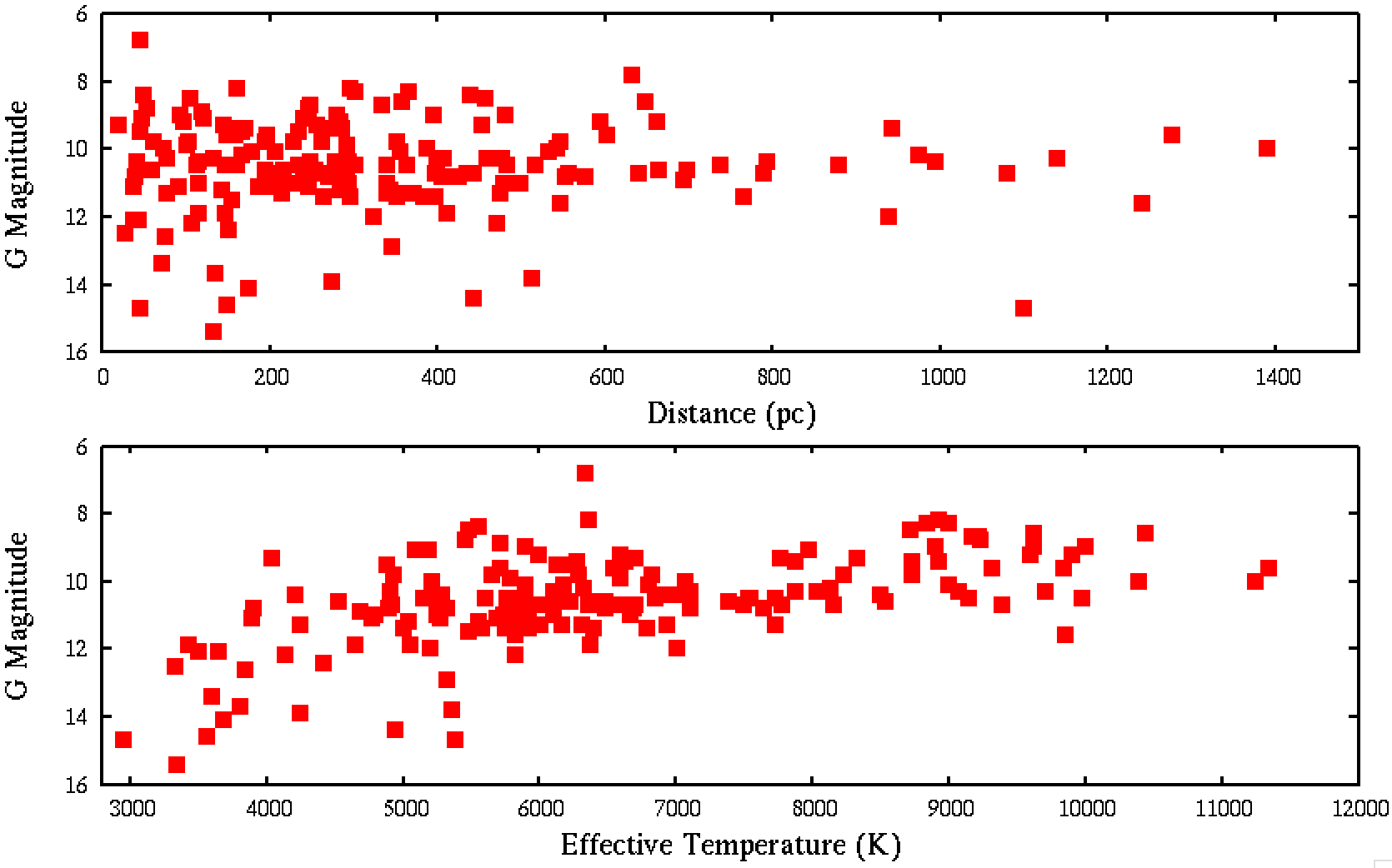
Figure 1: Properties of the TESS stars in our sample using ExoFOP TOI database values. Referenced to the DR2 Gaia apparent magnitude, these plots show the distribution of the distance and effective temperature within the sample. Most stars are near 10-11th magnitude, closer than 500 pc, and cooler than 7000K. A few more distant and hotter stars are not shown (See Table 1).

Table 1 lists the TESS targets we observed and which will be discussed in this paper. In order to characterize each star we list in Table 1 some relevant stellar parameters; the Gaia magnitude, effective temperature of the star, and the Gaia determined distance as obtained from the ExoFOP archive TESS TOI table in October 2020. In all cases, we used the well-vetted “default” or “preferred” stellar parameters as given in the ExoFOP archive. Column 5 gives the date of observation, with the remaining four columns being the 5$\sigma$ $\Delta$mag contrast limit obtained in the observation at 0.2 and 1.0 arcsec in each band-pass.

Gaia parallaxes can be unreliable for close binaries as described in Arenou et al. (2018) with a good discussion related to Gaia parallexs and high-resolution imaging presented in Ziegler et al. (2020). Close binaries resolved by Gaia, usually having separations of 0.7 arcsec or larger, are somewhat large by our standards. For unresolved binaries, Arenou et al. (2018) states “…the astrometric quality of unresolved binaries with a small magnitude difference is not significantly different from that of single stars.” The uncertainties in the Gaia parallax values for resolved close binaries ($\geq$0.7 arcsec) manifest themselves in cases such as faint stars (fainter than G=$\sim$17), crowded sources (leading to duplicate entries), diffuse objects, and nearly resolved binaries spatially close to bright stars. We have six stars in Table 1 (TOIs 523, 1152, 1162, 1163, 1172, and 1393) which fall into the duplicate and crowded/nearby bright star categories (See note to Table 1). Only three of these, those in italics in the above list, revealed a nearby star in our observations which Gaia also resolved. In all three cases, the companions are widely separated from the primary star at 1.5 arcsec. While the distances to these three stars may have a larger than average parallax uncertainty, none of these wide companions are considered in the detailed analysis of this paper nor do they have any effect on its conclusions.

Speckle imaging provides angular resolutions to the diffraction limit of the telescope. For NESSI at WIYN, the inner working angle yields angular resolutions of 39 and 64 mas, providing spatial resolutions of 4-20 au (at 100-500 pc, 562 nm) and 6.2-31 au (at 100-500 pc, 832 nm). Eight of the 186 TESS TOIs presented herein were observed years ago at WIYN, as they were first detected as exoplanet host stars by the Kepler mission. These stars (identifiable in Table 1 by their date of observation) were observed using the Differential Speckle Survey Instrument (DSSI, Horch et al. 2009), which was the speckle imager used at WIYN from 2008 until NESSI was commissioned in 2016. The use of DSSI for exoplanet host star follow-up observations is described in Howell et al. (2011). DSSI used similar filters to NESSI but with slightly different central wavelengths, 692 nm and 880 nm. All observing and reduction procedures were similar to those described above for NESSI.

Figure 1 shows two relevant properties of the TESS targets we have observed in this work, the distance and effective temperature of the sample as a function of the Gaia magnitude. Note that the stars cluster near 10-11th magnitude, 80% are closer than 500 pc, and 75% are cooler than 7000K. The closest stars (d$<$100 pc) represent the faintest and coolest stars in the sample.

Figure 2 shows the contrast range of the observations obtained for our targets as a function of their Gaia magnitude. For each band-pass, we note that the total range in contrast narrows, that is the delta magnitude limits become shallower, as the target star becomes fainter. This is a function of S/N in the Fourier summed images and why our standard observing practice is to use 3 or more images sets per observation depending on the target star magnitude. Seeing too can have a similar effect in lowering the contrast of the final image. While the resolution of speckle imaging does not decrease with bad seeing, spreading the light out over a larger area both decreases the correlation of individual speckles across the image (having a correlation size of about 1 arcsec; Howell et al. 2019) as well as making individual speckles harder to detect above any background sky noise during the 40 ms observation time. Both of these effects will reduce the interferometric signal in the data due to a lowering of the S/N in the final image. For the observations presented here, the majority were observed in seeing of 1.1 arcsec or better.

Examining Figure 2, it can be seen that the 562 nm bandpass keeps approximately the same sensitivity difference ($\sim$1 mag) between 0.2 and 1.0 arcsec over the entire magnitude range providing a contrast limit of 4-5 magnitudes at the bright end and 3-4 magnitudes near G=13. The 832 nm band-pass has deeper contrast limits at both reference angular separations. These observations reach a contrast of 7 magnitudes at the bright end (with a range of 2 magnitudes) and reach a contrast limit near 6 magnitudes with a range of 1 magnitude, near G=13. Even though our EMCCDs have 10% less detector QE at 832 nm vs. 562 nm, the atmospheric effects and speckle correlations for each target star are better at redder wavelengths. Greater contrast limits (up to 8 magnitudes) have been achieved at WIYN by obtaining more sets of speckle images because, to no one’s surprise, the more time spent on a target the better S/N of the observation.

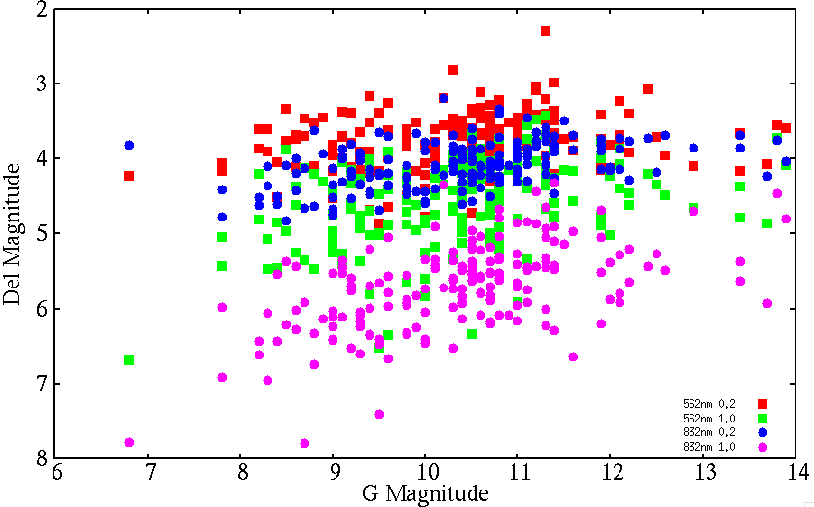
Figure 2: Speckle imaging contrast limits as a function of target star Gaia magnitude. The $\Delta$ magnitude contrast obtained at reference angular separations of 0.2” and 1.0” are shown as a function Gaia magnitude for our TESS sample. Note that the contrast obtained is both larger and extends to greater $\Delta$ magnitudes at 832 nm while both filters show a convergence in overall contrast range toward fainter stars.

3 Detected Companions

As an example of one of our speckle imaging reduced data products, Figure 3 presents typical contrast curves we obtain with NESSI observations at WIYN. The field of view of NESSI in speckle mode (0.018 arcsec/pixel) is 19 X 19 arcsec, however we typically only read out a 256 X 256 pixel subsection region of interest centered on the target star yielding a final image of 4.6 arcsec on a side. However, as mentioned earlier, speckle decorrelation occurs within the atmosphere outside of $\sim$1 arcsec; therefore, we only use the robust Fourier analysis and speckle reconstruction techniques, as well as determine the 5$\sigma$ contrast limits (blue points) and our fit to them (red curve) for an angular size patch of sky of 1.2 arcsec on a side, beyond which decorrelation occurs, becoming worse with increasing separation (Horch et al., 2011). Figure 3, showing the binary exoplanet host star TOI 894, reveals the detected close companion as a “+” sign below the 5$\sigma$ contrast curves as well as displaying the companion star (located to the upper right) in the speckle reconstructed image insets displayed under each curve.

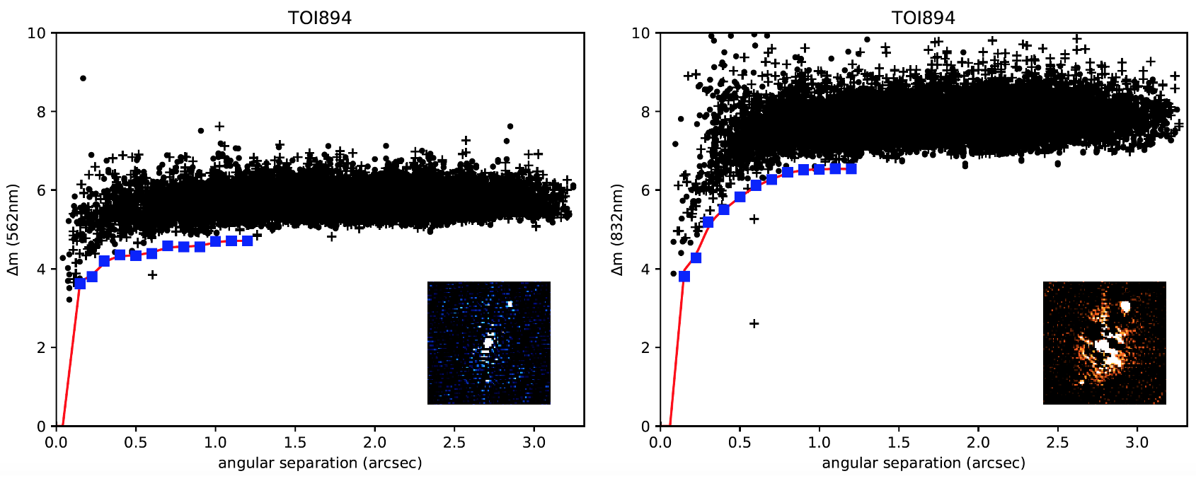
Figure 3: Speckle imaging contrast curves and reconstructed images for TOI 894. The red curve in each plot is a fit to 5$\sigma$ blue points measured at various annuli. The black + signs and filled square symbols are background measurements of the limiting contrast in the reconstructed image; + sign being points above the mean “sky”. Note the detection of the companion star at $\sim$0.5 arcsec separation, well beyond the 5$\sigma$ limit. The companion is also seen in the approximate 1 arcsec square inset images which have N up and E to the left.

Table 2 lists the companion stars we have detected, many seen in both band-passes with fainter and/or redder companions detected only in the 832nm observation. The table gives the target name, angular separation, position angle, and $\Delta$magnitude within each respective band-pass with global internal uncertainties near $\pm$6 mas, $\pm$2 degrees, and $\pm$0.2 magnitudes, respectively. Similar values for “Sep” and “PA” between the two filters provide additional confirmation of the goodness of fit of the Fourier analysis. The last column presents an estimate of the orbital separation of the two stars, in au, using the distance given in Table 1 and assuming that the instantaneous spatial separation detected in our imaging is approximately the orbital semi-major axis. Thirteen stars have companions beyond 1.25 srcsec, four of which, TOI851, TOI944, TOI994, and TOI1162, have fairly wide separated companions in the “speckle world” (well beyond $\sim$1.25 arcsec), thus their $\Delta$mag values will not be as accurate as the rest, perhaps being overestimated and with an additional uncertainty of $\pm$0.5 magnitudes (Howell et al., 2011). Stars with companions within $\sim$30 au will have binary orbital periods of decades and be systems that will reveal orbital motions within only a few years (See Colton et al., 2020 submitted). Two TOIs, 1163 & 1228 are shown to be triple systems having a close companion with a wider tertiary.

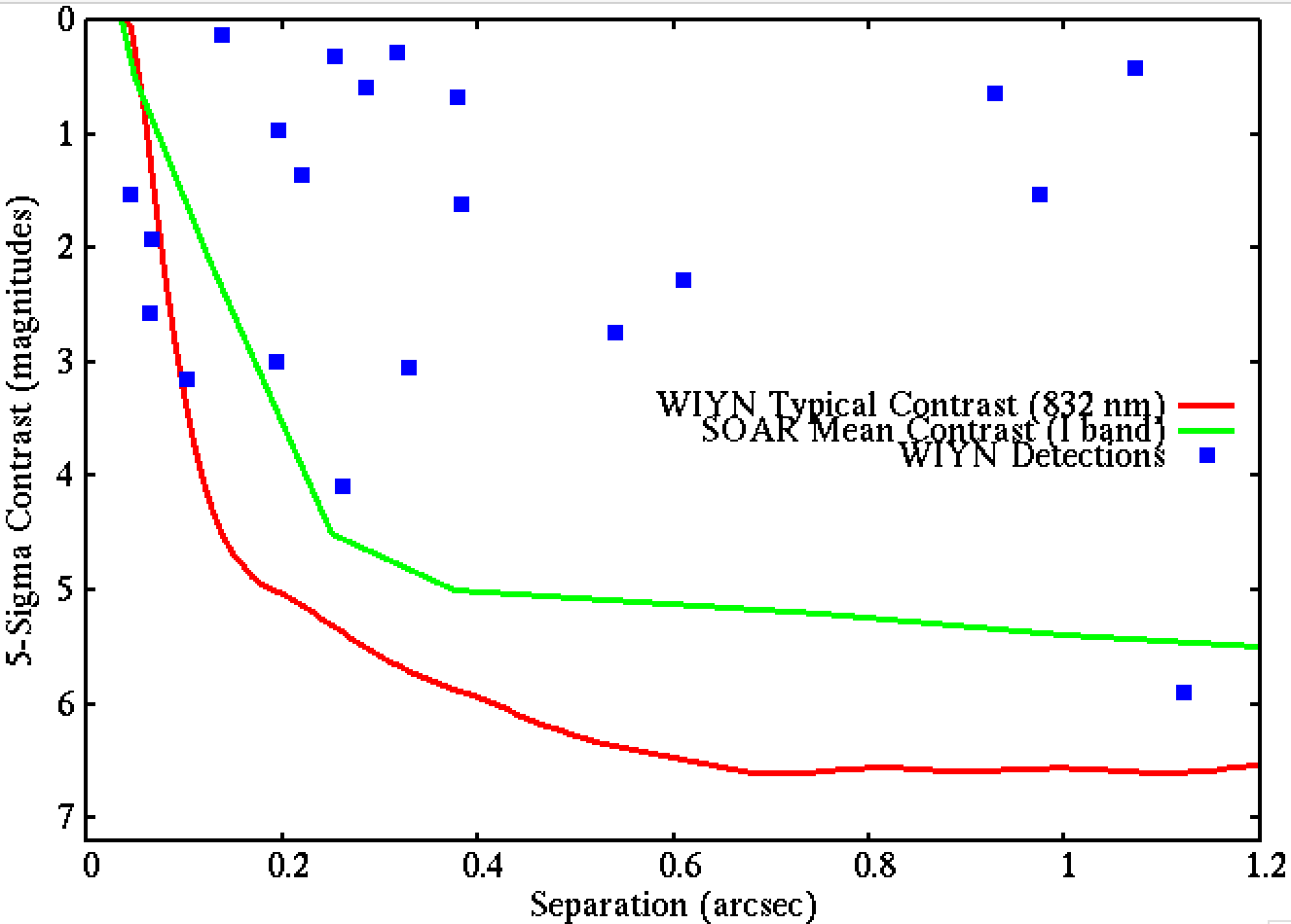
Figure 4: Speckle imaging 5-Sigma mean contrast curves. The SOAR I-band curve is from Ziegler et al. (2020) and the WIYN 832 nm curve is from Scott et al. 2018. The two contrast curves essentially match near the diffraction limit of the telescopes (SOAR is 4.1-m and WIYN is 3.5-m), with the WIYN 832 nm contrast limit being deeper at all separations. The stellar companions detected at WIYN inside 1.2 arcsec are shown including four inside 0.1 arcsec that would not be detected at SOAR.

Ziegler et al. (2020) recently published a paper describing TESS TOIs observed by speckle interferometry at the 4.1-m SOAR telescope in Chile. SOAR and WIYN have similar apertures, so a comparison of any common systems is useful. Not many TOIs were common between the SOAR program and ours at WIYN as TESS surveyed the southern sky in year 1 and the northern sky in year 2. However, five TOIs with detected companions (123, 172, 462, 851, 952) were observed by both telescopes/instruments and in all cases the derived parameters for the detected companions were in complete agreement.

Figure 4 compares the 5$\sigma$ contrast curves for NESSI at WIYN and the speckle imager at SOAR. The curves roughly match near the diffraction limit of these similar size telescopes while the WIYN 832-nm contrast curve limit is deeper at all separations. The companions detected at WIYN inside 1.2 arcsec (the range of good speckle interferometric correlation) are also shown in Figure 4, including four very close companions that would be undetectable at SOAR. These four exoplanet host star bound companions orbit very close to the primary star (35, 35, 16, and 7 au) and contain planetary systems with close-in (periods of 1 to 5 days), Neptune-size (radii of 5 to 9 R_e) planets.

Of the 186 TESS exoplanet host stars (TOIs) discussed in this paper, 45 total companions were found, 36 are within 1.2 arcsec. More interestingly, 21 of the companions are within 0.5 arcsec and 9 are inside 0.25 arcsec - companions difficult to impossible to detect by other means. Our speckle imaging program is aimed at the detection of companions that can cause validation and exoplanet characterization problems and can cause spectral modeling to produce incorrect values for the host star properties (Furlan & Howell, 2020). We are particularly interested in finding true, bound companions, stars that generally lie inside 0.25 arcsec (Matson et al., 2018), which are hard or impossible to discover with other instruments or other means. These true bound companions are the stars which will provide detailed robust information for exoplanet formation, dynamics, and evolution. Finally, our simultaneous two-color observations allow us to not only detect companions, but also gain some astrophysical knowledge for them in terms of the companion spectral type (i.e., mass, see below).

4 Discussion

Speckle interferometry has become one of the leading ground-based telescope follow-up resources in the study of exoplanets. Such observations are critical to obtaining correct stellar and exoplanet properties. While both the Kepler and K2 mission exoplanet host stars yielded a similar percentage of binaries (near 40-50%; Horch et al. (2014); Deacon et al. 2016; Matson et al. 2018; Ziegler et al. 2018), the missions sampled different regions of the sky (single field of view at mid-galactic latitude vs. multiple ecliptic fields of view) as well as having different observing strategies and photometric precision levels.

The TESS survey affords us with an opportunity to directly compare the observed stellar companion detection fractions and binary host star properties for nearly equal surveys in the southern and northern sky. We acknowledge that the speckle interferometric observed companion stars have a bias (as is true of any observational campaign) and do not not represent the full story. The companions that are missing could be those with large magnitude differences (below the contrasts available), orbital locations which place them inside even the resolution of speckle imaging (very close binaries), companions of very red color (very faint in the optical band-pass), and companions at separations outside the field of view (i.e., outside the angular distance for speckle correlation, near 1.2”). In our speckle imaging program, we concentrate on nearby companions ($<$1.2 arcsec), stars with a high probability of being true bound companions and essentially undetectable by other means. In our analysis, we account for possible “missing” companions in a statistically probabilistic manner (see below).

Using $<$1.2 arcsec as a guide, we find that 24 out of our total of 186 stars show a detected companion, giving a detection fraction of 13%. Ziegler et al. (2020) find 67 stars (out of 542 total stars they observed) with detected companions within 1 arcsec or 12.5%. This is gratifying to see as it lends credence to the fact that the exoplanet host stars which are binaries seem to yield the same observed percentage in both hemispheres when using comparable (but different) instruments and telescopes. It is interesting to note that the observed percentage of 13% is roughly twice that seen for Kepler and K2 exoplanet host stars observed with speckle imaging at the WIYN telescope, 7% (Horch et al., 2014) and 6% (Matson et al., 2018), but are not unexpected based on the observed 46% true binary fraction and the generally much closer and brighter stars being observed by TESS. See Matson et al. (2019) and §4.1 below.

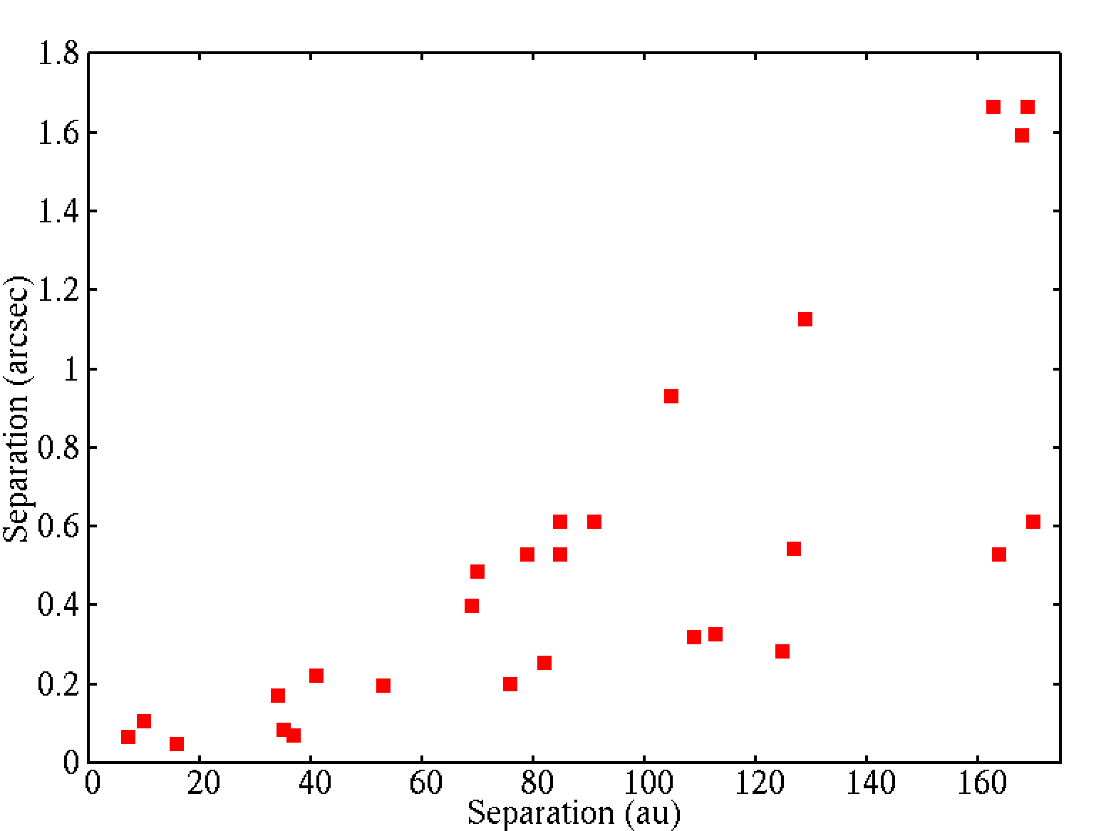
Figure 5: The relationship between angular separation (arcsec) and spatial separation (au) of the detected companions within a projected distance of 200 au (1.6”). We note that the closest spatial separations make up the majority of the closest physical separations. There is a dropoff in the frequency of detected companions outside of $\sim$0.6 arcsec, possibly representing the transition from mostly bound to mostly line-of-sight companions.

Figure 5 shows the relation between the angular separation in arcsec of our detected companions and their projected physical separations in au. We can see in the figure the existence of a near-linear cutoff line for the minimum spatial separation observable as a function of the angular separation available for the TESS targets. Outside of 0.6 arcsec, we see a falloff in the number of detected companions perhaps signaling a true drop-off in bound companions vs. line-of-sight companions (See Matson et al. 2018). Of course, gravitationally bound systems do indeed exist at larger separations than 0.6 arcsec (e.g., Common proper motion pairs), however they are increasingly rare to detect as the separation becomes larger than our field of regard. Using Figure 5, we note that for a typical TESS star ($<$500 pc), the contrast curves in Figure 4 begin to turn over at their inner working angle at values of $\sim$46 au (0.2”) at SOAR and $\sim$14 au (0.1”) with NESSI at WIYN.

4.1 Predictions of Stellar Companions

Matson et al. (2019) used predicted distributions of TESS exoplanet host stars to examine the population of stellar companions detectable with speckle imaging. Here we use the same techniques to compare our observed companions to expectations and estimate the stellar parameters for the companion stars. We begin by considering all possible bound companions for a given TOI using the Modern Mean Dwarf Stellar Color and Effective Temperature Sequence Table based on Pecaut & Mamajek (2013) to assign stars with later spectral types (cooler effective temperatures) as possible companions. For each possible companion we then calculate a $V-$band delta magnitude ($\Delta$m) and mass ratio ($q=M_{2}/M_{1}$) relative to the primary (TOI) star. Because we assign companions based on spectral types, which are discrete and unevenly spaced in mass, we fit a seventh order polynomial to the mass ratios as a function of delta magnitudes for each TOI and then determine the fraction of companions that fall within the 562 nm speckle contrast limit of $\Delta$m $\leq 6$. We also weight the likelihood of each companion by the mass ratio distribution of Raghavan et al. (2010), such that companions with mass ratios of $0.1\leq q\leq 0.95$ are equally likely and those with q $>$ 0.95 are enhanced by 2.5$\times$. Figure 6 shows possible companions for select TOIs, with the spectral type of the TOI indicated by the solid line color and the spectral types of the individual possible companions indicated by the color of the points. The dashed line highlights the speckle detection limit at $\Delta$m = 6, and small vertical lines indicate where the mass ratio is equal to 0.1 for each TOI. The fractions of detectable companions for all TOIs in our sample are listed in Table 3 under “Comp. Frac.”, with a mean of 0.57 for the sample. Table 3 also shows the stellar parameters used in our predictions as well as the spectral type of potential companions at $\Delta$m = 4 and $\Delta$m = 6 for all TOIs observed at WIYN. Two stars without distances are listed for completeness, but no analysis of possible companions is included.

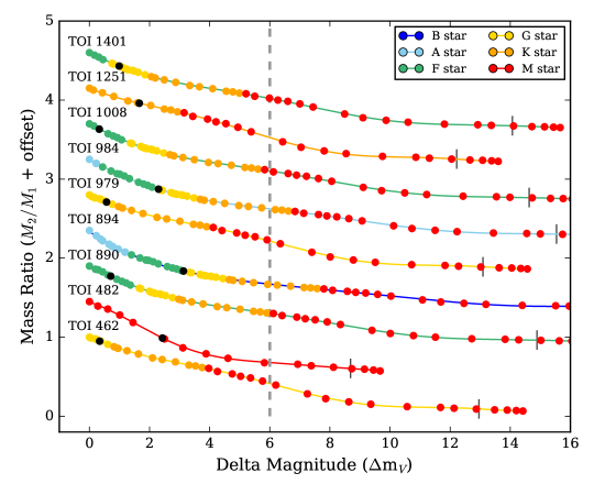
Figure 6: Expected mass ratio (offset for clarity) vs. $V$-band delta magnitude for a sample of TOIs with detected companions. The colors of the lines and dots correspond to the spectral type of the star/possible companion. Contrast limits for speckle imaging at 562nm with NESSI are shown by the dashed line ($\Delta m\lesssim 6$). The small vertical lines along each line indicate where the mass ratio equals 0.1. The black dots show the measured delta magnitude (562nm, except 832 nm used for TOI 482) for observed companions. See the Appendix for a plot of all detected companions.

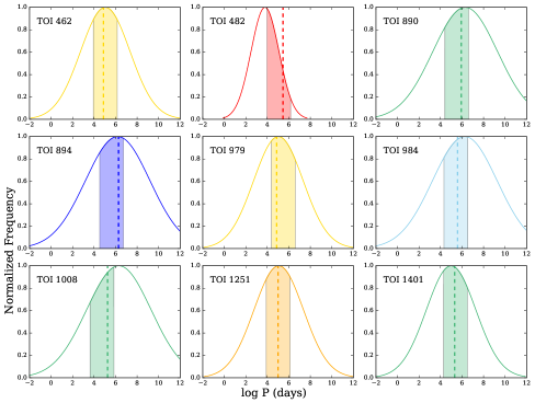
Figure 7: Expected binary period distributions for a selection of TOIs with detected companions based on the distribution presented in Raghavan et al. (2010). The shaded regions (color coded by spectral type of the primary as in Figure 6) show the orbital periods corresponding to projected separations at which speckle imaging at WIYN (562nm) can detect companions. The dashed lines correspond to the separation of observed companions converted to $\log P$ space using the distance and mass of the primary star. See the Appendix for a plot of all binary period distributions.

Since the separation of the components must also be considered when evaluating which companions speckle imaging is sensitive to, we use the binary orbital period distribution for solar-type stars (Raghavan et al., 2010) to determine the fraction of possible companion separations that can be detected. For each TOI we use a log-normal period distribution parameterized by the mean semi-major axis in au and standard deviation in $\log P$ based on the mass of the primary (See Table 3 of Sullivan et al. 2015). The angular resolution limits of NESSI (0.04 - 1.2” at 562nm) are then converted to period space using the mass and distance of each TOI via Kepler’s third law. The binary period distributions and portions of $\log P$ space that are detectable using speckle imaging for TOIs with a range of spectral types are shown in Figure 7 (shaded regions). The speckle limits in au and the fraction of each binary distribution, “Distr. Frac.”, that falls within those limits (converted to $\log P$) are listed in Table 3. The mean “Distr. Frac.” for all TOIs observed at WIYN is 0.34. Taking the mean value for “Distr. Frac.” times the mean value for “Comp. Frac.” (0.57 from above), we should expect to actually observe bound companions around $\sim$19% of our stars, a value comparable to our observed value of 13%.

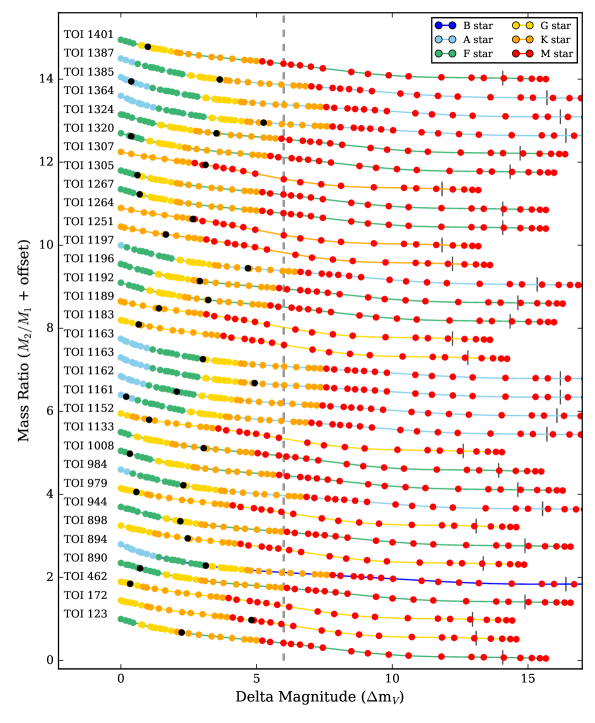
Figure 12: Expected mass ratio (offset for clarity) vs. $V$-band delta magnitude for TOIs with companions detected at 562nm. The colors of the lines and dots correspond to the spectral type of the star/possible companion. Contrast limits for speckle imaging with NESSI are shown by the dashed line ($\Delta m\lesssim 6$). The small vertical lines along each line indicate where the mass ratio equals 0.1. The black dots show the measured delta magnitude of the observed companions.

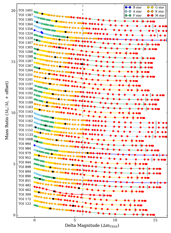
Figure 13: Expected mass ratio (offset for clarity) vs. TESS-band delta magnitude for TOIs with companions detected at 832nm. The colors of the lines and dots correspond to the spectral type of the star/possible companion. Contrast limits for speckle imaging with NESSI are shown by the dashed line ($\Delta m\lesssim 6$). The small vertical lines along each line indicate where the mass ratio equals 0.1. The black dots show the measured delta magnitude of the observed companions.

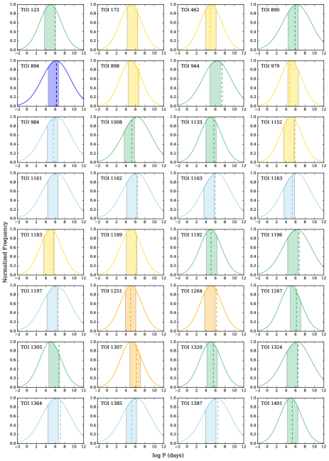
Figure 14: Expected binary period distributions for all TOIs with companions detected in 562nm based on the distribution presented in Raghavan et al. (2010). The shaded regions (color coded by spectral type of the primary as in Figure 6) show the orbital periods corresponding to projected separations at which speckle imaging at WIYN can detect companions ($0.04-1.2"$). The dashed lines correspond to the separation of observed companions converted to $\log P$ space using the distance and mass of the primary star.

Figures 6 and 7 also show where observed companions from this study were detected in relation to our predictions. As in the predictions, we assigned the spectral type of the primary star based on the $T_{\mathrm{eff}}$ reported in Table 1, and then determine the spectral type of the secondary using the observed delta magnitude. For systems with small separations and small delta magnitudes, such as TOI 890, 979, 1008, and 1267, the reported effective temperature will be a combination of both stars. While disentangling the temperatures of the two components in these systems does not impact our overall results, it should be considered for detailed analysis of the individual systems. The 562 nm delta magnitude of companions observed around the TOIs in Figure 6 are shown as black dots (832 nm shown for TOI 482), while the observed separations for the same companions are indicated by dashed lines in Figure 7. Plots showing our predictions and the observed delta magnitudes and separations for all TOIs with detected companions are given in the Appendix (Figures 11-14).

Similar to Figure 4, the plot of delta magnitude vs. mass ratio illustrates that most companions detected at WIYN have $\Delta$mag $\leq 3-4$ and have companions of the same or slightly cooler spectral types. We estimate the mass ratio for each observed system by converting the predicted $V-$band delta magnitude to a TESS delta magnitude (via Stassun et al. 2018) and fitting a polynomial to the possible mass ratios as a function of $\Delta$m_TESS. We then use the observed 832nm $\Delta$m values for each TOI (since all companions were detected in that filter) to determine the mass ratio from the polynomial fit.

A histogram of the mass ratios for all detected companions is shown in Figure 8, with the companions detected within 1.2” shown as hatched bars. The mass ratio distribution shows an increase in the number of high-q systems with a uniform distribution at lower-q, in agreement with Raghavan et al. (2010). The drop off at the lowest q-values ($\leq$0.4) is where our sensitivity to faint, red companions decreases. Figure 8 also shows the mass ratios as a function of separation in au, with the companions detected within 1.2” shown as solid points. While the lack of low-q systems at smaller separations could be taken as an observational bias (and likely is), the relative lack of close ($<$1.2”) high-q systems at larger separations is indeed interesting and suggestive. Similarly, Raghavan et al. (2010) opined that short-period systems prefer higher mass ratios, that is, like-mass pairs (q$>$0.95) prefer relatively short orbital periods. Likewise, Moe & Di Stefano (2017) noted that the “twin fraction” significantly decreases with orbital period. We also see a slight preference for the hotter stars to be in high-q systems whereas the cooler stars tend toward low-q systems.

For the stars shown in Figure 8, we examined in detail possible connections of planet radius or orbital period with the stellar properties. Neither exoplanet orbital period (ranging from $<$1 to 15 days, well within even our closest binary systems at $<$10 au) nor exoplanet radius ($<$1 to 30 R_e) showed a meaningful correlation with the stellar or binary properties in this relatively small sample. Nine of the 25 exoplanets in these binaries are larger than 10R_e and generally belong to wider separated pairs ($>$200 au). TOI 1191 is a notable exception harboring a planet of radius 25.4R_e, orbital period of 15.7 days, and residing in a binary system separated by only 16 au.

Figure 7 confirms that observed companions also fall within our expected separation/period ranges and highlights our sensitivity to the peak of the expected binary period distribution for most TOIs, making speckle imaging ideal for companion searches. While further information is needed to robustly prove whether the observed companions are truly bound, the fact that the delta magnitudes and separations we measure correspond to realistic binary parameters gives us confidence that most close companions are likely to be physically bound.

Figure 8: Left: Calculated mass ratios for all companions detected with speckle imaging at WIYN including those detected within 1.2” (hatched bars). The mass ratios were determined using the measured $\Delta$mag at 832nm and a polynomial fit to the mass ratio as a function of TESS delta magnitude based on Pecaut & Mamajek (2013). See Figure 6 and the text for more details. Right: Mass ratio as a function of separation in au for all companions (open points) and those detected within 1.2” (solid points).

We also use our fraction of possible companions (“Comp. Frac.”) and fraction of each binary period distribution (“Distr. Frac.”) that NESSI can detect to estimate the number of companions we expect to observe around the 186 TOIs observed at WIYN. For each TOI we determine the “Comp. Frac.” and “Distr. Frac.” in separation bins of width=0.01” from 0.04 to 0.24” and bins of width=0.2” from 0.24 to 1.24”, to account for the rapidly changing delta magnitude detection limits at close separations (see Fig. 4). We then multiply the “Comp. Frac.” by the “Distr. Frac.” for each TOI (see “Speckle Frac.” in Table 3), and sum the fraction of companions in each separation bin to determine the total number of companions we expect to detect with speckle imaging. Assuming 46% of the TOIs have true bound companions, we multiply the total number of detectable companions by 0.46 to get $\sim 17$ expected companions within 1.2”. The results are plotted in Figure 9, with the expected number of companions shown in separation bins of 0.2” as yellow bars, and the observed companions within 1.2” plotted as blue-hatched bars. The error bars on the expected companions reflect the minimum and maximum total number of expected companions determined by randomly selecting which 46% of the TOIs have companions for 100,000 random iterations. While our calculations only expect $\sim 17$ companions compared to the 29 we observe within 1.2” of 28 TOIs, the number of companions observed matches the model predictions given the sizable uncertainties in each bin (See Figure 9).

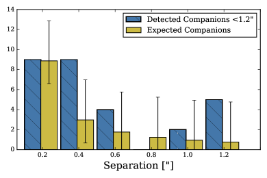
Figure 9: Histogram of companion stars observed within 1.2” of a TOI (hatched blue bars) and the number of expected companions (solid yellow bars) in projected separation bins of 0.2”. The number of expected companions was derived from the fraction of companions that can be detected around 46% of the TOIs using speckle imaging at WIYN. Error bars on the expected companions were determined from the minimum and maximum number of expected companions based on 100000 random combinations of 46% of the TOIs in our sample. See text for more details.

To further examine the population of observed companions and determine whether we see any indication of binary suppression (inside of $\sim$40 au) among close binaries with exoplanets as suggested by Kraus et al. (2016) and Ziegler et al. (2020), we convert the projected separation in arcseconds to au using the distance of each TOI for both the observed and expected companions. Figure 10 shows the separation in au of observed companions within 1.2” in logarithmic bins of 0.5 dex (hatched blue bars).

However, the two left most bins are underrepresented in our sample not due to binary suppression, but due to the speckle contrast curve becoming steep and shallow at small separations. This is a property of every high-resolution imaging instrument, with the inner working angle efficiency falling off at $\sim$14 au at WIYN and $\sim$40 au at SOAR. Given this increased incompleteness at small separations (See Figure 4) we estimate a “correction” factor based on a convolution of the inner contrast curve, that is the steep change in magnitude averaged over the corresponding broad bins in au (taking min au vs. separation as a metric for minimum separations observable at each bin of arcsec, see Fig. 5). This correction increases the left most bins by 0.6 and 2.1 stars, respectively (unfilled hatched bars in Fig. 10). Fitting a Gaussian to the corrected distribution (solid red line) shows that the TESS companion sample peaks at $\sim 100$ au with a width of 0.75 au. The Gaussian distribution was determined using a non-linear least squares fit to the “corrected” bins, but is consistent with the fit determined from a maximum likelihood estimate on the unbinned data.

Figure 10 also shows the expected number of companions (solid yellow bars) based on the Raghavan distribution convolved with the NESSI contrast curve as described previously. A Gaussian fit to the expected companions, using a non-linear least squares fit to the binned data, (solid black line) peaks at a separation of only 26 au, a value biased toward close separations given the NESSI contrast curve convolution with the distribution of Raghavan et al. (2010, peak $\sim$ 50 au, $\sigma$ $\sim$ 1.1). The uncertainties on the expected companion bins, however, allow the distribution to be statistically consistent with the Raghavan distribution, shown in Figure 10 as a dashed yellow line, which has been scaled to the expected number of companions (17) and bin widths.

We also present the unbinned cumulative distribution of detected companions within 1.2 arcsec in Figure 11. The (binned) expected companion distribution from Figure 10 is shown for comparison.

Based on Figures 10 and 11, we note that our distribution of observed companion separations does not match that of Raghavan et al. (2010). While we have only a modest sample of binary exoplanet host star companions, there is evidence in Figures 8-10 that binary stars which host exoplanets have a “Raghavan-like” mass distribution but have a larger mean orbital separation ($\sim$100 au) with a slightly narrower breadth in their distribution. Companion stars can eject planets from stellar systems (Haghighipour, 2006), perturb proto-planetary disks (Jang-Condell, 2015), and create planetesimals through gravitational interactions (Rafikov & Silsbee, 2015). The wider mean separation of exoplanet hosting binaries is likely needed to permit proto-planetary disk formation and planetary evolution without disruption by the stellar companion.

Thus, discussions of close binary star “suppression” might indeed be real, but not because of a fall-off of systems within the Raghavan distribution at close separation period, but rather due to exoplanet host star binaries having a different orbital period distribution all together, one with a larger mean separation.

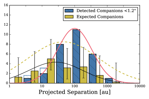
Figure 10: Histogram of projected separation in logarithmic bins of au for companions detected within 1.2” of a TOI at WIYN (solid blue bars). The unfilled hatched bars represent a ‘correction’ factor based on our mean contrast curve range in delta magnitude over the separation bins in au (see Figure 4 and text for more details). A Gaussian fit to the ‘corrected’ companion distributions is shown in red, which is narrower and peaks further out than the distribution of Raghavan et al. (2010). Also plotted is the expected number of companions (solid yellow bars) as determined from the “Comp. Frac.” and “Distr. Frac” of 46% of the TOIs (see text for details). The Gaussian fit to the expected companion distribution is shown in black, while the Raghavan distribution, scaled to the expected number of companions and bin width, is plotted as a yellow dashed line.

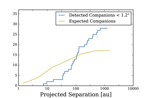
Figure 11: Cumulative distribution for projected separations of companions detected within 1.2” of exoplanet candidate host stars using speckle imaging at WIYN. The expected companion distribution based on the Raghavan distribution convolved with the NESSI contrast curve (see text for details) is shown for comparison. The expected companion distribution is in logarithmic bins of 0.5 dex as in Figure 10. The Y-axis is the number of companions.

5 Conclusion

We have presented the first year of high-resolution speckle imaging observations for TESS stars using the NN-EXPLORE NESSI instrument at the 3.5-m WIYN telescope. Speckle observations of 186 TESS exoplanet host stars were carried out, the majority of which were brighter than 12th magnitude, closer than 500 pc, and solar-like. Of the TESS stars observed, 45 (13%) revealed a close companion. This number is consistent with the expected 19% value based on our models. The distribution of stellar mass ratios in exoplanet binary star systems seems to match that of the Raghavan field binary distribution, perhaps presenting some common aspect of binary star formation, while there may be a lack of high-q binaries at wider separations. Our measured orbital separation distribution, however, does not match the expectation. Our observations support the fact that exoplanet hosting binary stars have, in general, wider separations (longer orbital periods) than field binaries. Thus, the suggested close binary suppression is really not “missing” short period systems from a normal Raghavan-like distribution, but instead is a feature of a wider separation population of binaries, those that host exoplanets.

Additional observations of binary exoplanet host stars are needed in order to build up the sample. A control sample, that is a sample of similar TESS stars not seen to show a transit event, are also needed in order to help vet observational biases. Higher contrast, higher resolution speckle imaging observations will be presented in an upcoming study of TESS exoplanet host stars using 2 years of speckle interferometric observations from the 8-m Gemini North and Gemini-South telescopes.

Note added in Proof: After our analysis was finished and this paper submitted, Gaia EDR3 was released, providing refined parallax values. These improved values, essentially all within $\pm$10% for our stars with companions of 1.2 arcsec or less, produce only small bimodel changes to the distances and are inconsequential in relation to the main results presented in this paper.

Table 1: TESS Stars Observed by NESSI at WIYN

Target	Gaia Mag	Teff	Dist	UT Date	$\Delta$Mag 562 nm		$\Delta$Mag 832 nm
		K	(pc)	MM/DD/YY	0.2”	1.0”	0.2”	1.0”
TOI 103a	11.9	6371	411.2	06/18/19	3.41	3.77	3.82	4.68
TOI 109b	13.8	5361	513.0	06/19/19	3.55	3.72	3.75	4.46
TOI 123	8.2	6356	161.5	06/19/19	3.60	4.20	4.52	6.43
TOI 172	11.2	5759	342.8	06/19/19	3.41	4.04	3.83	5.44
TOI 254	10.3	6101	133.3	01/21/19	2.81	3.98	4.03	6.52
TOI 260	9.3	4049	20.2	01/21/19	3.90	4.82	4.02	6.60
TOI 266	9.9	5784	101.7	01/21/19	3.51	4.62	3.66	6.25
TOI 278	14.7	2950	44.4	10/13/19	3.46	4.23	3.47	4.77
TOI 309c	12.9	5329	345.3	01/24/19	4.10	4.66	3.85	4.69
TOI 316	13.9	4245	275.0	10/12/19	3.59	4.09	4.04	4.80
TOI 329	11.2	5560	284.4	01/23/19	3.09	3.48	3.64	4.43
TOI 390	10.2	6321	167.3	10/12/19	3.19	4.35	3.19	4.35
TOI 438	10.0	5211	72.5	10/10/19	4.40	5.60	4.57	6.46
TOI 461	9.5	4884	45.6	10/12/19	3.39	4.47	3.64	5.66
TOI 462	11.1	5696	205.4	10/10/19	3.83	5.34	3.97	5.49
TOI 482	14.1	3692	173.8	10/11/19	3.34	4.11	3.59	4.62
TOI 484	12.4	4421	150.0	10/11/19	3.08	4.20	3.72	5.44
TOI 488	12.5	3329	27.4	11/18/19	3.71	4.34	4.18	5.26
TOI 493	12.2	4139	107.4	10/14/19	3.40	4.46	4.28	5.64
TOI 503	9.3	7764	255.4	10/14/19	4.15	4.93	4.33	6.24
TOI 509	8.4	5560	49.0	10/14/19	4.05	4.85	4.61	6.44
TOI 515	14.4	4952	442.8	10/14/19	3.26	4.13	3.10	4.43
TOI 518	10.5	5891	159.8	10/14/19	3.61	3.92	4.04	5.62
TOI 523d	9.6	4914	78.0	11/18/19	3.47	3.94	4.17	5.59
TOI 524	10.4	6924	293.3	10/10/19	4.43	4.98	4.60	5.84
TOI 526	13.4	3601	70.9	10/10/19	4.16	4.79	3.85	5.63
TOI 530	14.6	3566	148.8	10/13/19	3.38	4.54	3.71	5.20
TOI 532	13.7	3815	135.0	10/10/19	4.07	4.86	4.23	5.93
TOI 538	15.4	3352	133.2	10/11/19	3.58	3.91	2.72	3.53
TOI 544	10.4	4220	41.1	10/10/19	3.70	4.54	4.44	5.93
TOI 554	6.8	6338	45.6	10/11/19	4.23	6.69	3.82	7.78
TOI 556e	11.9	5056	146.9	10/10/19	4.15	4.89	4.14	5.05
TOI 557	12.6	3841	76.0	10/12/19	3.96	4.49	3.69	5.49
TOI 603	10.1	5901	205.9	11/18/19	3.60	5.18	4.14	5.46
TOI 628	10.1	6174	178.7	10/11/19	3.77	4.49	4.09	5.42
TOI 629	8.7	9165	333.4	10/10/19	3.70	5.36	4.65	7.80
TOI 647	10.8	4900	553.6	11/18/19	3.61	4.41	4.23	5.34
TOI 685f	10.5	5466	213.3	02/05/18	3.79	5.41	3.88	7.52
TOI 692	9.0	9622	482.0	10/13/19	3.81	5.13	4.12	6.11
TOI 693	11.9	4654	114.8	11/17/19	4.03	4.77	3.73	5.51
TOI 727	12.1	3653	43.0	11/18/19	3.68	4.07	4.14	5.80
TOI 774g	11.8	6070	297.5	04/18/16	2.87	3.13	2.82	3.25
TOI 844	12.2	5830	472.3	10/10/19	3.92	4.62	3.76	5.20
TOI 851	11.5	5485	154.5	10/12/19	3.73	4.15	3.49	5.14
TOI 852	11.4	5574	351.4	10/12/19	3.49	4.76	3.70	5.42
TOI 855	11.0	6671	294.4	10/10/19	4.10	4.80	4.00	5.41
TOI 879	9.6	9839	602.7	10/10/19	3.98	4.89	4.19	5.97
TOI 880	9.8	4935	60.7	11/18/19	3.72	4.55	4.48	5.96
TOI 881	10.4	5274	994.7	10/11/19	3.97	4.79	4.20	6.13
TOI 882	10.0	7069	388.0	10/10/19	4.77	5.84	4.59	6.05
TOI 883	9.8	5651	102.6	10/13/19	3.75	4.33	4.25	6.32
TOI 884	10.0	11246	1390.5	10/11/19	3.81	4.86	3.89	5.34
TOI 885	10.9	4692	693.4	11/18/19	3.52	4.15	4.08	6.08
TOI 886	8.3	8844	364.9	10/13/19	3.61	5.07	4.36	6.95
TOI 888	9.8	6822	263.0	10/10/19	4.49	5.66	4.23	5.87
TOI 890	11.3	6935	474.6	11/18/19	3.45	4.12	3.66	4.64
TOI 892	11.3	7723	340.5	11/10/19	3.96	4.67	3.96	5.37
TOI 893	11.6	9856	1241.4	10/13/19	3.71	4.57	3.88	6.64
TOI 894	9.2	9900	661.7	10/13/19	3.79	4.67	4.23	6.53
TOI 895	9.2	5998	96.3	10/11/19	3.38	4.33	3.80	5.59
TOI 896	9.4	6627	156.1	10/10/19	4.68	5.81	4.48	6.34
TOI 897	9.5	6128	165.9	10/11/19	4.18	5.02	4.19	6.47
TOI 898	11.0	5895	479.1	11/18/19	3.65	4.26	3.77	5.26
TOI 938	11.3	5981	215.0	10/12/19	3.48	4.36	3.58	5.32
TOI 939	11.3	6160	352.2	10/12/19	3.49	4.35	3.76	5.45
TOI 941	11.4	5920	263.4	10/10/19	3.66	4.59	4.46	6.29
TOI 943	11.4	6794	397.8	10/10/19	4.20	4.78	4.26	5.48
TOI 944	12.0	7011	938.4	10/10/19	4.13	5.02	4.15	5.38
TOI 950	10.7	6706	211.6	10/10/19	4.30	5.12	4.11	5.82
TOI 952	10.3	7110	459.2	10/12/19	3.64	4.64	3.68	5.36
TOI 957	9.0	8897	280.2	10/10/19	4.16	5.04	4.52	6.42
TOI 958	11.4	5745	297.1	10/11/19	2.98	3.89	3.91	4.90
TOI 959	10.7	7491	639.6	10/13/19	3.67	4.70	4.20	6.20
TOI 960	10.7	9385	789.9	11/18/19	4.00	4.48	3.82	5.18
TOI 961	11.1	5924	246.2	10/13/19	3.48	4.40	4.07	5.46
TOI 963	11.1	5815	203.9	10/13/19	3.27	4.35	3.93	5.91
TOI 965	11.0	6110	224.5	11/18/19	3.56	4.05	3.85	5.66
TOI 969	11.3	4249	77.3	10/13/19	2.30	4.20	4.08	6.23
TOI 971	11.0	5743	229.6	11/18/19	3.45	3.95	4.14	6.16
TOI 973	11.9	3435	4153.0	11/18/19	3.73	4.00	3.89	6.20
TOI 977	11.3	6307	6862.4	10/11/19	3.20	4.28	4.20	6.01
TOI 978	10.7	6368	291.6	11/18/19	4.15	5.04	4.25	5.83
TOI 979	10.8	5806	414.9	11/18/19	3.96	4.50	3.71	5.03
TOI 980	10.8	5322	269.6	11/18/19	3.92	4.57	4.27	5.59
TOI 982	10.4	8502	793.4	11/18/19	3.59	4.12	3.95	5.49
TOI 984	10.7	7773	442.8	11/18/19	3.78	4.76	4.08	5.71
TOI 985	10.7	6003	260.6	10/14/19	3.28	4.23	4.22	5.51
TOI 986	10.3	8031	407.5	10/13/19	3.57	4.69	3.83	5.73
TOI 989	10.3	7875	476.8	10/11/19	3.99	5.35	3.90	5.98
TOI 994	10.0	10393	543.1	11/18/19	4.06	4.81	3.78	5.73
TOI 995	10.7	4920	1080.9	10/11/19	3.85	4.99	4.25	6.17
TOI 1002	9.4	8924	943.1	11/18/19	3.17	4.01	4.14	6.36
TOI 1007	9.2	6596	283.3	11/18/19	3.40	4.15	4.16	5.69
TOI 1008	9.3	6699	144.3	10/11/19	3.96	5.37	3.94	6.17
TOI 1012	8.2	8928	296.0	10/14/19	3.87	4.81	4.62	6.61
TOI 1132	9.4	7880	286.7	10/14/19	3.90	4.70	4.44	5.99
TOI 1133	9.5	6244	233.4	10/14/19	4.86	6.52	4.68	7.41
TOI 1134	9.4	6277	170.7	10/11/19	4.18	5.02	4.24	5.20
TOI 1138	9.0	9994	395.1	10/11/19	4.53	5.25	4.67	5.53
TOI 1144h	9.2	4777	37.8	06/13/11	4.02	6.27	3.84	4.71
TOI 1145	8.4	12433	438.4	10/11/19	4.51	5.46	4.50	5.54
TOI 1149	7.8	13079	632.6	10/14/19	4.16	5.44	4.77	6.91
TOI 1152i	8.5	5485	105.7	11/16/19	3.76	4.97	4.83	6.21
TOI 1159	9.9	6592	292.8	10/10/19	4.16	4.95	4.44	5.83
TOI 1161j	10.4	7986	500	06/22/20	2.96	4.67	3.31	4.34
TOI 1162k	9.8	8730	352.0	10/15/19	3.60	4.71	4.09	5.91
TOI 1163l	9.6	9311	148.7	10/14/19	4.64	6.35	4.36	6.67
TOI 1170	10.5	7734	880.1	10/10/19	3.83	4.41	4.56	5.50
TOI 1171	10.5	7550	482.8	10/12/19	4.72	6.34	4.25	5.49
TOI 1175	10.6	6229	216.5	10/11/19	3.95	4.77	4.38	5.59
TOI 1178	11.1	3897	36.7	10/10/19	3.77	4.34	4.29	5.74
TOI 1181	10.5	6122	302.8	10/14/19	3.69	4.29	3.59	5.09
TOI 1183	10.5	5599	112.9	10/11/19	3.74	4.16	3.86	5.18
TOI 1184	10.6	4534	58.6	10/10/19	3.66	4.27	4.38	5.80
TOI 1189m	10.4	5287	248.6	10/15/19	4.11	5.12	4.31	5.44
TOI 1191	10.1	6800	355.8	10/11/19	3.87	4.75	3.78	4.90
TOI 1192	10.8	6479	283	10/12/19	3.91	4.92	4.09	5.31
TOI 1195	11.0	5246	500.0	10/12/19	4.09	5.91	4.20	5.95
TOI 1196	10.8	6689	424.4	10/15/19	3.31	5.07	3.94	5.53
TOI 1197	10.8	7649	405.6	10/15/19	4.31	5.20	4.32	6.08
TOI 1201	12.1	3506	37.9	11/10/19	3.81	4.40	3.86	5.91
TOI 1235	10.8	3912	39.6	10/14/19	3.22	4.07	4.04	5.61
TOI 1237n	10.6	6212	243.3	06/24/10	4.07	4.96	3.67	4.34
TOI 1241o	11.6	5826	546.5	11/18/19	3.89	4.16	3.69	4.97
TOI 1251	11.1	5273	186.0	11/09/19	3.37	3.56	3.45	4.84
TOI 1263	9.1	5098	46.6	11/16/19	3.37	4.05	4.00	5.53
TOI 1264	11.2	5040	141.8	11/16/19	3.03	3.78	3.76	4.86
TOI 1265p	10.4	6532	341.1	06/13/11	3.96	5.71	2.76	3.15
TOI 1267q	11.9	6378	980	10/25/10	2.46	3.46	2.28	3.30
TOI 1287	9.0	5891	92.7	11/18/19	3.94	4.42	4.75	6.41
TOI 1288	10.4	6180	114.9	11/17/19	3.52	4.37	4.01	5.84
TOI 1290r	9.9	5875	144.2	06/20/10	2.62	4.36	3.32	5.60
TOI 1301	11.1	4781	90.9	11/09/19	3.44	3.73	3.86	5.45
TOI 1305s	10.6	5267	664.4	11/16/19	3.38	3.95	4.11	5.03
TOI 1306	10.5	5273	364.5	11/09/19	3.34	3.66	4.32	5.55
TOI 1307t	11.4	5010	765.3	11/18/19	3.76	4.25	3.82	5.10
TOI 1311	10.7	8153	556.8	11/18/19	3.95	4.57	4.03	5.53
TOI 1314	10.5	5155	285.4	11/17/19	3.59	4.17	4.23	5.37
TOI 1315	9.3	8321	453.7	11/17/19	4.00	4.27	4.34	6.05
TOI 1316	10.7	6556	435.0	11/18/19	3.47	4.03	4.50	5.89
TOI 1317	10.6	8542	697.1	11/17/19	3.11	4.10	4.11	5.56
TOI 1320u	10.4	6500	340.3	11/17/19	3.71	4.08	3.94	4.85
TOI 1321	10.3	9067	1139.3	11/17/19	3.68	4.05	4.08	5.24
TOI 1323	8.3	9003	301.4	11/09/19	3.91	5.48	4.10	6.06
TOI 1324	10.5	6854	339.7	11/17/19	3.61	4.08	3.90	5.63
TOI 1327	8.5	8715	457.8	11/16/19	3.34	3.88	4.08	5.37
TOI 1328	10.7	6585	397.9	11/17/19	3.42	4.15	4.13	5.37
TOI 1329	10.5	7537	398.6	11/17/19	3.69	3.96	4.20	5.54
TOI 1334	9.6	11348	1276.3	11/18/19	3.95	4.21	4.35	5.57
TOI 1339	8.8	5461	53.6	11/18/19	3.51	4.20	4.63	6.33
TOI 1342v	10.8	5869	–	11/18/19	3.83	4.24	3.34	4.78
TOI 1353	10.3	9706	464.2	11/17/19	3.60	4.42	4.10	5.62
TOI 1354	8.8	9224	245.8	11/09/19	4.10	5.48	3.62	6.75
TOI 1355	8.7	9218	248.1	11/09/19	3.47	4.13	4.12	5.92
TOI 1356	9.0	12308	4772.6	11/09/19	3.89	4.75	4.34	6.03
TOI 1357	10.6	7387	254.4	11/17/19	3.68	4.12	3.87	5.79
TOI 1358	8.6	10445	356.7	11/09/19	3.68	4.37	4.19	5.43
TOI 1360	10.1	8999	533.6	11/18/19	4.00	4.25	4.40	5.35
TOI 1362	10.2	8129	975.5	11/17/19	3.55	4.15	4.22	5.72
TOI 1364	9.2	9598	595.3	11/18/19	4.11	4.59	4.53	5.76
TOI 1366	8.9	5717	118.6	11/10/19	3.45	4.30	3.93	6.13
TOI 1367	9.6	6550	195.9	11/10/19	3.62	4.41	4.01	5.79
TOI 1368	9.6	5717	158.2	11/16/19	3.25	3.90	3.70	5.04
TOI 1369	10.5	9139	516.3	11/09/19	3.67	3.96	4.23	4.95
TOI 1370	9.4	8728	275.5	11/09/19	3.52	4.13	4.15	5.70
TOI 1376	10.7	6026	240.0	11/17/19	3.59	4.03	4.09	5.88
TOI 1378	9.8	8224	547.4	11/09/19	3.83	4.18	4.26	5.55
TOI 1381	10.5	9976	737.1	11/17/19	3.80	4.10	4.19	5.20
TOI 1384	10.5	5773	235.2	11/17/19	3.82	4.15	4.20	5.53
TOI 1385w	–	–	324.3	11/09/19	3.82	4.23	4.11	5.87
TOI 1386	10.5	5769	146.9	11/17/19	3.64	4.30	3.99	5.44
TOI 1387	9.1	7976	239.7	11/09/19	3.71	5.26	3.97	6.11
TOI 1391	11.0	5256	115.7	11/17/19	3.75	4.30	4.31	5.71
TOI 1393x	10.4	7000	278.8	11/17/19	3.67	4.19	4.44	5.73
TOI 1394	9.8	6294	195.0	11/17/19	3.67	4.25	4.44	6.34
TOI 1397	10.6	6357	195.0	11/17/19	3.32	3.98	4.08	6.08
TOI 1398	8.6	9623	648.4	11/09/19	4.11	5.25	4.42	6.28
TOI 1399	10.6	6483	252.4	11/09/19	3.47	3.86	4.21	5.22
TOI 1400	11.3	6004	370.8	11/18/19	3.40	3.68	4.06	5.05
TOI 1401	11.4	6403	383.2	11/18/19	3.36	4.25	3.83	4.32
TOI 1402	10.8	7111	576.7	11/18/19	3.31	3.74	4.10	4.67
TOI 1405y	9.1	5195	–	11/09/19	3.70	4.05	4.30	5.36
TOI 1407z	8.1	6129	80.9	09/28/15	3.06	3.97	2.97	3.92
TOI 1554aa	11.5	5497	194	09/17/10	2.95	4.36	3.48	4.85
TOI 1905ab	11.2	4251	64.7	04/11/17	3.67	3.97	4.19	6.05
TIC125192758	14.7	5384	1100.5	11/17/19	3.71	4.11	3.78	4.31

Table 2: TESS Stars with Close Companions

	562 nm			832 nm
Target	Sep (”)	PA (deg)	$\Delta$Mag	Sep (”)	PA (deg)	$\Delta$Mag	Sep (au)
TOI 123	1.296	295.06	2.24	1.285	294.96	1.96	212
TOI 172	1.116	320.59	4.81	1.116	320.59	4.81	383
TOI 309	–	–	–	0.326	74.7	2.31	112.9
TOI 462	0.167	197.15	0.34	0.169	196.37	0.54	34
TOI 482	–	–	–	0.398	267.34	2.43	69
TOI 851	–	–	–	1.839	255.39	5.53	646
TOI 890	0.424	146.69	0.71	0.423	146.65	0.67	201
TOI 894	0.592	331.11	3.13	0.596	330.87	2.41	394
TOI 898	1.291	37.49	2.46	1.289	36.23	2.28	618
TOI 944	2.025	112.78	2.19	2.006	112.48	1.96	1882
TOI 952	–	–	–	1.162	135.34	4.74	534
TOI 979	0.084	241.02	0.57	0.084	239.97	0.55	35
TOI 984	0.281	187.29	2.30	0.283	186.51	2.15	125
TOI 994	–	–	–	1.371	301.43	6.59	745
TOI 1008	0.487	129.85	0.33	0.484	129.70	0.33	70
TOI 1133	0.548	103.305	3.05	0.542	102.810	2.75	127
TOI 1152	1.587	165.670	1.04	1.593	165.311	0.73	168
TOI 1161	1.144	279.7	0.195	1.144	279.7	0.140	572
TOI 1162	1.466	132.344	2.11	1.463	132.078	1.40	516
TOI 1163c	1.671	114.622	4.93	1.662	114.146	3.83	248
TOI 1163c	0.614	216.892	3.02	0.611	215.724	2.28	91
TOI 1183	0.933	225.474	0.66	0.929	224.297	0.65	105
TOI 1189	0.975	319.317	1.40	0.975	319.123	1.54	242
TOI 1191	–	–	–	0.046	323.172	1.54	16
TOI 1192	0.181	200.617	3.22	0.194	201.073	3.00	53
TOI 1196	1.674	199.730	2.91	1.680	198.751	2.27	712
TOI 1197	1.609	26.153	4.68	1.597	25.054	3.83	650
TOI 1241	–	–	–	0.067	320.252	1.92	37
TOI 1251	0.219	251.551	1.66	0.221	250.112	1.36	41
TOI 1264	1.903	313.670	2.65	1.896	313.544	1.82	269
TOI 1267	0.287	144.0	0.69	0.287	144.0	0.594	281
TOI 1287	–	–	–	0.104	346.121	3.16	10
TOI 1288b	–	–	–	1.123	289.478	5.90	129
TOI 1288b	–	–	–	0.065	312.561	2.57	7
TOI 1305	1.080	234.860	0.61	1.073	233.790	0.42	715
TOI 1307	0.337	32.769	3.12	0.330	34.734	3.05	255
TOI 1320	0.321	49.544	0.38	0.319	48.485	0.29	109
TOI 1324c	1.488	194.209	3.52	1.480	187.164	3.11	504
TOI 1342b	0.377	163.202	0.76	0.380	162.798	0.68	355a
TOI 1356	–	–	–	0.263	288.715	4.10	1255
TOI 1364	2.375	110.736	5.26	2.363	110.751	3.85	1410
TOI 1385	0.252	187.738	0.38	0.254	187.044	0.32	82
TOI 1387c	2.274	344.009	3.64	2.319	345.589	2.71	550
TOI 1401	0.200	45.363	0.99	0.197	43.253	0.96	76
TOI 1405	0.386	42.201	1.42	0.385	40.538	1.62	377a

Table 3: Stellar parameters and companion space observable with speckle imaging

TOI	$T_{\mathrm{eff}}$	$V$	$TESS$	D	SpTa	$M_{\mathrm{interp}}$b	Companion SpT at:		Comp.	Min Sep	Max Sep	Distr.	Speckle
	$(K)$	(mag)	(mag)	(pc)		($M_{\sun}$)	$\Delta m_{v}=4$	$\Delta m_{v}=6$	Frac.	(AU)	(AU)	Frac.	Frac.
TOI 103	6371	12.43	11.52	411.21	F6V	1.241	K5V	M1V	0.569	16.62	493.45	0.362	0.206
TOI 109	5361	14.05	13.24	513.01	G9V	0.928	M0.5V	M3V	0.522	20.73	615.61	0.358	0.187
TOI 123	6356	8.32	7.88	161.5	F6V	1.257	K5V	M1V	0.569	6.53	193.8	0.368	0.21
TOI 172	5759	11.3	10.74	342.83	G2V	1.015	K9V	M2.5V	0.514	13.85	411.4	0.365	0.188
TOI 254	6101	10.26	9.83	133.31	F9V	1.101	K6V	M1.5V	0.557	5.39	159.97	0.366	0.204
TOI 260	4049	9.9	8.5	20.19	K7V	0.645	M3.5V	M4.5V	0.589	0.82	24.22	0.376	0.222
TOI 266	5784	10.07	9.46	101.69	G2V	0.997	K9V	M2.5V	0.514	4.11	122.03	0.362	0.186
TOI 278	2950	16.45	13.17	44.4	M5.5V	0.096	M9V	M9V	1.0	1.79	53.28	0.884	0.884
TOI 309	5407	13.06	12.33	345.29	G9V	0.923	M0.5V	M3V	0.522	13.95	414.35	0.365	0.191
TOI 316	4245	14.38	13.12	275.02	K6V	0.684	M3V	M4.5V	0.571	11.11	330.02	0.395	0.226
TOI 329	5560	11.26	10.69	284.39	G6V	0.968	M0V	M2.5V	0.515	11.49	341.27	0.367	0.189
TOI 390	6321	10.33	9.89	167.31	F6V	1.175	K5V	M1V	0.569	6.76	200.77	0.368	0.21
TOI 438	5210	10.24	9.45	72.46	K1V	0.85	M1V	M3V	0.53	2.93	86.96	0.355	0.188
TOI 461	4884	9.78	8.87	45.56	K3V	0.791	M2V	M3.5V	0.548	1.84	54.67	0.41	0.225
TOI 462	5695	11.66	10.66	205.37	G4V	0.995	M0V	M2.5V	0.511	8.3	246.44	0.369	0.189
TOI 482	3692	14.94	13.08	173.82	M1V	0.525	M4.5V	M5.5V	0.677	7.02	208.58	0.411	0.278
TOI 484	4421	12.64	11.69	149.95	K5V	0.711	M3V	M4V	0.568	6.06	179.94	0.414	0.235
TOI 488	3329	13.74	11.2	27.36	M3.5V	0.359	M5.5V	M7V	0.866	1.11	32.84	0.604	0.523
TOI 493	4139	12.55	11.45	107.36	K7V	0.654	M3.5V	M4.5V	0.589	4.34	128.83	0.419	0.247
TOI 503	7764	9.4	9.2	255.42	A7V	1.695	K1V	K6V	0.551	10.32	306.5	0.266	0.147
TOI 509	5560	8.58	7.93	48.97	G6V	0.968	M0V	M2.5V	0.515	1.98	58.77	0.342	0.176
TOI 515	4952	14.49	13.8	442.8	K2V	0.803	M1.5V	M3.5V	0.539	17.89	531.36	0.361	0.194
TOI 518	5891	10.9	10.14	159.81	G1V	1.048	K8V	M2V	0.52	6.46	191.78	0.368	0.191
TOI 523	4692	10.71	9.58	70.65	K4V	0.744	M2.5V	M4V	0.566	2.85	84.78	0.418	0.236
TOI 524	6923	10.47	10.09	293.27	F1V	1.459	K3V	K9V	0.561	11.85	351.92	0.269	0.151
TOI 526	3601	14.31	12.31	70.93	M1.5V	0.506	M4.5V	M5.5V	0.696	2.87	85.12	0.539	0.375
TOI 530	3566	15.4	13.53	148.76	M2V	0.487	M4.5V	M5.5V	0.703	6.01	178.51	0.436	0.306
TOI 532	3815	14.41	12.68	135.05	M0.5V	0.568	M4V	M5V	0.653	5.46	162.06	0.451	0.295
TOI 538	3352	16.54	14.15	133.21	M3V	0.363	M5V	M6.5V	0.762	5.38	159.85	0.453	0.345
TOI 544	4220	10.78	9.65	41.12	K6V	0.677	M3V	M4.5V	0.571	1.66	49.34	0.407	0.232
TOI 554	6337	6.91	6.44	45.62	F6V	1.3	K5V	M1V	0.569	1.84	54.74	0.339	0.193
TOI 556	5055	12.18	11.31	146.9	K2V	0.803	M1.5V	M3.5V	0.539	5.94	176.29	0.367	0.198
TOI 557	3841	13.34	11.64	75.96	M0V	0.542	M4V	M5V	0.614	3.07	91.15	0.531	0.326
TOI 603	5900	10.31	9.74	205.92	G0V	1.075	K7V	M2V	0.524	8.32	247.11	0.369	0.193
TOI 628	6174	10.11	9.66	178.68	F8V	1.264	K6V	M1.5V	0.57	7.22	214.42	0.369	0.21
TOI 629	9165	8.74	8.69	333.38	A1V	2.138	G8V	K4V	0.533	13.47	400.05	0.272	0.145
TOI 647	4900	11.15	10.23	553.63	K3V	0.792	M2V	M3.5V	0.548	22.37	664.35	0.359	0.196
TOI 685	5466	10.61	9.96	213.28	G8V	0.931	M0.5V	M3V	0.515	8.62	255.94	0.369	0.19
TOI 692	9622	9.02	9.02	481.97	A0V	2.284	G5V	K4V	0.531	19.47	578.36	0.278	0.148
TOI 693	4654	12.0	11.22	114.76	K4V	0.749	M2.5V	M4V	0.566	4.64	137.72	0.418	0.236
TOI 727	3653	12.68	11.0	42.97	M1.5V	0.495	M4.5V	M5.5V	0.696	1.74	51.57	0.585	0.407
TOI 774	6070	11.75	11.35	297.46	F9V	1.114	K6V	M1.5V	0.557	12.02	356.95	0.367	0.204
TOI 844	5829	12.12	11.8	472.3	G1V	1.05	K8V	M2V	0.52	19.08	566.76	0.359	0.187
TOI 851	5485	11.31	11.0	154.48	G8V	0.814	M0.5V	M3V	0.515	6.24	185.37	0.368	0.19
TOI 852	5574	11.64	10.95	351.43	G6V	0.969	M0V	M2.5V	0.515	14.2	421.71	0.365	0.188
TOI 855	6671	11.18	10.65	294.42	F4V	1.288	K4V	M0.5V	0.57	11.9	353.3	0.367	0.209
TOI 879	9839	9.55	9.53	602.73	A0V	2.318	G5V	K4V	0.531	24.35	723.27	0.281	0.149
TOI 880	4935	10.1	9.26	60.67	K3V	0.813	M2V	M3.5V	0.548	2.45	72.8	0.349	0.191
TOI 881	5274	10.64	9.79	994.73	K0V	0.868	M1V	M3V	0.528	40.19	1193.68	0.336	0.177
TOI 882	7069	10.07	9.74	387.97	F1V	1.517	K3V	K9V	0.561	15.68	465.56	0.275	0.154
TOI 883	5651	9.96	9.37	102.64	G5V	0.998	M0V	M2.5V	0.509	4.15	123.16	0.363	0.185
TOI 884	11246	9.91	9.95	1390.0	B9V	3.171	G1V	K3V	0.519	56.17	1668.0	0.287	0.149
TOI 885	4692	11.46	10.18	693.39	K4V	0.744	M2.5V	M4V	0.566	28.02	832.07	0.344	0.195
TOI 886	8844	8.34	8.27	364.93	A2V	2.051	G8V	K5V	0.539	14.75	437.91	0.274	0.148
TOI 888	6822	10.02	9.53	263.02	F2V	1.441	K3V	M0V	0.563	10.63	315.63	0.267	0.15
TOI 890	6935	11.14	10.94	474.56	F1V	1.481	K3V	K9V	0.561	19.18	569.48	0.278	0.156
TOI 892	7723	11.43	10.97	340.54	A7V	1.566	K1V	K6V	0.551	13.76	408.65	0.272	0.15
TOI 893	9856	11.92	11.48	1241.42	A0V	2.32	G5V	K4V	0.531	50.16	1489.7	0.287	0.152
TOI 894	9900	9.11	9.17	661.74	A0V	2.325	G5V	K4V	0.531	26.74	794.09	0.282	0.15
TOI 895	5998	9.35	8.8	96.3	F9V	1.104	K6V	M1.5V	0.557	3.89	115.57	0.361	0.201
TOI 896	6627	9.48	9.09	156.14	F4V	1.331	K4V	M0.5V	0.57	6.31	187.37	0.368	0.21
TOI 897	6128	9.74	9.11	165.94	F8V	1.167	K6V	M1.5V	0.57	6.71	199.13	0.368	0.21
TOI 898	5895	10.83	10.57	479.08	G1V	1.074	K8V	M2V	0.52	19.36	574.9	0.359	0.187
TOI 938	5981	11.39	10.85	215.03	F9V	1.063	K6V	M1.5V	0.557	8.69	258.04	0.369	0.206
TOI 939	6159	11.35	10.93	352.2	F8V	1.176	K6V	M1.5V	0.57	14.23	422.63	0.365	0.208
TOI 941	5920	11.46	11.0	263.39	G0V	1.098	K7V	M2V	0.524	10.64	316.06	0.368	0.193
TOI 943	6794	11.2	11.04	397.79	F2V	1.392	K3V	M0V	0.563	16.07	477.35	0.363	0.204
TOI 944	7011	11.99	11.38	938.4	F1V	1.492	K3V	K9V	0.561	37.92	1126.08	0.285	0.16
TOI 950	6706	11.12	10.21	211.59	F3V	1.384	K4V	M0V	0.564	8.55	253.91	0.369	0.208
TOI 952	7110	10.37	10.07	459.16	F1V	1.536	K3V	K9V	0.561	18.55	550.99	0.277	0.156
TOI 957	8897	9.04	8.96	280.19	A2V	2.058	G8V	K5V	0.539	11.32	336.23	0.268	0.145
TOI 958	5745	11.43	10.96	297.12	G2V	1.008	K9V	M2.5V	0.514	12.01	356.54	0.367	0.189
TOI 959	7491	10.85	10.65	639.56	A8V	1.67	K2V	K7V	0.555	25.84	767.48	0.282	0.157
TOI 960	9385	10.58	10.67	789.89	A1V	2.257	G8V	K4V	0.533	31.92	947.87	0.284	0.152
TOI 961	5924	11.46	10.66	246.18	G0V	1.138	K7V	M2V	0.524	9.95	295.41	0.368	0.193
TOI 963	5814	11.0	10.64	203.87	G2V	1.039	K9V	M2.5V	0.514	8.24	244.65	0.369	0.19
TOI 965	6110	11.1	10.61	224.49	F8V	1.141	K6V	M1.5V	0.57	9.07	269.39	0.369	0.21
TOI 969	4249	11.65	10.54	77.26	K6V	0.685	M3V	M4.5V	0.571	3.12	92.71	0.419	0.239
TOI 971	5743	11.17	10.52	229.6	G3V	1.008	K9V	M2.5V	0.512	9.28	275.51	0.369	0.189
TOI 973	3435	13.69	10.58	4153.0	M3V	0.401	M5V	M6.5V	0.762	167.81	4983.6	0.041	0.032
TOI 977	6307	11.62	10.52	6862.39	F6V	1.237	K5V	M1V	0.569	277.29	8234.87	0.233	0.133
TOI 978	6368	10.58	10.34	291.63	F6V	1.262	K5V	M1V	0.569	11.78	349.96	0.367	0.209
TOI 979	5806	10.72	10.35	414.88	G2V	1.038	K9V	M2.5V	0.514	16.76	497.85	0.362	0.186
TOI 980	5322	10.93	10.31	269.61	G9V	0.891	M0.5V	M3V	0.522	10.89	323.53	0.368	0.192
TOI 982	8502	10.58	10.31	793.41	A3V	1.985	G8V	K5V	0.541	32.06	952.09	0.284	0.154
TOI 984	7773	10.56	10.28	442.79	A7V	1.749	K1V	K6V	0.551	17.89	531.35	0.277	0.152
TOI 985	6002	10.8	10.25	260.64	F9V	1.12	K6V	M1.5V	0.557	10.53	312.77	0.368	0.205
TOI 986	8031	10.26	10.18	407.54	A6V	1.709	K0V	K6V	0.547	16.47	489.05	0.276	0.151
TOI 989	7875	10.24	10.11	476.81	A7V	1.789	K1V	K6V	0.551	19.27	572.17	0.278	0.153
TOI 994	10393	10.09	10.03	543.15	B9.5V	2.399	G2V	K3V	0.523	21.95	651.78	0.28	0.146
TOI 995	4920	11.25	10.08	1080.88	K3V	0.796	M2V	M3.5V	0.548	43.67	1297.06	0.313	0.171
TOI 1002	8924	9.44	9.3	943.11	A2V	2.067	G8V	K5V	0.539	38.11	1131.73	0.286	0.154
TOI 1007	6596	9.37	8.88	283.29	F4V	1.368	K4V	M0.5V	0.57	11.45	339.95	0.367	0.209
TOI 1008	6699	9.26	8.94	144.3	F3V	1.415	K4V	M0V	0.564	5.83	173.16	0.252	0.142
TOI 1012	8928	8.18	8.13	295.96	A2V	2.068	G8V	K5V	0.539	11.96	355.15	0.27	0.145
TOI 1132	7880	9.38	9.23	286.67	A7V	1.779	K1V	K6V	0.551	11.58	344.0	0.269	0.148
TOI 1133	6244	9.56	9.11	233.37	F7V	1.212	K6V	M1V	0.572	9.43	280.04	0.369	0.211
TOI 1134	6277	9.55	9.04	170.73	F7V	1.225	K6V	M1V	0.572	6.9	204.88	0.368	0.211
TOI 1138	9994	8.98	8.91	395.12	A0V	2.336	G5V	K4V	0.531	15.97	474.14	0.275	0.146
TOI 1144	4777	9.46	8.51	37.76	K3V	0.775	M2V	M3.5V	0.548	1.53	45.32	0.404	0.221
TOI 1145	12433	7.55	8.5	438.4	B8V	3.386	F6V	K0V	0.524	17.71	526.08	0.277	0.145
TOI 1149	13079	7.87	7.92	632.55	B8V	3.586	F6V	K0V	0.524	25.56	759.06	0.282	0.148
TOI 1152	5485	7.99	7.4	105.7	G8V	0.938	M0.5V	M3V	0.515	4.27	126.84	0.363	0.187
TOI 1159	6592	10.07	9.59	292.83	F4V	1.366	K4V	M0.5V	0.57	11.83	351.4	0.367	0.209
TOI 1161	7986	9.79	9.57	500.0	A6V	1.826	K0V	K6V	0.547	20.2	600.0	0.279	0.152
TOI 1162	8730	9.8	9.49	352.0	A2V	2.033	G8V	K5V	0.539	14.22	422.4	0.273	0.147
TOI 1163	9311	9.54	9.42	148.7	A1V	2.189	G8V	K4V	0.533	6.01	178.44	0.253	0.135
TOI 1170	7734	10.46	10.35	880.11	A7V	1.733	K1V	K6V	0.551	35.56	1056.13	0.285	0.157
TOI 1171	7550	10.57	10.31	482.76	A8V	1.674	K2V	K7V	0.555	19.51	579.31	0.278	0.155
TOI 1175	6229	10.64	10.2	216.52	F7V	1.202	K6V	M1V	0.572	8.75	259.82	0.369	0.211
TOI 1178	3897	11.71	10.14	36.72	M0V	0.604	M4V	M5V	0.614	1.48	44.06	0.403	0.247
TOI 1181	6122	10.58	10.08	302.82	F8V	1.166	K6V	M1.5V	0.57	12.24	363.38	0.367	0.209
TOI 1183	5599	10.35	9.95	112.87	G6V	0.995	M0V	M2.5V	0.515	4.56	135.44	0.364	0.187
TOI 1184	4534	10.99	9.95	58.59	K4V	0.722	M2.5V	M4V	0.566	2.37	70.31	0.415	0.235
TOI 1189	5286	10.42	9.87	248.6	K0V	0.873	M1V	M3V	0.528	10.05	298.32	0.368	0.194
TOI 1191	6800	10.22	9.78	355.81	F2V	1.439	K3V	M0V	0.563	14.38	426.97	0.273	0.154
TOI 1192	6479	10.94	10.5	283.03	F5V	1.274	K5V	M0.5V	0.57	11.44	339.64	0.367	0.21
TOI 1195	5246	11.28	10.47	500.0	K0V	0.86	M1V	M3V	0.528	20.2	600.0	0.358	0.189
TOI 1196	6689	10.92	10.43	424.44	F3V	1.417	K4V	M0V	0.564	17.15	509.33	0.276	0.156
TOI 1197	7649	11.08	10.42	405.63	A8V	1.7	K2V	K7V	0.555	16.39	486.76	0.275	0.153
TOI 1201	3506	12.26	10.95	37.89	M2.5V	0.3	M5V	M6V	0.727	1.53	45.46	0.592	0.431
TOI 1235	3912	11.5	9.92	39.63	K9V	0.607	M3.5V	M5V	0.604	1.6	47.56	0.406	0.245
TOI 1237	6212	10.77	10.28	243.25	F7V	1.198	K6V	M1V	0.572	9.83	291.9	0.369	0.211
TOI 1241	5826	11.71	11.16	546.52	G1V	1.049	K8V	M2V	0.52	22.08	655.83	0.356	0.185
TOI 1251	5273	11.51	10.65	185.95	K0V	0.902	M1V	M3V	0.528	7.51	223.14	0.369	0.195
TOI 1263	5098	9.36	8.53	46.55	K2V	0.839	M1.5V	M3.5V	0.539	1.88	55.86	0.34	0.183
TOI 1264	5040	11.47	10.63	141.76	K2V	0.893	M1.5V	M3.5V	0.539	5.73	170.11	0.367	0.198
TOI 1265	6532	10.48	10.03	341.08	F5V	1.34	K5V	M0.5V	0.57	13.78	409.29	0.365	0.208
TOI 1267	6378	12.0	11.64	980.0	F6V	1.267	K5V	M1V	0.569	39.6	1176.0	0.337	0.192
TOI 1287	5891	9.16	8.59	92.72	G1V	1.108	K8V	M2V	0.52	3.75	111.26	0.36	0.187
TOI 1288	6180	10.44	9.93	114.87	F8V	0.999	K6V	M1.5V	0.57	4.64	137.84	0.364	0.208
TOI 1290	5875	10.08	9.51	144.17	G1V	1.153	K8V	M2V	0.52	5.83	173.0	0.367	0.191
TOI 1301	4781	11.34	10.52	90.87	K3V	0.772	M2V	M3.5V	0.548	3.67	109.04	0.419	0.23
TOI 1305	6400	10.79	9.98	664.0	F6V	1.277	K5V	M1V	0.569	26.83	796.8	0.35	0.199
TOI 1306	5273	10.69	10.02	364.48	K0V	0.867	M1V	M3V	0.528	14.73	437.38	0.364	0.192
TOI 1307	5009	11.61	10.8	765.3	K2V	0.813	M1.5V	M3.5V	0.539	30.92	918.36	0.346	0.186
TOI 1311	8153	10.82	10.58	556.81	A5V	1.849	K0V	K6V	0.543	22.5	668.17	0.28	0.152
TOI 1314	5155	10.75	9.9	285.36	K1V	0.848	M1V	M3V	0.53	11.53	342.43	0.367	0.195
TOI 1315	8321	9.35	9.15	453.74	A4V	1.918	G9V	K5V	0.545	18.33	544.49	0.277	0.151
TOI 1316	6555	10.73	10.33	434.96	F5V	1.35	K5V	M0.5V	0.57	17.58	521.95	0.361	0.206
TOI 1317	8542	10.7	10.29	697.12	A3V	1.998	G8V	K5V	0.541	28.17	836.54	0.283	0.153
TOI 1320	6500	10.73	10.33	340.29	F5V	1.325	K5V	M0.5V	0.57	13.75	408.35	0.365	0.208
TOI 1321	9067	10.4	10.08	1139.32	A1V	2.106	G8V	K4V	0.533	46.04	1367.18	0.287	0.153
TOI 1323	9003	8.33	8.27	301.42	A2V	2.088	G8V	K5V	0.539	12.18	361.7	0.27	0.146
TOI 1324	6854	10.55	10.19	339.74	F2V	1.445	K3V	M0V	0.563	13.73	407.69	0.272	0.153
TOI 1327	8715	8.52	8.38	457.79	A2V	2.031	G8V	K5V	0.539	18.5	549.35	0.277	0.15
TOI 1328	6585	10.87	10.36	397.91	F4V	1.363	K4V	M0.5V	0.57	16.08	477.49	0.363	0.207
TOI 1329	7537	10.55	10.28	398.63	A8V	1.668	K2V	K7V	0.555	16.11	478.36	0.275	0.153
TOI 1334	11348	9.66	9.55	1276.0	B9V	3.209	G1V	K3V	0.519	51.56	1531.2	0.287	0.149
TOI 1339	5461	8.97	8.29	53.61	G8V	0.939	M0.5V	M3V	0.515	2.17	64.33	0.345	0.178
TOI 1342	5869	10.97	10.42	$\cdots$	G1V	1.067	$\cdots$	$\cdots$	$\cdots$	$\cdots$	$\cdots$	$\cdots$	$\cdots$
TOI 1353	9706	10.25	10.15	464.21	A0V	2.33	G5V	K4V	0.531	18.76	557.05	0.278	0.147
TOI 1354	9224	8.83	8.79	245.78	A1V	2.017	G8V	K4V	0.533	9.93	294.94	0.266	0.142
TOI 1355	9218	8.72	8.65	248.15	A1V	2.264	G8V	K4V	0.533	10.03	297.78	0.266	0.142
TOI 1356	12308	9.04	8.95	4772.59	B8V	3.366	F6V	K0V	0.524	192.84	5727.11	0.28	0.146
TOI 1357	7387	10.82	10.22	254.4	A9V	1.548	K2V	K7V	0.557	10.28	305.28	0.266	0.148
TOI 1358	10445	8.65	8.64	356.68	B9.5V	2.627	G2V	K3V	0.523	14.41	428.02	0.273	0.143
TOI 1360	8999	10.14	10.01	533.62	A2V	2.087	G8V	K5V	0.539	21.56	640.34	0.28	0.151
TOI 1362	8129	10.38	9.77	975.53	A5V	1.862	K0V	K6V	0.543	39.42	1170.64	0.286	0.155
TOI 1364	9598	9.24	9.21	595.29	A0V	2.278	G5V	K4V	0.531	24.05	714.35	0.281	0.149
TOI 1366	5717	9.11	8.48	118.59	G3V	0.999	K9V	M2.5V	0.512	4.79	142.31	0.365	0.187
TOI 1367	6550	9.71	9.24	195.86	F5V	1.348	K5V	M0.5V	0.57	7.91	235.03	0.369	0.21
TOI 1368	5717	9.78	9.14	158.18	G3V	0.999	K9V	M2.5V	0.512	6.39	189.82	0.368	0.188
TOI 1369	9139	10.59	10.42	516.3	A1V	2.224	G8V	K4V	0.533	20.86	619.56	0.279	0.149
TOI 1370	8728	9.39	9.25	275.49	A2V	2.061	G8V	K5V	0.539	11.13	330.59	0.268	0.145
TOI 1376	6026	10.78	10.26	240.01	F9V	1.133	K6V	M1.5V	0.557	9.7	288.01	0.369	0.205
TOI 1378	8224	9.82	9.62	547.4	A4V	1.886	G9V	K5V	0.545	22.12	656.88	0.28	0.153
TOI 1381	9976	10.55	10.38	737.11	A0V	2.333	G5V	K4V	0.531	29.78	884.53	0.283	0.15
TOI 1384	5773	10.68	10.0	235.22	G2V	1.022	K9V	M2.5V	0.514	9.5	282.26	0.369	0.189
TOI 1385	9400	8.54	8.44	324.35	A1V	2.219	G8V	K4V	0.533	13.11	389.22	0.271	0.145
TOI 1386	5769	10.61	10.06	146.86	G2V	1.019	K9V	M2.5V	0.514	5.93	176.23	0.367	0.189
TOI 1387	7976	9.17	8.96	239.69	A6V	1.776	K0V	K6V	0.547	9.69	287.63	0.265	0.145
TOI 1391	5256	11.14	10.46	115.75	K0V	0.854	M1V	M3V	0.528	4.68	138.9	0.365	0.192
TOI 1393	7300	9.79	9.52	278.8	F0V	1.629	K2V	K8V	0.56	11.27	334.56	0.268	0.15
TOI 1394	6294	9.93	9.44	195.02	F6V	1.232	K5V	M1V	0.569	7.88	234.02	0.369	0.21
TOI 1397	6357	10.64	10.18	194.99	F6V	1.184	K5V	M1V	0.569	7.88	233.99	0.369	0.21
TOI 1398	9623	8.68	8.63	648.4	A0V	2.284	G5V	K4V	0.531	26.2	778.08	0.282	0.15
TOI 1399	6483	10.59	10.21	252.4	F5V	1.293	K5V	M0.5V	0.57	10.2	302.88	0.368	0.21
TOI 1400	6004	11.55	10.94	370.79	F9V	1.122	K6V	M1.5V	0.557	14.98	444.95	0.364	0.203
TOI 1401	6403	11.53	10.98	383.17	F6V	1.302	K5V	M1V	0.569	15.48	459.8	0.364	0.207
TOI 1402	7111	10.8	10.59	576.75	F1V	1.536	K3V	K9V	0.561	23.3	692.1	0.281	0.157
TOI 1405	5195	9.4	8.42	$\cdots$	K1V	0.853	$\cdots$	$\cdots$	$\cdots$	$\cdots$	$\cdots$	$\cdots$	$\cdots$
TOI 1407	6129	8.24	7.73	80.9	F8V	1.168	K6V	M1.5V	0.57	3.27	97.08	0.357	0.204
TOI 1554	5497	12.02	11.06	194.03	G8V	0.951	M0.5V	M3V	0.515	7.84	232.84	0.369	0.19
TOI 1905	4251	11.59	10.42	64.74	K6V	0.697	M3V	M4.5V	0.571	2.62	77.69	0.417	0.238
TIC125192758	5384	15.11	14.15	1100.46	G9V	0.914	M0.5V	M3V	0.522	44.47	1320.55	0.332	0.173

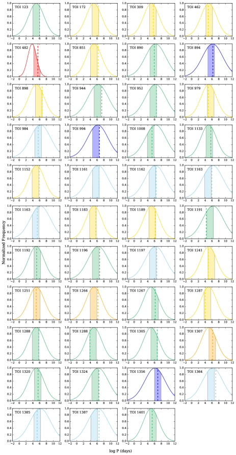
Figure 15: Expected binary period distributions for all TOIs with companions detected in 832nm based on the distribution presented in Raghavan et al. (2010). The shaded regions (color coded by spectral type of the primary as in Figure 6) show the orbital periods corresponding to projected separations at which speckle imaging at WIYN ($0.06-1.2"$) can detect companions. The dashed lines correspond to the separation of observed companions converted to $\log P$ space using the distance and mass of the primary star.

References

- Arenou et al. (2018) Arenou, F., Luri, X., Babusiaux, C., et al. 2018, A&A, 616, A17, doi: 10.1051/0004-6361/201833234
- Borucki et al. (2011) Borucki, W. J., Koch, D. G., Basri, G., et al. 2011, ApJ, 728, 117, doi: 10.1088/0004-637X/728/2/117
- Bouma et al. (2018) Bouma, L. G., Masuda, K., & Winn, J. N. 2018, AJ, 155, 244, doi: 10.3847/1538-3881/aabfb8
- Brown et al. (2011) Brown, T. M., Latham, D. W., Everett, M. E., & Esquerdo, G. A. 2011, AJ, 142, 112, doi: 10.1088/0004-6256/142/4/112
- Buchhave et al. (2011) Buchhave, L. A., Latham, D. W., Carter, J. A., et al. 2011, in AAS/Division for Extreme Solar Systems Abstracts, Vol. 2, AAS/Division for Extreme Solar Systems Abstracts, 19.17
- Ciardi et al. (2015) Ciardi, D. R., Beichman, C. A., Horch, E. P., & Howell, S. B. 2015, ApJ, 805, 16, doi: 10.1088/0004-637X/805/1/16
- Deacon et al. (2016) Deacon, N. R., Kraus, A. L., Mann, A. W., et al. 2016, MNRAS, 455, 4212, doi: 10.1093/mnras/stv2132
- Dupuy et al. (2016) Dupuy, T. J., Kratter, K. M., Kraus, A. L., et al. 2016, ApJ, 817, 80, doi: 10.3847/0004-637X/817/1/80
- Furlan & Howell (2020) Furlan, E., & Howell, S. B. 2020, ApJ, 898, 47, doi: 10.3847/1538-4357/ab9c9c
- Haghighipour (2006) Haghighipour, N. 2006, ApJ, 644, 543, doi: 10.1086/503351
- Horch et al. (2011) Horch, E. P., Gomez, S. C., Sherry, W. H., et al. 2011, AJ, 141, 45, doi: 10.1088/0004-6256/141/2/45
- Horch et al. (2014) Horch, E. P., Howell, S. B., Everett, M. E., & Ciardi, D. R. 2014, ApJ, 795, 60, doi: 10.1088/0004-637X/795/1/60
- Horch et al. (2009) Horch, E. P., Veillette, D. R., Baena Gallé, R., et al. 2009, AJ, 137, 5057, doi: 10.1088/0004-6256/137/6/5057
- Howell (2020) Howell, S. B. 2020, Frontiers in Astronomy and Space Sciences, 7, 10, doi: 10.3389/fspas.2020.00010
- Howell et al. (2011) Howell, S. B., Everett, M. E., Sherry, W., Horch, E., & Ciardi, D. R. 2011, AJ, 142, 19, doi: 10.1088/0004-6256/142/1/19
- Howell et al. (2019) Howell, S. B., Scott, N. J., Matson, R. A., Horch, E. P., & Stephens, A. 2019, AJ, 158, 113, doi: 10.3847/1538-3881/ab2f7b
- Howell et al. (2014) Howell, S. B., Sobeck, C., Haas, M., et al. 2014, PASP, 126, 398, doi: 10.1086/676406
- Jang-Condell (2015) Jang-Condell, H. 2015, ApJ, 799, 147, doi: 10.1088/0004-637X/799/2/147
- Kraus et al. (2016) Kraus, A. L., Ireland, M. J., Huber, D., Mann, A. W., & Dupuy, T. J. 2016, AJ, 152, 8, doi: 10.3847/0004-6256/152/1/8
- Lohmann et al. (1983) Lohmann, A. W., Weigelt, G., & Wirnitzer, B. 1983, Appl. Opt., 22, 4028, doi: 10.1364/AO.22.004028
- Matson et al. (2019) Matson, R. A., Howell, S. B., & Ciardi, D. R. 2019, AJ, 157, 211, doi: 10.3847/1538-3881/ab1755
- Matson et al. (2018) Matson, R. A., Howell, S. B., Horch, E. P., & Everett, M. E. 2018, AJ, 156, 31, doi: 10.3847/1538-3881/aac778
- Moe & Di Stefano (2017) Moe, M., & Di Stefano, R. 2017, ApJS, 230, 15, doi: 10.3847/1538-4365/aa6fb6
- Pecaut & Mamajek (2013) Pecaut, M. J., & Mamajek, E. E. 2013, ApJS, 208, 9, doi: 10.1088/0067-0049/208/1/9
- Rafikov & Silsbee (2015) Rafikov, R. R., & Silsbee, K. 2015, ApJ, 798, 69, doi: 10.1088/0004-637X/798/2/69
- Raghavan et al. (2010) Raghavan, D., McAlister, H. A., Henry, T. J., et al. 2010, ApJS, 190, 1, doi: 10.1088/0067-0049/190/1/1
- Ricker et al. (2015) Ricker, G. R., Winn, J. N., Vanderspek, R., et al. 2015, Journal of Astronomical Telescopes, Instruments, and Systems, 1, 014003, doi: 10.1117/1.JATIS.1.1.014003
- Scott et al. (2018) Scott, N. J., Howell, S. B., Horch, E. P., & Everett, M. E. 2018, PASP, 130, 054502, doi: 10.1088/1538-3873/aab484
- Stassun et al. (2018) Stassun, K. G., Oelkers, R. J., Pepper, J., et al. 2018, AJ, 156, 102, doi: 10.3847/1538-3881/aad050
- Sullivan et al. (2015) Sullivan, P. W., Winn, J. N., Berta-Thompson, Z. K., et al. 2015, ApJ, 809, 77, doi: 10.1088/0004-637X/809/1/77
- Teske et al. (2018) Teske, J. K., Ciardi, D. R., Howell, S. B., Hirsch, L. A., & Johnson, R. A. 2018, AJ, 156, 292, doi: 10.3847/1538-3881/aaed2d
- Thebault & Haghighipour (2015) Thebault, P., & Haghighipour, N. 2015, Planet Formation in Binaries, 309–340, doi: 10.1007/978-3-662-45052-9_13
- Ziegler et al. (2020) Ziegler, C., Tokovinin, A., Briceño, C., et al. 2020, AJ, 159, 19, doi: 10.3847/1538-3881/ab55e9
- Ziegler et al. (2018) Ziegler, C., Law, N. M., Baranec, C., et al. 2018, AJ, 156, 259, doi: 10.3847/1538-3881/aad80a