Characterization of a flux-driven Josephson parametric amplifier with near quantum-limited added noise for axion search experiments

Abstract

The axion, a hypothetical elementary pseudoscalar, is expected to solve the strong CP problem of QCD and is also a promising candidate for dark matter. The most sensitive axion search experiments operate at millikelvin temperatures and hence rely on instrumentation that carries signals from a system at cryogenic temperatures to room temperature instrumentation. One of the biggest limiting factors affecting the parameter scanning speed of these detectors is the noise added by the components in the signal detection chain. Since the first amplifier in the chain limits the minimum noise, low-noise amplification is of paramount importance. This paper reports on the operation of a flux-driven Josephson parametric amplifier (JPA) operating at around $2.3\text{\,}\mathrm{GHz}$ with added noise approaching the quantum limit. The JPA was employed as a first stage amplifier in an experimental setting similar to the ones used in haloscope axion detectors. By operating the JPA at a gain of $19\text{\,}\mathrm{dB}$ and cascading it with two cryogenic amplifiers operating at $4\text{\,}\mathrm{K}$, noise temperatures as low as $120\text{\,}\mathrm{mK}$ were achieved for the whole signal detection chain.

I Introduction

Axions are spin-0 particles that emerge as a result of the Peccei-Quinn mechanism which was originally proposed as a solution to the strong CP problem of quantum chromodynamics[1, 2]. They were also identified as viable candidates for all or a fraction of the cold dark matter in our universe[3, 4, 5]. It is possible to detect axions upon their conversion to microwave photons, using resonant cavities immersed in high magnetic fields[6]. Since the axion mass is unknown, these detectors employ a mechanism to scan different frequencies corresponding to different axion masses. The scanning rate of such detectors scales with $1/T_{\mathrm{sys}}^{2}$, where $T_{\mathrm{sys}}$ is the system noise background characterized in units of temperature. It can be decomposed as $T_{\mathrm{sys}}=T_{\mathrm{cav}}+T_{\mathrm{add}}$, where the first term denotes the noise temperature accompanying the signal itself and the second one denotes the noise added by the signal detection chain. Throughout this work, noise temperature refers to the added noise unless otherwise stated. In order to reduce $T_{\mathrm{cav}}$, the cavity is cooled to millikelvin temperatures. If the first amplifier has sufficiently high gain ($G_{1}$), its noise temperature ($T_{1}$) will be the dominant contribution to $T_{\mathrm{add}}$ as given by the well-known relation[7]: $T_{\mathrm{add}}=T_{1}+\frac{T_{\mathrm{rest}}}{G_{1}}$ where $T_{\mathrm{rest}}$ is the noise temperature of the whole chain except the first amplifier. Amplifiers based on Josephson junctions including microstrip superconducting quantum interference device amplifiers (MSA) and JPA have already been shown to be capable of gains higher than $30\text{\,}\mathrm{dB}$, and noise temperatures approaching the quantum limit[8, 9]. While an MSA has an internal shunt resistor used for biasing which hinders noise performance[10, 11], by design the JPA requires no resistive element to operate. Several experiments presently searching for dark matter axions have already adopted the JPA as the first amplifier[12, 13, 14]. In this work, the frequency coverage, gain and noise properties of a flux-driven JPA for use in an axion dark matter experiment operating around $2.3\text{\,}\mathrm{GHz}$ are investigated.

The power spectral density of the noise accompanying a signal measured in an impedance matched environment can be given as [15] :

$$S_{n}(f,T)=hf\left[\frac{1}{\exp{\left(\frac{hf}{k_{B}T}\right)}-1}+\frac{1}{2}\right]$$ (1)

where $h$ is Planck’s constant and $k_{B}$ is Boltzmann’s constant. The first term in the brackets is the mean number of quanta at frequency $f$ at the bath temperature $T$ and the second term is the contribution from zero-point fluctuations. The lower limit on noise temperature for linear phase-insensitive amplifiers is given by[16] $T_{Q}=\lim_{T\rightarrow 0}S_{n}(f,T)/(k_{B})=hf/(2k_{B})$ which is about $55.2\text{\,}\mathrm{mK}$ at $2.3\text{\,}\mathrm{GHz}$. Using a $2.3\text{\,}\mathrm{GHz}$ flux-driven JPA $T_{\mathrm{add}}\approx$120\text{\,}\mathrm{mK}$$ is achieved. This corresponds to a $T_{\mathrm{sys}}\approx$190\text{\,}\mathrm{mK}$$ for an axion haloscope experiment running at a bath temperature of $50\text{\,}\mathrm{mK}$. The lower bound for $T_{\mathrm{sys}}$ is given by the standard quantum limit[17] $T_{\mathrm{SQL}}=2T_{Q}$ which is about $110\text{\,}\mathrm{mK}$ at $2.3\text{\,}\mathrm{GHz}$.

II Flux-driven JPA

The equivalent circuit diagram of the tested device is shown in Figure 1. It consists of a superconducting quantum interference device (SQUID) attached to the end of a coplanar waveguide $\lambda/4$ resonator that is coupled via a capacitor ($C_{c}$) to the transmission line for the signal input and output. The SQUID acts as a variable inductor whose value depends on the magnetic flux passing through its loop. In the setup, a superconducting coil is used to provide the necessary DC flux ($\phi$) through the SQUID loop in order to tune the resonance frequency ($f_{r}$). Parametric amplification is achieved by modulating the flux through the SQUID using a pump signal. The pump tone is provided by a separate transmission line inductively coupled to the SQUID. The JPA is operated in the three-wave mixing mode[18] where the pump ($f_{p}$), the signal ($f_{s}$), and the idler ($f_{i}$) frequencies satisfy the relation $f_{p}=f_{s}+f_{i}$. The signal input and output share the same port. A circulator is used to separate them. Since the $\lambda/4$ resonator only allows odd harmonics, there is no measurable pump leakage to the output line. This prevents the stronger pump tone from saturating the rest of the amplifiers in the chain[19]. Figure 2 shows a schematic for the axion search experimental setup.

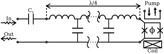
Figure 1: Equivalent circuit diagram of the JPA sample. The JPA was fabricated by photolithography of a Nb layer, deposited on a $0.3\text{\,}\mathrm{mm}$ thick Si substrate. The SQUID was placed on top of the Nb layer by E-beam lithography followed by shadow evaporation[20, 21]. The sample was attached to a printed circuit board (PCB) and the transmission lines were bonded with Al wires. The PCB was fixed onto a gold plated copper structure and placed inside a superconducting coil. The whole structure was covered tightly with a lead shield and attached to the mixing-chamber (MC) plate using a gold plated copper rod.

III Measurements

When there is no pump tone present, the JPA can be modeled as a resonator with a well-defined quality factor and resonance frequency which are functions of flux. The resonance frequency is estimated from the frequency domain phase response using a parameter fit[22]. The phase response is obtained by doing a transmission S-parameter measurement using a vector network analyzer (VNA) in the configuration as shown in Figure 2. The resonance frequency was measured as a function of the coil current (see Figure 3). It was found that the minimum observable resonance frequency was at $2.18\text{\,}\mathrm{GHz}$ and the maximum was $2.309\text{\,}\mathrm{GHz}$. The lower bound is due to the frequency band of the circulators which spans from $2.15\text{\,}\mathrm{GHz}$ to $2.60\text{\,}\mathrm{GHz}$. At the lower frequencies, the JPA becomes much more sensitive to flux noise due to a higher $\frac{\partial f_{r}}{\partial\phi}$. This work mainly focused on operation with frequencies above $2.2\text{\,}\mathrm{GHz}$.

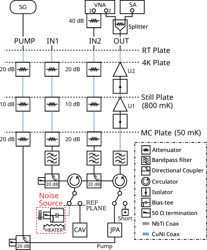
Figure 2: The experimental setup used in all the characterization measurements. SG, VNA, and SA stand for the signal generator, vector network analyzer, and spectrum analyzer, respectively. During this work, the switch that selects between the cavity and the noise source was always kept at the position shown in the figure. The ports IN2 and OUT were used to directly measure the JPA characteristics, bypassing the cavity. The microwave short element shown next to the JPA was used to bypass the JPA for calibration measurements. U1 and U2 are HEMT amplifiers with noise temperatures of $1.5\text{\,}\mathrm{K}$ and $5\text{\,}\mathrm{K}$, respectively.

During the experiments, the MC plate temperature was stabilized at $50\pm{}1\text{\,}\mathrm{mK}$. With the temperature fixed, the frequency response of the JPA is determined by three experimental variables: the coil current ($i_{b}$), the pump frequency ($f_{p}$), and the pump power ($P_{p}$). The measurements shown in this work had $i_{b}$ confined to the region where the flux through the SQUID loop is given by $-0.5\phi_{0}<\phi<0$, where $\phi_{0}$ is the magnetic flux quantum. Therefore, $f_{r}$ can be unambiguously converted to $\phi$ or $i_{b}$. All experiments began with a transmission measurement, with the resonance frequency tuned to $2.18\text{\,}\mathrm{GHz}$. This becomes the baseline measurement to be used for the duration of the experiment. When the result was compared to a separate measurement, in which a microwave short was put in place of the JPA, it was found that the baseline obtained via such an off-resonance measurement was at most $0.2\text{\,}\mathrm{dB}$ lossier than an ideal mirror. The JPA gain ($G_{J}$) was estimated by dividing the transmission magnitude response with the baseline’s magnitude response.

To investigate the gain behavior, a sweep over the parameters $i_{b}$, $f_{p}$, $P_{p}$ was made and the maximum gain was measured at each point. After each $i_{b}$ tuning step, the resonance frequency is estimated by performing a phase measurement and applying a parameter fit. With the detuning defined as $\delta=f_{p}/2-f_{r}$, the equigain contours had a minimum in necessary pump power around $\delta=0$, as shown in Figure 4(a). It was observed that for resonance frequencies above $2.299\text{\,}\mathrm{GHz}$ the minimum starts to shift to lower detunings which is attributed to pump-induced shifts in resonance frequency[22]. Figure 4(b) shows that the slice of $\delta=0$ can be used to achieve peak gains of up to $30\text{\,}\mathrm{dB}$ along the frequency range of the device.

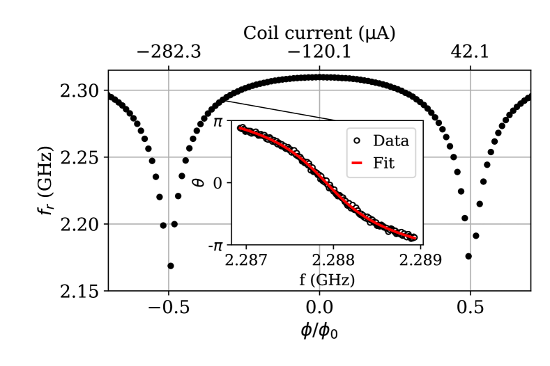
Figure 3: Resonance frequency versus flux obtained by sweeping the coil current and measuring the phase response at each step. One period corresponds to a current of $324.4\text{\,}\mathrm{\SIUnitSymbolMicro A}$. The inset shows the fit performed to estimate the resonance frequency for each applied flux.

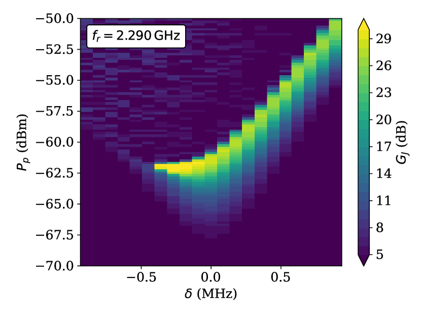
(a)

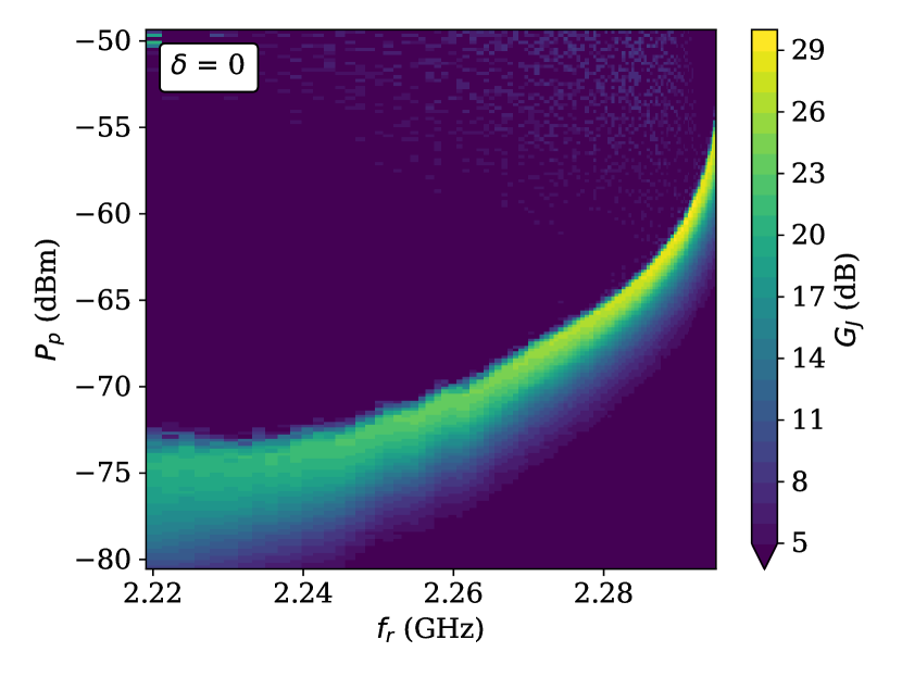
(b)

Figure 4: (a) Maximum gain measured as a function of detuning and pump power for a flux bias corresponding to $f_{r}=$2.29\text{\,}\mathrm{GHz}$$. (b) Maximum gain as a function of frequency and pump power with $f_{p}=2f_{r}$.

To investigate noise temperature, a methodology similar to the well-known Y-factor method[23] was used. A $50\text{\,}\mathrm{\SIUnitSymbolOhm}$ cryogenic microwave terminator was used as the noise source. A bias-tee was attached in front for improved thermalization of its inner conductor. These two components were fixed onto a gold-plated copper plate along with a ruthenium oxide temperature sensor and a $100\text{\,}\mathrm{\SIUnitSymbolOhm}$ resistor functioning as a heater. This plate was then fixed onto the MC plate so that the dominant thermalization was through a thin copper wire attached to the MC plate. The noise source was connected to the switch input using a superconducting coaxial cable, which provides thermal isolation while minimizing losses. Using a PID controller, the terminator temperature could be adjusted from $50\text{\,}\mathrm{mK}$ to $1\text{\,}\mathrm{K}$ without affecting the MC plate temperature. The noise power generated by the noise source was measured using a spectrum analyzer (SA) with $1\text{\,}\mathrm{kHz}$ resolution bandwidth after being amplified by the JPA and the rest of the signal detection chain. The power spectra were recorded at noise source temperatures ($T_{s}$) of $60120180\text{\,}\mathrm{mK}$. The power values were converted into power spectral densities (PSD) by dividing them with the noise bandwidth corresponding to the SA settings used. Before each PSD measurement, the JPA gain and passive resonance were measured. From these measurements, it was concluded that there were neither gain changes nor resonance shifts. From the obtained PSD values $S(T_{s})$, a fit was done to a function of the following form independently for each frequency bin (see  Figure 5) :

$$S(T_{s})=(2G_{J}-1)\frac{G_{L}G_{\mathrm{tot}}}{G_{J}}(S_{n}(T_{s})+rk_{B}T_{n}+\gamma)$$ (2)

where $S_{n}(T_{s})$ is the noise PSD of the source, $G_{\mathrm{tot}}$ is the total gain seen from the reference plane, $G_{L}$ is the loss factor between the $50\text{\,}\mathrm{\SIUnitSymbolOhm}$ terminator and the reference plane and $T_{n}$ is the noise temperature. The reference plane is at the end of the superconducting cable connected to the noise source (see Figure 2). Here, $r$ and $\gamma$ are factors that are explained in Appendix A.

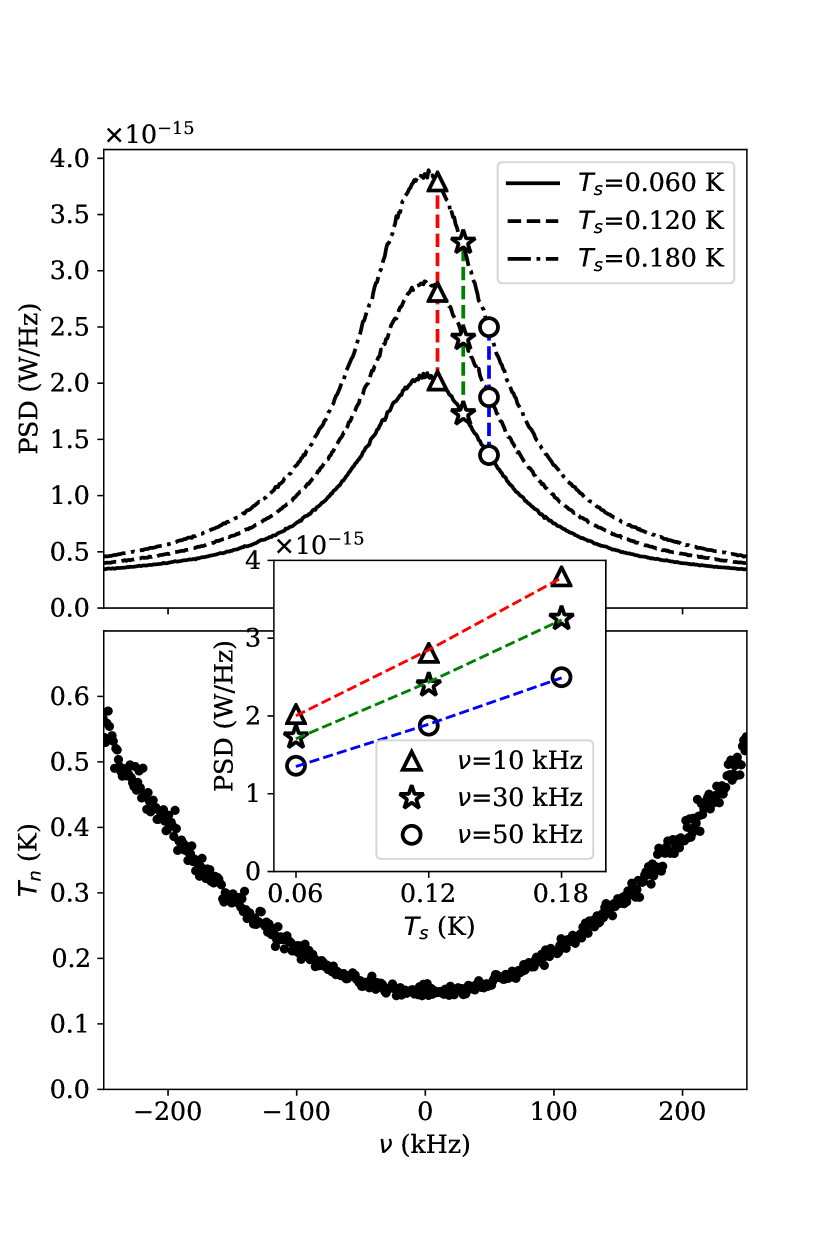
Figure 5: The upper plot shows the set of power spectra obtained during a noise temperature measurement performed for a tuning at $f_{r}=$2.305\text{\,}\mathrm{GHz}$$ with $f_{p}=2f_{r}$. The offset $\nu$ is defined as $\nu=f-f_{r}$ where $f$ is the center of the frequency bin at which the power was measured using the spectrum analyzer. $T_{s}$ is the temperature of the noise source. The inset shows three vertical slices which were fit with Equation 2. The lower plot shows the estimated noise temperature of the whole chain as a function of $\nu$.

Since the amplifier needs to be tuned along with the cavity during the axion experiment, the noise temperature was investigated at different frequencies. The measurements were done in $5\text{\,}\mathrm{MHz}$ steps from $2.282.305\text{\,}\mathrm{GHz}$. At each step, the pump power and resonance frequency were tuned such that the JPA gain was about $20$ $\mathrm{dB}$. From these measurements (Figure 6) a minimum noise temperature of $120\text{\,}\mathrm{mK}$ was observed at $2.28\text{\,}\mathrm{GHz}$.

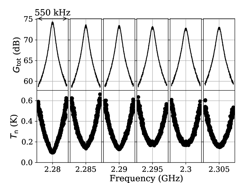
Figure 6: Total gain and the noise temperature of the whole chain for 6 tuning points with $19.3\pm{}0.5\text{\,}\mathrm{dB}$ JPA gain. Both quantities were estimated from noise temperature measurements. The small variations along tuning frequencies were mainly attributed to the losses due to the microwave components before the JPA.

Another important characteristic is the saturation that occurs when a narrowband signal is applied. For stable and predictable operation the JPA must be operated away from the effects of saturation. A common way to quantify the saturation of an amplifier is to determine the input power at which the gain is reduced by $1\text{\,}\mathrm{dB}$ ($P_{1\mathrm{dB}}$). The $P_{1\mathrm{dB}}$ was measured at $\delta=0$ for different frequencies and different pump powers corresponding to different gains. It is evident from the results (see Figure 7) that an axion-like signal with an expected power of $-180\text{\,}\mathrm{\milli}$ is far from saturating the device. While saturation from narrowband signals is avoidable to a certain extent, it was observed that thermal noise at the input can also saturate and alter the behavior of the device. For frequencies below $2.28\text{\,}\mathrm{GHz}$ with gains above $23\text{\,}\mathrm{dB}$, the device started showing saturated behavior with thermal noise when the noise source temperature was raised above $120\text{\,}\mathrm{mK}$, which was done to measure noise temperature. While this does not necessarily mean that the device is unusable below these frequencies, it renders the direct measurement of the noise temperature using a noise source unreliable for these frequency and gain regions.

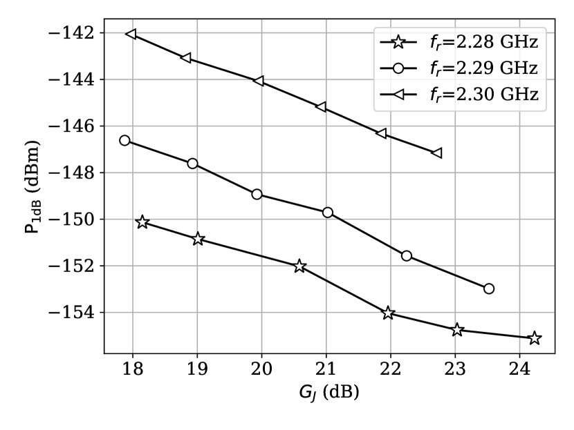
Figure 7: Saturation measurements for three different $f_{r}$. Each measurement was done by sweeping the signal powers from the VNA and observing at which input power the gain reduces by 1 dB. The horizontal axis corresponds to the unsaturated gain measured with the lowest signal power available from VNA.

IV Conclusion

In conclusion, a flux-driven JPA, tunable in the range $2.22.305\text{\,}\mathrm{GHz}$ was demonstrated and determined to be operational for use in axion search experiments. The added noise temperatures of the receiver chain were measured using a noise source at a location as close as possible to the origin of the axion signal. With an added noise temperature of $120\text{\,}\mathrm{mK}$ the system was shown to reach $T_{\mathrm{sys}}\approx 1.7T_{\mathrm{SQL}}$. This is the first record of $T_{\mathrm{sys}}$ below $2T_{\mathrm{SQL}}$ for an axion haloscope setup operating below $10\text{\,}\mathrm{GHz}$. The saturation input power for the JPA was observed to be more than adequate for an axion-like signal. Currently, the tested JPA is being used as part of a KSVZ[24, 25] sensitive axion search experiment at the Center for Axion and Precision Physics Research (CAPP). The system is taking physics data with a scanning speed that has been improved more than an order of magnitude. We expect that further optimization of the JPA design could result in improved instantaneous bandwidth and tuning range.

This work was supported by the Institute for Basic Science (IBS-R017–D1–2021–a00) and JST ERATO (Grant No. JPMJER1601). A. F. van Loo is supported by a JSPS postdoctoral fellowship.

Appendix A Noise Temperature Estimation

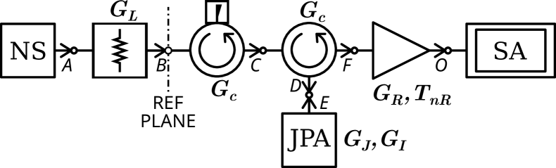
Figure 8: The simplified model used for the noise temperature estimations conducted in this work. Bold letters denote the power gains of components. The reference plane marks the input of the detector chain. Arrows denote the flow of power entering the nodes shown with a small circle. $G_{L}$ is a composite gain factor for everything between the noise source and the reference plane. $G_{c}$ is the circulator gain factor. $G_{J}$ is the signal and $G_{I}$ is the idler gain for the JPA. The amplifier gain $G_{R}$ and noise temperature $T_{nR}$ contain the effects of all elements after the last circulator, including SA noise. For simplicity, circulators are assumed to have complete rotational symmetry with respect to their ports and to be completely identical to each other.

The output PSD from a component with its input connected to a matched source can be written as :

$$S_{\mathrm{O}}=GS_{\mathrm{in}}+S_{\mathrm{added}}$$ (3)

where $S_{\mathrm{in}}$ is the source PSD, $G$ is the power gain of the component, and $S_{\mathrm{added}}$ is the noise added by it. The noise temperature ($T_{n}$) is a measure of the added noise at the output of a component. By convention, it is defined as if it is for noise entering the device itself: $T_{n}=S_{\mathrm{added}}/(k_{B}G)$. The entire detection chain (see Figure 8), from the reference plane to the spectrum analyzer, can be described as a single composite component with $G=G_{\mathrm{tot}}$ and noise temperature $T_{n}$.

The noise temperature can be defined for a situation similar to the experimental one where a narrowband axion signal with power $A$ is present. This signal enters the chain from a source connected to the reference plane. Assuming the source is thermalized to the MC plate with the temperature $T_{f}$, then the defining relation for $T_{n}$ can be written as :

$$S_{O}=G_{\mathrm{tot}}(\underbrace{A\delta(f-f_{s})+S_{n}(T_{f})}_{S_{\mathrm{in}}}+k_{B}T_{n})$$ (4)

where $S_{O}$ is the PSD at the output, $G_{\mathrm{tot}}$ is the total power gain for the signal from the reference plane, $S_{n}$ is the noise coming from the source itself. The main idea here is that if one has a reliable estimate of $T_{n}$, and understands the source environment well ($S_{n}(T_{f})$), it is straightforward to estimate $A$ without the precise knowledge of $G_{\mathrm{tot}}$. This is possible since $S_{O}$ can be easily measured at two frequencies $f_{s}$ and $f_{s}^{\prime}$ using a spectrum analyzer. Provided that $|f_{s}-f_{s}^{\prime}|$ is small enough so that $T_{n}$ is approximately the same for both frequencies, $A$ can be estimated from these two measurements. This approach forms the basis of the analysis methods applied in axion dark matter search experiments[26, 27, 28, 29].

The detection chain consists of passive components, the JPA and the HEMT amplifiers. Each one of these adds noise in a different way. A passive component at physical temperature $T_{f}$ has $S_{\mathrm{added}}=(1-G)S_{n}(T_{f})$. The HEMT amplifier noise is usually estimated from measurements. The JPA adds noise by two main mechanisms. The first one is by amplifying the input noise at the idler mode onto the signal mode. The second one is via the losses or other dissipation mechanisms inside or before the sample. Ideally, the latter can be made zero, whereas the former will approach to the half-photon added noise in the limit of a $0\text{\,}\mathrm{K}$ bath temperature.

Using the model shown in Figure 8, it is straightforward to write a relation for the output PSD. For clarity, the explicit frequency dependence of the thermal noise $S_{n}$ and of the gains will be omitted. Also, the approximation $S_{n}(f,T)\approx S_{n}(f_{p}-f,T)$ will be denoted with the shorthand $S_{nf}=S_{n}(f,T_{f})$. This approximation has less than 30 ppm error given that $|2f-f_{p}|<$100\text{\,}\mathrm{kHz}$$. Note that $100\text{\,}\mathrm{kHz}$ is the typical bandwidth for the JPA tested in this work. Furthermore, the transmission characteristics of the microwave components will be assumed to not vary on a scale of $100\text{\,}\mathrm{kHz}$. Using the gain symbols for components as shown in Figure 8, the power flow at each node in terms of their PSD is written as :

$$\begin{split}S_{B}&=G_{L}S_{A}+(1-G_{L})S_{nf}\\ S_{C}&=G_{c}S_{B}+(1-G_{c})S_{nf}\\ S_{D}&=G_{c}S_{C}+(1-G_{c})S_{nf}\\ S_{E}&=G_{J}S_{D}+G_{I}S_{D}+G_{J}S_{j}\\ S_{F}&=G_{c}S_{E}+(1-G_{c})S_{nf}\\ S_{O}&=G_{R}(S_{F}+k_{B}T_{nR})\end{split}$$ (5)

The idler gain is denoted by $G_{I}$, and is substituted using $G_{I}=G_{J}-1$[30] in the following derivations. As shown in Equation 5, the idler contribution to the noise appears as $G_{I}S_{D}$. The symbol $S_{j}$ denotes an unknown noise density added at the JPA stage which does not contribute to the quantum limit but rather contains losses or other mechanisms of stationary noise. Note that the noise propagating back from the later stages is also included in $S_{j}$. The output $S_{O}$ can be written for two cases. In the first case, the noise source is operational at temperature $T_{s}$, and in the second case, a signal source at temperature $T_{f}$ is connected to the reference plane. The former case describes the measurement situation, whereas the latter case is only used to define $T_{n}$ in terms of the parameters in the model. For the first case, i.e.  $S_{A}=S_{n}(T_{s})$, the output PSD can be written as :

$$S_{O}^{(1)} =\underbrace{G_{R}G_{c}^{3}G_{L}(2G_{J}-1)}_{G_{\mathrm{noise}}}\left[S_{n}(T_{s})+S_{\alpha}\right]$$ (6)

$$S_{\alpha} =\lambda^{(1)}S_{nf}+\frac{G_{J}S_{j}}{(2G_{J}-1)G_{c}^{2}G_{L}}+\left.\frac{k_{B}T_{nR}}{G_{c}^{3}G_{L}(2G_{J}-1)}\right.$$ (7)

$$\lambda^{(1)} =\beta_{l}+\frac{\beta_{c}}{G_{L}}+\frac{\beta_{c}}{G_{c}G_{L}}+\frac{\beta_{c}}{G_{c}^{2}G_{L}}$$ (8)

$$\beta_{\mathord{\color[rgb]{0,0,0}\bullet}} \equiv\frac{1}{G_{\mathord{\color[rgb]{0,0,0}\bullet}}}-1$$ (9)

The output for the second case, where $S_{B}=A\delta(f-f_{s})+S_{nf}$, is written as :

$$S_{O}^{(2)} =\underbrace{G_{J}G_{c}^{3}G_{R}}_{G_{\mathrm{tot}}}\left[S_{B}+k_{B}T_{n}\right]$$ (10)

$$k_{B}T_{n} =\lambda^{(2)}S_{nf}+\frac{S_{j}}{G_{c}^{2}}+k_{B}\frac{T_{nR}}{G_{c}^{3}G_{J}}$$ (11)

$$\lambda^{(2)} =\left[\frac{G_{J}-1}{G_{J}}+\left(\beta_{c}+\frac{\beta_{c}}{G_{c}}\right)\frac{2G_{J}-1}{G_{J}}+\frac{\beta_{c}}{G_{c}^{2}}\right]$$ (12)

Here, the unknowns are $S_{j}$, $T_{nR}$ and $G_{R}$. It is clear from Equations 11 and 12 that $T_{n}$ approaches $T_{Q}$ as expected in the limits of $G_{J}\gg 1$, $G_{c}\rightarrow 0$, and $G_{L}\rightarrow 0$. Using Equations 6, 7 and 11 $,S_{O}^{(1)}$ can be rewritten as :

$$\begin{split}S_{O}^{(1)}&=\frac{G_{\mathrm{tot}}}{r}(S_{n}(T_{s})+rk_{B}T_{n}+\gamma)\\ r&=\frac{G_{J}}{G_{L}(2G_{J}-1)}\\ \gamma&=\left(\lambda^{(1)}-r\lambda^{(2)}\right)S_{nf}\end{split}$$ (13)

This relation is used to perform a fit with $G_{\mathrm{tot}}$ and $T_{n}$ as the fit parameters. For the estimations, the parameters $G_{L}$ and $G_{c}$ were taken as $-0.05\text{\,}\mathrm{dB}$, and $-0.4\text{\,}\mathrm{dB}$ respectively. Some typical values for $r$ and $\gamma/k_{B}$ can be found in Table 1.

Table 1: Calculated $r$ and $\gamma/k_{B}$ for typical component losses and $T_{f}=$50\text{\,}\mathrm{mK}$$.

$G_{J}($\mathrm{dB}$)$	$G_{L}($\mathrm{dB}$)$	$G_{c}($\mathrm{dB}$)$	$r$	$\gamma/k_{B}($\mathrm{mK}$)$
15	0	-0.3	0.508	-31.1
15	-0.2	-0.5	0.532	-26.8
20	0	-0.3	0.503	-31.4
20	-0.2	-0.5	0.526	-27.1
19	-0.05	-0.4	0.509	-29.8

References

- Peccei and Quinn [1977] R. D. Peccei and H. R. Quinn, Phys. Rev. Lett. 38, 1440 (1977).
- Weinberg [1978] S. Weinberg, Phys. Rev. Lett. 40, 223 (1978).
- Preskill, Wise, and Wilczek [1983] J. Preskill, M. B. Wise, and F. Wilczek, Phys. Lett. B 120, 127 (1983).
- Dine and Fischler [1983] M. Dine and W. Fischler, Phys. Lett. B 120, 137 (1983).
- Abbott and Sikivie [1983] L. F. Abbott and P. Sikivie, Phys. Lett. B 120, 133 (1983).
- Sikivie [1983] P. Sikivie, Phys. Rev. Lett. 51, 1415 (1983).
- Friis [1944] H. Friis, Proceedings of the IRE 32, 419 (1944).
- Castellanos-Beltran and Lehnert [2007] M. A. Castellanos-Beltran and K. W. Lehnert, Appl. Phys. Lett. 91 (2007), 10.1063/1.2773988.
- Kinion and Clarke [2011] D. Kinion and J. Clarke, Appl. Phys. Lett. 98, 10 (2011).
- Uchaikin et al. [2019] S. Uchaikin, A. Matlashov, D. Lee, W. Chung, S. J. Oh, Y. Semertzidis, V. Zakosarenko, Ç Kutlu, A. van Loo, Y. Urade, S. Kono, M. Schmelz, R. Stolz, and Y. Nakamura, in 2019 IEEE International Superconductive Electronics Conference (ISEC) (2019) pp. 1–3.
- André et al. [1999] M. O. André, M. Mück, J. Clarke, J. Gail, and C. Heiden, Appl. Phys. Lett. 75, 698 (1999).
- Braine et al. [2020] T. Braine, R. Cervantes, N. Crisosto, N. Du, S. Kimes, L. J. Rosenberg, G. Rybka, J. Yang, D. Bowring, A. S. Chou, R. Khatiwada, A. Sonnenschein, W. Wester, G. Carosi, N. Woollett, L. D. Duffy, R. Bradley, C. Boutan, M. Jones, B. H. Laroque, N. S. Oblath, M. S. Taubman, J. Clarke, A. Dove, A. Eddins, S. R. O’kelley, S. Nawaz, I. Siddiqi, N. Stevenson, A. Agrawal, A. V. Dixit, J. R. Gleason, S. Jois, P. Sikivie, J. A. Solomon, N. S. Sullivan, D. B. Tanner, E. Lentz, E. J. Daw, J. H. Buckley, P. M. Harrington, E. A. Henriksen, and K. W. Murch, Phys. Rev. Lett. 124, 101303 (2020).
- Brubaker et al. [2017a] B. M. Brubaker, L. Zhong, Y. V. Gurevich, S. B. Cahn, S. K. Lamoreaux, M. Simanovskaia, J. R. Root, S. M. Lewis, S. Al Kenany, K. M. Backes, I. Urdinaran, N. M. Rapidis, T. M. Shokair, K. A. van Bibber, D. A. Palken, M. Malnou, W. F. Kindel, M. A. Anil, K. W. Lehnert, and G. Carosi, Phys. Rev. Lett. 118, 061302 (2017a).
- Crescini et al. [2020] N. Crescini, D. Alesini, C. Braggio, G. Carugno, D. D’Agostino, D. Di Gioacchino, P. Falferi, U. Gambardella, C. Gatti, G. Iannone, C. Ligi, A. Lombardi, A. Ortolan, R. Pengo, G. Ruoso, and L. Taffarello, Phys. Rev. Lett. 124, 171801 (2020).
- Callen and Welton [1951] H. B. Callen and T. A. Welton, Phys. Rev. 83, 34 (1951).
- Clerk et al. [2010] A. A. Clerk, M. H. Devoret, S. M. Girvin, F. Marquardt, and R. J. Schoelkopf, Rev. Mod. Phys. 82, 1155 (2010).
- Caves [1982] C. M. Caves, Phys. Rev. D 26, 1817 (1982).
- Roy and Devoret [2016] A. Roy and M. Devoret, Comptes Rendus Physique 17, 740 (2016), quantum microwaves / Micro-ondes quantiques.
- Yamamoto et al. [2008] T. Yamamoto, K. Inomata, M. Watanabe, K. Matsuba, T. Miyazaki, W. D. Oliver, Y. Nakamura, and J. S. Tsai, Appl. Phys. Lett. 93, 042510 (2008).
- Dolan [1977] G. J. Dolan, Appl. Phys. Lett. 31, 337 (1977).
- Zhong et al. [2013] L. Zhong, E. P. Menzel, R. Di Candia, P. Eder, M. Ihmig, A. Baust, M. Haeberlein, E. Hoffmann, K. Inomata, T. Yamamoto, Y. Nakamura, E. Solano, F. Deppe, A. Marx, and R. Gross, New Journal of Physics 15 (2013), 10.1088/1367-2630/15/12/125013.
- Krantz et al. [2013] P. Krantz, Y. Reshitnyk, W. Wustmann, J. Bylander, S. Gustavsson, W. D. Oliver, T. Duty, V. Shumeiko, and P. Delsing, New Journal of Physics 15, 105002 (2013).
- Engen [1970] G. F. Engen, IEEE Transactions on Instrumentation and Measurement 19, 344 (1970).
- Kim [1979] J. E. Kim, Phys. Rev. Lett. 43, 103 (1979).
- Shifman, Vainshtein, and Zakharov [1980] M. A. Shifman, A. I. Vainshtein, and V. I. Zakharov, Nuclear Physics, Section B 166, 493 (1980).
- Lee et al. [2020] S. Lee, S. Ahn, J. Choi, B. R. Ko, and Y. K. Semertzidis, Phys. Rev. Lett. 124, 101802 (2020).
- Jeong et al. [2020] J. Jeong, S. Youn, S. Bae, J. Kim, T. Seong, J. E. Kim, and Y. K. Semertzidis, Phys. Rev. Lett. 125, 221302 (2020).
- Asztalos et al. [2001] S. Asztalos, E. Daw, H. Peng, L. J. Rosenberg, C. Hagmann, D. Kinion, W. Stoeffl, K. van Bibber, P. Sikivie, N. S. Sullivan, D. B. Tanner, F. Nezrick, M. S. Turner, D. M. Moltz, J. Powell, M.-O. André, J. Clarke, M. Mück, and R. F. Bradley, Phys. Rev. D 64, 092003 (2001).
- Brubaker et al. [2017b] B. M. Brubaker, L. Zhong, S. K. Lamoreaux, K. W. Lehnert, and K. A. van Bibber, Phys. Rev. D 96, 123008 (2017b).
- Yurke et al. [1989] B. Yurke, L. R. Corruccini, P. G. Kaminsky, L. W. Rupp, A. D. Smith, A. H. Silver, R. W. Simon, and E. A. Whittaker, Phys. Rev. A 39, 2519 (1989).