ALMA Observations of Massive Clouds in the Central Molecular Zone: Ubiquitous Protostellar Outflows

Abstract

We observe 1.3 mm spectral lines at 2000 AU resolution toward four massive molecular clouds in the Central Molecular Zone of the Galaxy to investigate their star formation activities. We focus on several potential shock tracers that are usually abundant in protostellar outflows, including SiO, SO, CH₃OH, H₂CO, HC₃N, and HNCO. We identify 43 protostellar outflows, including 37 highly likely ones and 6 candidates. The outflows are found toward both known high-mass star forming cores and less massive, seemingly quiescent cores, while 791 out of the 834 cores identified based on the continuum do not have detected outflows. The outflow masses range from less than 1 $M_{\odot}$ to a few tens of $M_{\odot}$, with typical uncertainties of a factor of 70. We do not find evidence of disagreement between relative molecular abundances in these outflows and in nearby analogs such as the well-studied L1157 and NGC7538S outflows. The results suggest that i) protostellar accretion disks driving outflows ubiquitously exist in the CMZ environment, ii) the large fraction of candidate starless cores is expected if these clouds are at very early evolutionary phases, with a caveat on the potential incompleteness of the outflows, iii) high-mass and low-mass star formation is ongoing simultaneously in these clouds, and iv) current data do not show evidence of difference between the shock chemistry in the outflows that determines the molecular abundances in the CMZ environment and in nearby clouds.

1 INTRODUCTION

Star formation in the Central Molecular Zone (CMZ; the inner 500 pc of our Galaxy) has been a controversial topic. With more than $10^{7}$ $M_{\odot}$ gas of mean density at $10^{4}$ cm^-3 (Morris & Serabyn, 1996; Ferrière et al., 2007; Longmore et al., 2013a), the CMZ exhibits about 10 times less efficient star formation than expected by dense gas-star formation relations that have been tested toward nearby molecular clouds and external galaxies (Longmore et al., 2013a; Kruijssen et al., 2014; Barnes et al., 2017). Massive clouds in the CMZ have been suggested to be progenitors of young massive star clusters (Longmore et al., 2013b; Rathborne et al., 2015; Walker et al., 2016), but observations reveal inefficient star formation in these clouds (Kauffmann et al., 2017; Walker et al., 2018; Lu et al., 2019a, b), with an overall dearth of compact dense cores across much of the CMZ (Battersby et al., 2020; Hatchfield et al., 2020).

In Lu et al. (2020, hereafter Paper I), we reported ALMA Band 6 continuum observations toward four clouds, including the 20 km s^-1 cloud, the 50 km s^-1 cloud, Sgr B1-off, and Sgr C, which are some of the most massive clouds in the CMZ and show signs of embedded star formation (Kauffmann et al., 2017). We identified hundreds of 2000 AU-scale cores in three of the clouds (the exception being the 50 km s^-1 cloud), and suggested that the three clouds will likely form OB associations that contain less than 20 high-mass stars and have a spatial extent of $\sim$5–10 pc. In the 50 km s^-1 cloud, no cores above the 5$\sigma$ level and larger than the synthesized beam were found, likely because this cloud has evolved to a much later phase when cold cores vanish and H ii regions dominate (Mills et al., 2011). At sub-0.1 pc scales, we found evidence of thermal Jeans fragmentation and a similar core mass function as in Galactic disk clouds, which may hint at similar star formation processes at small spatial scales taking place in the CMZ and elsewhere in the Galaxy.

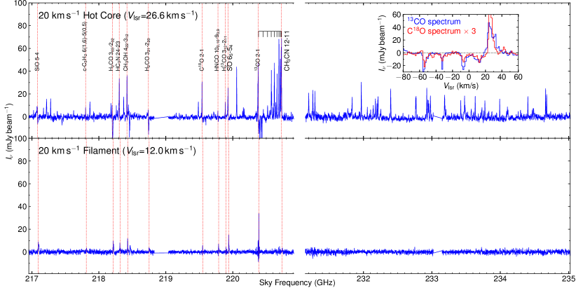
Figure 1: Typical 1.3 mm spectra captured by ALMA, toward a star forming hot core and a chemically quiescent region spatially offset from star forming regions in the 20 km s^-1 cloud, respectively. The corresponding positions where the spectra are extracted are denoted by blue arrows and labeled in Figure 2. The lines plotted in Figure 2 are highlighted by vertical dashed lines. Most of the other lines detected toward the hot core are from rotational transitions of complex organic molecules. The inset shows the ¹³CO and C¹⁸O spectra toward the hot core along the $V_{\text{lsr}}$ axis. Absorption at $-$55, $-$30, and $-$5 km s^-1 owing to foreground gas is seen.

However, it is unclear whether these cores are prestellar or protostellar (i.e., whether there are already embedded protostars). In Lu et al. (2019a, b), we used H₂O masers, class II CH₃OH masers, and ultra-compact H ii regions to trace high-mass star formation and identified a few high-mass star forming regions in these clouds. Yet, the relatively poor resolution of those observations, $\sim$4″ ($\sim$33,000 AU), prevents us from associating a particular high-mass star formation tracer with any of the 2000 AU-scale cores in Paper I. Further, the ultra-compact H ii regions trace a later evolutionary phase of high-mass star formation, such that we may miss low to intermediate-mass star formation or early evolutionary phases of high-mass star formation. The masers are able to reveal low to intermediate-mass star formation, but suffer from potentially low detection rates and contamination from masing sources other than star forming regions.

To this end, molecular outflows associated with the 2000 AU-scale cores are a promising tracer of star formation. Outflows are ubiquitously found in star forming regions, and are detected around both low-mass and high-mass protostars across a wide range of evolutionary phases as long as gas accretion is underway (e.g., Zhang et al., 2005; Arce et al., 2010; Li et al., 2019, 2020). Several molecular lines that are potential outflow tracers were observed along with the continuum data in Paper I. Therefore, in this paper we use the lines to search for direct evidence of star formation in the form of protostellar outflows.

In addition, the shock chemistry in protostellar outflows in the CMZ is poorly constrained. For one thing, only a handful of protostellar outflows have been detected in the CMZ, which are mostly in the most actively star forming region, Sgr B2 (Qin et al., 2008; Higuchi et al., 2015). More recently, with the advent of high resolution ALMA observations, more outflows are being detected outside of Sgr B2 (e.g., D. Walker et al. submitted, 2020). On the other hand, the chemistry of the molecular gas at pc scales in the CMZ seems to be distinct from that in the solar neighborhood, with noticeable enhancement of complex organic molecules and shock tracers throughout the CMZ (Martín-Pintado et al., 1997; Requena-Torres et al., 2006, 2008; Menten et al., 2009), likely caused by the extreme conditions such as widespread shocks, high gas temperatures, high cosmic ray fluxes, and high X-ray fluxes (Mills & Morris, 2013; Ginsburg et al., 2016; Henshaw et al., 2016; Padovani et al., 2020; Bykov et al., 2020). Once we obtain a large sample of outflows, we will be able to systematically compare the relative abundances of the molecules in these outflows to those in nearby clouds, to investigate whether the shock chemistry differs between the CMZ and elsewhere in the Galaxy at sub-0.1 pc scales.

In the following, we first introduce our ALMA observation and data reduction strategies, as well as an assessment of the missing flux issue in Section 2. Then in Section 3 we summarize our observational results, including an overview of the line emission and a visual identification of outflows. In Section 4, we estimate column densities, molecular abundances, and masses of the outflows, and discuss the implications to chemistry and star formation. We conclude our paper in Section 5. In Appendix A, we introduce the procedures to estimate column densities using the molecular line data. In Appendix B, we list properties of the identified outflows in a detailed table. Throughout the paper we adopt a distance of 8.178 kpc to the CMZ (Gravity Collaboration et al., 2018).

2 OBSERVATIONS AND DATA REDUCTION

2.1 ALMA Observations

The ALMA observations were carried out in the C40-3 and C40-5 configurations in April and July of 2017 (project code: 2016.1.00243.S). Details of the sample selection, observation setup, and data calibration can be found in Paper I. The four clouds in the sample are listed in Table 1. The covered fields are chosen based on Submillimeter Array (SMA) and VLA observations that revealed potential sites of high-mass star formation including H₂O masers and massive dense cores of 0.2 pc scale (Lu et al., 2019a). We imaged the Band 6 (1.3 mm) spectral lines using CASA 5.4.0. The covered frequencies range from 217–221 GHz to 231–235 GHz with a uniform channel width of 0.977 MHz (1.3 km s^-1). The effective spectral resolution is 1.129 MHz (1.5 km s^-1) after a Hanning smoothing done by the observatory.

We first manually identified line-free channels in the visibility data, and fed them to the uvcontsub task to subtract the continuum baseline. Then we used the tclean task to image the spectral lines, with Briggs weighting and a robust parameter of 0.5, and multi-scale algorithm with scales of [0, 5, 15, 50, 150] pixels and a pixel size of 0$\farcs$04. The image reconstruction was carried out in a two-step manner: first, the auto-masking algorithm with the recommended parameters was employed in tclean to automatically identify and clean signals; then the tclean task was restarted using clean models and residuals from the previous step as input, and all pixels within 20% primary beam response included in the clean mask, to a threshold of $\sim$5$\sigma$ (8 mJy beam^-1 per channel), in order to clean any residual significant signals. In a few cases where strong spatially diffuse emission is detected (e.g., H₂CO in the 20 km s^-1 cloud), a threshold of 8 mJy beam^-1 may be too low and causes the clean algorithm to diverge. We elevated the threshold to 10 mJy beam^-1 for these lines. We have compared images produced by our automatic approach with those produced by a fine-tuned manual tclean of several lines, and found that the images are almost identical.

The resulting synthesized beam is on average 0$\farcs$28$\times$0$\farcs$19 (equivalent to 2200 AU$\times$1500 AU) but slightly varies between lines. The largest recoverable angular scale is 10″ ($\sim$0.4 pc) with a shortest baseline length of 17 m. The achieved spectral line rms is between 1.6–2.0 mJy beam^-1 (0.8–1.0 K in brightness temperatures) per 1.3 km s^-1 channel depending on frequencies and regions.

Table 1: Properties of the clouds.

Cloud	$V_{\text{lsr}}$	No. of cores	No. of outflows	Fraction with outflows	$\bar{X}$(SiO)	$\bar{X}$(SO)	$\bar{X}$(CH3OH)	$\bar{X}$(H2CO)	$\bar{X}$(HC3N)	$\bar{X}$(HNCO)
(1)	(2)	(3)	(4)	(5)	(6)	(7)	(8)	(9)	(10)	(11)
The 20 km s-1 cloud	12.5	471	20	0.042	1.69$\times$10-9	7.10$\times$10-9	0.99$\times$10-7	0.80$\times$10-8	0.65$\times$10-9	4.40$\times$10-9
Sgr B1-off	31.1	89	5	0.056	1.39$\times$10-9	6.19$\times$10-9	0.86$\times$10-7	1.09$\times$10-8	1.24$\times$10-9	4.32$\times$10-9
Sgr C	$-$52.6	274	18	0.066	2.39$\times$10-9	9.87$\times$10-9	1.33$\times$10-7	1.84$\times$10-8	1.48$\times$10-9	5.44$\times$10-9
All three clouds	$\cdots$	834	43	0.052	2.05$\times$10-9	8.49$\times$10-9	1.15$\times$10-7	1.40$\times$10-8	1.16$\times$10-9	4.95$\times$10-9
The 50 km s-1 cloud	48.6	0	0	$\cdots$	$\cdots$	$\cdots$	$\cdots$	$\cdots$	$\cdots$	$\cdots$

Note. — Column (1): cloud name. Column (2): $V_{\text{lsr}}$ of the cloud (Kauffmann et al., 2017). Column (3): number of the identified cores (Paper I). Column (4): number of the identified outflows in this work. Column (5): fraction of the cores that have identified outflows. Columns (6–11): mean molecular abundances of all the outflows in the cloud. Only the abundances with independent measurements are considered (entries without notes in the last column in Table 3; see Section 4.1.2).

2.2 Assessing the Missing Flux

By their nature, interferometric observations do not recover structures on size scales larger than their largest recoverable angular scale (10″ or 0.4 pc for these observations). If structures larger than this exist in the field, the flux captured by interferometers will be smaller than the true flux, which is referred to as the missing flux problem. Spatially extended ($\gtrsim$0.4 pc) structures including outflows and filaments are seen in the spectral line images. In principle, we can combine our data with shorter baseline as well as single-dish data to recover any spatially extended emission. Such data are available from the SMA and the Caltech Submillimeter Observatory (CSO) observations published in Lu et al. (2017, 2019a) and Battersby et al. (2020).

However, we note several issues that prevent us from efficiently combining the data: i) The sensitivity of the SMA data is not optimal for the combination. For several regions, e.g., Sgr C, the SMA observation recovers an even smaller flux than the ALMA data, suggesting that some weaker emission is missed by the SMA data due to its lower sensitivity. ii) Several regions of particular interest (e.g., the western part of Sgr C) are not well sampled by existing SMA observations.

We attempted to combine the ALMA and SMA data, by concatenating the visibility data and imaging them together. The resulting image is not improved compared to the ALMA image, e.g., the rms becomes higher, and the integrated fluxes of several spatially extended structures do not increase significantly (in the extreme case of Sgr C, the fluxes even decrease).

Therefore, we conclude that the imaging of diffuse structures does not benefit from the addition of the SMA data. This does not rule out the possibility that better shorter baseline data may help. A longer SMA observation, or an ACA observation that provides better sensitivity than the SMA, would be necessary to be combined with the ALMA data to recover spatially extended emission.

Meanwhile, we compared the integrated fluxes recovered by the CSO and ALMA, focusing on the SiO emission in Sgr C which is the most spatially extended in our data and thus the most affected by the missing flux. In a circle of 50″ diameter centered in between the two clusters in Sgr C, the ALMA/CSO SiO integrated fluxes are measured to be 120/200 Jy km s^-1. The ALMA data recover 60% of the flux observed by the CSO. We thus estimate an upper limit of 40% for the missed flux in our ALMA data. In Section 4.1.4, we will see that this does not affect our estimate of outflow properties, as the dominant uncertainty is the molecular abundance that is unconstrained by several orders of magnitude.

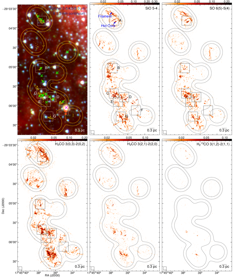
Figure 2: Molecular line emission in the 20 km s^-1 cloud. The inner and outer dashed loops in all panels demonstrate the 50% and 30% primary beam responses of the ALMA mosaics. The first panel shows a three-color image made from Spitzer IRAC 3.6, 4.5, and 5.8 µm bands, with yellow contours overlaid illustrating the ALMA 1.3 mm continuum emission at levels of [5,25,45]$\times$40 $\mu$Jy beam^-1. Positions of H₂O masers are marked by crosses, among which those with AGB star counterparts (Lu et al., 2019a) are colored in magenta. The other panels show integrated intensities of molecular lines in a logarithmic scale, which are integrated in a velocity range of [$-20$,$40$] km s^-1, except for CH₃OH and CH₃CN where this range is adjusted to avoid confusion with adjacent lines. The colorbars are in unit of Jy beam^-1 km s^-1. In selected panels, black boxes show regions where outflows are identified, with zoomed-in views presented in Figures 6–22.

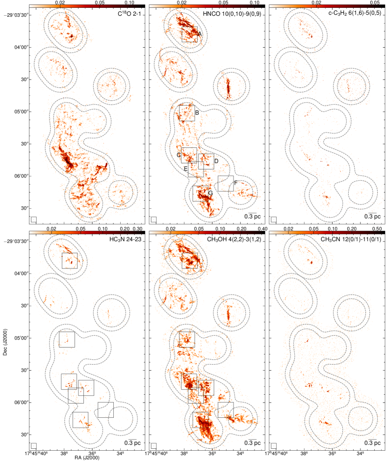
Figure 2: Continued.

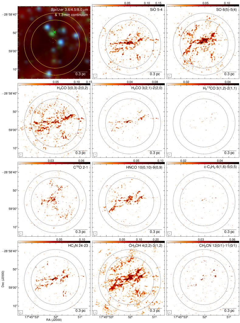
Figure 3: Molecular line emission in the 50 km s^-1 cloud. The layout of panels and symbols is the same as in Figure 2.

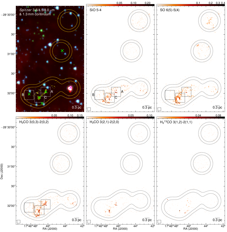
Figure 4: Molecular line emission in Sgr B1-off. The layout of panels and symbols is the same as in Figure 2.

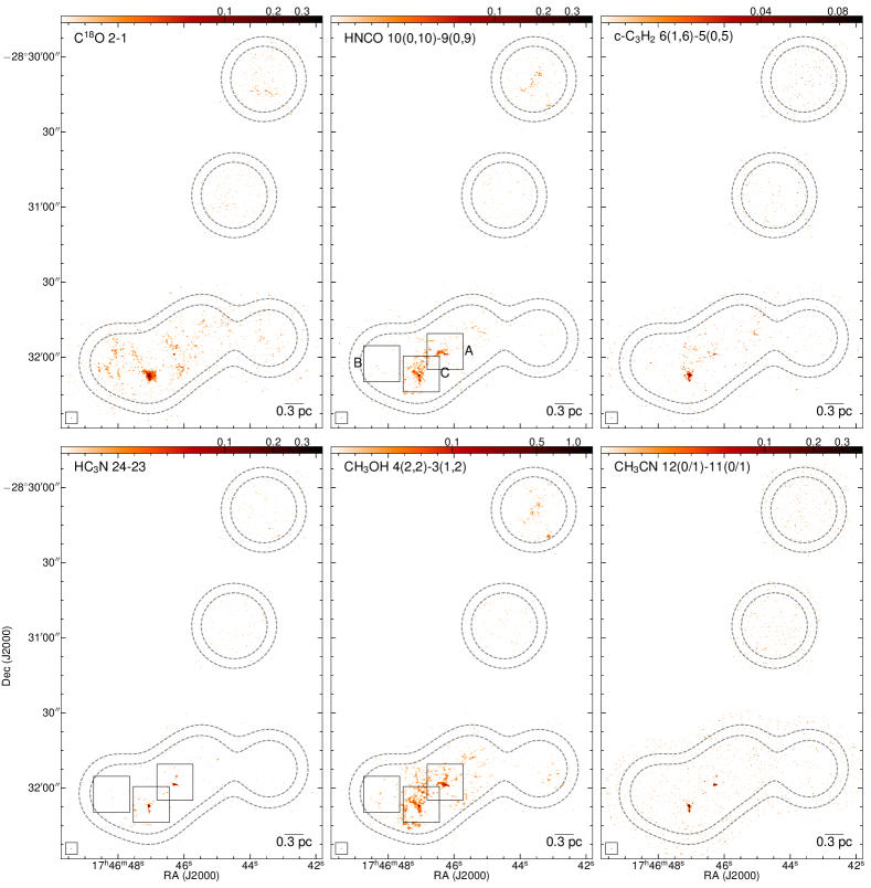
Figure 4: Continued.

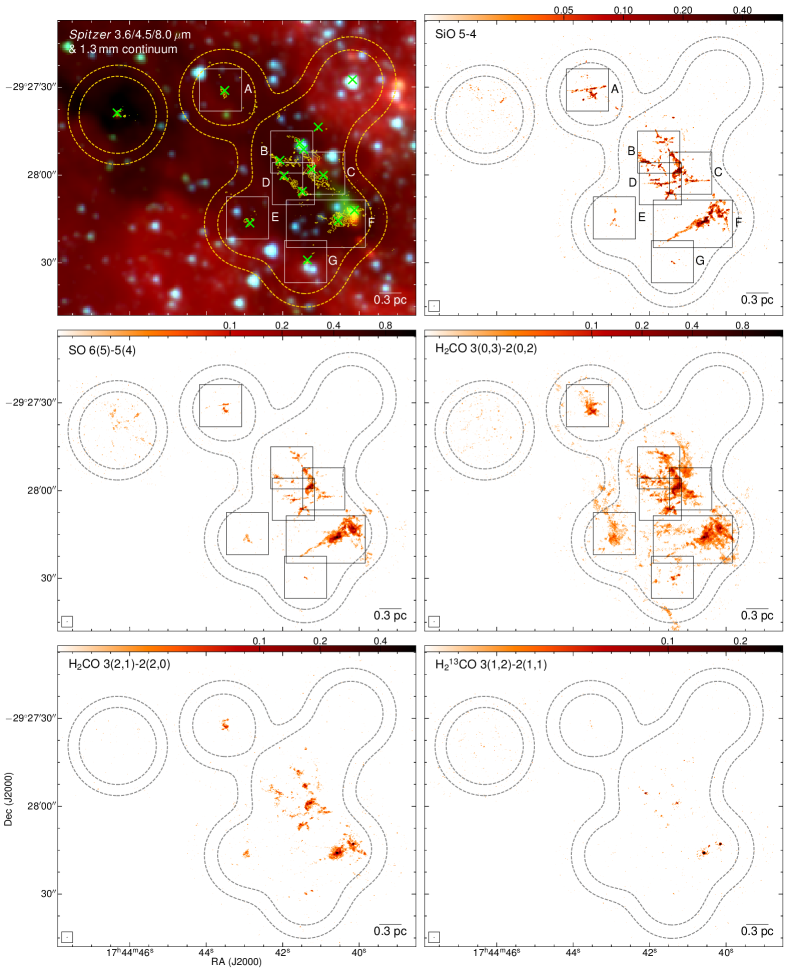
Figure 5: Molecular line emission in Sgr C. The layout of panels and symbols is the same as in Figure 2.

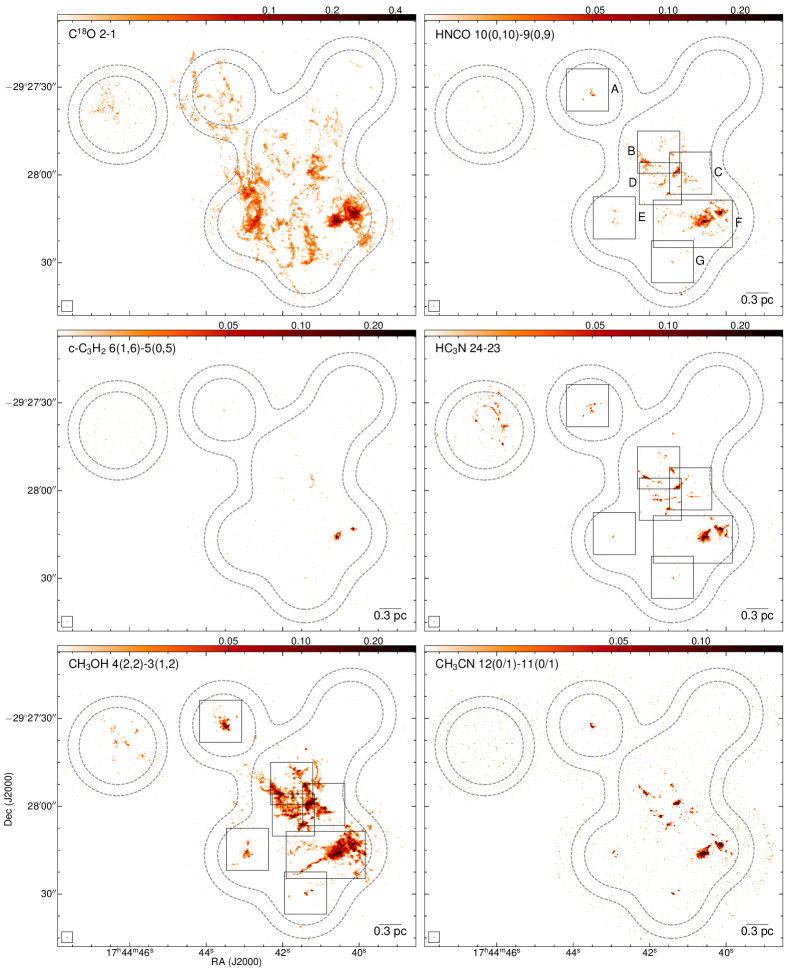
Figure 5: Continued.

3 RESULTS

3.1 Overview of the Line Emission

Typical spectra toward a chemically active core and a relatively quiescent region spatially offset from any cores but with line emission are shown in Figure 1. The former shows characteristic hot molecular core chemistry, while the latter represents regions that are likely influenced by pc scale shocks prevailing in the CMZ. Note that there exist even more chemically active cores (e.g., the two UC H ii regions in Sgr C), with many more spectral lines detected, mostly from complex organic molecules. Here, we focus on the spatially extended spectral line emission detected outside of the hot cores or UC H ii regions, and leave the discussion of the line-rich chemically active cores to a future paper.

We identified spatially extended line species, and plotted their integrated intensities in Figures 2–5. The line species include the CO isotopologue C¹⁸O, a group of potential shock tracers (SiO, SO, HNCO, CH₃OH), and several dense gas tracers that are sometimes found in outflows (H₂CO, H₂¹³CO, CH₃CN, c-C₃H₂, HC₃N). ¹³CO emission is more spatially extended than C¹⁸O and is not plotted. Three features are clearly seen: i) Linear structures spatially associated with dust emission are prominent, which may be outflow lobes (black boxes in the figures). ii) Multiple lines are tracing similar filamentary structures that are spatially offset from any dust emission, including some that are more typically confined to hot cores in environments outside of the CMZ (e.g., CH₃CN), whose nature is unclear. An example is marked by the blue arrow in Figure 2. iii) Point-like SiO emission with large linewidths ($>$20 km s^-1) is found toward two H₂O masers that have known AGB star counterparts (magenta crosses in Figures 2 & 4; see Lu et al. 2019a), with no associated dust emission within a radius of 0.1 pc, which is probably originated from the atmosphere of AGB stars (González Delgado et al., 2003). Here we focus on the first feature, potential outflows, while leaving the discussion of the other features to future papers.

The two CO isotopologue lines, ¹³CO and C¹⁸O, present strong absorption at velocities of $-$55, $-$30, and $-$5 km s^-1 against strong continuum emission (see the inset in Figure 1). These are consistent with the absorption features seen in other line observations toward the Galactic Center (e.g., Jones et al., 2012), and are attributed to foreground gas in spiral arms along the line of sight. In particular, the absorption at $-$55 km s^-1 is close to the cloud velocity of Sgr C, which complicates the interpretation of the two lines in Sgr C. Many of the lines, including H₂CO, CH₃OH, SiO, and the two CO isotopologues themselves, also present absorption features at a few km s^-1 blue-shifted with respect to the cloud velocity toward continuum emission peaks (e.g., the absorption at $\sim$12 km s^-1 in the inset of Figure 1). These features are likely owing to a combination of missing flux as a result of interferometer observations and self absorption when the lines become optically thick.

3.2 Identification of Outflows

Signatures of protostellar outflows have been detected toward Sgr B2(M) and (N), the two high-mass protoclusters in the Sgr B2 complex (Qin et al., 2008; Higuchi et al., 2015; Bonfand et al., 2017). Outside of Sgr B2, detecting protostellar outflows has been challenging in the CMZ, because of the lack of resolution to spatially resolve outflows and the prevalence of broad linewidth gas produced by phenomena other than outflows (Henshaw et al., 2019; Sormani et al., 2019). Previous Submillimeter Array (SMA) observations have detected widespread emission of potential shock tracers (e.g., SiO, SO, CH₃OH) at 0.2 pc scales in CMZ clouds (Kauffmann et al., 2013; Lu et al., 2017; Battersby et al., 2020). However, limited by the angular resolution and the imaging sensitivity, it was unclear whether the emission seen by the SMA is owing to protostellar outflows or pc-scale shocks prevailing in the CMZ. Only recently, ALMA observations with high resolution and high sensitivity start to detect outflows in the CMZ, e.g., in the G0.253$+$0.025 cloud (D. Walker et al. submitted, 2020).

Our high angular resolution ALMA observations resolved substructures of 2000 AU scale in the molecular line emission, enabling us to search for protostellar outflows. The integrated intensity maps in Figures 2–5 already reveal collimated emission spatially associated with cores, indicating the existence of outflows.

We then examined potential shock tracers detected by ALMA, including SiO, SO, H₂CO, HNCO, HC₃N, and CH₃OH. All these tracers have been previously found to be enhanced by at least one order of magnitude in shocked regions in protostellar outflows (e.g., Bachiller & Pérez Gutiérrez, 1997). We applied the following criteria to identify outflows:

i) We used the H₂O masers from Lu et al. (2019a) as a guidance to search for associated shock tracer emission. First, we made integrated intensity maps of SiO across the full velocity range, and searched for linear structures spatially associated with the masers. If linear emission is found, then, we made integrated intensity maps of blue and red shifted components based on the $V_{\text{lsr}}$ of the cloud (see Table 1), and checked whether the linear structures show symmetric blue and red shifted emission with respective to the masers. Finally, we determined the systematic velocity of each individual outflow driving source, by using dense gas tracers in the ALMA data toward the maser position (CH₃CN, HC₃N, CH₃OH, or C¹⁸O, in a decreasing order of preference; C¹⁸O was used only once, towards the 20 km s^-1 cloud-F #1), and remade integrated intensity maps of blue and red shifted components based on the individual $V_{\text{lsr}}$. If the shock tracer emission exhibits blue and red shifted components with respect to the systematic velocity at opposite positions to the maser position, it is considered as an outflow.

ii) In cases where H₂O masers are not present, we checked the emission of the six tracers around the 2000-AU scale cores from Paper I following the same procedures, to search for blue and/or red shifted line emission spatially offset from the cores. We require the blue and/or red shifted features to be seen in at least two shock tracers, including the canonical shock tracer SiO, plus any of the five supplemental tracers.

We identified 43 outflows, and marked regions where they are detected with boxes in Figures 2–5. The zoomed-in views are in Figures 6–22, in which we plot the red/blue shifted shock tracer emission with respect to the systematic velocity and highlight individual outflows with arrows. The position-velocity diagrams of the 43 outflows made from the SiO line are displayed in Figure 23. The numbers of outflows identified in the individual clouds are listed in Table 1.

In several cases, lobes from different outflows spatially overlap with each other (e.g., outflows #5–#9 in region C of the 20 km s^-1 cloud; see Figure 8), but we were able to separate them apart unambiguously based on velocities (see Figure 23). Most of the other outflows are easily distinguished spatially from nearby outflows and the diffuse emission. All these outflows are considered as ‘highly likely’. However, there exist cases where the outflows cannot be robustly separated from other outflows or the diffuse emission, either spatially or kinematically. One example is the two blue-shifted lobes in region B of the 20 km s^-1 cloud, where the lobes overlap in both projected locations and velocities (see Figures 7 & 23). Following the definitions in Li et al. (2020), we classified these ambiguous identifications as ‘candidates’. The classifications are noted with asterisks in Table 3, Figures 6–22, and Figure 23. Among the 43 outflows, 37 are highly likely, and 6 are candidates.

We stress that this visual identification is likely to be incomplete. Potential outflows could have been missed if they cannot be distinguished from the background emission or other outflows, or if their emission is too weak. The actual (in)completeness, however, is difficult to quantify, as the identification is based on visual inspection and is subjective in nature. Recent ALMA surveys toward infrared dark clouds in the Galactic disk using CO lines as the primary outflow tracer yield detection rates of 14%–22% (e.g., 62 out of 280 cores in Kong et al. 2019 and 41 out of 301 cores in Li et al. 2020 are identified with outflows). The detection rate using SiO as the primary tracer in this paper is 4–7% (Table 1), which is much lower. It is infeasible to directly compare, e.g., the outflow mass sensitivities of previous surveys and ours, considering that the observations use different lines as outflow tracers and assume different abundances. Assuming that the observations are sufficiently sensitive to detect all exiting outflows, the lower detection rate in our sample may suggest that we have missed a substantial number of outflows that are not traced by SiO, or may reflect the variation of outflow occurrence rates along the evolutionary stages.

Meanwhile, we also note that due to the complicated environment in the CMZ (e.g., the wide-spread shock tracer emission; Martín-Pintado et al., 1997) and possible contamination from the foreground, it is likely that false positive identifications exist in our sample if such large scale shock tracer emission accidentally lies upon cores. But such accidental spatial coincidence should be rare, as the velocities of the identified outflows and cores have a continuous overlap (Figure 23). Note that the cores associated with the outflows are all likely in the CMZ, given that the velocities of their line emission (e.g., C¹⁸O; see Figure 1 inset) are consistent with the overall velocity field in the CMZ (e.g., Henshaw et al., 2016), while spiral arm clouds along the line of sight are mostly seen as absorption in ¹³CO and C¹⁸O (Figure 1 inset), indicating that the overlapping spiral arm clouds consist of low-density gas and hence are unlikely to have dense cores.

SiO and SO seem to be the best outflow tracers among the six molecules. Their emission is usually well separated from the background, and is usually collimated as expected for outflows. CH₃OH, H₂CO, and HNCO often suffer from contamination from the background or foreground emission, and thus are not tracing the outflows as well as SiO and SO. HC₃N traces both cores and outflows. Its emission is weaker than the other molecules, therefore is not an optimized outflow tracer either. As pointed out by several previous studies, CH₃OH, H₂CO, HC₃N, and HNCO may be released into the gas phase by slow ($\lesssim$20 km s^-1) shocks that evaporate ice mantles of dust or be produced by gas phase reactions in post-shock regions, therefore probe the widespread low-velocity shocks in the CMZ (Lu et al., 2017; Tanaka et al., 2018; Taniguchi et al., 2018). SiO and SO, on the other hand, may be released from the dust by sputtering of the grain core, thus better probe fast ($\gtrsim$20 km s^-1) shocks induced by the outflows.

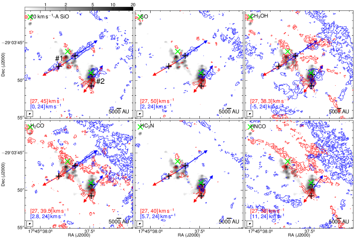
Figure 6: Outflows in region A in the 20 km s^-1 cloud. The gray scale image in all panels shows the ALMA 1.3 mm continuum emission, with the scale bar at the top in unit of mJy beam^-1 in a logarithmic scale. The green crosses mark positions of the H₂O masers in Lu et al. (2019a). In each panel, the blue and red contours illustrate the blue and red shifted line emission integrated within the specified velocity ranges, at levels of [3,6,12]$\sigma$, where $\sigma=\sqrt{N}\sigma_{c}v_{c}$, $N$ being the number of channel, $\sigma_{c}$ the rms of individual channels, and $v_{c}$ the channel width in km s^-1. When there are multiple outflows in the panel, the velocity ranges are chosen to highlight the bipolar morphologies of all the outflows, but for individual outflows, the blue and red shifted lobes may extend beyond these velocity ranges or be contaminated by diffuse gas, which can be better visualized in Figure 23. Identified outflows are highlighted by blue and red arrows, but note that some outflows are not seen in all the lines (in the case shown here, outflow #1 is not detected in HNCO). The thick black crosses mark the reference positions we choose to derive column densities of the molecules based on which we estimate molecular abundances.

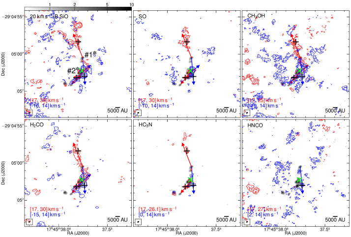
Figure 7: Outflows in region B in the 20 km s^-1 cloud.

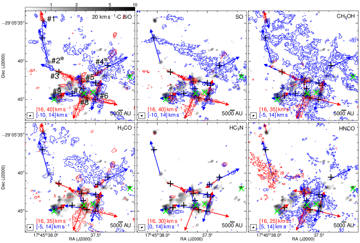
Figure 8: Outflows in region C in the 20 km s^-1 cloud.

Figure 9: Outflows in region D in the 20 km s^-1 cloud.

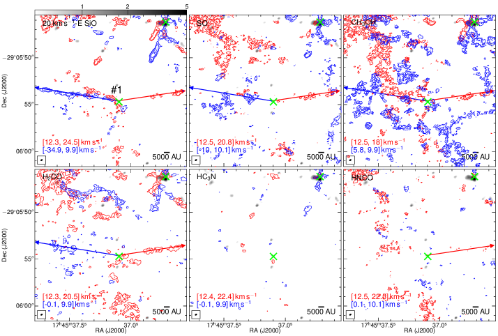
Figure 10: Outflows in region E in the 20 km s^-1 cloud.

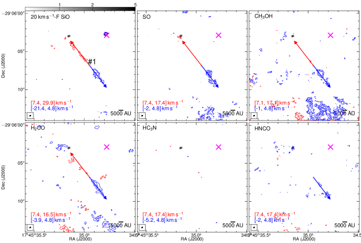
Figure 11: Outflows in region F in the 20 km s^-1 cloud.

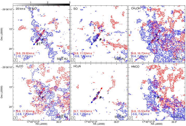
Figure 12: Outflows in region G in the 20 km s^-1 cloud.

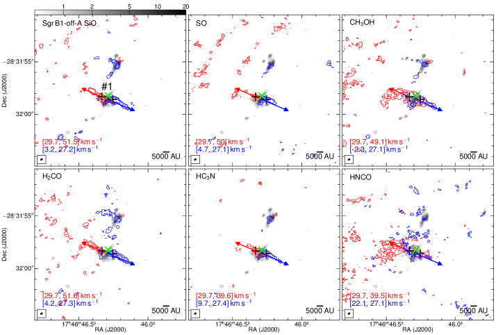
Figure 13: Outflows in region A in Sgr B1-off.

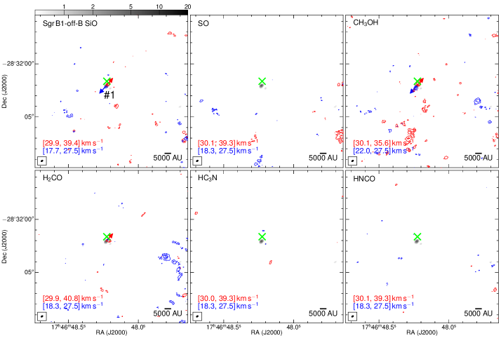
Figure 14: Outflows in region B in Sgr B1-off.

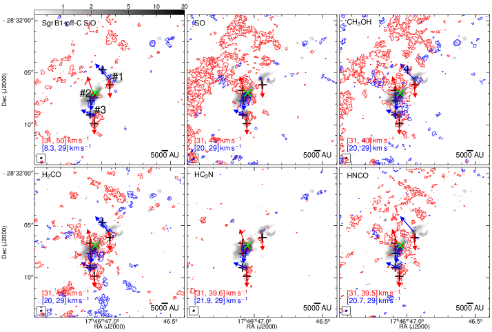
Figure 15: Outflows in region C in Sgr B1-off.

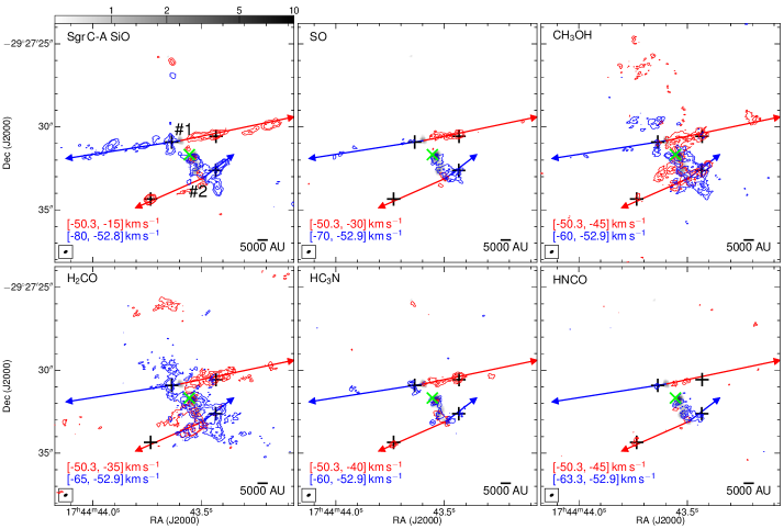
Figure 16: Outflows in region A in Sgr C.

Figure 17: Outflows in region B in Sgr C.

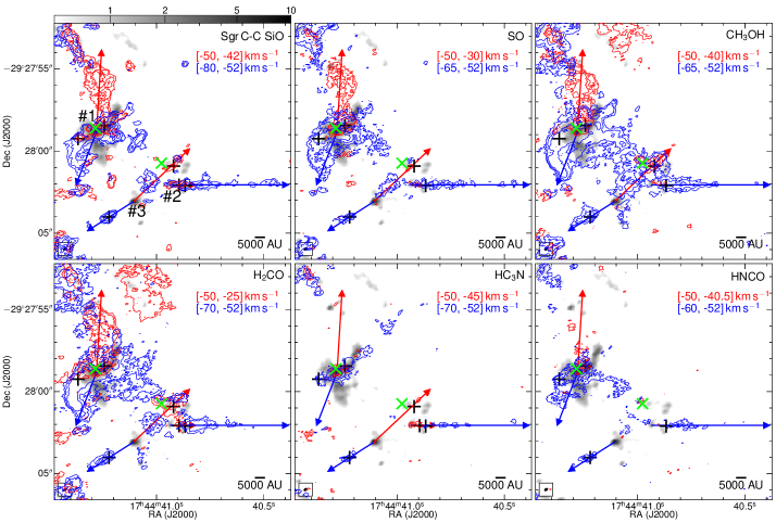
Figure 18: Outflows in region C in Sgr C.

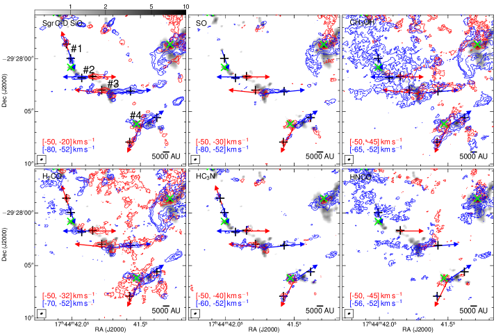
Figure 19: Outflows in region D in Sgr C.

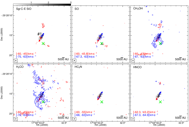
Figure 20: Outflows in region E in Sgr C.

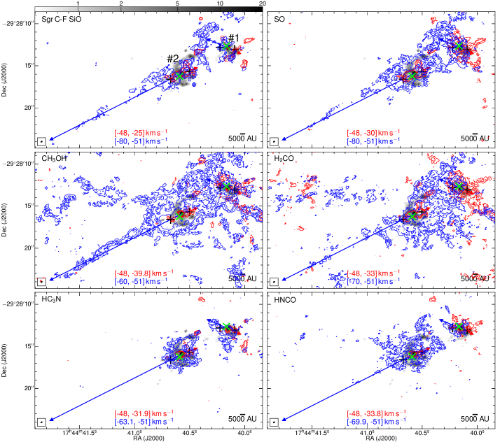
Figure 21: Outflows in region F in Sgr C.

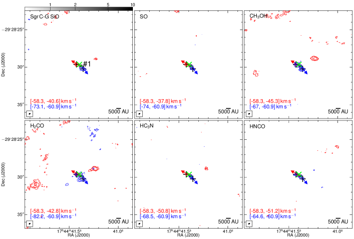
Figure 22: Outflows in region G in Sgr C.

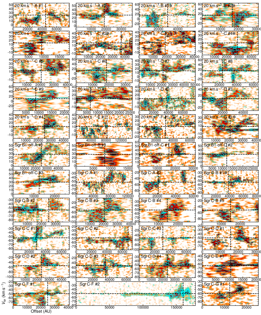
Figure 23: Position-velocity diagrams of the 43 outflows using the SiO line. The slices are taken along the arrows shown in Figures 6–22, from the blue-shifted to red-shifted side, averaged within a width of 5000 AU. The background image and the cyan contours show the SiO emission, with contour levels starting at 2$\sigma$ in step of 2$\sigma$ where $\sigma$$\approx$1 mJy beam^-1. The x axis is the spatial offset along the slices, and the y axis is $V_{\text{lsr}}$. The vertical and horizontal dashed lines mark the position and $V_{\text{lsr}}$ of the cores, respectively.

4 DISCUSSION

4.1 Estimate of Physical Properties of the Outflows

In this section, we calculate the column densities of the six molecules detected toward the identified outflows (Section 4.1.1), introduce the method to estimate the molecular abundances in the outflows (Section 4.1.2), and estimate the outflow masses, and where possible, the outflow energetics (Section 4.1.3). The uncertainties involved in the estimate of column densities, abundances, and masses are discussed in Section 4.1.4. We need an order-of-magnitude estimate on these parameters to discuss implications for astrochemistry and star formation in following sections, so the unavoidable significant uncertainties in these results (one to two orders of magnitude, as detailed in Section 4.1.4) are acceptable.

4.1.1 Column Densities of the Shock Tracers

We measure the molecular line integrated fluxes of the outflows in the primary beam corrected maps within a contour level of 3$\sigma$ for each line, and list the results in Table 3. The velocity range of the integration is chosen to start from one channel ($\sim$1.3 km s^-1) away from $V_{\text{lsr}}$ of the core to avoid diffuse emission around the system velocity, and end at the channel where the emission drops below 2$\sigma$. The separation of 1.3 km s^-1 should be able to role out most of the diffuse component as the FWHM linewidth at 0.1 pc scale in these clouds drops to this value and the linewidth at even smaller scales should be narrower (Kauffmann et al., 2017). The integrated fluxes should be lower limits given limited sensitivities and potential missed flux by the interferometer.

We then derive column densities with the measured fluxes, using the calcu toolkit (Li et al., 2020). Local thermodynamic equilibrium (LTE) conditions and optically thin line emission has been assumed. A constant excitation temperature of 70 K, which is the characteristic gas kinetic temperature in the CMZ (Ao et al., 2013; Ginsburg et al., 2016; Krieger et al., 2017), is assumed for all the lines. Note that the adopted temperature is different from that assumed for the dust in the cores in Paper I, 20 K. Observations show that the gas temperature at $\sim$0.1 pc scale in CMZ clouds is 70 K or even higher (Mills & Morris, 2013; Lu et al., 2017), while the dust temperature at this scale is largely unconstrained (see discussion in Paper I, ). Nevertheless, in Section 4.1.4 we find that the derived column densities are not sensitive to the choice of temperatures. Details of the column density calculation can be found in Appendix A.

We also select reference positions in the outflow lobes, and calculate the column densities. The reference positions must have detectable HC₃N emission, which we choose as the anchor molecule in the next section. The positions are adjusted to include emission of as many shock tracers as possible. A circle of 0$\farcs$3 across, comparable to the synthesized beam size, is used to define the area. The reference positions are marked by black crosses in Figures 6–22, and the derived column densities are listed in Table 3. The results are used to infer molecular abundances in the next section, and are further discussed in Section 4.2 in terms of astrochemical implications.

4.1.2 Molecular Abundances

In order to obtain the masses of the outflows, we must adopt an abundance for each shock tracer. However, the abundances of these molecules are known to be highly variable, especially toward the environment of our outflow sample with both strong shocks and complicated factors in the CMZ. One example is SiO, whose abundance has been found to vary by a factor of $>$$10^{5}$ across different regions (e.g., Martín-Pintado et al., 1997; Sanhueza et al., 2012; Csengeri et al., 2016; Li et al., 2019).

The dust emission is not always detected toward the outflows, so anchor molecules with relatively well-constrained abundances are often used to determine abundances of other molecules. One commonly used anchor molecule is CO and its isotopologues (e.g., Feng et al., 2016). By assuming a canonical ¹²CO abundance of 10^-4 with respect to H₂ (Blake et al., 1987), one might in principle use CO emission to derive the H₂ column density at a reference position in the outflow, and then determine the abundances of other molecules by dividing their column densities by the H₂ column density. However, in our data, the CO lines suffer from strong absorption and missing flux, and more importantly, morphologically they are not tracing the outflows seen in other molecules (Figures 2–5), probably because they are optically thick thus tracing the surface of the clouds instead of the outflows in the interior.

Therefore, we choose to anchor our estimate of molecular abundances on HC₃N, which is detected toward both cores and outflows and has shown a relatively stable abundance between the core/outflow environments in other observations (e.g., a factor of $\sim$30 enhancement from cores to outflow lobes around low-mass and high-mass protostars; Bachiller & Pérez Gutiérrez, 1997; Feng et al., 2016; Mendoza et al., 2018). The other molecules either show up only toward the outflows (e.g., SiO, SO) or suffer from contamination by pc-scale diffuse emission or strong absorption toward the cores (e.g., CH₃OH, H₂CO, and HNCO), and thus are not appropriate as the anchor tracer.

First, we compare the column densities of HC₃N and of H₂ toward the cores, and estimate abundances of HC₃N in the cores. The column densities of HC₃N is derived following the procedures in Section 4.1.1. The H₂ column densities are derived using the dust continuum from Paper I. Then we assume an enhancement of factor 30 (Bachiller & Pérez Gutiérrez, 1997; Feng et al., 2016), and obtain the abundances of HC₃N in the outflows. Finally we derive the H₂ column density in the outflows and use it to calibrate the abundances of the other shock tracers. The adopted molecular abundances with respect to molecular hydrogen are listed in Table 3, and the mean values of individual clouds are given in Table 1.

The estimated HC₃N abundances in the outflows are consistent in terms of the order of magnitude with previous result toward the 20 km s^-1 cloud using multiple HC₃N transitions ($10^{-9}$–$10^{-8}$ depending on the assumptions; Walmsley et al., 1986).

We note that the estimated abundances of the molecules span a large range. For example, the SiO abundance with respect to H₂ in our outflow sample ranges from 10^-10 to 10^-8, with a mean value of 2.05$\times$10^-9. This justifies our choice of estimating molecular abundances case by case, rather than assuming a constant abundance, for the latter case will bias the mass estimates significantly.

There are several cases where we cannot directly determine the abundance of a molecule in an outflow, and then we have to circumvent them by making reasonable assumptions: i) One lobe of an outflow has a well-defined reference position and the abundance can be determined from a scaling of the HC₃N emission, while the other lobe does not. In this case, we assume that the abundances of the blue/red-shifted lobes of the same outflow are identical and adopt the abundance of the other lobe. ii) An outflow has well-defined reference positions in multiple molecular line emission including HC₃N, but the core associated with it does not have detectable HC₃N emission, and therefore the abundance of HC₃N in the outflow cannot be determined. In this case, we adopt a mean HC₃N abundance of all the other outflows in the region, and then use it to determine abundances of other molecules in this outflow. iii) An outflow has well-defined reference positions in multiple molecular line emission, but not in HC₃N. We have to adopt mean molecular abundances of all the other outflows in the region for each of the detected molecules in the outflow. All these cases are explicitly noted in Table 3.

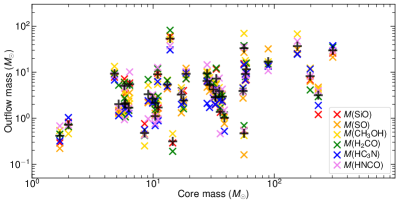
Figure 24: Outflow masses derived from different molecules, plotted against masses of the cores where the outflows originate. The outflow masses are the sum of those of the blue and red lobes, color-coded by molecular tracers based on which the masses are estimated. The systematic uncertainty of factor 70 in the outflow masses is not plotted here. The black crosses denote the mean outflow masses of the different molecules.

4.1.3 Masses and Energetics of the Outflows

After the molecular column densities and abundances are derived, the outflow masses are estimated by assuming uniform abundances within each outflow, using the calcu toolkit. The results are listed in Table 3, and plotted in Figure 24. For the same outflow lobe, multiple shock tracers could be detected, in which case we derive more than one outflow masses. All of these masses are deemed to be worth reporting, as the different molecules may trace different components of the same outflow with different chemical environments or excitation conditions. Nevertheless, the masses of the same outflow are consistent within an order of magnitude as demonstrated in Figure 24.

In a few cases where the outflow emission can be unambiguously separated from contaminations and the lobes are well collimated, we are able to measure the projected length and estimate a dynamical time-scale. Then the energetics of the outflows, e.g., the outflow rate and the outflow mechanical force, can be estimated following procedures in Li et al. (2020). One example of such well-defined outflows is the blue-shifted lobe of the Sgr C region F #2 outflow. With a projected angular scale of 20″ ($\sim$0.8 pc), and an outflow terminal velocity (the maximum velocity difference between the outflow and the core, as noted by the velocity range listed in Table 3) of 33.7 km s^-1, the dynamical time-scale is $3.2$$\times$$10^{4}$/$\cos$($\theta$) yr where $\theta$ is the inclination angle of the outflow lobe with respect to the plane of the sky. The outflow mass rate is then $\sim$$6$$\times$$10^{-4}$$\cos$($\theta$) $M_{\odot}$ yr^-1. If the inclination angle is not too large ($\theta$$<$80°), the outflow mass rate is $\gtrsim$$10^{-4}$ $M_{\odot}$ yr^-1, which is usually found toward outflows around high-mass young stellar objects (Maud et al., 2015). It is also possible to estimate the accretion rate, with the same assumptions in Li et al. (2020), e.g., a wind speed of 500 km s^-1 from the disk and a ratio between the accretion rate and the mass ejection rate of 3, which leads to a value of $2.5$$\times$$10^{-5}$$\cos$($\theta$) $M_{\odot}$ yr^-1. However, there are significant uncertainties in the outflow masses (see next section) and the true physical scale of the outflow lobes (contamination, potentially missed weak emission, inclination angle), on top of the unconstrained assumptions made in the calculation of the accretion rate (Li et al., 2020). We expect the uncertainty in the estimated outflow mass rate and accretion rate to be potentially three orders of magnitude or even greater, which is comparable to the dynamical range of our data (Figure 24). Therefore, we will not discuss these results further.

4.1.4 Uncertainties in the Estimated Parameters

There are several significant uncertainties in the estimate of column densities and outflow masses. First, we have assumed LTE conditions and a constant excitation temperature of 70 K when calculating the column densities. If we consider subthermal excitation, then the excitation temperature would be substantially lower than the kinetic temperature. If the temperature is varied between 20 and 100 K, a range that has been observed toward the CMZ (Ao et al., 2013; Ginsburg et al., 2016; Lu et al., 2017) and toward outflows in nearby clouds (Lefloch et al., 2012), then the resulting mass will vary by 60%, or 0.2 dex. Considering that the temperature could be even higher in post-shock regions ($\sim$10³ K; Tafalla et al., 2013), this uncertainty will only be larger. Second, we have assumed optically thin emission for all the molecular lines, while this may be invalid especially for CH₃OH and H₂CO, whose optical depths are higher than the other molecular lines as evidenced by the strong self absorption toward the cores. As shown in Figure 24, the masses of the same outflow estimated from different molecules are usually consistent within an order of magnitude. Therefore, the uncertainty in the outflow masses stemming from different optical depths of the molecular lines is estimated to be half of this range at most, or 0.5 dex. Third, as discussed in Section 2.2, the missing flux issue of the ALMA data may lead to an underestimate of 40% for the measured flux, or 0.15 dex. The three uncertainties above go into the calculation of column densities.

For outflow masses, the molecular abundances must be taken into account additionally. The abundances of these shock tracers hinge on that of HC₃N, which is again based on: i) the total molecular column densities in the cores that are derived from the dust continuum, with dependences on the assumed dust temperature, the dust opacity, and the gas-to-dust mass ratio (for detailed discussion, see Paper I, ), ii) the LTE condition assumed for the calculation of HC₃N column densities in the cores, which may not hold given the non-LTE excitation found in several CMZ clouds (Mills et al., 2018), and iii) the assumed enhancement of factor 30 of HC₃N from the core to the outflows. The estimated molecular abundances in the outflows usually span two orders of magnitude (Table 3). Therefore, we assign an uncertainty of one order of magnitude to the abundances, and note that the uncertainty is likely even greater.

Taken together, we estimate an uncertainty of 0.85 dex (a factor of 7) in the column densities, and an uncertainty of 1.85 dex (a factor of 70) in the outflow masses. These estimates are typical uncertainties for the individual outflows, though for particular outflows the uncertainties may be smaller or larger (e.g., for outflows where molecular abundances cannot be determined so mean abundances of the region are adopted, the uncertainties in the abundance and therefore the masses would be larger; for spatially compact outflows, the underestimate of the fluxes because of the missing flux issue would be less significant; for outflows with temperatures higher than 100 K, the uncertainties in the column densities and masses would be larger).

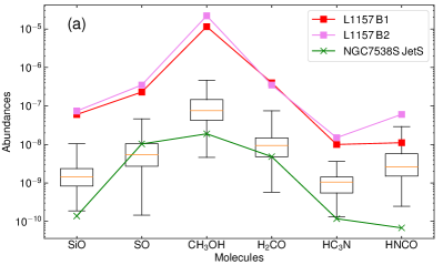
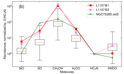
Figure 25: Absolute abundances of molecules with respect to H₂ in the outflows are plotted in (a), and those normalized with respect to the abundance of HC₃N are plotted in (b). Here we only consider the abundances with independent measurements but exclude those guessed from other outflows (i.e., entries with notes in the last column in Table 3). The boxes denote the first to third quartiles while the caps mark the full range of abundances in our outflow sample. The median of abundances of each molecule is marked by a horizontal orange line. The abundances of the low-mass outflow in L1157 and the high-mass outflow in NGC7538S are also plotted. The systematic uncertainties in the abundances are not plotted here.

4.2 Shock Chemistry in the Outflows

We compare the relative abundances of the six shock tracers and investigate the shock chemistry in the outflows. This is the first spatially resolved astrochemical study toward outflows in the CMZ, and one of the very few such studies even including works toward Galactic disk targets.

The abundances of the six shock tracers are presented in Figure 25. For each molecule, we plot the median of its abundances in all the outflows as a horizontal orange line.

To understand the relative abundances of the six molecules, we compare our result with similar studies toward nearby star forming clouds. However, we note that spatially resolved observations toward outflows that include all the six molecules, even for popular targets such as the Orion molecular cloud, are rare. For example, we are not able to find a paper that reports SiO, H₂CO, or HC₃N column densities or abundances in the explosive outflow around Orion KL, even though results of SO, CH₃OH, and HNCO are available (Feng et al., 2015). In the end, we are able to find only two representative outflows in nearby clouds: L1157, a well-studied, prototypical low-mass outflow around a low-mass protostar (e.g., Bachiller & Pérez Gutiérrez, 1997; Rodríguez-Fernández et al., 2010; Podio et al., 2017; Holdship et al., 2019), and NGC7538S, a prototypical massive outflow around a high-mass protostar (e.g., Naranjo-Romero et al., 2012; Feng et al., 2016).

We take the abundances of the six molecules toward L1157-B1 and B2 (two reference positions in the blue-shifted lobe) from Bachiller & Pérez Gutiérrez (1997) and Rodríguez-Fernández et al. (2010). For NGC7538S, we take the results from JetS, a reference position on the red-shifted side of the protostar, from Feng et al. (2016), except for SiO that is not observed by the authors. We instead obtain the SiO abundance at the reference position using data from Naranjo-Romero et al. (2012) (L. Zapata, private communications). The JetN position in Feng et al. (2016) does not show HC₃N emission, and therefore only an upper limit of its abundance can be detected, which prevents an appropriate comparison to our results as we use HC₃N to infer the abundances of the other molecules. All the results from the above publications have assumed LTE conditions and optically thin line emission. The abundances are plotted in Figure 25(a).

In addition, we note that the abundances toward L1157-B1/B2 are estimated based on CO lines, which may become optically thick and therefore result in overestimated abundances for other molecules (Bachiller & Pérez Gutiérrez, 1997). This may explain the systematically higher abundances for all the six molecules in L1157-B1/B2 than the other targets in Figure 25(a). To eliminate such biases, we normalize the abundances with respect to that of HC₃N in the outflows, and plot the relative abundances of the six molecules in Figure 25(b).

By comparing the two samples in Figure 25(b), the CMZ clouds vs. the two nearby clouds, we do not find clear evidence of difference between the relative abundances of the six shock tracers in the outflows. The relative abundances of the two nearby clouds usually fall within an order of magnitude apart from the medians of our CMZ outflow sample. However, given the significant uncertainty of the abundances and a limited sample from nearby clouds, it is premature to conclude any consistency between the two samples.

4.3 Implications for Star Formation and Chemistry

Protostellar outflows are ubiquitously detected in star forming regions, suggesting active gas accretion around protostars (e.g., Shang et al., 2007; Bally, 2016). Here we investigate star formation and chemistry in the four massive clouds in the CMZ based on our observations of the outflows.

The first implication, obviously, is that protostellar accretion disks ubiquituously exist in these clouds, as protostellar outflows are supposedly driven by disks (Shang et al., 2007). Direct observational evidence of protostellar accretion disks in the CMZ has been limited to the hot cores in the Sgr B2 cloud (e.g., Hollis et al., 2003; Higuchi et al., 2015), and even for these cases the evidence is ambiguous given the complicated kinematic environments in Sgr B2. More recently, D. Walker et al. (submitted, 2020) reported detection of protostellar outflows in G0.253$+$0.025 in the CMZ based on ALMA observations. Our finding of a large population of outflows (except in the 50 km s^-1 cloud, which is likely in a more evolved phase of star formation; Mills et al., 2011; Lu et al., 2019a), suggests that active accretion is ongoing around protostars in these CMZ clouds.

The second implication concerns the evolutionary phases of star formation in these clouds based on the statistics of the cores with or without star formation signatures. In Paper I, we identify 834 cores at 2000 AU scales in the three CMZ clouds. Among them, only 43 are found to be associated with outflows. The remaining 791 cores are not associated with other signatures of star formation (masers, H ii regions) either, and therefore are candidates of starless cores (gravitationally bound and prestellar, or simply unbound). However, as mentioned in Section 3.2, the outflow sample is very likely to be incomplete because of the subjectivity of the identification, thus potential outflows, even those with sufficiently strong emission, may have been missed. In addition, deeper observations may reveal more signatures of star formation such as weaker outflows or new masers. Therefore, the fraction of protostellar and starless cores is highly uncertain. For individual clouds, the fractions of cores associated with outflows range from 0.04 to 0.07 (Table 1), although this is unlikely to suggest any evolutionary trend among the three clouds given the small numbers of the outflow detections and the potential incompleteness of the outflow sample.

If we base our analysis on the current observations, i.e., 4–7% of the cores identified in Paper I are protostellar (Table 1), then we may put a constraint on the evolutionary phase of the clouds. The time scale needed to enter the protostellar phase is of the order 1–2 Myr for both low-mass and high-mass star forming cores (Enoch et al., 2008; Könyves et al., 2015; Battersby et al., 2017). This time scale is similar to the proposed lifetime of molecular clouds in the CMZ (Jeffreson et al., 2018; Barnes et al., 2020). Assuming that all the cores we detected will eventually evolve into the protostellar phase in a time scale of 1–2 Myr, the small fraction of the currently identified protostellar cores may suggest an age of star formation in these clouds as short as $\sim$0.05–0.1 Myr. In such case, star formation may have started only recently, if the clouds just condensed out of a more diffuse state, possibly driven by tidal compression during their arrival in the CMZ or on their orbit around the Galactic Center (Longmore et al., 2013b; Kruijssen et al., 2015, 2019), or by the impact of adjacent expanding H ii regions (Kendrew et al., 2013; Barnes et al., 2020). Again, we stress that this estimate depends on the (in)completeness of the outflow sample, and the age of star formation in these clouds is likely longer as the fraction of protostellar cores is potentially higher.

The third implication is related to the result presented in Figure 24, where we find outflows from both high-mass ($>$100 $M_{\odot}$) and low-mass ($<$5 $M_{\odot}$) cores. Here the core masses have a strong dependence on the unconstrained dust temperature and may be overestimated by a factor of 3, as demonstrated in Paper I. Several of the high-mass cores are known to be forming high-mass protostars, with UC H ii regions and class ii CH₃OH masers (Lu et al., 2019a, b). The low-mass cores, on the other hand, are only capable of forming low-mass stars with the current mass even assuming a high star formation efficiency of 50%. Meanwhile, the majority of the outflow masses lie in the range of 1–10 $M_{\odot}$, albeit with a large uncertainty of factor 70. This mass range is characteristically found around high-mass protostars (Zhang et al., 2005; Lu et al., 2018). Some of the outflows have lower masses of $<$1 $M_{\odot}$, which are typical for low-mass star forming regions (Arce et al., 2010). Therefore, considering the mass ranges of the cores and the outflows, the detected outflows likely trace a mix of high-mass and low-mass star formation. Simultaneous low-mass and high-mass star formation has been observed ubiquitously in massive clouds in the Galactic disk (e.g., Cyganowski et al., 2017; Pillai et al., 2019; Sanhueza et al., 2019), which we now confirm to take place in the CMZ as well.

The last implication, as discussed in Section 4.2, is about the shock chemistry in the outflows. Given the large uncertainties involved in the abundances (at least one order of magnitude), we are not able to conclude consistency between the shock chemistry in the CMZ clouds and in nearby analogs, but we do not find evidence of difference either. This is in contrast to the situation on the cloud scale of a few pc, where the chemistry in the CMZ is distinctly different from that in nearby clouds, e.g., an anomalous enhancement of complex organic molecules and shock tracers as compared to those in nearby clouds, suggesting the presence of wide-spread low-velocity shocks (Martín-Pintado et al., 1997; Requena-Torres et al., 2006; Menten et al., 2009). Several previous studies have pointed out that at the sub-0.1 pc scale, physical processes such as gas fragmentation and turbulent linewidths in the CMZ and in nearby regions may start to converge (e.g., Kauffmann et al. 2017; Lu et al. 2019a; Paper I; D. Walker et al. submitted, 2020) despite distinct properties on larger scales. Our results set the first step toward a similar comparison of the shock chemistry in protostellar outflows in the CMZ and in nearby clouds. Multi-transition spectral line observations toward the CMZ outflows that enable a more robust estimate of column densities and abundances, and a larger sample of resolved astrochemical studies toward outflows in nearby clouds, will help clarify whether the shock chemistry in the two environments are consistent or not.

5 CONCLUSIONS

As a follow-up of our Paper I, in which we used ALMA 1.3 mm continuum emission to study cores of 2000 AU scale in four massive clouds in the CMZ, we further use 1.3 mm molecular lines to identify protostellar outflows and investigate star formation activities associated with the cores. We choose six commonly used shock tracer molecules, including SiO, SO, CH₃OH, H₂CO, HC₃N, and HNCO. In three clouds (the 20 km s^-1 cloud, Sgr B1-off, and Sgr C), we identify 43 outflows traced by the six molecules, including 37 highly likely ones and 6 less likely ones that are considered as candidates. This is by far the largest sample of protostellar outflows identified in the CMZ. Then we estimate molecular abundances and masses of the outflows. Based on these findings and our previous studies (Lu et al. 2019a; Paper I), we conclude that:

• We find no evidence of differences between the physics (existence of accretion disks, Jeans fragmentation) and shock chemistry (relative abundances of the six shock tracer molecules in the outflows) in the sub-0.1 pc scale in the CMZ and in nearby clouds. Although on the cloud scale of a few pc, gas in the CMZ exhibits extraordinary physical and chemical properties as compared to gas in the Galactic disk or in nearby clouds, such as large turbulence linewidth, strong magnetic fields, and enhancements of particular molecules, in the smaller scale of $<$0.1 pc where gas starts to be self-gravitating, observed gas properties, and therefore physics and chemistry of the interstellar medium, may start to converge.

• Based on the identified star formation signatures associated with the cores, the fraction of protostellar cores in these clouds may be as low as $\sim$5%, which would indicate a short age of star formation of $\ll$1 Myr and a very early evolutionary phase for the three clouds, but this time scale is likely underestimated as our outflow sample is likely incomplete.

• Some of the identified outflows have small masses of $\lesssim$1 $M_{\odot}$ and are associated with low-mass cores of $\lesssim$5 $M_{\odot}$, and therefore likely trace low-mass star formation. Several high-mass outflows are associated with high-mass cores with known evidence of high-mass star formation. Therefore, low-mass and high-mass star formation are ongoing simultaneously in these clouds.

Appendix A Calculation of Molecular Column Densities

Assuming optically thin emission, negligible background, Rayleigh-Jeans approximation, and local thermodynamic equilibrium (LTE) conditions, the beam-averaged column density of a molecule can be derived following Mangum & Shirley (2015):

$$N_{\text{tot}}=\frac{8\pi k_{\text{B}}\nu^{2}}{hc^{3}A_{ul}}\frac{Q_{\text{rot}}}{g_{J}g_{K}g_{I}}\exp\left(\frac{E_{u}}{k_{\text{B}}T_{\text{ex}}}\right)\int T_{B}\text{d}v,$$ (A1)

where $k_{\text{B}}$ is the Boltzmann constant, $\nu$ is the rest frequency of the transition,$h$ is the Planck constant, $c$ is the speed of light, $A_{ul}$ is the spontaneous emission coefficient from the upper state $u$ to the lower state $l$, $Q_{\text{rot}}$ is the partition function of the molecule, $g_{i}$ ($i=J$, $K$, or $I$) are the degeneracies, $E_{u}$ is the energy of the upper state above the ground level, $T_{\text{ex}}$ is the excitation temperature, and $\int T_{B}\text{d}v$ is the integrated brightness temperature of the transition along the velocity axis. The spontaneous emission coefficient of the transition is

$$A_{ul}=\frac{64\pi^{4}\nu^{3}}{3hc^{3}}S\mu^{2},$$ (A2)

where $S$ is the line strength and $\mu$ is the permanent dipole moment of the molecule. Here we directly take the values of $A_{ul}$ from the LAMDA database (Schöier et al., 2005).

The partition functions $Q_{\text{rot}}$ are approximated using the equations in Mangum & Shirley (2015), as listed in Table 2. The rotation constants that are used in the calculation of $Q_{\text{rot}}$ are also listed in Table 2.

Then the column densities of the molecules are derived using Equation A1. The calculations are implemented in the calcu toolkit (Li et al., 2020).

Table 2: Transition spectral parameters of the outflow tracers.

Molecule	Transition	Frequency (GHz)	$E_{u}/k_{\text{B}}$ (K)	$A_{ul}$ (s-1)	$g_{J}$/$g_{K}$/$g_{I}$	$Q_{\text{rot}}$	Rotation Constants (MHz)
SiO	5–4	217.104919	31.3	5.197$\times$$10^{-4}$	11/1/1	$\frac{k_{\text{B}}T_{\text{ex}}}{hB_{0}}+\frac{1}{3}$	$B_{0}=21711.96$
HC3N	24–23	218.324723	131.0	0.826$\times$$10^{-3}$	49/1/1	"	$B_{0}=4549.059$
SO	6(5)–5(4)	219.949442	35.0	1.335$\times$$10^{-4}$	13/1/0.5	"	$B_{0}=21523.556$
H2CO	3(0,3)–2(0,2)	218.222192	21.0	2.818$\times$$10^{-4}$	7/1/0.25	$\frac{1}{2}\left(\frac{\pi k_{\text{B}}^{3}T_{\text{ex}}^{3}}{h^{3}A_{0}B_{0}C_{0}}\right)^{0.5}$	$A_{0}=281970.56$
							$B_{0}=38833.987$
							$C_{0}=34004.244$
CH3OH	4(2) –3(1)E1	218.440063	45.5	4.686$\times$$10^{-5}$	9/1/0.25	$\frac{1}{3}\left(\frac{\pi k_{\text{B}}^{3}T_{\text{ex}}^{3}}{h^{3}A_{0}B_{0}C_{0}}\right)^{0.5}$	$A_{0}=127523.4$
							$B_{0}=24690.2$
							$C_{0}=23759.7$
HNCO	10(0,10)–9(0,9)	219.798274	58.0	1.510$\times$$10^{-4}$	21/1/1	$\left(\frac{\pi k_{\text{B}}^{3}T_{\text{ex}}^{3}}{h^{3}A_{0}B_{0}C_{0}}\right)^{0.5}$	$A_{0}=912711.4$
							$B_{0}=11071.00$
							$C_{0}=10910.57$

Appendix B Observational and Physical Properties of the Outflows

The observational and physical properties of the identified outflows are listed in Table 3.

Table 3: Properties of the outflows.

ID	$V_{\text{lsr}}$	$M_{\text{core}}$	Lobes	$\Delta v$	$F_{\text{int}}$	$N_{\text{ref}}$	$X$	$M_{\text{out}}$	Notes
	(km s-1)	($M_{\odot}$)		(km s-1)	(Jy km s-1)	(cm-2)		($M_{\odot}$)
(1)	(2)	(3)	(4)	(5)	(6)	(7)	(8)	(9)	(10)
20 km s-1-A #1	24.7	13.1	SiO-blue	[1.5, 23.4]	2.83	1.12$\times$1014	1.29$\times$10-9	3.36
	[CH3CN]		SO-blue	[3.4, 23.5]	1.31	3.54$\times$1014	4.08$\times$10-9	3.46
			CH3OH-blue	[1.7, 23.4]	2.30	7.68$\times$1015	8.84$\times$10-8	4.73
			H2CO-blue	[2.8, 23.4]	1.89	6.32$\times$1014	7.27$\times$10-9	4.79
			HC3N-blue	[5.7, 23.4]	0.97	9.19$\times$1013	1.06$\times$10-9	3.96	$X$(HC3N) of #2
			HNCO-blue	$\cdots$	$\cdots$	$\cdots$	$\cdots$	$\cdots$
			SiO-red	[25.8, 42.1]	0.79	5.14$\times$1013	1.17$\times$10-9	1.03
			SO-red	[26.0, 31.5]	0.38	2.00$\times$1014	4.54$\times$10-9	0.90
			CH3OH-red	[26.0, 35.6]	0.73	2.92$\times$1015	6.64$\times$10-8	2.00
			H2CO-red	[25.9, 36.8]	0.61	2.76$\times$1014	6.28$\times$10-9	1.78
			HC3N-red	[26.0, 36.9]	0.22	4.65$\times$1013	1.06$\times$10-9	0.94	$X$(HC3N) of #2
			HNCO-red	$\cdots$	$\cdots$	$\cdots$	$\cdots$	$\cdots$
20 km s-1-A #2	27.1	197.6	SiO-blue	[$-$5.2, 25.9]	2.45	1.87$\times$1014	1.01$\times$10-9	3.72
	[CH3CN]		SO-blue	[2.0, 25.8]	2.03	1.20$\times$1015	6.54$\times$10-9	3.34
			CH3OH-blue	[$-$5.0, 25.8]	4.06	1.56$\times$1016	8.46$\times$10-8	8.71
			H2CO-blue	[4.2, 26.0]	0.36	7.23$\times$1014	3.92$\times$10-9	1.68
			HC3N-blue	[5.7, 26.1]	1.69	1.95$\times$1014	1.06$\times$10-9	6.79
			HNCO-blue	[20.7, 25.8]	0.28	2.04$\times$1014	1.11$\times$10-9	4.50
			SiO-red	[28.4, 74.5]	2.75	1.22$\times$1014	1.40$\times$10-9	3.01
			SO-red	[28.4, 51.5]	1.91	5.92$\times$1014	6.80$\times$10-9	3.01
			CH3OH-red	[28.4, 38.3]	1.19	5.30$\times$1015	6.09$\times$10-8	3.56
			H2CO-red	[28.4, 39.5]	1.13	7.49$\times$1014	8.60$\times$10-9	2.42
			HC3N-red	[28.4, 43.6]	1.21	9.21$\times$1013	1.06$\times$10-9	4.91
			HNCO-red	[28.4, 36.8]	0.33	1.46$\times$1014	1.68$\times$10-9	3.57
20 km s-1-B #1*	16.6	13.8	SiO-blue	[$-$36.3, 15.3]	4.61	3.11$\times$1014	3.08$\times$10-10	22.92
	[CH3OH]		SO-blue	[$-$11.3, 15.5]	1.34	3.58$\times$1014	3.54$\times$10-10	40.51
			CH3OH-blue	[$-$19.9, 15.3]	3.48	2.59$\times$1016	2.56$\times$10-8	24.69
			H2CO-blue	[$-$18.8, 15.3]	2.50	1.49$\times$1015	1.47$\times$10-9	31.29
			HC3N-blue	[$-$3.8, 15.3]	0.60	1.32$\times$1014	1.31$\times$10-10	19.85
			HNCO-blue	[2.0, 15.5]	0.55	5.30$\times$1014	5.24$\times$10-10	37.40
			SiO-red	[17.7, 39.4]	4.46	1.04$\times$1014	1.89$\times$10-10	36.19
			SO-red	[17.9, 28.8]	1.42	3.84$\times$1014	6.96$\times$10-10	21.84
			CH3OH-red	[17.9, 24.8]	0.68	2.55$\times$1015	4.62$\times$10-9	26.84
			H2CO-red	[17.7, 26.0]	1.58	3.18$\times$1014	5.77$\times$10-10	50.26
			HC3N-red	[17.8, 26.1]	0.33	7.20$\times$1013	1.31$\times$10-10	10.69
			HNCO-red	$\cdots$	$\cdots$	$\cdots$	$\cdots$	$\cdots$
20 km s-1-B #2*	15.1	27.9	SiO-blue	[$-$7.9, 13.8]	0.76	$\cdots$	5.81$\times$10-10	2.01	$X$(SiO) of the red lobe
	[CH3CN]		SO-blue	[8.7, 13.8]	0.04	$\cdots$	2.28$\times$10-9	0.18	$X$(SO) of the red lobe
			CH3OH-blue	[$-$7.7, 14.0]	0.93	$\cdots$	2.76$\times$10-8	6.09	$X$(CH3OH) of the red lobe
			H2CO-blue	[$-$10.7, 13.8]	0.89	$\cdots$	4.18$\times$10-9	3.92	$X$(H2CO) of the red lobe
			HC3N-blue	$\cdots$	$\cdots$	$\cdots$	$\cdots$	$\cdots$
			HNCO-blue	$\cdots$	$\cdots$	$\cdots$	$\cdots$	$\cdots$
			SiO-red	[16.4, 35.3]	1.73	1.39$\times$1014	5.81$\times$10-10	4.58
			SO-red	[16.4, 32.8]	0.96	5.46$\times$1014	2.28$\times$10-9	4.53
			CH3OH-red	[16.4, 27.5]	0.65	6.60$\times$1015	2.76$\times$10-8	4.24
			H2CO-red	[16.4, 31.4]	1.06	9.99$\times$1014	4.18$\times$10-9	4.64
			HC3N-red	[16.4, 26.1]	0.18	9.11$\times$1013	3.81$\times$10-10	2.10
			HNCO-red	$\cdots$	$\cdots$	$\cdots$	$\cdots$	$\cdots$
20 km s-1-C #1	13.9	35.8	SiO-blue	[$-$18.7, 12.6]	0.59	$\cdots$	1.44$\times$10-9	0.62	Mean $X$(SiO) of region C
	[CH3OH]		SO-blue	$\cdots$	$\cdots$	$\cdots$	$\cdots$	$\cdots$
			CH3OH-blue	[7.1, 12.6]	0.26	$\cdots$	8.41$\times$10-8	0.56	Mean $X$(CH3OH) of region C
			H2CO-blue	[1.5, 12.6]	0.26	$\cdots$	6.67$\times$10-9	0.71	Mean $X$(H2CO) of region C
			HC3N-blue	$\cdots$	$\cdots$	$\cdots$	$\cdots$	$\cdots$
			HNCO-blue	$\cdots$	$\cdots$	$\cdots$	$\cdots$	$\cdots$
			SiO-red	[15.0, 31.3]	0.67	$\cdots$	1.44$\times$10-9	0.72	Mean $X$(SiO) of region C
			SO-red	$\cdots$	$\cdots$	$\cdots$	$\cdots$	$\cdots$
			CH3OH-red	[15.2, 20.7]	0.67	$\cdots$	8.41$\times$10-8	1.44	Mean $X$(CH3OH) of region C
			H2CO-red	[15.0, 23.2]	0.35	$\cdots$	6.67$\times$10-9	0.97	Mean $X$(H2CO) of region C
			HC3N-red	$\cdots$	$\cdots$	$\cdots$	$\cdots$	$\cdots$
			HNCO-red	[15.2, 18.2]	0.03	$\cdots$	2.24$\times$10-9	0.46	Mean $X$(HNCO) of region C
20 km s-1-C #2*	16.6	17.1	SiO-blue	[$-$14.7, 15.3]	2.18	7.03$\times$1013	8.44$\times$10-10	3.96
	[CH3OH]		SO-blue	[6.0, 15.5]	0.29	2.00$\times$1014	2.40$\times$10-9	1.31
			CH3OH-blue	[$-$0.9, 15.3]	2.94	9.65$\times$1015	1.16$\times$10-7	4.59
			H2CO-blue	[0.1, 15.3]	1.03	4.02$\times$1014	4.83$\times$10-9	3.93
			HC3N-blue	[4.3, 15.3]	0.22	4.19$\times$1013	5.03$\times$10-10	1.99
			HNCO-blue	[$-$0.6, 15.5]	0.75	2.92$\times$1014	3.51$\times$10-9	3.79
			SiO-red	$\cdots$	$\cdots$	$\cdots$	$\cdots$	$\cdots$
			SO-red	$\cdots$	$\cdots$	$\cdots$	$\cdots$	$\cdots$
			CH3OH-red	$\cdots$	$\cdots$	$\cdots$	$\cdots$	$\cdots$
			H2CO-red	$\cdots$	$\cdots$	$\cdots$	$\cdots$	$\cdots$
			HC3N-red	$\cdots$	$\cdots$	$\cdots$	$\cdots$	$\cdots$
			HNCO-red	$\cdots$	$\cdots$	$\cdots$	$\cdots$	$\cdots$
20 km s-1-C #3	13.9	5.9	SiO-blue	[$-$13.3, 12.6]	1.09	$\cdots$	1.42$\times$10-9	1.18	$X$(SiO) of the red lobe
	[CH3OH]		SO-blue	$\cdots$	$\cdots$	$\cdots$	$\cdots$	$\cdots$
			CH3OH-blue	[8.5, 12.6]	0.02	$\cdots$	4.10$\times$10-8	0.10	$X$(CH3OH) of the red lobe
			H2CO-blue	$\cdots$	$\cdots$	$\cdots$	$\cdots$	$\cdots$
			HC3N-blue	$\cdots$	$\cdots$	$\cdots$	$\cdots$	$\cdots$
			HNCO-blue	$\cdots$	$\cdots$	$\cdots$	$\cdots$	$\cdots$
			SiO-red	[15.0, 74.5]	2.14	1.17$\times$1014	1.42$\times$10-9	2.31
			SO-red	[15.2, 30.2]	0.46	1.25$\times$1014	1.52$\times$10-9	3.26
			CH3OH-red	[15.2, 24.8]	0.25	3.38$\times$1015	4.10$\times$10-8	1.12
			H2CO-red	[15.0, 25.9]	0.30	4.20$\times$1014	5.10$\times$10-9	1.07
			HC3N-red	[15.1, 34.2]	0.18	4.15$\times$1013	5.04$\times$10-10	1.59	Mean $X$(HC3N) of region C
			HNCO-red	$\cdots$	$\cdots$	$\cdots$	$\cdots$	$\cdots$
20 km s-1-C #4*	11.2	4.8	SiO-blue	[$-$43.0, 9.9]	4.70	3.21$\times$1014	1.29$\times$10-9	5.58
	[CH3OH]		SO-blue	[$-$42.0, 10.1]	4.38	1.17$\times$1015	4.74$\times$10-9	9.92
			CH3OH-blue	[$-$9.1, 9.9]	2.10	7.08$\times$1015	2.85$\times$10-8	13.37
			H2CO-blue	[$-$9.3, 9.9]	1.75	1.07$\times$1015	4.31$\times$10-9	7.47
			HC3N-blue	[$-$6.5, 9.9]	0.75	1.25$\times$1014	5.04$\times$10-10	6.35	Mean $X$(HC3N) of region C
			HNCO-blue	[$-$6.0, 10.1]	0.76	3.92$\times$1014	1.58$\times$10-9	8.59
			SiO-red	[12.3, 61.0]	1.67	7.80$\times$1013	1.16$\times$10-9	2.20
			SO-red	$\cdots$	$\cdots$	$\cdots$	$\cdots$	$\cdots$
			CH3OH-red	$\cdots$	$\cdots$	$\cdots$	$\cdots$	$\cdots$
			H2CO-red	[12.3, 25.9]	0.36	2.46$\times$1014	3.66$\times$10-9	1.81
			HC3N-red	[12.4, 15.2]	0.02	3.39$\times$1013	5.04$\times$10-10	0.40	Mean $X$(HC3N) of region C
			HNCO-red	$\cdots$	$\cdots$	$\cdots$	$\cdots$	$\cdots$
20 km s-1-C #5	12.5	18.7	SiO-blue	[$-$39.0, 11.2]	1.03	9.12$\times$1013	4.37$\times$10-10	3.62
	[CH3CN]		SO-blue	[3.4, 11.5]	0.33	2.16$\times$1014	1.03$\times$10-9	3.42
			CH3OH-blue	[3.1, 11.3]	1.01	7.29$\times$1015	3.49$\times$10-8	5.24
			H2CO-blue	[1.5, 11.2]	0.13	2.91$\times$1014	1.39$\times$10-9	1.71
			HC3N-blue	[1.6, 11.2]	0.20	8.65$\times$1013	4.14$\times$10-10	1.93
			HNCO-blue	[6.0, 11.5]	0.43	3.40$\times$1014	1.63$\times$10-9	4.74
			SiO-red	[13.7, 42.1]	2.12	1.43$\times$1014	9.30$\times$10-10	3.49
			SO-red	[13.8, 24.8]	1.25	2.36$\times$1014	1.54$\times$10-9	8.75
			CH3OH-red	[13.8, 22.1]	1.07	8.52$\times$1015	5.54$\times$10-8	3.52
			H2CO-red	[13.7, 25.9]	1.55	7.95$\times$1014	5.17$\times$10-9	5.50
			HC3N-red	[13.8, 32.8]	0.73	6.37$\times$1013	4.14$\times$10-10	7.73
			HNCO-red	[13.8, 19.5]	0.68	3.37$\times$1014	2.19$\times$10-9	5.54
20 km s-1-C #6	12.5	89.0	SiO-blue	[$-$44.4, 11.2]	2.08	3.01$\times$1014	3.94$\times$10-10	8.12
	[CH3CN]		SO-blue	[$-$32.7, 11.5]	1.15	9.86$\times$1014	1.29$\times$10-9	9.54
			CH3OH-blue	[$-$13.2, 11.3]	1.26	1.49$\times$1016	1.95$\times$10-8	11.74
			H2CO-blue	[$-$26.9, 11.2]	0.86	1.49$\times$1015	1.95$\times$10-9	8.06
			HC3N-blue	[$-$13.3, 11.2]	0.62	2.07$\times$1014	2.71$\times$10-10	9.82
			HNCO-blue	[$-$2.0, 11.5]	0.25	5.11$\times$1014	6.69$\times$10-10	6.67
			SiO-red	[13.7, 34.0]	0.96	1.01$\times$1014	2.66$\times$10-10	5.53
			SO-red	[13.8, 24.8]	0.31	5.56$\times$1013	1.46$\times$10-10	22.54
			CH3OH-red	[13.8, 35.6]	0.71	9.70$\times$1015	2.55$\times$10-8	5.06
			H2CO-red	[13.7, 34.1]	1.09	1.10$\times$1015	2.89$\times$10-9	6.91
			HC3N-red	[13.8, 30.1]	0.24	1.03$\times$1014	2.71$\times$10-10	3.69
			HNCO-red	[13.8, 16.8]	0.06	9.40$\times$1013	2.47$\times$10-10	4.13
20 km s-1-C #7	15.1	29.2	SiO-blue	[$-$1.2, 13.8]	1.25	7.24$\times$1013	9.64$\times$10-10	1.98
	[CH3CN]		SO-blue	[0.7, 13.8]	0.94	4.48$\times$1014	5.96$\times$10-9	1.69
			CH3OH-blue	[4.4, 14.0]	2.05	1.23$\times$1016	1.64$\times$10-7	2.27
			H2CO-blue	[2.8, 13.8]	0.24	3.21$\times$1014	4.27$\times$10-9	1.01
			HC3N-blue	[5.7, 13.9]	0.32	8.40$\times$1013	1.12$\times$10-9	1.21
			HNCO-blue	[10.1, 13.8]	0.22	2.28$\times$1014	3.04$\times$10-9	1.31
			SiO-red	[16.4, 46.1]	3.52	9.16$\times$1013	1.45$\times$10-9	3.72
			SO-red	[16.4, 30.2]	2.21	6.94$\times$1014	1.10$\times$10-8	2.16
			CH3OH-red	[16.4, 27.5]	1.68	3.64$\times$1015	5.77$\times$10-8	5.29
			H2CO-red	[16.4, 30.0]	3.65	8.18$\times$1014	1.30$\times$10-8	5.17
			HC3N-red	[16.4, 22.0]	0.13	7.06$\times$1013	1.12$\times$10-9	0.50
			HNCO-red	[16.4, 23.5]	0.66	1.36$\times$1014	2.15$\times$10-9	5.48
20 km s-1-C #8	15.1	10.4	SiO-blue	[$-$10.6, 13.8]	1.36	8.97$\times$1013	4.12$\times$10-9	0.51
	[CH3CN]		SO-blue	[$-$10.0, 13.8]	1.31	4.74$\times$1014	2.18$\times$10-8	0.65
			CH3OH-blue	[$-$7.7, 14.0]	0.64	5.34$\times$1015	2.45$\times$10-7	0.48
			H2CO-blue	[$-$9.3, 13.8]	0.20	2.69$\times$1014	1.23$\times$10-8	0.30
			HC3N-blue	[9.7, 13.9]	0.07	7.45$\times$1012	3.42$\times$10-10	0.88
			HNCO-blue	$\cdots$	$\cdots$	$\cdots$	$\cdots$	$\cdots$
			SiO-red	[16.4, 47.5]	3.54	1.33$\times$1014	2.46$\times$10-9	2.20
			SO-red	[16.4, 38.2]	1.82	5.36$\times$1014	9.90$\times$10-9	1.97
			CH3OH-red	[16.4, 27.5]	0.50	3.22$\times$1015	5.95$\times$10-8	1.55
			H2CO-red	[16.4, 38.1]	1.41	7.75$\times$1014	1.43$\times$10-8	1.81
			HC3N-red	[16.4, 22.0]	0.12	1.85$\times$1013	3.42$\times$10-10	1.46
			HNCO-red	[16.4, 20.8]	0.18	1.61$\times$1014	2.98$\times$10-9	1.10
20 km s-1-C #9	11.1	10.4	SiO-blue	[$-$9.3, 9.8]	0.60	1.26$\times$1014	1.05$\times$10-9	0.89
	[HC3N]		SO-blue	[2.0, 10.1]	0.08	2.18$\times$1014	1.82$\times$10-9	0.48
			CH3OH-blue	[3.1, 9.9]	0.23	5.77$\times$1015	4.81$\times$10-8	0.87
			H2CO-blue	[1.5, 9.8]	0.30	5.64$\times$1014	4.70$\times$10-9	1.17
			HC3N-blue	[7.0, 9.8]	0.03	4.51$\times$1013	3.76$\times$10-10	0.32
			HNCO-blue	$\cdots$	$\cdots$	$\cdots$	$\cdots$	$\cdots$
			SiO-red	[12.3, 44.8]	0.75	1.45$\times$1014	2.92$\times$10-9	0.39
			SO-red	[12.4, 44.8]	0.99	8.00$\times$1014	1.61$\times$10-8	0.66
			CH3OH-red	[12.4, 20.7]	0.21	4.93$\times$1015	9.91$\times$10-8	0.38
			H2CO-red	[12.3, 27.3]	0.16	4.28$\times$1014	8.60$\times$10-9	0.35
			HC3N-red	[12.4, 16.6]	0.03	1.87$\times$1013	3.76$\times$10-10	0.37
			HNCO-red	[12.4, 16.8]	0.16	1.84$\times$1014	3.70$\times$10-9	0.76
20 km s-1-D #1	11.1	56.2	SiO-blue	$\cdots$	$\cdots$	$\cdots$	$\cdots$	$\cdots$
	[CH3CN]		SO-blue	$\cdots$	$\cdots$	$\cdots$	$\cdots$	$\cdots$
			CH3OH-blue	$\cdots$	$\cdots$	$\cdots$	$\cdots$	$\cdots$
			H2CO-blue	$\cdots$	$\cdots$	$\cdots$	$\cdots$	$\cdots$
			HC3N-blue	$\cdots$	$\cdots$	$\cdots$	$\cdots$	$\cdots$
			HNCO-blue	$\cdots$	$\cdots$	$\cdots$	$\cdots$	$\cdots$
			SiO-red	[12.3, 35.3]	1.35	$\cdots$	3.83$\times$10-9	0.54	Mean $X$(SiO) of region D
			SO-red	[12.4, 16.8]	0.25	$\cdots$	1.70$\times$10-8	0.16	Mean $X$(SO) of region D
			CH3OH-red	[12.4, 18.0]	0.40	$\cdots$	1.74$\times$10-7	0.42	Mean $X$(CH3OH) of region D
			H2CO-red	[12.3, 19.2]	0.63	$\cdots$	1.68$\times$10-8	0.69	Mean $X$(H2CO) of region D
			HC3N-red	$\cdots$	$\cdots$	$\cdots$	$\cdots$	$\cdots$
			HNCO-red	[12.4, 15.5]	0.17	$\cdots$	1.18$\times$10-8	0.53	Mean $X$(HNCO) of region D
20 km s-1-D #2	11.1	56.2	SiO-blue	[$-$21.4, 9.8]	8.95	2.03$\times$1014	1.01$\times$10-9	13.58
	[CH3CN]		SO-blue	[$-$20.7, 9.8]	8.28	6.64$\times$1014	3.30$\times$10-9	26.94
			CH3OH-blue	[$-$10.5, 9.9]	7.00	3.83$\times$1015	1.91$\times$10-8	66.50
			H2CO-blue	[$-$14.7, 9.8]	7.39	8.66$\times$1014	4.31$\times$10-9	31.52
			HC3N-blue	[$-$6.5, 9.8]	1.92	1.24$\times$1014	6.18$\times$10-10	13.33
			HNCO-blue	[$-$6.0, 9.8]	1.42	3.78$\times$1014	1.88$\times$10-9	26.99
			SiO-red	[12.3, 17.8]	0.47	5.56$\times$1013	3.97$\times$10-10	1.81
			SO-red	$\cdots$	$\cdots$	$\cdots$	$\cdots$	$\cdots$
			CH3OH-red	[12.4, 18.0]	1.28	9.72$\times$1015	6.93$\times$10-8	3.34
			H2CO-red	[12.3, 16.5]	0.99	4.10$\times$1014	2.92$\times$10-9	6.23
			HC3N-red	[12.4, 17.9]	0.16	8.66$\times$1013	6.18$\times$10-10	1.13
			HNCO-red	[12.4, 16.8]	0.39	2.43$\times$1014	1.73$\times$10-9	8.07
20 km s-1-D #3	9.9	35.1	SiO-blue	[$-$26.8, 8.6]	2.74	2.14$\times$1014	2.31$\times$10-9	1.82
	[CH3OH]		SO-blue	[$-$16.6, 8.8]	1.36	6.98$\times$1014	7.52$\times$10-9	1.95
			CH3OH-blue	[$-$1.0, 8.6]	1.10	4.58$\times$1015	4.94$\times$10-8	4.03
			H2CO-blue	[$-$2.6, 8.6]	0.59	3.39$\times$1014	3.65$\times$10-9	2.97
			HC3N-blue	[$-$1.1, 8.5]	0.46	8.20$\times$1013	8.84$\times$10-10	2.24	Mean $X$(HC3N) of region D
			HNCO-blue	[$-$0.6, 8.8]	0.62	2.77$\times$1014	2.99$\times$10-9	7.44
			SiO-red	[11.2, 38.0]	2.09	1.13$\times$1014	3.96$\times$10-9	0.81
			SO-red	[11.2, 23.5]	0.63	2.56$\times$1014	8.98$\times$10-9	0.75
			CH3OH-red	[11.2, 21.2]	0.14	1.24$\times$1015	4.35$\times$10-8	0.59
			H2CO-red	[11.0, 19.2]	0.11	2.10$\times$1014	7.37$\times$10-9	0.27
			HC3N-red	[11.1, 21.1]	0.05	2.52$\times$1013	8.84$\times$10-10	0.23	Mean $X$(HC3N) of region D
			HNCO-red	$\cdots$	$\cdots$	$\cdots$	$\cdots$	$\cdots$
20 km s-1-D #4	11.1	38.7	SiO-blue	[$-$7.9, 9.8]	2.03	9.71$\times$1013	3.53$\times$10-9	0.88
	[CH3CN]		SO-blue	[$-$3.3, 9.8]	0.68	3.84$\times$1014	1.40$\times$10-8	0.53
			CH3OH-blue	[$-$1.0, 9.9]	1.26	9.10$\times$1015	3.31$\times$10-7	0.69
			H2CO-blue	[$-$9.3, 9.8]	0.82	4.88$\times$1014	1.78$\times$10-8	0.84
			HC3N-blue	[3.0, 9.8]	0.08	3.17$\times$1013	1.15$\times$10-9	0.31
			HNCO-blue	[$-$0.6, 9.8]	0.25	3.90$\times$1014	1.42$\times$10-8	0.62
			SiO-red	[12.3, 38.0]	1.62	1.07$\times$1014	1.04$\times$10-8	0.24
			SO-red	[12.4, 22.2]	0.71	3.46$\times$1014	3.36$\times$10-8	0.23
			CH3OH-red	[12.4, 18.0]	0.52	2.86$\times$1015	2.77$\times$10-7	0.34
			H2CO-red	[12.3, 21.9]	0.77	4.33$\times$1014	4.20$\times$10-8	0.34
			HC3N-red	[12.4, 13.9]	0.05	1.19$\times$1013	1.15$\times$10-9	0.21
			HNCO-red	[12.4, 19.5]	0.72	3.01$\times$1014	2.92$\times$10-8	0.88
20 km s-1-E #1	11.2	5.8	SiO-blue	[$-$34.9, 9.9]	7.00	$\cdots$	1.69$\times$10-9	6.35	Mean $X$(SiO) of the cloud
	[CH3OH]		SO-blue	[$-$10.0, 10.1]	2.78	$\cdots$	7.10$\times$10-9	4.20	Mean $X$(SO) of the cloud
			CH3OH-blue	[5.8, 9.9]	0.24	$\cdots$	9.86$\times$10-8	0.45	Mean $X$(CH3OH) of the cloud
			H2CO-blue	[$-$0.1, 9.9]	1.49	$\cdots$	7.99$\times$10-9	3.42	Mean $X$(H2CO) of the cloud
			HC3N-blue	$\cdots$	$\cdots$	$\cdots$	$\cdots$	$\cdots$
			HNCO-blue	$\cdots$	$\cdots$	$\cdots$	$\cdots$	$\cdots$
			SiO-red	[12.3, 24.5]	0.88	$\cdots$	1.69$\times$10-9	0.79	Mean $X$(SiO) of the cloud
			SO-red	[12.5, 20.8]	1.27	$\cdots$	7.10$\times$10-9	1.92	Mean $X$(SO) of the cloud
			CH3OH-red	[12.5, 18.0]	0.55	$\cdots$	9.86$\times$10-8	1.02	Mean $X$(CH3OH) of the cloud
			H2CO-red	[12.3, 20.5]	1.11	$\cdots$	7.99$\times$10-9	2.57	Mean $X$(H2CO) of the cloud
			HC3N-red	$\cdots$	$\cdots$	$\cdots$	$\cdots$	$\cdots$
			HNCO-red	[12.5, 22.5]	0.56	$\cdots$	4.40$\times$10-9	4.54	Mean $X$(HNCO) of the cloud
20 km s-1-F #1	6.1	6.4	SiO-blue	[$-$21.4, 4.8]	3.39	$\cdots$	1.69$\times$10-9	3.08	Mean $X$(SiO) of the cloud
	[C18O]		SO-blue	[$-$2.0, 4.8]	1.54	$\cdots$	7.10$\times$10-9	2.34	Mean $X$(SO) of the cloud
			CH3OH-blue	[$-$1.0, 4.8]	1.26	$\cdots$	9.86$\times$10-8	2.32	Mean $X$(CH3OH) of the cloud
			H2CO-blue	[$-$3.9, 4.8]	1.51	$\cdots$	7.99$\times$10-9	3.48	Mean $X$(H2CO) of the cloud
			HC3N-blue	$\cdots$	$\cdots$	$\cdots$	$\cdots$	$\cdots$
			HNCO-blue	[$-$2.0, 4.8]	1.25	$\cdots$	4.40$\times$10-9	10.12	Mean $X$(HNCO) of the cloud
			SiO-red	[7.4, 29.9]	3.01	$\cdots$	1.69$\times$10-9	2.73	Mean $X$(SiO) of the cloud
			SO-red	[7.4, 17.4]	0.82	$\cdots$	7.10$\times$10-9	1.24	Mean $X$(SO) of the cloud
			CH3OH-red	[7.4, 17.4]	0.22	$\cdots$	9.86$\times$10-8	0.40	Mean $X$(CH3OH) of the cloud
			H2CO-red	[7.4, 16.5]	0.76	$\cdots$	7.99$\times$10-9	1.74	Mean $X$(H2CO) of the cloud
			HC3N-red	$\cdots$	$\cdots$	$\cdots$	$\cdots$	$\cdots$
			HNCO-red	$\cdots$	$\cdots$	$\cdots$	$\cdots$	$\cdots$
20 km s-1-G #1*	8.5	17.8	SiO-blue	[$-$12.0, 7.2]	1.28	6.93$\times$1013	1.28$\times$10-9	1.54
	[CH3CN]		SO-blue	[$-$0.6, 7.5]	1.03	3.40$\times$1014	6.28$\times$10-9	1.76
			CH3OH-blue	[0.4, 7.2]	1.12	1.00$\times$1016	1.85$\times$10-7	1.09
			H2CO-blue	$\cdots$	$\cdots$	$\cdots$	$\cdots$	$\cdots$
			HC3N-blue	[$-$4.3, 7.2]	0.29	7.72$\times$1013	1.43$\times$10-9	0.87
			HNCO-blue	$\cdots$	$\cdots$	$\cdots$	$\cdots$	$\cdots$
			SiO-red	[9.6, 29.9]	2.14	5.64$\times$1013	1.34$\times$10-9	2.44
			SO-red	[9.8, 11.5]	0.15	9.36$\times$1013	2.22$\times$10-9	0.75
			CH3OH-red	[9.8, 16.7]	0.60	6.68$\times$1015	1.59$\times$10-7	0.69
			H2CO-red	[9.6, 17.8]	0.74	3.58$\times$1014	8.52$\times$10-9	1.60
			HC3N-red	[9.7, 16.6]	0.46	6.00$\times$1013	1.43$\times$10-9	1.37
			HNCO-red	$\cdots$	$\cdots$	$\cdots$	$\cdots$	$\cdots$
Sgr B1-off-A #1	28.4	55.2	SiO-blue	[3.2, 27.2]	2.43	1.81$\times$1014	1.82$\times$10-9	2.06
	[CH3CN]		SO-blue	[4.7, 27.1]	1.24	7.34$\times$1014	7.40$\times$10-9	1.81
			CH3OH-blue	[$-$2.3, 27.1]	1.72	1.02$\times$1016	1.03$\times$10-7	3.05
			H2CO-blue	[4.2, 27.3]	1.56	1.11$\times$1015	1.12$\times$10-8	2.58
			HC3N-blue	[9.7, 27.4]	1.38	1.97$\times$1014	1.99$\times$10-9	2.98
			HNCO-blue	[22.1, 27.1]	0.18	1.64$\times$1014	1.65$\times$10-9	1.93
			SiO-red	[29.7, 51.5]	1.75	6.73$\times$1013	1.50$\times$10-9	1.79
			SO-red	[29.7, 50.2]	0.90	4.78$\times$1014	1.06$\times$10-8	0.92
			CH3OH-red	[29.7, 49.1]	1.31	6.57$\times$1015	1.46$\times$10-7	1.64
			H2CO-red	[29.7, 51.6]	1.02	6.77$\times$1014	1.51$\times$10-8	1.26
			HC3N-red	[29.7, 39.6]	0.72	8.93$\times$1013	1.99$\times$10-9	1.55
			HNCO-red	[29.7, 39.5]	0.64	2.91$\times$1014	6.47$\times$10-9	1.79
Sgr B1-off-B #1	28.8	14.5	SiO-blue	[17.7, 27.5]	0.15	$\cdots$	1.39$\times$10-9	0.16	Mean $X$(SiO) of the cloud
	[CH3OH]		SO-blue	$\cdots$	$\cdots$	$\cdots$	$\cdots$	$\cdots$
			CH3OH-blue	[22.0, 27.5]	0.09	$\cdots$	8.63$\times$10-8	0.20	Mean $X$(CH3OH) of the cloud
			H2CO-blue	$\cdots$	$\cdots$	$\cdots$	$\cdots$	$\cdots$
			HC3N-blue	$\cdots$	$\cdots$	$\cdots$	$\cdots$	$\cdots$
			HNCO-blue	$\cdots$	$\cdots$	$\cdots$	$\cdots$	$\cdots$
			SiO-red	[29.9, 39.4]	0.12	$\cdots$	1.39$\times$10-9	0.13	Mean $X$(SiO) of the cloud
			SO-red	$\cdots$	$\cdots$	$\cdots$	$\cdots$	$\cdots$
			CH3OH-red	[30.1, 35.6]	0.12	$\cdots$	8.63$\times$10-8	0.26	Mean $X$(CH3OH) of the cloud
			H2CO-red	[29.9, 40.8]	0.11	$\cdots$	1.09$\times$10-8	0.19	Mean $X$(H2CO) of the cloud
			HC3N-red	$\cdots$	$\cdots$	$\cdots$	$\cdots$	$\cdots$
			HNCO-red	$\cdots$	$\cdots$	$\cdots$	$\cdots$	$\cdots$
Sgr B1-off-C #1	30.0	30.6	SiO-blue	[8.3, 28.7]	0.46	$\cdots$	1.66$\times$10-9	0.42	$X$(SiO) of the red lobe
	[HC3N]		SO-blue	$\cdots$	$\cdots$	$\cdots$	$\cdots$	$\cdots$
			CH3OH-blue	[22.0, 28.9]	0.15	$\cdots$	5.39$\times$10-8	0.50	$X$(CH3OH) of the red lobe
			H2CO-blue	[11.0, 28.7]	0.52	$\cdots$	1.11$\times$10-8	0.87	$X$(H2CO) of the red lobe
			HC3N-blue	$\cdots$	$\cdots$	$\cdots$	$\cdots$	$\cdots$
			HNCO-blue	[24.7, 28.8]	0.09	$\cdots$	5.41$\times$10-9	0.29	$X$(HNCO) of the red lobe
			SiO-red	[31.2, 51.5]	0.55	8.64$\times$1013	1.66$\times$10-9	0.51
			SO-red	[31.3, 47.5]	0.19	2.84$\times$1014	5.44$\times$10-9	0.38
			CH3OH-red	[31.3, 39.7]	0.24	2.81$\times$1015	5.39$\times$10-8	0.81
			H2CO-red	[31.3, 47.5]	0.63	5.78$\times$1014	1.11$\times$10-8	1.05
			HC3N-red	[31.3, 38.2]	0.17	3.40$\times$1013	6.52$\times$10-10	1.10
			HNCO-red	[31.3, 39.5]	0.16	2.82$\times$1014	5.41$\times$10-9	0.53
Sgr B1-off-C #2	29.7	230.4	SiO-blue	[20.5, 28.6]	0.51	5.13$\times$1013	1.01$\times$10-9	0.78
	[CH3CN]		SO-blue	[20.7, 28.4]	0.77	4.52$\times$1014	8.86$\times$10-9	0.94
			CH3OH-blue	[19.3, 28.4]	0.27	4.90$\times$1015	9.61$\times$10-8	0.51
			H2CO-blue	[11.0, 28.7]	0.44	4.61$\times$1014	9.04$\times$10-9	0.90
			HC3N-blue	[24.6, 28.4]	0.20	5.34$\times$1013	1.05$\times$10-9	0.80
			HNCO-blue	[24.7, 28.4]	0.17	1.52$\times$1014	2.98$\times$10-9	1.02
			SiO-red	[31.0, 35.3]	0.27	$\cdots$	1.01$\times$10-9	0.42	$X$(SiO) of the blue lobe
			SO-red	[31.0, 36.8]	0.95	2.20$\times$1014	2.72$\times$10-9	3.78
			CH3OH-red	[31.0, 35.6]	0.98	3.80$\times$1015	4.70$\times$10-8	3.79
			H2CO-red	[31.0, 40.8]	0.64	4.69$\times$1014	5.80$\times$10-9	2.04
			HC3N-red	[31.0, 38.2]	0.27	8.47$\times$1013	1.05$\times$10-9	1.09
			HNCO-red	[31.0, 36.8]	0.66	3.29$\times$1014	4.07$\times$10-9	2.91
Sgr B1-off-C #3	30.0	32.6	SiO-blue	[17.7, 28.7]	0.28	5.22$\times$1013	9.50$\times$10-10	0.46
	[HC3N]		SO-blue	[19.4, 28.8]	0.16	2.32$\times$1014	4.22$\times$10-9	0.42
			CH3OH-blue	[17.9, 28.9]	0.32	4.16$\times$1015	7.57$\times$10-8	0.78
			H2CO-blue	[17.7, 28.7]	0.36	6.18$\times$1014	1.12$\times$10-8	0.60
			HC3N-blue	[21.9, 28.8]	0.12	7.08$\times$1013	1.29$\times$10-9	0.38
			HNCO-blue	[20.7, 28.8]	0.27	3.08$\times$1014	5.61$\times$10-9	0.86
			SiO-red	[31.2, 46.0]	1.38	9.48$\times$1013	1.42$\times$10-9	1.50
			SO-red	[31.3, 44.9]	1.01	2.72$\times$1014	4.06$\times$10-9	2.69
			CH3OH-red	[31.3, 42.4]	0.92	5.52$\times$1015	8.25$\times$10-8	2.04
			H2CO-red	[31.3, 42.2]	1.81	8.52$\times$1014	1.27$\times$10-8	2.64
			HC3N-red	[31.3, 39.6]	0.49	8.62$\times$1013	1.29$\times$10-9	1.62
			HNCO-red	[31.3, 38.2]	0.73	2.72$\times$1014	4.07$\times$10-9	3.20
Sgr C-A #1	$-$51.6	10.9	SiO-blue	[$-$74.4, $-$52.8]	4.94	5.40$\times$1013	1.60$\times$10-9	4.71
	[CH3CN]		SO-blue	[$-$64.6, $-$52.9]	1.48	2.12$\times$1014	6.28$\times$10-9	2.53
			CH3OH-blue	[$-$58.9, $-$52.9]	0.57	2.04$\times$1015	6.05$\times$10-8	1.69
			H2CO-blue	[$-$64.6, $-$52.9]	0.62	6.26$\times$1014	1.86$\times$10-8	0.61
			HC3N-blue	[$-$57.7, $-$52.9]	0.59	3.73$\times$1013	1.11$\times$10-9	2.27
			HNCO-blue	[$-$63.3, $-$52.9]	0.33	4.42$\times$1014	1.31$\times$10-8	0.45
			SiO-red	[$-$50.3, $-$17.7]	4.86	1.92$\times$1014	1.55$\times$10-9	4.79
			SO-red	[$-$50.3, $-$28.5]	2.25	5.36$\times$1014	4.32$\times$10-9	5.58
			CH3OH-red	[$-$50.3, $-$41.2]	0.84	5.04$\times$1015	4.07$\times$10-8	3.75
			H2CO-red	[$-$50.3, $-$38.8]	2.96	5.95$\times$1014	4.81$\times$10-9	11.26
			HC3N-red	[$-$50.3, $-$40.0]	1.04	1.37$\times$1014	1.11$\times$10-9	3.99
			HNCO-red	[$-$50.3, $-$44.5]	0.28	4.93$\times$1013	3.98$\times$10-10	12.26
Sgr C-A #2	$-$51.6	5.2	SiO-blue	[$-$81.2, $-$52.8]	2.06	1.28$\times$1014	6.65$\times$10-9	0.47
	[CH3CN]		SO-blue	[$-$72.6, $-$52.9]	1.02	3.92$\times$1014	2.04$\times$10-8	0.53
			CH3OH-blue	[$-$61.6, $-$52.9]	1.46	8.41$\times$1015	4.37$\times$10-7	0.60
			H2CO-blue	[$-$68.6, $-$52.9]	1.93	1.09$\times$1015	5.67$\times$10-8	0.62
			HC3N-blue	[$-$60.4, $-$52.9]	0.34	4.91$\times$1013	2.55$\times$10-9	0.57
			HNCO-blue	[$-$63.3, $-$52.9]	0.25	3.37$\times$1014	1.75$\times$10-8	0.25
			SiO-red	[$-$50.3, 9.3]	4.40	2.48$\times$1014	7.59$\times$10-9	0.89
			SO-red	[$-$50.3, $-$37.8]	0.49	1.81$\times$1014	5.54$\times$10-9	0.95
			CH3OH-red	[$-$50.3, $-$45.3]	0.28	2.59$\times$1015	7.93$\times$10-8	0.65
			H2CO-red	[$-$50.3, $-$33.3]	1.64	2.15$\times$1014	6.58$\times$10-9	4.58
			HC3N-red	[$-$50.3, $-$42.7]	0.33	8.34$\times$1013	2.55$\times$10-9	0.56
			HNCO-red	[$-$50.3, $-$45.8]	0.34	1.39$\times$1014	4.25$\times$10-9	1.43
Sgr C-B #1*	$-$53.4	11.0	SiO-blue	[$-$59.6, $-$54.7]	0.12	$\cdots$	1.68$\times$10-9	0.11	$X$(SiO) of the red lobe
	[CH3OH]		SO-blue	[$-$64.6, $-$54.7]	0.14	$\cdots$	5.44$\times$10-9	0.28	$X$(SO) of the red lobe
			CH3OH-blue	[$-$60.2, $-$54.7]	0.31	$\cdots$	8.17$\times$10-8	0.69	$X$(CH3OH) of the red lobe
			H2CO-blue	[$-$68.6, $-$54.7]	0.31	$\cdots$	8.78$\times$10-9	0.64	$X$(H2CO) of the red lobe
			HC3N-blue	$\cdots$	$\cdots$	$\cdots$	$\cdots$	$\cdots$
			HNCO-blue	[$-$56.6, $-$54.7]	0.02	$\cdots$	2.15$\times$10-9	0.21	$X$(HNCO) of the red lobe
			SiO-red	[$-$52.1, $-$39.3]	1.70	7.96$\times$1013	1.68$\times$10-9	1.55
			SO-red	[$-$52.1, $-$45.8]	0.50	2.58$\times$1014	5.44$\times$10-9	0.98
			CH3OH-red	[$-$52.1, $-$46.6]	0.80	3.87$\times$1015	8.17$\times$10-8	1.77
			H2CO-red	[$-$52.4, $-$40.1]	1.13	4.16$\times$1014	8.78$\times$10-9	2.36
			HC3N-red	[$-$52.3, $-$45.4]	0.18	4.07$\times$1013	8.59$\times$10-10	0.88
			HNCO-red	[$-$52.1, $-$48.5]	0.09	1.02$\times$1014	2.15$\times$10-9	0.75
Sgr C-B #2	$-$54.9	2.0	SiO-blue	[$-$66.3, $-$56.2]	1.17	4.64$\times$1013	3.37$\times$10-9	0.53
	[HC3N]		SO-blue	[$-$63.3, $-$56.2]	0.68	2.40$\times$1014	1.74$\times$10-8	0.42
			CH3OH-blue	[$-$64.3, $-$56.1]	1.18	6.38$\times$1015	4.63$\times$10-7	0.46
			H2CO-blue	[$-$75.4, $-$56.2]	2.05	7.78$\times$1014	5.65$\times$10-8	0.66
			HC3N-blue	[$-$63.1, $-$56.2]	0.44	3.41$\times$1013	2.47$\times$10-9	0.77
			HNCO-blue	[$-$60.6, $-$56.2]	0.24	8.27$\times$1013	6.00$\times$10-9	0.71
			SiO-red	[$-$53.6, $-$31.2]	0.72	8.91$\times$1013	3.84$\times$10-9	0.29
			SO-red	[$-$53.9, $-$37.8]	0.40	4.44$\times$1014	1.91$\times$10-8	0.22
			CH3OH-red	$\cdots$	$\cdots$	$\cdots$	$\cdots$	$\cdots$
			H2CO-red	$\cdots$	$\cdots$	$\cdots$	$\cdots$	$\cdots$
			HC3N-red	[$-$53.6, $-$44.0]	0.15	5.74$\times$1013	2.47$\times$10-9	0.26
			HNCO-red	$\cdots$	$\cdots$	$\cdots$	$\cdots$	$\cdots$
Sgr C-B #3	$-$50.2	27.9	SiO-blue	[$-$140.6, $-$51.4]	4.16	4.17$\times$1014	1.62$\times$10-9	3.92
	[CH3CN]		SO-blue	[$-$126.0, $-$51.2]	2.88	2.34$\times$1015	9.12$\times$10-9	3.38
			CH3OH-blue	[$-$64.3, $-$51.5]	1.24	8.23$\times$1015	3.21$\times$10-8	7.00
			H2CO-blue	[$-$114.6, $-$51.5]	2.88	3.66$\times$1015	1.43$\times$10-8	3.69
			HC3N-blue	[$-$75.3, $-$51.5]	0.56	2.22$\times$1014	8.65$\times$10-10	2.78
			HNCO-blue	[$-$68.6, $-$51.2]	0.93	3.99$\times$1014	1.55$\times$10-9	10.63
			SiO-red	[$-$48.9, 45.8]	3.53	3.27$\times$1014	1.12$\times$10-9	4.82
			SO-red	[$-$48.9, 15.6]	1.88	1.12$\times$1015	3.86$\times$10-9	5.22
			CH3OH-red	[$-$48.9, $-$23.6]	0.84	1.51$\times$1016	5.18$\times$10-8	2.93
			H2CO-red	[$-$48.9, 4.5]	3.02	3.51$\times$1015	1.20$\times$10-8	4.61
			HC3N-red	[$-$48.9, $-$14.3]	0.72	2.52$\times$1014	8.65$\times$10-10	3.57
			HNCO-red	[$-$48.9, $-$45.8]	0.10	1.32$\times$1014	4.53$\times$10-10	3.86
Sgr C-B #4	$-$50.8	5.8	SiO-blue	[$-$75.8, $-$52.1]	0.58	1.47$\times$1014	2.30$\times$10-9	0.39
	[HC3N]		SO-blue	[$-$67.3, $-$52.1]	0.18	2.90$\times$1014	4.54$\times$10-9	0.43
			CH3OH-blue	[$-$60.2, $-$52.0]	0.41	3.82$\times$1015	5.98$\times$10-8	1.23
			H2CO-blue	[$-$68.6, $-$52.1]	0.31	7.24$\times$1014	1.13$\times$10-8	0.50
			HC3N-blue	[$-$59.0, $-$52.1]	0.04	4.17$\times$1013	6.52$\times$10-10	0.27
			HNCO-blue	$\cdots$	$\cdots$	$\cdots$	$\cdots$	$\cdots$
			SiO-red	[$-$49.5, $-$32.5]	0.64	7.55$\times$1013	7.27$\times$10-10	1.35
			SO-red	[$-$49.5, $-$37.8]	0.20	2.50$\times$1014	2.40$\times$10-9	0.91
			CH3OH-red	[$-$49.5, $-$41.2]	0.52	3.85$\times$1015	3.71$\times$10-8	2.53
			H2CO-red	[$-$49.7, $-$38.8]	0.80	6.85$\times$1014	6.60$\times$10-9	2.22
			HC3N-red	[$-$49.5, $-$41.3]	0.22	6.77$\times$1013	6.52$\times$10-10	1.46
			HNCO-red	[$-$49.5, $-$47.2]	0.06	1.15$\times$1014	1.11$\times$10-9	0.93
Sgr C-B #5	$-$50.7	1.7	SiO-blue	[$-$97.4, $-$52.0]	0.98	1.72$\times$1014	7.01$\times$10-9	0.21
	[CH3OH]		SO-blue	[$-$71.3, $-$52.0]	0.16	2.56$\times$1014	1.04$\times$10-8	0.16
			CH3OH-blue	[$-$58.9, $-$52.0]	0.40	4.40$\times$1015	1.79$\times$10-7	0.40
			H2CO-blue	[$-$68.6, $-$52.0]	0.50	7.14$\times$1014	2.91$\times$10-8	0.32
			HC3N-blue	[$-$61.7, $-$52.0]	0.14	6.31$\times$1013	2.57$\times$10-9	0.23
			HNCO-blue	[$-$56.6, $-$52.0]	0.17	1.12$\times$1014	4.56$\times$10-9	0.68
			SiO-red	[$-$49.4, $-$35.2]	0.20	5.53$\times$1013	4.05$\times$10-9	0.08
			SO-red	[$-$49.4, $-$41.8]	0.05	1.24$\times$1014	9.12$\times$10-9	0.06
			CH3OH-red	[$-$49.4, $-$42.5]	0.20	3.62$\times$1015	2.65$\times$10-7	0.14
			H2CO-red	[$-$49.7, $-$41.5]	0.30	5.62$\times$1014	4.12$\times$10-8	0.13
			HC3N-red	[$-$49.5, $-$44.0]	0.06	3.51$\times$1013	2.57$\times$10-9	0.09
			HNCO-red	$\cdots$	$\cdots$	$\cdots$	$\cdots$	$\cdots$
Sgr C-C #1	$-$52.9	31.4	SiO-blue	[$-$67.7, $-$54.1]	6.92	1.35$\times$1014	5.26$\times$10-9	2.01
	[CH3CN]		SO-blue	[$-$65.9, $-$54.2]	5.44	7.42$\times$1014	2.88$\times$10-8	2.02
			CH3OH-blue	[$-$65.6, $-$54.2]	8.34	1.05$\times$1016	4.09$\times$10-7	3.69
			H2CO-blue	[$-$67.3, $-$54.2]	10.36	1.47$\times$1015	5.72$\times$10-8	3.32
			HC3N-blue	[$-$65.8, $-$54.2]	1.75	9.24$\times$1013	3.60$\times$10-9	2.07
			HNCO-blue	[$-$65.9, $-$54.2]	1.92	5.81$\times$1014	2.26$\times$10-8	1.51
			SiO-red	[$-$51.6, $-$6.9]	8.44	1.19$\times$1014	5.73$\times$10-9	2.25
			SO-red	[$-$51.6, $-$13.8]	7.00	9.62$\times$1014	4.64$\times$10-8	1.62
			CH3OH-red	[$-$51.6, $-$35.8]	4.37	7.39$\times$1015	3.56$\times$10-7	2.22
			H2CO-red	[$-$51.6, $-$21.2]	10.13	1.56$\times$1015	7.51$\times$10-8	2.47
			HC3N-red	[$-$51.6, $-$42.7]	0.58	7.47$\times$1013	3.60$\times$10-9	0.69
			HNCO-red	[$-$51.6, $-$40.5]	1.28	3.42$\times$1014	1.65$\times$10-8	1.38
Sgr C-C #2	$-$48.1	9.9	SiO-blue	[$-$86.6, $-$49.4]	5.04	1.69$\times$1014	3.43$\times$10-9	2.24
	[HC3N]		SO-blue	[$-$69.9, $-$49.4]	2.79	5.16$\times$1014	1.05$\times$10-8	2.85
			CH3OH-blue	[$-$65.6, $-$49.3]	3.02	1.14$\times$1016	2.31$\times$10-7	2.36
			H2CO-blue	[$-$67.3, $-$49.4]	3.91	1.19$\times$1015	2.42$\times$10-8	2.96
			HC3N-blue	[$-$60.4, $-$49.4]	1.13	1.19$\times$1014	2.42$\times$10-9	2.00
			HNCO-blue	[$-$59.3, $-$49.4]	1.05	2.83$\times$1014	5.74$\times$10-9	3.25
			SiO-red	[$-$46.8, $-$42.0]	0.10	2.77$\times$1013	4.46$\times$10-9	0.04
			SO-red	$\cdots$	$\cdots$	$\cdots$	$\cdots$	$\cdots$
			CH3OH-red	$\cdots$	$\cdots$	$\cdots$	$\cdots$	$\cdots$
			H2CO-red	[$-$47.0, $-$45.5]	0.06	8.27$\times$1013	1.33$\times$10-8	0.09
			HC3N-red	[$-$46.8, $-$42.7]	0.07	1.50$\times$1013	2.42$\times$10-9	0.13
			HNCO-red	$\cdots$	$\cdots$	$\cdots$	$\cdots$	$\cdots$
Sgr C-C #3	$-$50.7	58.7	SiO-blue	[$-$143.3, $-$52.0]	2.05	3.33$\times$1014	5.53$\times$10-10	5.67
	[CH3OH]		SO-blue	[$-$65.9, $-$52.0]	0.61	3.32$\times$1014	5.52$\times$10-10	11.74
			CH3OH-blue	[$-$61.6, $-$52.0]	1.03	8.08$\times$1015	1.34$\times$10-8	13.94
			H2CO-blue	[$-$82.2, $-$52.0]	1.38	1.21$\times$1015	2.01$\times$10-9	12.55
			HC3N-blue	[$-$73.9, $-$52.0]	0.49	1.55$\times$1014	2.57$\times$10-10	8.12
			HNCO-blue	[$-$59.3, $-$52.0]	0.30	3.65$\times$1014	6.06$\times$10-10	8.64
			SiO-red	[$-$49.4, $-$46.0]	0.20	1.81$\times$1013	2.49$\times$10-10	1.19
			SO-red	[$-$49.4, $-$47.2]	0.12	1.13$\times$1014	1.56$\times$10-9	0.82
			CH3OH-red	[$-$49.4, $-$43.9]	0.79	4.93$\times$1015	6.78$\times$10-8	2.12
			H2CO-red	[$-$49.7, $-$45.5]	1.85	7.84$\times$1014	1.08$\times$10-8	3.14
			HC3N-red	[$-$49.5, $-$46.7]	0.09	1.87$\times$1013	2.57$\times$10-10	1.42
			HNCO-red	$\cdots$	$\cdots$	$\cdots$	$\cdots$	$\cdots$
Sgr C-D #1	$-$49.5	6.3	SiO-blue	[$-$87.9, $-$50.8]	0.76	9.09$\times$1013	9.70$\times$10-10	1.19
	[HC3N]		SO-blue	[$-$55.3, $-$50.8]	0.05	2.26$\times$1013	2.42$\times$10-10	2.34
			CH3OH-blue	[$-$56.2, $-$50.7]	0.44	3.76$\times$1015	4.01$\times$10-8	1.98
			H2CO-blue	[$-$64.6, $-$50.8]	0.29	4.04$\times$1014	4.31$\times$10-9	1.24
			HC3N-blue	[$-$59.0, $-$50.8]	0.16	5.62$\times$1013	6.00$\times$10-10	1.11
			HNCO-blue	[$-$55.3, $-$50.8]	0.14	1.40$\times$1014	1.49$\times$10-9	1.64
			SiO-red	[$-$48.2, $-$27.1]	0.46	8.08$\times$1013	2.34$\times$10-9	0.30
			SO-red	$\cdots$	$\cdots$	$\cdots$	$\cdots$	$\cdots$
			CH3OH-red	$\cdots$	$\cdots$	$\cdots$	$\cdots$	$\cdots$
			H2CO-red	[$-$48.3, $-$30.6]	0.26	6.76$\times$1014	1.96$\times$10-8	0.24
			HC3N-red	[$-$48.2, $-$46.7]	0.02	2.07$\times$1013	6.00$\times$10-10	0.15
			HNCO-red	$\cdots$	$\cdots$	$\cdots$	$\cdots$	$\cdots$
Sgr C-D #2	$-$53.4	9.1	SiO-blue	[$-$73.1, $-$54.7]	0.76	7.57$\times$1013	1.54$\times$10-9	0.76
	[CH3OH]		SO-blue	[$-$60.6, $-$54.7]	0.17	1.38$\times$1014	2.80$\times$10-9	0.64
			CH3OH-blue	[$-$64.3, $-$54.7]	0.39	4.86$\times$1015	9.87$\times$10-8	0.72
			H2CO-blue	[$-$63.2, $-$54.7]	0.45	3.33$\times$1014	6.76$\times$10-9	1.22
			HC3N-blue	[$-$61.7, $-$54.7]	0.20	5.59$\times$1013	1.13$\times$10-9	0.75
			HNCO-blue	$\cdots$	$\cdots$	$\cdots$	$\cdots$	$\cdots$
			SiO-red	[$-$52.1, $-$5.5]	1.80	2.19$\times$1014	1.88$\times$10-9	1.46
			SO-red	[$-$52.1, $-$27.1]	0.68	5.52$\times$1014	4.74$\times$10-9	1.52
			CH3OH-red	[$-$52.1, $-$45.3]	1.05	4.92$\times$1015	4.23$\times$10-8	4.48
			H2CO-red	[$-$52.4, $-$40.1]	1.25	4.64$\times$1014	3.99$\times$10-9	5.72
			HC3N-red	[$-$52.3, $-$38.6]	0.44	1.32$\times$1014	1.13$\times$10-9	1.65
			HNCO-red	[$-$52.1, $-$47.2]	0.07	1.44$\times$1014	1.24$\times$10-9	0.97
Sgr C-D #3	$-$51.6	57.7	SiO-blue	[$-$93.3, $-$52.8]	3.28	1.54$\times$1014	1.32$\times$10-9	3.80
	[CH3CN]		SO-blue	[$-$79.3, $-$52.9]	1.56	4.08$\times$1014	3.50$\times$10-9	4.77
			CH3OH-blue	[$-$64.3, $-$52.9]	1.48	1.83$\times$1015	1.57$\times$10-8	16.99
			H2CO-blue	[$-$72.7, $-$52.9]	1.08	5.49$\times$1014	4.70$\times$10-9	4.22
			HC3N-blue	[$-$72.5, $-$52.9]	0.99	1.17$\times$1014	1.00$\times$10-9	4.22
			HNCO-blue	[$-$56.6, $-$52.9]	0.26	6.39$\times$1013	5.47$\times$10-10	8.49
			SiO-red	[$-$50.3, $-$19.0]	1.88	1.01$\times$1014	1.00$\times$10-9	2.87
			SO-red	[$-$50.3, $-$35.1]	0.53	2.64$\times$1014	2.62$\times$10-9	2.17
			CH3OH-red	[$-$50.3, $-$43.9]	0.20	4.31$\times$1015	4.27$\times$10-8	0.83
			H2CO-red	[$-$50.3, $-$32.0]	1.75	8.47$\times$1014	8.40$\times$10-9	3.82
			HC3N-red	[$-$50.3, $-$40.0]	0.60	1.01$\times$1014	1.00$\times$10-9	2.54
			HNCO-red	$\cdots$	$\cdots$	$\cdots$	$\cdots$	$\cdots$
Sgr C-D #4	$-$51.6	33.2	SiO-blue	[$-$59.6, $-$52.8]	1.56	2.15$\times$1013	4.51$\times$10-10	5.28
	[CH3CN]		SO-blue	[$-$82.0, $-$52.9]	1.77	4.96$\times$1014	1.04$\times$10-8	1.82
			CH3OH-blue	[$-$68.3, $-$52.9]	2.14	6.42$\times$1015	1.35$\times$10-7	2.87
			H2CO-blue	[$-$72.7, $-$52.9]	2.60	9.16$\times$1014	1.92$\times$10-8	2.48
			HC3N-blue	[$-$60.4, $-$52.9]	0.34	5.13$\times$1013	1.08$\times$10-9	1.34
			HNCO-blue	[$-$56.6, $-$52.9]	0.06	5.02$\times$1013	1.05$\times$10-9	0.96
			SiO-red	[$-$50.3, $-$36.6]	2.32	4.18$\times$1013	5.60$\times$10-10	6.31
			SO-red	[$-$50.3, $-$32.5]	1.51	3.42$\times$1014	4.58$\times$10-9	3.54
			CH3OH-red	[$-$50.3, $-$42.5]	1.30	6.18$\times$1015	8.27$\times$10-8	2.84
			H2CO-red	[$-$50.3, $-$34.7]	4.61	6.46$\times$1014	8.65$\times$10-9	9.77
			HC3N-red	[$-$50.3, $-$40.0]	0.78	8.04$\times$1013	1.08$\times$10-9	3.07
			HNCO-red	[$-$50.3, $-$44.5]	0.31	1.31$\times$1014	1.75$\times$10-9	3.18
Sgr C-E #1	$-$63.6	8.5	SiO-blue	[$-$79.8, $-$64.9]	0.29	6.93$\times$1013	2.37$\times$10-9	0.19
	[CH3CN]		SO-blue	[$-$67.3, $-$64.9]	0.06	1.08$\times$1014	3.70$\times$10-9	0.18
			CH3OH-blue	[$-$67.0, $-$64.9]	0.06	3.20$\times$1015	1.10$\times$10-7	0.10
			H2CO-blue	[$-$70.0, $-$64.9]	0.15	3.99$\times$1014	1.37$\times$10-8	0.20
			HC3N-blue	[$-$74.9, $-$64.9]	0.07	4.36$\times$1013	1.49$\times$10-9	0.21
			HNCO-blue	[$-$67.3, $-$64.9]	0.03	1.65$\times$1014	5.65$\times$10-9	0.08
			SiO-red	[$-$62.3, $-$42.0]	0.68	5.88$\times$1013	1.82$\times$10-9	0.57
			SO-red	[$-$62.3, $-$45.8]	0.30	3.84$\times$1014	1.19$\times$10-8	0.27
			CH3OH-red	[$-$62.3, $-$42.5]	0.22	8.97$\times$1015	2.77$\times$10-7	0.15
			H2CO-red	[$-$62.3, $-$38.8]	0.18	4.84$\times$1014	1.50$\times$10-8	0.22
			HC3N-red	[$-$62.3, $-$58.9]	0.12	4.83$\times$1013	1.49$\times$10-9	0.35
			HNCO-red	[$-$62.3, $-$43.2]	0.13	2.06$\times$1014	6.37$\times$10-9	0.35
Sgr C-F #1	$-$48.9	154.8	SiO-blue	[$-$81.2, $-$50.1]	6.88	6.55$\times$1013	8.17$\times$10-10	12.87
	[CH3CN]		SO-blue	[$-$84.6, $-$50.2]	10.91	7.88$\times$1014	9.82$\times$10-9	11.89
			CH3OH-blue	[$-$61.6, $-$50.2]	13.13	6.84$\times$1015	8.53$\times$10-8	27.85
			H2CO-blue	[$-$72.7, $-$50.2]	3.72	1.07$\times$1015	1.33$\times$10-8	5.12
			HC3N-blue	[$-$63.1, $-$50.2]	6.19	1.14$\times$1014	1.42$\times$10-9	18.58
			HNCO-blue	[$-$69.9, $-$50.2]	5.29	5.65$\times$1014	7.05$\times$10-9	13.33
			SiO-red	[$-$47.6, $-$28.5]	3.85	6.59$\times$1013	4.73$\times$10-10	12.43
			SO-red	[$-$47.6, $-$32.5]	6.55	5.04$\times$1014	3.62$\times$10-9	19.36
			CH3OH-red	[$-$47.6, $-$39.8]	2.33	1.47$\times$1015	1.06$\times$10-8	39.76
			H2CO-red	[$-$47.6, $-$33.3]	7.57	9.81$\times$1014	7.04$\times$10-9	19.71
			HC3N-red	[$-$47.6, $-$31.9]	2.00	1.98$\times$1014	1.42$\times$10-9	6.01
			HNCO-red	[$-$47.6, $-$33.8]	3.22	2.35$\times$1014	1.69$\times$10-9	33.89
Sgr C-F #2	$-$50.2	303.7	SiO-blue	[$-$83.9, $-$51.4]	23.10	8.27$\times$1013	1.74$\times$10-9	20.27
	[CH3CN]		SO-blue	[$-$78.0, $-$51.2]	35.94	1.16$\times$1015	2.44$\times$10-8	15.76
			CH3OH-blue	[$-$58.9, $-$51.5]	39.10	1.36$\times$1016	2.86$\times$10-7	24.73
			H2CO-blue	[$-$70.0, $-$51.5]	28.04	8.35$\times$1014	1.76$\times$10-8	29.18
			HC3N-blue	[$-$63.1, $-$51.5]	13.80	9.71$\times$1013	2.04$\times$10-9	28.83
			HNCO-blue	[$-$69.9, $-$51.2]	18.06	6.99$\times$1014	1.47$\times$10-8	21.83
			SiO-red	[$-$48.9, $-$20.4]	8.12	2.36$\times$1014	2.16$\times$10-9	5.74
			SO-red	[$-$48.9, $-$28.5]	10.41	2.26$\times$1015	2.06$\times$10-8	5.41
			CH3OH-red	[$-$48.9, $-$39.8]	2.04	8.28$\times$1015	7.58$\times$10-8	4.87
			H2CO-red	[$-$48.9, $-$30.6]	6.23	2.10$\times$1015	1.92$\times$10-8	5.94
			HC3N-red	[$-$48.9, $-$31.9]	4.22	2.23$\times$1014	2.04$\times$10-9	8.82
			HNCO-red	[$-$48.9, $-$33.8]	2.60	6.43$\times$1014	5.88$\times$10-9	7.85
Sgr C-G #1	$-$59.6	37.2	SiO-blue	[$-$73.1, $-$60.9]	0.48	7.04$\times$1013	5.26$\times$10-10	1.38
	[CH3CN]		SO-blue	[$-$74.0, $-$60.9]	0.35	3.72$\times$1014	2.78$\times$10-9	1.36
			CH3OH-blue	[$-$67.0, $-$60.9]	0.63	6.00$\times$1015	4.48$\times$10-8	2.56
			H2CO-blue	[$-$70.0, $-$60.9]	1.18	1.32$\times$1015	9.86$\times$10-9	2.19
			HC3N-blue	[$-$68.5, $-$60.9]	0.17	7.11$\times$1013	5.31$\times$10-10	1.33
			HNCO-blue	[$-$64.6, $-$60.9]	0.22	1.69$\times$1014	1.26$\times$10-9	3.08
			SiO-red	[$-$58.3, $-$40.6]	0.46	1.08$\times$1014	7.67$\times$10-10	0.91
			SO-red	[$-$58.3, $-$37.8]	0.48	6.64$\times$1014	4.72$\times$10-9	1.10
			CH3OH-red	[$-$58.3, $-$45.3]	0.14	4.88$\times$1015	3.47$\times$10-8	0.76
			H2CO-red	[$-$58.3, $-$42.8]	0.35	1.00$\times$1015	7.10$\times$10-9	0.90
			HC3N-red	[$-$58.3, $-$50.8]	0.13	7.48$\times$1013	5.31$\times$10-10	1.01
			HNCO-red	[$-$58.3, $-$51.2]	0.12	2.52$\times$1014	1.79$\times$10-9	1.19

Note. — Column (1): outflow ID. Entries marked with asterisks are candidates, and those without asterisks are highly likely outflows. Column (2): $V_{\text{lsr}}$ of the core, and the line used to determine the $V_{\text{lsr}}$. Column (3): mass of the core (Paper I). Column (4): outflow lobe identifier. Column (5): velocity range of the outflow lobe. Column (6): integrated intensity of molecular emission. Column (7): column density at the reference positions, which are marked by black crosses in Figures 6–22. Column (8): adopted molecular abundance with respect to H${}_{\text{2}}$. Column (9): outflow mass. Column (10): notes on the selection of molecular abundances.

References

- Ao et al. (2013) Ao, Y., Henkel, C., Menten, K. M., et al. 2013, A&A, 550, A135, doi: 10.1051/0004-6361/201220096
- Arce et al. (2010) Arce, H. G., Borkin, M. A., Goodman, A. A., Pineda, J. E., & Halle, M. W. 2010, ApJ, 715, 1170, doi: 10.1088/0004-637X/715/2/1170
- Astropy Collaboration et al. (2013) Astropy Collaboration, Robitaille, T. P., Tollerud, E. J., et al. 2013, A&A, 558, A33, doi: 10.1051/0004-6361/201322068
- Bachiller & Pérez Gutiérrez (1997) Bachiller, R., & Pérez Gutiérrez, M. 1997, ApJ, 487, L93, doi: 10.1086/310877
- Bally (2016) Bally, J. 2016, ARA&A, 54, 491, doi: 10.1146/annurev-astro-081915-023341
- Barnes et al. (2017) Barnes, A. T., Longmore, S. N., Battersby, C., et al. 2017, MNRAS, 469, 2263, doi: 10.1093/mnras/stx941
- Barnes et al. (2020) Barnes, A. T., Longmore, S. N., Dale, J. E., et al. 2020, MNRAS, 498, 4906, doi: 10.1093/mnras/staa2719
- Battersby et al. (2017) Battersby, C., Bally, J., & Svoboda, B. 2017, ApJ, 835, 263, doi: 10.3847/1538-4357/835/2/263
- Battersby et al. (2020) Battersby, C., Keto, E., Walker, D., et al. 2020, ApJS, 249, 35, doi: 10.3847/1538-4365/aba18e
- Blake et al. (1987) Blake, G. A., Sutton, E. C., Masson, C. R., & Phillips, T. G. 1987, ApJ, 315, 621, doi: 10.1086/165165
- Bonfand et al. (2017) Bonfand, M., Belloche, A., Menten, K. M., Garrod, R. T., & Müller, H. S. P. 2017, A&A, 604, A60, doi: 10.1051/0004-6361/201730648
- Bykov et al. (2020) Bykov, A. M., Marcowith, A., Amato, E., et al. 2020, Space Sci. Rev., 216, 42, doi: 10.1007/s11214-020-00663-0
- Csengeri et al. (2016) Csengeri, T., Leurini, S., Wyrowski, F., et al. 2016, A&A, 586, A149, doi: 10.1051/0004-6361/201425404
- Cyganowski et al. (2017) Cyganowski, C. J., Brogan, C. L., Hunter, T. R., et al. 2017, MNRAS, 468, 3694, doi: 10.1093/mnras/stx043
- Enoch et al. (2008) Enoch, M. L., Evans, Neal J., I., Sargent, A. I., et al. 2008, ApJ, 684, 1240, doi: 10.1086/589963
- Feng et al. (2015) Feng, S., Beuther, H., Henning, T., et al. 2015, A&A, 581, A71, doi: 10.1051/0004-6361/201322725
- Feng et al. (2016) Feng, S., Beuther, H., Semenov, D., et al. 2016, A&A, 593, A46, doi: 10.1051/0004-6361/201424912
- Ferrière et al. (2007) Ferrière, K., Gillard, W., & Jean, P. 2007, A&A, 467, 611, doi: 10.1051/0004-6361:20066992
- Ginsburg et al. (2016) Ginsburg, A., Henkel, C., Ao, Y., et al. 2016, A&A, 586, A50, doi: 10.1051/0004-6361/201526100
- González Delgado et al. (2003) González Delgado, D., Olofsson, H., Kerschbaum, F., et al. 2003, A&A, 411, 123, doi: 10.1051/0004-6361:20031068
- Gravity Collaboration et al. (2018) Gravity Collaboration, Abuter, R., Amorim, A., et al. 2018, A&A, 615, L15, doi: 10.1051/0004-6361/201833718
- Hatchfield et al. (2020) Hatchfield, H. P., Battersby, C., Keto, E., et al. 2020, ApJS, 251, 14, doi: 10.3847/1538-4365/abb610
- Henshaw et al. (2016) Henshaw, J. D., Longmore, S. N., & Kruijssen, J. M. D. 2016, MNRAS, 463, L122, doi: 10.1093/mnrasl/slw168
- Henshaw et al. (2019) Henshaw, J. D., Ginsburg, A., Haworth, T. J., et al. 2019, MNRAS, 485, 2457, doi: 10.1093/mnras/stz471
- Higuchi et al. (2015) Higuchi, A. E., Hasegawa, T., Saigo, K., Sanhueza, P., & Chibueze, J. O. 2015, ApJ, 815, 106, doi: 10.1088/0004-637X/815/2/106
- Holdship et al. (2019) Holdship, J., Jimenez-Serra, I., Viti, S., et al. 2019, ApJ, 878, 64, doi: 10.3847/1538-4357/ab1cb5
- Hollis et al. (2003) Hollis, J. M., Pedelty, J. A., Boboltz, D. A., et al. 2003, ApJ, 596, L235, doi: 10.1086/379315
- Jeffreson et al. (2018) Jeffreson, S. M. R., Kruijssen, J. M. D., Krumholz, M. R., & Longmore, S. N. 2018, MNRAS, 478, 3380, doi: 10.1093/mnras/sty1154
- Jones et al. (2012) Jones, P. A., Burton, M. G., Cunningham, M. R., et al. 2012, MNRAS, 419, 2961, doi: 10.1111/j.1365-2966.2011.19941.x
- Kauffmann et al. (2013) Kauffmann, J., Pillai, T., & Zhang, Q. 2013, ApJ, 765, L35, doi: 10.1088/2041-8205/765/2/L35
- Kauffmann et al. (2017) Kauffmann, J., Pillai, T., Zhang, Q., et al. 2017, A&A, 603, A89, doi: 10.1051/0004-6361/201628088
- Kendrew et al. (2013) Kendrew, S., Ginsburg, A., Johnston, K., et al. 2013, ApJ, 775, L50, doi: 10.1088/2041-8205/775/2/L50
- Kong et al. (2019) Kong, S., Arce, H. G., Maureira, M. J., et al. 2019, ApJ, 874, 104, doi: 10.3847/1538-4357/ab07b9
- Könyves et al. (2015) Könyves, V., André, P., Men’shchikov, A., et al. 2015, A&A, 584, A91, doi: 10.1051/0004-6361/201525861
- Krieger et al. (2017) Krieger, N., Ott, J., Beuther, H., et al. 2017, ApJ, 850, 77, doi: 10.3847/1538-4357/aa951c
- Kruijssen et al. (2015) Kruijssen, J. M. D., Dale, J. E., & Longmore, S. N. 2015, MNRAS, 447, 1059, doi: 10.1093/mnras/stu2526
- Kruijssen et al. (2014) Kruijssen, J. M. D., Longmore, S. N., Elmegreen, B. G., et al. 2014, MNRAS, 440, 3370, doi: 10.1093/mnras/stu494
- Kruijssen et al. (2019) Kruijssen, J. M. D., Dale, J. E., Longmore, S. N., et al. 2019, MNRAS, 484, 5734, doi: 10.1093/mnras/stz381
- Lefloch et al. (2012) Lefloch, B., Cabrit, S., Busquet, G., et al. 2012, ApJ, 757, L25, doi: 10.1088/2041-8205/757/2/L25
- Li et al. (2019) Li, S., Wang, J., Fang, M., et al. 2019, ApJ, 878, 29, doi: 10.3847/1538-4357/ab1e4c
- Li et al. (2020) Li, S., Sanhueza, P., Zhang, Q., et al. 2020, ApJ, 903, 119, doi: 10.3847/1538-4357/abb81f
- Longmore et al. (2013a) Longmore, S. N., Bally, J., Testi, L., et al. 2013a, MNRAS, 429, 987, doi: 10.1093/mnras/sts376
- Longmore et al. (2013b) Longmore, S. N., Kruijssen, J. M. D., Bally, J., et al. 2013b, MNRAS, 433, L15, doi: 10.1093/mnrasl/slt048
- Lu et al. (2020) Lu, X., Cheng, Y., Ginsburg, A., et al. 2020, ApJ, 894, L14, doi: 10.3847/2041-8213/ab8b65
- Lu et al. (2017) Lu, X., Zhang, Q., Kauffmann, J., et al. 2017, ApJ, 839, 1, doi: 10.3847/1538-4357/aa67f7
- Lu et al. (2018) Lu, X., Zhang, Q., Liu, H. B., et al. 2018, ApJ, 855, 9, doi: 10.3847/1538-4357/aaad11
- Lu et al. (2019a) Lu, X., Zhang, Q., Kauffmann, J., et al. 2019a, ApJ, 872, 171, doi: 10.3847/1538-4357/ab017d
- Lu et al. (2019b) Lu, X., Mills, E. A. C., Ginsburg, A., et al. 2019b, ApJS, 244, 35, doi: 10.3847/1538-4365/ab4258
- Mangum & Shirley (2015) Mangum, J. G., & Shirley, Y. L. 2015, PASP, 127, 266, doi: 10.1086/680323
- Martín-Pintado et al. (1997) Martín-Pintado, J., de Vicente, P., Fuente, A., & Planesas, P. 1997, ApJ, 482, L45, doi: 10.1086/310691
- Maud et al. (2015) Maud, L. T., Moore, T. J. T., Lumsden, S. L., et al. 2015, MNRAS, 453, 645, doi: 10.1093/mnras/stv1635
- McMullin et al. (2007) McMullin, J. P., Waters, B., Schiebel, D., Young, W., & Golap, K. 2007, in ASP Conf. Ser., Vol. 376, Astronomical Data Analysis Software and Systems XVI, ed. R. A. Shaw, F. Hill, & D. J. Bell (San Francisco, CA: ASP), 127
- Mendoza et al. (2018) Mendoza, E., Lefloch, B., Ceccarelli, C., et al. 2018, MNRAS, 475, 5501, doi: 10.1093/mnras/sty180
- Menten et al. (2009) Menten, K. M., Wilson, R. W., Leurini, S., & Schilke, P. 2009, ApJ, 692, 47, doi: 10.1088/0004-637X/692/1/47
- Mills et al. (2011) Mills, E., Morris, M. R., Lang, C. C., et al. 2011, ApJ, 735, 84, doi: 10.1088/0004-637X/735/2/84
- Mills et al. (2018) Mills, E. A. C., Ginsburg, A., Immer, K., et al. 2018, ApJ, 868, 7, doi: 10.3847/1538-4357/aae581
- Mills & Morris (2013) Mills, E. A. C., & Morris, M. R. 2013, ApJ, 772, 105, doi: 10.1088/0004-637X/772/2/105
- Morris & Serabyn (1996) Morris, M., & Serabyn, E. 1996, ARA&A, 34, 645, doi: 10.1146/annurev.astro.34.1.645
- Naranjo-Romero et al. (2012) Naranjo-Romero, R., Zapata, L. A., Vázquez-Semadeni, E., et al. 2012, ApJ, 757, 58, doi: 10.1088/0004-637X/757/1/58
- Padovani et al. (2020) Padovani, M., Ivlev, A. V., Galli, D., et al. 2020, Space Sci. Rev., 216, 29, doi: 10.1007/s11214-020-00654-1
- Pillai et al. (2019) Pillai, T., Kauffmann, J., Zhang, Q., et al. 2019, A&A, 622, A54, doi: 10.1051/0004-6361/201732570
- Podio et al. (2017) Podio, L., Codella, C., Lefloch, B., et al. 2017, MNRAS, 470, L16, doi: 10.1093/mnrasl/slx068
- Qin et al. (2008) Qin, S.-L., Zhao, J.-H., Moran, J. M., et al. 2008, ApJ, 677, 353, doi: 10.1086/529067
- Rathborne et al. (2015) Rathborne, J. M., Longmore, S. N., Jackson, J. M., et al. 2015, ApJ, 802, 125, doi: 10.1088/0004-637X/802/2/125
- Requena-Torres et al. (2008) Requena-Torres, M. A., Martín-Pintado, J., Martín, S., & Morris, M. R. 2008, ApJ, 672, 352, doi: 10.1086/523627
- Requena-Torres et al. (2006) Requena-Torres, M. A., Martín-Pintado, J., Rodríguez-Franco, A., et al. 2006, A&A, 455, 971, doi: 10.1051/0004-6361:20065190
- Robitaille & Bressert (2012) Robitaille, T., & Bressert, E. 2012, APLpy: Astronomical Plotting Library in Python, Astrophysics Source Code Library. http://ascl.net/1208.017
- Rodríguez-Fernández et al. (2010) Rodríguez-Fernández, N. J., Tafalla, M., Gueth, F., & Bachiller, R. 2010, A&A, 516, A98, doi: 10.1051/0004-6361/201013997
- Sanhueza et al. (2012) Sanhueza, P., Jackson, J. M., Foster, J. B., et al. 2012, ApJ, 756, 60, doi: 10.1088/0004-637X/756/1/60
- Sanhueza et al. (2019) Sanhueza, P., Contreras, Y., Wu, B., et al. 2019, ApJ, 886, 102, doi: 10.3847/1538-4357/ab45e9
- Schöier et al. (2005) Schöier, F. L., van der Tak, F. F. S., van Dishoeck, E. F., & Black, J. H. 2005, A&A, 432, 369, doi: 10.1051/0004-6361:20041729
- Shang et al. (2007) Shang, H., Li, Z. Y., & Hirano, N. 2007, in Protostars and Planets V, ed. B. Reipurth, D. Jewitt, & K. Keil, 261
- Sormani et al. (2019) Sormani, M. C., Treß, R. G., Glover, S. C. O., et al. 2019, MNRAS, 488, 4663, doi: 10.1093/mnras/stz2054
- Tafalla et al. (2013) Tafalla, M., Liseau, R., Nisini, B., et al. 2013, A&A, 551, A116, doi: 10.1051/0004-6361/201220422
- Tanaka et al. (2018) Tanaka, K., Nagai, M., Kamegai, K., Iino, T., & Sakai, T. 2018, ApJS, 236, 40, doi: 10.3847/1538-4365/aab9a5
- Taniguchi et al. (2018) Taniguchi, K., Miyamoto, Y., Saito, M., et al. 2018, ApJ, 866, 32, doi: 10.3847/1538-4357/aadd0c
- Walker et al. (2016) Walker, D. L., Longmore, S. N., Bastian, N., et al. 2016, MNRAS, 457, 4536, doi: 10.1093/mnras/stw313
- Walker et al. (2018) Walker, D. L., Longmore, S. N., Zhang, Q., et al. 2018, MNRAS, 474, 2373, doi: 10.1093/mnras/stx2898
- Walmsley et al. (1986) Walmsley, C. M., Guesten, R., Angerhofer, P., Churchwell, E., & Mundy, L. 1986, A&A, 155, 129
- Zhang et al. (2005) Zhang, Q., Hunter, T. R., Brand, J., et al. 2005, ApJ, 625, 864, doi: 10.1086/429660