Possible periodic activity in the short bursts of SGR 1806-20: connection to fast radio bursts

Abstract

Magnetars are highly magnetized neutron stars that are characterized by recurrent emission of short-duration bursts in soft gamma-rays/hard X-rays. Recently, FRB 200428 were found to be associated with an X-ray burst from a Galactic magnetar. Two fast radio bursts (FRBs) show mysterious periodic activity. However, whether magnetar X-ray bursts are periodic phenomena is unclear. In this paper, we investigate the period of SGR 1806-20 activity. More than 3000 short bursts observed by different telescopes are collected, including the observation of RXTE, HETE-2, ICE and Konus. We consider the observation windows and divide the data into two sub-samples to alleviate the effect of unevenly sample. The epoch folding and Lomb-Scargle methods are used to derive the period of short bursts. We find a possible period about $398.20\pm 25.45$ days. While other peaks exist in the periodograms. If the period is real, the connection between short bursts of magnetars and FRBs should be extensively investigated.

1 Introduction

Soft gamma repeaters (SGRs) are associated with extremely magnetized neutron stars (named magnetars, Kouveliotou et al. (1998); Kaspi & Beloborodov (2017)). Magnetars undergo occasional random outbursts during which time their persistent emission increases significantly while simultaneously emitting bursts (or intermediate flares), in the hard X-ray or soft gamma-ray energy regime. More than 20 SGRs have been discovered and multiple bursts have been detected from each source. Recently, SGR 1935+2154 reached its active phase and produced a burst forest. Among these bursts, there is a very special burst that is associated with FRB 200428 (The CHIME/FRB Collaboration et al., 2020; Bochenek et al., 2020; Lin et al., 2020; Li et al., 2020; Mereghetti et al., 2020).

Fast radio bursts (FRBs) are millisecond duration radio bursts with high dispersion measures and brightness temperatures (Lorimer et al., 2007; Petroff et al., 2019; Cordes & Chatterjee, 2019; Zhang, 2020a; Xiao et al., 2021). Among the observed FRBs, repeating FRBs are more interesting. They show multiple bursts, which indicates a non-catastrophe central engine, such as the flaring activity of magnetars (Lyubarsky, 2014; Kulkarni et al., 2014; Katz, 2016; Murase et al., 2016; Metzger et al., 2017; Beloborodov, 2017; Wang et al., 2020), the cosmic combing (Zhang, 2017, 2018), the collision between neutron stars and asteroids (Geng & Huang, 2015; Dai et al., 2016), etc (Platts et al., 2019). Moreover, the statistical properties of the repeating bursts are consistent with those of Galactic magnetar bursts (Wang & Yu, 2017; Wadiasingh & Timokhin, 2019; Cheng et al., 2020). Recently, FRB 200428 has been detected to be originated from the Galactic SGR 1935+2154 (The CHIME/FRB Collaboration et al., 2020). This observation supports the model that FRBs origin from magnetars. The burst time of FRB 200428 is consistent with that of an X-ray burst (Li et al., 2020; Mereghetti et al., 2020).

An intriguing property of repeating FRBs is the mysterious periodic activity. FRB 180916, the second localized repeating FRB, has been found with a period of $16.35\pm 0.15$ days (CHIME/FRB Collaboration et al., 2020). Later, Rajwade et al. (2020) found a possible period 156 days for FRB 121102, which was confirmed by Cruces et al. (2020). So far, there is no similar period behavior that have been found in other repeating FRBs. This may be caused by the small number of observed bursts. Whether all repeating FRBs are periodic is still unknown.

Due to the connection between radio bursts of FRBs and X-ray bursts of magnetars, it is natural to consider whether X-ray bursts of magnetars have similar periodic behavior. Although only one radio burst has been observed from SGR 1935+2154, many short X-ray bursts have been detected from this source. A possible periodic behavior has been found in SGR 1935+2154 (Grossan, 2020). The reported period is about 232 days, which is similar to that of FRB 121102. The spin period of SGR 1935+2154 is about 3.2 s (Israel et al., 2016), which is much shorter than 232 days. Thus, this active cycle must be caused by other processes.

There are some models to explain the periodic behavior of FRBs. The first one is a binary system containing a magnetar (Ioka & Zhang, 2020; Lyutikov et al., 2020; Gu et al., 2020). The periods of FRBs origin from the orbital periods of the binaries. The second model is the free precession of magnetars (Levin et al., 2020; Zanazzi & Lai, 2020). In this scenario, the strong magnetic field deforms the magnetar, which induces the free precession with a period from weeks to months. Similar to the free precession, there are also some works to investigate the force precession. Sob’yanin (2020) suggested that the forced precession is natural and can be used to explain the period of FRBs. The fallback disk and the orbit motion may also induce the force precession (Tong et al., 2020; Yang & Zou, 2020). Besides, the magnetar-asteroid impact model also is proposed to explain the observed periodicity (Dai & Zhong, 2020).

Although a possible periodic behavior has been found in SGR 1935+2154, it is still unclear that whether the periodic behavior is common in magnetars. If the active cycle is unique for SGR 1935+2154, the origin of this behavior may be associated with the birth of FRBs, as suggested by some binary models (Ioka & Zhang, 2020). While if the period behavior is common for magnetars, the mechanism of this period maybe also valid for FRBs. SGR 1806-20 is a typical magnetar, which was discovered in 1979. Until to now, thousands of bursts have been detected from this source (Ulmer et al., 1993; Aptekar et al., 2001; Nakagawa et al., 2007; Prieskorn & Kaaret, 2012). We investigate the periodic behavior of this active source.

This letter is organized as follows. In Section 2, we compile the observations of SGR 1806-20 which are used to derive the period. In Section 3, two methods are used to derive the period. We discuss the possible relationship between FRB period and SGR period in Section 4. Finally, conclusions are given in Section 5.

2 The data sample

After the first detection in 1979, SGR 1806-20 has been observed by many telescopes. Thousands of bursts have been reported (Ulmer et al., 1993; Aptekar et al., 2001; Nakagawa et al., 2007; Prieskorn & Kaaret, 2012). The spin period of this source is 7.55 s and the spin-down rate is $4.95\times 10^{-10}$ s/s (Woods et al., 2007). Among the observed magnetars, the surface magnetic field of SGR 1806-20 is the strongest, which is about $2\times 10^{15}$ G (Olausen & Kaspi, 2014). The strong dipole field is capable to drive strong bursts. As an example, a giant flare has been detected from this source (Palmer et al., 2005). No FRBs-like event was detected to associated with this giant flare (Tendulkar et al., 2016).

The observations of SGR 1806-20 from different telescopes are collected. This source is close to the ecliptic, so it is difficult to observe in December and January. The unevenly sample may induce the false periodic signal. To alleviate this effect, we also collect the observation windows of different telescopes. The collected data includes the following four sub-samples.

• The observation of Rossi X-ray Timing Explorer (RXTE). We use the catalog reported by Prieskorn & Kaaret (2012), which contains over 3040 bursts from SGR 1806-20. This catalog collects the bursts observed from Nov. 1996 to Sep. 2009. The timeline of RXTE is recorded in XTEMASTER and XTESLEW catalog. We collect the observation windows from these two catalogs.

• The observation of The High Energy Transient Explorer (HETE-2). 50 bursts are recorded in this sub-sample (Nakagawa et al., 2007). The observation last for five years, from 2001 to 2005. Among these bursts, 41 bursts are detected in 2004 and 2005. HETE-2 is always point in the anti-solar direction. Therefore, the bursts observed by HETE-2 are concentrated on the summer season. The timelines of HETE-2 are listed in HETE2TL catalog. However, this catalog only lists the observation time, not the duration of observation. In our calculation, we only consider the most important observation windows. We assume that the observation during summer is continuous and use the timeline recorded in HETE2TL to set the start time and end time of each year.

• The observation of Konus-Wind. This sub-sample includes 25 bursts (Aptekar et al., 2001). In this sample, only one burst occurred in 1979, the other bursts occurred in 1996-1999. We delete the 1979 burst from this sub-sample because it was observed by another telescope. The entire celestial is monitored by Konus-Wind with a duty cycle of 95%. In our calculation, we assume that the observation of Konus-Wind is continuous. The earliest burst and the latest burst are taken as the start time and end time of this observation window.

• The observation of Internal Cometary Explorer (ICE). It contains 134 bursts from 1979 to 1984 (Ulmer et al., 1993). Most of the observed bursts occurred in 1983. This telescope is designed to continuously observe the Sun. It can continuously observe any source closed in the ecliptic plane. Laros et al. (1987) estimated the effective coverage from 1978 Aug. to 1983 Dec. to be 75% $\pm$ 25% and after 1984 Jan. to less than 20%. This telescope has expired many years. We are unable to obtain the detailed observation windows. For simplification, we assume the observation is continuous until Jun. 1984. This hypothesis covers the duration with high effective coverage and contains all the bursts.

We divide these sub-samples into two classes: sample A, the observation of RXTE and sample B, the other three observations. The sample A contains more bursts and has a clear observation window, which is used to derive the period of SGR 1806-20. The sample B is used to examine the reliability of the period derived from the sample A.

3 Methods

Two methods are used to search the period of SGR 1806-20, including the epoch folding and the Lomb-Scargle periodogram. In our calculation, MJD 43840 is taken as phase 0. This choice is a little arbitrary, but it does not significantly affect our results if the period is real.

3.1 Epoch Folding

The epoch folding method has been used to derive the period of FRB 180916 (CHIME/FRB Collaboration et al., 2020). We try to find the active period of SGR 1806-20 using this method. The burst time of SGR 1806-20 can be folded into different phases through

$$\psi=\frac{T-T_{0}}{P}-floor(\frac{T-T_{0}}{P}),$$ (1)

where $\psi$ is the folded phase, $T$ is the burst time, $T_{0}$ is the start point (MJD 43840), $P$ is a given period, and $floor$ is a function which returns the floor of the input number. The folded phases $\psi$ are grouped into different phase bins. For sample A, we use 20 phase bins in our calculation. The number of bursts in sample B is less, so we only use 10 phase bins. The classical Pearson $\chi^{2}$ is used to examine the derivation from uniformity. It can be calculated as

$$\chi^{2}=\sum^{20}_{i}\frac{(N_{i}-pT_{i})^{2}}{pT_{i}},$$ (2)

where $N_{i}$ is the observed number of bursts in the $i$th bin, $p$ is the average burst rate, and $T_{i}$ is the observation time of the $i$th phase bin. The peak of $\chi^{2}$ indicates the period of the source.

We search the period from 50 days to 500 days with the step $\Delta f=0.1/T_{span}$ in frequency, where $T_{span}$ is the longest time between the first observed burst and the last one. The reduced $\chi^{2}$ of these two samples are shown in the top panels of Figure 1 and Figure 2, respectively. The vertical green dashed line indicates the peak of the reduce $\chi^{2}$. Using sample A, we derive the period is about 398.20 days. However, there is a peak around 430 days with similar significance. We use the vertical red dashed line to indicate this peak. This period is caused by the observation window, we will prove it using Lomb-Scargle periodogram in the following section. The peak of the reduced $\chi^{2}$ of sample B is 395.86 days, which is consistent with that of sample A. We use the vertical green dashed line to indicate this peak and use the vertical red dashed line to denote a similar high peak, which is caused by the observation window. In these two samples, the high reduced $\chi^{2}$ of the peak suggest that this peak is almost impossible to be caused by chance. But it can not rule out the case that these peaks are caused by the observation windows.

3.2 Lomb-Scargle periodogram

The Lomb-Scargle periodogram can be used to deal with unevenly sampled observations (Lomb, 1976; Scargle, 1982; VanderPlas, 2018). Cruces et al. (2020) used this method to verify the period of FRB 121102. We use the LombScargle function provided by astropy to calculate the periodogram of these two samples. The period is searched from 50 days to 500 days. The periodograms are shown as blue solid line in the middle panels of Figures 1 and 2, respectively. The vertical green dashed lines indicate the periods derived from the epoch folding method. In each figure, the green dashed line is coincided with one peak of the Lomb-Scargle periodogram. However, there are other peaks in each periodogram. The periodogram of sample A has a maximum peak about 76.96 days, which is caused by the observation window. The peak of sample B is 395.86 days, but there are some peaks similar significance.

We also check the false alarm probabilities of the peaks, which are $2.11\times 10^{-84}$ for the peak 398.20 days in sample A and $1.45\times 10^{-40}$ for the peak 395.86 day in sample B. This low false alarm probability suggests that these peaks are unlikely to have occurred by chance. However, it may be caused by the observation window, not the internal period of SGR 1806-20.

3.3 Simulation

The observation windows have a strong impact on the period search. To understand its effect, we simulate a series of points that are uniformly distributed in the observation windows. The Lomb-Scargle method is used to deal with these simulated points. The interval of simulated points is 0.1 days, which is much shorter than the possible period of SGR 1806-20. Therefore, the internal period of simulated points would not affect the results. The peaks in the simulated periodogram are caused by the unevenly sample. We show the periodogram of simulated points in the middle panels of Figure 1 and 2 with blue dot-dashed lines. In Figure 1, many peaks of the observed data coincide with the peaks of the simulated points. In this figure, the vertical red dashed line is the second peak derived from epoch-folding. This line is coincided with a peak of the simulated periodogram, which supports that this peak is caused by the observation window. While the green line agrees with a bottom of the simulated periodogram. Therefore, this peak is unlikely to be caused by the observation window. We normalize the observed periodogram and the simulated periodogram with maximum values and subtract the simulated periodogram from the observed periodogram. The result is shown in the bottom panel of Figure 1 as blue solid line. In this figure, the vertical green dashed line is the period derived from epoch folding and vertical red dashed line is the second peak of epoch folding results. The peak of this periodogram is 398.20 days, which is consistent with the period derived from epoch-folding. We also check the Lomb-Scargle periodogram caused by the observation window of sample B. The simulated periodogram is shown in the middle panel of Figure 2 with blue dot-dashed line. This periodogram has several peaks near 360 days. Like sample A, we subtract the normalized simulated periodogram from the normalized observed periodogram and show the result in the bottom panel of Figure 2. This periodogram also has a peak about 395 day, but the maximum peak is about 278 days. This may be caused by two reasons. The first one is inappropriate subtraction. We normalize these two periodograms with maximum values and perform the subtraction. It can tell us which peak is caused by the observation window, but can’t give the significance of this peak. The second reason is the incomplete observation window. The detailed observation windows of HETE-2 and ICE are unclear. We assume the observation is continuous in a specific window. This assumption imports some uncertainties.

According to these two methods, the period is about $398.20\pm 25.45$ days for sample A and $395.86\pm 3.92$ days for sample B. The error is derived using the method in CHIME/FRB Collaboration et al. (2020). It can be derived as $\sigma_{P}=PW_{active}/T_{span}$, where $P$ is the period and $W_{active}$ is the number of active days. The periods of these two samples are consistent with each other, but a slight different. This may be caused by the variation of period, which will be discussed in the next section. Taking MJD 43840 as the phase 0, we show the folded phase histogram in Figure 3. The period is chosen as $395.86$ day, because the burst time of sample B is closer to phase 0. In this figure, the blue histogram is the distribution of sample A and the red line is the kernel density estimation of sample B. The distribution of these two samples both show a peak around phase 0.58. But in the case of sample A, the distribution has other peaks, which are about 0.12, 0.77, and 0.87. While in sample B, the bursts are concentrated on phase 0.5-0.6. The number of burst located in other phases is very small. The peak of phase distribution of these two different samples is similar, which enhances the reliable of the derived period. Besides, the phase distribution of SGR 1806-20 is different from those of FRB 180916 and FRB 121102. The phase distributions of these two FRBs are concentrated on a small region, while SGR 1806-20 has multiple peaks and spreads on the whole phase. We also show the burst time and phase in Figure 4. The different colored points denote the bursts observed by different telescopes. The gray regions represent the main peak and the latter two peaks of the phases. Most of the points are located in the gray region. Due to the existence of the first peak, there are some points outside the gray region.

Although this period exists in these two samples, the significance of this peak is not strong enough. There are multiple peaks around 50-150 days in the Lomb-Scargle periodogram of sample A. Even considering the effects of the observation window, there are still several peaks that cannot be explained, such as the peaks about 76 days and 131 days. The reduce $\chi^{2}$ of epoch-folding also show several peaks about 149 days and 199 days. These peaks are difficult to understand. The results of sample B are much worse. The reduce $\chi^{2}$ and the Lomb-Scargle periodogram both have other significant peaks, and these peaks cannot be explained by the observation window. Sample B only contains 208 bursts, which is much smaller than the bursts in sample A. The observation windows of sample B are not determined very well. Besides, the burst time of sample B spans a large range, from 1979 to 2005. The period has undergone evolution during this long epoch. All of these factors can have impacts on the results. In our results, 398 day is the most possible period of SGR 1806-20, but it is not significant enough.

4 Discussions

The association between FRB 200428 and SGR 1935+2154 supports the conjecture that FRBs origin from magnetars and FRBs are accompanied with X-ray bursts. Therefore, the periods of FRB and SGR may be correlated.

Some theoretical models have been proposed to explain the periodic activity of FRBs. For example, the binary model has been proposed to explain the periods of FRB 180916 and FRB 121102 (Ioka & Zhang, 2020; Lyutikov et al., 2020). Although this model can give a reasonable explanation of the period of FRBs, it is difficult to apply this model to SGRs. There is no evidence to support the existence of a companion for SGR 1806-20. It is difficult to observe it due to the large distance. More importantly, unlike the radio emission, the X-ray bursts would not be absorbed by stellar winds. Thus, the periodic activity of SGR 1806-20 can not be caused by the orbital motion.

Another promising model of FRBs period is the free precession of magnetars (Levin et al., 2020; Zanazzi & Lai, 2020). The free precession originates from the non-sphericity of magnetars, which may be caused by the strong internal magnetic field or the misaligned between the principal axis of the elastic crust and the angular velocity (Zanazzi & Lai, 2020). Although the superfluid vortices insides the magnetar can suppress the free precession (Shaham, 1977), Levin et al. (2020) proposed that hyperactive magnetars are likely hot enough to quell superfluid vortices. Besides, the force precession model also is discussed by some works (Sob’yanin, 2020; Tong et al., 2020; Yang & Zou, 2020). The torque can come from electromagnetic field of magnetars (Sob’yanin, 2020), the companion (Yang & Zou, 2020), or the fallback disk (Tong et al., 2020). This torque can enhance the precession and lead to a large period.

In order to explain the periodic activity of FRBs, the free precession model requires that the radio bursts tend to occur in a specific location. It is believed that X-ray bursts of SGRs are generated by starquakes of magnetars (Thompson & Duncan, 1995). But the trigger mechanism of these bursts is a mystery. Whether burst emissions locate in a small region or a large area is unclear at present. Some models suggest that the bursts tend to occur in a small region (Gourgouliatos et al., 2015; Lander et al., 2015). In this case, the period of SGR 1806-20 can be explained by the free precession. The precession period of magnetar is given by (Levin et al., 2020)

$$P_{\mathrm{pr}}\simeq 396\left(\frac{k}{0.01}\right)^{-1}\left(\frac{B_{\text{int}}}{7\times 10^{15}\mathrm{G}}\right)^{-2}\frac{B_{\text{dip}}}{2\times 10^{15}\mathrm{G}}\left(\frac{t}{240~{}\mathrm{yr}}\right)^{1/2}\text{days},$$ (3)

where $k$ is numerical coefficient, $B_{\rm int}$ is the internal magnetic field of magnetar, $B_{\rm dip}$ is the surface dipole magnetic field, and $t$ is the age of magnetar. If the magnetic field is fully coherent and purely toroidal, $k$ would approach 1. The value of $k$ will be reduced if the field is tangled. The surface dipole magnetic field of SGR 1806-20 is $2\times 10^{15}$ G and the age is about 240 yr (Olausen & Kaspi, 2014). If the internal magnetic field is about $7\times 10^{15}$ G and $k=0.01$, the precession period is about 396 days, which is very close to the burst period of SGR 1806-20.

The precession model can also explain the wide span of bursts in the phase space. First, these bursts are tend to occur in a special region, but also can occur in other positions. This will affect the period determination. Therefore, the bursts can span a wide range in the phase space. Second, from equation (3), we can see that the precession period depends on the strength of magnetic field and age of magnetars. Therefore, the period can evolve. Because of the long observational time of SGR 1806-20, from 1979 to 2011, and the young age of SGR 1806-20, the period could evolve significantly, which causes some bursts outside the grey region in Figure 4. The multiple peaks in Figure 1 and Figure 2 may also be caused by the evolution of period. Considering the association between FRBs and X-ray bursts, if the precession explanation is correct, we predict that the periods of FRBs evolve with time. Some works suggested the ages of central magnetars of FRB 121102 and FRB 180916 are young (Metzger et al., 2017; Cao et al., 2017; Marcote et al., 2020; Wu et al., 2020; Zhao et al., 2020). Future long-term monitoring is required to test this prediction.

5 Conclusion

The period behavior of FRBs is still a mystery. Given the connection between FRBs and X-ray bursts of SGRs, we investigate the period behavior of SGR 1806-20. Three methods are used to derive the period, including the epoch folding method, the Lomb-Scargle periodogram and the QMIEU periodogram. To alleviate the effect of unevenly sample, we divide the observation into two samples. The sample A contains the observation of RXTE and the sample B includes the observation of ICE, HETE-2 and Konus. We find the period $398.20\pm 25.26$ days for all the cases. The phase distribution is shown in Figure 3. The blue histogram is the distribution of sample A and the red line is the kernel density estimate of sample B. The phase distribution is consistent with each other at the main peak $\psi\simeq 0.58$. There are other peaks in sample A, but these peaks are invisible in sample B. Although the peak about 398 days is visible in both sample A and sample B, the existence of other peaks suggests that this period is not significant enough. This period may be caused by observational window, not the internal period of SGR 1806-20.

We discuss possible physical mechanisms for the periodic behavior. If the triggers of bursts are tended to be localized in a small region, the precession model can explain the periodic behavior. Considering the association between FRBs and bursts of SGRs, the physical mechanism of periodic behavior may be same. The free precession model also predicts that the period evolves with time, which can be tested with long-term monitoring. The unstable period can also explain the multiple peaks in the periodogram and the bursts outside the main phase peak.

The association between SGR and FRB periods may be complex. From observations, 29 bursts of SGR 1935+2154 were not associated with FRBs (Lin et al., 2020). One most possible reason is that the FRB emission is much more beamed than SGR burst (Zhang, 2020b). Radio bursts from SGR J1935+2154 discovered by FAST (Zhang et al., 2020) and the BSA LPI radio telescope (Alexander & Fedorova, 2020) may be due to beaming. If this situation is common in SGRs, the periods of FRB activity and SGR activity are not the same. If the duty cycle of SGR bursts is large, there may be no relevant FRB period. On the other hand, several radio bursts were observed overlapping with X-ray monitoring, without an associated X-ray burst detection (Zhang et al., 2020; Kirsten et al., 2020). Given the energy ratio between FRB 200428 and the XRB from SGR 1935+2154, the flux of X-ray burst is too low for current X-ray telescopes.

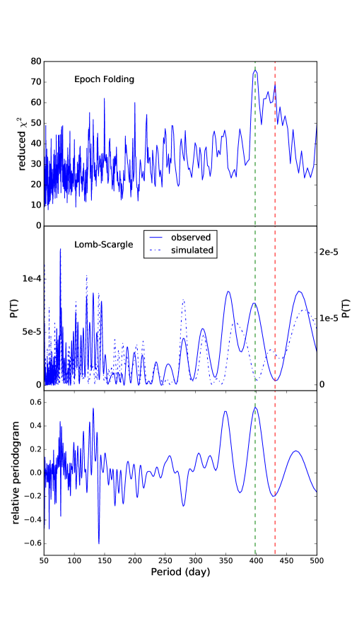
Figure 1: The period of SGR 1806-20 derived from sample A. This sample contains the observation of RXTE, which has over 3040 bursts. The top panel is the result of epoch-folding method. The Lomb-Scargle periodogram of observed data and simulated data are shown in the middle panel with blue solid line and blue dot-dashed line, respectively. The simulated data are uniformly distributed in the observation windows, so these peaks are caused by the observation windows. We normalized these two periodgrams with the maximum value and subtract the simulated periodogram from the observed one. The result is shown in the bottel panel with blue solid line. The green dashed line indicates the period derived from epoch-folding, which is 398.20 day. This period is consistent with a peak of Lomb-Scargle method. Considering the peak caused by the observation window, the maximum peak is also consistent with this period. The red dashed line is another peak in the reduce $\chi^{2}$, which is consistent with a peak of simulated points. Therefore, this peak is caused by the observation window.

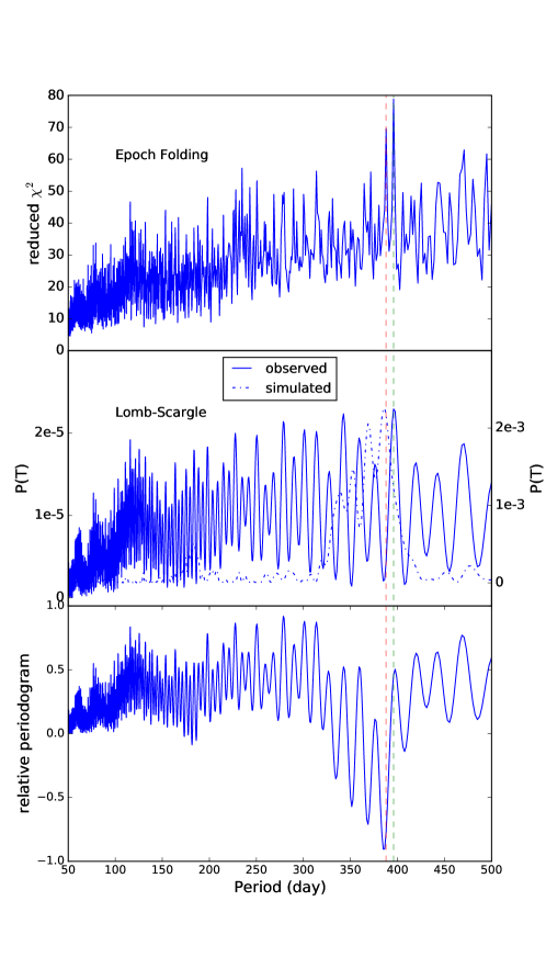
Figure 2: The period of SGR 1806-20 derived from sample B. This sample contains the observations of HETE-2, Konus and ICE. It contains 208 bursts. We show the results derived from epoch-folding and Lomb-Scargle periodogram. We show the reduce $\chi^{2}$ in the top panel. The vertical green line is the derived period 395.86 days. In the middle panel, the blue solid line is the observed periodogram and the blue dot-dashed line is the simulated periodogram. We normalized these two periodgrams with the maximum value and subtract the simulated periodogram from the observed one. The result is shown in the bottel panel. The green line indicates the best result of epoch-folding. It is consistent well with the period given by the Lomb-Scargle method. The vertical red dashed line is another significant peak of reduce $\chi^{2}$. This line is consistent with a peak of simulated periodogram, so it is caused by the observation window.

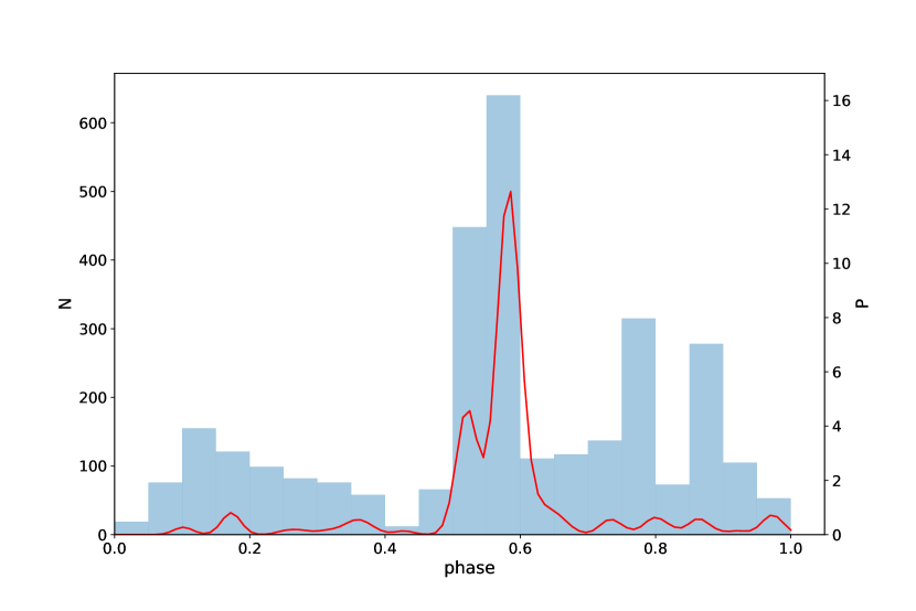
Figure 3: The folded phase of SGR 1806-20. The blue histogram is the distribution of sample A and the red line is the kernel density estimate of sample B. These two distributions are consistent with each other at the main peak $\psi\simeq 0.58$. In sample A, there are three minor peaks, which are invisible in sample B.

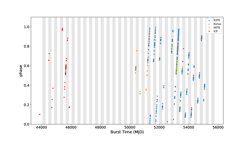
Figure 4: The MJD and phase of SGR 1806-20. The gray regions denote the main peak and the later two minor peaks in Figure 3. Due to the existence of other minor peaks, there are some points outside the gray regions.

References

- Alexander & Fedorova (2020) Alexander, R., & Fedorova, V. 2020, The Astronomer’s Telegram, 14186, 1
- Aptekar et al. (2001) Aptekar, R. L., Frederiks, D. D., Golenetskii, S. V., et al. 2001, ApJS, 137, 227, doi: 10.1086/322530
- Beloborodov (2017) Beloborodov, A. M. 2017, ApJ, 843, L26, doi: 10.3847/2041-8213/aa78f3
- Bochenek et al. (2020) Bochenek, C. D., Ravi, V., Belov, K. V., et al. 2020, arXiv e-prints, arXiv:2005.10828. https://arxiv.org/abs/2005.10828
- Cao et al. (2017) Cao, X.-F., Yu, Y.-W., & Dai, Z.-G. 2017, ApJ, 839, L20, doi: 10.3847/2041-8213/aa6af2
- Cheng et al. (2020) Cheng, Y., Zhang, G. Q., & Wang, F. Y. 2020, MNRAS, 491, 1498, doi: 10.1093/mnras/stz3085
- CHIME/FRB Collaboration et al. (2020) CHIME/FRB Collaboration, Amiri, M., Andersen, B. C., et al. 2020, Nature, 582, 351, doi: 10.1038/s41586-020-2398-2
- Cordes & Chatterjee (2019) Cordes, J. M., & Chatterjee, S. 2019, ARA&A, 57, 417, doi: 10.1146/annurev-astro-091918-104501
- Cruces et al. (2020) Cruces, M., Spitler, L. G., Scholz, P., et al. 2020, MNRAS, 500, 448, doi: 10.1093/mnras/staa3223
- Dai et al. (2016) Dai, Z. G., Wang, J. S., Wu, X. F., & Huang, Y. F. 2016, ApJ, 829, 27, doi: 10.3847/0004-637X/829/1/27
- Dai & Zhong (2020) Dai, Z. G., & Zhong, S. Q. 2020, ApJ, 895, L1, doi: 10.3847/2041-8213/ab8f2d
- Geng & Huang (2015) Geng, J. J., & Huang, Y. F. 2015, ApJ, 809, 24, doi: 10.1088/0004-637X/809/1/24
- Gourgouliatos et al. (2015) Gourgouliatos, K. N., Kondić, T., Lyutikov, M., & Hollerbach, R. 2015, MNRAS, 453, L93, doi: 10.1093/mnrasl/slv106
- Grossan (2020) Grossan, B. 2020, arXiv e-prints, arXiv:2006.16480. https://arxiv.org/abs/2006.16480
- Gu et al. (2020) Gu, W.-M., Yi, T., & Liu, T. 2020, MNRAS, 497, 1543, doi: 10.1093/mnras/staa1914
- Ioka & Zhang (2020) Ioka, K., & Zhang, B. 2020, ApJ, 893, L26, doi: 10.3847/2041-8213/ab83fb
- Israel et al. (2016) Israel, G. L., Esposito, P., Rea, N., et al. 2016, MNRAS, 457, 3448, doi: 10.1093/mnras/stw008
- Kaspi & Beloborodov (2017) Kaspi, V. M., & Beloborodov, A. M. 2017, ARA&A, 55, 261, doi: 10.1146/annurev-astro-081915-023329
- Katz (2016) Katz, J. I. 2016, ApJ, 826, 226, doi: 10.3847/0004-637X/826/2/226
- Kirsten et al. (2020) Kirsten, F., Snelders, M. P., Jenkins, M., et al. 2020, Nature Astronomy, doi: 10.1038/s41550-020-01246-3
- Kouveliotou et al. (1998) Kouveliotou, C., Dieters, S., Strohmayer, T., et al. 1998, Nature, 393, 235, doi: 10.1038/30410
- Kulkarni et al. (2014) Kulkarni, S. R., Ofek, E. O., Neill, J. D., Zheng, Z., & Juric, M. 2014, ApJ, 797, 70, doi: 10.1088/0004-637X/797/1/70
- Lander et al. (2015) Lander, S. K., Andersson, N., Antonopoulou, D., & Watts, A. L. 2015, MNRAS, 449, 2047, doi: 10.1093/mnras/stv432
- Laros et al. (1987) Laros, J. G., Fenimore, E. E., Klebesadel, R. W., et al. 1987, ApJ, 320, L111, doi: 10.1086/184985
- Levin et al. (2020) Levin, Y., Beloborodov, A. M., & Bransgrove, A. 2020, ApJ, 895, L30, doi: 10.3847/2041-8213/ab8c4c
- Li et al. (2020) Li, C. K., Lin, L., Xiong, S. L., et al. 2020, arXiv e-prints, arXiv:2005.11071. https://arxiv.org/abs/2005.11071
- Lin et al. (2020) Lin, L., Zhang, C. F., Wang, P., et al. 2020, Nature, 587, 63, doi: 10.1038/s41586-020-2839-y
- Lomb (1976) Lomb, N. R. 1976, Ap&SS, 39, 447, doi: 10.1007/BF00648343
- Lorimer et al. (2007) Lorimer, D. R., Bailes, M., McLaughlin, M. A., Narkevic, D. J., & Crawford, F. 2007, Science, 318, 777, doi: 10.1126/science.1147532
- Lyubarsky (2014) Lyubarsky, Y. 2014, MNRAS, 442, L9, doi: 10.1093/mnrasl/slu046
- Lyutikov et al. (2020) Lyutikov, M., Barkov, M. V., & Giannios, D. 2020, ApJ, 893, L39, doi: 10.3847/2041-8213/ab87a4
- Marcote et al. (2020) Marcote, B., Nimmo, K., Hessels, J. W. T., et al. 2020, Nature, 577, 190, doi: 10.1038/s41586-019-1866-z
- Mereghetti et al. (2020) Mereghetti, S., Savchenko, V., Ferrigno, C., et al. 2020, ApJ, 898, L29, doi: 10.3847/2041-8213/aba2cf
- Metzger et al. (2017) Metzger, B. D., Berger, E., & Margalit, B. 2017, ApJ, 841, 14, doi: 10.3847/1538-4357/aa633d
- Murase et al. (2016) Murase, K., Kashiyama, K., & Mészáros, P. 2016, MNRAS, 461, 1498, doi: 10.1093/mnras/stw1328
- Nakagawa et al. (2007) Nakagawa, Y. E., Yoshida, A., Hurley, K., et al. 2007, PASJ, 59, 653, doi: 10.1093/pasj/59.3.653
- Olausen & Kaspi (2014) Olausen, S. A., & Kaspi, V. M. 2014, ApJS, 212, 6, doi: 10.1088/0067-0049/212/1/6
- Palmer et al. (2005) Palmer, D. M., Barthelmy, S., Gehrels, N., et al. 2005, Nature, 434, 1107, doi: 10.1038/nature03525
- Petroff et al. (2019) Petroff, E., Hessels, J. W. T., & Lorimer, D. R. 2019, A&A Rev., 27, 4, doi: 10.1007/s00159-019-0116-6
- Platts et al. (2019) Platts, E., Weltman, A., Walters, A., et al. 2019, Phys. Rep., 821, 1, doi: 10.1016/j.physrep.2019.06.003
- Prieskorn & Kaaret (2012) Prieskorn, Z., & Kaaret, P. 2012, ApJ, 755, 1, doi: 10.1088/0004-637X/755/1/1
- Rajwade et al. (2020) Rajwade, K. M., Mickaliger, M. B., Stappers, B. W., et al. 2020, MNRAS, 495, 3551, doi: 10.1093/mnras/staa1237
- Scargle (1982) Scargle, J. D. 1982, ApJ, 263, 835, doi: 10.1086/160554
- Shaham (1977) Shaham, J. 1977, ApJ, 214, 251, doi: 10.1086/155249
- Sob’yanin (2020) Sob’yanin, D. N. 2020, MNRAS, 497, 1001, doi: 10.1093/mnras/staa1976
- Tendulkar et al. (2016) Tendulkar, S. P., Kaspi, V. M., & Patel, C. 2016, ApJ, 827, 59, doi: 10.3847/0004-637X/827/1/59
- The CHIME/FRB Collaboration et al. (2020) The CHIME/FRB Collaboration, :, Andersen, B. C., et al. 2020, arXiv e-prints, arXiv:2005.10324. https://arxiv.org/abs/2005.10324
- Thompson & Duncan (1995) Thompson, C., & Duncan, R. C. 1995, MNRAS, 275, 255, doi: 10.1093/mnras/275.2.255
- Tong et al. (2020) Tong, H., Wang, W., & Wang, H. G. 2020, arXiv e-prints, arXiv:2002.10265. https://arxiv.org/abs/2002.10265
- Ulmer et al. (1993) Ulmer, A., Fenimore, E. E., Epstein, R. I., et al. 1993, ApJ, 418, 395, doi: 10.1086/173399
- VanderPlas (2018) VanderPlas, J. T. 2018, ApJS, 236, 16, doi: 10.3847/1538-4365/aab766
- Wadiasingh & Timokhin (2019) Wadiasingh, Z., & Timokhin, A. 2019, ApJ, 879, 4, doi: 10.3847/1538-4357/ab2240
- Wang et al. (2020) Wang, F. Y., Wang, Y. Y., Yang, Y.-P., et al. 2020, ApJ, 891, 72, doi: 10.3847/1538-4357/ab74d0
- Wang & Yu (2017) Wang, F. Y., & Yu, H. 2017, J. Cosmology Astropart. Phys, 03, 023, doi: 10.1088/1475-7516/2017/03/023
- Woods et al. (2007) Woods, P. M., Kouveliotou, C., Finger, M. H., et al. 2007, ApJ, 654, 470, doi: 10.1086/507459
- Wu et al. (2020) Wu, Q., Zhang, G. Q., Wang, F. Y., & Dai, Z. G. 2020, arXiv e-prints, arXiv:2008.05635. https://arxiv.org/abs/2008.05635
- Xiao et al. (2021) Xiao, D., Wang, F., & Dai, Z. 2021, arXiv e-prints, arXiv:2101.04907. https://arxiv.org/abs/2101.04907
- Yang & Zou (2020) Yang, H., & Zou, Y.-C. 2020, ApJ, 893, L31, doi: 10.3847/2041-8213/ab800f
- Zanazzi & Lai (2020) Zanazzi, J. J., & Lai, D. 2020, ApJ, 892, L15, doi: 10.3847/2041-8213/ab7cdd
- Zhang (2017) Zhang, B. 2017, ApJ, 836, L32, doi: 10.3847/2041-8213/aa5ded
- Zhang (2018) —. 2018, ApJ, 854, L21, doi: 10.3847/2041-8213/aaadba
- Zhang (2020a) —. 2020a, Nature, 587, 45, doi: 10.1038/s41586-020-2828-1
- Zhang (2020b) —. 2020b, arXiv e-prints, arXiv:2011.09921. https://arxiv.org/abs/2011.09921
- Zhang et al. (2020) Zhang, C. F., Jiang, J. C., Men, Y. P., et al. 2020, The Astronomer’s Telegram, 13699, 1
- Zhao et al. (2020) Zhao, Z. Y., Zhang, G. Q., Wang, Y. Y., & Wang, F. Y. 2020, arXiv e-prints, arXiv:2010.10702. https://arxiv.org/abs/2010.10702