Sub-arcsecond Imaging of the Complex Organic Chemistry in Massive Star-forming Region G10.6-0.4

Abstract

Massive star-forming regions exhibit an extremely rich and diverse chemistry, which in principle provides a wealth of molecular probes, as well as laboratories for interstellar prebiotic chemistry. Since the chemical structure of these sources displays substantial spatial variation among species on small scales (${\lesssim}10^{4}$ au), high angular resolution observations are needed to connect chemical structures to local environments and inform astrochemical models of massive star formation. To address this, we present ALMA 1.3 mm observations toward OB cluster-forming region G10.6-0.4 (hereafter “G10.6”) at a resolution of 0.14^′′ (700 au). We find highly-structured emission from complex organic molecules (COMs) throughout the central 20,000 au, including two hot molecular cores and several shells or filaments. We present spatially-resolved rotational temperature and column density maps for a large sample of COMs and warm gas tracers. These maps reveal a range of gas substructure in both O- and N-bearing species. We identify several spatial correlations that can be explained by existing models of COM formation, including NH₂CHO/HNCO and CH₃OCHO/CH₃OCH₃, but also observe unexpected distributions and correlations which suggest that our current understanding of COM formation is far from complete. Importantly, complex chemistry is observed throughout G10.6, rather than being confined to hot cores. The COM composition appears to be different in the cores compared to the more extended structures, which illustrates the importance of high spatial resolution observations of molecular gas in elucidating the physical and chemical processes associated with massive star formation.

1 Introduction

Although high-mass stars (${>}8~{}M_{\odot}$) play a dominant role in cosmic evolution, chemical enrichment of the interstellar medium, galaxy formation and evolution, and galactic star formation, a detailed understanding of their formation remains elusive due to their short evolutionary timescales, intrinsic rarity, large distances, and heavy obscuration (Zinnecker & Yorke, 2007; Tan et al., 2014; Motte et al., 2018). A further complication arises due to the complex, multi-component process of forming massive protostars, which substantially alter their surroundings, as they become energetic enough to ionize their natal molecular clouds. This first produces hypercompact (HC) H II regions of sizes ${\sim}0.01$ pc (Kurtz et al., 2000), which then expand to form ultracompact (UC) H II regions of sizes ${\sim}0.1$ pc (Churchwell, 2002; Hoare et al., 2007), and ultimately with time, compact H II regions, before all of the material surrounding the newly-formed stars are destroyed or dispersed by powerful stellar winds. During this process, these regions possess an extremely rich and diverse chemistry, as the chemical composition of molecular gas involved in star formation is greatly influenced by the physical changes that occur during the star formation process (van Dishoeck & Blake, 1998).

In particular, the elevated temperatures and densities generated from collapsing material leads to the production and destruction of various molecular species and results in a high degree of chemical complexity (Schilke et al., 2001; Bisschop et al., 2007; Belloche et al., 2013), which in turn leads to the emergence of hot molecular cores. These hot cores, which exhibit intense emission in numerous complex organic molecules (COMs), are often associated with hot and dense regions near massive young stellar objects (MYSOs). However, the complex chemical and physical processes driving these regions are not fully understood, despite decades of observational (Blake et al., 1987; Gibb et al., 2000) and modeling efforts (Charnley et al., 1992, 1995a, 1995b; Garrod & Herbst, 2006; Garrod et al., 2008; Laas et al., 2011; Choudhury et al., 2015). For instance, the presence of externally-heated hot cores located in the vicinity of UC H II regions (Wyrowski et al., 1999; De Buizer et al., 2003; Mookerjea et al., 2007) has challenged the notion that hot cores are simply a stage in the evolutionary sequence of massive protostars. In reality, hot cores may also originate as chemical manifestations of UC H II regions on their environments, rather than simply being precursors to UC H II regions, and be driven, in part, by COM production from ice photochemistry due to abundant UV and X-ray photons (Öberg, 2016).

Numerous studies at low spatial resolution confirmed the presence of a COM-rich chemistry in MYSOs (e.g., Turner, 1991; Schilke et al., 1997; Tercero et al., 2010), while those conducted at higher resolution revealed that this chemistry is highly-structured on small scales ($\lesssim 10^{4}$ au) (e.g., Beuther et al., 2005; Mookerjea et al., 2007; Qin et al., 2010; Guzmán et al., 2018; Moscadelli et al., 2018; Bøgelund et al., 2019; Gieser et al., 2019; Molet et al., 2019). Such observations, which directly resolve the spatial differences between the emission of distinct species allow us to unambiguously discern the regions traced by different molecular species and families of molecules, providing further insight into their formation processes and chemistry. As a result, they are crucial for constraining a variety of outstanding questions related to the chemical evolution of MYSOs: How frequently and in what way are hot cores associated with UC H II regions (e.g., Mookerjea et al., 2007; Lindberg et al., 2017)? What processes and evolutionary stages are responsible for COM production in massive star-forming regions (e.g., Garrod et al., 2017; El-Abd et al., 2019)? Are there several distinct COM chemistries that can be used to trace different aspects of star formation (e.g., Fontani et al., 2007; Suzuki et al., 2018; Tercero et al., 2018)? Are O- and N-bearing COMs systematically spatially offset from one another (e.g., Blake et al., 1987; Wyrowski et al., 1999; Qin et al., 2010; Jiménez-Serra et al., 2012)?

To address these questions, we investigated the small-scale spatial structure of a representative set of COMs in the well-known massive star-forming region G10.6-0.4 (hereafter “G10.6”). G10.6 is a ${\sim}10^{6}~{}L_{\odot}$ OB cluster-forming region (Casoli et al., 1986; Lin et al., 2016) at a distance of 4.95 kpc (Sanna et al., 2014b). Unresolved observations with the Submillimeter Array (SMA) revealed that the dense gas surrounding its central proto-OB-cluster is particularly COM- and hydrocarbon-rich (Jiang et al., 2015; Wong & An, 2018). Hints of chemical substructure were seen in ${\sim}1^{\prime\prime}$ resolution SMA observations of a sample of shock tracer molecules, especially in E${}_{\rm{u}}\approx 100$–$150$ K lines of SO₂ and OCS (Liu et al., 2010b). These observations suggested a rich, spatially-variable complex chemistry taking place in the central $3^{\prime\prime}$ (${\sim}0.09$ pc).

In this paper, we present a detailed study of the complex chemistry toward the central 20,000 au of G10.6 using ALMA Band 6 observations at $0.14^{\prime\prime}$. In Section 2, we describe the observations and data reduction. In Section 3, we discuss the methods for extracting spatially-resolved gas physical conditions and show a detailed example for CH₃OH. We present rotational temperature and column density maps, as well as spatial correlations for all molecules in our sample in Section 4. We discuss the COM chemistry of G10.6 and compare it with other well-studied regions in Section 5 and summarize our conclusions in Section 6.

2 Observations

2.1 Observational Details

G10.6 was observed on 9-10 September 2016 and 19 July 2017 in Band 6 as part of the ALMA Cycle 5 project 2015.1.00106.S. The first execution block included 36 antennas with projected baseline lengths between 15 and 3144 m (11–2462 k$\lambda$). The second execution block included 41 antennas with projected baseline lengths between 15 and 3697 m (11–2896 k$\lambda$). The on-source integration times were 67 min and 66 min, respectively, for a total on-source integration time of 2.2 hr. Precipitable water vapor was 0.50 mm and 0.46 mm with system temperatures ranging between 54–75 K and 50–70 K for each execution block, respectively. The correlator setup was identical for both execution blocks and included spectral windows centered at 217.9, 220.0, 232.0, and 233.9 GHz with a uniform resolution of 976.563 kHz (${\sim}1.3$ km s^-1). Each spectral window had a bandwidth of 1.875 GHz for a total bandwidth of 7.5 GHz. The spectral setup was motivated by the primary science goal of studying the kinematics of the H$30\alpha$ hydrogen radio recombination line, which will be described in a future paper. The auxiliary molecular line data were obtained gratuitously, and for this reason, the dataset was not necessarily optimized for maximal coverage of COM lines.

The phase center of both observations was located at R.A. (J2000)$=$18^h10^m28^s.683, Dec. (J2000)$=$ $-$19^∘55^′49^′′.07. The full-width at half-maximum (FWHM) of the ALMA primary beam was 25.1^′′, and as a result, primary beam corrections were not necessary. For both executions, the quasar J1924-2914 was used for bandpass calibration and J1832-2039 was used for phase calibration, while J1733-1304 served as the flux calibrator. We assume a 10% flux calibration uncertainty.

2.2 Data Reduction, Continuum Subtraction, and Imaging

Initial data calibration was performed by ALMA / NAASC staff. The reduction of the first execution used CASA version 4.7.0, while the reduction of the second execution and all subsequent imaging used CASA version 4.7.2 (McMullin et al., 2007). The data cubes were imaged using the tclean task with a Briggs robust weighting parameter of 0.5 to achieve a compromise between resolution and sensitivity to extended emission. The resulting images have a square pixel size of $0.018^{\prime\prime}$ and an overall size of ${\sim}43^{\prime\prime}$, which is approximately twice the primary beam FWHM at 1.3 mm. We then trimmed these images to the innermost 9^′′ by 7^′′ region, which is known to contain the densest gas and hence the most complex and varied chemistry (e.g., Liu et al., 2010b).

Due to the high sensitivity and dynamic range of the observations, no sufficiently “line-free” channels exist across the entirety of the map, especially toward regions containing the densest gas. As a result, we were unable to subtract the continuum emission in the Fourier domain and instead performed the continuum subtraction in the image plane. We followed the procedures of Jørgensen et al. (2016) to define the continuum in a homogeneous and automated way based on the density distribution of channel intensities in each pixel. In brief, the flux density distribution of each pixel was first fit with a symmetric Gaussian. Then, the centroid of this fit was used to define a fitting range for a skewed Gaussian fit and the new centroid value (no longer necessarily symmetric) was recorded as the continuum level for that particular pixel. For pixels with only continuum contribution and no line emission, the distribution is a symmetric Gaussian centered at the continuum level with a width corresponding to the rms noise $\sigma$, while pixels with both continuum and line emission are modified by an exponential tail toward higher values. Jørgensen et al. (2016) report an accuracy of $2\sigma$ using this method, and as this study focuses on strong lines (${>}20\sigma$), the continuum subtraction contribution to our total error budget is minimal. The accuracy of our continuum subtraction was confirmed via visual inspection, and we did not find it necessary to implement more sophisticated continuum subtraction methods (e.g., Sánchez-Monge et al., 2018; Molet et al., 2019).

Table 1: Overview of Spectral Windows

[-.3cm]    Frequency Range	Beam Size	P. A.	rms
[GHz]	[${}^{\prime\prime}\times^{\prime\prime}$]	[∘]	[mJy beam-1]	[K]
216.948 – 218.823	$0.15\times 0.13$	118	0.60	0.79
219.053 – 220.928	$0.15\times 0.13$	110	0.65	0.84
231.054 – 232.929	$0.14\times 0.12$	115	0.63	0.85
232.949 – 234.824	$0.14\times 0.12$	120	0.65	0.87

We derived the continuum rms for each spectral window as the median value of all pixels without significant continuum emission. To do so, we excluded the central 0.06 pc region of G10.6, which possesses highly-structured continuum emission, and point source-like emission associated with an independent UC H II region located to the west. The derived continuum rms was then used to derive rms per spectral bin. Overall, we found a typical continuum rms of ${\sim}0.60$–$0.65$ mJy beam^-1 (${\sim}0.79$–$0.87$ K) with a synthesized beam size of $0.14^{\prime\prime}$, which corresponds to an approximate physical scale of 700 au at the distance of G10.6. A summary of beam sizes and rms values per spectral window is shown in Table 2.2. Fully reduced spectral cubes are publicly available and included in the supporting materials of this paper.

2.3 Overview of G10.6

G10.6 is a well-suited target for a study of complex chemistry at high spatial resolution. Several H II and UC H II regions are present across the central ${\sim}10$ pc area, which suggests that massive star formation is simultaneously occurring over the entire molecular cloud (Ho & Haschick, 1986; Sollins & Ho, 2005). G10.6 exhibits a centrally concentrated distribution of gas (Lin et al., 2016) with several approximately radially-aligned, 5–10 pc dense gas filaments, which connect to a central ${\sim}1$ pc-scale massive molecular clump (Liu et al., 2012; Liu, 2017). Higher angular resolution observations of dense molecular gas tracers revealed that some of these large-scale filaments are converging to a rotating, ${\sim}0.6$ pc-scale massive molecular envelope (Omodaka et al., 1992; Ho et al., 1994; Klaassen et al., 2009; Liu et al., 2010a, b, 2011). The massive proto-OB stars and associated UC H II region (Ho et al., 1986; Sollins et al., 2005) are deeply embedded in this rotationally-flattened (Guilloteau et al., 1988; Keto et al., 1987, 1988) envelope, where low density gas around the rotational axis has either been photoionized or dispersed by expanding ionized gas (Liu et al., 2010a, 2011). High excitation (E${}_{\rm{u}}~{}{\gtrsim}~{}100$ K) molecular lines trace a ${\sim}0.1$ pc “hot toroid” at the center of this massive molecular envelope (Liu et al., 2010a; Beltrán et al., 2011), which hosts the luminous proto-OB cluster. VLA observations of NH₃ (3,3) satellite hyperfine line absorption at $0.1^{\prime\prime}$ showed that the dense gas comprising the hot toroid is extremely clumpy (Sollins & Ho, 2005). Overall, the geometric configuration of the central ${\sim}1$ pc-scale massive molecular clump resembles that of a scaled-up version of a low-mass star-forming core and disk system viewed edge-on. For a more detailed, multi-scale view of G10.6 and its environment, see Liu (2017).

2.4 Observed Small-Scale Structure of G10.6

To better contextualize COM emission in the central region of G10.6, it is beneficial to first understand the broader physical conditions and gas structures as revealed by the continuum emission and distribution of ionized gas as shown in Figure 1. For consistency, we adopt the same nomenclature used in Sollins et al. (2005) and denote prominent features as A1–A6, B1–B5, C1–C2, and D. Features labeled as A correspond to localized arcs of ionized gas, and those marked as B are associated with a central cavity evacuated by a wide-angle outflow, as traced by strongly-emitted ionized gas. In particular, B1, B3, and B4 define the southwest edges of this outflow, while B2 and B5 mark the northeast edges. B5 is also the location of an elongated ridge containing the brightest H30$\alpha$ line emission and thus we also refer to it as the “ionized ridge”. Features labeled as C correspond to nearby but distinct H II regions. C1 (“C” in Sollins et al. (2005)) indicates a separate HC H II region located to the northwest, while C2 marks an independent UC H II region to west of the main H II region of G10.6. Feature D illustrates the presence of diffuse continuum and H30$\alpha$ line emission, which is present around the entire H II region except toward the evacuated outflow cavity. We also introduce the HC1–HC2 markings to indicate the locations of two newly-discovered hot molecular cores, which are characterized by compact continuum emission. HC1 is located along B4, making it coincident with the northwest outflow edge, while HC2 lies to the west of B5 and toward the periphery of the northeast edge of the ionized cavity.

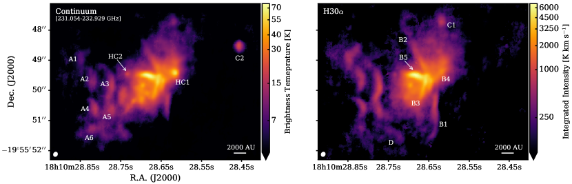
Figure 1: Overview of 1.3 mm continuum (left) and H30$\alpha$ line emission (right) in G10.6. Only S/N ${\geq}5\sigma$ continuum emission is shown. Prominent morphological features are labeled as A1–A6, B1–B6, C1–C2, D, and HC1–HC2. A log10 stretch is applied to the color scales of both panels to increase the visibility of substructures throughout G10.6. The synthesized beam is shown in the lower left of each panel.

Although more spatially-extended, the ionized gas largely traces the continuum emission, as expected, since the majority of the millimeter continuum originates from free-free emission (Liu et al., 2010b). However, we see a local maximum in continuum emission toward both HC1 and C2, but do not observe similar peaks in the H30$\alpha$ line, which indicates contributions from thermal dust emission. A similar but less pronounced effect is seen toward HC2. Interestingly, in the continuum map, we see diffuse material behind and between the ionized arcs traced by the H30$\alpha$ line emission, which implies that these structures are comprised of dusty neutral material whose surfaces are ionized. In fact, the H30$\alpha$ line map is more morphologically similar to the VLA 1.3 cm continuum presented in Sollins et al. (2005) than to the 230 GHz continuum.

3 Data Analysis

3.1 Molecule Sample

The ALMA observations of G10.6 cover a wide bandwidth, which provides coverage of numerous rotational transitions of many molecular species. We selected a chemically representative set of COMs commonly observed toward massive star-forming regions. These molecules are: CH₃OH, CH₃OCH₃, CH₃OCHO, CH₃CHO, NH₂CHO, CH₃CH₂CN, CH₂CHCN, CH₃CN, and HNCO. We also included the isotopologues ¹³CH₃CN, CH${}_{3}^{13}$CN, and ¹³CH₃OH, which not only provide valuable information about isotopic abundances in G10.6, but also trace denser and more optically thin gas relative to their main species. Each species had a sufficient number of lines to robustly derive rotational and column densities via a population diagram method over a wide spatial area in G10.6. Table 3.1 summarizes the number of identified lines, range of upper state energies, and Einstein A coefficients covered by these lines. An example of the analysis process is shown for CH₃OH in the following subsections.

Table 2: Summary of Targeted Species

[-.3cm]    Species	Name	Nlines	Eu	Aul	Catalog	Fitting Threshold
			[K]	$\times 10^{-5}$ [s-1]		Nlines	$\Delta$Eu [K]
CH3OH	Methanol	10	46 – 802	2.04 – 4.69	CDMS	3	51
13CH3OH		5	48 – 594	1.30 – 5.27	CDMS	3	206
CH3OCH3	Dimethyl Ether	7	81 – 673	1.44 – 9.14	CDMS	3	57
CH3OCHO	Methyl Formate	31	100 – 282	3.42 – 18.39	JPL	5	100
CH3CHO	Acetaldehyde	11	82 – 183	28.84 – 44.45	JPL	4	50
NH2CHO	Formamide	10	61 – 175	74.75 – 147.23	CDMS	9	114
CH3CN	Methyl Cyanide	11	69 – 931	10.10 – 63.71	JPL	7	257
13CH3CN		10	78 – 942	30.45 – 107.96	JPL	8	350
CH${}_{3}^{13}$CN		8	69 – 419	60.71 – 92.31	JPL	6	179
CH3CH2CN	Ethyl Cyanide	31	33 – 837	3.04 – 105.49	CDMS	18	172
CH2CHCN	Vinyl Cyanide	12	135 – 435	216.94 – 321.65	CDMS	5	25
HNCO	Isocyanic Acid	10	58 – 1050	6.68 – 24.02	CDMS	3	170

To illustrate the chemical and physical diversity across G10.6, Figure 2 shows integrated intensity maps for representative lines with comparable excitation conditions (E${}_{\rm{u}}\approx 100$ K) from each COM in our sample. We also extracted spectra from representative positions labeled in Figures 1 and 2. Spectra covering half of the observed bandwidth are shown in Figure 3, while the other half are shown in Figure A20 in Appendix A. Key lines are labeled, but we did not attempt a detailed identification of all lines within the spectral coverage and instead focus on those originating from the selected COMs. A high degree of variation in line strength, width, and richness is evident. Some COMs, e.g., NH₂CHO and CH₂CHCN, are seen primarily toward HC1, while other COMs, such as CH₃CN and CH₃OH, are observed in almost all positions, albeit at varying intensity levels.

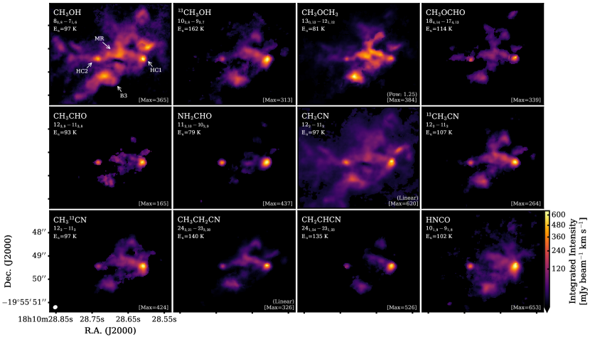
Figure 2: Integrated intensity maps for transitions with E${}_{\rm{u}}\approx 100$ K for all molecules in our sample. A square root stretch, unless otherwise indicated, is applied to each panel to better illustrate line substructure. The peak integrated line intensity is shown in the lower right of each panel.

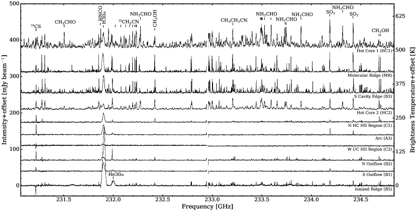
Figure 3: Spectra extracted from single pixels toward ten representative positions across the central 20,000 au of G10.6. Dashed lines represent gaps in observational coverage between spectral windows.

3.2 Fitting Process

For each species in the selected COM sample, we identified and fit all unblended transitions with single Gaussian profiles. All lines belonging to a single species were fit consistently. Blended lines were removed via visual inspection, while line assignments were checked by verifying that the best-fit model for each species did not predict lines at frequencies, covered by our observations, where no emission is detected.

In order to verify the spatial consistency of the spectral fits, we also visually inspected integrated intensity, systemic velocity, and line FWHM maps for each transition included in our analysis. In all cases, we found a reasonably coherent and smoothly-varying morphology throughout G10.6 (see Appendix B). We also confirmed that, in each case, the distribution of velocity and line FWHM values were not sharply peaked toward either the minimum or maximum limits designated in the fitting code. A representative set of maps are shown in Figure 4 for CH₃OH.

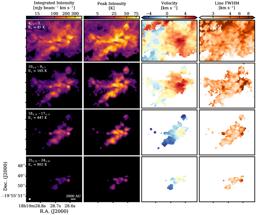
Figure 4: Integrated intensity, peak intensity, systemic velocity, and line FWHM (columns from left to right) are shown for four CH₃OH transitions spanning 45–802 K in E_u toward G10.6. Peak line intensity maps are included, as it is often easier to identify spatial trends across wide dynamic ranges. Each column shares the same color scale. To highlight gas substructure, a square root stretch is applied to the integrated and peak intensity maps, while an arcsinh stretch is used for the line FWHM map.

We then constructed maps of rotational temperature and column density for each COM species using a rotational diagram analysis (e.g., Goldsmith & Langer, 1999) on a pixel-by-pixel basis. To ensure secure determinations of rotational temperature and column density across a large spatial extent in G10.6, we restricted our fittings to those pixels with a sufficient number of lines with a wide coverage of E_u, as shown in Table 3.1.

We used the Markov Chain Monte Carlo (MCMC) code emcee (Foreman-Mackey et al., 2013) to generate posterior probability distributions of column densities and rotational temperatures consistent with the observed data. Random draws from these posteriors are plotted in purple for several positions toward G10.6 in Figure 5 with $\tau$-corrected values of N${}_{\rm{u}}/$g_u plotted against E_u. The derived parameters and uncertainties are listed as the 50th, 16th, and 84th percentiles from the marginalized posterior distributions, respectively.

In general, we initially explored a parameter space from $10^{14}$ cm${}^{-2}\leq$ N${}_{\rm{col}}\leq 10^{20}$ cm^-2 and 10 K $\leq$ T${}_{\rm{rot}}\leq 800$ K, based on physical gas conditions expected in massive star-forming regions (Bisschop et al., 2007; Suzuki et al., 2018; Molet et al., 2019). After this first model run, we ran a second iteration with narrower, species-specific grids and then performed quality checks to ensure that the fitted T_rot and N_col values were not sharply peaked at the extremes of our priors. For each line and species, we also visually inspected the fitted $\tau$ values across G10.6 and ensured that $\tau$ was spatially well-behaved and that $\tau\not\gg 1$. Optically-thick lines were excluded from the rotational diagram analysis. A detailed discussion of the line fitting process and rotational temperature and column density determination is presented in Appendix C.

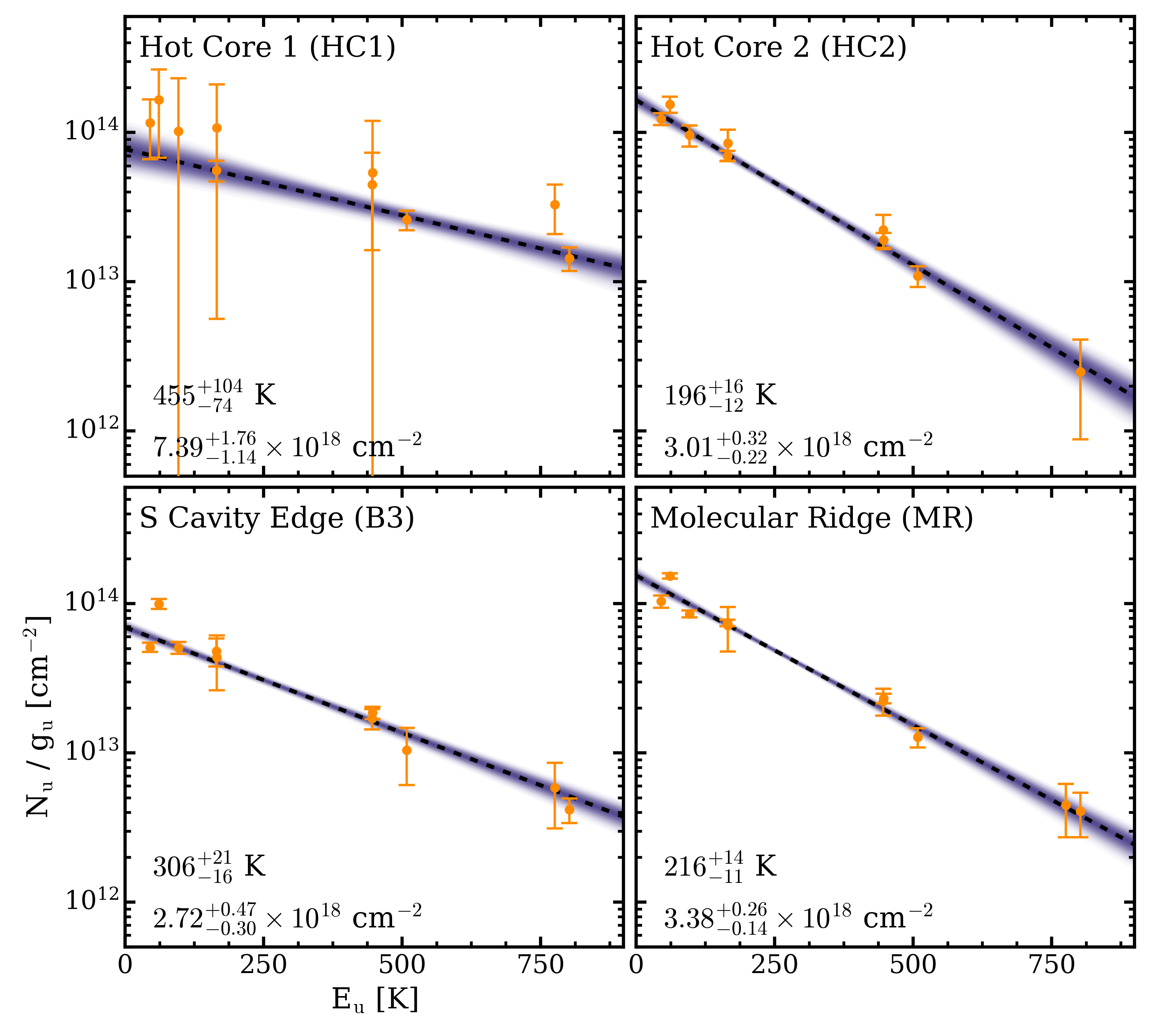
Figure 5: CH₃OH rotational diagrams toward positions of interest in G10.6. Transitions are shown in orange and random draws from the fit posteriors are plotted in purple. The fit is indicated by a dashed, black line and the derived values are shown in the lower left corners.

The resultant rotational temperature and column density maps derived for CH₃OH are shown in Figure 6. As a result of this MCMC fitting process, we also derived formal temperature and column density uncertainties, which were found to be low toward the central region of G10.6, but became large toward the edges of the map. This is not unexpected as we detect fewer high E_u lines toward the edges of the map and the lines that we do detect decrease in intensity relative to those toward the central region of G10.6, which increases the Gaussian fitting errors. A similar trend was found in all of the molecules in our sample and in no cases did we observe large spatial regions of unexpectedly high uncertainties. In addition to the initial quality cuts shown in Table 3.1, we also excluded pixels with particularly high uncertainties (${>}200\%$) and those with highly discontinuous and outlier values. Thus, a lack of model result for a specific pixel does not necessarily imply the absence of molecular emission, as is clearly seen when comparing integrated line intensities (Figure 2) and column density maps (Figure 9) for several species.

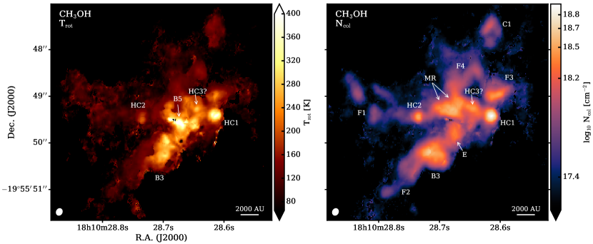
Figure 6: Rotational temperature (left) and column density (right) maps for CH₃OH. Prominent gas substructures are labeled as HC1-3, MR, E, and F1-4, in addition to the nomenclature from Sollins et al. (2005) used in Figure 1. An arcsinh stretch is applied to the color scale of the column density map to increase the visibility of substructures throughout G10.6. The synthesized beam is shown in the lower left of each panel.

Column densities and rotational temperature maps were derived using the method above with no modifications for six out of nine species in our sample. However, three molecules warranted special treatment: CH₃OCHO, CH₃CH₂CN, and CH₃CN. We ware unable to derive independent rotational temperatures for CH₃OCHO, which exhibited unusually large scatter in its rotational diagrams, and instead adopted those of the chemically-similar molecule CH₃OH (e.g., Garrod & Herbst, 2006; Garrod et al., 2008) to derive column density. A two component rotational diagram was required to fit the majority of CH₃CH₂CN emission and regions of optically thick CH₃CN emission required the use of optically thin isotope CH${}_{3}^{13}$CN. These latter two cases are discussed in more detail in the following two subsections.

3.3 Two CH₃CH₂CN Temperature Components

All line data were further analyzed to explore whether the data were better fit by two distinct temperature components rather than a single component. A two-component fit was only favored for CH₃CH₂CN, in which we clearly identified two separate temperature components throughout most of G10.6. Wherever two components were needed, most of the column density is carried by the colder component, which we therefore designate as the primary component. To not overfit the data, we restricted this two-component analysis to instances where the secondary component had a rotational temperature that was $1.5\times$ in excess of that of the primary component. Otherwise, we fit that pixel with a single rotational temperature. We defined the total column density of CH₃CH₂CN as the sum of both components and used the total column density for all subsequent analysis. Previous indications of multiple CH₃CH₂CN temperature components were seen toward Orion KL by Daly et al. (2013), who also observed a similar transition between different components at E${}_{\rm{u}}\approx$150–200 K.

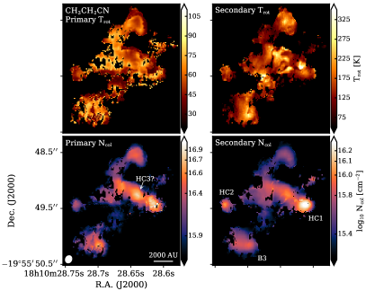
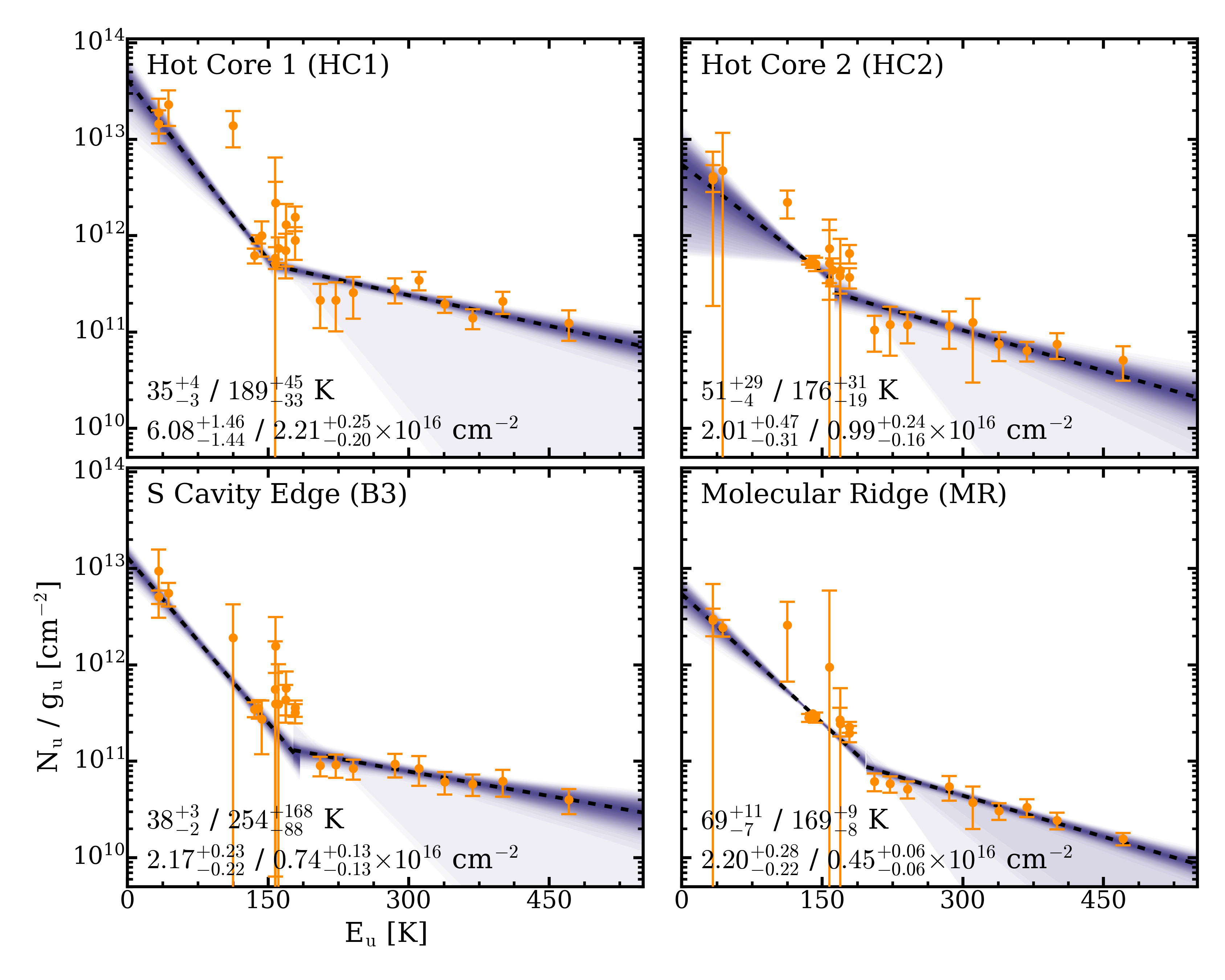
Figure 7: Two-component rotational diagram analysis for CH₃CH₂CN. Left four panels: Primary and secondary rotational temperature and column density maps. Right four panels: Representative rotational diagrams showing two-component fits toward regions of interest in G10.6.

3.4 Optically Thick CH₃CN and Isotopologues

Initial efforts to fit the central regions of CH₃CN revealed optically thick gas, as indicated by poor fittings and unphysical temperatures (T${}_{\rm{rot}}\gtrsim 1000$ K). High line optical depths ($\tau\sim 0.5$–$1.0$) were also observed in the 13–12 K-ladder of the ¹³CH₃CN isotopologue with the K=0–3 lines having $\tau\gtrsim 1$. However, the 12–11 K-ladder of CH${}_{3}^{13}$CN was found to be optically thin ($\tau<0.1$), allowing for secure rotational temperature and column density determinations. This approach requires a ¹²C/¹³C scaling factor, however, which is not known for CH₃CN in G10.6.

To derive this factor, we determined the ¹²C/¹³C ratio from the column density ratios of CH₃OH/¹³CH₃OH. A detailed discussion of this process is provided Appendix D. Overall, we find a median column density ratio of 22.8, which is the value we adopt. This is a factor of two lower than the expected ratio of 43 (Milam et al., 2005) at the distance of G10.6 (D${}_{\rm{GC}}=3.9$ kpc), but similar low values of ¹²C/¹³C have been derived in COMs at core scales in star-forming regions, e.g., hot corinos (Jørgensen et al., 2016) and hot cores (Sanna et al., 2014a; Beltrán et al., 2018; Bøgelund et al., 2019). However, the carbon isotopic ratio in G10.6 needs to be revisited with more comprehensive isotopologue data and as a result, the reported CH₃CN column densities in high density regions should only be considered accurate within a factor of 2.

4 Results

4.1 CH₃OH Substructure

COMs exhibit complex emission morphologies and substantial gas substructures across G10.6. As shown in Figure 6, this is well-illustrated by the rotational temperature and column density maps of CH₃OH, the most spatially-extended map in our sample. When appropriate, we refer to COM features, namely B3-5, C1, and HC1-2, using the nomenclature introduced above. For instance, hot cores HC1 and HC2 are clearly identified by their compact, high column densities and elevated temperatures. The south cavity edge (B3) contains a spatially-extended region of hot, high density gas, while the northeast cavity edge (B5) exhibits the hottest gas (${\gtrsim}400$ K) anywhere in G10.6 and possesses a relative deficit of molecular gas. Since B5 is also the location of an ionized ridge of material containing the brightest H30$\alpha$ line emission in G10.6, the hot, low column density gas associated with B5 may be the result of ionized gas heating and ultimately destroying some of surrounding molecular gas. The C1 region, which appeared compact and symmetric in continuum and ionized gas, is instead highly-structured in molecular gas and based on its arrow-shaped morphology, appears to be a cometary HC H II region (e.g., Wood & Churchwell, 1989).

Newly-identified gas substructures which have no obvious correspondence to the Sollins et al. (2005) features, are labeled as E, F1-F4, and MR. Feature E denotes a clump of gas within the central cavity of G10.6 and is bounded by the cavity edges B3 and B5. Four separate filamentary structures are marked as F. F1 is a tri-pronged structure on the eastern edge of G10.6, while F2 is comprised of a single narrow filament extending beyond B3. The F3 filament lies directly to the north of HC1 and may be related to hot core activity or may be simply a further extension of the “V”-shaped F4 filament located to the north of the MR. An elongated and somewhat irregular “Z”-shaped structure is seen immediately to the north of B5. As it is readily identified by a band of high density gas, we thus refer to this structure as the “molecular ridge,” denoting it as MR. The shape of the MR suggests that it is interacting with the ionized gas in B5 and its relative molecular richness (e.g., Figure 3) and high column density may be attributed to external heating from B5. The western portion of the MR appears to be marginally resolved into a core-like structure, which is tentatively labeled as HC3.

4.2 Rotational Temperatures and Column Densities

Spatially-resolved rotational temperature and column density maps for all molecules in our sample are shown in Figures 8 and 9, respectively. In terms of spatial coverage, NH₂CHO and CH₂CHCN are the most limited, CH₃OH and CH₃CN are the most extended, and the remaining species have intermediate spatial distributions. HC1 is prominent in all species, exhibiting elevated rotational temperatures and high column densities. HC2 is also seen in all column density maps, but is less enhanced in rotational temperature (except for HNCO). The MR and B3 also consistently exhibit high column densities in the majority of COMs. Filamentary features are seen in most molecules, although with varying extents and column densities. For instance, CH₃OCH₃ and CH₃OCHO show narrow features, e.g., F1 and F4, while CH₃CN is the only species with extended substructure comparable to that of CH₃OH. Interestingly, HC3 is consistently marginally resolved (e.g., CH₃OCHO, CH₃CN, CH₃CH₂CN), indicating the potential presence of high density clumps/cores that are unresolved in our observations.

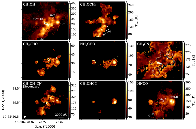
Figure 8: Rotational temperature maps for all species in our sample. The secondary temperature component of CH₃CH₂CN is shown. The white contours in CH₃CN indicate the regions where rotational temperatures were derived using the CH${}_{3}^{13}$CN isotopologue, as detailed in the text.

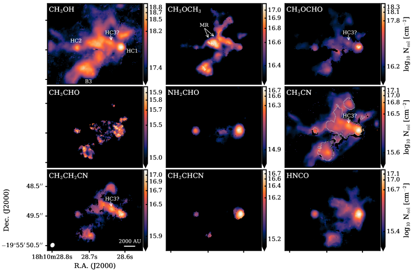
Figure 9: Column density maps for all species in our sample. The patchy nature of the CH₃CHO is due to higher fitting uncertainties, rather than true small-scale variations. The total column density, primary plus secondary components, is shown for CH₃CH₂CN. The white contours in CH₃CN indicate the regions where column densities were derived using the CH${}_{3}^{13}$CN isotopologue, as detailed in the text. An arcsinh stretch is applied to the color scales of all panels to increase the visibility of substructures throughout G10.6.

The rotational temperature maps reveal that there is no single temperature that characterizes all COMs at a specific location. Differences in temperatures span 100s of K, indicating that multiple environments are traced along the line of sight in this complex region. On average, CH₃CHO exhibits the lowest rotational temperatures (${\lesssim}60$ K), while NH₂CHO and CH₂CHCN have moderate temperatures (${\sim}70$–$150$ K). CH₃CN, CH₃OH, CH₃OCH₃, CH₃CH₂CN, and HNCO all possess substantially warmer temperatures (${\sim}$150–400 K).

Within the N-bearing COM family, we notice prominent differences between the spatial distributions of complex cyanides (CH₃CN, CH₃CH₂CN, CH₂CHCN) and HNCO. HNCO also displays a different temperature pattern, including a dual-peaked hot core 1 (HC1-D), a prominent HC2, and curved bands of elevated temperatures, which are marked as G in Figure 8. Together, these distinct column density and temperature patterns suggest that there is no single N-bearing COM chemistry and that the amount of nitrogen incorporated into different kinds of organics strongly depends on the local environment.

Among O-bearing species, CH₃OH, CH₃OCH₃, and CH₃OCHO each trace different structures in G10.6. CH₃OH is widely distributed throughout G10.6, as described in Section 4.1, while CH₃OCHO exhibits a significant enhancement in HC1 and shares broad morphological similarities with CH₃CHO, notwithstanding its increased uncertainties as reflected in a less uniform column density map. CH₃OCH₃ has an inverted “C”-shaped distribution of hot, clumpy gas (labeled as G) that connects the western edge of the MR to B3 and presents its highest column density in the MR rather than in HC1. This temperature and column density distribution is not seen in any other molecule in our sample, and may reflect the fact that CH₃OCH₃ is responding differently to strong radiation fields from nearby B5 than the other O-bearing COMs. By contrast, CH₃OH only shows weak enhancements along the MR, and CH₃OCHO shows none at all. Notably, the CH₃OCH₃ and CH₃OCHO maps appear strikingly different, which is somewhat surprising considering that all proposed chemical formation routes (e.g., Garrod & Herbst, 2006) indicate that they are directly linked.

Table 3: COM Rotational Temperatures and Column Densities at Regions of Interest in G10.6

[-.3cm]	Trot	NX	N${}_{\rm{X}/\rm{CH}_{3}\rm{OH}}$		Trot	NX	N${}_{\rm{X}/\rm{CH}_{3}\rm{OH}}$
	[K]	[$10^{16}$ cm-2]	[%]		[K]	[$10^{16}$ cm-2]	[%]
Hot Core 1 (HC1)				Hot Core 2 (HC2)
CH3OH	$455^{104}_{74}$	$739^{176}_{114}$	$100$	CH3OH	$196^{16}_{12}$	$301^{32}_{22}$	$100$
CH3OCH3	$147^{51}_{55}$	$5.51^{2.95}_{1.38}$	$0.75$	CH3OCH3	$101^{68}_{75}$	$3.51^{1.82}_{1.03}$	$1.2$
CH3OCHO	$\mathit{455^{104}_{74}}$	$259^{216}_{141}$	$35$	CH3OCHO	$\mathit{196^{16}_{12}}$	$12.0^{7.5}_{7.1}$	$4.0$
CH3CHO	$49^{38}_{20}$	$0.397^{0.026}_{0.024}$	$0.054$	CH3CHO	$24^{13}_{5}$	$0.625^{0.032}_{0.036}$	$0.21$
NH2CHO	$130^{2}_{2}$	$4.23^{0.36}_{0.33}$	$0.57$	NH2CHO	$63^{7}_{4}$	$1.27^{0.22}_{0.18}$	$0.42$
CH3CN	$\mathit{201^{79}_{47}}$	$14.8^{5.02}_{2.74}$	$2.0$	CH3CN	$\mathit{131^{42}_{17}}$	$3.65^{0.821}_{0.479}$	$1.2$
CH${}_{3}^{13}$CN	$201^{79}_{47}$	$0.654^{0.218}_{0.119}$	$0.088$	CH${}_{3}^{13}$CN	$131^{42}_{17}$	$0.164^{0.036}_{0.021}$	$0.054$
CH3CH2CN:	…	$8.29^{1.48}_{1.45}$	$1.1$	CH3CH2CN:	…	$3.00^{0.53}_{0.35}$	$1.0$
Primary	$35^{4}_{3}$	$6.08^{1.46}_{1.44}$	$0.82$	Primary	$51^{29}_{4}$	$2.01^{0.47}_{0.31}$	$0.67$
Secondary	$189^{45}_{33}$	$2.21^{0.25}_{0.20}$	$0.30$	Secondary	$176^{31}_{19}$	$0.99^{0.24}_{0.16}$	$0.33$
CH2CHCN	$139^{41}_{15}$	$6.19^{0.73}_{0.55}$	$0.84$	CH2CHCN	$84^{41}_{15}$	$0.747^{0.058}_{0.053}$	$0.25$
HNCO	$237^{42}_{27}$	$14.1^{6.6}_{1.8}$	$1.9$	HNCO	$166^{22}_{19}$	$2.72^{0.25}_{0.22}$	$0.90$
S Cavity Edge (B3)				Molecular Ridge (MR)
CH3OH	$306^{21}_{16}$	$272^{47}_{30}$	$100$	CH3OH	$216^{14}_{11}$	$338^{26}_{14}$	$100$
CH3OCH3	$179^{30}_{32}$	$6.94^{2.65}_{1.57}$	$2.6$	CH3OCH3	$179^{25}_{28}$	$9.06^{2.47}_{1.39}$	$2.7$
CH3OCHO	$\mathit{306^{21}_{16}}$	$16.0^{19.6}_{8.9}$	$5.9$	CH3OCHO	$\mathit{216^{14}_{11}}$	$5.28^{3.83}_{3.42}$	$1.6$
CH3CHO	$36^{13}_{5}$	$0.218^{0.032}_{0.036}$	$0.080$	CH3CHO	$24^{51}_{13}$	$0.263^{0.027}_{0.024}$	$0.078$
NH2CHO	$\mathit{135^{15}_{14}}$	${<}0.0102$	${<}0.0038$	NH2CHO	$\mathit{78^{26}_{23}}$	${<}0.0101$	${<}0.0030$
CH3CN	$\mathit{203^{42}_{17}}$	$4.77^{0.821}_{0.479}$	$1.8$	CH3CN	$\mathit{116^{13}_{11}}$	$2.51^{0.27}_{0.25}$	$0.74$
CH${}_{3}^{13}$CN	$203^{42}_{17}$	$0.209^{0.36}_{0.21}$	$0.077$	CH${}_{3}^{13}$CN	$116^{13}_{11}$	$0.110^{0.012}_{0.011}$	$0.033$
CH3CH2CN:	…	$2.91^{0.26}_{0.26}$	$1.1$	CH3CH2CN:	…	$2.65^{0.29}_{0.23}$	$0.79$
Primary	$38^{3}_{2}$	$2.17^{0.23}_{0.22}$	$0.80$	Primary	$69^{11}_{7}$	$2.20^{0.28}_{0.22}$	$0.65$
Secondary	$254^{168}_{88}$	$0.74^{0.13}_{0.13}$	$0.27$	Secondary	$169^{9}_{8}$	$0.45^{0.06}_{0.06}$	$0.13$
CH2CHCN	$67^{2}_{2}$	$0.973^{0.173}_{0.180}$	$0.36$	CH2CHCN	$\mathit{69^{11}_{7}}$	${<}0.0138$	${<}0.0041$
HNCO	$135^{15}_{14}$	$1.18^{0.14}_{0.14}$	$0.43$	HNCO	$78^{27}_{24}$	$0.160^{0.043}_{0.032}$	$0.047$

Note. — Uncertainties at the 1$\sigma$ level are reported. T_rot values in italics are those adopted from similar species, as described in the text. Column density upper limits are derived using $3\sigma$ line intensity upper limits and by assuming the median line FWHM from a chemically-related or observationally-linked species (e.g., CH₃CH₂CN/CH₂CHCN, HNCO/NH₂CHO; Caselli et al., 1993; Allen et al., 2020)

In Table 4.2, we provide a list of rotational temperature and column densities toward four regions of particular interest: HC1-2, B3, and MR. Figure 10 presents a summary of derived column densities toward these same positions. Column density variations between species span three orders of magnitude at each position, with CH₃OH being most abundant at all locations. HC1, HC2, and B3 appear broadly similar in their chemical compositions, as indicated by a similar distribution of COM abundances with respect to CH₃OH. However, HC1 exhibits at least an order of magnitude enhancement in CH₃OCHO relative to the other positions, while B3 is deficient in NH₂CHO and the MR is deficient in both NH₂CHO and CH₂CHCN.

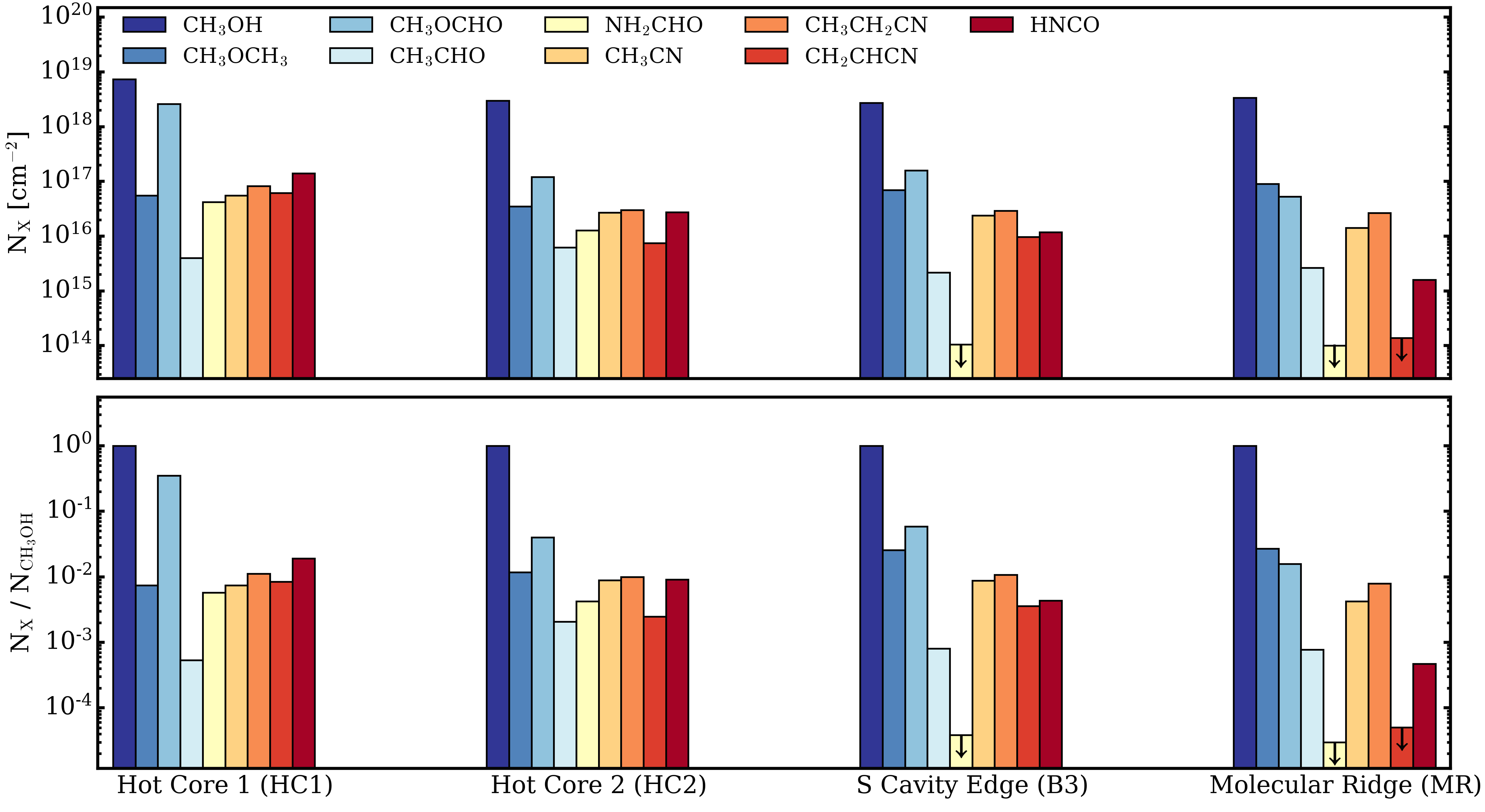
Figure 10: Histogram of absolute (top) and CH₃OH-normalized (bottom) column densities toward positions of interest in G10.6. Upper limits are indicated by downward arrows.

4.3 Spatial Column Density Correlations

To accurately compare spatial trends of different species, we first performed 1/4-beam sampling, i.e., 4 data points extracted for each beam area, on a consistent spatial grid that was then applied uniformly to all COMs in the sample and used for all subsequent correlation analysis. We did not attempt to derive fractional abundances with respect to hydrogen due to a lack of H₂ gas tracers on these scales; we cannot, for example, distinguish the free-free and dust contributions to the overall continuum emission. We instead compared column densities using the cross correlation between each pair of molecules according to Guzmán et al. (2018) via:

$$\rho_{12}=\dfrac{\displaystyle\sum_{i,j}I_{1,ij}I_{2,ij}w_{ij}}{\left(\displaystyle\sum_{i,j}I^{2}_{1,ij}w_{ij}\displaystyle\sum_{i,j}I^{2}_{2,ij}w_{ij}\right)^{1/2}}.$$ (1)

Sums were taken over each quarter beam position with $I_{1,ij}$ and $I_{2,ij}$ corresponding to the values at each position $i,j$ and the weight $w_{ij}$ is equal to either 0 or 1 if a column density was able to be determined for that position or not. By definition, $\rho_{12}=\rho_{21}$ and $|\rho_{12}|\leq 1$, and a value of $\rho_{12}=1$ implies that $I_{1}=\alpha I_{2}$, where $\alpha$ is a positive constant. Hence, the closer the cross correlation values are to 1, the more similar the spatial distributions of column density.

The left panel of Figure 11 shows the calculated cross correlations for all pairs of molecules, excluding CH₂CHCN, which lacked a sufficient number of independent data points for meaningful comparison. Although spatially compact, the column density map of NH₂CHO still covers nearly 20 independent beams and thus we chose to include it in this analysis. We find strong correlations between: NH₂CHO/HNCO and NH₂CHO/CH₃OCHO, which are dominated by HC1 and HC2; CH₃CN/CH₃CH₂CN and CH₃OH/CH₃OCH₃, which are expected to be chemically related and trace similar column density structures; and CH₃OH/CH₃CN, which are the two most extended molecules and likely probe total gas column densities. We also note that correlations between the saturated cyanides CH₃CH₂CN and CH₃CN are greater than those between pairs of saturated and unsaturated N-bearing species, such as CH₃CN/NH₂CHO, CH₃CH₂CN/NH₂CHO, or CH₃CH₂CN/HNCO. The weakest correlations are typically found between CH₃OCH₃ and molecules such as HNCO, NH₂CHO, and CH₃OCHO, which reflects the unique column density distribution of CH₃OCH₃.

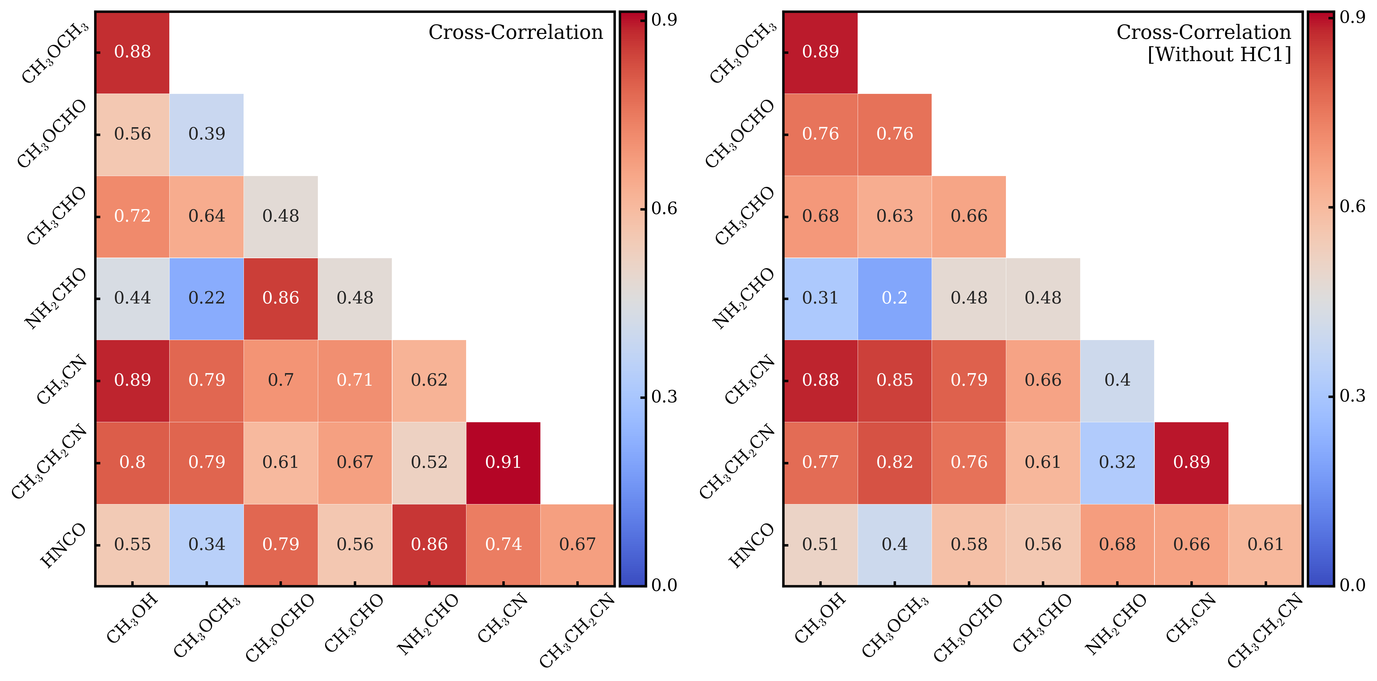
Figure 11: Column density correlation matrix, showing cross correlations with (left) and without HC1 (right) for each pair of molecules.

As noted by Guzmán et al. (2018), higher column density sections of an image weigh more into the calculation of $\rho_{12}$. In our case, HC1 possesses the highest column density for each species, except CH₃OCH₃. In order to avoid HC1 dominating the derived correlation coefficient and to search for additional spatial trends, we masked the pixels in a 0.16^′′ region centered on HC1. This masking region was chosen to be slightly larger than the average beam size, such that we fully excluded HC1, which is marginally-resolved in our observations. The resulting cross correlations are shown in the right panel of Figure 11.

As expected, correlations between NH₂CHO and HNCO and other species dramatically decrease, since these molecules are most prominently detected toward HC1. We do note, however, the caveat that only ${\sim}$10 independent beams are available for correlations involving NH₂CHO, which is a reduction of 50% after excluding HC1. Cross correlations involving the spatially-extended molecules CH₃OH and CH₃CN are roughly the same. CH₃OCH₃, despite its unique column density distribution, remains strongly correlated with CH₃OH irrespective of the inclusion or exclusion of HC1. We find that CH₃OCHO is now well-correlated with the other O-bearing COMs CH₃OH and CH₃OCH₃. This suggests that outside of HC1 these molecules co-form and that the hot core environment acts to specifically enhance or destroy some COMs that are otherwise chemically-related.

While cross correlations are informative of general chemical relatedness, they do not capture the fact that multiple trends within single molecular pairs may exist in G10.6. To investigate the existence of such correlations directly, we show correlation plots for each pair of molecules in Figure 12. We labeled the percentage overlap between the two molecules being compared in the upper left corner of each panel, which helps inform the spatial extent over which these trends can be reliably interpreted. We defined this percentage overlap as the fraction of pixels from the species with a smaller spatial extent relative to the fraction of pixels from the species with a larger spatial extent. For instance, the 54% overlap between CH₃OH and CH₃CN means that out of all the CH₃OH pixels with T_rot and N_col determinations, only 54% of the corresponding pixels have T_rot and N_col derivations for CH₃CN.

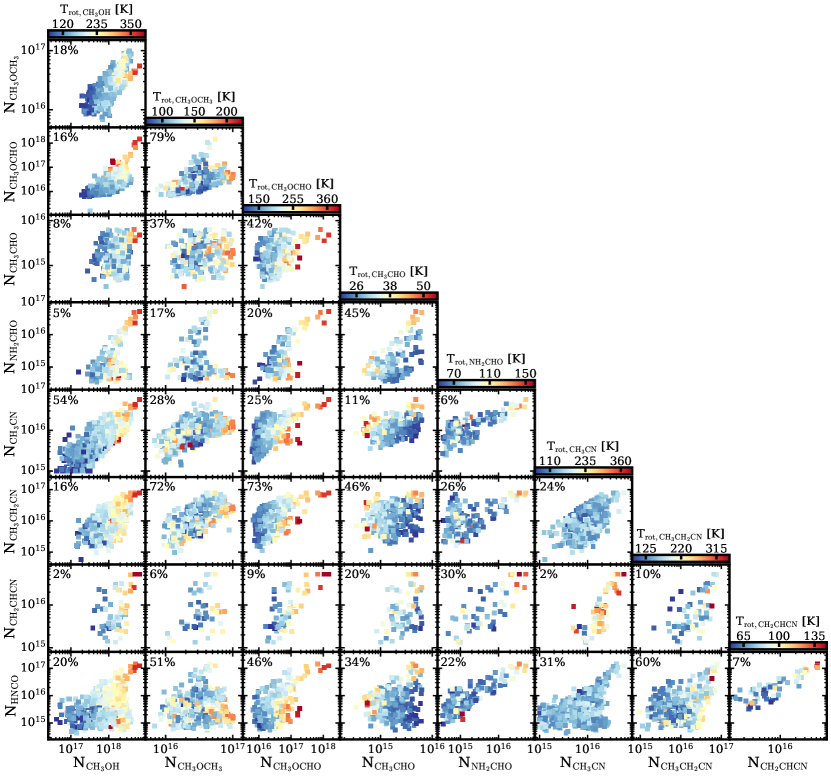
Figure 12: Column densities of each molecule plotted against one another. The color-coding corresponds to the derived rotational temperature of the species on the x-axis, as indicated by the colorscale at the top of each column. The secondary temperature component of CH₃CH₂CN is shown. Percent overlap, as defined in the text, is shown in the upper left corner of each panel.

The majority of species have positive trends, but are not well-described by a single relation and instead exhibit complex trends with multiple components. One notable exception to this trend is CH₃CHO, which is largely uncorrelated with all other species. To leverage the additional information provided by rotational temperatures, we also color-coded the scatter points by temperature. Two distinct hot temperature components are frequently observed: one which can be attributed to HC1, where the highest column densities and hot temperatures are typically observed, and a second from B5, which hosts the strongest H30$\alpha$ line emission, where we often see the hottest temperatures but more moderate column densities. The CH₃CHO/CH₃CN correlation plot is a good example of this phenomenon; the highest rotational temperatures are found in the upper right corner, signifying peak column densities for both species in HC1, and in a grouping of points corresponding to intermediate column densities, attributable to B5. Additional examples of these two hot temperature components are seen in the majority of CH₃OCHO correlations (e.g., CH₃OCHO/CH₃CN, CH₃OCHO/CH₃CH₂CN) and in a few correlations involving CH₃OH (e.g., CH₃OCH₃/CH₃OH).

While strong correlations are observed for numerous species, such as NH₂CHO and CH₂CHCN, we caution broad interpretation of these trends. As reflected in the small percentage (${\lesssim}10$%) of mutual pixels, these trends are only applicable toward the densest regions of gas, namely HC1 and HC2. A good example of this is the correlation between CH₂CHCN/HNCO, which is the highest correlation observed (0.95), but only has a 7% pixel overlap. This indicates that such a correlation is applicable to a minimally-shared region between HNCO and CH₂CHCN, which in this case is HC1, HC2, and a few small patches of gas toward B3. However, some strongly-correlated molecules show a single component with high percentage overlap, such as CH₃OH and CH₃CN, which indicates co-formation across a wide range of environments.

4.4 Rotational Temperature versus Column Density

Next, we investigated the relationship between rotational temperature and column density in each species in Figure 13. Temperature and density trends within a single species not only help characterize the gas excitation conditions present in G10.6, but can also reveal the presence of additional chemical formation and destruction pathways.

Although most species display a positive relation between T_rot and N_col, there is a large range in the relative strength of this association. In general, a large fraction of the gas in N-bearing species, such as CH₃CN, is relatively insensitive to rotational temperature, while the column densities of O-bearing species, such as CH₃OH and CH₃OCHO, are highly correlated with gas temperature. However, this trend is less clear for CH₃OCH₃ and further illustrates its distinct temperature and column density distributions. CH₃CHO and, to a lesser degree, NH₂CHO display negative associations with temperature and are notable outliers to this overall positive T_rot–N_col trend.

To assess spatially-dependent trends, regions of interest were color-coded in Figure 13. HC1 exhibits a distinct and tightly positive correlation between temperature and column density for all species, except for CH₃CHO and CH₃OCH₃. The diffuse correlation seen in CH₃CHO is due to its noisier column density map and likely does not reflect true gas conditions. For CH₃OCH₃, HC1 still exhibits a relatively tight T_rot–N_col association but the largest column densities are instead found in the molecular ridge. The existence of two well-defined HNCO trends in HC1 arises from the complex, dual-peaked temperature structure seen in Figure 8.

HC2 and B3 span a range of different T_rot–N_col associations, from extremely diffuse correlations (CH₃CN, HNCO) to tight positive relations (CH₃OH, CH₃OCHO) and even negative trends (CH₃CHO, NH₂CHO). No clear trends were identified among different types of molecules for either region. Although not labeled in Figure 13, a diffuse component of high rotational temperature but modest column density gas is seen in several species, such as CH₃OH, CH₃OCH₃, CH₃CN, and HNCO, and corresponds to B5.

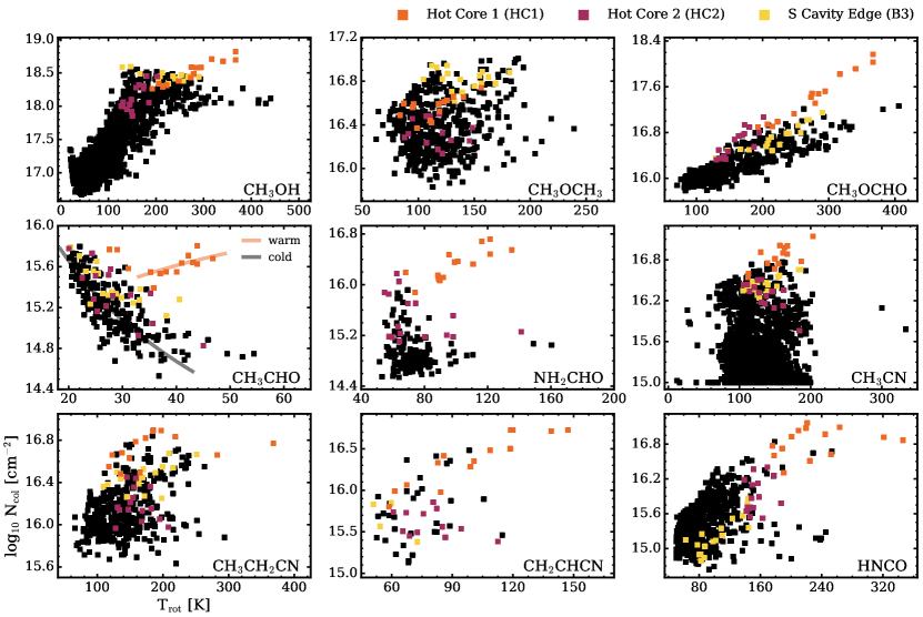
Figure 13: Rotational temperature versus column density for each molecule in our sample. Regions of interest are colored according to the legend. The secondary temperature component is shown for CH₃CH₂CN. Trend lines for CH₃CHO illustrate the presence of a two-component temperature correlation. We note that the CH₃OH data closely resemble the temperature-abundance trend reported in Ginsburg et al. (2017) in massive star-forming region W51 e2.

5 Discussion

5.1 Spatial Distribution of N- versus O-bearing Species

Spatial separations between N- and O-bearing COMs have been observed toward several high-mass star-forming regions, such as Orion (Blake et al., 1987; Wright et al., 1996; Beuther et al., 2005; Feng et al., 2015), W3(OH)/W3(H₂O) (Wyrowski et al., 1999), G19.61-0.23 (Qin et al., 2010), and AFGL 2591 (Jiménez-Serra et al., 2012). However, efforts to assess the ubiquity of such separations with single-dish surveys have so far proved inconclusive (Fontani et al., 2007; Suzuki et al., 2018), but rather require interferometric observations, which can resolve small-scale chemical variations to identify and explain such spatial trends (e.g., Tercero et al., 2018; El-Abd et al., 2019). Here, we aim to test whether chemical differentiation is seen on small scales throughout G10.6 and investigate observed COM spatial trends.

Although we find no evidence for systematic small-scale separations between N- and O-bearing COMs in G10.6, we identify several correlations within and between these molecular families. The observed spatial correlations among the O-bearing species CH₃OH, CH₃OCH₃, and CH₃OCHO probably reflect intrinsic chemical similarity, related formation pathways (see Table 5.2.1), and have been previously seen in several MYSOs (e.g., Bisschop et al., 2007; Brouillet et al., 2013). We also find a strong spatial correlation between the nitriles CH₃CN and CH₃CH₂CN. Together with their high column densities, this likely implies a formation route via grain surfaces (e.g., Mookerjea et al., 2007). Previous models have suggested grain surface hydrogenation and evaporation of accreted CH₃CN and HC₃N to form CH₃CH₂CN (Charnley et al., 1992; Caselli et al., 1993), but based on studies reporting nitrile predictions, these pathways under-produced CH₃CN and CH₃CH₂CN abundances (Caselli et al., 1993; Millar et al., 1997). These small-scale observations strongly suggest that, however complex nitriles form, the formation pathways of medium and large nitriles are linked.

CH₃OH and CH₃CN, the most spatially extended O- and N-bearing species, respectively, in our sample, possess similar spatial distributions and tight column density correlations across G10.6. This is surprising as prior observations of MYSO have reported a lack of correlation between these species (Bisschop et al., 2007; Öberg et al., 2014), and both molecules are thought to form via different mechanisms (Garrod & Herbst, 2006; Garrod et al., 2008). Indeed, in G10.6, we believe the observed correlation likely reflects that both species are tied to total gas column density, rather than intrinsic chemical similarity.

5.2 Relationships between Specific Molecules

During our analysis, we noticed three trends that are further explored here: the complex relationship between CH₃OCHO and CH₃OCH₃, tight correlation between HNCO and NH₂CHO, and unique temperature dependence of CH₃CHO.

5.2.1 CH₃OCHO and CH₃OCH₃

Previous observations of CH₃OCHO and CH₃OCH₃ have revealed nearly constant abundance ratios across a wide range of sources (Jaber et al., 2014; Rivilla et al., 2017; Coletta et al., 2020), remarkably similar spatial distributions (Brouillet et al., 2013), and comparable column densities and gas temperatures (Rong et al., 2016; El-Abd et al., 2019). A chemical link had been previously predicted by modeling (Garrod & Herbst, 2006; Garrod et al., 2008) and experimental efforts (Öberg et al., 2009), which indicated a common precursor hypothesis for the formation of CH₃OCH₃ and CH₃OCHO as either involving the CH₃O radical (solid phase/ice) or CH₃OH${}_{2}^{+}$ (gas phase). Both species can also form through gas-phase chemistry at low temperatures (Balucani et al., 2015), while the presence of additional warm gas-phase pathways cannot be excluded. A summary of the most commonly considered formation routes is provided in Table 5.2.1.

Since all proposed formation pathways each involve the presence of CH₃OH and its photodissociation products, it is unsurprising that we observe strong correlations between CH₃OH and both CH₃OCH₃ and CH₃OCHO, respectively, as shown in the bottom panels of Figure 14. For instance, we identify a nearly constant ratio of CH₃OCH₃ with respect to CH₃OH of 2%, which indicates co-formation or a constant conversion of CH₃OH into CH₃OCH₃ at all temperatures. Constant CH₃OCH₃/CH₃OH ratios have been previously observed in MYSOs (Öberg et al., 2014) and suggest the existence of a single link between CH₃OH and CH₃OCH₃. The simplest explanation for this trend is co-desorption of the two ice constituents, following partial conversion of CH₃OH into COMs, including CH₃OCH₃. If so, this ratio serves as an indicator of overall efficiency of conversion of simple ices into more complex ones. Compared to the typical MYSOs ratios of 14% from Öberg et al. (2014), G10.6 appears to be relatively inefficient in its CH₃OCH₃ ice conversion. In contrast to CH₃OCH₃, the CH₃OCHO/CH₃OH ratio exhibits a multi-component trend that is not well-described by a constant value and cannot be explained by ice chemistry alone. This suggests the presence of multiple formation pathways, and perhaps a mixture of ice and gas-phase chemistry.

The top panels of Figure 14 show the column density correlation between CH₃OCHO/CH₃OCH₃. We identify a broad one-to-one correlation across G10.6, and then a second, much steeper correlation in both HC1 and HC2, where CH₃OCHO is over-produced compared to CH₃OCH₃. This one-to-one correlation agrees remarkably well with the power law relation derived by Jaber et al. (2014) across a wide set of ISM sources over many orders of magnitude in column density and is consistent with observed ratios toward hot cores, intermediate-mass star-forming regions, and hot corinos associated with low-mass protostars (Rivilla et al., 2017, and references therein). As this correlation is quite broad over a wide range of CH₃OCHO temperatures (60–275 K) and physical locations across G10.6, it is difficult to discern the relative importance of various reactions, e.g., cold versus warm gas versus ice surface chemistry, which in principle, may all contribute at some level to this trend without performing detailed chemical modeling. Regardless of their specific formation mechanisms, CH₃OCHO and CH₃OCH₃ seem to behave in the same way within the bulk of gas, i.e., outside of the hot cores, in G10.6 as they do in many other ISM sources.

The presence of an additional component in the CH₃OCHO/CH₃OCH₃ correlation indicates that this chemical similarity does not extend in the same way to the hot cores in G10.6. While this component is most distinctly associated with HC1, it may also extend to HC2, as shown in the top left panel of Figure 14. Moreover, it is not clear if this trend is being driven by gas temperature or is specific to hot core-like environments. We find that the majority, but not the entirety, of points within this steep trend exhibit temperatures ${>}$275 K. To explain the presence of this trend, we must disentangle the relative contribution of increased CH₃OCHO production versus more efficient CH₃OCH₃ destruction. Interestingly, we do find a steepening of the CH₃OCHO/CH₃OH correlation and a modest shallowing of the CH₃OCH₃/CH₃OH correlation towards higher CH₃OH column densities. This suggests that there is an additional CH₃OCHO formation pathway that kicks in within the hot cores, which would also explain the bimodal correlation between CH₃OCH₃ and CH₃OCHO. Further support for the idea that increased CH₃OCH₃ destruction is not driving the observed high CH₃OCHO/CH₃OCH₃ ratio is found in the models of Garrod et al. (2008), which predict a peak gas-phase abundance of CH₃OCH₃ at ${\sim}$200 K. Combined with the fact that CH₃OCH₃ exhibits its highest column densities in the MR, which is exposed to strong radiation fields from the nearby ionized gas in B5, it is unlikely that CH₃OCH₃ is being readily destroyed from high temperatures within the hot cores.

Observations of anti-correlations between CH₃OCHO and formic acid in Orion-KL (Neill et al., 2011a; Brouillet et al., 2013) have suggested that the production of CH₃OCHO is driven by gas-phase reactions (pathway 3 in Table 5.2.1) at high gas temperatures. In support of this explanation, ice chemistry pathways are not thought to be efficient at high temperatures, as the models of Garrod et al. (2008) predict a peak CH₃OCHO abundance at relatively low temperatures (${\sim}$80 K). Thus, one possible explanation for this additional, hot core-dominated trend in G10.6 is gas-phase reactions driving extra production of CH₃OCHO. If CH₃OCH₃ is forming via ice conversion, which is supported by the constant, temperature-independent CH₃OCH₃/CH₃OH ratio across G10.6, i.e. inside and outside hot cores, then provided that the CH₃OCHO gas-phase reaction is sufficiently efficient, this would naturally explain the existence of the observed steeper trend.

Table 4: Chemical Pathways of Interest

[-.3cm]    COM	Num.	Pathway	Type	Ref.
CH3OCHO	[1]	O $+$ CH3OCH2 $\to$ CH3OCHO $+$ H	Cold Gas	1
	[2]	CH3O $+$ HCO $\to$ CH3OCHO	Ice Surface	2, 3
	[3]	CH3OH${}^{+}_{2}$ $+$ HCOOH $\to$ CH3OCHO	Warm Gas	4
CH3OCH3	[4]	CH3O $+$ CH3 $\to$ CH3OCH3 $+$ photon	Cold Gas	1
	[5]	CH3O $+$ CH3 $\to$ CH3OCH3	Ice Surface	5
	[6]	CH3OH${}^{+}_{2}$ + CH3OH $\to$ CH3OCH3	Warm Gas	6
NH2CHO	[7]	HNCO $+$ H $+$ H $\to$ NH2CHO	Ice Surface	7
	[8]	NH2 + HCO $\to$ NH2CHO	Ice Surface	8, 9
	[9]	NH3 + CO $\to$ NH2CHO	Ice Surface	8, 10
	[10]	H2CO $+$ NH2 $\to$ NH2CHO $+$ H	Warm Gas	11, 12
CH3CHO	[11]	CH3 $+$ HCO $\to$ CH3CHO	Ice Surface	13
	[12]	CH3CH2 $+$ O $\to$ CH3CHO $+$ H	Warm Gas	14

Note. — References: (1) Balucani et al. (2015); (2) Garrod et al. (2008); 3) Laas et al. (2011); (4) Neill et al. (2011b); (5) Öberg et al. (2010); (6) Charnley et al. (1995a); (7) Charnley (1997); (8) Jones et al. (2011); (9) Fedoseev et al. (2016); 10 Rimola et al. (2018); (11) Kahane et al. (2013); (12) Barone et al. (2015); (13) Garrod & Herbst (2006); (14) Charnley (2004)

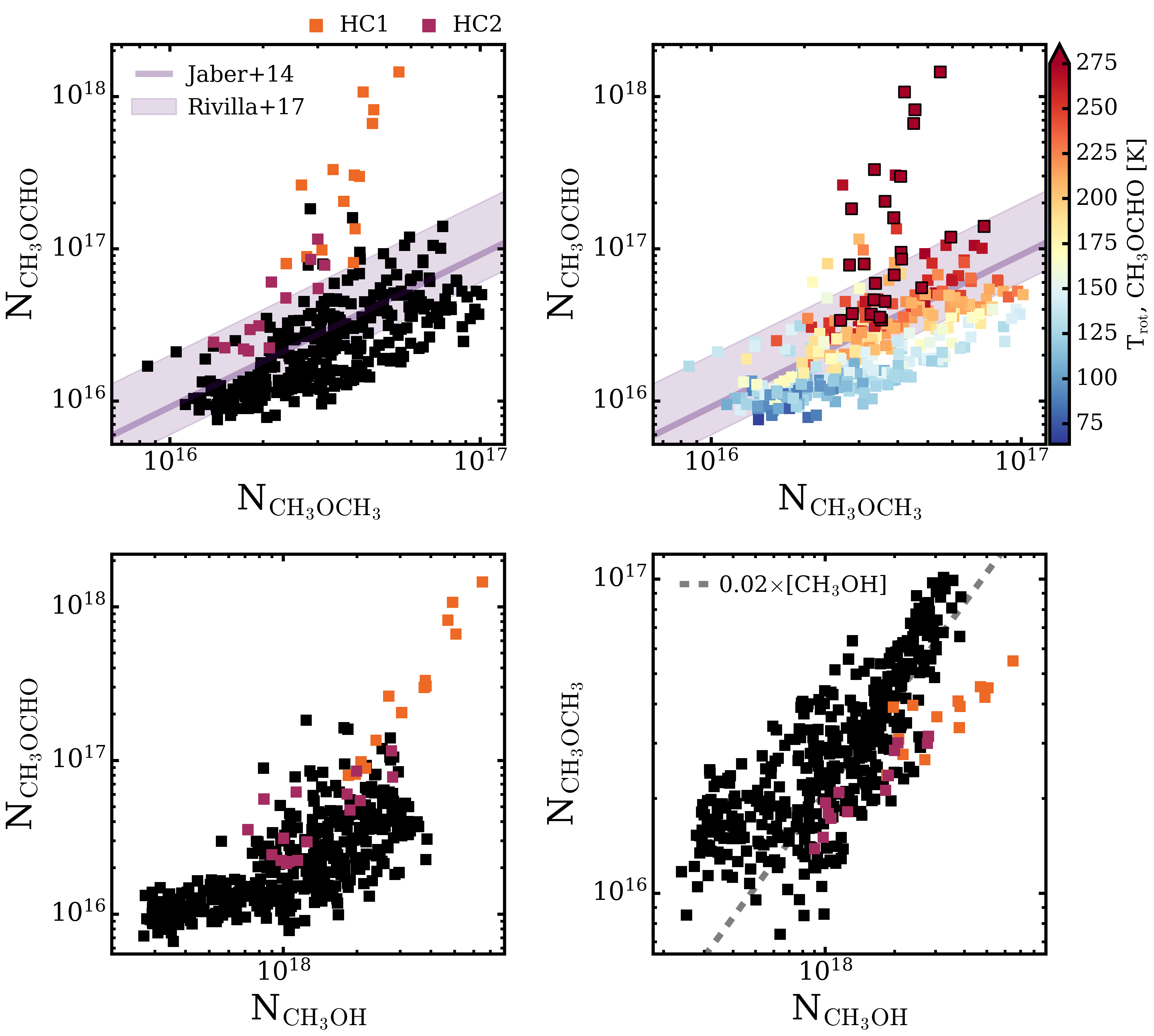
Figure 14: Column density correlations between CH₃OCHO and CH₃OCH₃ (top panels), and with respect to CH₃OH (bottom panels). Power law relation from Jaber et al. (2014) is shown as a solid purple line, while observed ratios from Rivilla et al. (2017) are shaded. HC1 and HC2 are colored in orange and purple, respectively, while all other gas is shown in black. Color-coding is with respect to CH₃OCHO rotational temperature and all points with $\rm{T}>275$ K are shown in dark red and outlined with black borders. Dashed gray line indicates a constant ratio of CH₃OCH₃/CH₃OH of 2%.

5.2.2 HNCO and NH₂CHO

Single dish observations, which found a constant abundance HNCO/NH₂CHO ratio in a range of source luminosities and masses (Bisschop et al., 2007; López-Sepulcre et al., 2015), suggested that these molecules were chemically-related. Evidence of co-spatial emission in the low-mass protobinary system IRAS 16293 (Coutens et al., 2016), two high-mass cores in G35.20 (Allen et al., 2017), and six cores across three massive star-forming regions (Allen et al., 2020) further indicated a link between the two species.

Figure 15 illustrates the observed HNCO/NH₂CHO column density correlation across G10.6. This correlation is strong with a Pearson’s correlation coefficient of $r=0.87$ and extends more than two orders of magnitude in NH₂CHO and three orders of magnitude in HNCO. It is well-characterized by a single power law given by [N${}_{\rm{NH}{{}_{2}}\rm{CHO}}]=0.01\times[\rm{N}_{\rm{HNCO}}]^{1.09}$. Neither HC1 nor HC2 exhibits any significant deviations from this trend, which also appears insensitive to temperature with HNCO rotational temperatures spanning approximately 200 K. In addition, NH₂CHO/HNCO ratios within G10.6 closely resemble those previously observed in a sample of low- and intermediate-mass prestellar and protostellar objects (López-Sepulcre et al., 2015). This consistency is further illustrated in the spatially-resolved NH₂CHO/HNCO ratio map shown in Figure 16. The majority (60%) of our map is consistent with the ratios derived in López-Sepulcre et al. (2015) The highest NH₂CHO/HNCO ratios, which show the largest deviations, are mostly located at peripheries, where NH₂CHO line intensities are weaker and uncertainties correspondingly elevated.

The spatial distributions of both species also provides valuable information about their formation mechanisms. As noted in Section 4.2, column density maps show that HNCO is more spatially extended relative to NH₂CHO. Specifically, NH₂CHO is never observed in a region lacking HNCO emission. Not only does NH₂CHO possess a spatially-limited column density map, it also displays the most compact integrated intensity map of all COMs in our sample (Figure 2). Particularly salient is the absence of any detectable NH₂CHO toward B3, which otherwise exhibits emission from all other COMs, including HNCO, in our sample. Although difficult to disentangle from the intrinsic excitation characteristics of each species, i.e., Table 3.1, this nonetheless seems to suggest that the formation of NH₂CHO in detectable amounts depends on the presence of hot core-like physical environments and not simply on the presence of HNCO.

A variety of explanations have been put forth to explain the empirical relationship between HNCO and NH₂CHO. Charnley (1997) suggested that NH₂CHO forms via the hydrogenation of HNCO, but this route has been challenged by subsequent experimental work (Noble et al., 2015). Simultaneously formation in ices has been explored experimentally (Jones et al., 2011; Fedoseev et al., 2016; Ligterink et al., 2018), and gas-phase pathways (Kahane et al., 2013; Barone et al., 2015; Codella et al., 2017) have also been proposed. Other models (Quénard et al., 2018) argue that the observed HNCO/NH₂CHO correlation is instead due to both species responding in similar ways to physical parameters, such as temperature, rather than a direct chemical link between the two species. In light of this finding, the strong correlation observed here warrants a further investigation into the relationship between these molecules in G10.6.

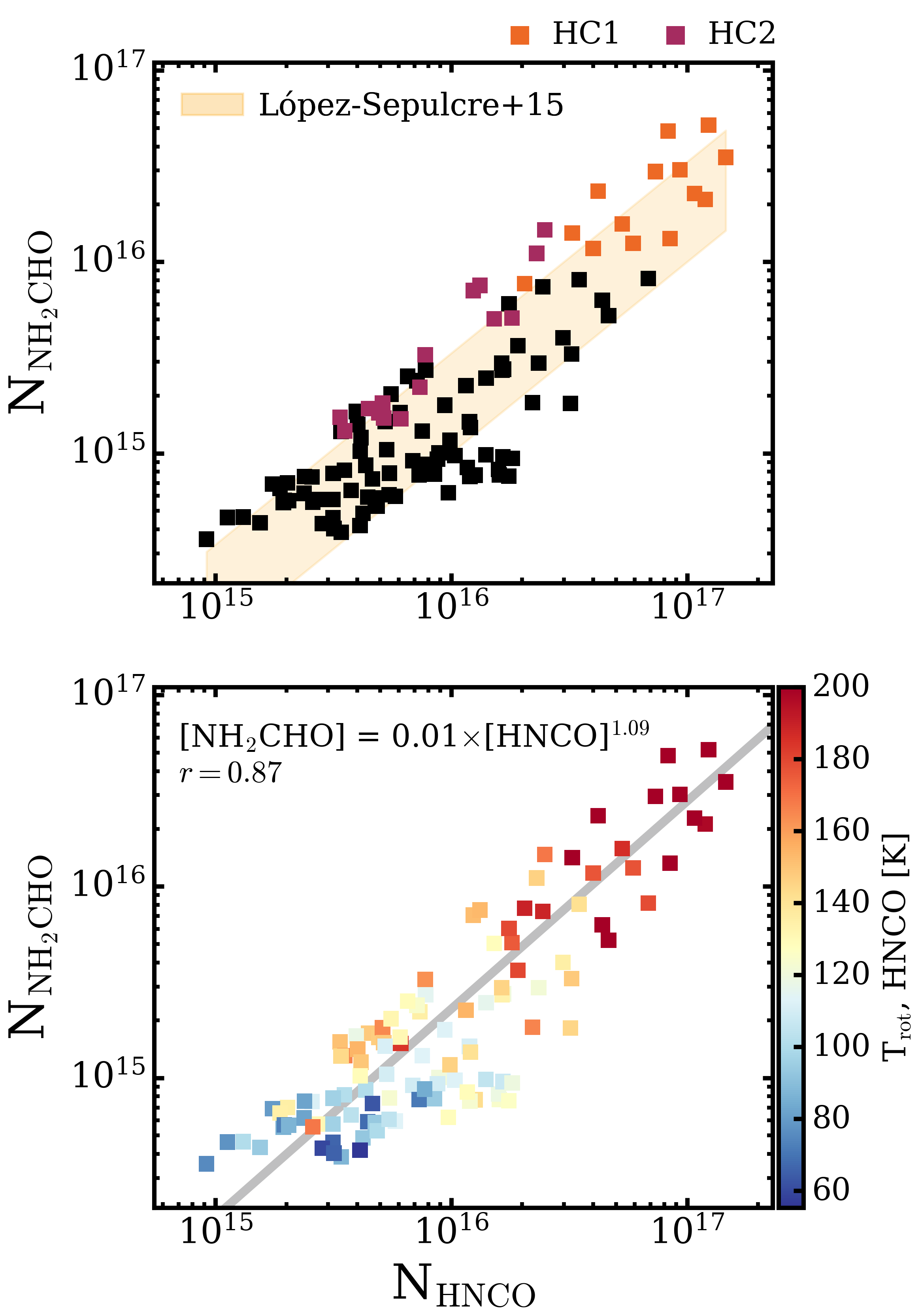
Figure 15: HNCO/NH₂CHO column density ratios in G10.6. Top: Observed column density ratios closely resemble those reported in López-Sepulcre et al. (2015) for a sample of low- to intermediate-mass prestellar and protostellar objects. HC1 and HC2 are colored in orange and purple, respectively. Bottom: Column densities ratios color-coded according to HNCO rotational temperatures. Best fit power law and correlation coefficient are shown.

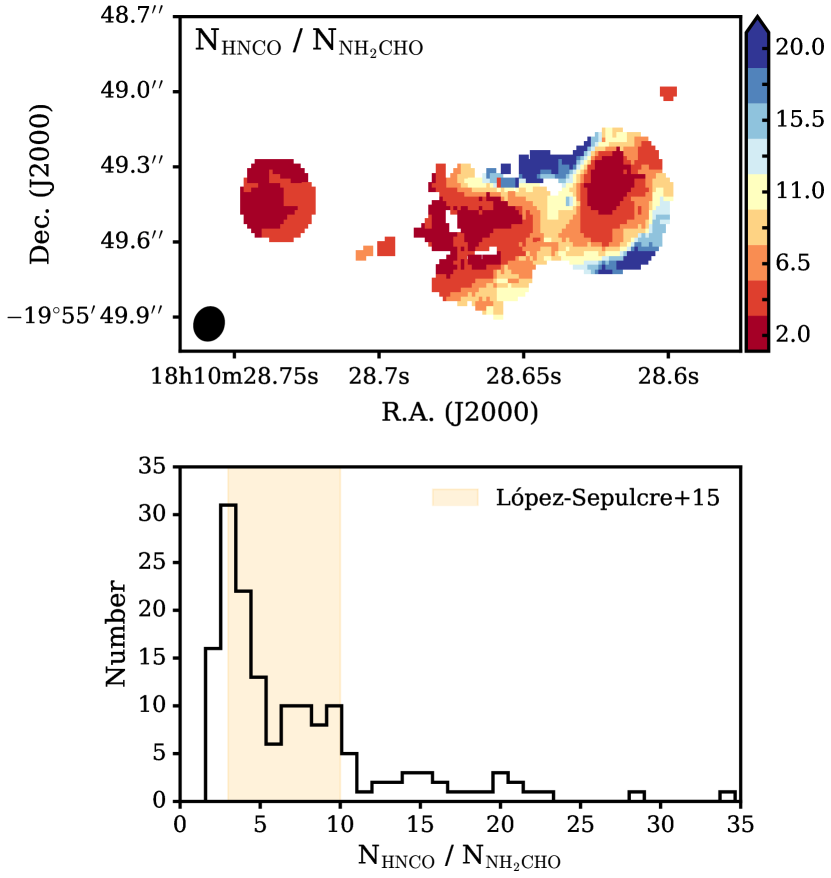
Figure 16: HNCO/NH₂CHO column density ratios for regions of mutual overlap in G10.6 (top) and histogram of derived ratios (bottom), relative to those reported in López-Sepulcre et al. (2015).

5.2.3 CH₃CHO

Based on both single-dish and spatially-resolved observations of MYSOs, Öberg et al. (2014) found that CH₃CHO displays an overall negative dependence on temperature. Specifically, at low column densities and temperatures (${<}$100 K) the CH₃CHO/CH₃OH ratio was almost constant at a few percent, which then dropped dramatically by several orders of magnitude when ${>}$100 K. However, several outliers in the form of high CH₃CHO/CH₃OH ratios even at ${>}$100 K hinted at the presence of an additional high temperature formation pathway for CH₃CHO. Notably, all of these outliers were derived from spatially-resolved observations, which suggests that these increased CH₃CHO abundances may be a common feature of hot core chemistry.

We observe the presence of two such CH₃CHO formation pathways explicitly in G10.6, as shown in Figure 13, where superimposed trend lines are shown to illustrate the presence of these two distinct components. A positive association with temperature is only found in HC1, which indicates the activation of a lukewarm formation pathway at approximately 30 K. Outside of HC1, we see a tight negative correlation with temperature, indicating that the bulk of the CH₃CHO gas is forming via this cold route, and perhaps rapidly degrades in lukewarm regions. Thus, single-dish studies, or otherwise low-spatial resolution observations of MYSOs that cannot resolve hot cores, would likely be dominated by this cold component.

Although less pronounced than in CH₃CHO, there is evidence of a similar two component formation pathway for NH₂CHO. The bulk of NH₂CHO in G10.6 seems to form efficiently at low temperatures (50–90 K), while in HC1, an extremely tight, positive association with temperature is present. This hot core component becomes activated around 60 K and continues until nearly 150 K. Thus, there likely exists an efficient low-temperature formation pathway for these molecules, which decreases in efficiency with temperature, but then at very elevated temperatures, the species are released from the ice, along with the majority of COMs, resulting in high abundances in HC1.

The formation route of CH₃CHO remains unclear, as the relative contribution of gas-phase and grain surface chemistry is not well understood. Grain surface models (Garrod & Herbst, 2006; Garrod, 2013) and laboratory experiments (e.g., Bennett et al., 2005; Öberg et al., 2009) have predicted that CH₃CHO forms via the combination of radicals CH₃ and HCO on grain mantles. However, recent quantum chemistry computations by Enrique-Romero et al. (2016, 2019) show that this may be inefficient, as additional pathways resulting in CH₄ and CO are competitive. Alternatively, gas-phase models suggest oxidation of hydrocarbons as the primary formation route. Specifically, the release of C₂H₆ from dust surfaces is expected to drive production of CH₃CH₂, which in turns reacts in the gas phase with atomic oxygen to form CH₃CHO (Charnley, 2004). A summary of these proposed ice surface and gas-phase formation pathways is listed in Table 5.2.1.

De Simone et al. (2020) showed that a gas-phase route is responsible for CH₃CHO production in the outflows of NGC 1333 IRAS 4A. The rotational temperatures (${\sim}$10–30 K) in these outflows are comparable to those associated with the low temperature component in G10.6, which suggests that the bulk of CH₃CHO gas may also be forming via gas-phase reactions. A similar finding was reported by Codella et al. (2017), in which gas-phase formation of NH₂CHO was confirmed in L1157-B1. Since the temperatures (20–80 K) associated with the B1 cavities (e.g., Gómez-Ruiz et al., 2015) are similar to those in the cold component of NH₂CHO, this again may point to gas-phase formation. Although extrapolating conclusions from regions of shock chemistry is not without caveats, these results nonetheless suggest that both cold components for CH₃CHO and NH₂CHO have their origins in gas-phase reactions in G10.6.

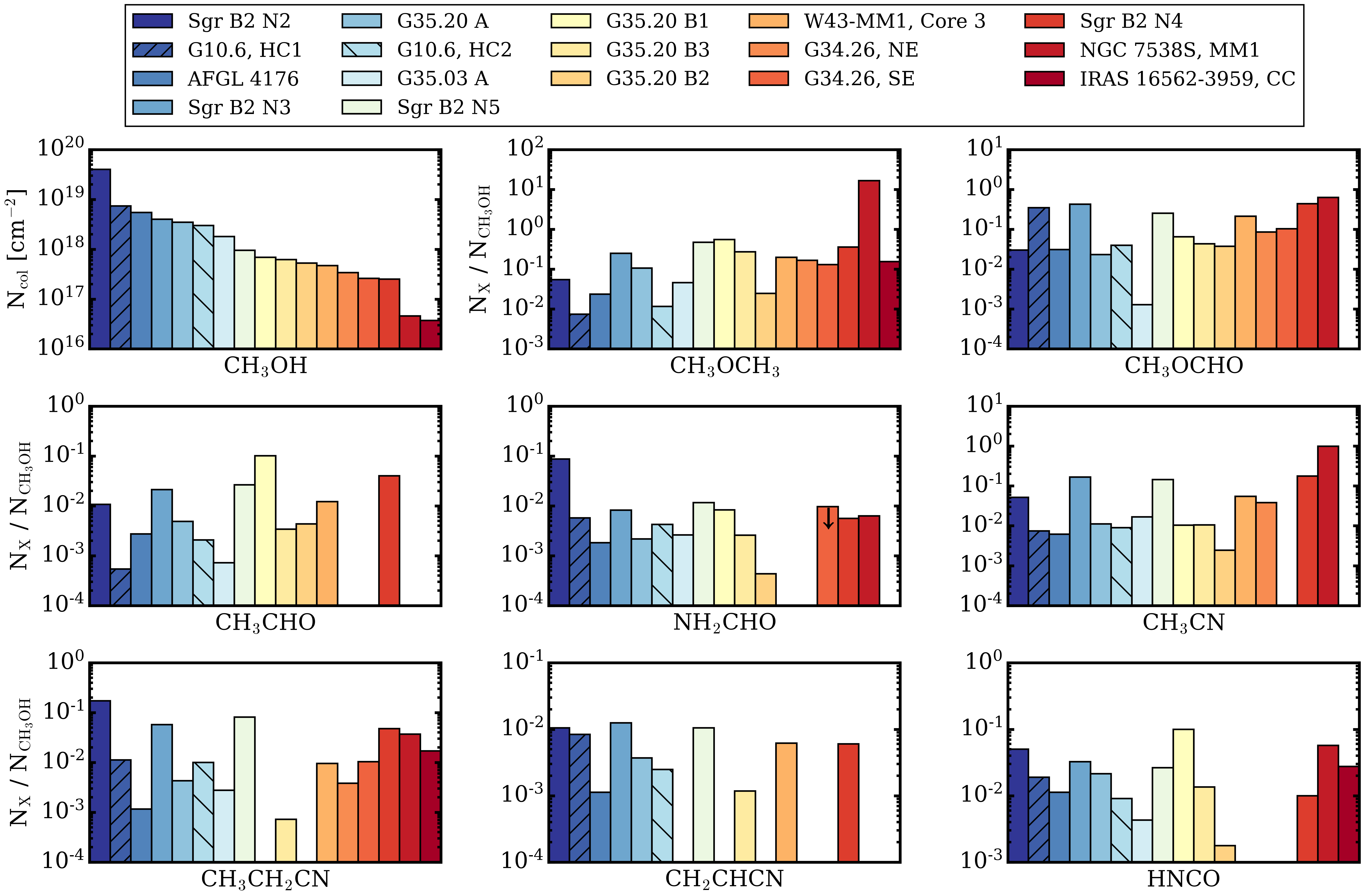
Figure 17: Comparison of column densities with respect to CH₃OH of HC1 and HC2 in G10.6 versus a large sample of spatially-resolved MYSOs observations compiled from the literature. Sources are ordered by descending CH₃OH column density and upper limits are indicated by downward arrows. When the column density of a species is not reported in the literature, no bar is shown and no attempt was made to derive upper limits when not provided.

5.3 Comparisons with Other Sources

5.3.1 Massive Star-forming Regions

To quantify how typical HC1 and HC2 in G10.6 are relative to other well-known MYSOs, we compared them against spatially-resolved data from: AFGL 4176 (Bøgelund et al., 2019); G34.26 (Mookerjea et al., 2007); G35.20 A, B1–3 and G35.03 A (Allen et al., 2017); IRAS 16562-3959, central compact (CC) core (Guzmán et al., 2018); NGC 7538S, MM1 (Feng et al., 2016); Sgr B2, N2–5 (Bonfand et al., 2017, 2019); and Core 3, W43-MM1 (Molet et al., 2019).

Figure 17 shows the fractional abundances with respect to CH₃OH of G10.6 and the literature sample. Both G10.6 cores have relatively high CH₃OH column densities (${>}10^{18}$ cm^-2), which place them in the top half of the comparison sample. Both cores also exhibit the two lowest CH₃OCH₃ abundances, while HC1 possesses the lowest CH₃CHO abundance and HC2 is 4th lowest. However, besides these two species, both HC1 and HC2 are consistent with literature values and both appear quite typical for massive cores in their relative compositions.

We next explore COM column density ratios, which often serve as important signposts of evolutionary state and provide constraints on the chemistry occurring within particular sources (e.g., Fontani et al., 2007; Suzuki et al., 2018). Figure 18 compares column density ratios in both hot cores with those in the literature sample of MYSOs. HC1 and HC2 consistently deviate by up to two orders of magnitude from the MYSO sample in ratios among CH₃CHO, CH₃OCH₃, and CH₃OCHO. These discrepancies are readily understood by recalling that in Figure 17, HC1 and HC2 are shown to be unusually poor in CH₃CHO and CH₃OCH₃, and present CH₃OCHO abundances in the upper range of what has been previously observed. In addition, HC1 may be unusual in its efficient CH₃OCHO formation, perhaps due to unique conditions favoring gas-phase formation (see Section 5.2.1).

The range of ratios exhibited by N-bearing species, such as CH₂CHCN/HNCO, NH₂CHO/HNCO, and NH₂CHO/CH₂CHCN, is substantially narrower than that of O-bearing COMs. In particular, HC1 and HC2 appear more typical relative to other MYSOs, and more consistent with each other, i.e. within factors of a few, in their overall N chemistry. The one exception to this trend is that of the complex cyanides, namely the CH₃CN/CH₃CH₂CN and CH₃CN/CH₂CHCN ratios, which are elevated in both HC1 and HC2.

The ratio between CH₂CHCN and CH₃CH₂CN is sensitive to physical parameters of hot cores (Caselli et al., 1993) and has been used as an estimator of evolutionary age (e.g., Fontani et al., 2007). We find CH₂CHCN/CH₃CH₂CN ratios of 0.49$\pm$0.30 and 0.23$\pm$0.04 for HC1 and HC2, respectively. These are both consistent with the MYSO comparison sample (0.3–0.9), and the values (0.3–0.5) reported in Fontani et al. (2007) for a single-dish survey of well-known hot cores. Since chemical models predict a sharp decrease in the abundances of CH₂CHCN and CH₃CH₂CN after ${\sim}10^{5}$ yr (Caselli et al., 1993), their mutual detection and consistent ratios in both cores suggest that they are younger than ${\lesssim}10^{5}$ yr with HC2 likely being a factor of a few younger than HC1. More specific conclusions require detailed chemical modeling, especially since Charnley et al. (1992) and Rodgers & Charnley (2001) have suggested that additional gas-phase reactions are important for CH₂CHCN production, while Allen et al. (2018) demonstrated that a shorter warm-up phase can also reproduce observed cyanide abundances.

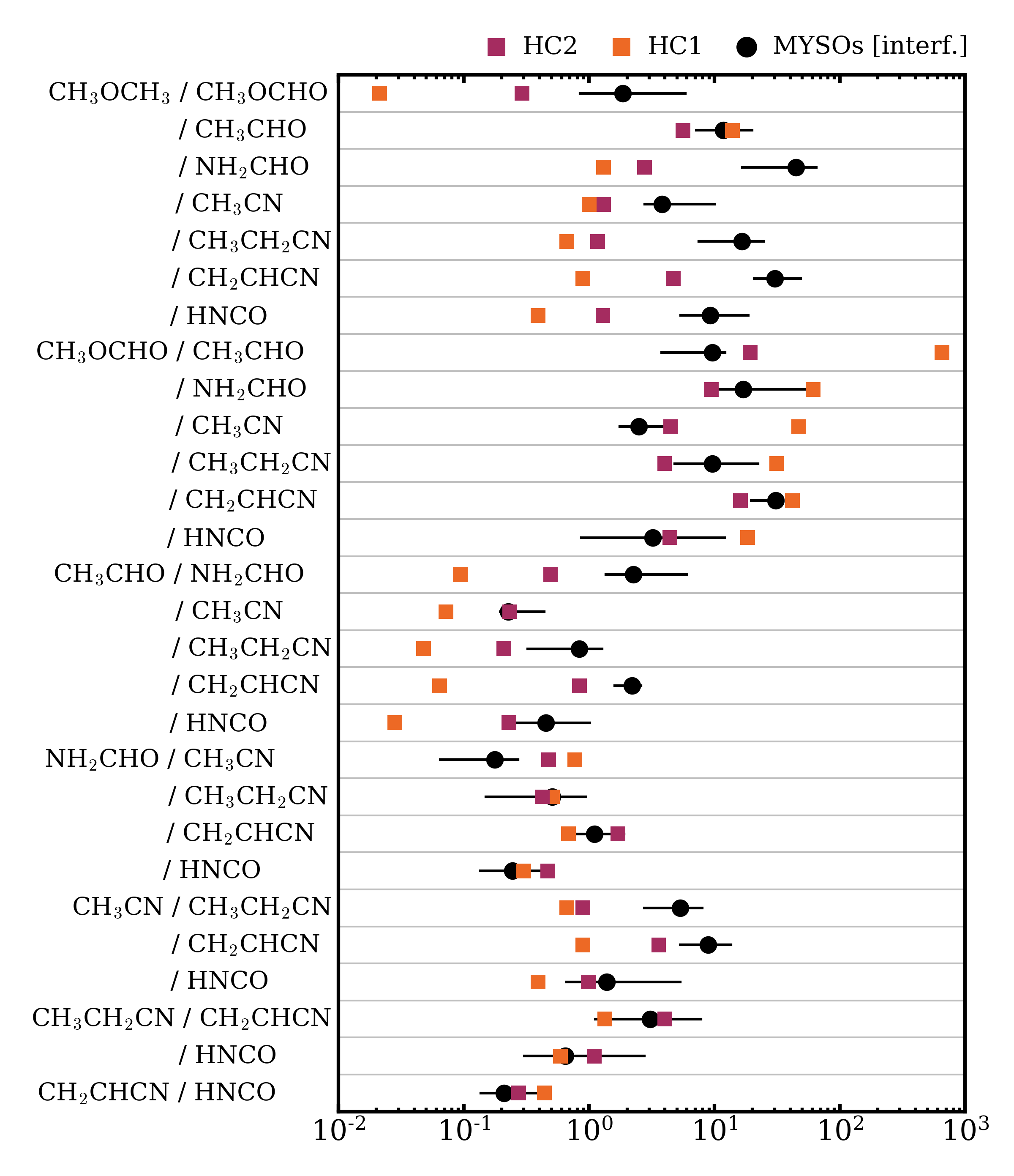
Figure 18: Column density ratios in HC1 and HC2 versus those from the MYSO sample from Figure 17. HC1 and HC2 are shown as orange and purple squares, respectively. Filled black circles denote median MYSO values, while the black lines indicate the upper and lower quartiles.

5.3.2 Galactic Center Clouds, Comets, and Low-mass Star-forming Regions

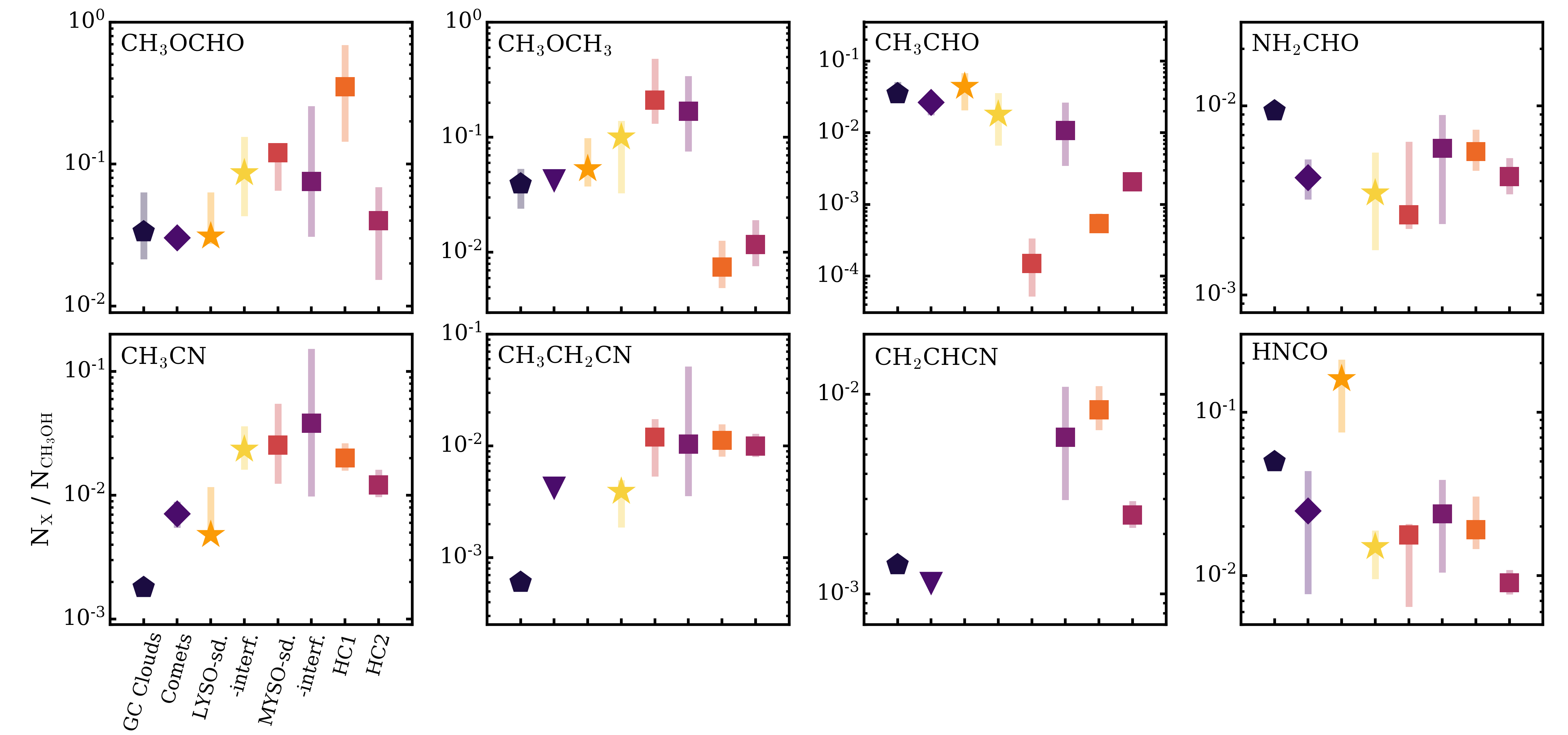
Figure 19: Comparison of COM column densities with respect to CH₃OH. Data are taken from: GC clouds (Requena-Torres et al., 2006, 2008; Zeng et al., 2018); comets (Biver et al., 2014; Biver & Bockelée-Morvan, 2019); LYSOs from single dish (sd.; Bergner et al., 2017) and interferometric (interf.; Belloche et al., 2020) observations; and MYSOs from single dish observations (Taquet et al., 2015, and references therein). The MYSO sample observed with inteferometers is the same as that shown in Figures 17 and 18. The comet data comprise the two well-studied comets C/1995 O1 (Hale-Bopp) and C/2014 Q2 (Lovejoy). Inverted triangles indicate upper limits.

To better understand COM trends across different physical environments, Figure 19 compares COM column densities in HC1 and HC2 with a variety of different ISM sources, including Galactic center (GC) clouds, comets, and low-mass YSOs (LYSOs). COM abundances are remarkably similar across this wide set of sources, which suggests that the underlying chemistry is not greatly sensitive to variations in physical environments. In particular, N-bearing species, e.g., NH₂CHO, CH₃CN, CH₃CH₂CN, exhibit relatively consistent abundances across different types of sources, while O-bearing COMs display larger variations. In particular, CH₃OCH₃ is underabundant by at least an order of magnitude in both hot cores, while CH₃OCHO is enhanced in HC1 by a factor of a few relative to all other sources. These differences are another indicator, similar to the unusual COM ratios seen in Section 5.3.1, of the relative deficits or overabundances in the derived column densities of these species and further establish their relative significance.

CH₃CHO exhibits the largest spread across source types. Öberg et al. (2014) found that spatially-resolved hot cores exhibited higher CH₃CHO/CH₃OH ratios compared to those inferred from single-dish observations. We confirm the existence of this trend by comparing observations of unresolved MYSOs versus those that are spatially resolved. The spatially-resolved values are reduced by up to two orders of magnitude in CH₃CHO/CH₃OH. We do not see a similar trend in the LYSOs, which have nearly the same CH₃CHO/CH₃OH ratios for both types of observations. Based on Figure 19, the majority of other COMs have consistent abundances between their resolved and unresolved samples, which confirms that CH₃CHO/COMs ratios in MYSOs are lower for unresolved observations.

This trend is best understood by first contrasting single dish observations of LYSOs and MYSOs. In the case of LYSOs, large beam sizes result in observations dominated by cold protostellar envelopes, where, due to their low temperatures, CH₃CHO is expected to be abundant. However, this is not the case for MYSOs, which exhibit higher temperatures in their envelopes and surrounding gas structures. But as seen in Öberg et al. (2014) and here in G10.6, there is a rapid fall off in CH₃CHO abundances at warmer temperatures. Moreover, unresolved observations of MYSOs are not sensitive to high CH₃CHO column densities associated with hot core chemistry. The combination of these factors leads to dramatically reduced CH₃CHO/CH₃OH ratios, as is clearly seen in Figure 19. In this scenario, the intermediate CH₃CHO/CH₃OH ratios of HC1 and HC2, i.e., between that of the unresolved and resolved MYSO samples, is naturally explained by the fact that both hot cores are only marginally resolved in our observations of G10.6.

If this explanation is true, we would expect CH₃CHO / CH₃OH ratios in cold clouds, which do not possess hot core chemistry and contain only cold gas, to be comparable or larger to those from single dish studies of LYSOs. Recent observations of several starless and prestellar cores in Taurus by Scibelli & Shirley (2020) provide a helpful comparison sample for this purpose. Scibelli & Shirley (2020) found a median CH₃CHO/CH₃OH ratio of ${\sim}0.09$, which is indeed slightly larger than that associated with single dish studies of LYSOs.

6 Conclusions

We have presented ALMA high spatial resolution observations of the COM chemistry in massive star-forming region G10.6 at 1.3 mm. These observations reveal that while hot core chemistry appears consistent over many different environments, the chemistry of surrounding COM structures is much more varied and complex. Importantly, the discovery of extended COM structures throughout the central 20,000 au region of G10.6 illustrates that COM chemistry is not only confined to hot molecular cores, but is likely more generally associated with massive star-forming regions. The highly-structured nature of these COM features hints at the importance of interactions between hot, ionized gas and nearby surrounding dense gas.

In addition to having important implications for models of such regions (e.g., external heating), our results further reinforce the need for high spatial resolution observations and suggest that the small-scale distributions of COMs can provide crucial insight into the physical and chemical processes associated with massive star formation. These results also highlight the need for more observations at intermediate spatial resolutions, which are sensitive to larger physical scales, to properly characterize COM emission. This is best demonstrated by COMs such as CH₃CHO, for instance, where insufficient resolution, e.g., single dish observations, would not capture core-scale lukewarm chemistry, while very high angular resolutions would instead filter out more extended cold gas chemistry.

We identify a variety of chemical trends, e.g., CH₃OCH₃/CH₃OCHO, HNCO/NH₂CHO, previously observed in samples of diverse ISM sources, to also hold true within G10.6 in a spatially-resolved manner. Moreover, they often behave in the very same way, i.e., power law slopes, column density ratios, as they do in these other sources, suggesting that the underlying COM chemistry is tightly linked. Despite this broad agreement, we also observe several unexpected trends, including a spatial distribution of CH₃OCH₃ that is strikingly dissimilar to that of CH₃OCHO and an overabundance of CH₃OCHO within at least one hot core. These findings suggest that our current understanding of COM chemistry remains incomplete and provide valuable inputs for chemical models.

Appendix A Full Spectral Coverage

Figure 20 shows the remaining half of our spectral coverage toward the same representative positions as in Figure 3.

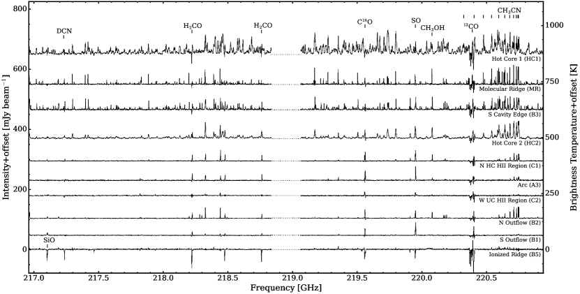
Figure 20: Spectra extracted from single pixels toward the same ten positions in G10.6 as in Figure 3. Dashed line represent gaps in observational coverage between the spectral windows.

Appendix B COM Kinematics in G10.6

In Figure 21, we examine the velocities of the same lines as in Figure 2. We find a coherent velocity gradient of ${\sim}$10 km s^-1 along the NW-SE direction in both individual transitions of single molecules and across the entire sample of species. The velocities of NH₂CHO appear to be systematically blue shifted relative to the other COMs, which may indicate that the emission is originating from a different spatial region due to chemical layering or an expanding or contracting shell of gas. The velocities of CH₃CHO are also modestly blue shifted, and given that both NH₂CHO and CH₃CHO are among the molecules with the coolest temperatures in G10.6, it is possible that they are both arising from a similar region that is distinct from that of the remainder of the warmer COMs.

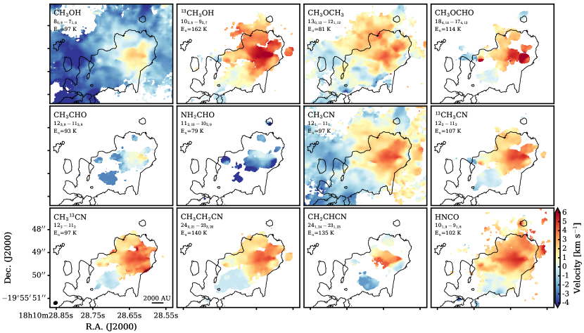
Figure 21: Velocity structure for transitions with E${}_{\rm{u}}\approx 100$ K for all molecules in our sample. The velocity scale in the color bar is the same for all panels. The black contours show the continuum emission at the 10% level.

Appendix C Details of Line Data Analysis

Below, we present a detailed description of the entire analysis process, from the initial pixel-masking to the derivation of rotational temperature and column density maps.

C.1 Line Fitting

Integrated intensities for each observed line were determined by fitting a single Gaussian profile to each feature. For lines with substantial wings, only the central peak was used in deriving column densities. Unresolved multiplets originating from the same species were treated as a single line by combining the degeneracies and line intensities.

For each transition, a mask corresponding to a 5$\sigma$ level in peak intensity in a 10 km s^-1 window centered on the transition frequency was used to define a pixel-by-pixel mask. We obtained initial constraints on line parameters for each species separately based on the most cleanly observed lines. For these initial fits, the FWHM was allowed to vary between 1.3 km s^-1 (i.e., the velocity resolution) and 15 km s^-1, while systemic velocity was restricted to a window centered on the expected transition frequency with a width between $\pm$3–8 km s^-1, depending on the presence of adjacent wings from other transitions or nearby line crowding from other species. For all other lines of a single molecule, the FWHM was restricted to 0.25–1.25$\times$ the FWHM of the template line and the systemic velocity to $\pm$2 velocity channels from the template line position. We note that some variation between lines is expected, even for a single species, due to different excitation conditions of lines with different upper energy levels and Einstein A coefficients.

Since G10.6 is line-rich, blending is occasionally present, especially near regions of denser gas with large linewidths (e.g., HC1, and to a lesser extent, HC2). In general, lines that were not unambiguously free from blending throughout G10.6 are not included in the analysis. For each transition of each species, we randomly selected a set of a few hundred fits across G10.6 and confirmed via visual inspection that the fitting process was accurately capturing the observed line properties. During this process, we removed all blended transitions from the analysis. In a few rare cases, line blending was due to a nearby transition originating from the same species, e.g., the K$=0$ and K$=1$ lines of the J$=$12–11 ladder of CH${}_{3}^{13}$CN. In such cases, we treated them as a single line by fitting a single Gaussian and combining line characteristics.

C.2 Rotational Temperature and Column Density Derivation

For each such pixel, we calculated column density and rotational temperature. Assuming optically thin emission, the column density of molecules in the upper state of each transition $N^{\rm{thin}}_{\rm{u}}$ is related to the emission surface brightness $I_{\nu}$ via:

$$I_{\nu}=\dfrac{A_{ul}N^{\rm{thin}}_{\rm{u}}hc}{4\pi\Delta v},$$ (C1)

where $A_{\rm{ul}}$ is the Einstein coefficient and $\Delta v$ is the linewidth (e.g., Bisschop et al., 2008). Since we are performing this analysis on individual pixels of a certain size, we need to write $I_{\nu}$ in terms of the flux density $S_{\nu}$ and the solid angle subtended by the source $\Omega$ via $I_{\nu}=S_{\nu}/\Omega$ (e.g., Bergner et al., 2018; Loomis et al., 2018). Rearranging Equation C1:

$$N^{\rm{thin}}_{\rm{u}}=\dfrac{4\pi S_{\nu}\Delta v}{A_{ul}\Omega hc}$$ (C2)

where $S_{\nu}\Delta v$ is the integrated flux density for each transition, and we use the pixel size ($0.018^{\prime\prime}$) to estimate the solid angle $\Omega$.

The upper state level population $N_{\rm{u}}$ is related to the total column density $N_{\rm{T}}$ by the equation:

$$\frac{N_{\rm{u}}}{g_{\rm{u}}}=\frac{N_{\rm{T}}}{Q(T_{\rm{rot}})}e^{-E_{\rm{u}}/k_{\rm{B}}T_{\rm{rot}}},$$ (C3)

where $g_{\rm{u}}$ is the degeneracy of the upper state level, $Q$ is the partition function, and $T_{\rm{rot}}$ is the rotational temperature, and E_u is the upper state energy.

The frequencies, line strengths, and upper-state energies of the observed lines of CH₃OH are summarized in Appendix Table E, along with the complete set of unblended lines for all molecules included in our sample. In general, line characteristics were taken from the JPL and CDMS catalogs, as indicated in Table 3.1. We note that catalogs sometime differ in their consideration of nuclear spin in their Einstein A values and partition functions. Care therefore was taken to use matching Einstein A values and partition functions. Partition functions were linearly interpolated from catalog values for all molecules, except for CH₃OCHO, where the relative contributions from the vibrational and torsional states are over 40%. In this case, we used the complete rotational-torsional-vibrational partition function from Carvajal et al. (2019).

As standard in rotational diagram analysis (e.g., Goldsmith & Langer, 1999), taking the logarithm of Equation C3 gives the linear equation:

$$\ln\left(\frac{N_{\rm{u}}}{g_{\rm{u}}}\right)=\ln N_{\rm{T}}-\ln Q(T_{\rm{rot}})-\frac{E_{\rm{u}}}{k_{\rm{B}}T_{\rm{rot}}}.$$ (C4)

A semi-log plot of $N_{\rm{u}}/g_{\rm{u}}$ versus upper state energies E_u allows for the derivation of rotational temperature and total column density from the best fit slope and intercept, respectively. The optical depth of the observed transitions is unknown a priori, and in regions of high density such as G10.6, we may expect optically thick lines. In this case, i.e. $\tau\not\ll 1$, the optical depth correction factor $C_{\tau}$ must be applied:

$$C_{\tau}=\frac{\tau}{1-e^{-\tau}},$$ (C5)

which makes the true level populations:

$$N_{\rm{u}}=N_{\rm{u}}^{\rm{thin}}C_{\tau}.$$ (C6)

With these corrections, Equation C4 can be rewritten as:

$$\ln\left(\frac{N_{\rm{u}}^{\rm{thin}}}{g_{\rm{u}}}\right)+\ln C_{\tau}=\ln N_{\rm{T}}-\ln Q(T_{\rm{rot}})-\frac{E_{\rm{u}}}{k_{\rm{B}}T_{\rm{rot}}}.$$ (C7)

The optical depths of individual transitions can then be related back to the upper state level populations via:

$$\tau_{ul}=\frac{A_{ul}c^{3}}{8\pi\nu^{3}\Delta v}N_{\rm{u}}\left(e^{h\nu/k_{\rm{B}}T_{\rm{rot}}}-1\right).$$ (C8)

Hence, $C_{\tau}$ can be written as a function of $N_{\rm{u}}$ and substituted back into Equation C8 to construct a likelihood function $L(\rm{data},N_{\rm{T}},T_{\rm{rot}})$ to be used for $\chi^{2}$ minimization (e.g., Loomis et al., 2018). Given this likelihood function, we then used the affine invariant MCMC code emcee (Foreman-Mackey et al., 2013) to fit the data and generate posterior probability distributions for N_T and T_rot, which describe the range of possible column densities and rotational temperatures consistent with the observed data. To illustrate this method, Figure 22 shows rotational diagrams for all species in our COM sample toward HC1. Complete rotational diagrams toward HC2, B3, and MR are shown in Figure Set 1, which is available in the electronic edition of the journal.

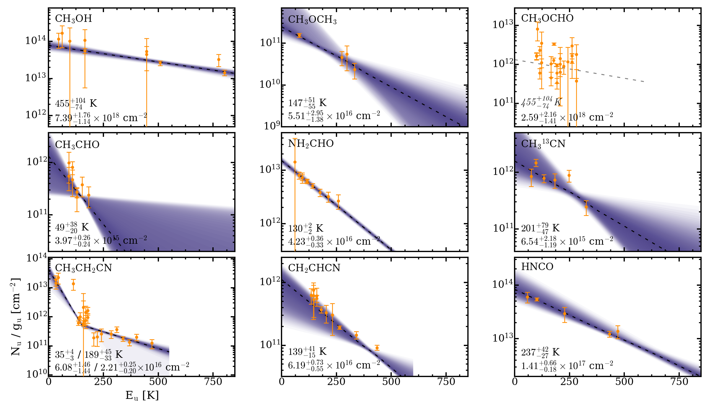
Figure 22: Rotational diagrams for COMs in our sample toward HC1. Transitions are shown in orange and random draws from the fit posteriors are plotted in purple. The fit is indicated by a dashed black line and derived values are shown in the lower left corners. A gray dashed line and italicized rotational temperature indicate that this temperature was adopted from a chemically-similar species, as described in the text. (The complete figure set (4 images) showing rotational diagrams toward four positions of interest in G10.6 is available in the online journal.)

C.3 Line Blending and Example LTE Spectra

To assess the level of blending present, particularly toward dense regions such as HC1, we compared observed spectra with synthetic LTE model spectra generated using the MADCUBA (MAdrid Data CUBe Analysis) package (Martín et al., 2019). We used the SLIM (Spectral Line Identification and LTE Modelling) tool within MADCUBA, which uses spectroscopic data from the CDMS and JPL catalogs to produce model spectra under LTE conditions for a given set of input physical parameters. For each species in our sample, we inputted the rotational temperature, column density, typical FWHM, and systemic velocity, as derived in Section 3. We fixed the source size to the beam size for all molecules and extracted spectra toward HC1 and MR from a region equal in area to the beam size. Figure 23 shows the LTE model spectrum toward HC1, which has the densest gas and largest line widths in G10.6, and thus, we expect maximal line blending to occur toward this region. In general, a moderate degree of line blending is present for some species (e.g., CH₃OCHO), but in all cases, there are a sufficient number of unblended lines to allow for reliable fits and robust rotational diagrams. Next, in Figure 24, we show an LTE spectrum toward the MR, which is more representative of the gas outside of HC1 and HC2 in G10.6. Here, blending is minimal, due in part to the narrower line widths.

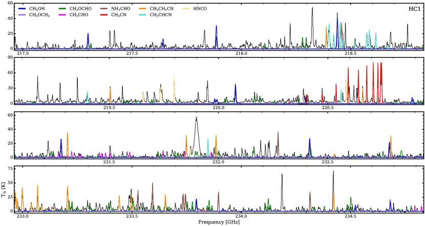
Figure 23: Spectrum toward HC1 extracted from a region equal to the beam size with an overlaid synthetic LTE model spectra from MADCUBA. Different colors represent individual molecules according to the legend.

Figure 24: Spectrum toward MR extracted from a region equal to the beam size with an overlaid synthetic LTE model spectra from MADCUBA. Different colors represent individual molecules according to the legend.

Appendix D Deriving the ¹²C/¹³C Ratio in G10.6

Due to the sparse number of observed ¹³CH₃OH transitions, we adopted the well-constrained rotational temperature from the main species CH₃OH. Toward HC1, we only detected two high E_u transitions (592 K and 594 K) and one low E_u (162 K) line. The high uncertainties associated with the integrated intensities of these lines made fitting difficult, resulting in an anomalously high column density. Thus, we purposely excluded HC1 when deriving ¹³CH₃OH column densities. Toward HC2, we only detected the E_u (162 K) line, which also prohibits a column density determination. The ¹³CH₃OH column density map is shown in the left panel of Figure 25.

In order to assess the typical ¹²C/¹³C ratio in G10.6, we compared the distribution of relative column densities of CH₃OH and ¹³CH₃OH in the middle and right panels of Figure 25. The majority of values are clustered about the median column density ratio of 22.8, which is enhanced by nearly a factor of two relative to the expected ratio of approximately 43 (Milam et al., 2005) at the distance of G10.6 (D${}_{\rm{GC}}=3.9$ kpc). Ratios of ${>}40$ only occur toward the periphery of the dense gas in G10.6, where line intensities have decreased and are therefore considerably more uncertain and should be interpreted with caution. In the regions used to derive the ¹²C/¹³C ratio, $\tau\sim$ 0.1–0.4 for the CH₃OH lines. While this suggests that optical depth effects are not substantially biasing the measured isotopic ratios, they cannot be definitely ruled out (e.g., unresolved internal cloud structures, inclusion of velocity ranges which are strongly affected by self absorption or high opacity but not resolved in velocity.)

Figure 25: Column density map for ¹³CH₃OH (left), CH₃OH/¹³CH₃OH column density ratio map (middle), and histogram distribution (right). The dashed black line shows the expected Galactic ¹²C/¹³C ratio at the distance of G10.6 (Milam et al., 2005).

Appendix E Full Line Lists

The full list of COM transitions used to derive rotational temperatures and column densities is shown in Table E.

Table 5: Properties of Unblended Transitions

[-.2cm]   Transition	$\nu$ [GHz]	Eu [K]	A${}_{\rm{ul}}\,[\log_{10}\,\rm{s}^{-1}]$	gu	Line List
CH3OH
42,3–31,2, E	218.4401	45.5	$-$4.32910	9	CDMS
42,3–51,4, A	234.6834	60.9	$-$4.72715	9	CDMS
80,8–71,6, E	220.0786	96.6	$-$4.59927	17	CDMS
102,9–93,6, A	231.2811	165.4	$-$4.73685	21	CDMS
102,8–93,7, A	232.4185	165.4	$-$4.72826	21	CDMS
183,16–174,13, A	232.7834	446.5	$-$4.66380	37	CDMS
183,15–174,14, A	233.7957	446.6	$-$4.65725	37	CDMS
201,19–200,20, E	217.8865	508.4	$-$4.47125	41	CDMS
235,19–226,17, E	219.9937	775.9	$-$4.75652	47	CDMS
253,22–244,20, E	219.9837	802.2	$-$4.69035	51	CDMS
13CH3OH
51,5–41,4, A	234.0116	48.3	$-$4.27824	11	CDMS
102,8–93,7, A	217.3996	162.4	$-$4.81610	21	CDMS
141,13–132,12, A	217.0446	254.3	$-$4.62441	29	CDMS
177,10–186,13, A	220.3218	592.3	$-$4.88725	35	CDMS
177,11–186,12, A	220.3218	592.3	$-$4.88725	35	CDMS
221,21–220,22, E	231.8184	593.9	$-$4.41192	45	CDMS
CH3OCH3
130,13–121,12, AA	231.9879	80.9	$-$4.03882	270	CDMS
130,13–121,12, EE	231.9879	80.9	$-$4.03884	432	CDMS
130,13–121,12, AE	231.9879	80.9	$-$4.03887	162	CDMS
130,13–121,12, EA	231.9879	80.9	$-$4.03888	108	CDMS
234,20–233,21, AA	220.8950	274.4	$-$4.24596	282	CMDS
234,20–233,21, EE	220.8934	274.4	$-$4.24603	752	CDMS
234,20–233,21, AE	220.8918	274.4	$-$4.24604	94	CDMS
234,20–233,21, EA	220.8918	274.4	$-4$.24597	188	CDMS
244,20–235,19, AA	220.8465	297.5	$-$4.79796	294	CDMS
244,20–235,19, EE	220.8476	297.5	$-$4.79793	784	CDMS
244,20–235,19, AE	220.8487	297.5	$-$4.79804	98	CDMS
244,20–235,19, EA	220.8488	297.5	$-$4.79797	196	CDMS
255,20–254,21, AA	233.6329	331.9	$-$4.13499	510	CDMS
255,20–254,21, EE	233.6323	331.9	$-$4.13491	816	CDMS
255,20–254,21, AE	233.6319	331.9	$-$4.13494	306	CDMS
255,20–254,21, EA	233.6316	331.9	$-$4.13495	204	CDMS
347,27–338,26, AA	217.9489	611.5	$-$4.83593	414	CDMS
347,27–338,26, AE	217.9481	611.5	$-$4.83601	138	CDMS
347,27–338,26, EA	217.9483	611.5	$-$4.84024	276	CDMS
364,32–363,33, AA	217.1775	638.6	$-$4.20439	438	CDMS
364,32–363,33, AE	217.1766	638.6	$-$4.20447	146	CMDS
364,32–363,33, EA	217.1766	638.6	$-$4.20440	292	CDMS
374,33–373,34, AA	232.3838	673.0	$-$4.13634	750	CDMS
374,33–373,34, EA	232.3827	673.0	$-$4.13630	300	CDMS
374,33–373,34, AE	232.3827	673.0	$-$4.13629	450	CDMS
CH3OCHO
173,14–163,13, E	218.2808	99.7	$-$3.82170	70	JPL
173,14–163,13, A	218.2978	99.7	$-$3.82148	70	JPL
174,13–164,12, A	220.1902	103.1	$-$3.81694	70	JPL
174,13–164,12, E	220.1669	103.2	$-$3.81717	70	JPL
201,20–191,19, E	216.9648	111.5	$-$3.81496	82	JPL
201,20–191,19, A	216.9660	111.5	$-$3.81488	82	JPL
200,20–190,19, E	216.9662	111.5	$-$3.81495	82	JPL
200,20–190,19, A	216.9673	111.5	$-$3.81478	82	JPL
184,14–174,13, A	233.7775	114.4	$-$3.73540	74	JPL
184,14–174,13, E	233.7540	114.4	$-$3.73553	74	JPL
194,16–184,15, A	233.2267	123.3	$-$3.74021	78	JPL
194,16–184,15, E	233.2128	123.3	$-$3.74032	78	JPL
199,11–189,10, E	234.5086	166.0	$-$3.82053	78	JPL
199,11–189,10, A	234.5022	166.0	$-$3.82043	78	JPL
199,10–189,9, A	234.5024	166.0	$-$3.82043	78	JPL
199,10–189,9, E	234.4864	166.0	$-$3.82065	78	JPL
1910,9–1810,8, E	234.1123	178.5	$-$3.85309	78	JPL
1910,10–1810,9, E	234.1346	178.5	$-$3.85297	78	JPL
1910,10–1810,9, A	234.1249	178.5	$-$3.85298	78	JPL
1910,9–1810,8, A	234.1249	178.5	$-$3.85298	78	JPL
1911,9–1811,8, E	233.8671	192.4	$-$3.89076	78	JPL
1911,8–1811,7, E	233.8453	192.4	$-$3.89088	78	JPL
1911,9–1811,8, A	233.8542	192.4	$-$3.89077	78	JPL
1911,8–1811,7, A	233.8542	192.4	$-$3.89077	78	JPL
1912,8–1812,7, E	233.6710	207.6	$-$3.93548	78	JPL
1912,7–1812,6, A	233.6553	207.6	$-$3.93559	78	JPL
1912,8–1812,7, A	233.6553	207.6	$-$3.93559	78	JPL
1912,7–1812,6, E	233.6499	207.6	$-$3.93560	78	JPL
1913,7–1813,6, E	233.5246	224.2	$-$3.98927	78	JPL
1913,6–1813,5, E	233.5050	224.2	$-$3.98949	78	JPL
1913,6–1813,5, A	233.5066	224.2	$-$3.98938	78	JPL
1913,7–1813,6, A	233.5066	224.2	$-$3.98938	78	JPL
1914,6–1814,5, E	233.4144	242.1	$-$4.05557	78	JPL
1914,5–1814,4, A	233.3945	242.1	$-$4.05568	78	JPL
1914,6–1814,5, A	233.3945	242.1	$-$4.05568	78	JPL
1914,5–1814,4, E	233.3967	242.1	$-$4.05578	78	JPL
1915,5–1815,4, E	233.3312	261.3	$-$4.13989	78	JPL
1915,4–1815,3, E	233.3158	261.3	$-$4.14000	78	JPL
1915,4–1815,3, A	233.3100	261.3	$-$4.14001	78	JPL
1915,5–1815,4, A	233.3100	261.3	$-$4.14001	78	JPL
1816,2–1716,1, A	220.9262	270.7	$-$4.46555	74	JPL
1816,3–1716,2, A	220.9262	270.7	$-$4.46555	74	JPL
1916,4–1816,3, E	233.2686	281.8	$-$4.25236	78	JPL
1916,3–1816,2, A	233.2466	281.9	$-$4.25247	78	JPL
1916,4–1816,3, A	233.2466	281.9	$-$4.25247	78	JPL
CH3CHO
122,10–112,9, E	234.7955	81.9	$-$3.35208	50	JPL
123,9–113,8, E	231.8476	92.6	$-$3.38760	50	JPL
123,10–113,9, A	231.5953	92.6	$-$3.38561	50	JPL
124,9–114,8, E	231.5063	108.3	$-$3.40929	50	JPL
124,8–114,7, E	231.4844	108.3	$-$3.40927	50	JPL
124,9–114,8, A	231.4567	108.4	$-$3.40933	50	JPL
125,8–115,7, E	231.3698	128.5	$-$3.44161	50	JPL
125,7–115,6, E	231.3633	128.5	$-$3.44168	50	JPL
125,8–115,7, A	231.3296	128.6	$-$3.44164	50	JPL
125,7–115,6, A	231.3296	128.6	$-$3.44164	50	JPL
126,7–116,6, A	231.2699	153.4	$-$3.48413	50	JPL
126,6–116,5, A	231.2699	153.4	$-$3.48413	50	JPL
127,5–117,4, A	231.2450	182.6	$-$3.53997	50	JPL
127,6–117,5, A	231.2450	182.6	$-$3.53997	50	JPL
NH2CHO
$10_{1,9}$–$9_{1,8}$	218.4592	60.8	$-$3.12640	21	CDMS
$11_{2,10}$–$10_{2,9}$	232.2736	78.9	$-$3.05471	23	CDMS
$11_{3,9}$–$10_{3,8}$	233.8966	94.1	$-$3.06449	23	CDMS
$11_{3,8}$–$10_{3,7}$	234.3155	94.2	$-$3.06216	23	CDMS
$11_{4,8}$–$10_{4,7}$	233.7347	114.9	$-$3.09334	23	CDMS
$11_{4,7}$–$10_{4,6}$	233.7456	114.9	$-$3.09332	23	CDMS
$11_{5,6}$–$10_{5,5}$	233.5945	141.7	$-$3.13303	23	CDMS
$11_{5,7}$–$10_{5,6}$	233.5945	141.7	$-$3.13303	23	CDMS
$11_{6,5}$–$10_{6,4}$	233.5278	174.5	$-$3.18626	23	CDMS
$11_{6,6}$–$10_{6,5}$	233.5278	174.5	$-$3.18626	23	CDMS
CH3CN
$12_{0}$–110	220.7473	68.9	$-$3.19582	50	JPL
$12_{1}$–111	220.7430	76.0	$-$3.19899	50	JPL
$12_{2}$–112	220.7303	97.4	$-$3.20818	50	JPL
$12_{3}$–113	220.7090	133.2	$-$3.22415	100	JPL
$12_{4}$–114	220.6793	183.2	$-$3.24741	50	JPL
$12_{5}$–115	220.6411	247.4	$-$3.27937	50	JPL
$12_{6}$–116	220.5944	325.9	$-$3.32175	100	JPL
$12_{7}$–117	220.5393	418.6	$-$3.37778	50	JPL
$12_{8}$–118	220.4758	525.6	$-$3.45279	50	JPL
$12_{10}$–1110	220.3236	782.0	$-$3.71328	50	JPL
$12_{11}$–1111	220.2350	931.4	$-$3.99556	50	JPL
13CH3CN
130–120	232.2342	78.0	$-$2.96674	54	JPL
131–121	232.2298	85.2	$-$2.96929	54	JPL
132–122	232.2167	106.7	$-$2.97723	54	JPL
133–123	232.1949	142.4	$-$2.99071	108	JPL
134–124	232.1644	192.5	$-$3.01034	54	JPL
135–125	232.1251	256.9	$-$3.03683	54	JPL
136–126	232.0772	335.5	$-$3.07160	108	JPL
137–127	232.0206	428.4	$-$3.11660	54	JPL
138–128	231.9554	535.5	$-$3.17503	54	JPL
1311–1211	231.7081	942.1	$-$3.51635	54	JPL
CH${}_{3}^{13}$CN
120–110	220.6381	68.8	$-$3.03477	50	JPL
121–111	220.6338	76.0	$-$3.03783	50	JPL
122–112	220.6211	97.4	$-$3.04713	50	JPL
123–113	220.6000	133.1	$-$3.06309	100	JPL
124–114	220.5704	183.1	$-$3.08635	50	JPL
125–115	220.5323	247.4	$-$3.11821	50	JPL
126–116	220.4859	325.9	$-$3.16068	100	JPL
127–117	220.4310	418.6	$-$3.21671	50	JPL
CH3CH2CN
84,5–73,4	233.8275	33.3	$-$4.27063	17	CDMS
84,4–73,5	233.8428	33.3	$-$4.27050	17	CDMS
123,10–112,9	219.9025	43.6	$-$4.51661	25	CDMS
222,21–211,20	219.4636	112.5	$-$4.36804	45	CDMS
242,22–232,21	219.5056	135.6	$-$3.05185	49	CDMS
243,21–233,20	218.3900	139.9	$-$3.06221	49	CDMS
252,24–242,23	220.6609	143.0	$-$3.04508	51	CDMS
261,25–251,24	231.3104	153.4	$-$2.98243	53	CDMS
270,27–260,26	231.9904	157.7	$-$2.97677	55	CDMS
270,27–261,26	231.3123	157.7	$-$4.03702	55	CDMS
271,27–261,26	231.8542	157.7	$-$2.97758	55	CDMS
271,27–260,26	232.5323	157.7	$-$4.03004	55	CDMS
263,24–253,23	232.7900	161.0	$-$2.97762	53	CDMS
264,23–254,22	233.6540	169.0	$-$2.97716	53	CDMS
264,22–254,21	234.4240	169.1	$-$2.97285	53	CDMS
265,22–255,21	233.4431	178.8	$-$2.98431	53	CDMS
265,21–255,20	233.4983	178.9	$-$2.98400	53	CDMS
267,19–257,18	233.0694	205.4	$-$3.00266	53	CDMS
267,20–257,19	233.0693	205.4	$-$3.00266	53	CDMS
268,18–258,17	232.9987	222.0	$-$3.01361	53	CDMS
268,19–258,18	232.9987	222.0	$-$3.01361	53	CDMS
269,17–259,16	232.9676	240.9	$-$3.02597	53	CDMS
269,18–259,17	232.9676	240.9	$-$3.02597	53	CDMS
2611,15–2511,14	232.9755	285.2	$-$3.05617	53	CDMS
2611,16–2511,15	232.9755	285.2	$-$3.05617	53	CDMS
2612,14–2512,13	233.0027	310.7	$-$3.07436	53	CDMS
2612,15–2512,14	233.0027	310.7	$-$3.07436	53	CDMS
2613,13–2513,12	233.0411	338.3	$-$3.09506	53	CDMS
2613,14–2513,13	233.0411	338.3	$-$3.09506	53	CDMS
2614,12–2514,11	233.0889	368.2	$-$3.11859	53	CDMS
2614,13–2514,12	233.0889	368.2	$-$3.11859	53	CDMS
2615,11–2515,10	233.1448	400.2	$-$3.14537	53	CDMS
2615,12–2515,11	233.1448	400.2	$-$3.14537	53	CDMS
2617,9–2517,8	233.2779	470.6	$-$3.21101	53	CDMS
2617,10–2517,9	233.2779	470.6	$-$3.21101	53	CDMS
2618,8–2518,7	233.3540	509.1	$-$3.25180	53	CDMS
2618,9–2518,8	233.3540	509.1	$-$3.25180	53	CDMS
2619,7–2519,6	233.4361	549.7	$-$3.29960	53	CDMS
2619,8–2519,7	233.4361	549.7	$-$3.29960	53	CDMS
495,45–494,46	233.2363	556.0	$-$4.22129	99	CDMS
503,47–503,48	233.2366	565.2	$-$3.16959	1	CDMS
2622,4–2522,3	233.7144	684.1	$-$3.51299	53	CDMS
2622,5–2522,4	233.7144	684.1	$-$3.51299	53	CDMS
2623,3–2523,2	233.8174	733.1	$-$3.62847	53	CDMS
2623,4–2523,3	233.8174	733.1	$-$3.62847	53	CDMS
2625,1–2525,0	234.0380	837.3	$-$4.08692	53	CDMS
2625,2–2525,1	234.0380	837.3	$-$4.08692	53	CDMS
CH2CHCN
241,24–231,23	220.5614	134.9	$-$2.55618	47	CDMS
233,21–223,20	218.5851	145.3	$-$2.53367	41	CDMS
233,20–223,19	219.4006	145.5	$-$2.52873	41	CDMS
242,22–232,21	231.9523	146.8	$-$2.49262	47	CDMS
234,20–224,19	218.5736	160.4	$-$2.53953	41	CDMS
234,19–224,18	218.6151	160.4	$-$2.53934	41	CDMS
235,18–225,17	218.4524	179.8	$-$2.54797	41	CDMS
235,19–225,18	218.4513	179.8	$-$2.54797	41	CDMS
236,17–226,16	218.4025	203.5	$-$2.55783	41	CDMS
236,18–226,17	218.4024	203.5	$-$2.55783	41	CDMS
237,16–227,15	218.3986	231.5	$-$2.56948	41	CDMS
237,17–227,16	218.3986	231.5	$-$2.56948	41	CDMS
238,15–228,14	218.4218	263.8	$-$2.58311	41	CDMS
238,16–228,15	218.4218	263.8	$-$2.58311	41	CDMS
2310,13–2210,12	218.5200	341.1	$-$2.61750	41	CDMS
2310,14–2210,13	218.5200	341.1	$-$2.61750	41	CDMS
2312,11–2212,10	218.6665	435.0	$-$2.66366	41	CDMS
2312,12–2212,11	218.6665	435.0	$-$2.66366	41	CDMS
HNCO
100,10–90,9	219.7983	58.0	$-$3.83290	21	CDMS
101,9–91,8	220.5848	101.5	$-$3.83753	21	CDMS
102,8–92,7	219.7372	228.3	$-$3.87103	21	CDMS
102,9–92,8	219.7339	228.3	$-$3.87104	21	CDMS
103,7–93,6	219.6568	433.0	$-$3.92039	21	CDMS
103,8–93,7	219.6568	433.0	$-$3.92039	21	CDMS
281,28–290,29	231.8733	469.9	$-$4.17514	57	CDMS
105,5–95,4	219.3924	1049.5	$-$4.09372	21	CDMS
105,6–95,5	219.3924	1049.5	$-$4.09372	21	CDMS

References

- Allen et al. (2020) Allen, V., van der Tak, F. F. S., López-Sepulcre, A., et al. 2020, A&A, 636, A67
- Allen et al. (2017) Allen, V., van der Tak, F. F. S., Sánchez-Monge, Á., Cesaroni, R., & Beltrán, M. T. 2017, Astronomy and Astrophysics, 603, A133
- Allen et al. (2018) Allen, V., van der Tak, F. F. S., & Walsh, C. 2018, A&A, 616, A67
- Astropy Collaboration et al. (2013) Astropy Collaboration, Robitaille, T. P., Tollerud, E. J., et al. 2013, A&A, 558, A33
- Balucani et al. (2015) Balucani, N., Ceccarelli, C., & Taquet, V. 2015, Monthly Notices of the Royal Astronomical Society, 449, L16
- Barone et al. (2015) Barone, V., Latouche, C., Skouteris, D., et al. 2015, MNRAS, 453, L31
- Belloche et al. (2013) Belloche, A., Müller, H. S. P., Menten, K. M., Schilke, P., & Comito, C. 2013, A&A, 559, A47
- Belloche et al. (2020) Belloche, A., Maury, A. J., Maret, S., et al. 2020, A&A, 635, A198
- Beltrán et al. (2011) Beltrán, M. T., Cesaroni, R., Neri, R., & Codella, C. 2011, A&A, 525, A151
- Beltrán et al. (2018) Beltrán, M. T., Cesaroni, R., Rivilla, V. M., et al. 2018, A&A, 615, A141
- Bennett et al. (2005) Bennett, C. J., Osamura, Y., Lebar, M. D., & Kaiser, R. I. 2005, ApJ, 634, 698
- Bergner et al. (2018) Bergner, J. B., Guzmán, V. G., Öberg, K. I., Loomis, R. A., & Pegues, J. 2018, ApJ, 857, 69
- Bergner et al. (2017) Bergner, J. B., Öberg, K. I., Garrod, R. T., & Graninger, D. M. 2017, ApJ, 841, 120
- Beuther et al. (2005) Beuther, H., Zhang, Q., Greenhill, L. J., et al. 2005, ApJ, 632, 355
- Bisschop et al. (2008) Bisschop, S. E., Jørgensen, J. K., Bourke, T. L., Bottinelli, S., & van Dishoeck, E. F. 2008, A&A, 488, 959
- Bisschop et al. (2007) Bisschop, S. E., Jørgensen, J. K., van Dishoeck, E. F., & de Wachter, E. B. M. 2007, A&A, 465, 913
- Biver & Bockelée-Morvan (2019) Biver, N., & Bockelée-Morvan, D. 2019, ACS Earth and Space Chemistry, 3, 1550
- Biver et al. (2014) Biver, N., Bockelée-Morvan, D., Debout, V., et al. 2014, A&A, 566, L5
- Blake et al. (1987) Blake, G. A., Sutton, E. C., Masson, C. R., & Phillips, T. G. 1987, The Astrophysical Journal, 315, 621
- Bøgelund et al. (2019) Bøgelund, E. G., Barr, A. G., Taquet, V., et al. 2019, A&A, 628, A2
- Bonfand et al. (2019) Bonfand, M., Belloche, A., Garrod, R. T., et al. 2019, A&A, 628, A27
- Bonfand et al. (2017) Bonfand, M., Belloche, A., Menten, K. M., Garrod, R. T., & Müller, H. S. P. 2017, A&A, 604, A60
- Brouillet et al. (2013) Brouillet, N., Despois, D., Baudry, A., et al. 2013, Astronomy and Astrophysics, 550, A46
- Carvajal et al. (2019) Carvajal, M., Favre, C., Kleiner, I., et al. 2019, A&A, 627, A65
- Caselli et al. (1993) Caselli, P., Hasegawa, T. I., & Herbst, E. 1993, ApJ, 408, 548
- Casoli et al. (1986) Casoli, F., Dupraz, C., Gerin, M., Combes, F., & Boulanger, F. 1986, A&A, 169, 281
- Charnley (1997) Charnley, S. B. 1997, in IAU Colloq. 161: Astronomical and Biochemical Origins and the Search for Life in the Universe, ed. C. Batalli Cosmovici, S. Bowyer, & D. Werthimer, 89
- Charnley (2004) Charnley, S. B. 2004, Advances in Space Research, 33, 23
- Charnley et al. (1995a) Charnley, S. B., Kress, M. E., Tielens, A. G. G. M., & Millar, T. J. 1995a, The Astrophysical Journal, 448, 232
- Charnley et al. (1995b) Charnley, S. B., Tielens, A. G. G. M., & Kress, M. E. 1995b, MNRAS, 274, L53
- Charnley et al. (1992) Charnley, S. B., Tielens, A. G. G. M., & Millar, T. J. 1992, ApJ, 399, L71
- Choudhury et al. (2015) Choudhury, R., Schilke, P., Stéphan, G., et al. 2015, A&A, 575, A68
- Churchwell (2002) Churchwell, E. 2002, ARA&A, 40, 27
- Codella et al. (2017) Codella, C., Ceccarelli, C., Caselli, P., et al. 2017, Astronomy and Astrophysics, 605, L3
- Coletta et al. (2020) Coletta, A., Fontani, F., Rivilla, V. M., et al. 2020, A&A, 641, A54
- Coutens et al. (2016) Coutens, A., Jørgensen, J. K., van der Wiel, M. H. D., et al. 2016, Astronomy and Astrophysics, 590, L6
- Daly et al. (2013) Daly, A. M., Bermúdez, C., López, A., et al. 2013, ApJ, 768, 81
- De Buizer et al. (2003) De Buizer, J. M., Radomski, J. T., Telesco, C. M., & Piña, R. K. 2003, ApJ, 598, 1127
- De Simone et al. (2020) De Simone, M., Codella, C., Ceccarelli, C., et al. 2020, arXiv e-prints, arXiv:2006.09925
- El-Abd et al. (2019) El-Abd, S. J., Brogan, C. L., Hunter, T. R., et al. 2019, ApJ, 883, 129
- Enrique-Romero et al. (2016) Enrique-Romero, J., Rimola, A., Ceccarelli, C., & Balucani, N. 2016, MNRAS, 459, L6
- Enrique-Romero et al. (2019) Enrique-Romero, J., Rimola, A., Ceccarelli, C., et al. 2019, ACS Earth and Space Chemistry, 3, 2158
- Fedoseev et al. (2016) Fedoseev, G., Chuang, K. J., van Dishoeck, E. F., Ioppolo, S., & Linnartz, H. 2016, MNRAS, 460, 4297
- Feng et al. (2015) Feng, S., Beuther, H., Henning, T., et al. 2015, Astronomy and Astrophysics, 581, A71
- Feng et al. (2016) Feng, S., Beuther, H., Semenov, D., et al. 2016, A&A, 593, A46
- Fontani et al. (2007) Fontani, F., Pascucci, I., Caselli, P., et al. 2007, Astronomy and Astrophysics, 470, 639
- Foreman-Mackey et al. (2013) Foreman-Mackey, D., Hogg, D. W., Lang, D., & Goodman, J. 2013, PASP, 125, 306
- Garrod (2013) Garrod, R. T. 2013, ApJ, 765, 60
- Garrod et al. (2017) Garrod, R. T., Belloche, A., Müller, H. S. P., & Menten, K. M. 2017, A&A, 601, A48
- Garrod & Herbst (2006) Garrod, R. T., & Herbst, E. 2006, Astronomy and Astrophysics, 457, 927
- Garrod et al. (2008) Garrod, R. T., Widicus Weaver, S. L., & Herbst, E. 2008, ApJ, 682, 283
- Gibb et al. (2000) Gibb, E., Nummelin, A., Irvine, W. M., Whittet, D. C. B., & Bergman, P. 2000, ApJ, 545, 309
- Gieser et al. (2019) Gieser, C., Semenov, D., Beuther, H., et al. 2019, A&A, 631, A142
- Ginsburg et al. (2017) Ginsburg, A., Goddi, C., Kruijssen, J. M. D., et al. 2017, ApJ, 842, 92
- Goldsmith & Langer (1999) Goldsmith, P. F., & Langer, W. D. 1999, ApJ, 517, 209
- Gómez-Ruiz et al. (2015) Gómez-Ruiz, A. I., Codella, C., Lefloch, B., et al. 2015, MNRAS, 446, 3346
- Guilloteau et al. (1988) Guilloteau, S., Forveille, T., Baudry, A., Despois, D., & Goss, W. M. 1988, A&A, 202, 189
- Guzmán et al. (2018) Guzmán, A. E., Guzmán, V. V., Garay, G., Bronfman, L., & Hechenleitner, F. 2018, ApJS, 236, 45
- Ho & Haschick (1986) Ho, P. T. P., & Haschick, A. D. 1986, ApJ, 304, 501
- Ho et al. (1986) Ho, P. T. P., Klein, R. I., & Haschick, A. D. 1986, ApJ, 305, 714
- Ho et al. (1994) Ho, P. T. P., Terebey, S., & Turner, J. L. 1994, ApJ, 423, 320
- Hoare et al. (2007) Hoare, M. G., Kurtz, S. E., Lizano, S., Keto, E., & Hofner, P. 2007, in Protostars and Planets V, ed. B. Reipurth, D. Jewitt, & K. Keil, 181
- Hunter (2007) Hunter, J. D. 2007, Computing in Science and Engineering, 9, 90
- Jaber et al. (2014) Jaber, A. A., Ceccarelli, C., Kahane, C., & Caux, E. 2014, The Astrophysical Journal, 791, 29
- Jiang et al. (2015) Jiang, X.-J., Liu, H. B., Zhang, Q., et al. 2015, ApJ, 808, 114
- Jiménez-Serra et al. (2012) Jiménez-Serra, I., Zhang, Q., Viti, S., Martín-Pintado, J., & de Wit, W. J. 2012, The Astrophysical Journal, 753, 34
- Jones et al. (2011) Jones, B. M., Bennett, C. J., & Kaiser, R. I. 2011, ApJ, 734, 78
- Jørgensen et al. (2016) Jørgensen, J. K., van der Wiel, M. H. D., Coutens, A., et al. 2016, A&A, 595, A117
- Kahane et al. (2013) Kahane, C., Ceccarelli, C., Faure, A., & Caux, E. 2013, ApJ, 763, L38
- Keto et al. (1987) Keto, E. R., Ho, P. T. P., & Haschick, A. D. 1987, ApJ, 318, 712
- Keto et al. (1988) —. 1988, ApJ, 324, 920
- Klaassen et al. (2009) Klaassen, P. D., Wilson, C. D., Keto, E. R., & Zhang, Q. 2009, ApJ, 703, 1308
- Kurtz et al. (2000) Kurtz, S., Cesaroni, R., Churchwell, E., Hofner, P., & Walmsley, C. M. 2000, in Protostars and Planets IV, ed. V. Mannings, A. P. Boss, & S. S. Russell, 299–326
- Laas et al. (2011) Laas, J. C., Garrod, R. T., Herbst, E., & Widicus Weaver, S. L. 2011, ApJ, 728, 71
- Ligterink et al. (2018) Ligterink, N. F. W., Terwisscha van Scheltinga, J., Taquet, V., et al. 2018, Monthly Notices of the Royal Astronomical Society, 480, 3628
- Lin et al. (2016) Lin, Y., Liu, H. B., Li, D., et al. 2016, ApJ, 828, 32
- Lindberg et al. (2017) Lindberg, J. E., Charnley, S. B., Jørgensen, J. K., Cordiner, M. A., & Bjerkeli, P. 2017, ApJ, 835, 3
- Liu (2017) Liu, H. B. 2017, A&A, 597, A70
- Liu et al. (2010a) Liu, H. B., Ho, P. T. P., & Zhang, Q. 2010a, ApJ, 725, 2190
- Liu et al. (2010b) Liu, H. B., Ho, P. T. P., Zhang, Q., et al. 2010b, ApJ, 722, 262
- Liu et al. (2012) Liu, H. B., Quintana-Lacaci, G., Wang, K., et al. 2012, ApJ, 745, 61
- Liu et al. (2011) Liu, H. B., Zhang, Q., & Ho, P. T. P. 2011, ApJ, 729, 100
- Loomis et al. (2018) Loomis, R. A., Cleeves, L. I., Öberg, K. I., et al. 2018, ApJ, 859, 131
- López-Sepulcre et al. (2015) López-Sepulcre, A., Jaber, A. A., Mendoza, E., et al. 2015, Monthly Notices of the Royal Astronomical Society, 449, 2438
- Martín et al. (2019) Martín, S., Martín-Pintado, J., Blanco-Sánchez, C., et al. 2019, A&A, 631, A159
- McMullin et al. (2007) McMullin, J. P., Waters, B., Schiebel, D., Young, W., & Golap, K. 2007, in Astronomical Society of the Pacific Conference Series, Vol. 376, Astronomical Data Analysis Software and Systems XVI, ed. R. A. Shaw, F. Hill, & D. J. Bell, 127
- Milam et al. (2005) Milam, S. N., Savage, C., Brewster, M. A., Ziurys, L. M., & Wyckoff, S. 2005, ApJ, 634, 1126
- Millar et al. (1997) Millar, T. J., MacDonald, G. H., & Gibb, A. G. 1997, A&A, 325, 1163
- Molet et al. (2019) Molet, J., Brouillet, N., Nony, T., et al. 2019, A&A, 626, A132
- Mookerjea et al. (2007) Mookerjea, B., Casper, E., Mundy, L. G., & Looney, L. W. 2007, ApJ, 659, 447
- Moscadelli et al. (2018) Moscadelli, L., Rivilla, V. M., Cesaroni, R., et al. 2018, A&A, 616, A66
- Motte et al. (2018) Motte, F., Bontemps, S., & Louvet, F. 2018, ARA&A, 56, 41
- Neill et al. (2011a) Neill, J. L., Steber, A. L., Muckle, M. T., et al. 2011a, Journal of Physical Chemistry A, 115, 6472
- Neill et al. (2011b) —. 2011b, Journal of Physical Chemistry A, 115, 6472
- Noble et al. (2015) Noble, J. A., Theule, P., Congiu, E., et al. 2015, Astronomy and Astrophysics, 576, A91
- Öberg (2016) Öberg, K. I. 2016, Chemical Reviews, 116, 9631, pMID: 27099922. https://doi.org/10.1021/acs.chemrev.5b00694
- Öberg et al. (2010) Öberg, K. I., Bottinelli, S., Jørgensen, J. K., & van Dishoeck, E. F. 2010, ApJ, 716, 825
- Öberg et al. (2014) Öberg, K. I., Fayolle, E. C., Reiter, J. B., & Cyganowski, C. 2014, Faraday Discuss., 168, 81. http://dx.doi.org/10.1039/C3FD00146F
- Öberg et al. (2009) Öberg, K. I., Garrod, R. T., van Dishoeck, E. F., & Linnartz, H. 2009, A&A, 504, 891
- Omodaka et al. (1992) Omodaka, T., Kobayashi, H., Kitamura, Y., Nakano, M., & Ishiguro, M. 1992, PASJ, 44, 447
- Qin et al. (2010) Qin, S.-L., Wu, Y., Huang, M., et al. 2010, ApJ, 711, 399
- Quénard et al. (2018) Quénard, D., Jiménez-Serra, I., Viti, S., Holdship, J., & Coutens, A. 2018, Monthly Notices of the Royal Astronomical Society, 474, 2796
- Requena-Torres et al. (2008) Requena-Torres, M. A., Martín-Pintado, J., Martín, S., & Morris, M. R. 2008, ApJ, 672, 352
- Requena-Torres et al. (2006) Requena-Torres, M. A., Martín-Pintado, J., Rodríguez-Franco, A., et al. 2006, A&A, 455, 971
- Rimola et al. (2018) Rimola, A., Skouteris, D., Balucani, N., et al. 2018, ACS Earth and Space Chemistry, 2, 720. https://doi.org/10.1021/acsearthspacechem.7b00156
- Rivilla et al. (2017) Rivilla, V. M., Beltrán, M. T., Cesaroni, R., et al. 2017, A&A, 598, A59
- Rodgers & Charnley (2001) Rodgers, S. D., & Charnley, S. B. 2001, The Astrophysical Journal, 546, 324
- Rong et al. (2016) Rong, J., Qin, S.-L., Zapata, L. A., et al. 2016, Monthly Notices of the Royal Astronomical Society, 455, 1428
- Sánchez-Monge et al. (2018) Sánchez-Monge, Á., Schilke, P., Ginsburg, A., Cesaroni, R., & Schmiedeke, A. 2018, A&A, 609, A101
- Sanna et al. (2014a) Sanna, A., Cesaroni, R., Moscadelli, L., et al. 2014a, A&A, 565, A34
- Sanna et al. (2014b) Sanna, A., Reid, M. J., Menten, K. M., et al. 2014b, ApJ, 781, 108
- Schilke et al. (2001) Schilke, P., Benford, D. J., Hunter, T. R., Lis, D. C., & Phillips, T. G. 2001, ApJS, 132, 281
- Schilke et al. (1997) Schilke, P., Groesbeck, T. D., Blake, G. A., Phillips, & T. G. 1997, ApJS, 108, 301
- Scibelli & Shirley (2020) Scibelli, S., & Shirley, Y. 2020, ApJ, 891, 73
- Sollins & Ho (2005) Sollins, P. K., & Ho, P. T. P. 2005, ApJ, 630, 987
- Sollins et al. (2005) Sollins, P. K., Zhang, Q., Keto, E., & Ho, P. T. P. 2005, ApJ, 624, L49
- Suzuki et al. (2018) Suzuki, T., Ohishi, M., Saito, M., et al. 2018, The Astrophysical Journal Supplement Series, 237, 3
- Tan et al. (2014) Tan, J. C., Beltrán, M. T., Caselli, P., et al. 2014, Protostars and Planets VI, 149
- Taquet et al. (2015) Taquet, V., López-Sepulcre, A., Ceccarelli, C., et al. 2015, ApJ, 804, 81
- Tercero et al. (2010) Tercero, B., Cernicharo, J., Pardo, J. R., & Goicoechea, J. R. 2010, A&A, 517, A96
- Tercero et al. (2018) Tercero, B., Cuadrado, S., López, A., et al. 2018, Astronomy and Astrophysics, 620, L6
- Turner (1991) Turner, B. E. 1991, ApJS, 76, 617
- van der Walt et al. (2011) van der Walt, S., Colbert, S. C., & Varoquaux, G. 2011, Computing in Science and Engineering, 13, 22
- van Dishoeck & Blake (1998) van Dishoeck, E. F., & Blake, G. A. 1998, ARA&A, 36, 317
- Wong & An (2018) Wong, W.-H., & An, T. 2018, Research in Astronomy and Astrophysics, 18, 134
- Wood & Churchwell (1989) Wood, D. O. S., & Churchwell, E. 1989, ApJS, 69, 831
- Wright et al. (1996) Wright, M. C. H., Plambeck, R. L., & Wilner, D. J. 1996, The Astrophysical Journal, 469, 216
- Wyrowski et al. (1999) Wyrowski, F., Schilke, P., Walmsley, C. M., & Menten, K. M. 1999, The Astrophysical Journal, 514, L43
- Zeng et al. (2018) Zeng, S., Jiménez-Serra, I., Rivilla, V. M., et al. 2018, MNRAS, 478, 2962
- Zinnecker & Yorke (2007) Zinnecker, H., & Yorke, H. W. 2007, ARA&A, 45, 481