How baryons can significantly bias cluster count cosmology

Abstract

We quantify two main pathways through which baryonic physics biases cluster count cosmology. We create mock cluster samples that reproduce the baryon content inferred from X-ray observations. We link clusters to their counterparts in a dark matter-only universe, whose abundances can be predicted robustly, by assuming the dark matter density profile is not significantly affected by baryons. We derive weak lensing halo masses and infer the best-fitting cosmological parameters $\Omega_{\mathrm{m}}$, $S_{8}=\sigma_{8}(\Omega_{\mathrm{m}}/0.3)^{0.2}$, and $w_{0}$ from the mock cluster sample. We find that because of the need to accommodate the change in the density profile due to the ejection of baryons, weak lensing mass calibrations are only unbiased if the concentration is left free when fitting the reduced shear with NFW profiles. However, even unbiased total mass estimates give rise to biased cosmological parameters if the measured mass functions are compared with predictions from dark matter-only simulations. This bias dominates for haloes with $m_{\mathrm{500c}}<10^{14.5}\,h^{-1}\,\mathrm{M_{\odot}}$. For a stage IV-like cluster survey without mass estimation uncertainties, an area $\approx 15000\,\mathrm{deg^{2}}$ and a constant mass cut of $m_{\mathrm{200m,min}}=10^{14}\,h^{-1}\,\mathrm{M_{\odot}}$, the biases are $-11\pm 1\,\mathrm{per\,cent}$ in $\Omega_{\mathrm{m}}$, $-3.29\pm 0.04\,\mathrm{per\,cent}$ in $S_{8}$, and $9\pm 1.5\,\mathrm{per\,cent}$ in $w_{0}$. The statistical significance of the baryonic bias depends on how accurately the actual uncertainty on individual cluster mass estimates is known. We suggest that rather than the total halo mass, the (re-scaled) dark matter mass inferred from the combination of weak lensing and observations of the hot gas, should be used for cluster count cosmology.

1 Introduction

Clusters of galaxies are sensitive probes of structure formation in a universe where structure forms hierarchically, because they are still actively forming. Their abundance in a given volume as a function of mass and redshift contains a wealth of information about the formation history of the Universe, i.e. its total amount of matter, how clustered it is, and how its accelerated expansion changed in time (e.g. Allen et al., 2011). The fact that the cluster abundance drops exponentially with increasing mass enables precise constraints on the underlying cosmology, but it also necessitates accurate mass calibrations (e.g. Evrard, 1989; Bahcall et al., 1997).

Linking observed cluster number counts to the theoretical expectation for a given cosmology requires a well-defined cluster selection function and an accurately calibrated mass–observable relation. These requirements are not independent, as Mantz (2019) illustrated how the selection function also plays an important role in constraining the assumed scaling relations between the observable mass proxy and the true mass near the survey mass limit. All current abundance studies account for these effects in their analysis (Mantz et al., 2010; de Haan et al., 2016; Bocquet et al., 2019; DES Collaboration et al., 2020). While the cluster selection function is a crucial part of the cosmological analysis, it also depends on the cluster detection method and is thus survey-specific. Here, we will assume that the completeness of the sample can be modelled perfectly and focus solely on the calibration of the mass–observable relation.

To convert the observed cluster mass proxy, e.g. the Sunyaev-Zel’dovich (SZ) detection significance, into a mass, we need the mass–observable scaling relation. The mass–observable relation cannot be predicted robustly from first principles, since it relies on complex galaxy formation physics. Calibrating this scaling relation requires unbiased mass estimates for a subset of the cluster sample. Consequently, it is generally calibrated using weak lensing observations as they probe the total matter content of the cluster (e.g. Von der Linden et al., 2014a, b; Hoekstra et al., 2015; Schrabback et al., 2018; Dietrich et al., 2019; McClintock et al., 2019a).

Köhlinger et al. (2015) have shown the dramatic reduction in the statistical uncertainties and systematic errors in cluster mass estimates from an idealized weak lensing analysis due to the expected increase in area and background galaxy number density of stage IV-like surveys such as Euclid and the Rubin Observatory Legacy Survey of Space and Time (LSST) . However, the accuracy of weak lensing mass calibrations remains an open question, especially in the presence of baryons. Bahé et al. (2012) investigated the mass bias inferred from weak lensing observations in dark matter-only (DMO, i.e. gravity-only) simulations, finding cluster masses to be biased low by $\approx 5\,\mathrm{per\,cent}$ due to deviations of the cluster density profile from the assumed Navarro-Frenk-White (NFW, see Navarro et al. 1996) shape in the cluster outskirts. Similarly, Henson et al. (2017) found a bias of up to $\approx 10\,\mathrm{per\,cent}$ in hydrodynamical simulations. The main conclusion from these studies is that we need to correct weak lensing-derived masses for the lack of spherical symmetry of the observed halo using virtual observations of simulated haloes (see e.g. Dietrich et al., 2019). Lee et al. (2018) used hydrodynamical simulations to show that while these effects are certainly important, the coherent suppression of the inner halo density profile due to baryonic physics also matters. The impact of this effect on cluster number count cosmology has not been isolated so far.

Simulations indicate that baryons significantly change the density profiles of haloes when comparing them to their matched DMO counterparts (e.g. Velliscig et al., 2014; van Daalen et al., 2014; Lee et al., 2018). In hydrodynamical simulations, baryonic effects lower the halo mass, $m_{\mathrm{200c}}$, at the $\lesssim 5\,(1)\,\mathrm{per\,cent}$ level for cluster-sized haloes with $m_{\mathrm{200c}}>10^{14}\,(10^{14.5})\,h^{-1}\,\mathrm{M_{\odot}}$ compared to the same halo mass in a gravity-only simulation, $m_{\mathrm{200c,dmo}}$. (e.g. Sawala et al., 2013; Cui et al., 2014; Velliscig et al., 2014; Martizzi et al., 2014; Bocquet et al., 2016; Castro et al., 2020). Hence, we should not expect cluster density profiles to follow the NFW shape, especially since baryons are preferentially ejected outside $r\approx r_{\mathrm{500c}}$, where weak lensing observations reach their optimal signal-to-noise ratio. Balaguera-Antolínez & Porciani (2013) have investigated the impact of the halo mass change due to baryons on cluster count cosmology, but they did not include the effect of weak lensing mass calibrations. To isolate the effect of the change in the halo density profile due to baryons, we generated idealized, spherical clusters that consist of dark matter and hot gas that reproduces the observed cluster X-ray emission, thus bypassing the large inherent uncertainties associated with the assumed subgrid models in hydrodynamical simulations. These models allow us to study the bias in the inferred halo masses for a standard, mock weak lensing analysis that assumes NFW density profiles.

With the cluster masses determined, the number counts as a function of mass and redshift need to be linked to the underlying cosmology. Generally, the cosmology-dependence of the halo mass function is taken from N-body (i.e. gravity-only) simulations due to the need to simulate large volumes to obtain complete samples of clusters at high masses for a range of cosmologies and because of the large uncertainties associated with baryonic physics. Hence, the aforementioned change in halo density profile also complicates the link between observed haloes and their DMO equivalents whose abundance we can predict robustly (e.g. Cui et al., 2014; Cusworth et al., 2014; Velliscig et al., 2014). Since stage IV-like surveys will reliably detect clusters down to halo masses of $m_{\mathrm{500c}}\approx 10^{14}\,h^{-1}\,\mathrm{M_{\odot}}$, this disconnect between observed and DMO haloes will need to be taken into account in their cosmological analyses.

In this paper, we investigate the impact of baryonic effects on cluster number count cosmology. We build a self-consistent, phenomenological model that links idealized clusters whose baryon content matches that inferred from X-ray observations, to their DMO equivalents (Section 2). Our linking method relies on the assumption that the cluster dark matter profile does not change significantly due to the presence of baryons. Then, we determine the cluster masses from mock weak lensing observations assuming NFW profiles with either fixed or free concentration–mass relations (Section 3). We show how the resulting mass biases impact cosmological parameters for different surveys in Section 4. In Section 5 we explore the performance of aperture masses, which do not depend as sensitively on the halo density profile. The change in the inner density profile due to baryonic effects affects aperture masses less strongly than deprojected masses, resulting in a closer, but still not perfect, correspondence to the equivalent DMO halo masses. We compare our findings to the literature in Section 6 and conclude in Section 7.

2 Halo mass model

We construct an idealized model for the halo matter content as a function of halo mass that incorporates observations for the baryonic component. We modify the model used in our previous work, where we used a halo model to study the impact of baryonic physics on the matter power spectrum (Debackere et al., 2020). The goal here is to obtain halo density profiles that reproduce the observed hot gas density profiles from galaxy clusters while at the same time constraining their abundance through the mass of their equivalent DMO halo and the halo mass function calibrated with DMO simulations. This will allow us to self-consistently study the impact of baryonic physics on cluster number count cosmology.

2.1 Linking observed and DMO haloes

In short, a halo contains dark matter and baryons. In this paper, we assume that the latter consists entirely of hot gas, and we ignore the stars since they contribute only a small fraction ($\approx 1\,\mathrm{per\,cent}$) of the total mass and since the satellite component, which dominates the stellar mass, approximately follows an NFW density profile, similarly to the dark matter (see e.g. van der Burg et al., 2015). The main assumption required to link observed haloes to their equivalent DMO haloes is that the presence of baryons does not significantly affect the bulk of the dark matter. If this is the case, the dark matter of the observed halo will follow the density profile of the equivalent DMO halo, but with a lower normalization, i.e.

$$m_{\mathrm{dmo}}({<}r)=\frac{m_{\mathrm{dm}}({<}r)}{1-\Omega_{\mathrm{b}}/\Omega_{\mathrm{m}}}\,.$$ (1)

We can convert the observationally inferred total halo mass $m({<}r)$ to the DM mass at the same radius using the observed baryon fraction $f_{\mathrm{bar}}(r)$,

$$m_{\mathrm{dm}}({<}r)=(1-f_{\mathrm{bar}}(r))m({<}r)\,.$$ (2)

Imposing an NFW profile so that

$$m_{\mathrm{dmo}}({<}r;c(m_{\mathrm{200m,dmo}},z))=4\pi\int\limits_{0}^{r}\rho_{\mathrm{NFW}}(r;c(m_{\mathrm{200m,dmo}},z))r^{2}\mathrm{d}r\,,$$ (3)

and combining Eqs. (1) and (2), yields

$$m_{\mathrm{dmo}}({<}r;c(m_{\mathrm{200m,dmo}},z))=\frac{1-f_{\mathrm{bar}}(r)}{1-\Omega_{\mathrm{b}}/\Omega_{\mathrm{m}}}m({<}r)\,.$$ (4)

These relations fully determine the dark matter density profile and the equivalent DMO halo corresponding to the observed halo relying solely on the observed baryon fraction, the inferred total halo mass, and an assumed density profile for the DMO halo. We adopt an NFW density profile (Navarro et al., 1996) for the equivalent DMO halo and the median concentration–mass relation, $c(m_{\mathrm{200m,dmo}},z)$, for relaxed haloes without scatter of Correa et al. (2015). Brown et al. (2020) have shown that this relation accurately predicts the concentration of simulated DMO haloes in observationally allowed $\Lambda$CDM cosmologies. Explicitly, we assume that the dark matter of the observed halo has the same scale radius as the equivalent DMO halo, but a density that is a factor of $1-\Omega_{\mathrm{b}}/\Omega_{\mathrm{m}}$ lower.

Eq. (1) will not hold in detail since the dark matter does react to the presence of baryons (e.g. Gnedin et al., 2004; Duffy et al., 2010; Schaller et al., 2015). However, in the OWLS (Schaye et al., 2010) and cosmo-OWLS simulations (Le Brun et al., 2014) the dark matter mass enclosed within $r_{\mathrm{200c}}$ increases by $<1\,\mathrm{per\,cent}$ due to contraction for all halo masses that we include in our analysis (Velliscig et al., 2014). Hence, by not accounting for the contraction of the dark matter, we may overestimate the true equivalent DMO halo mass by up to $\approx 1\,\mathrm{per\,cent}$, since $m_{\mathrm{dm}}({<}r)/m_{\mathrm{dmo}}({<}r)>1-\Omega_{\mathrm{b}}/\Omega_{\mathrm{m}}$. However, this effect will be smaller than the bias due to missing baryons for the abundant low-mass clusters ($m_{\mathrm{500c}}\lesssim 10^{14.5}\,h^{-1}\,\mathrm{M_{\odot}}$) that are missing a significant fraction of the cosmic baryons.

2.2 Including observations of baryons

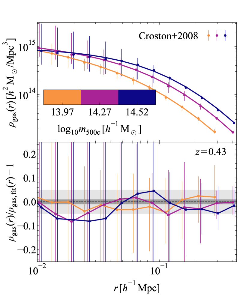
Figure 1: Top panel: The median hot gas density profiles, evolved self-similarly to $z=0.43$, with their 16th and 84th percentile scatter for the halo mass-binned density profiles from Croston et al. (2008) (coloured circles). We also show the model gas density profiles inferred from fitting the halo baryon fractions (coloured lines). Bottom panel: The ratio between the observed hot gas density profiles and our best-fitting model. We recover the observed profile at the $\approx 5\,\mathrm{per\,cent}$ level for most of the radial range, which is well within the scatter of the object-to-object scatter for individual mass bins.

To determine the baryonic component of our model, we only require a fit to the hot gas density profiles inferred from the observed X-ray surface brightness of galaxy clusters. For a detailed description of how the X-ray surface brightness is converted into the density profile, we refer to Section 3 of Debackere et al. (2020). In short, the X-ray surface brightness is fit with a spherically symmetric, collisionally ionized electron plasma of temperature $T$ and metallicity $Z$. Assuming mass abundances for hydrogen, helium and metals, we then convert the electron number density into a mass density profile. The halo masses for each cluster can then be determined from the hot gas density and temperature profiles under the assumption of hydrostatic equilibrium. We use observations from the Representative XMM-Newton Cluster Structure Survey (REXCESS, Böhringer et al. 2007) because the clusters constitute a local, high-quality, and volume-limited sample, representative of the local X-ray cluster population. Since the survey is not flux-limited, the sample suffers less from the well-known cool-core bias for X-ray cluster samples (Chon & Böhringer, 2017). However, the dynamical state of REXCESS clusters still differs from that of SZ selected samples (which suffer less from biases due to their approximate mass selection, see e.g. Rossetti et al., 2016). We evolve the inferred density profiles self-similarly to extrapolate to higher redshifts. In self-similar evolution, density profiles evolve with redshift as $\rho(z)\propto E^{2}(z)=\Omega_{\mathrm{m}}(1+z)^{3}+\Omega_{\Lambda}$ (Kaiser, 1986). Consequently, masses defined with respect to the critical density of the Universe remain constant. In the top panel of Fig. 1, we show the median of the $m_{\mathrm{500c}}$-binned observed hot gas density profiles, $\rho_{\mathrm{gas}}(r|m,z=0.43)$, evolved self-similarly to $z=0.43$ (the mean redshift of both the SPT and DES calibration samples, see Dietrich et al. 2019 and DES Collaboration et al. 2020, respectively), and the 16th and 84th percentile range from the REXCESS data of Croston et al. (2008).

Our procedure for obtaining the gas density profiles and corresponding cluster masses, relies on a couple of assumptions that we now justify. First, in linking the gas density profiles inferred from X-ray observations to the cluster masses, we have assumed hydrostatic equilibrium. This assumption implies that our resulting masses are lower limits on the true cluster masses since observations and simulations suggest that halo masses inferred from X-ray observations and hydrostatic equilibrium are underestimated by $\approx 15-30\,\mathrm{per\,cent}$ (e.g. Mahdavi et al., 2013; Von der Linden et al., 2014b; Hoekstra et al., 2015; Medezinski et al., 2018; Barnes et al., 2020; Herbonnet et al., 2020). Looking at Eq. (4), the mass ratio $m({<}r)/m_{\mathrm{dmo}}({<}r)$, whose bias we want to study, depends inversely on the inferred dark matter fraction at $r$, $1-f_{\mathrm{bar}}(r)$. If the observed cluster were not in hydrostatic equilibrium, the fixed overdensity radius would increase along with the halo mass. If the halo baryon fraction increases with radius outside $r_{\mathrm{500c}}$ (which is a valid assumption, see e.g. Vikhlinin et al. 2006), the resulting enclosed baryon fraction would be higher than the one derived assuming hydrostatic equilibrium. In this case, the true mass ratio between the observed halo and its corresponding DMO halo, $m({<}r)/m_{\mathrm{dmo}}({<}r)$, would be lower than our value inferred assuming hydrostatic equilibrium. Hence, our model provides an upper bound to the minimum possible mass ratio bias in Eq. (4) due to missing baryons.

Second, we have assumed that the hot gas density profiles evolve self-similarly with redshift. There is observational evidence that the redshift scaling of the cluster hot outer gas density profile is indeed close to self-similar (e.g. McDonald et al., 2017).

2.3 Fitting the gas density profiles

In Debackere et al. (2020), we constructed halo density profiles by fitting beta profiles to the galaxy cluster gas density profiles inferred from the observed X-ray emission. While this is certainly a valid approach, we take a different route here. In our previous work, we had to enforce steeper slopes for the observationally unconstrained outer hot gas density profile so that haloes did not exceed the cosmic baryon fraction. However, while this fine-tuning process ensures that the halo baryon fraction reaches the cosmic value at a fixed radius, it then gradually declines further out. Since we wish to ensure that the halo baryon fraction converges to the cosmic value in the halo outskirts, we decided not to fit the gas density profile, but the halo baryon fraction instead:

$$f_{\mathrm{bar}}(r|m,z)=\frac{m_{\mathrm{bar}}({<}r|m,z)}{m_{\mathrm{bar}}({<}r|m,z)+m_{\mathrm{dm}}({<}r|m,z)}\,,$$ (5)

where $m_{\mathrm{bar}}({<}r|m,z)$ and $m_{\mathrm{dm}}({<}r|m,z)$ are the enclosed baryonic and dark matter mass within $r$ for a halo of mass $m$ at redshift $z$, respectively. We can enforce the convergence to the cosmic baryon fraction in the halo outskirts by choosing a functional form for $f_{\mathrm{bar}}(r)$ that asymptotes to $\Omega_{\mathrm{b}}/\Omega_{\mathrm{m}}$.

We construct the enclosed baryon fraction profiles from the observed gas density profiles $\rho_{\mathrm{gas}}(r|m,z)$ from the REXCESS data of Croston et al. (2008). For each cluster, we determine the dark matter mass at $r_{\mathrm{500c}}$ using Eq. (2) and the NFW scale radius by solving Eq. (4), assuming the hot gas accounts for all the halo baryons. Then, we obtain $f_{\mathrm{bar}}(r|m,z)$ from Eq. (5). We show the halo baryon fraction inferred from the observations, also evolved self-similarly to $z=0.43$, in the top panel of Fig. 2.

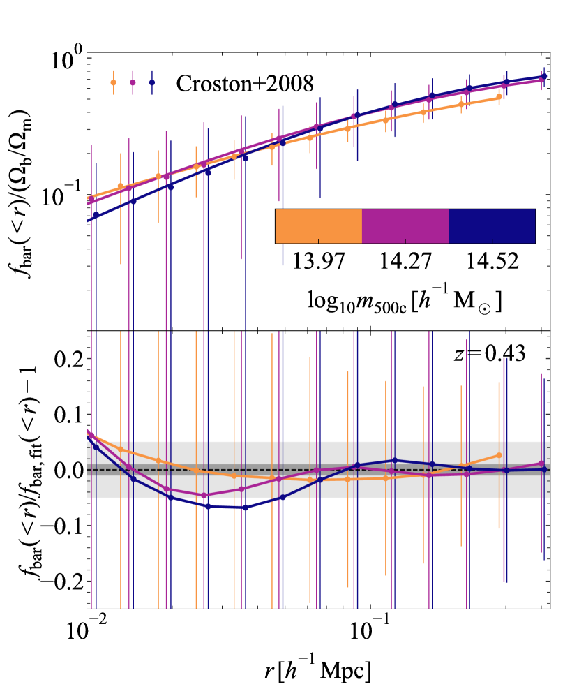
Figure 2: Top panel: The enclosed baryon fraction as a function of radius for the median, mass-binned hot gas density profiles, evolved self-similarly to $z=0.43$, including their 16th and 84th percentile scatter from Croston et al. (2008) (coloured circles). The dark matter mass is obtained by subtracting the gas mass from the inferred total halo mass. We assume the dark matter follows an NFW profile with a scale radius determined by the equivalent DMO halo that accounts for all cosmic baryons within $r_{\mathrm{500c}}$, i.e. $m_{\mathrm{dmo}}({<}r_{\mathrm{500c}})=1/(1-\Omega_{\mathrm{b}}/\Omega_{\mathrm{m}})m_{\mathrm{dm}}({<}r_{\mathrm{500c}})$. Our best-fitting model assuming Eq. (7) is shown as the coloured lines. Bottom panel: The ratio between the inferred enclosed baryon fraction from X-ray observations and our best-fitting model. We recover the correct baryon fractions at the $\approx 5\,\mathrm{per\,cent}$ level for all radii and halo masses, which is well within the scatter of the object-to-object scatter for individual mass bins.

The baryonic density profiles can be recovered by taking the derivative of the enclosed baryonic mass profile (we drop the $m$ and $z$ dependence)

$$\rho_{\mathrm{bar}}(r) =\frac{1}{4\pi r^{2}}\frac{\mathrm{d}m_{\mathrm{bar}}({<}r)}{\mathrm{d}r}$$

$$=\frac{1}{4\pi r^{2}}\frac{\mathrm{d}}{\mathrm{d}r}\left(\frac{f_{\mathrm{bar}}(r)}{1-f_{\mathrm{bar}}(r)}m_{\mathrm{dm}}({<}r)\right)$$

$$=\frac{f_{\mathrm{bar}}^{\prime}(r)m_{\mathrm{dm}}({<}r)}{4\pi r^{2}(1-f_{\mathrm{bar}}(r))^{2}}+\frac{f_{\mathrm{bar}}(r)}{1-f_{\mathrm{bar}}(r)}\rho_{\mathrm{dm}}(r)\,,$$ (6)

where ${}^{\prime}\equiv\mathrm{d}/\mathrm{d}r$. For outer boundary conditions $\lim_{r\to\infty}f_{\mathrm{bar}}(r)=\Omega_{\mathrm{b}}/\Omega_{\mathrm{m}}$ and $\lim_{r\to\infty}f_{\mathrm{bar}}^{\prime}(r)=0$, it is clear that the baryonic density profile will follow the dark matter in the halo outskirts. In fact, the total matter profile, $\rho_{\mathrm{bar}}+\rho_{\mathrm{dm}}$, will approach the equivalent DMO halo profile, since $\rho_{\mathrm{dm}}(r)=(1-\Omega_{\mathrm{b}}/\Omega_{\mathrm{m}})\rho_{\mathrm{dmo}}(r)$. This is exactly what is found in simulations when comparing the halo-matter cross-correlation (which traces the average halo density profile for a given mass) between DMO and hydrodynamical simulations (van Daalen et al., 2014).

In this paper we will assume the baryon fraction goes to zero at small radii for simplicity. Different functional behaviours, for instance including a central increase in the baryon fraction that captures the stellar contribution, are also possible. However, we are interested in studying the change in the cluster weak lensing signal due to the inclusion of baryons. Since the lensing analysis usually excludes the central regions, and the central galaxy would only contribute $\lesssim 1\,\mathrm{per\,cent}$ of the total halo mass (see e.g. Zu & Mandelbaum, 2015), we can safely neglect its contribution. We assume the profile

$$f_{\mathrm{bar}}(r|m,z)=\frac{\Omega_{\mathrm{b}}/\Omega_{\mathrm{m}}}{2}\left(1+\tanh\left(\frac{\log_{10}r-\log_{10}r_{\mathrm{t}}(m,z)}{\alpha(m,z)}\right)\right)\,,$$ (7)

which gives

$$f_{\mathrm{bar}}^{\prime}(r|m,z)=\frac{\Omega_{\mathrm{b}}/\Omega_{\mathrm{m}}}{2\ln(10)\alpha(m,z)r}\cosh^{-2}\left(\frac{\log_{10}(r/r_{\mathrm{t}}(m,z))}{\alpha(m,z)}\right)\,,$$ (8)

where $r_{\mathrm{t}}(m,z)$ determines where the increase in the baryon fraction turns over and $\alpha(m,z)$ sets the sharpness of the turnover ($\alpha\gg 1$ is smooth, $\alpha\ll 1$ is sharp). We show the best-fitting $f_{\mathrm{bar}}(r|m,z)$ profiles to the REXCESS data, assuming Eqs. (2.3), (7), and (8), in the top panel of Fig. 2. In the bottom panel of Fig. 2, we show the ratio of our model to the observations. We are able to capture the observed behaviour at the $\approx 5\,\mathrm{per\,cent}$ level for all halo masses and over most of the radial range. This accuracy is well within the observed scatter of the individual gas density profiles. The benefit of fitting the halo baryon fraction instead of the gas density, is that the outer baryonic density automatically traces the dark matter, while accounting for all of the cosmic baryons.

To extrapolate our model beyond the observed cluster masses and redshifts, we scale the density profiles self-similarly and fit $r_{\mathrm{t}}(m,z)$ and $\alpha(m,z)$, opting for the following $(m,z)$ dependencies

$$\log_{\mathrm{10}}(r_{\mathrm{t}}/r_{\mathrm{x}})(m_{\mathrm{x}},z) =\tilde{r}(z)(\log_{\mathrm{10}}m_{\mathrm{x}}-\tilde{m}(z))$$ (9)

$$\alpha(m_{\mathrm{x}},z) =\tilde{\alpha}(z)(\log_{\mathrm{10}}m_{\mathrm{x}}-\tilde{\mu}(z))\,,$$ (10)

where $[\tilde{r}(z),\tilde{m}(z),\tilde{\alpha}(z),\tilde{\mu}(z)]$ are free fitting parameters at 10 redshift bins $z\in[0.1,2]$ (we interpolate for intermediate values of $z$) and $m_{\mathrm{x}}$ is the chosen halo mass definition, $m_{\mathrm{500c}}$ in our case. The chosen linear behaviour captures the average mass dependence of the fit parameters quite well, as we show in Appendix A.

We stress that the assumed functional form for $f_{\mathrm{bar}}(r|m,z)$ implicitly fixes the gas density profile in the halo outskirts. To account for different outer gas density profiles, we also fit the halo baryon fractions inferred from the 16th and 84th percentiles of the hot gas density profiles in Fig. 1. To ensure that these fits bracket the median profile results for all masses and redshifts, we fix $\alpha(m,z)$ to the best-fitting behaviour of the median profiles, and leave $r_{\mathrm{t}}(m,z)$ free to vary. These different profile behaviours can quantify the effect of higher and lower outer gas densities, which are difficult to constrain observationally, on the inferred halo masses from weak lensing observations.

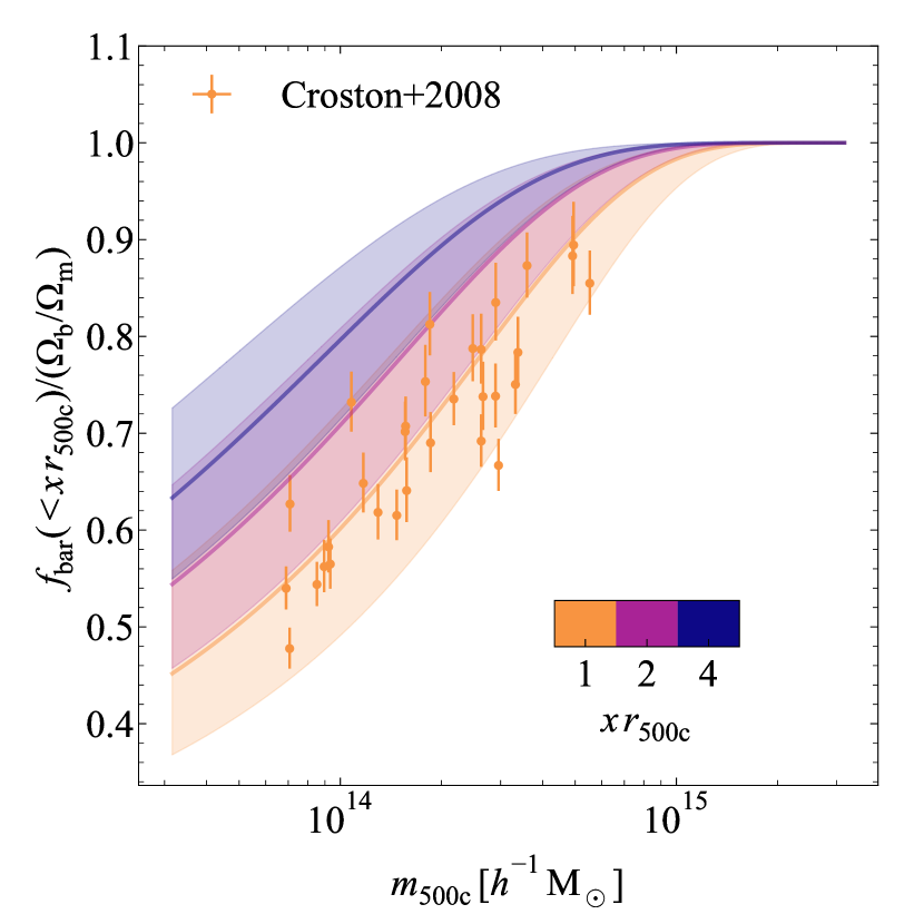
Figure 3: The REXCESS X-ray hydrostatic gas fractions as a function of halo mass from Croston et al. (2008). The median $f_{\mathrm{bar}}(<xr_{\mathrm{500c}})-m_{\mathrm{500c}}$ relations (thick, coloured lines) and the 16th to 84th percentile ranges (shaded regions) from our model fits to the inferred radial gas fractions of the observed density profiles are shown. We also show the extrapolated enclosed gas fractions at larger radii than observed.

We show the halo baryon fractions as a function of mass and for different outer radii, in Fig. 3. We also show the gas fractions at $r_{\mathrm{500c}}$ inferred from the REXCESS data. Our model closely reproduces the median behaviour. The fits to the 16th and 84th percentiles of the hot gas density profiles capture the full range of the observational uncertainty. Hence, our model is fully representative of the REXCESS galaxy cluster population.

As a consequence of our chosen functional form for the radial profile of the halo baryon fraction, Eq. (7), haloes with masses $m_{\mathrm{500c}}\gtrsim 10^{15}\,h^{-1}\,\mathrm{M_{\odot}}$ contain the cosmic baryon fraction within $r_{\mathrm{500c}}$. In simulations, however, halo baryon fractions might exceed the cosmic value at $r_{\mathrm{500c}}$ for these massive haloes since their strong potential wells prevent the ejected baryons from leaving the halo (see e.g. fig. A1 of Velliscig et al. 2014 or fig. 2 of Lee et al. 2018). The REXCESS clusters are not massive enough to observe this behaviour. Moreover, even if this were the case, the lower-mass haloes most tightly constrain the shape and normalization of the halo mass function since they are more abundant.

Another possibly important effect is that at radii larger than $r_{\mathrm{500c}}$ the hot gas pressure might prevent further infall of cosmic baryons, lowering the asymptotic baryon fraction below the cosmic value. Our mock weak lensing observations are performed at scales $\approx r_{\mathrm{500c}}$ for the most massive haloes, and should not be significantly affected by the gas distribution in the halo outskirts. Our profiles assume that the baryon fraction asymptotes to the universal fraction. If the baryon fraction at large radii were smaller than assumed, then the true halo mass, $m_{\mathrm{200m,true}}$, would be lower than our model prediction. In that case, the ratio $m_{\mathrm{200m,true}}/m_{\mathrm{200m,dmo}}$ would be smaller than what we find, since the linked DMO halo mass would remain the same. Hence, our model provides an upper limit to the true mass ratio and, consequently, a lower limit on the bias in the measured cosmological parameters from cluster counts. We stress that Eq. (5) would be able to capture these behaviours if an appropriate functional form is chosen.

In conclusion, our model accurately captures the baryonic content of the average cluster population, since we fit it to the median halo mass-binned gas density profiles inferred from cluster X-ray surface brightness profiles. This also justifies our assumption of spherical symmetry, since deviations due to the presence of substructure or triaxiality of individual haloes average out in a stacked analysis if the cluster selection is unbiased. In Section 3, we will use our model to compare the halo masses inferred from a mock weak lensing analysis to the true halo masses.

3 Mock observational analysis

Mass calibrations of observed samples of clusters are carried out for a subset of the sample for which weak lensing observations are available or follow-up observations are made (e.g. Applegate et al., 2014; Hoekstra et al., 2015; Schrabback et al., 2018; Dietrich et al., 2019). Different groups use different assumptions to derive weak lensing masses. To minimize the statistical noise in the mass determination of individual clusters due to the degeneracy between mass and concentration (see e.g. Hoekstra et al., 2011), one generally assumes a fixed concentration (as in Applegate et al. 2014 and Von der Linden et al. 2014a) or a concentration–mass relation from simulations (as in Hoekstra et al. 2015; Schrabback et al. 2018; Dietrich et al. 2019). The weak lensing derived halo masses are then used to calibrate a scaling relation between a survey observable mass proxy and the weak lensing-derived halo mass.

Using our idealized halo model described in Section 2, we can generate mock weak lensing observables for clusters with realistic baryonic density profiles. We investigate how accurately the aforementioned weak lensing derived halo mass recovers the true halo mass in the presence of baryons and how the best-fitting mass from the mock weak lensing observations compares to the mass of the same halo in a gravity-only universe, for which we can reliably predict the abundance. The mismatch between these masses determines the bias in the cosmological parameters inferred from a cluster count cosmological analysis as we will perform in Section 4.

The observable of interest for weak lensing is the reduced shear

$$g_{\mathrm{T}}(\theta)=\frac{\gamma_{\mathrm{T}}(\theta)}{1-\kappa(\theta)}\,,$$ (11)

where $\kappa(\theta)=\Sigma(\theta)/\Sigma_{\mathrm{crit}}$ is the convergence, $\gamma_{\mathrm{T}}(\theta)$ is the tangential shear, and $\Sigma_{\mathrm{crit}}$ is the critical surface mass density, defined as

$$\Sigma_{\mathrm{crit}} =\frac{c^{2}}{4\pi G}\frac{1}{\beta D_{\mathrm{l}}}\,,$$ (12)

where $D_{\mathrm{l}}$ and $\beta=\mathrm{max}(0,D_{\mathrm{ls}}/D_{\mathrm{s}})$ are the angular diameter distance between the observer and the lens, and the lensing efficiency for a source at a distance $D_{\mathrm{s}}$ from the observer and a distance $D_{\mathrm{ls}}$ behind the lens (which is negative for sources in front of the lens), respectively.

For clusters, generally $\kappa\approx\gamma_{\mathrm{T}}\approx 0.01-0.1$ at the scales probed with weak lensing observations ($0.5\lesssim R\lesssim 5\,h^{-1}\,\mathrm{Mpc}$). Assuming a cosmological model, the angular position, $\theta$, can be converted into a projected physical distance, $R$, using the observed angular diameter distance, $D$, as $\theta=R/D$. The tangential shear is given by

$$\gamma_{\mathrm{T}}(R|m,z)=\frac{\bar{\Sigma}({<}R|m,z)-\Sigma(R|m,z)}{\Sigma_{\mathrm{crit}}}\,,$$ (13)

where $\Sigma(R|m,z)$ is the projected surface mass density profile for a halo with mass $m$ at redshift $z$,

$$\Sigma(R|m,z) =\int_{-\infty}^{\infty}\rho(R,l|m,z)\mathrm{d}l$$

$$=2\int_{R}^{\infty}\mathrm{d}r\,\rho(r|m,z)\frac{r}{\sqrt{r^{2}-R^{2}}}\,,$$ (14)

which we compute with a Gauss-Jacobi quadrature to ensure convergence in the presence of the singularity at $r=R$, and $\bar{\Sigma}({<}R|m,z)$ is the mean enclosed surface mass density inside $R$

$$\bar{\Sigma}({<}R|m,z)=\frac{2}{R^{2}}\int_{0}^{R}\mathrm{d}R^{\prime}\,R^{\prime}\Sigma(R^{\prime}|m,z)\,.$$ (15)

The halo model described in Section 2 enters in Eqs. (3) and (15) through the total density profile

$$\rho(r|m,z)=\rho_{\mathrm{dm}}(r|m,z)+\rho_{\mathrm{bar}}(r|m,z)\,.$$ (16)

Here, we obtain the normalization of the dark matter NFW density profile, $\rho_{\mathrm{dm}}$, by taking the halo mass at $r_{\mathrm{500c}}$ and correcting it for the gas fraction inferred from observations of the X-ray surface brightness profiles of the REXCESS clusters (Eq. 2). We assume that the dark matter has the same NFW scale radius as the equivalent DMO halo, which can be derived by combining Eqs. (1) and (3). The baryonic density profile, $\rho_{\mathrm{bar}}$, is obtained by fitting Eq. (7) to the radial baryon fraction profiles inferred from observations.

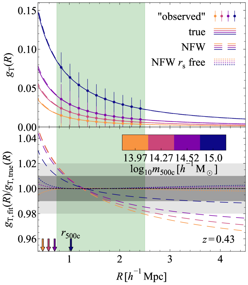
Figure 4: Top panel: The reduced shear profiles for different halo mass bins (different colours) at $z=0.43$. The mock observations with uncertainties for a single halo set by an intrinsic galaxy shape noise of $\sigma_{\mathrm{gal}}=0.25$ and mean background galaxy density of $\bar{n}=10\,\mathrm{arcmin^{-2}}$ are shown on top of the underlying true density profile (coloured dots and solid lines). The green shaded region indicates the fitting range for the mock weak lensing observations. The coloured arrows in the bottom panel indicate $r_{\mathrm{500c}}$ for the different halo mass bins. The best-fitting NFW profiles with fixed (free) scale radius, $r_{\mathrm{s}}$, are also shown as dashed lines (dotted lines). Bottom panel: The ratio of the best-fitting NFW profiles to the true profiles. Leaving the NFW scale radius free results in accurate fits to the true profiles. Fixing the scale radius to a concentration–mass relation for DMO haloes overestimates the signal in the core, where baryons are missing, and underestimates the signal in the outskirts. The mismatch decreases with increasing halo mass as more massive haloes have higher baryon fractions within the fitting range.

We show the reduced shear profiles for different halo mass bins in the top panel of Fig. 4. We have assumed a mean lensing efficiency $\langle\beta\rangle=0.5$ in Eq. (12) (in agreement with the SPT calibration sample; Dietrich et al. 2019) to generate observations in 10 radial bins between $0.75\,h^{-1}\,\mathrm{Mpc}$ and $2.5\,h^{-1}\,\mathrm{Mpc}$ at $z=0.43$, (similar to the mean redshift of the calibration samples for SPT and DES, $\langle z\rangle=0.42$ and $\langle z\rangle=0.45$, respectively; Dietrich et al. 2019; DES Collaboration et al. 2020). The observational uncertainty in the reduced shear due to the intrinsic galaxy shape noise for each bin $R_{i}$ with bin size $\Delta R_{i}$ decreases with the total number of galaxies in the bin, and is taken to be

$$\sigma_{\mathrm{obs}}^{2}=\frac{\sigma_{\mathrm{gal}}^{2}}{2\pi\bar{n}R_{i}\Delta R_{i}}\,,$$ (17)

with the intrinsic galaxy shape noise $\sigma_{\mathrm{gal}}=0.25$ (e.g. Hoekstra et al., 2000), and the mean background galaxy number density $\bar{n}=10\,\mathrm{arcmin^{-2}}$ (similar to Dietrich et al., 2019). In a stacked analysis the shape noise would decrease by a factor of $\sqrt{N}$, where $N$ is the number of clusters in the stack. However, this would not affect our best-fitting models since we do not include scatter in the mock observational data. Our mock observations are overly optimistic in this sense. However, given enough clusters, the derived mass–observable relation should converge to the one we find. We choose radial bins within the range $0.75<R_{i}/(h^{-1}\,\mathrm{Mpc})<2.5$ corresponding to angular sizes $3.2<\theta/\mathrm{arcmin}<10.7$ at $z=0.43$ for a Planck Collaboration et al. (2020) cosmology (similar to Dietrich et al., 2019). The inner radius corresponds to $\approx 1.6\,(0.5)\,r_{\mathrm{500c}}(z=0.43)$ for haloes of masses $m_{\mathrm{500c}}=10^{14}\,(10^{15.5})\,h^{-1}\,\mathrm{M_{\odot}}$. At smaller scales, cluster miscentring and contamination become important. At larger scales, the large-scale structure contributions to the surface mass density become important. For different redshifts, we scale the radial range of the observations by $(1+z)^{-1}$, i.e. $R_{i}(z)=1.43/(1+z)R_{i}(z=0.43)$, to ensure that we are not greatly exceeding $r_{\mathrm{500c}}(z)$ in the fitting range.

The dashed lines in Fig. 4 indicate the best-fitting NFW profile to the observed data points, assuming the median Correa et al. (2015) concentration–mass relation. We also show the resulting NFW profile when leaving the scale radius, $r_{\mathrm{s}}$, free as the dotted lines. Observationally, they would be difficult to distinguish from the true profile because the difference due to baryons is negligible compared to the shape noise of an individual cluster. The lower panel of Fig. 4 shows the ratio between the best-fitting NFW reduced shear profiles and the true profiles. Clearly, with currently attainable source background densities, we cannot discern the true reduced shear profile from the best-fitting NFW profiles, which would require $\mathrm{per\,cent}$ level precision for the shear measurements. We have checked that even a stage IV-like survey with $\bar{n}=30\,\mathrm{arcmin^{-2}}$ could only observe the difference between the true density profile and the NFW fit with fixed concentration–mass relation at the $\approx 2\,\sigma$ level in a stack of $\mathcal{O}(10^{4})$ clusters with $m_{\mathrm{500c}}>10^{14}h^{-1}\,\mathrm{M_{\odot}}$.

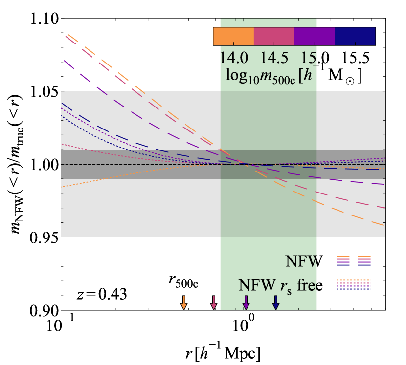
Figure 5: The ratio of the 3D enclosed total mass recovered from the best-fitting NFW profiles to the reduced shear with fixed and free scale radius, $r_{\mathrm{s}}$, to the true mass profile (dashed and dotted lines, respectively) for haloes of different masses at $z=0.43$. The green, shaded region indicates the radial range for the fit. The overdensity radii $r_{\mathrm{500c}}$ corresponding to the true density profiles are indicated with arrows. Fixing the concentration–mass relation of the NFW profile consistently overestimates (underestimates) the inner (outer) halo mass, where the baryonic mass is lower (higher) than the NFW prediction. Leaving the concentration of the NFW profile free removes the underestimation of the outer halo mass.

We obtain deprojected enclosed total halo mass profiles $m_{\mathrm{NFW}}({<}r)$ from the best-fitting NFW density profiles to the reduced shear. We show the ratio between the NFW reconstructed enclosed halo mass with fixed and free scale radius, $r_{\mathrm{s}}$, and the true halo mass in Fig. 5 for haloes with masses $m_{\mathrm{500c}}=10^{14},10^{14.5},10^{15},10^{15.5}\,h^{-1}\,\mathrm{M_{\odot}}$. The results of both fitting methods are generally within $\approx 5\,\mathrm{per\,cent}$ of the true enclosed mass profiles for all halo masses we show. However, fixing the concentration–mass relation of the NFW density results in substantially more biased halo mass estimates. The best-fitting NFW profile is determined by the fitting range of the observations and minimizes the $\chi^{2}$ error by balancing the over- and underestimation of the true profile, as can be seen in the bottom panel of Fig. 4. Since feedback processes redistribute the baryons to larger scales, the best-fitting NFW profiles consistently overestimate the halo mass internal to the minimum radius of the fit. Moreover, since the NFW profile cannot capture the more rapidly increasing baryonic mass towards the halo outskirts, the outer halo mass is consistently underestimated. This behaviour is general: the inner radius of the observational fitting range approximately determines the physical scale at which the inferred total deprojected halo masses are unbiased. For radii progressively smaller (larger) than the inner fitting radius, total deprojected masses are overestimated (underestimated) with increasing amplitude.

This bias can be reduced, however, by leaving the NFW scale radius as a free parameter. The inner halo mass will still be biased, but the extra freedom allows for practically unbiased outer halo mass estimates (see Fig. 5). This behaviour is clearly visible in the top panel of Fig. 6, where we show the ratio $m_{\mathrm{200m,NFW}}/m_{\mathrm{200m,true}}$ for both fitting methods. The bottom panel of Fig. 6 shows how $r_{\mathrm{s}}$ needs to increase with respect to the true value to capture the less centrally concentrated halo baryons. However, this is not possible when fixing the concentration–mass relation, resulting in overestimated (underestimated) masses when $r_{\mathrm{200m,true}}\lesssim(\gtrsim)1\,h^{-1}\,\mathrm{Mpc}$ (at $\approx 1\,h^{-1}\,\mathrm{Mpc}$ and $z=0.43$, the enclosed mass estimates are unbiased for our chosen fitting range, this corresponds to $m_{\mathrm{500c}}\approx 10^{14.1}\,h^{-1}\,\mathrm{M_{\odot}}$).

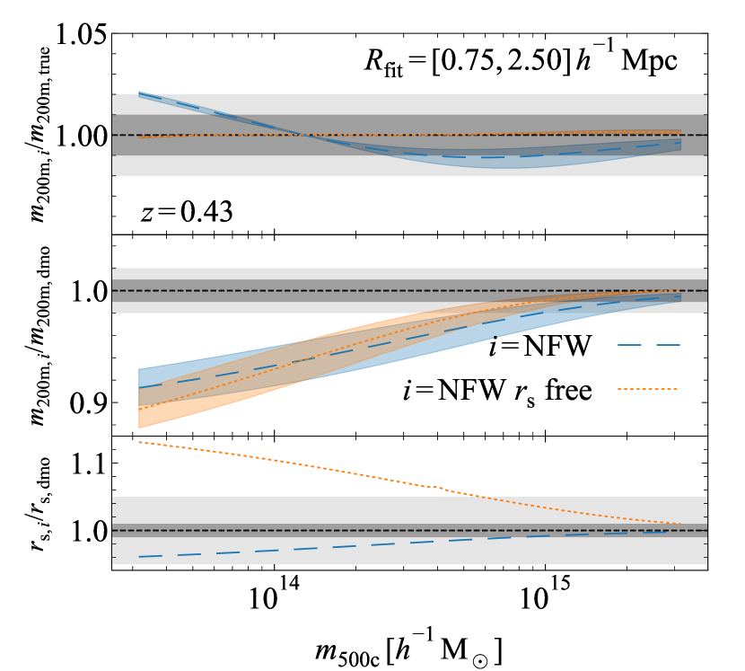
Figure 6: Top panel: The ratio of the 3D enclosed total overdensity mass, $m_{\mathrm{200m,NFW}}$, inferred from the best-fitting NFW profiles to the reduced shear, to the true halo mass $m_{\mathrm{200m,true}}$ as a function of $m_{\mathrm{500c}}$. The dashed and dotted lines show the mass ratio $m_{\mathrm{200m,NFW}}/m_{\mathrm{200m,true}}$ for the best-fitting NFW density profiles with fixed and free scale radius for a fitting range of $R_{\mathrm{fit}}=[0.75-2.5]\,h^{-1}\,\mathrm{Mpc}$, respectively. Fixing the scale radius results in biased estimates for $m_{\mathrm{200m,true}}$, leaving the scale radius free removes this bias. Middle panel: The ratio of the inferred halo mass $m_{\mathrm{200m,NFW}}$ to the equivalent dark matter-only halo mass $m_{\mathrm{200m,dmo}}$ as a function of $m_{\mathrm{500c}}$. The resulting mass ratios are biased for both mass determination methods, since the missing halo baryons bias $m_{\mathrm{200m,true}}$ with respect to $m_{\mathrm{200m,dmo}}$. Bottom panel: The ratio of the scale radius of the best-fitting NFW profile to the true dark matter-only NFW scale radius $r_{\mathrm{s,dmo}}$. Leaving the scale radius free results in larger values, since the baryons are less centrally concentrated than the dark matter.

The halo mass $m_{\mathrm{200m,NFW}}$ from the best-fitting NFW density profile can be used to obtain unbiased estimates of the true halo mass $m_{\mathrm{200m,true}}$ if the concentration–mass relation is left free. However, for cluster abundance studies, the mass of interest is not $m_{\mathrm{200m,true}}$ of the observed halo, but the halo mass of the equivalent DMO halo, $m_{\mathrm{200m,dmo}}$. All calibrated fitting functions and emulators of the halo mass function are obtained from DMO simulations (e.g. Tinker et al., 2008; McClintock et al., 2019b; Nishimichi et al., 2019; Bocquet et al., 2020), since the matter distribution in hydrodynamical simulations depends sensitively on the assumed “subgrid” physics recipes required to model the complex galaxy formation processes (e.g. Velliscig et al., 2014).

We show the ratio $m_{\mathrm{200m,NFW}}/m_{\mathrm{200m,dmo}}$ as a function of halo mass $m_{\mathrm{500c}}$ in the middle panel of Fig. 6. We do not show the ratio $m_{\mathrm{200m,true}}/m_{\mathrm{200m,dmo}}$ for the actual halo mass since it matches the relation for the best-fitting NFW density profile with a free scale radius (shown as the dotted line) almost exactly (the halo mass $m_{\mathrm{200m,NFW}}$ is nearly unbiased when the NFW scale radius is left free). The suppression of the true halo mass with respect to the equivalent DMO halo stems from the missing halo baryons within $r_{\mathrm{200m,true}}$. Fixing the concentration–mass relation of the NFW density profile (shown as the dashed line) results in biases similar to leaving the NFW scale radius free, except for the small modulation due to the mass bias in $m_{\mathrm{200m,NFW}}$ with respect to $m_{\mathrm{200m,true}}$ (see the top panel of Fig. 6). As mentioned earlier, this bias stems from the chosen radial fitting range for the weak lensing observations. Decreasing (increasing) the inner fitting radius shifts the crossover between over- and underestimated $m_{\mathrm{200m,true}}$ to lower (higher) halo masses and changes the overall amplitude of the bias. Remarkably, for low-mass haloes ($m_{\mathrm{500c}}\lesssim 10^{14.1}\,h^{-1}\,\mathrm{M_{\odot}}$), the overestimation of $m_{\mathrm{200m,true}}$ when fixing the concentration–mass relation results in a less biased estimate of $m_{\mathrm{200m,dmo}}$. However, we would preferably not rely on more biased estimates of the true halo mass to obtain less biased cosmological parameters.

We find a slightly stronger suppression in the ratio $m_{\mathrm{200m,true}}/m_{\mathrm{200m,dmo}}$ in our model compared to cosmo-OWLS (for $r_{\mathrm{s}}$ free we find $>1\,\mathrm{per\,cent}$ suppression for $m_{\mathrm{500c}}\lesssim 10^{15}\,h^{-1}\,\mathrm{M_{\odot}}$ compared to $m_{\mathrm{500c}}\lesssim 10^{14.5}\,h^{-1}\,\mathrm{M_{\odot}}$ in Velliscig et al. 2014). The reason for this is twofold. First, we do not include a stellar component in our model. Since stars are more centrally concentrated than the hot gas, the NFW fits in cosmo-OWLS perform slightly better in the inner regions, capturing an extra $\approx 1\,\mathrm{per\,cent}$ of the total halo mass there and reducing the mass ratio bias. Second, in cosmo-OWLS contraction of the dark matter component due to the baryons at these halo masses slightly reduces the bias since more dark matter mass is included in the central regions than we are accounting for in Eq. (1). However, for $m_{\mathrm{500c}}\gtrsim 10^{14}\,h^{-1}\,\mathrm{M_{\odot}}$, the dark matter contraction increases the enclosed halo mass ratio $m_{\mathrm{dm}}({<}r)/m_{\mathrm{dmo}}({<}r)$ in Eq. (1) by only $\lesssim 1\,\mathrm{per\,cent}$ (see fig. 3 of Velliscig et al., 2014). For $m_{\mathrm{500c}}\lesssim 10^{14}\,h^{-1}\,\mathrm{M_{\odot}}$, the dark matter actually slightly expands, lowering the dark matter mass and increasing the bias.

We decided not to include a stellar component or dark matter contraction to keep our model simple. Moreover, when investigating the impact of the halo mass determination on the inferred cosmological parameters, lower-mass haloes with $m_{\mathrm{500c}}\lesssim 10^{14.5}\,h^{-1}\,\mathrm{M_{\odot}}$ dominate the signal since they are significantly more abundant and hence the fit is more sensitive to any bias in this mass range. At low masses, all the aforementioned effects are clearly much less important than the change in halo mass due to the missing halo gas. Hence, we conclude that our model provides a reasonable estimate of the halo mass bias induced by the change in halo density profiles due to the presence of baryons.

4 Influence on cosmological parameter estimation

In this section we will investigate how the bias in the halo masses inferred from mock weak lensing observations that we derived in Section 3, biases the measurement of cosmological parameters from a number count analysis of a mock cluster sample.

4.1 Mock cluster sample generation

We create a cluster sample by drawing $(\log_{10}m_{\mathrm{200m}},z)$ pairs from the Poisson distribution with mean number density

$$\frac{\mathrm{d}N(m,z;\mathbf{\mathscr{C}})}{\mathrm{d}\log_{10}m\,\mathrm{d}z} =\Omega_{\mathrm{survey}}\frac{\mathrm{d}V_{\mathrm{c}}(z;\mathbf{\mathscr{C}})}{\mathrm{d}z\mathrm{d}\Omega}\frac{\mathrm{d}n(m,z;\mathbf{\mathscr{C}})}{\mathrm{d}\log_{10}m\,\mathrm{d}z}\,,$$ (18)

with the halo mass function $\mathrm{d}n/\mathrm{d}\log_{10}m\,\mathrm{d}z$ of Tinker et al. (2008) and the comoving volume $V_{\mathrm{c}}(z)$ for a Planck Collaboration et al. (2020) cosmology with $\mathbf{\mathscr{C}}\equiv\{\Omega_{\mathrm{m}},\Omega_{\mathrm{b}},\Omega_{\Lambda},\sigma_{8},n_{\mathrm{s}},h\}=\{0.315,0.049,0.685,0.811,0.965,0.674\}$. The sky area, $\Omega_{\mathrm{survey}}$, depends on the specific survey. We use the CCL library to calculate the halo mass function (Chisari et al., 2019). We draw samples from the non-homogeneous Poisson distribution by thinning the homogeneous expectation on a grid of $(\log_{10}m_{\mathrm{200m}},z)$ bins following the method of Lewis & Shedler (1979).

Since the Tinker et al. (2008) mass function was calibrated on DMO simulations, the resulting mock cluster sample corresponds to a universe that contains only dark matter. As we have shown in Section 3, however, there is a mismatch between the true halo mass, $m_{\mathrm{200m,true}}$, and the mass of the equivalent DMO halo, $m_{\mathrm{200m,dmo}}$, due to the ejection of baryons (see the middle panel of Fig. 6). Moreover, the halo masses inferred from mock weak lensing observations, $m_{\mathrm{200m,NFW}}$, can be biased with respect to the true halo mass (see the top panel of Fig. 6). If these baryonic biases are not taken into account in the cluster count analysis, the measured cosmological parameters will be biased.

For each DMO halo in the cluster sample, we determine the biased halo mass estimate of the corresponding halo with baryons, $m_{\mathrm{200m,NFW}}(m_{\mathrm{200m,dmo}},z)$, inferred from the NFW fits to the mock weak lensing observations with either a fixed or free scale radius in Section 3. We interpolate the relation between the mass of the halo including baryons and the mass of its equivalent DMO halo, $m_{\mathrm{500c}}(m_{\mathrm{200m,dmo}},z)$, from our halo model and determine the corresponding mass ratio $m_{\mathrm{200m,NFW}}/m_{\mathrm{200m,dmo}}$ (see the middle panel of Fig. 6 for the ratio at $z=0.43$). We will investigate how severely this baryonic mass bias affects the measured cosmological parameters for stage III and stage IV-like surveys in Sections 4.2 and 4.3, respectively.

We start with a best-case scenario, where we have assumed a one-to-one mapping between the observable mass proxy (e.g. the SZ detection significance) and the halo masses inferred from weak lensing, i.e. we neglect the measurement uncertainties in the mass estimation of individual clusters (we consider a more realistic scenario in Sec. 4.3). This allows us to take the weak lensing inferred halo masses as the starting point of our analysis. When connecting haloes to their DMO equivalents, we also do not account for the intrinsic scatter due to the differing mass distributions of individual haloes that arise from their unique mass accretion histories. We assign the weak lensing inferred halo masses to the DMO haloes without scatter. This is consistent with our choice in Section 2.3, where we fit to the median halo mass-binned cluster population of REXCESS, neglecting differences between individual clusters in each mass bin.

Ignoring the mass estimation uncertainty and the intrinsic scatter in the halo population would bias the observable–mass relation in an observed cluster sample due to the preferential scatter of more abundant low-mass haloes into higher mass bins. Hence, in a full cosmological analysis, converting the observable to the true halo mass requires the inclusion of the mass estimation uncertainty, and the intrinsic scatter in the halo population, while accounting for the change in abundance of clusters as a function of mass and redshift. This involves a joint fit to the abundance and the observable–mass relation of the cluster sample as a function of cosmology (see e.g. Bocquet et al., 2019). In the more realistic scenario in Sec. 4.3, we will implicitly assume that the scatter is constrained by the cluster abundances, so that the precision of cosmological parameter estimation is not significantly affected by not performing such a joint analysis.

4.2 Stage III-like survey

For a stage III-like cluster survey (e.g. SPT or DES; Bocquet et al. 2019 and DES Collaboration et al. 2020, respectively), we set the survey area to $\Omega_{\mathrm{survey}}=2500\,\mathrm{deg}^{2}$ to generate the cluster sample using Eq. (18).

We want to quantify the statistical bias and uncertainty of the cosmological parameters due to the baryonic halo mass bias. Hence, we generate 1000 independent cluster samples and fit the Maximum A-posteriori Probabilities (MAPs) of the posterior distribution for each of the halo samples. We follow Cash (1979) and de Haan et al. (2016) and obtain the posterior distribution for the cosmological parameters $\mathbf{\mathscr{C}}=\{\Omega_{\mathrm{m}},\sigma_{8},w_{0}\}$ by sampling the Poisson likelihood, which is given up to a constant by

$$\ln\mathcal{L}\propto 2\left(\sum_{i}\ln\frac{\mathrm{d}N(m_{i},z_{i};\mathbf{\mathscr{C}})}{\mathrm{d}m\,\mathrm{d}z}-\int\mathrm{d}m\,\mathrm{d}z\,\frac{\mathrm{d}N(m,z;\mathbf{\mathscr{C}})}{\mathrm{d}m\,\mathrm{d}z}\right)\,,$$ (19)

where $i$ runs over the individual clusters in the sample and the integral is performed between $(z_{\mathrm{min}}=0.25,m_{\mathrm{200m,min}}=10^{14.5}\,h^{-1}\,\mathrm{M_{\odot}})$ and $(z_{\mathrm{max}}=2,m_{\mathrm{200m,max}}=10^{16}\,h^{-1}\,\mathrm{M_{\odot}})$. The lower bounds are set by the sample selection and the upper bounds are chosen high enough that the integral approaches the limit for $z,m\to\infty$. We assume flat prior distributions $\Omega_{\mathrm{m}}\sim U(0.1,0.6)$, $\sigma_{8}\sim U(0.5,1.1)$, and $w_{0}\sim U(-1.5,-0.5)$, where $U(a,b)$ indicates the uniform distribution between $a$ and $b$. We fix the remaining cosmological parameters to the assumed Planck Collaboration et al. (2020) values.

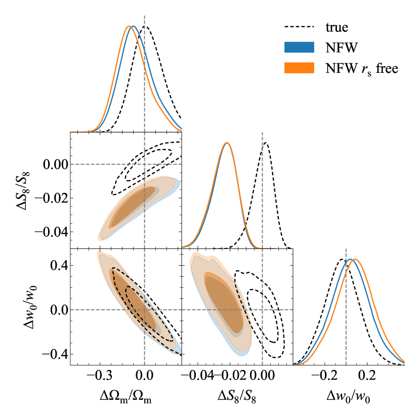
Figure 7: The distribution of the maximum a-posteriori probabilities in $(\Omega_{\mathrm{m}},S_{8}=\sigma_{8}(\Omega_{\mathrm{m}}/0.3)^{0.2},w_{0})$ for 1000 independent stage III-like cluster abundance surveys. Dashed contours show the results for a halo sample with no mass bias. Blue (orange) contours include a mass bias due to an NFW fit to mock weak lensing observations of the reduced shear, with a fixed (free) scale radius, $r_{\mathrm{s}}$. Neither $\Omega_{\mathrm{m}}$ nor $w_{0}$ are significantly biased due to baryonic effects. Relative constraints on $S_{8}$, however, are biased by $-0.023_{-0.008}^{+0.007}$ ($\approx 3\,\sigma$) for both fixed and free scale radii in the NFW fit.

We show the resulting distribution of MAPs in $(\Omega_{\mathrm{m}},S_{8}=\sigma_{8}(\Omega_{\mathrm{m}}/0.3)^{0.2},w_{0})$ for each of the different observational mass inferences in Fig. 7. The dashed contours show the unbiased halo sample. For this unbiased sample, all cosmological parameters are unbiased and we find relative uncertainties of $\approx\pm 10\,\mathrm{per\,cent}$ in $\Omega_{\mathrm{m}}$, $\approx\pm 0.7\,\mathrm{per\,cent}$ in $S_{8}$, and $\approx\pm 16\,\mathrm{per\,cent}$ in $w_{0}$ for a current stage III-like cluster survey. The quoted precision of all parameters underestimates the true uncertainty, since we have performed an idealized analysis that does not include observational uncertainties or intrinsic scatter in the derived halo masses, as mentioned before. However, as we have already shown in Fig. 6, the inferred halo masses are biased with respect to the equivalent DMO halo mass due to the missing halo baryons. Hence, NFW inferred halo masses with fixed and free scale radii (blue and orange contours, respectively) are both predominantly biased in $S_{8}$, with a median bias and 16th-84th percentile uncertainties of $\Delta S_{8}/S_{8}=-0.023_{-0.008}^{+0.007}$, where the negative value indicates that $S_{8}$ is underestimated. Neither $\Omega_{\mathrm{m}}$ nor $w_{0}$ show a significant bias for the different mass determination methods. We list the cosmological parameter constraints for both methods in Table 1.

Table 1: Inferred median bias and 16th-84th percentile statistical uncertainties of the individual best-fitting cosmological parameters for the different mass determination for a stage III-like survey with survey area $\Omega_{\mathrm{survey}}=2500\,\mathrm{deg}^{2}$ and limiting redshift and halo mass $(z_{\mathrm{min}}=0.25,z_{\mathrm{max}}=2,m_{\mathrm{200m,min}}=10^{14.5}\,h^{-1}\,\mathrm{M_{\odot}})$. The columns correspond to cosmological parameters inferred from cluster samples with halo masses inferred from weak lensing fits with (a) fixed and (b) free NFW scale radii, and (c) the true cluster masses.

	(a)NFW $r_{\mathrm{s}}$ fixed	(b)NFW $r_{\mathrm{s}}$ free	(c)true
$\Delta\Omega_{\mathrm{m}}/\Omega_{\mathrm{m}}$	$-0.06_{-0.10}^{+0.12}$	$-0.09_{-0.09}^{+0.11}$	$0.02_{-0.10}^{+0.11}$
$\Delta S_{8}/S_{8}$	$-0.023_{-0.008}^{+0.007}$	$-0.023_{-0.008}^{+0.007}$	$0.001_{-0.007}^{+0.005}$
$\Delta w_{0}/w_{0}$	$0.02_{-0.16}^{+0.19}$	$0.09_{-0.18}^{+0.18}$	$-0.03_{-0.16}^{+0.16}$

The shifts in the cosmological parameters can be understood in the following way. At a given redshift and for a fixed number count, the mass bias results in an underestimation of the true halo mass. Hence, the number of clusters assigned to the inferred halo mass is lower than it should be, since the number density of clusters increases with decreasing mass. This underestimation is then explained by decreasing the amount of structure in the Universe, assuming that we are unaware of any mass bias.

In summary, current stage III-like cluster abundance surveys with ideal mass estimations would find a biased cosmology (mainly in $S_{8}$) due to the mismatch between $m_{\mathrm{200m,true}}$ and $m_{\mathrm{200m,dmo}}$. However, due to the uncertainties induced by the mass estimation, which are larger than the statistical uncertainty of our idealized survey, the baryonic mass bias is currently not highly significant. As a reference, the current quoted uncertainties for SPT (DES; Bocquet et al. 2019 and DES Collaboration et al. 2020, respectively) are $\pm 17\,(17)\,\mathrm{per\,cent}$ in $\Omega_{\mathrm{m}}$, $\pm 3\,(6)\,\mathrm{per\,cent}$ in $S_{8}$ (with $S_{8}$ definitions differing from ours for both SPT and DES), and $\pm 26\,(-)\,\mathrm{per\,cent}$ in $w_{0}$ (DES does not constrain $w_{0}$), respectively. These values exceed our statistical uncertainties of $\pm 10\,\mathrm{per\,cent}$, $\pm 0.7\,\mathrm{per\,cent}$ and $\pm 16\,\mathrm{per\,cent}$, respectively. The baryonic bias in the cosmological parameters that our model predicts corresponds to a statistical significance of $0.5\,\sigma$ ($0.5\,\sigma$) in $\Omega_{\mathrm{m}}$, $0.8\,\sigma$ ($0.4\,\sigma$) in $S_{8}$, $0.3\,\sigma$ ($-$) in $w_{0}$ for the precision of SPT (DES). In Sec. 4.3, we show that the precision of the inferred cosmological parameters is set by the accuracy with which the uncertainty in the mass estimation is known. The mass estimation uncertainty is strongly degenerate with $S_{8}$ and imposing an uninformative prior on the uncertainty of individual cluster masses results in a significant decrease in the precision of the constraint on $S_{8}$, in line with the comparison to SPT and DES.

4.3 Stage IV-like survey

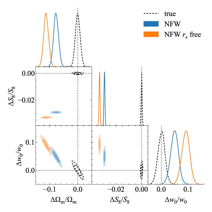
Figure 8: The distribution of the maximum a-posteriori probabilities in $(\Omega_{\mathrm{m}},S_{8}=\sigma_{8}(\Omega_{\mathrm{m}}/0.3)^{0.2},w_{0})$ for 1000 independent stage IV-like cluster abundance surveys. Dashed contours show the results for a halo sample with no mass bias. Blue (orange) contours include a mass bias due to an NFW fit to mock weak lensing observations of the reduced shear, with a fixed (free) scale radius, $r_{\mathrm{s}}$. Relative constraints on $S_{8}$ are very highly biased for both NFW fitting methods to the cluster density profiles including baryons. Similarly, $\Omega_{\mathrm{m}}$ and $w_{0}$ are biased by up to $13\,\sigma$ and $6\,\sigma$, respectively.

For a stage IV-like survey such as Euclid, the survey area increases dramatically to $\Omega_{\mathrm{survey}}=15000\,\deg^{2}$. These surveys will generally rely on observed galaxy overdensities to detect clusters and will, consequently, have more complex selection functions that depend on the magnitude limit of the survey (see e.g. Sartoris et al., 2016). We take a simple mass cut of $m_{\mathrm{200m,min}}=10^{14}\,h^{-1}\,\mathrm{M_{\odot}}$ and redshift cuts of $z_{\mathrm{min}}=0.1$ and $z_{\mathrm{max}}=2$. Due to the increase in survey area and the decrease in $m_{\mathrm{200m,min}}$, the total number of clusters increases by about two orders of magnitude compared with a stage III-like survey. The Poisson likelihood in Eq. (19) becomes intractable, especially if different mass calibrations are to be included, such as in de Haan et al. (2016). We therefore switch to the Gaussian likelihood for bins where the number of observed clusters, $N_{\mathrm{obs}}(m_{i},z_{j})>10$

$$\ln\mathcal{L}\propto\sum_{m_{i},z_{j}} -\frac{(N_{\mathrm{obs}}(m_{i},z_{j})-N(m_{i},z_{j};\mathscr{C}))^{2}}{2N(m_{i},z_{j};\mathscr{C})}$$ (20)

$$-\frac{\ln N(m_{i},z_{j};\mathscr{C})}{2}\,,$$

and we use the Poisson likelihood for the other bins

$$\ln\mathcal{L}\propto\sum_{m_{i},z_{j}} N_{\mathrm{obs}}(m_{i},z_{j})\ln N(m_{i},z_{j};\mathscr{C})-N(m_{i},z_{j};\mathscr{C})$$ (21)

$$-\ln N_{\mathrm{obs}}(m_{i},z_{j})!\,,$$

where $(m_{i},z_{j})$ run over the logarithmic bins in $m_{\mathrm{200m}}$ and the linear bins in $z$, respectively. We transition at the value $N_{\mathrm{obs}}(m_{i},z_{j})=10$ since Eq. (20) is biased with respect to Eq. (21) by a factor of $1+O(N_{\mathrm{obs}}^{-1/2})$, as worked out by Cash (1979). The Gaussian likelihood makes it easier to include contributions from the sample variance, which will also need to be included for the lower-mass haloes probed by stage IV-like surveys (Hu & Kravtsov, 2003). We have neglected the sample covariance in generating our halo sample and, hence, we do not include it in our likelihood analysis. We include the Poisson likelihood for the bins with low number counts since the Gaussian likelihood cannot properly account for the discreteness of the number count data, biasing the cosmological parameter estimates, as we show in Appendix B. In a more realistic setting, the sample variance should be included in the cluster catalogue generation and the cluster number count analysis. For stage IV-like surveys with low limiting masses, the sample variance can dominate the shot noise, increasing the uncertainty on the cluster number density, which reduces the bias for the bins with low number counts. We choose 40 equally spaced bins between $\log_{10}m_{\mathrm{200m,min}}/(h^{-1}\,\mathrm{M_{\odot}})=14.0$ and the highest halo mass present in each cluster sample. For the redshift, we take 8 equally spaced bins for $z\in[0.1,2]$. We assume the same priors as we did in Section 4.2.

We show the resulting distribution of MAPs for the stage IV-like survey in Fig. 8. The relative uncertainties for the unbiased sample shrink to $\approx\pm 1.0\,\mathrm{per\,cent}$ in $\Omega_{\mathrm{m}}$, $\approx\pm 0.04\,\mathrm{per\,cent}$ in $S_{8}$, and $\approx\pm 1.5\,\mathrm{per\,cent}$ in $w_{0}$ for a stage IV-like cluster survey. Again, we stress that we underestimate the true uncertainty, since we do not include any mass calibration uncertainties. However, in our idealized analysis, the bias from ignoring baryonic effects in the NFW inferred halo masses becomes catastrophic for $S_{8}$, both for fixed and free scale radii. Moreover, we also find very significant biases of up to $13\,\sigma$ in $\Omega_{\mathrm{m}}$ and up to $6\,\sigma$ in $w_{0}$ (for the exact values, see Table 2).

Table 2: Inferred median bias and 16th-84th percentile statistical uncertainties of the individual best-fitting cosmological parameters for the different mass determination methods for a stage IV-like survey with $\Omega_{\mathrm{survey}}=15000\,\mathrm{deg}^{2}$ and $(z_{\mathrm{min}}=0.1,z_{\mathrm{max}}=2,m_{\mathrm{200m,min}}=10^{14}\,h^{-1}\,\mathrm{M_{\odot}})$. The rows show cosmological parameters inferred from cluster samples with halo masses inferred from weak lensing fits with fixed or free NFW scale radii, and the true cluster masses. The columns show the results for samples with (a) ideal mass determinations, a mass uncertainty of $\pm 20\,\mathrm{per\,cent}$ either (b) marginalized over $\sigma_{\ln m}\sim N(\ln 1.2,\ln 1.02)$, or (c) included with a uniform prior $\sigma_{\ln m}\sim U(\ln 1.001,\ln 2)$ in the cosmological parameter estimation.

Mass uncertainty [$\mathrm{per\,cent}$]		(a)ideal [$0$]	(b)marg. [$\pm 20$]	(c)uniform [$\pm 20$]
NFW $r_{\mathrm{s}}$ fixed	$\Delta\Omega_{\mathrm{m}}/\Omega_{\mathrm{m}}$	$-0.078_{-0.008}^{+0.009}$	$-0.077_{-0.008}^{+0.009}$	$-0.055_{-0.009}^{+0.010}$
	$\Delta S_{8}/S_{8}$	$-0.0291_{-0.0004}^{+0.0004}$	$-0.0297_{-0.0004}^{+0.0004}$	$-0.047_{-0.004}^{+0.004}$
	$\Delta w_{0}/w_{0}$	$0.055_{-0.015}^{+0.014}$	$0.047_{-0.014}^{+0.013}$	$0.055_{-0.014}^{+0.013}$
NFW $r_{\mathrm{s}}$ free	$\Delta\Omega_{\mathrm{m}}/\Omega_{\mathrm{m}}$	$-0.113_{-0.008}^{+0.009}$	$-0.112_{-0.009}^{+0.009}$	$-0.076_{-0.009}^{+0.010}$
	$\Delta S_{8}/S_{8}$	$-0.0329_{-0.0004}^{+0.0004}$	$-0.0337_{-0.0004}^{+0.0004}$	$-0.066_{-0.004}^{+0.004}$
	$\Delta w_{0}/w_{0}$	$0.091_{-0.015}^{+0.014}$	$0.089_{-0.015}^{+0.014}$	$0.100_{-0.016}^{+0.014}$
true	$\Delta\Omega_{\mathrm{m}}/\Omega_{\mathrm{m}}$	$-0.0_{-0.008}^{+0.009}$	$-0.001_{-0.008}^{+0.009}$	$0.003_{-0.008}^{+0.010}$
	$\Delta S_{8}/S_{8}$	$0.0_{-0.0004}^{+0.0003}$	$-0.0002_{-0.0004}^{+0.0004}$	$0.001_{-0.003}^{+0.003}$
	$\Delta w_{0}/w_{0}$	$0.001_{-0.014}^{+0.011}$	$0.002_{-0.013}^{+0.012}$	$0.002_{-0.013}^{+0.012}$

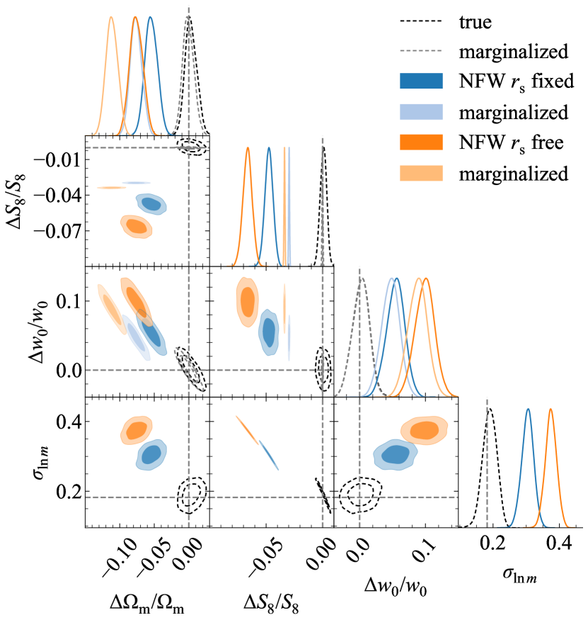
Figure 9: The marginalized maximum a-posteriori probability density functions for $\Omega_{\mathrm{m}}$, $S_{8}=\sigma_{8}(\Omega_{\mathrm{m}}/0.3)^{0.2}$, $w_{0}$, and $\sigma_{\ln m}$ for 1000 independent stage IV-like cluster abundance surveys with an uncertainty of $\pm 20\,\mathrm{per\,cent}$ on the individual cluster masses, assuming a mixed Gaussian-Poisson likelihood. Dashed contours show the results for a halo sample with no mass bias. Blue (orange) contours include a mass bias due to an NFW fit to mock weak lensing observations of the reduced shear, with a fixed (free) scale radius, $r_{\mathrm{s}}$. Dark contours also sample the individual cluster mass uncertainty $\sigma_{\ln m}$, whereas light contours have marginalized over a Gaussian distribution $\sigma_{\ln m}\sim N(\ln 1.2,\ln 1.02)$. Due to the preferential scatter of low-mass haloes into higher mass bins, an underestimate (overestimate) of $\sigma_{\ln m}$ for a fixed true value of $\sigma_{\ln m}=\ln 1.02$, results in an overestimate (underestimate) of $S_{8}$. Marginalizing over the mass uncertainty recovers the constraints obtained without mass uncertainty nearly identically.

However, the statistical precision of the cosmological parameters is overly optimistic since we neglect any uncertainty on the individual cluster masses inferred, resulting in extremely significant biases due to baryonic effects. For stage IV-like surveys, the amplitude of the mean observable–mass relation can reach $\mathrm{per\,cent}$ level accuracy due to the large number of clusters detected (see e.g. Köhlinger et al., 2015). However, the mass of an individual cluster derived from the survey observable mass proxy will still have an uncertainty. For an observable with a scatter of $\pm 20\,\mathrm{per\,cent}$ in the distribution $P(m|\mathcal{O})$ of the true total halo mass, $m$, given the observable, $\mathcal{O}$ (similarly to the richness, see e.g. Rykoff & Rozo, 2014; Mantz et al., 2016; Sereno et al., 2020), we expect an uncertainty of $\pm 20\,\mathrm{per\,cent}$ on the inferred masses of an unbiased cluster sample.

In our idealized setting, we know the true underlying halo masses. We mimic the uncertainty by adding a log-normal scatter of $\pm 20\,\mathrm{per\,cent}$ to the true halo masses of the unbiased cluster samples and to the weak lensing inferred halo masses of the biased cluster samples. We modify Eq. (18) to include an unknown mass uncertainty $\sigma_{\log_{10}m}$ for each mass bin $i$, following Lima & Hu (2005)

$$\frac{\mathrm{d}N_{i}(m,z;\mathbf{\mathscr{C}})}{\mathrm{d}\log_{10}m\,\mathrm{d}z}=\frac{1}{2}\frac{\mathrm{d}N(m,z;\mathbf{\mathscr{C}})}{\mathrm{d}\log_{10}m\,\mathrm{d}z}(\mathrm{erfc}(x_{i})-\mathrm{erfc}(x_{i+1})),$$ (22)

where

$$x_{i}=\frac{\log_{10}m^{\mathrm{obs}}_{i}-\log_{10}m}{\sqrt{2\sigma^{2}_{\log_{10}m}}}\,,$$ (23)

with $i$ and $i+1$ the edges of mass bin $i$. Adding the observational uncertainty will result in haloes scattering to different mass bins, with each bin gaining relatively more low-mass haloes due to their higher abundance. We assume a uniform distribution for the mass uncertainty with $\sigma_{\log_{10}m}\sim U(\log_{10}1.001,\log_{10}2)$. In practice, we will have some prior knowledge of the mass uncertainty of individual clusters. We quantify this effect by including a cosmological analysis with a marginalization over the mass uncertainty distribution $\sigma_{\log_{10}m}\sim N(\log_{10}1.2,\log_{10}1.02)$, corresponding to the case where the mass uncertainty is known to within $2\,\mathrm{per\,cent}$.

We show the resulting MAPs for the 1000 cluster samples with both an uninformative prior (dark contours) and a marginalization (light contours) over the individual cluster mass uncertainty in Fig. 9. For the former case, we show the posterior constraints on $\sigma_{\ln m}$ (which equals $\sigma_{\log_{10}m}/\log_{10}e$, and approximately corresponds to the $\mathrm{per\,cent}$ error on the halo mass). In the uninformative case, the mass uncertainty is strongly degenerate with $S_{8}$, since an overestimate (underestimate) of the true uncertainty would result in more (less) haloes predicted to scatter into higher mass bins. At fixed observed number count $N(m_{i},z_{j})$, this effect is compensated by decreasing (increasing) $S_{8}$.

Compared to cluster samples with unbiased masses and no mass estimation uncertainty, we find that the figure of merit (which we take as the inverse of the area enclosed by $95\,\mathrm{per\,cent}$ of the surveys) for cluster samples with unbiased masses and no prior knowledge of the cluster mass uncertainty of $\pm 20\,\mathrm{per\,cent}$ (dark, dashed contours), decreases by factors of 7.1, 1.4, and 7.6 in the $(\Omega_{\mathrm{m}},S_{8})$, $(\Omega_{\mathrm{m}},w_{0})$ and $(S_{8},w_{0})$ planes, respectively. Similarly, the 1D marginalized regions containing $68\,\mathrm{per\,cent}$ of the surveys increase by factors of 1.05, 7.7, and 1.02 for $\Omega_{\mathrm{m}}$, $S_{8}$, and $w_{0}$, respectively. However, with accurate prior knowledge of the individual cluster mass estimation uncertainty (light, dashed contours), the inferred cosmological parameters and their precision are fully consistent with the ideal mass estimation case. This can be seen by comparing the dashed and light dashed contours from Figs. 8 and 9, respectively, or by comparing the cosmological parameter constraints in columns (a) and (b) for the true halo masses in Table 2.

We find similar results when comparing the cluster samples that include a baryonic bias and an uncertainty in the halo mass determination to samples that include the baryonic bias but no mass estimation uncertainty. In the case of the uniform prior on $\sigma_{\ln m}$ (dark, coloured contours), the figure of merit in the $(\Omega_{\mathrm{m}},S_{8})$, $(\Omega_{\mathrm{m}},w_{0})$ and $(S_{8},w_{0})$ planes for a weak lensing fit with free (fixed) NFW scale radius, decreases by factors of 11.2 (9.8), 1.7 (1.5), and 9.6 (8.9), respectively. Similarly, the 1D marginalized regions for $\Omega_{\mathrm{m}}$, $S_{8}$, and $w_{0}$ containing $68\,\mathrm{per\,cent}$ of the surveys, increase by factors of 1.1 (1.1), 10.1 (9.4), and 1 (0.9), respectively. However, if the mass uncertainty is known to within $2\,\mathrm{per\,cent}$ (light, coloured contours), then the ideal case is recovered nearly identically. This can be seen by comparing the coloured and light coloured contours from Figs. 8 and 9, respectively, or by comparing the cosmological parameter constraints in columns (a) and (b) for the NFW fits with fixed and free scale radii in Table 2. We note that the distribution of the MAPs for the cluster samples with a baryonic mass bias do not match between the informative and uninformative cases. This is because the halo number counts calculated with Eq. (22) do not account for the mass-dependent baryonic bias. Hence, when leaving the mass uncertainty as a free parameter, a more likely solution is found by significantly increasing its value from the actual uncertainty, resulting in a decrease in $S_{8}$. This does not happen for the cluster samples without a mass bias.

Any bias in the cosmological parameters can be reduced at the expense of a larger uncertainty by increasing the mass cut of the cluster sample. We show the marginalized 1D probability density functions for the cosmological parameters for cluster samples without mass uncertainties using different limiting masses in Fig. 10. Increasing the mass cut from $m_{\mathrm{200m,min}}=10^{14}\,h^{-1}\,\mathrm{M_{\odot}}$ to $m_{\mathrm{200m,min}}=10^{14.5}\,h^{-1}\,\mathrm{M_{\odot}}$ reduces the bias in $S_{8}$ by a factor $\approx 8$ to $10\,\sigma$, while the bias in $\Omega_{\mathrm{m}}$ and $w_{0}$ is reduced to within $2.5\,\sigma$. However, this increase in the mass cut comes at the expense of a large increase of the statistical errors.

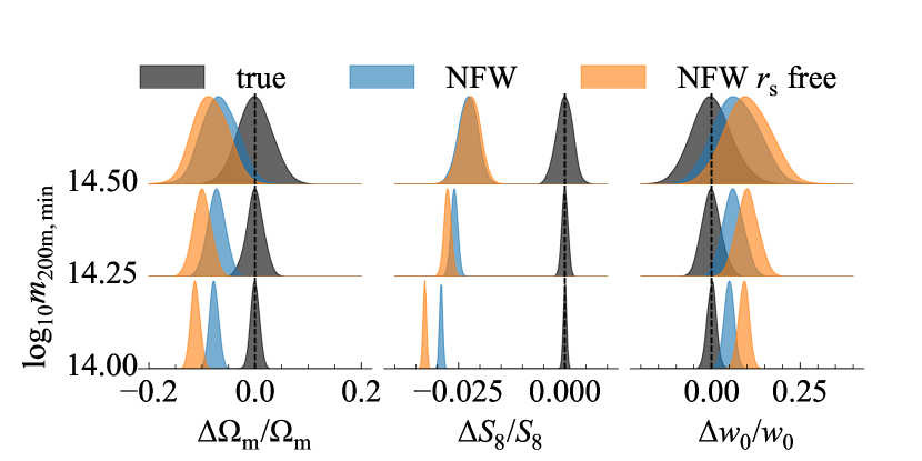
Figure 10: The marginalized maximum a-posteriori probability density functions for $\Omega_{\mathrm{m}}$, $S_{8}=\sigma_{8}(\Omega_{\mathrm{m}}/0.3)^{0.2}$ and $w_{0}$ for 1000 independent stage IV-like cluster abundance surveys with different mass cuts $m_{\mathrm{200m,min}}$ and perfect mass determinations. Gray PDFs show the results for a halo sample with no mass bias. Blue (orange) PDFs include a mass bias due to baryonic effects resulting from an NFW fit to mock weak lensing observations of the reduced shear, with a fixed (free) scale radius, $r_{\mathrm{s}}$. The bias in $S_{8}$ is reduced by a factor of $\approx 8$ if the mass cut is increased from $m_{\mathrm{200m,min}}=10^{14}\,h^{-1}\,\mathrm{M_{\odot}}$ to $m_{\mathrm{200m,min}}=10^{14.5}\,h^{-1}\,\mathrm{M_{\odot}}$, but is still highly significant, while the bias in $\Omega_{\mathrm{m}}$ and $w_{0}$ is reduced to within $2.5\sigma$.

In reality, there will be extra uncertainties due to the photometric redshift estimation of the clusters and the lensed source galaxies, which will scatter clusters between redshift and mass bins. Moreover, the mass uncertainty is a combination of observational systematic uncertainties that evolve differently with mass and redshift (Köhlinger et al., 2015). We have shown that the precision of the inferred cosmological parameters will ultimately be set by the accuracy with which the mass uncertainty of individual cluster masses can be determined. The accuracy of the inferred cosmological parameters will depend on how accurately the bias between the inferred halo masses and the equivalent DMO halo masses can be determined.

Our results clearly indicate the need for more advanced mass inference methods from weak lensing observations and a better calibration between the observed and theoretical halo masses. Under our assumption that the dark matter distribution is not significantly affected by the presence of baryons, it is possible to obtain unbiased halo mass estimates. This suggests that combining measurements of the total and baryonic halo mass, through, e.g., combined weak lensing and X-ray or SZ observations, respectively, would provide significantly less biased mass estimates of the dark matter mass and hence, after scaling by the universal baryon fraction, of the equivalent DMO halo. In Section 5, we explore the possibility of using aperture masses, which are less sensitive to the assumed halo density profile.

5 Aperture masses

In Section 3, we found that we cannot infer unbiased equivalent DMO halo masses from mock weak lensing observations, even when the inferred total halo mass is unbiased. This follows from the deviation of the baryonic component from the assumed NFW density profile and the fact that the baryon fraction is smaller than the universal value in the radial range of the weak lensing observations.

It might be necessary to rethink how we link observed haloes to the theoretical halo mass function, since this is the main baryonic uncertainty. Preferably, the inferred halo masses should differ as little as possible from their equivalent DMO haloes. It has been shown by Herbonnet et al. (2020) that projected halo masses derived from a weak lensing analysis capture the true projected halo mass more accurately than deprojected methods can. The aperture mass is a powerful tool, because it can be computed directly from the data under minimal assumptions about the halo density profile (see e.g. Clowe et al., 1998; Hoekstra et al., 2015). Moreover, we would expect the mass enclosed in a sufficiently large aperture to converge to the equivalent DMO halo mass as long as a larger fraction of the cosmic baryons is included for a larger aperture.

We have performed aperture mass measurements of our mock weak lensing data in the following way. First, we convert the reduced shear to the tangential shear, assuming the best-fitting NFW density profile with a fixed or free scale radius, to compute $\kappa_{\mathrm{NFW}}(R)$

$$\gamma_{\mathrm{T}}(R)=(1-\kappa_{\mathrm{NFW}}(R))g_{\mathrm{T}}(R)\,.$$ (24)

Here, the difference between $\kappa_{\mathrm{NFW}}(R)$ and the true convergence is $\lesssim 2\,\mathrm{per\,cent}$ over the radial range of the observations, resulting in negligible error due to the wrong density profile assumption. Then, we compute the aperture mass using the statistic introduced by Clowe et al. (1998)

$$\zeta_{\mathrm{c}}(R_{1}) =\bar{\kappa}(R{<}R_{1})-\bar{\kappa}(R_{2}<R\leq R_{\mathrm{max}})$$

$$=2\int\limits_{R_{1}}^{R_{2}}\langle\gamma_{\mathrm{T}}\rangle\mathrm{d}\ln R+\frac{2}{1-R_{2}^{2}/R_{\mathrm{max}}^{2}}\int\limits_{R_{2}}^{R_{\mathrm{max}}}\langle\gamma_{\mathrm{T}}\rangle\mathrm{d}\ln R\,,$$ (25)

where $\langle\gamma_{\mathrm{T}}\rangle$ is the azimuthally averaged tangential shear, for which we use the tangential shear from Eq. (24), derived from mock weak lensing observations of the reduced shear. The aperture mass is then given by

$$M(R{<}R_{1})=\pi R^{2}\Sigma_{\mathrm{crit}}(\zeta_{\mathrm{c}}(R_{1})+\bar{\kappa}(R_{2}<R\leq R_{\mathrm{max}}))\,,$$ (26)

where we can use the best-fitting NFW profile to determine $\bar{\kappa}(R_{2}<R\leq R_{\mathrm{max}})$, which is a small correction that again differs negligibly from the true convergence profile due to the NFW assumption. The aperture masses inferred from the above equations recover the true projected halo mass at sub-$\mathrm{per\,cent}$ accuracy over the entire mass range, as we show in the top panel of Fig. 11. Aperture masses are thus a very accurate measure of the true enclosed halo mass, more so due to the fact that they depend so little on assumptions about the underlying true density profile.

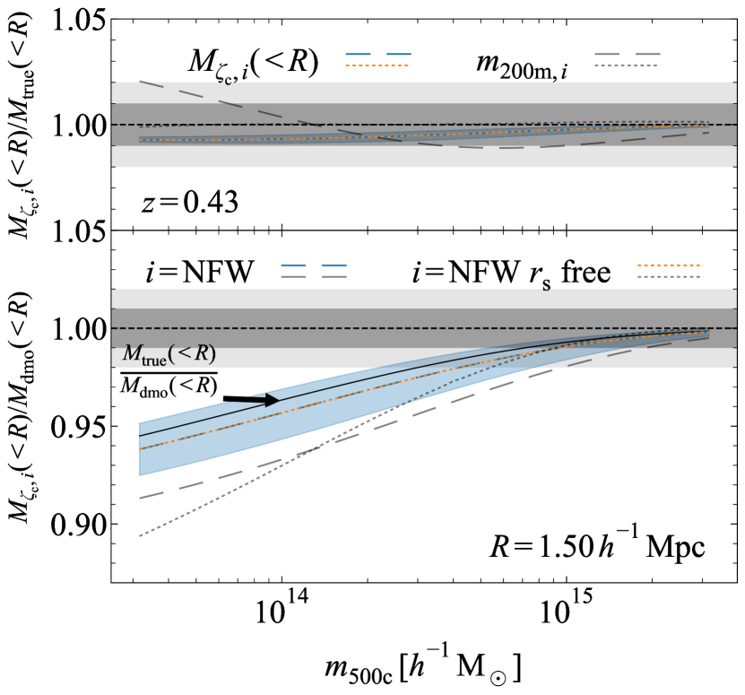
Figure 11: Top panel: The ratio of the total aperture mass within $R<1.5\,h^{-1}\,\mathrm{Mpc}$ derived from mock weak lensing observations, to the true aperture mass. The coloured, dashed and dotted lines show the ratio of the aperture masses inferred for the best-fitting NFW density profiles, with fixed and free scale radius, respectively, to the true aperture mass using the statistic from Eq. (26). The gray dashed and dotted lines show the ratio of the measured and true deprojected masses, $m_{\mathrm{200m,NFW}}/m_{\mathrm{200m,true}}$, for the same NFW fits. For the aperture masses, there is practically no difference between using a fixed or free NFW scale radius, indicating insensitivity to the assumed density profile. The derived aperture mass is within $1\,\mathrm{per\,cent}$ of the true aperture mass for all halo masses. Bottom panel: The ratio of the total aperture mass within $R<1.5\,h^{-1}\,\mathrm{Mpc}$ derived from mock weak lensing observations, to the same aperture mass of the equivalent DMO halo. Line styles are the same as in the top panel. The ratio of the true to the equivalent DMO halo aperture mass is shown as the solid, black line. The aperture masses are less biased with respect to the equivalent DMO mass than the deprojected masses, $m_{\mathrm{200m}}$, which are shown as the gray lines.

However, the problem of linking the observed haloes to their equivalent DMO counterparts still remains, although it is slightly alleviated. In the bottom panel of Fig. 11, we show the ratio of the aperture masses from mock weak lensing observations within a fixed aperture of $R<1.5\,h^{-1}\,\mathrm{Mpc}$ to the mass of the equivalent DMO halo within the same aperture. We choose this aperture size since it is within the range of our mock weak lensing observations in Section 3 and it is larger than the fixed overdensity radius $r_{\mathrm{200m}}$ for haloes with $m_{\mathrm{500c}}<10^{14.5}\,h^{-1}\,\mathrm{M_{\odot}}$, for which $r_{\mathrm{200m}}(z=0.43)\approx 1.3\,h^{-1}\,\mathrm{Mpc}$, resulting in a larger fraction of the universal baryons within it for these abundant haloes. We choose the outer annulus for the correction factor in Eq. (25) between $R_{2}=2.4\,h^{-1}\,\mathrm{Mpc}$ and $R_{\mathrm{max}}=2.5\,h^{-1}\,\mathrm{Mpc}$ such that the NFW correction term is small compared to $\zeta_{\mathrm{c}}$. Aperture masses perform better at recovering the mass of the linked DMO halo than the deprojected NFW masses in Sec. 3 as long as $R_{1}\gtrsim r_{\mathrm{200m}}$, i.e. for all haloes with $m_{\mathrm{500c}}\lesssim 4\times 10^{14}\,h^{-1}\,\mathrm{M_{\odot}}$ at $z=0.43$, as can be seen from the comparison of the coloured dashed and dotted lines with the gray lines in the bottom panel of Fig. 11. This follows from the fact that the halo baryon fractions converge to the cosmic value in the cluster outskirts. This is one of our main conclusions: to link observed haloes to their DMO equivalents, we need to make sure that we are accounting for the ejected baryons. Otherwise, any mass estimate, while not necessarily biased with respect to the true halo mass, will be biased with respect to the equivalent DMO halo mass. It is this latter bias that is fatal for accurate cluster cosmology.

The fact that the statistic in Eq. (26) is practically unbiased with respect to the true aperture mass, regardless of the assumed density profile, makes it an appealing alternative to the deprojected mass determination methods. The problem of calibrating the observed halo masses to their equivalent DMO counterparts, while alleviated, still remains. Since there are so far no theoretical calibrations for the halo aperture mass function, we do not check the performance of the aperture mass determinations for cluster cosmology.

6 Discussion

We have introduced a phenomenological model that reproduces the baryon content inferred from the X-ray surface brightness profiles of the average observed cluster population in the REXCESS survey. We have shown how we can include observed baryonic density profiles in a halo model, while ensuring that the halo baryon fraction converges to the cosmic value in the halo outskirts, by fitting the inferred radial halo baryon fraction with the correct asymptotic value. By assuming that baryons do not significantly alter the distribution of the dark matter, we were able to link observed haloes to their equivalent haloes in a DMO universe, which allowed us to predict their number density. Then, we performed mock weak lensing observations to quantify the effect of the changing halo density profile due to the ejection of baryons on the inferred halo masses. Finally, we investigated the bias due to baryons in the measured cosmological parameters from a number count analysis of a mock cluster sample with masses inferred from weak lensing observations. We have justified that our simplifications result in robust lower bounds on the amplitude of the shift due to baryons of both cluster masses and cosmological parameters from an idealized cluster count cosmology analysis. The survey-specific systematic uncertainties set the statistical significance of these shifts. We have shown that the baryonic bias in the cosmological parameters is highly significant even when not including prior knowledge of the uncertainty in the cluster mass inferred from an observable mass proxy. Now we situate our results in the wider context of the literature.

Balaguera-Antolínez & Porciani (2013) studied the effect of baryons on the cosmological parameters inferred from cluster counts. They used the observed baryon fractions of clusters to infer their equivalent DMO halo masses, similarly to our method. They also find significant biases in the inferred cosmological parameters, mainly a strong suppression in $\Omega_{\mathrm{m}}$ and a slight increase in $\sigma_{8}$ (the exact bias in $\sigma_{8}$ depends on their chosen cluster baryon fraction relation). The amplitude and direction of the bias differ from ours as Balaguera-Antolínez & Porciani (2013) use a single, smaller mock cluster sample ($\approx 2.8\times 10^{4}$ clusters compared to $\approx 1.7\times 10^{5}$) that spans a lower redshift range and they did not include the effect of baryons on the cluster weak lensing mass determinations.

Previously, weak lensing mass determinations have been studied in both DMO (e.g. Bahé et al., 2012) and hydrodynamical simulations (e.g. Henson et al., 2017; Lee et al., 2018). While Bahé et al. (2012) and Henson et al. (2017) find different values for the mass bias, i.e. $\approx 5\,\mathrm{per\,cent}$ and $\approx 10\,\mathrm{per\,cent}$, respectively, they both conclude that these biases result from fitting complex, asymmetric clusters with idealized NFW profiles. (Importantly, these analyses leave the concentration free, which is not the case in most observational analyses.) If this is the case, then we could reduce the weak lensing mass bias by performing a stacked analysis, if we have an unbiased cluster sample. Or, since Henson et al. (2017) find a similar bias at fixed halo mass for haloes in both hydrodynamical and DMO simulations (see the top panel of their fig. 11), it seems feasible to model the mass bias due to triaxiality, substructures and departures from the NFW shape, by performing mock observations of DMO haloes (as in e.g. Dietrich et al., 2019). However, we have shown, as has also been pointed out by Lee et al. (2018), that the distribution of observed cluster baryons implies an intrinsic difference in the density profiles between observed clusters and their DMO equivalents that cannot be captured when assuming a fixed concentration–mass relation. Hence, the inferred halo masses would still be biased, even when accounting for the bias due to halo asymmetry. We found that leaving the concentration of the haloes free mitigates this baryonic mass bias, as was also shown in Lee et al. (2018). However, we showed that the bias in the measured cosmological parameters from a cluster count analysis actually increases when leaving the concentration–mass relation free in the weak lensing analysis. This is because low-mass cluster masses are overestimated when fixing the concentration–mass relation, which compensates for some of the missing baryons and thus reduces the bias with respect to the equivalent DMO halo mass for these abundant clusters.

For cluster cosmology, the vital part is then linking these inferred cluster masses to the equivalent DMO haloes whose number counts we can predict, as argued by Cui et al. (2014), Cusworth et al. (2014) and Velliscig et al. (2014). In the cosmo-OWLS simulations, Velliscig et al. (2014) found differences of $\lesssim 1\,\mathrm{per\,cent}$ between cluster masses in the hydrodynamical and DMO simulations for clusters with $m_{\mathrm{500c}}\gtrsim 10^{14.5}\,h^{-1}\,\mathrm{M_{\odot}}$. In our model, we only find such small biases for haloes with masses $m_{\mathrm{500c}}\gtrsim 10^{15}\,h^{-1}\,\mathrm{M_{\odot}}$. As discussed previously, if we optimistically assume that the predictions from cosmo-OWLS are correct, then this difference could be due to our neglect of the back-reaction of the baryons on the dark matter, and the stellar component. However, for low-mass haloes ($m_{\mathrm{500c}}\lesssim 10^{14.5}\,h^{-1}\,\mathrm{M_{\odot}}$), which will dominate the signal for stage IV-like surveys, these effects are negligible compared to the mass suppression due to the missing baryons.

Using the Magneticum simulation set, Bocquet et al. (2016) and Castro et al. (2020) studied the change in the halo mass function due to baryons and its impact on cluster cosmology. Bocquet et al. (2016) performed a cluster count analysis using halo mass functions calibrated on DMO simulations, to measure the cosmological parameters from a cluster sample generated from the halo mass function of their hydrodynamical simulation. They did not find significant biases for stage III-like surveys, but their shifts in $\Omega_{\mathrm{m}}$ and $S_{8}$ for an eROSITA-like survey are qualitatively similar to our stage IV-like survey predictions. The difference for the stage III-like surveys could be caused by a smaller mismatch between the halo masses in their hydrodynamical and DMO simulations than we infer from observations.

Castro et al. (2020) made Fisher forecasts for a joint cluster number count and clustering analysis of a Euclid-like survey using the baryonic and DMO halo mass functions in the Magneticum simulations. They confirmed that correcting for the baryonic mass bias brings the different halo mass functions into closer agreement. However, they find less significant baryonic mass suppression than we do. The resulting biases in the cosmological parameters are significantly smaller than what we find. This difference is most likely caused by both the lower baryonic mass suppression in Magneticum and a different sample selection. We have chosen a minimum redshift $z_{\mathrm{min}}=0.1$ and a constant limiting mass cut of $m_{\mathrm{200m,min}}=10^{14}\,h^{-1}\,\mathrm{M_{\odot}}$, whereas Castro et al. (2020) use $z_{\mathrm{min}}=0.2$ and a redshift-dependent mass threshold varying around $m_{\mathrm{200c,min}}\approx 10^{14}\,h^{-1}\,\mathrm{M_{\odot}}$ within $0.1\,\mathrm{dex}$ (see their fig. 13). Consequently, our sample includes more low-mass clusters which increases the statistical significance of the bias (as we show in Fig. 10).

An important difference between our work and previous work is that we have used a phenomenological model that reproduces the observed baryon content of clusters. Hence, we do not suffer from the uncertainty related to the assumed subgrid models in hydrodynamical simulations. We only rely on the fact that hydrodynamical simulations imply that the baryonic mass suppression of matched haloes explains the difference between their halo mass function and that derived from DMO simulations. All in all, even though the exact value of the baryonic mass bias between observed and equivalent DMO halo masses, and, consequently, the halo mass function, can differ by up to a few $\mathrm{per\,cent}$ depending on which simulations or observations are used, the general behaviour is the same and implies the need to account for baryonic effects in cluster count cosmology.

7 Conclusions

We set out to investigate the implications for cluster count cosmology of the disconnect between the robust theoretical understanding of cluster-sized ($m_{\mathrm{500c}}>10^{14}\,h^{-1}\,\mathrm{M_{\odot}}$) dark matter-only haloes and the observed cluster population, an issue which was pointed out by Cui et al. (2014), Cusworth et al. (2014), and Velliscig et al. (2014). They found that in hydrodynamical simulations, there is a significant mismatch between the enclosed halo masses at fixed radius that is determined by the halo baryon fraction. We study how the change in the halo density profiles due to the observed distribution of baryons affects the estimated masses from mock weak lensing observations and the resulting cosmological parameters from a cluster number count analysis.

Our model relies on X-ray observations from the REXCESS data (Croston et al., 2008) to constrain the baryonic density profile of cluster-mass haloes. Under the assumption that the dark matter density profile does not change significantly in the presence of baryons, we can link observed haloes to their DMO equivalents. The distribution of a fraction of the DMO halo mass, i.e. the cosmic baryon fraction, will change in the observed halo. Once this link has been established, we can study the change resulting from this baryonic mass bias in cosmological parameters inferred from a number count analysis. We showed that the currently standard weak lensing mass calibrations that assume NFW density profiles and a fixed concentration–mass relation from DMO simulations, are inherently biased for cluster-mass haloes. Fixing the concentration of the halo results in underestimated halo masses since baryons are ejected beyond the typical radial range that the weak lensing observations are sensitive to. The density profile is fit out to radii where baryons are missing and is not flexible enough to capture the increase in baryonic mass towards larger radii. However, we showed that there is enough freedom in the NFW density profile to provide unbiased halo mass estimates if the concentration is left free (see Fig. 5), in agreement with Lee et al. (2018).

However, even unbiased total halo masses result in biased cosmological parameter estimates because of the mismatch between the observed haloes and their DMO equivalents due to ejected baryons (see the middle panel of Fig. 6). This is the dominant baryonic bias. A fiducial weak lensing analysis with fixed concentration–mass relation for a stage IV-like survey would result in highly significantly biased estimates of the cosmological parameters, underestimating $\Omega_{\mathrm{m}}$ and $S_{8}$ by up to $9\,\sigma$ and $76\,\sigma$, respectively, and overestimating $w_{0}$ by $3.5\,\sigma$ (see Fig. 8 and Table 2 for the exact values of the bias). Although leaving the concentration–mass relation free in the weak lensing analysis decreases the bias in the total mass, it actually increases the bias in the cosmological parameters to $13\,\sigma$, $82\,\sigma$ and $6\,\sigma$, respectively. This is because the masses of low-mass clusters are overestimated when fixing the concentration–mass relation, which results in a smaller bias compared to the equivalent DMO mass.

We showed that including a constant uncertainty of $\pm 20\,\mathrm{per\,cent}$ in the individual, unbiased cluster masses only reduces the precision of the inferred cosmological parameters if the mass uncertainty itself is not accurately determined. An uninformative prior on the mass uncertainty decreases the precision of $\Omega_{\mathrm{m}}$, $S_{8}$, and $w_{0}$ by factors of 1.05, 7.8, and 1.02, respectively. However, assuming the mass uncertainty of individual clusters is known to within $\pm 2\,\mathrm{per\,cent}$ results in constraints that are nearly identical to those derived from ideal cluster masses (see Fig. 9 and Table 2).

The picture changes slightly for cluster samples that include the baryonic mass bias. To quantify how neglecting the baryonic mass bias affects the inferred cosmological parameters, we do not account for the mass-dependent baryonic bias when fitting the cluster number counts. Since the model without prior knowledge of the mass uncertainty can vary the mass uncertainty as well as the cosmological parameters, the best-fitting parameters differ between the cases with and without prior knowledge of the mass uncertainty. The uninformative prior on the mass uncertainty decreases the precision of $\Omega_{\mathrm{m}}$, $S_{8}$, and $w_{0}$ by factors of up to 1.1, 10.7, and 1.02, respectively. Knowing the mass uncertainty to within $\pm 2\,\mathrm{per\,cent}$ again results in constraints that cannot be distinguished from those derived from ideal cluster masses (see Fig. 9 and Table 2). The baryonic bias is thus highly statistically significant, even in the presence of mass estimation uncertainties. The accuracy of the cosmological parameters inferred from cluster number counts depends on how accurately inferred halo masses can be linked to their equivalent DMO halo masses. The precision of the cosmological parameter estimates is determined by how accurately the individual cluster mass estimation uncertainty is known.

For stage III-like surveys and assuming a fixed (free) concentration–mass relation, we found biases of $\approx 0.6\,\sigma$ ($0.9\,\sigma$), $3\,\sigma$ ($3\,\sigma$) and $0.1\,\sigma$ ($0.5\,\sigma$) in $\Omega_{\mathrm{m}}$, $S_{8}$, and $w_{0}$, respectively, again, assuming ideal cluster mass estimations (see Fig. 7 and Table 1). However, we stressed that the uncertainties induced by the mass estimation for current stage III-like surveys exceed the statistical uncertainty of our idealized survey.

We also measured aperture masses, since they are expected to provide less biased estimates of the total projected mass than deprojected mass estimates, independently of the assumed density profile of the cluster (see the top panel of Fig. 11) and they are more closely related to the actual weak lensing observable (e.g. Clowe et al., 1998; Herbonnet et al., 2020). However, even though it is slightly alleviated, the problem of linking observed haloes to their DMO equivalents remains (see the middle panel of Fig. 11). We expect the total projected mass to approach the projected DMO mass at large radii (van Daalen et al., 2014). One problem is that correlated large-scale structure becomes important near the cluster virial radius (e.g. Oguri & Hamana, 2011), which requires accurate modelling of the cluster-mass halo bias. We did not include this effect in our model. Using aperture mass estimates would also require a recalibration of halo mass function predictions to this observable.

Any attempt to use clusters for cosmology will need to include a robust method for linking observed haloes to their DMO equivalents. A joint approach, combining weak lensing observations with, for example, hot gas density profiles from from X-ray telescopes like eROSITA—and, in the future, Athena—and/or SZ observations would allow the reconstruction of the cluster dark matter mass, which has already been shown to be much less biased with respect to the equivalent DMO halo mass (Velliscig et al., 2014). This is an essential avenue to be explored. If we cannot robustly establish the link to DMO haloes, we cannot obtain unbiased cosmological parameters.

Data availability

The 1000 mock cluster samples for the stage III-like cluster survey and the MAPs for both the stage III and stage IV-like surveys are publically available through Zenodo at 10.5281/zenodo.4469436. The stage IV-like mock cluster samples can be obtained upon request since they exceed the file size limit of Zenodo. The code for the analysis is available at https://github.com/StijnDebackere/lensing_haloes/.

Appendix A Model fits

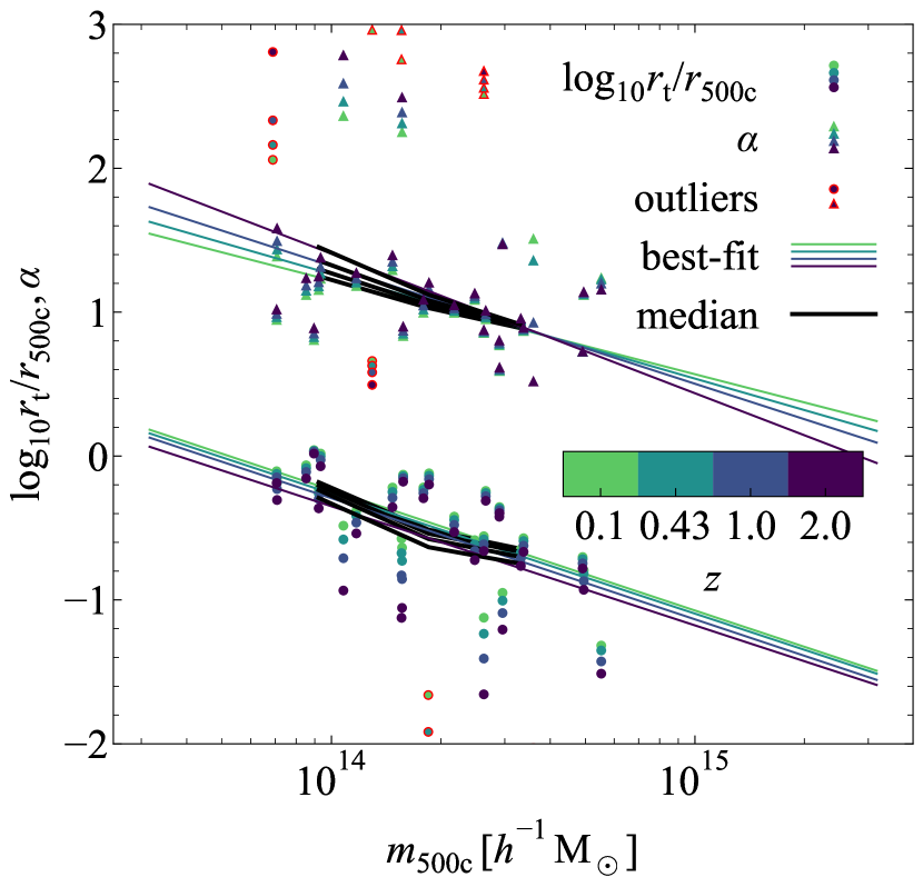
Figure 12: The best-fitting $\log_{10}(r_{\mathrm{t}}/r_{\mathrm{500c}})$ and $\alpha$ values for the REXCESS clusters, self-similarly rescaled to different redshifts (coloured points), their median, mass-binned values (black lines) and the best-fitting linear relations from Eqs. (9) & (10) (coloured lines). The median relation is captured well with the linear model for each redshift. There are some outliers (red outlined markers), whose density profiles are shown in Fig. 13.

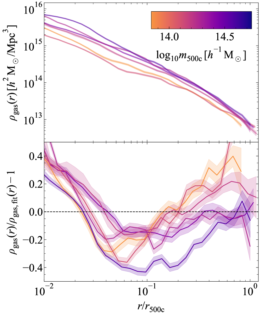
Figure 13: Top panel: The density profiles of the clusters that are outliers to our best-fitting relations for $\log_{10}(r_{\mathrm{t}}/r_{\mathrm{500c}})$ and $\alpha$. Bottom panel: The ratio between the observed hot gas density profiles and our best-fitting model. The outliers cannot be accurately described by our simple monotonic increase in the baryon fraction because they have a high density core.

Fig. 12 shows the best-fitting $r_{\mathrm{t}}(m_{\mathrm{500c}},z)$ and $\alpha(m_{\mathrm{500c}},z)$ for the radial baryon fraction fits (Eq. 7) to each cluster in the REXCESS data, self-similarly scaled to the indicated redshifts. We also show the results for the binned clusters as the black lines, and the best-fitting linear relations, following Eqs. (9) & (10), as the coloured lines. Most of the clusters are described quite well by the best-fitting relations. In Fig. 13, we show the outliers (marked in red in Fig. 12) with $|\Delta\log_{\mathrm{10}}(r_{\mathrm{t}}/r_{\mathrm{500c}})/\log_{\mathrm{10}}(r_{\mathrm{t}}/r_{\mathrm{500c}})|>1.5$ and $|\Delta\alpha/\alpha|>1.5$. All these clusters have a high central density core that cannot be captured by our monotonic relation for the baryon fraction (Eq. 7). These clusters would be better described by, for example, a double beta profile fit. However, these are only 6 out of the total of 31 clusters, spanning the entire mass range. Hence, they do not bias the median mass-binned cluster profiles.

Appendix B Mixed likelihood

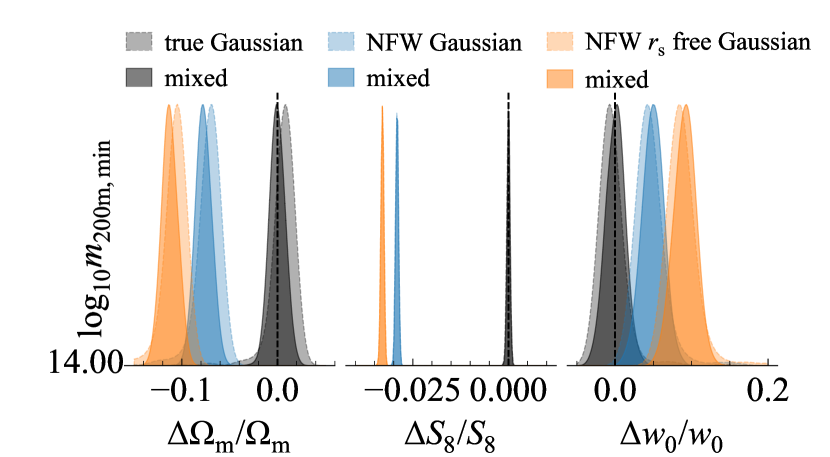
Figure 14: The marginalized maximum a-posteriori probability density functions for $\Omega_{\mathrm{m}}$, $S_{8}=\sigma_{8}(\Omega_{\mathrm{m}}/0.3)^{0.2}$ and $w_{0}$ for 1000 independent stage IV-like cluster abundance surveys assuming a Gaussian likelihood (lightly shaded contours), or a mixed Gaussian-Poisson likelihood (darkly shaded contours). Gray PDFs show the results for a halo sample with no mass bias. Blue (orange) PDFs include a mass bias due to an NFW fit with a fixed (free) scale radius, $r_{\mathrm{s}}$. The Gaussian likelihood biases $\Omega_{\mathrm{m}}$ ($w_{0}$) towards higher (lower) values.

In Fig. 14 we show the difference in cosmological parameter constraints for a stage IV-like cluster abundance survey when using a pure Gaussian likelihood, i.e. Eq. (20), versus the mixed Gaussian-Poisson likelihood that uses Eq. (21) for bins with $N_{\mathrm{obs}}(m_{i},z_{j})<10$. The Gaussian likelihood cannot deal with the discreteness of the number counts at high redshift and high halo masses. The absence of clusters in these bins pushes the theoretical prediction of the halo mass function towards lower values in the Gaussian likelihood. Meanwhile, the number counts for low-mass haloes, which are more abundant and thus better described by the Gaussian likelihood, need to remain the same. For the mass cut $m_{\mathrm{200m,min}}=10^{14}\,h^{-1}\,\mathrm{M_{\odot}}$, the lower number counts for high-mass haloes are achieved by decreasing $w_{0}$ and increasing $\Omega_{\mathrm{m}}$ in such a way that the decrease in number counts for low-mass haloes due to $w_{0}$ is offset by the increase due to $\Omega_{\mathrm{m}}$. $S_{8}$ seems unaffected by the choice in likelihood. The mixed Gaussian-Poisson likelihood results in unbiased cosmological parameter estimates.

References

- Allen et al. (2011) Allen S. W., Evrard A. E., Mantz A. B., 2011, Annu. Rev. Astron. Astrophys., 49, 409
- Applegate et al. (2014) Applegate D. E., et al., 2014, Mon. Not. R. Astron. Soc., 439, 48
- Bahcall et al. (1997) Bahcall N. A., Fan X., Cen R., 1997, Astrophys. J., 485, L53
- Bahé et al. (2012) Bahé Y. M., Mccarthy I. G., King L. J., 2012, Mon. Not. R. Astron. Soc., 421, 1073