Hybrid Trilinear and Bilinear Programming for Aligning Partially Overlapping Point Sets

Abstract

In many applications, we need algorithms which can align partially overlapping point sets and are invariant to the corresponding transformations. In this work, a method possessing such properties is realized by minimizing the objective of the robust point matching (RPM) algorithm. We first show that the RPM objective is a cubic polynomial. We then utilize the convex envelopes of trilinear and bilinear monomials to derive its lower bound function. The resulting lower bound problem has the merit that it can be efficiently solved via linear assignment and low dimensional convex quadratic programming. We next develop a branch-and-bound (BnB) algorithm which only branches over the transformation variables and runs efficiently. Experimental results demonstrated better robustness of the proposed method against non-rigid deformation, positional noise and outliers in case that outliers are not mixed with inliers when compared with the state-of-the-art approaches. They also showed that it has competitive efficiency and scales well with problem size.

$$\begin{CD}E(\mathbf{P},\boldsymbol{\theta})\triangleq\sum_{i,j}p_{ij}\|\mathbf{y}_{j}-\mathbf{T}(\mathbf{x}_{i}|\boldsymbol{\theta})\|^{2}={\color[rgb]{1,0,0}\boxed{\text{trilinear term of }\boldsymbol{\theta}\text{ and }\mathbf{P}}}+{\color[rgb]{0,0,1}\boxed{\text{bilinear term of }\boldsymbol{\theta}\text{ and }\mathbf{P}}}+\text{quadratic term of }\boldsymbol{\theta}+\text{linear term of }\mathbf{P}\\ @V{\text{trilinear}}V{\text{relaxation}}V@V{\text{bilinear}}V{\text{relaxation}}V\\ E_{l}(\mathbf{P},\boldsymbol{\theta})={\color[rgb]{1,0,0}\boxed{\text{linear term of }\boldsymbol{\theta}\text{ and }\mathbf{P}}}+{\color[rgb]{0,0,1}\boxed{\text{linear term of }\boldsymbol{\theta}\text{ and }\mathbf{P}}}+\text{quadratic term of }\boldsymbol{\theta}+\text{linear term of }\mathbf{P}\end{CD}$$

Figure 1: Derivation of a lower bound function of the RPM objective via blinear and trilinear relaxation. Here $\mathbf{x}_{i}$ and $\mathbf{y}_{j}$ denote model point $i$ and scene point $j$, respectively. $\mathbf{P}=\{p_{ij}\}$ denotes the correspondence matrix with $p_{ij}=1$ indicating that there is a correspondence between $\mathbf{x}_{i}$ and $\mathbf{y}_{j}$ and $p_{ij}=0$ otherwise, $\mathbf{T}(\cdot|\boldsymbol{\theta})$ denotes the transformation with parameters $\boldsymbol{\theta}$.

1 Introduction

Registration of 2D/3D point sets is a crucial step in many applications of computer vision, robotics and remote sensing. Apart from difficulties such as non-rigid deformation and positional noise, this problem is particularly challenging when two point sets only partially overlap and are not initially coarsely aligned.

Point set registration can be accomplished by minimizing the objective of the robust point matching (RPM) algorithm [1]. Under the condition that one point set can be embedded in another set, Lian et al. reduced the RPM objective to a concave quadratic function of point correspondence [2]. The resulting function has the important property that the Hessian matrix has a low rank. Thus the branch-and-bound (BnB) algorithm with a low dimensional branching space can be employed for efficient optimization.

This algorithm is generalized to the case when two point sets only partially overlap in [3]. The RPM objective is reduced to a concave function of point correspondence, which, although not quadratic, still has a low rank structure. This enables efficient BnB based optimization. But the branching space of the algorithm is a projected space of point correspondence, whose dimensionality is, different from [2], higher than the number of transformation parameters, leading to slow convergence. Furthermore, to meet the requirement that the objective is concave over the initial simplices, the method enlarges the concavity region of the objective by imposing regularization on transformation where prior information about the transformation is required. However, this causes the method biased in favor of generating solutions only consistent with the prior information.

To address the issue that [3] requires regularization on transformation, Lian and Zhang utilized the constraints of rigid transformations to derive a new objective of point correspondence which is concave over the entire vector space in [4], thus regularization on transformation is not needed when applying the BnB algorithm to the minimization of the objective. From a different perspective, Lian et al. applied the polyhedral annexation (PA) algorithm to the minimization of the objective of RPM [5]. Different from BnB, PA has the advantage of only operating in the concavity region of the objective, thus avoiding the need of regularizing transformation. Nevertheless, like [3], both [4] and [5] still branch a large dimensional projected space of point correspondence, leading to slow convergence. Besides, unlike BnB, PA has the disadvantage of having to cut an increasingly complex polygon as the algorithm progresses. This further worsens the convergence speed of the algorithm.

Aiming at aligning partially overlapping point sets which are not initially coarsely aligned, in this work, we propose an alternative BnB based approach to minimize the objective of RPM. We argue that it is advantageous to retain the transformation variable instead of eliminating them as are the practices of Ref. [2, 3, 4, 5]. The reasons as well as the contributions of this work are listed as follows.

• The objective of RPM is a cubic polynomial. Thus, the convex envelopes of trilinear and bilinear monomials can be utilized to derive the lower bound function, as illustrated in Fig. 1.

• The resulting lower bound problem can be decomposed into separable linear assignment and low dimensional convex quadratic program, both of which can be efficiently solved.

• For the lower bound function to converge to the objective function, we only need to branch over the transformation variable, which is in contrast to previously attempts [3, 4, 5] with large branching spaces. Consequently, the proposed method converges quickly in comparison with previous attempts.

• Unlike [3], our method needs not to impose requirements on transformation. Consequently, the proposed method is invariant to the corresponding transformation and can be applied to situations where initial coarse alignment is not available.

The remainder of the paper is organized as follows: We first review related work (Sec. 2). We then present theoretical framework needed for the development of our lower bound functions (Sec. 3). We next discuss our objective functions and optimization strategies under two different types of transformations (Sec. 4 and 5). We finally present experimental results (Sec. 6) and conclude the paper (Sec. 7).

2 Related work

A survey of point set registration methods can be found in [6]. Here we only mention work close related with ours.

2.1 Local methods

Simultaneous pose and correspondence. The well known ICP method [7] iterates between recovering point correspondence and updating spatial transformation. Despite being efficient, the discrete nature of point correspondence causes the method to be easily trapped in local minima. Zhang et al. improved the robustness of ICP by bounding the rotation angle at each iterative step [8]. Liang supplemented RGB information to the registration process of ICP [9]. The RPM method [1] relaxes point correspondence to be fuzzily valued and uses deterministic annealing (DA) to gradually recover point correspondence. Instead of DA, Sofka et al. use the covariance matrix of the transformation parameters to determine the fuzziness of point correspondence, resulting in better robustness to missing or extraneous structures [10]. Ma et al. used L2E to robustly estimate transformation with application to non-rigid registration [11]. Our method is related with the above methods by also modeling spatial transformation and correspondences. But our objective function is globally minimized. This enables our method to be more robust to disturbances.

Correspondence-free methods. The CPD method [12] casts point matching as the problem of fitting a Guassian mixture model (GMM) representing one point set to another point set. GMMREG [13] uses two GMMs to represent two point sets and minimizes the $L_{2}$-norm distance between them. Support vector parameterized Gaussian mixtures (SVGMs) is used to represent point sets using sparse Gaussian components in [14]. The efficiency of GMM based methods is improved by using filtering to solve the correspondence problem in [15]. The density variation problem of point sets is addressed in [16] by modeling the structure of scene as well. Hierarchical Gaussian mixture representation is used in [17] to improve the speed and accuracy of registration. Ma et al. proposed a Non-Rigid Point Set Registration method by Preserving Global and Local Structures [18].

2.2 Global methods

BnB based methods. The BnB algorithm is a popular global optimization technique. Based on the Lipschitz theory, BnB is used to align 3D shapes in [19]. But the method does not allow outliers or occlusion. BnB is also used to solve for 3D rigid transformation in [20]. But the correspondences need to be known a priori, which limits the applicability of the method. By leveraging the structure of the geometry of 3D rigid motions, Go-ICP [21] globally optimizes the objective of ICP. GOGMA [22] achieves point set registration by aligning the GMMs constructed from the original point sets. Based on stereographic projection, the fast rotation search (FRS) method efficiently recovers 3D rotation between two point sets [23]. A rotation-invariant feature is proposed in [24], resulting in an efficient BnB based registration algorithm. Bayesian nonparametric mixture and a novel approach of tessellating rotation space are proposed in [25], leading to an efficient alignment algorithm. Our BnB based method differs from the above methods in that we also model point correspondences. This enables our method to better handle non-rigid deformation.

Mismatch removal methods. Another line of research focuses on recovering spatial transformation given putative point correspondences. The fast global registration (FGR) method [26] optimizes a robust objective based on duality between line processes and robust estimation. GORE [27] removes large portion of outliers based on geometric operations before RANSAC is invoked. TEASER++ [28] uses a graph-theoretic method to decouple rotation, scale and translation estimation, and adopts a truncated least squares formulation for each subproblem.

2.3 Deep learning methods

Correspondence-free methods. The Lucas–Kanade algorithm is used to align global features of point sets generated by a PointNet [29] network in [30]. This method is improved in [31] by using a decoder to convert the generated global features back into point sets. The fidelity of the global features is guaranteed by minimizing the Chamfer distances between the decoded point sets and the original point sets.

Correspondence-based methods. The FCGF method [32] uses sparse high dimensional convolutions to extract dense feature descriptors from point clouds. This method outperforms many hand-crafted features and PointNet-based methods. It also outperforms a 3D convolution-based method [33]. The deep global registration method [34] uses FCGF feature descriptors for point cloud registration. [35] uncovered several flaws of metric learning based methods. DCP [36] uses DGCNN [37] and Transformer [38] to extract features for each point set and SVD is used to recover rigid transformation. PRNet [39] extends DCP to handle partially overlapping point sets in an iterative way. IDAM [40] considers both geometric and distance features during its point matching process. RIENet [41] calculates feature-to-feature correspondences with neighborhood consensus. [42] performs parital point set registration via matching credibility generation on the global semantic level and geometric feature learning on the local structural level.

3 Convex envelope linearization

In this section, we discuss the convex envelopes of bilinear (Sec. 3.1) and trilinear monomials (Sec. 3.2) and their linearizations. The linearization results play a crutial role in the derivation of the lower bound functions of our objective functions in section 4 and 5.

3.1 Bilinear monomial

The upper part of Eq. 1 shows the convex envelope of a bilinear monomial $xy$. If we directly adopt this form of convex envelope when designing the lower bound function of our objective function, either term in the form of $\max\{(xy)_{l1},(xy)_{l2}\}$ needs to be incorporated into the lower bound function or subproblem in the form of $\min\{\alpha|\alpha\geq(xy)_{l1},\alpha\geq(xy)_{l2}\}$ needs to be incorporated into the lower bound problem. For the former case, the lower bound function is convex but not linear, thus requiring multiple steps of optimization, which is slow and susceptible to numerical inaccuracy issue. For the latter case, the lower bound problem will not take the form of a combinatorial optimization problem, causing the resulting algorithm to be inefficient.

$$\begin{CD}xy@>{\text{ convex envelope}}>{\begin{matrix}\scriptstyle\underline{x}\leq x\leq\overline{x},\\ \scriptstyle\underline{y}\leq y\leq\overline{y}\end{matrix}}>\begin{cases}(xy)_{l1}\triangleq\underline{x}y+x\underline{y}-\underline{x}\underline{y}\leq xy,\\ (xy)_{l2}\triangleq\overline{x}y+x\overline{y}-\overline{x}\overline{y}\leq xy\end{cases}\\ @V{\text{ average}}V{}V\\ (xy)_{l}\triangleq\frac{1}{2}\sum_{i}(xy)_{li}\leq xy\end{CD}$$ (1)

To address the above issues, similar to the practice of [43], we construct a new linear lower bound function $(xy)_{l}$ of $xy$ by averaging the convex envelope inequalities, as illustrated in the lower part of Eq. 1.

Chandraker and Kriegman show that for a bilinear monomial, for its convex envelope to converge to it, we only need to branch over one variable that makes up the bilinear monomial [44]. Similar conclusion can also be drawn about our linear lower bound function. The proof is presented in A.

3.2 Trilinear monomial

The convex envelope of a trilinear monomial $x_{i}x_{j}x_{k}$ depends on the signs of the bounds on variables [45, 46]. Denoting a permutation of $x_{i},x_{j},x_{k}$ by the symbols $x,y,z$, where $\underline{x}\leq x\leq\overline{x}$, $\underline{y}\leq y\leq\overline{y}$ and $\underline{z}\leq z\leq\overline{z}$. For the case $\underline{x}\leq 0,\underline{y}\geq 0,\underline{z}\leq 0,\overline{z}\geq 0$, we can get the convex envelope of $xyz$ as shown in the upper part of Eq. 2.

$$\begin{CD}xyz@>{\begin{matrix}\scriptsize\text{convex}\\ \scriptsize\text{envelope}\end{matrix}}>{\begin{matrix}\scriptstyle\underline{x}\leq x\leq\overline{x},\\ \scriptstyle\underline{y}\leq y\leq\overline{y},\\ \scriptstyle\underline{z}\leq z\leq\overline{z},\\ \scriptstyle\underline{x}\leq 0,\underline{y}\geq 0,\\ \scriptstyle\underline{z}\leq 0,\overline{z}\geq 0\end{matrix}}>\begin{cases}(xyz)_{l1}{\triangleq}\overline{y}\overline{z}x+\overline{x}\overline{z}y+\overline{x}\overline{y}z-2\overline{x}\overline{y}\overline{z}\leq xyz,\\ (xyz)_{l2}\triangleq\overline{y}\underline{z}x+\underline{x}\overline{z}y+\underline{x}\overline{y}z-\underline{x}\overline{y}\underline{z}-\underline{x}\overline{y}\overline{z}\leq xyz,\\ (xyz)_{l3}\triangleq\overline{y}\underline{z}x+\underline{x}\underline{z}y+\underline{x}\underline{y}z-\underline{x}\overline{y}\underline{z}-\underline{x}\underline{y}\underline{z}\leq xyz,\\ (xyz)_{l4}\triangleq\underline{y}\overline{z}x+\overline{x}\underline{z}y+\overline{x}\underline{y}z-\overline{x}\underline{y}\overline{z}-\overline{x}\underline{y}\underline{z}\leq xyz,\\ (xyz)_{l5}\triangleq\underline{y}\underline{z}x+\overline{x}\underline{z}y+\underline{x}\underline{y}z-\overline{x}\underline{y}\underline{z}-\underline{x}\underline{y}\underline{z}\leq xyz,\\ (xyz)_{l6}\triangleq\underline{y}\overline{z}x+\underline{x}\overline{z}y+\phi/(\overline{z}-\underline{z})z-\phi\underline{z}/(\overline{z}-\underline{z})\\ \qquad\qquad-\underline{x}\overline{y}\overline{z}-\overline{x}\underline{y}\overline{z}+\overline{x}\overline{y}\underline{z}\leq xyz\end{cases}\\ @V{\text{ average}}V{}V\\ (xyz)_{l}\triangleq\frac{1}{6}\sum_{i}(xyz)_{li}\leq xyz\end{CD}$$ (2)

Based on the same consideration as stated in Sec. 3.1, we do not directly utilize this form of convex envelope. Instead, we construct a new linear lower bound function $(xyz)_{l}$ of $xyz$ by averaging the convex envelope inequalities, as shown in the lower part of Eq. 2.

For other cases of the bounds on $x,y,z$, we conduct similar operations to linearize the corresponding convex envelopes.

In a similar vein as in Sec. 3.1, for a trilinear monomial, for its linear lower bound function to converge to it, we only need to branch over two variables that make up the trilinear monomial. The proof is presented in A.

4 Case one: spatial transformation is linear with respect to its parameters

In this section, first, we derive our objective function for the case that the spatial transformation is linear with respect to its parameters. Then, we reformulate the objective function due to a requirement when using the convex envelope of a trilinear monomial [46] (Sec. 4.1). Next, we discuss the branching strategy (Sec. 4.2) and use the lower bound functions of bilinear and trilinear terms to derive the lower bound function of our objective function (Sec. 4.3). Finally, we discuss computation of the upper bound (Sec. 4.4) and present the pseudo code of our BnB algorithm (Sec. 4.5).

Suppose there are two point sets $\mathscr{X}=\{\mathbf{x}_{i},1\leq i\leq n_{x}\}$ and $\mathscr{Y}=\{\mathbf{y}_{j},1\leq j\leq n_{y}\}$ in space $\mathbb{R}^{n_{d}}$, where the column vectors $\mathbf{x}_{i}$ and $\mathbf{y}_{j}$ denote coordinates of points $i$ and $j$, repectively. Following [3], we model registration of these two point sets as a mixed linear assignment$-$least square problem:

$$\min E(\mathbf{P},\boldsymbol{\theta})=\sum_{i,j}p_{ij}\|\mathbf{y}_{j}-\mathbf{J}(\mathbf{x}_{i})\boldsymbol{\theta}\|^{2}$$ (3)

$$s.t.\ \mathbf{P}\mathbf{1}_{n_{y}}\leq\mathbf{1}_{n_{x}},\ \mathbf{1}_{n_{x}}^{\top}\mathbf{P}\leq\mathbf{1}_{n_{y}}^{\top},\ \mathbf{1}_{n_{x}}^{\top}\mathbf{P}\mathbf{1}_{n_{y}}=n_{p},\ \mathbf{P}\geq 0,\ \underline{\boldsymbol{\theta}}_{0}\leq\boldsymbol{\theta}\leq\overline{\boldsymbol{\theta}}_{0}$$ (4)

where
$\boldsymbol{\theta}$ : parameters of the spatial transformation $J(\textbf{x}_{i})\boldsymbol{\theta}$. $J(\textbf{x}_{i})$ : the Jacobian matrix of $\mathbf{x}_{i}$. $P$ : correspondence matrix, with element $p_{ij}{=}1$ or $0$ indicating that $\mathbf{x}_{i}$ matches $\mathbf{y}_{j}$ or not. $\mathbf{1}_{n_{x}}^{\top}\mathbf{P}\mathbf{1}_{n_{y}}{=}n_{p}$: the cardinality of matches is required to be equal to a constant integer $n_{p}$. $\underline{\boldsymbol{\theta}}_{0}$ (resp. $\overline{\boldsymbol{\theta}}_{0}$) : the lower (resp. upper) bound of $\boldsymbol{\theta}$.

Based on Eq. [3], $E$ can be written in a concise form as:

$$E(\mathbf{p},\boldsymbol{\theta})=\boldsymbol{\theta}^{\top}\text{mat}(\mathbf{B}\mathbf{p})\boldsymbol{\theta}-2\boldsymbol{\theta}^{\top}\mathbf{A}\mathbf{p}+\boldsymbol{\rho}^{\top}\mathbf{p}$$ (5)

where
$\mathbf{p}\triangleq\text{vec}(\mathbf{P})$: a vector. $\boldsymbol{\rho}\triangleq\mathbf{1}_{n_{x}}\otimes\widetilde{\mathbf{y}}$: a vector. $\mathbf{A}\triangleq(\mathbf{J}^{\top}\otimes\mathbf{y}^{\top})\mathbf{W}^{n_{x},n_{y}}_{n_{d}}$: a matrix. $\mathbf{B}\triangleq(\mathbf{J}_{2}^{\top}\otimes\mathbf{I}_{n_{\theta}})\mathbf{W}^{n_{x},1}_{n_{\theta}}(\mathbf{I}_{n_{x}}\otimes\mathbf{1}_{n_{y}}^{\top})$: a matrix. $\mathbf{J}\triangleq\begin{bmatrix}\mathbf{J}^{\top}(\mathbf{x}_{1}),\dots,\mathbf{J}^{\top}(\mathbf{x}_{n_{x}})\end{bmatrix}^{\top}$: a matrix. $\mathbf{J}_{2}\triangleq\begin{bmatrix}\mathbf{J}(\mathbf{x}_{1})^{\top}\mathbf{J}(\mathbf{x}_{1}),\ldots,\mathbf{J}(\mathbf{x}_{n_{x}})^{\top}\mathbf{J}(\mathbf{x}_{n_{x}})\end{bmatrix}^{\top}$: a matrix. $\mathbf{W}^{m,n}_{d}\triangleq\mathbf{I}_{m}\otimes\begin{bmatrix}\mathbf{I}_{n}\otimes(\mathbf{e}_{d}^{1})^{\top},\dots,\mathbf{I}_{n}\otimes(\mathbf{e}_{d}^{d})^{\top}\end{bmatrix}^{\top}$: a matrix. $\mathbf{y}\triangleq\begin{bmatrix}\mathbf{y}_{1}^{\top},\dots,\mathbf{y}_{n_{y}}^{\top}\end{bmatrix}^{\top}$: a vector. $\widetilde{\mathbf{y}}\triangleq\begin{bmatrix}\|\mathbf{y}_{1}\|_{2}^{2},\dots,\|\mathbf{y}_{n_{y}}\|_{2}^{2}\end{bmatrix}^{\top}$: a vector. $\text{vec}(\cdot)$: vectorization of a matrix by concatenating rows. $n_{\theta}$: the dimensionality of ${\boldsymbol{\theta}}$. $\mathbf{e}_{d}^{i}$: the $d$-dimensional column vector with only one nonzero unit element at the $i$-th position. $\mathbf{1}_{n_{x}}$: the $n_{x}$-dimensional vector of all ones. $\mathbf{I}_{d}$: the $d\times d$ identity matrix. $\otimes$: the Kronecker product. $\text{mat}(\cdot)$: reconstructs a matrix from a vector, which is the inverse of the operator $\text{vec}(\cdot)$.

Since $\mathbf{1}^{\top}_{n_{x}n_{y}}\mathbf{p}=n_{p}$, a constant, for rows of $\mathbf{B}$ containing identical elements, the result of them multiplied by $\mathbf{p}$ can be replaced by constants. Also, redundant rows can be removed. Since $\text{mat}(\mathbf{B}\mathbf{p})$ is a symmetric matrix, $\mathbf{B}$ will contain redundant rows. Based on these analyses, we hereby denote $\mathbf{B}_{2}$ as the matrix formed as a result of $\mathbf{B}$ removing such rows. (Please refer to Sec. 6.1 for examples of $\mathbf{B}_{2}$). Consequently, $E$ can be rewritten as

$$E(\mathbf{p},\boldsymbol{\theta})=\boldsymbol{\theta}^{\top}\left[\text{mat}(\mathbf{K}\mathbf{B}_{2}\mathbf{p}){+}\mathbf{C}\right]\boldsymbol{\theta}{-}2\boldsymbol{\theta}^{\top}\mathbf{A}\mathbf{p}{+}\boldsymbol{\rho}^{\top}\mathbf{p}$$ (6)

where the nonzero elements of the constant matrix $\mathbf{C}$ correspond to the rows of $\mathbf{B}$ containing identical elements. The elements of the constant matrix $\mathbf{K}$ take values in $\{0,1\}$ and record the correspondences between the rows of $\mathbf{B}_{2}$ and those of $\mathbf{B}$.

4.1 Objective function reformulation

The convex envelope of a trilinear monomial presented in [46] only holds under the condition that at least one variable that makes up the monomial has a range containing the origin, whereas for the trilinear term $\boldsymbol{\theta}^{\top}\text{mat}(\mathbf{K}\mathbf{B}_{2}\mathbf{p})\boldsymbol{\theta}$ in our objective function, such a condition can be violated. To address this issue, since our branching strategy (to be presented in Sec. 4.2) is that the range of $\theta_{i}$ changes during the BnB iterations, whereas the range of $[\text{mat}(\mathbf{K}\mathbf{B}_{2}\mathbf{p})]_{ij}$ remains fixed, therefore, we seek to replace $\text{mat}(\mathbf{K}\mathbf{B}_{2}\mathbf{p})$ by a proper matrix such that this condition can be satisfied. The procedure is as follows:

We build a constant symmetric matrix $\mathbf{D}$ such that all the elements of $\text{mat}(\mathbf{K}\mathbf{B}_{2}\mathbf{p})-\mathbf{D}$ have ranges containing the origin. This can be accomplished as follows: We first choose $\mathbf{p}_{0}\in\Omega$, where $\Omega$ represents the feasible region of $\mathbf{p}$, as is defined by (4). (In this paper, $\mathbf{p}_{0}$ is chosen as $\frac{n_{p}}{n_{x}n_{y}}\mathbf{1}_{n_{x}n_{y}}$, corresponding to the case that point correspondence is the fuzziest.) We then let $\mathbf{D}=\text{mat}(\mathbf{K}\mathbf{B}_{2}\mathbf{p}_{0})$. We now have

Proposition 1

All the elements of $\text{mat}(\mathbf{K}\mathbf{B}_{2}\mathbf{p})-\mathbf{D}$ have ranges containing the origin.

Proof: Since $\mathbf{p}_{0}\in\Omega$, we have $\mathbf{D}\in\{\text{mat}(\mathbf{K}\mathbf{B}_{2}\mathbf{p})|\mathbf{p}\in\Omega\}$. Therefore, $0\in\{[\text{mat}(\mathbf{K}\mathbf{B}_{2}\mathbf{p})-\mathbf{D}]_{ij}|\mathbf{p}\in\Omega\}$.

Our experiments indicate that different choices of $\mathbf{p}_{0}$ (and thus $\mathbf{D}$) lead to almost the same alignment results. Based on the above analysis, $E$ is reformulated as:

$$E(\mathbf{p},\boldsymbol{\theta})=\boldsymbol{\theta}^{\top}[\text{mat}(\mathbf{K}\mathbf{B}_{2}\mathbf{p})-\mathbf{D}]\boldsymbol{\theta}+\boldsymbol{\theta}^{\top}(\mathbf{C}+\mathbf{D})\boldsymbol{\theta}-2\boldsymbol{\theta}^{\top}\mathbf{A}\mathbf{p}+\boldsymbol{\rho}^{\top}\mathbf{p}$$ (7)

4.2 Branching strategy

Based on the result in Sec. 3.1, for the bilinear term $-2\boldsymbol{\theta}^{\top}\mathbf{A}\mathbf{p}$, for its linear lower bound function to converge to it, we only need to branch the range of $\boldsymbol{\theta}$ and leave the range of $-2\mathbf{A}\mathbf{p}$ fixed. Here the range of $-2\mathbf{A}\mathbf{p}$ can be computed as

$$\min_{\mathbf{p}\in\Omega}(-2\mathbf{A}\mathbf{p})_{i}\leq(-2\mathbf{A}\mathbf{p})_{i}\leq\max_{\mathbf{p}\in\Omega}(-2\mathbf{A}\mathbf{p})_{i}$$ (8)

In a similar vein, based on the result in Sec. 3.2, for the trilinear term $\boldsymbol{\theta}^{\top}[\text{mat}(\mathbf{K}\mathbf{B}_{2}\mathbf{p})-\mathbf{D}]\boldsymbol{\theta}$, for its linear lower bound function to converge to it, we only need to branch the range of $\boldsymbol{\theta}$ and leave the range of $\text{mat}(\mathbf{K}\mathbf{B}_{2}\mathbf{p})-\mathbf{D}$ fixed since $\boldsymbol{\theta}$ constitutes two sets of variables that make up $\boldsymbol{\theta}^{\top}[\text{mat}(\mathbf{K}\mathbf{B}_{2}\mathbf{p})-\mathbf{D}]\boldsymbol{\theta}$. Here the range of $\text{mat}(\mathbf{K}\mathbf{B}_{2}\mathbf{p})-\mathbf{D}$ can be computed as

$$\min_{\mathbf{p}\in\Omega}[\text{mat}(\mathbf{K}\mathbf{B}_{2}\mathbf{p})-\mathbf{D}]_{ij}{\leq}[\text{mat}(\mathbf{K}\mathbf{B}_{2}\mathbf{p})-\mathbf{D}]_{ij}{\leq}\max_{\mathbf{p}\in\Omega}[\text{mat}(\mathbf{K}\mathbf{B}_{2}\mathbf{p})-\mathbf{D}]_{ij}$$ (9)

In conclusion, in our BnB algorithm, we only need to branch over $\boldsymbol{\theta}$. Therefore, the dimension of the branching space of our BnB algorithm is low and the proposed algorithm can converge quickly.

4.3 Lower bound

Based on the results in Sec. 3, we can obtain the lower bound function $E_{l}$ of $E$ by respectively deriving the lower bound functions of the bilinear and trilinear terms, as illustrated in Eq. 10.

$$\begin{CD}E(\mathbf{p},\boldsymbol{\theta})=\boldsymbol{\theta}^{\top}(\mathbf{C}+\mathbf{D})\boldsymbol{\theta}+\boldsymbol{\rho}^{\top}\mathbf{p}+{\color[rgb]{1,0,0}\boxed{\boldsymbol{\theta}^{\top}[\text{mat}(\mathbf{K}\mathbf{B}_{2}\mathbf{p})-\mathbf{D}]\boldsymbol{\theta}}}+{\color[rgb]{0,0,1}\boxed{-2\boldsymbol{\theta}^{\top}\mathbf{A}\mathbf{p}}}\\ @V{\text{trilinear}}V{\text{relaxation }}V@V{\text{bilinear}}V{\text{relaxation}}V\\ E_{l}(\mathbf{p},\boldsymbol{\theta})=\boldsymbol{\theta}^{\top}(\mathbf{C}+\mathbf{D})\boldsymbol{\theta}+\boldsymbol{\rho}^{\top}\mathbf{p}+{\color[rgb]{1,0,0}\boxed{\begin{matrix}\boldsymbol{\theta}^{\top}\mathbf{H}^{0}\mathbf{1}_{n_{\theta}}+\text{tr}([\text{mat}(\mathbf{K}\mathbf{B}_{2}\mathbf{p})-\mathbf{D}]^{\top}\mathbf{H}^{1})+\mathbf{1}_{n_{\theta}}^{\top}\mathbf{H}^{2}\mathbf{1}_{n_{\theta}}\end{matrix}}}+{\color[rgb]{0,0,1}\boxed{\begin{matrix}\boldsymbol{\theta}^{\top}\mathbf{g}^{0}+(\mathbf{g}^{1})^{\top}(-2\mathbf{A}\mathbf{p})+\mathbf{1}_{n_{\theta}}^{\top}\mathbf{g}^{2}\end{matrix}}}\end{CD}$$ (10)

Consequently $E_{l}$ can be written into the following concise form:

$$\min E_{l}(\mathbf{p},\boldsymbol{\theta})\triangleq\boldsymbol{\theta}^{\top}(\mathbf{C}+\mathbf{D})\boldsymbol{\theta}{+}\mathbf{m}_{0}^{\top}\boldsymbol{\theta}{+}\mathbf{m}_{1}^{\top}\mathbf{p}{+}m_{2}$$ (11)

where $\mathbf{m}_{0}$ and $\mathbf{m}_{1}$ are constant vectors and $m_{2}$ is a constant scalar.

It is obvious that the minimization of $E_{l}$ under the constraints $\underline{\boldsymbol{\theta}}\leq\boldsymbol{\theta}\leq\overline{\boldsymbol{\theta}},\ \mathbf{p}\in\Omega$ can be decomposed into separate optimizations over $\mathbf{p}$ and $\boldsymbol{\theta}$. $\mathbf{p}$ is recovered by solving the following linear assignment problem:

$$\min_{\mathbf{p}\in\Omega}\mathbf{m}_{1}^{\top}\mathbf{p}$$ (12)

$\boldsymbol{\theta}$ is recovered by solving the following low dimensional quadratic optimization problem:

$$\min\ \boldsymbol{\theta}^{\top}(\mathbf{C}+\mathbf{D})\boldsymbol{\theta}+\mathbf{m}_{0}^{\top}\boldsymbol{\theta}$$ (13)

$$s.t.\quad\underline{\boldsymbol{\theta}}\leq\boldsymbol{\theta}\leq\overline{\boldsymbol{\theta}}$$ (14)

Solvers such as the matlab function $quadprog$ can be employed for this problem. The following result indicates that this is a convex problem.

Proposition 2

We have $\mathbf{C}+\mathbf{D}\succeq 0$.

Proof: For any $\mathbf{p}\in\Omega$, we have $\text{mat}(\mathbf{B}\mathbf{p})=\mathbf{J}_{2}^{\top}((\mathbf{P}\mathbf{1}_{n_{y}})\otimes\mathbf{I}_{n_{\theta}})=\sum_{i}\mathbf{J}_{i}^{\top}\mathbf{J}_{i}(\mathbf{P}\mathbf{1}_{n_{y}})_{i}\succeq 0$. Since $\mathbf{p}_{0}\in\Omega$, thus we have $\text{mat}(\mathbf{B}\mathbf{p}_{0})=\text{mat}(\mathbf{K}\mathbf{B}_{2}\mathbf{p}_{0})+\mathbf{C}=\mathbf{D}+\mathbf{C}\succeq 0$.

4.4 Upper bound

By plugging the $\mathbf{p},\boldsymbol{\theta}$ solutions yielded during the computation of the lower bound into $E(\mathbf{p},\boldsymbol{\theta})$, we can get an upper bound. Nevertheless, the $\boldsymbol{\theta}$ solution may deviate significantly from the optimal $\boldsymbol{\theta}$ especially during the early iterations of the BnB algorithm, causing the computed upper bound to be poor. To address this issue, based on a result of [3], the objective function $E(\mathbf{p},\boldsymbol{\theta})$ can be rewritten as a function of $\mathbf{p}$ by eliminating $\boldsymbol{\theta}$ (please also refer to B for detailed derivation):

$$E(\mathbf{p})=-\mathbf{p}^{\top}\mathbf{A}^{\top}[\text{mat}(\mathbf{K}\mathbf{B}_{2}\mathbf{p})+\mathbf{C}]^{-1}\mathbf{A}\mathbf{p}+\boldsymbol{\rho}^{\top}\mathbf{p}$$ (15)

Therefore, we can plug the computed $\mathbf{p}$ into this function to get a value of $E$, which is used as an upper bound.

4.5 Branch-and-Bound

Based on the aforementioned preparations, we are now ready to employ the BnB algorithm to optimize $E$. The algorithm is summarized in Algo. 1, where the initial hypercube $M$ is chosen as the intial range of $\boldsymbol{\theta}$.

Since the optimal $\boldsymbol{\theta}$ solution depends on the relative size and position of two point sets, in this work, we rescale point sets $\mathscr{X}$ and $\mathscr{Y}$ to be unit sized and translate them to be centered at the origin before performing registration. Unless otherwise stated, we set the initial range of $\boldsymbol{\theta}$ as $[-3\mathbf{1}_{n_{\theta}},3\mathbf{1}_{n_{\theta}}]$.

1Initialization

2Set tolerance error $\epsilon>0$ and initial hypercube $M$. Let $\mathscr{M}_{1}=\mathscr{N}_{1}=\{M\}$ where $\mathscr{M}_{k}$ and $\mathscr{N}_{k}$ denote the collection of all hypercubes and the collection of active hypercubes at iteration $k$, respectively.

3for $k=1,2,\ldots$ do

4      

5      For each hypercube $M\in\mathscr{N}_{k}$, minimize the lower bound function $E_{l}$ to obtain the optimal point correspondence solution $\mathbf{p}(M)$ and the optimal value $\beta(M)$. $\beta(M)$ is a lower bound for $M$.

6      Let $\mathbf{p}^{k}$ be the best among all feasible solutions so far encountered: $\mathbf{p}^{k-1}$ and all $\mathbf{p}(M)$ for $M\in\mathscr{N}_{k}$. Delete all $M\in\mathscr{M}_{k}$ such that $\beta(M)\geq E(\mathbf{p}^{k})-\epsilon$. Let $\mathscr{R}_{k}$ be the remaining collection of hypercubes.

7      If $\mathscr{R}_{k}=\emptyset$, terminate: $\mathbf{p}^{k}$ is the global $\epsilon-$minimum solution.

8      Select the hypercube $M$ yielding the lowest lower bound and divide it into two sub-hypercubes $M_{1}$, $M_{2}$ by bisecting the longest edge.

9      Let $\mathscr{N}_{k+1}=\{M_{1},M_{2}\}$ and $\mathscr{M}_{k+1}=(\mathscr{R}_{k}\backslash M)\cup\mathscr{N}_{k+1}$.

10 end for

11

Algorithm 1 A BnB algorithm for minimizing $E$

4.6 Convergence of the BnB algorithm

To evaluate convergence of the proposed BnB algorithm, we use the separate outliers and inliers test described in Sec. 6.1.1 where the outlier to data ratio is chosen as $0.3$. The experimental result is reported in Fig. 2. It shows that: 1) The duality gap decreases quickly initially but slowly later on, and there is noticeable duality gap even after many iterations. 2) Smaller initial range of $\boldsymbol{\theta}$ leads to tighter duality gap (with both better upper and lower bounds). So in practice, if there is more information about the range of $\boldsymbol{\theta}$, this information can be utilized to reduce duality gap of the proposed method. 3) Easier problems (e.g., the fish test versus the character test) also leads to tighter duality gap.

Properties 1) and 3) suggest that employing a fixed duality gap threshold as the stopping criterion for all types of problems may not be a good idea. It may happen that a duality gap threshold is set too small for a hard problem, leading to long running time, yet it is set too large for an easy problem, causing premature early termination. So in this paper, instead of using duality gap threshold as the stopping criterion, we use the maximum branching depth as the stopping criterion. With this choice, our method is no longer an $\epsilon-$globally optimal algorithm. Nevertheless, it differs from traditional heuristic methods in that it can also return a degree (i.e., duality gap) to which the solution is different from the optimal solution.

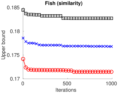
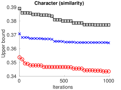
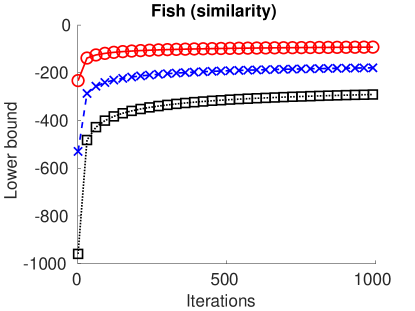
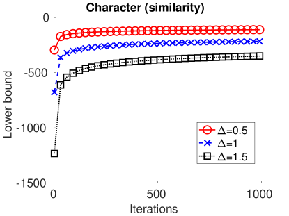
Figure 2: Upper (first row) and lower bounds (second row) generated in each iteration of the proposed algorithm. We test our method with $n_{p}$ value chosen as the ground truth and with different initial ranges $[\boldsymbol{\theta}_{gt}-\Delta,\boldsymbol{\theta}_{gt}+\Delta]$ of $\boldsymbol{\theta}$, where $\boldsymbol{\theta}_{gt}$ denotes the ground truth $\boldsymbol{\theta}$ solution and the margin $\Delta$ is respectively chosen as $0.5$, $1$ and $1.5$.

5 Case two: 3D rigid transformation

In this section, we first discuss the derivation of our objective function for the case that the transformation is 3D rigid. Then, we discuss the branching strategy (Sec. 5.1). Next, we utilize the lower bound functions of bilinear and trilinear terms to derive the lower bound function of the objective (Sec. 5.2). Then, we discuss the computation of upper bound and computation of the range of $\mathbf{R}$ from the range of $\mathbf{r}$ (Sec. 5.3 and 5.4). Next, we use point set normalization to satisfy a requirement when using the convex envelope of a trilinear monomial [46] (Sec. 5.5). Finally, we present the BnB algorithm (Sec. 4.5) and discuss its convergence property (Sec. 5.7).

A 3D affine transformation has many parameters, causing our algorithm to be inefficient. Therefore, for the 3D case, we instead focus on rigid transformation and develop corresponding objective function and optimization strategy.

Using the angle-axis representation, each 3D rotation can be represented as a 3D vector $\mathbf{r}$, with axis $\mathbf{r}/\|\mathbf{r}\|$ and angle $\|\mathbf{r}\|$. The corresponding $3\times 3$ rotation matrix $\mathbf{R}\in\mathbb{SO}_{3}$ for $\mathbf{r}$ can be obtained using matrix exponential map as [21]

$$\mathbf{R}=\mathbf{I}_{3}+\frac{[\mathbf{r}]_{\times}\sin\|\mathbf{r}\|}{\|\mathbf{r}\|}+\frac{[\mathbf{r}]_{\times}^{2}(1-\cos\|\mathbf{r}\|)}{\|\mathbf{r}\|^{2}}$$ (16)

where $[\cdot]_{\times}$ denotes the skew-symmetric matrix representation:

$$[\mathbf{r}]_{\times}=\begin{bmatrix}0&-r_{3}&r_{2}\\ r_{3}&0&-r_{1}\\ -r_{2}&r_{1}&0\end{bmatrix}$$ (17)

where $r_{i}$ is the $i$-th element of $\mathbf{r}$.

Following [4], point set registration is modeled as a linear assignment$-$least square problem:

$$\min E(\mathbf{P},\mathbf{R},\mathbf{t})=\sum p_{ij}\|\mathbf{y}_{j}-\mathbf{R}\mathbf{x}_{i}-\mathbf{t}\|^{2}$$

$$=\mathbf{1}_{n_{x}}^{\top}\mathbf{P}\widetilde{\mathbf{y}}{+}\widetilde{\mathbf{x}}^{\top}\mathbf{P}\mathbf{1}_{n_{y}}{+}n_{p}\|\mathbf{t}\|^{2}{-}2\text{tr}(\mathbf{R}\mathbf{X}^{\top}\mathbf{P}\mathbf{Y}){-}2\mathbf{t}^{\top}(\mathbf{Y}^{\top}\mathbf{P}^{\top}\mathbf{1}_{n_{x}}{-}\mathbf{R}\mathbf{X}^{\top}\mathbf{P}\mathbf{1}_{n_{y}})$$ (18)

$$s.t.\quad\mathbf{P}\in\Omega,\ \mathbf{R}\in\mathbb{SO}_{3},\ \underline{\mathbf{r}}_{0}\leq\mathbf{r}\leq\overline{\mathbf{r}}_{0},\ \underline{\mathbf{t}}_{0}\leq\mathbf{t}\leq\overline{\mathbf{t}}_{0}$$ (19)

where the transformation is chosen as a rigid transformation with rotation matrix $\mathbf{R}$ and translation $\mathbf{t}$. The matrix $\mathbf{X}\triangleq\begin{bmatrix}\mathbf{x}_{1},\ldots,\mathbf{x}_{n_{x}}\end{bmatrix}^{\top}$ and $\mathbf{Y}\triangleq\begin{bmatrix}\mathbf{y}_{1},\ldots,\mathbf{y}_{n_{y}}\end{bmatrix}^{\top}$. The vector $\widetilde{\mathbf{x}}\triangleq\begin{bmatrix}\|\mathbf{x}_{1}\|_{2}^{2},\dots,\|\mathbf{x}_{n_{x}}\|_{2}^{2}\end{bmatrix}^{\top}$. The constant vectors $\underline{\mathbf{r}}_{0}$, $\overline{\mathbf{r}}_{0}$ (resp. $\underline{\mathbf{t}}_{0}$, $\overline{\mathbf{t}}_{0}$) define the lower and upper bounds of $\mathbf{r}$ (resp. $\mathbf{t}$).

5.1 Branching strategy

Based on the result in Sec. 3.1, for the bilinear term $-2\mathbf{t}^{\top}\mathbf{Y}^{\top}\mathbf{P}^{\top}\mathbf{1}$, for its linear lower bound function to converge to it, we only need to branch the range of $\mathbf{t}$ and leave the range of $-2\mathbf{Y}^{\top}\mathbf{P}^{\top}\mathbf{1}$ fixed. Here, the range of $-2\mathbf{Y}^{\top}\mathbf{P}^{\top}\mathbf{1}$ can be computed as

$$\min_{\mathbf{p}\in\Omega}(-2\mathbf{Y}^{\top}\mathbf{P}^{\top}\mathbf{1})_{i}\leq(-2\mathbf{Y}^{\top}\mathbf{P}^{\top}\mathbf{1})_{i}\leq\max_{\mathbf{p}\in\Omega}(-2\mathbf{Y}^{\top}\mathbf{P}^{\top}\mathbf{1})_{i}$$ (20)

Likewise, for the bilinear term $-2\text{tr}(\mathbf{R}\mathbf{X}^{\top}\mathbf{P}\mathbf{Y})$, we only need to branch the range of $\mathbf{r}$ (since the range of $\mathbf{r}$ determines the range of $\mathbf{R}$) and leave the range of $-2\mathbf{X}^{\top}\mathbf{P}\mathbf{Y}$ fixed. Here, the range of $-2\mathbf{X}^{\top}\mathbf{P}\mathbf{Y}$ can be computed as

$$\min_{\mathbf{p}\in\Omega}(-2\mathbf{X}^{\top}\mathbf{P}\mathbf{Y})_{ij}\leq(-2\mathbf{X}^{\top}\mathbf{P}\mathbf{Y})_{ij}\leq\max_{\mathbf{p}\in\Omega}(-2\mathbf{X}^{\top}\mathbf{P}\mathbf{Y})_{ij}$$ (21)

In a similar vein, based on the result in Sec. 3.2, for the trilinear term $2\mathbf{t}^{\top}\mathbf{R}\mathbf{X}^{\top}\mathbf{P}\mathbf{1}$, for its linear lower bound function to converge to it, we only need to branch the ranges of $\mathbf{r}$ and $\mathbf{t}$ and leave the range of $2\mathbf{X}^{\top}\mathbf{P}\mathbf{1}$ fixed. Here, the range of $2\mathbf{X}^{\top}\mathbf{P}\mathbf{1}$ can be computed as

$$\min_{\mathbf{p}\in\Omega}(2\mathbf{X}^{\top}\mathbf{P}\mathbf{1})_{j}\leq(2\mathbf{X}^{\top}\mathbf{P}\mathbf{1})_{j}\leq\max_{\mathbf{p}\in\Omega}(2\mathbf{X}^{\top}\mathbf{P}\mathbf{1})_{j}$$ (22)

In conclusion, in our BnB algorithm, we only need to branch over $\mathbf{r}$ and $\mathbf{t}$. Thus, the dimension of the branching space of our BnB algorithm is low and our algorithm can converge quickly.

5.2 Lower bound

Based on the results in Sec. 3, we can obtain the lower bound function $E_{l}$ of $E$ by respectively deriving the lower bound functions of the bilinear and trilinear terms, as illustrated in Eq. 23.

$$\begin{CD}E(\mathbf{P},\mathbf{R},\mathbf{t}){=}\begin{matrix}\mathbf{1}_{n_{x}}^{\top}\mathbf{P}\widetilde{\mathbf{y}}{+}\widetilde{\mathbf{x}}^{\top}\mathbf{P}\mathbf{1}_{n_{y}}{+}n_{p}\|\mathbf{t}\|^{2}\end{matrix}{\color[rgb]{0,0,1}\boxed{-2\text{tr}(\mathbf{R}\mathbf{X}^{\top}\mathbf{P}\mathbf{Y})}}{\color[rgb]{0,0,1}\boxed{-2\mathbf{t}^{\top}\mathbf{Y}^{\top}\mathbf{P}^{\top}\mathbf{1}_{n_{x}}}}{\color[rgb]{1,0,0}\boxed{+2\mathbf{t}^{\top}\mathbf{R}\mathbf{X}^{\top}\mathbf{P}\mathbf{1}_{n_{y}}}}\\ @V{\text{bilinear}}V{\text{relaxation}}V@V{\text{bilinear}}V{\text{relaxation}}V@V{\text{trilinear}}V{\text{relaxation}}V\\ E_{l}(\mathbf{P},\mathbf{R},\mathbf{t}){=}\begin{matrix}\mathbf{1}_{n_{x}}^{\top}\mathbf{P}\widetilde{\mathbf{y}}{+}\widetilde{\mathbf{x}}^{\top}\mathbf{P}\mathbf{1}_{n_{y}}{+}n_{p}\|\mathbf{t}\|^{2}\end{matrix}{+}{\color[rgb]{0,0,1}\boxed{\begin{matrix}\text{tr}(\mathbf{C}^{0}\mathbf{R}^{\top}){-}2\text{tr}(\mathbf{C}^{1}\mathbf{X}^{\top}\mathbf{P}\mathbf{Y})\\ +\mathbf{1}_{3}^{\top}\mathbf{C}^{2}\mathbf{1}_{3}\end{matrix}}}+{\color[rgb]{0,0,1}\boxed{\begin{matrix}\mathbf{t}^{\top}\mathbf{d}^{0}{-}2\mathbf{1}^{\top}\mathbf{P}\mathbf{Y}\mathbf{d}^{1}{+}\mathbf{1}_{3}^{\top}\mathbf{d}^{2}\end{matrix}}}+{\color[rgb]{1,0,0}\boxed{\begin{matrix}\mathbf{t}^{\top}\mathbf{F}^{0}\mathbf{1}_{3}{+}\text{tr}((\mathbf{F}^{1})^{\top}\mathbf{R}){+}2\mathbf{1}_{3}^{\top}\mathbf{F}^{2}\mathbf{X}^{\top}\mathbf{P}\mathbf{1}_{n_{y}}\\ +\mathbf{1}_{3}^{\top}\mathbf{F}^{3}\mathbf{1}_{3}\end{matrix}}}\end{CD}$$ (23)

Consequently, $E_{l}$ can be written into the following concise form:

$$\min E_{l}(\mathbf{P},\mathbf{R},\mathbf{t})\triangleq n_{p}\|\mathbf{t}\|^{2}+\mathbf{g}_{0}^{\top}\mathbf{t}+\text{tr}(\mathbf{G}_{1}\mathbf{P})+\text{tr}(\mathbf{G}_{2}\mathbf{R})+g_{3}$$ (24)

where $\mathbf{g}_{0}$ is a constant vector, $\mathbf{G}_{1}$ and $\mathbf{G}_{2}$ are constant matrices, and $g_{3}$ is a constant scalar.

It is obvious that the minimization of $E_{l}$ under the constraints $\mathbf{P}\in\Omega,\ \underline{\mathbf{R}}\leq\mathbf{R}\leq\overline{\mathbf{R}},\ \mathbf{R}\in\mathbb{SO}_{3},\ \underline{\mathbf{t}}\leq\mathbf{t}\leq\overline{\mathbf{t}}$ can be decomposed into separate optimizations over $\mathbf{P}$, $\mathbf{R}$ and $\mathbf{t}$. $\mathbf{P}$ is recovered by solving the following linear assignment problem:

$$\min_{\mathbf{P}\in\Omega}\text{tr}(\mathbf{G}_{1}\mathbf{P})$$

$\mathbf{R}$ is recovered by solving the following optimization problem:

$$\min\text{tr}(\mathbf{G}_{2}\mathbf{R})$$

$$s.t.\ \underline{\mathbf{R}}\leq\mathbf{R}\leq\overline{\mathbf{R}},\ \mathbf{R}\in\mathbb{SO}_{3}$$ (25)

This problem is still difficult to solve. We further relax this problem by dropping the constraint $\mathbf{R}\in\mathbb{SO}_{3}$. Then the remaining problem is a low dimensional linear program which can be solved by solvers such as the Matlab function $linprog$.

$\mathbf{t}$ is recovered by solving the following low dimensional convex quadratic problem:

$$\min\ n_{p}\|\mathbf{t}\|^{2}+\mathbf{g}_{0}^{\top}\mathbf{t}$$

$$s.t.\quad\underline{\mathbf{t}}\leq\mathbf{t}\leq\overline{\mathbf{t}}$$ (26)

Solvers such as the matlab function $quadprog$ can be used for this problem.

5.3 Upper bound

Since the matrix $\mathbf{R}$ yielded in Sec. 5.2 is not a valid rotation matrix, we can not directly plug the computed $\mathbf{P},\mathbf{R},\mathbf{t}$ into $E(\mathbf{P},\mathbf{R},\mathbf{t})$ to get an upper bound. To address this issue, based on a result of [4], the objective $E(\mathbf{P},\mathbf{R},\mathbf{t})$ can be rewritten as a function of $\mathbf{P}$ by eliminating $\mathbf{t}$ and $\mathbf{R}$:

$$E(\mathbf{P})=\mathbf{1}^{\top}\mathbf{P}\widetilde{\mathbf{y}}+\widetilde{\mathbf{x}}^{\top}\mathbf{P}\mathbf{1}-\frac{1}{n_{p}}(\|\mathbf{Y}^{\top}\mathbf{P}^{\top}\mathbf{1}\|^{2}+\|\mathbf{X}^{\top}\mathbf{P}\mathbf{1}\|^{2})$$

$$-2\min_{\mathbf{\widetilde{R}}\in\mathbb{SO}_{3}}\{\text{tr}(\mathbf{\widetilde{R}}(\mathbf{X}^{\top}\mathbf{P}\mathbf{Y}-\frac{1}{n_{p}}\mathbf{X}^{\top}\mathbf{P}\mathbf{1}\mathbf{1}^{\top}\mathbf{P}\mathbf{Y}))\}$$ (27)

Therefore, we can plug the computed $\mathbf{P}$ into this function to get the value of $E$, which is used as an upper bound. Here the optimal $\mathbf{R}$ can be obtained when we first compute the singular value decompostion $\mathbf{U}\mathbf{S}\mathbf{V}^{\top}$ of $(\mathbf{X}^{\top}\mathbf{P}\mathbf{Y}-\frac{1}{n_{p}}\mathbf{X}^{\top}\mathbf{P}\mathbf{1}\mathbf{1}^{\top}\mathbf{P}\mathbf{Y})^{\top}$, where the columns of $\mathbf{U}$ and $\mathbf{V}$ are orthogonal unit vectors, and $\mathbf{S}$ is a diagonal matrix. Then, the optimal $\mathbf{R}$ can be computed as $\mathbf{R}^{*}=\mathbf{U}\text{diag}(\begin{bmatrix}1,\ldots,1,\det(\mathbf{U}\mathbf{V}^{\top})\end{bmatrix})\mathbf{V}^{\top}$ [12].

5.4 The range of $\mathbf{R}$

Given a range $[\underline{\mathbf{r}},\overline{\mathbf{r}}]$ of $\mathbf{r}$, based on (16), we can compute the range of $\mathbf{R}$ as $\min\{R_{ij}|\underline{\mathbf{r}}\leq\mathbf{r}\leq\overline{\mathbf{r}}\}\leq R_{ij}\leq\max\{R_{ij}|\underline{\mathbf{r}}\leq\mathbf{r}\leq\overline{\mathbf{r}}\}$ via solvers such as the Matlab function $fmincon$. Nevertheless, this process is cumbersome, especially when it is repeatedly executed as a subroutine of the BnB algorithm. To address this issue, we utilize the idea of precomputation to speed up the process: Before performing our BnB algorithm, we build a regular grid (whose width is chosen as $150$ in this work) over the initial cube $[\underline{\mathbf{r}}_{0},\overline{\mathbf{r}}_{0}]$. We then compute the corresponding $R_{ij}$ values for all the grid points and store them. During the execution of our BnB algorithm, given a range $[\underline{\mathbf{r}},\overline{\mathbf{r}}]$, we first find the grid points falling in this range. We then compute the minimum and maximum of the precomputed $R_{ij}$ values of these points, which are used to approximate $\min\{R_{ij}|\underline{\mathbf{r}}\leq\mathbf{r}\leq\overline{\mathbf{r}}\}$ and $\max\{R_{ij}|\underline{\mathbf{r}}\leq\mathbf{r}\leq\overline{\mathbf{r}}\}$.

5.5 Point set normalization

The convex envelope of a trilinear monomial presented in [46] only holds under the condition that at least one variable that makes up the monomial has a range containing the origin, whereas for the trilinear term $2\mathbf{t}^{\top}\mathbf{R}\mathbf{X}^{\top}\mathbf{P}\mathbf{1}$, such a condition may be violated. To address this issue, note that the ranges of $t_{i}$ and $R_{ij}$ change during the BnB procedure, whereas the range of $(\mathbf{X}^{\top}\mathbf{P}\mathbf{1})_{j}$ remains fixed. Therefore, we seek to ensure that the range of $(\mathbf{X}^{\top}\mathbf{P}\mathbf{1})_{j}$ contains the origin. This can be accomplished as follows: We translate $\mathscr{X}$ such that its center locates at the origin: $\frac{1}{n_{x}}\mathbf{X}^{\top}\mathbf{1}=0$. Then the mean of the sum of the coordinates of any $n_{p}$ number of points in $\mathscr{X}$ also equals zero: $\frac{1}{|\Theta|}\sum_{\mathbf{P}\in\Theta}\mathbf{X}^{\top}\mathbf{P}\mathbf{1}=0$, where the set $\Theta\triangleq\Omega\cap\{\mathbf{P}|p_{ij}\in\{0,1\}\}$. Therefore, the range of $(\mathbf{X}^{\top}\mathbf{P}\mathbf{1})_{j}$ will contain the origin.

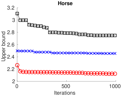
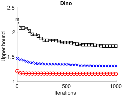
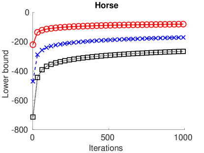
Figure 3: Upper (first row) and lower bounds (second row) generated in each iteration of the proposed algorithm. We test our method with $n_{p}$ value chosen as the ground truth and with different initial ranges $[\mathbf{r}_{gt}-\Delta,\mathbf{r}_{gt}+\Delta]$ of $\mathbf{r}$ and $[\mathbf{t}_{gt}-\Delta,\mathbf{t}_{gt}+\Delta]$ of $\mathbf{t}$, where $\mathbf{r}_{gt}$ (resp. $\mathbf{t}_{gt}$) denotes the ground truth $\mathbf{r}$ (resp. $\mathbf{t}$) solution. The margin $\Delta$ is respectively chosen as $0.5$, $1$ and $1.5$.

5.6 Branch-and-Bound

Based on the aforementioned preparations, we are now ready to employ the BnB algorithm to optimize $E$. The pseudocode is almost identical to Algo. 1 except that the initial hypercube $M$ is set as $\{(\mathbf{r},\mathbf{t})|\mathbf{r}\in\text{initial range of }\mathbf{r},\ \mathbf{t}\in\text{initial range of }\mathbf{t}\}$ and the notations $\mathbf{p}$, $\mathbf{p}^{k}$ and $\mathbf{p}^{k-1}$ are replaced by $\mathbf{P}$, $\mathbf{P}^{k}$ and $\mathbf{P}^{k-1}$, respectively.

In a similar vein as in Sec. 4.5, we rescale point sets $\mathscr{X}$ and $\mathscr{Y}$ to be unit sized and translate them to be centered at the origin before performing alignment. Unless otherwise stated, we set initial ranges for $\mathbf{r}$ and $\mathbf{t}$ as $\left[-\pi\mathbf{1}_{3},\pi\mathbf{1}_{3}\right]$ and $\left[-3\mathbf{1}_{3},3\mathbf{1}_{3}\right]$, respectively.

5.7 Convergence of the BnB algorithm

To evaluate the convergence of the proposed BnB algorithm, we use the separate outliers and inliers test described in Sec. 6.2.1 where the outlier to data ratio is chosen as $0.3$. The experimental result is presented in Fig. 3. Similar conclusion as in Sec. 4.6 can be drawn about the convergence of the proposed BnB algorithm in 3D case.

(a)

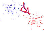
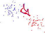
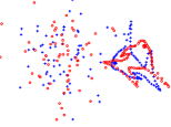
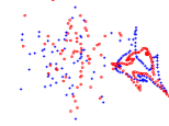
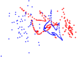
Figure 4: (a) to (c): model point sets and examples of scene piont sets in the deformation and noise tests, respectively. (d) to (i): examples of model and scene point sets in the mixed outliers and inliers test ((d), (e)), separate outliers and inliers test ((f), (g)) and occlusion+outlier test ((h), (i)), respectively. Here, the model points are marked by red circles and the scene points by blue crosses.

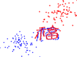
(a) RPM-HTB (simi)

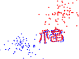
(b) RPM-HTB (aff)

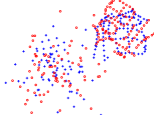
(c) RPM-PA (simi)

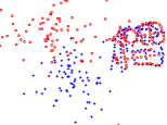
(d) RPM-CAV (simi)

(e) PR-GLS

Figure 5: Example of registration results by different methods in the separate outliers and inliers test, where $n_{p}$ is chosen as ground truth for all the methods.

6 Experiments

We implement the proposed algorithm (denoted as RPM-HTB) under Matlab R2020b and compare it with other methods on a computer with quad-core $3.5$ GHz CPUs. For the competing methods only outputting point correspondence, the generated point correspondence is used to compute the best affine transformation between two point sets. The matching error is defined as the root-mean-square distance between the transformed model inliers and their corresponding scene inliers. The maximum branching depth of RPM-HTB is chosen as $10$.

6.1 Case one: spatial transformation is linear w.r.t. its parameters

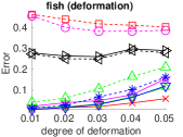
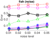
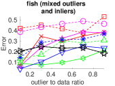
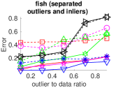
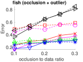
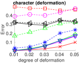
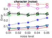
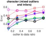
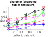
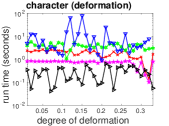
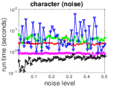
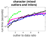
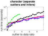
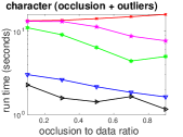
Figure 6: Average registration errors (top 2 rows) and run times (bottom row) by RPM-HTB, RPM-PA [5], RPM-CAV [4] and GLS under different $n_{p}$ values (chosen from $1/2$ to $1/1$ the ground truth value) over 100 random trials for the 2D deformation, noise, mixed outliers and inliers, separate outliers and inliers and occlusion+outlier tests. For the two types of outlier tests, only part of RPM-PA’s results is reported since RPM-PA requires too much memory when problem size is too big.

We compare with RPM-PA [5] and RPM-CAV [4], both of which are based on global optimization, can handle partial overlap and allow arbitrary similarity transformation between two point sets, making them good candidates for comparison. We also compare with PR-GLS [47], which is robust to outliers, rotation and occlusion.

2D similarity and affine transformations are respectively tested for RPM-HTB. For the former, we have

$$\mathbf{J}(\mathbf{x}_{i})=\begin{bmatrix}x_{i}^{1}&-x_{i}^{2}&1&0\\ x_{i}^{2}&x_{i}^{1}&0&1\end{bmatrix},\quad\mathbf{B}_{2}=\mathbf{B}([1,3,4],:)$$

For the latter, we have

$$\mathbf{J}(\mathbf{x}_{i})=\begin{bmatrix}x_{i}^{1}&x_{i}^{2}&0&0&1&0\\ 0&0&x_{i}^{1}&x_{i}^{2}&0&1\end{bmatrix},\quad\mathbf{B}_{2}=\mathbf{B}([1,2,5,8,11],:)$$

6.1.1 2D synthetic data

Synthetic data are easy to generate and can be used to test specific aspects of an algorithm. We perform 5 types of tests to evaluate a method’s robustness to various types of disturbances. i) Deformation test: The prototype shape is non-rigidly deformed to generate the scene set. ii) Noise test: The prototype shape is perturbed by positional noise to generate the scene point set. iii) Mixed outliers andinliers test: Random outliers are respectively superimposed on the prototype shape to generate the two point sets. iv) Separate outliers andinliers test: Random outliers are respectively added to different sides of the prototype shape to generate the two point sets. v) Occlusion+outlier test, First, the prototype shape is respectively occluded to generate the two point sets. Then, random outliers (outlier to data ratio is fixed to 0.5) are respectively added to different sides of the two point sets. Fig. 5 illustrates these tests. To evaluate a method’s ability at handling arbitrary rotation and scaling, random rotation and scaling within range $[0.5,1.5]$ are also performed when generating the two point sets. Fig. 5 shows examples of registration by different methods.

The registration errors by different methods are presented in the top 2 rows of Fig. 6. The results indicate that compared with other methods, RPM-HTB with $n_{p}$ value chosen as the ground truth are robust to deformation, noise and outliers in case when outliers are separate from inliers, but are not robust when outliers are mixed with inliers. This is because our method is not $\epsilon-$globally optimal as stated in Sec. 4.6, which affects our method’s robustness. PR-GLS performs poorly for almost all the tests. This is because our tests contain arbitrary rotations and PR-GLS is only a heuristic method. In terms of different transformation choices, affine transformation enables RPM-HTB to perform better for the deformation test, whereas similarity transformation enables RPM-HTB to perform better for the two types of outlier tests and the occlusion+outlier test. In terms of different choices of $n_{p}$ value, RPM-HTB with $n_{p}$ value close to the ground truth performs much better.

The average run times by different methods are presented in the bottom row of Fig. 6. RPM-HTB is only less efficient that the best performing method PR-GLS for the deformation and noise tests. It is almost as efficient as the best performing method RPM-CAV for the two types of outlier tests. In terms of different transformation choices, RPM-HTB employing similarity transformation is more efficient than it empolying affine transformation owing to similarity transformation’s less number of paramters.

From the two types of outlier tests, we can also see how different methods scale with problem size. RPM-HTB and RPM-CAV both scale the best with problem size, followed by PR-GLS and then RPM-PA.

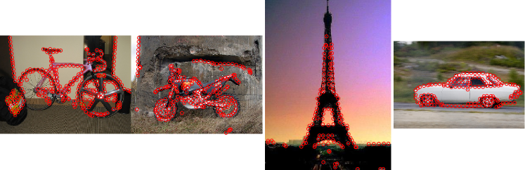
Figure 7: Model images with model point sets superimposed.

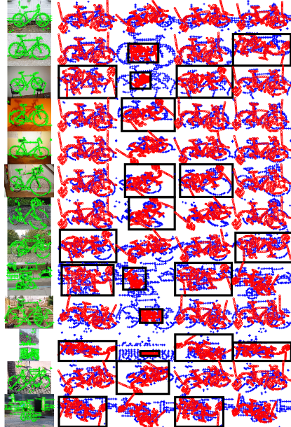
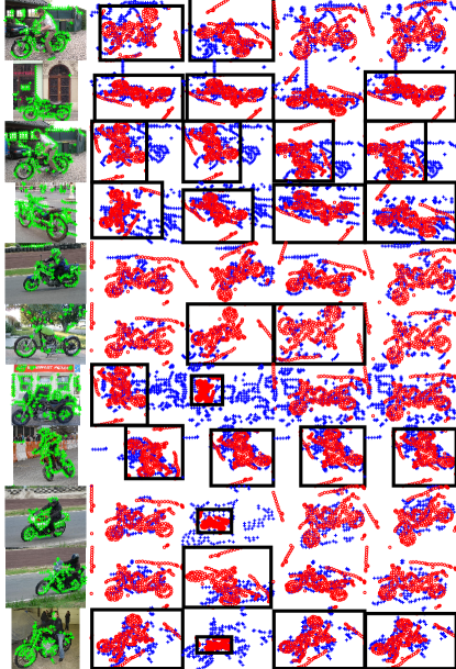
Figure 8: For each cell: scene images with scene point sets superimposed, registration results by RPM-HTB using similarity or affine transformations, RPM-PA [5] and RPM-CAV [4]. The $n_{p}$ value for each method is chosen as $0.9$ the minimum of the cardinalities of two point sets. The failure cases are encircled by black boxes.

6.1.2 2D real data

Point sets extracted from images constitute a more realistic type of data for evaluating registration methods. We use the Canny edge detector to extract 2D point sets from several images coming from the Caltech-256 [48] and VOC2007 [49] datasets. The extracted point sets are then used to test different registration methods, as illustrated in Fig. 7 and 8. To evaluate a method’s ability at handling arbitrary rotations, we rotate a model point set by $180^{\circ}$ before empolying a registration method to align it with a scene point set.

Since PR-GLS has high registration errors in the previous section, it is not tested. Fig. 8 reports the registration results by the remaining methods. RPM-HTB empolying similarity transformation, RPM-PA and RPM-CAV performs the best. RPM-HTB empolying affine transformation performs poorly. This is because affine transformation contains too much deformation freedom, causing the resulting registration method not robust to background clutters. Also, most of the methods fail in the car test. This is because the car test contains heavy background clutters, posing a serious challenge for the registration methods.

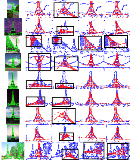
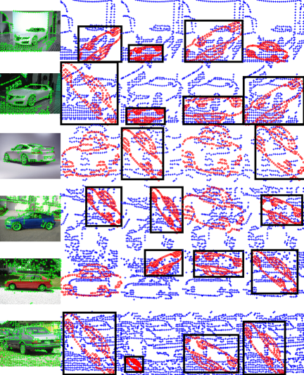
Figure 9:

6.2 Case two: 3D rigid transformation

Since RPM-PA and RPM-CAV are not efficient for the 3D case, they are not tested. Instead, we compare with Go-ICP [21], FRS [23], GORE [27] and TEASER++ [28], which are based on global optimization and allows arbitrary rigid transformation between two point sets, making them good candidates for comparison. For GORE and TEASER++, the FPFH feature descriptor is used to extract putative matches and the number of putative matches is set to 500.

6.2.1 3D synthetic data

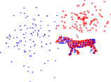
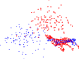
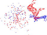
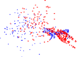
Figure 10: (a) to (c): model point sets and examples of scene point sets in the deformation and noise tests, respectively. (d) to (i): examples of model and scene point sets in the mixed outliers and inliers test ((d), (e)), separate outliers and inliers test ((f), (g)) and occlusion+outlier test ((h), (i)), respectively. Here, the model points are marked by red circles and the scene points by blue crosses.

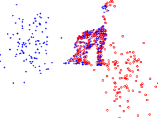
(a) RPM-HTB

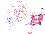
(b) Go-ICP

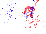
(c) FRS

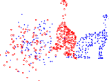
(d) GORE

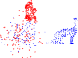
(e) TEASER++

Figure 11: Examples of registration results by different methods in the separate outliers and inliers test, where the $n_{p}$ values of RPM-HTB and Go-ICP are both chosen as the ground truth.

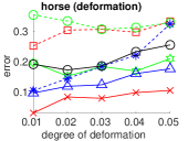
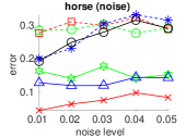
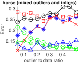
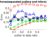
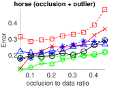
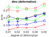
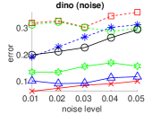
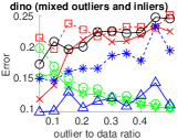
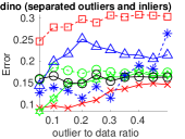
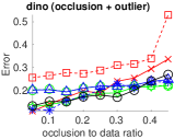
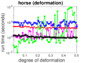
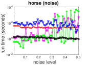
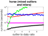
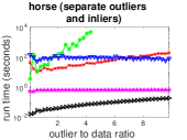
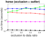
Figure 12: Average registration errors (top 2 rows) and run times (bottom row) of RPM-HTB and Go-ICP under different $n_{p}$ values (chosen from $1/2$ to $1/1$ the ground truth value), FRS, GORE and TEASER++ over 100 random trials for the 3D deformation, noise, mixed outliers and inliers, separate outliers and inliers and occlusion+outlier tests. For the two types of outlier tests, only part of FRS’s results is reported since FRS becomes too slow when problem size is too big.

Analogous to the experimental setup in Sec. 6.1, 5 types of tests are conducted to evaluate a method’s robustness to various types of disturbances: i) Deformation test, ii) Noise test, iii) Mixed outliers andinliers test, iv) Separate outliers andinliers testand v) Occlusion+outlier test, as is illustrated in Fig. 11. Examples of registration by different methods are shown in Fig. 11.

The registration errors by different methods are presented in the top 2 rows of Fig. 12. The results indicate that compared with other methods, RPM-HTB with $n_{p}$ value chosen as the ground truth is robust to deformation, noise and outliers in case when outliers are separate from inliers, but is not robust when outliers are mixed with inliers. In comparison, due to use of features, GORE and TEASER++ are not good at handling deformation, noise and outliers in case when outliers are mixed with inliers. In terms of different choices of $n_{p}$, RPM-HTB with $n_{p}$ value close to the ground truth performs much better.

The average run times by different methods are presented in the bottom row of Fig. 12. TEASER++ is the fastest, followed by Go-ICP and then RPM-HTB. GORE is slow in most instances. FRS quickly becomes inefficient when registration problem becomes challenging (e.g., when outliers increases in the two types of outlier tests).

From the two types of outlier tests, we can also see how different methods scale with problem size. Go-ICP and GORE scale the best with problem size, followed by TEASER++ and RPM-HTB. FRS scales the worst with problem size.

6.2.2 3DMatch dataset

3DMatch benchmark [50] contains scans of 62 scenaries coming from five existing RGB-D reconstruction datasets (sun3d, 7-scenes, rgbd-scenes-v2, bundlefusion and analysis-by-synthesis). D3Feat [51] provides a unified file structure and format recording the matching of these scenary scans. For sake of convenience, we use the scan pairs provided by D3Feat to evaluate performances of different methods. The matching errors by different methods are reported in Fig. 13. The results indicate that RPM-HTB performs overall better than Go-ICP and FRS, but worse than GORE and TEASER++. The good performances of GORE and TEASER++ partly comes from their use of features, which can significantly boost their abilities at matching complex structures. In comparison, the remaining methods only use point position information. Besides, the 3DMatch benchmark contains purely rigid transformations, which conforms well with the premises of GORE and TEASER++. Examples of registration by different methods are presented in Fig. 14.

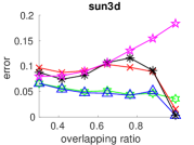
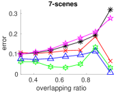
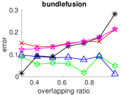
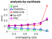
Figure 13: Average registration errors by different methods on the five RGB-D reconstruction datasets.

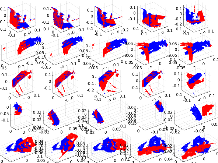
(a) GORE

(b) TEASER++

(c) RPM-HTB

(d) Go-ICP

(e) FRS

Figure 14: Examples of registration results generated by different methods on (from top to bottom) the five RGB-D reconstruction dataset: sun3d, 7-scenes, rgbd-scenes-v2, rgbd-scenes-v2 and analysis-by-synthesis.

6.2.3 Living room dataset

We use the large-scale field data contained in ”livingRoom.mat” from the MATLAB example ”3-D Point Cloud Registration and Stitching” to test performances of different methods. The dataset consists of a series of 3D point sets obtained by scanning a living room. All the points lie in a cube with an edge length of 4 metres. They were down-sampled with a gridsize of 0.2 metre.

Following [52], we use the following approach to get the ground-truth: We first use an ICP variant equipped with point-to-plane metric [53] to compute the rigid transformations between adjacent frames of point clouds. As the adjacent-frame point clouds differ only slightly, the transformations computed in this way can be regarded as the ground-truth. We then compute transformations between frames of point clouds in large separation by compositing adjacent-frame transformations. We next get ground-truth point correspondence by finding mutually nearest neighbors between the transformed model points and scene points.

Since the pose difference between adjacent frames is small, we set tighter initial range $\left[-\frac{\pi}{3}\mathbf{1}_{3},\frac{\pi}{3}\mathbf{1}_{3}\right]$ for $\mathbf{r}$ in our method so as to speed up convergence. The registration errors by different methods are reported in Fig. 15, where the $n_{p}$ value is chosen as $0.9$ the minimum of the cardinalities of two point sets for RPM-HTB and Go-ICP. Our method performs better than other methods, especially in the challenging cases where the frame separation is large. Examples of registration results by different methods are presented in Fig. 16. One can see that RPM-HTB is more robust to partial overlap than other methods.

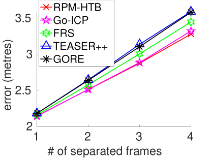
Figure 15: Average registration errors by different methods on the living room dataset.

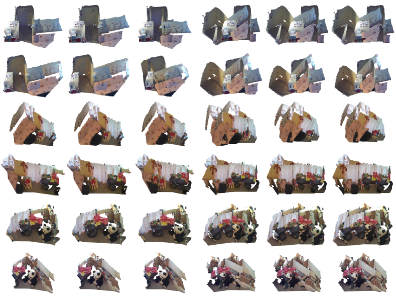
(a) ground-truth

(b) RPM-HTB

(c) Go-ICP

(d) FRS

(e) TEASER++

(f) GORE

Figure 16: Registration examples generated by different methods on the living room dataset.

7 Conclusion

In this paper, we presented a BnB based point set registration algorithm which can align partially overlapping point sets and can be rendered invariant to the corresponding transformation. The method has the merits that the lower bound can be efficiently computed via linear assignment and the dimensionality of the branching space equals the number of transformation parameters. These merits enable the method to be computationally efficient and scale well with problem size. The use of the BnB algorithm enables the proposed method to be robust to non-rigid deformations, positional noise and outliers in case when outliers are not mixed with inliers when compared with the state-of-the-art approaches.

Nevertheless, the proposed method can only tackle transformations with few parameters due to exponential complexity of the proposed BnB algorithm with respect to the dimensionality of the branching space. Besides, the method’s robustness is substantially impacted by the parameter setting for $n_{p}$. This is because branching depth instead of duality gap is adopted as the stopping criterion for the proposed method due to slow convergence of the duality gap. In the future, we will explore better methods capable of generating tighter lower bounds. We will also develope adaptive $n_{p}$ setting scheme.

ACKNOWLEDGMENTS

This work was supported by National Natural Science Foundation of China under Grants 61773002 and U19A2073, the Fundamental Research Program of Shanxi Province, China under Grant 202103021223381 and Scientific and Technological Innovation Programs of Higher Education Institutions in Shanxi Province, China under Grant 2022L517.

Appendix A Convergence properties of bilinear and trilinear monomials

Proposition 3

Assume $\underline{x}\leq x\leq\overline{x}$ and $\underline{y}\leq y\leq\overline{y}$, if $|\overline{x}-\underline{x}|$ or $|\overline{y}-\underline{y}|$ is sufficiently small, then we will have $|xy-(xy)_{l}|\leq\epsilon$ for any real number $\epsilon>0$.

Proof: Since

$$(xy)_{l} \triangleq\frac{1}{2}\sum_{i}(xy)_{li}=\frac{1}{2}(\underline{x}+\overline{x})y+\frac{1}{2}(\underline{y}+\overline{y})x-\frac{1}{2}(\underline{x}\underline{y}+\overline{x}\overline{y})$$ (28)

It follows that

$$|xy-(xy)_{l}| =\frac{1}{2}\left|(x-\underline{x})(y-\underline{y})+(\overline{x}-x)(\overline{y}-y)\right|$$

$$\leq\frac{1}{2}|(x-\underline{x})(y-\underline{y})|+\frac{1}{2}|(\overline{x}-x)(\overline{y}-y)|$$

$$\leq|\overline{x}-\underline{x}|\cdot|\overline{y}-\underline{y}|$$ (29)

Therefore, if $|\overline{x}-\underline{x}|$ or $|\overline{y}-\underline{y}|$ is sufficiently small, we will have $|xy-(xy)_{l}|\leq\epsilon$ for any $\epsilon>0$.

Proposition 4

Assume $\underline{x}\leq x\leq\overline{x}$, $\underline{y}\leq y\leq\overline{y}$ and $\underline{z}\leq z\leq\overline{z}$, if the ranges of any two variables that makes up $xyz$ are sufficiently small, we will have $|xyz-(xyz)_{l}|\leq\epsilon$ for any real number $\epsilon>0$.

Proof: In the case $\underline{x}\leq 0,\underline{y}\geq 0,\underline{z}\leq 0,\overline{z}\geq 0$, we have the following inequalities (which has been presented in Sec. 3.2 of the main paper):

$$(xyz)_{l1}\triangleq \overline{y}\overline{z}x+\overline{x}\overline{z}y+\overline{x}\overline{y}z-2\overline{x}\overline{y}\overline{z}\leq xyz$$ (30)

$$(xyz)_{l2}\triangleq \overline{y}\underline{z}x+\underline{x}\overline{z}y+\underline{x}\overline{y}z-\underline{x}\overline{y}\underline{z}-\underline{x}\overline{y}\overline{z}\leq xyz$$ (31)

$$(xyz)_{l3}\triangleq \overline{y}\underline{z}x+\underline{x}\underline{z}y+\underline{x}\underline{y}z-\underline{x}\overline{y}\underline{z}-\underline{x}\underline{y}\underline{z}\leq xyz$$ (32)

$$(xyz)_{l4}\triangleq \underline{y}\overline{z}x+\overline{x}\underline{z}y+\overline{x}\underline{y}z-\overline{x}\underline{y}\overline{z}-\overline{x}\underline{y}\underline{z}\leq xyz$$ (33)

$$(xyz)_{l5}\triangleq \underline{y}\underline{z}x+\overline{x}\underline{z}y+\underline{x}\underline{y}z-\overline{x}\underline{y}\underline{z}-\underline{x}\underline{y}\underline{z}\leq xyz$$ (34)

$$(xyz)_{l6}\triangleq \underline{y}\overline{z}x+\underline{x}\overline{z}y+\phi/(\overline{z}-\underline{z})z-\phi\underline{z}/(\overline{z}-\underline{z})$$

$$-\underline{x}\overline{y}\overline{z}-\overline{x}\underline{y}\overline{z}+\overline{x}\overline{y}\underline{z}\leq xyz$$ (35)

where $\phi=\underline{x}\overline{y}\overline{z}-\overline{x}\overline{y}\underline{z}-\underline{x}\underline{y}\overline{z}+\overline{x}\underline{y}\overline{z}$.

For the first inequality (30), we have

$$|xyz-(xyz)_{l1}| =\left|xz(y-\overline{y})+x\overline{y}(z-\overline{z})+\overline{x}\overline{z}(\overline{y}-y)+\overline{x}\overline{y}(\overline{z}-z)\right|$$

$$\leq|xz(y-\overline{y})|+|x\overline{y}(z-\overline{z})|+|\overline{x}\overline{z}(\overline{y}-y)|+|\overline{x}\overline{y}(\overline{z}-z)|$$ (36)

Therefore, if $|\overline{y}-\underline{y}|$ and $|\overline{z}-\underline{z}|$ are sufficiently small, we will have $|xyz-(xyz)_{l1}|\leq\epsilon$.

Similarly, we can prove

$$|xyz-(xyz)_{l1}|\leq|xz(y-\overline{y})|+|\overline{y}z(x-\overline{x})|+|\overline{y}\overline{z}(\overline{x}-x)|+|\overline{x}\overline{z}(\overline{y}-y)|$$ (37)

Therefore, if $|\overline{x}-\underline{x}|$ and $|\overline{y}-\underline{y}|$ are sufficiently small, we will have $|xyz-(xyz)_{l1}|\leq\epsilon$.

Similarly, one can also prove

$$|xyz-(xyz)_{l1}|\leq|xy(z-\overline{z})|+|y\overline{z}(x-\overline{x})|+|\overline{y}\overline{z}(\overline{x}-x)|+|\overline{x}\overline{y}(\overline{z}-z)|$$ (38)

Therefore, if $|\overline{x}-\underline{x}|$ and $|\overline{z}-\underline{z}|$ are sufficiently small, we will have $|xyz-(xyz)_{l1}|\leq\epsilon$.

In conclusion, we will have $|xyz-(xyz)_{l1}|\leq\epsilon$ if the ranges of any two variables that makes up $xyz$ are sufficiently small. For other inequalities (31) to (35), we can prove similar results.

Based on the above results, therefore, for the average of the inequalities (30) to (35), we will have $|xyz-(xyz)_{l}|\leq\epsilon$ if the ranges of any two variables are sufficiently small.

For other cases of the bounds on $x,y,z$, we can prove similar results.

Appendix B Derivation of Eq. (15) in the main text

Based on Eq. (3), given a feasible $\mathbf{p}$, $E$ is apparently a convex quadratic function of $\boldsymbol{\theta}$. Thus, the optimal $\boldsymbol{\theta}$ minimizing $E$ can be obtained by solving the equation $\frac{\partial E}{\partial\boldsymbol{\theta}}=0$, where for convenient, we choose Eq. 6 as the form of $E$. Consequently, the optimal $\boldsymbol{\theta}$ can be obtained as:

$$\boldsymbol{\hat{\theta}}=\left[\text{mat}(\mathbf{K}\mathbf{B}_{2}\mathbf{p}){+}\mathbf{C}\right]^{-1}\mathbf{A}\mathbf{p}$$ (39)

By substituting $\boldsymbol{\hat{\theta}}$ into Eq. 6, $\boldsymbol{\theta}$ is eliminated and we get an energy function in only one variable $\mathbf{p}$ as shown in Eq. 15.

References

- [1] H. Chui, A. Rangarajan, A new point matching algorithm for non-rigid registration, Computer Vision and Image Understanding 89 (2-3) (2003) 114–141.
- [2] W. Lian, L. Zhang, M.-H. Yang, An efficient globally optimal algorithm for asymmetric point matching, IEEE Transactions on Pattern Analysis and Machine Intelligence 39 (7) (2017) 1281–1293.
- [3] W. Lian, L. Zhang, Point matching in the presence of outliers in both point sets: A concave optimization approach, in: IEEE Conference on Computer Vision and Pattern Recognition, 2014, pp. 352–359.
- [4] W. Lian, L. Zhang, A concave optimization algorithm for matching partially overlapping point sets, Pattern Recognition 103 (2020) 107322. doi:https://doi.org/10.1016/j.patcog.2020.107322.
- [5] W. Lian, W. Zuo, Z. Cui, A polyhedral annexation algorithm for aligning partially overlapping point sets, IEEE Access 9 (2021) 166750–166761. doi:10.1109/ACCESS.2021.3135863.
-
[6]
J. Ma, X. Jiang, A. Fan, J. Jiang, J. Yan,
Image matching from
handcrafted to deep features: A survey, Int. J. Comput. Vision 129 (1)
(2021) 23?79.
doi:10.1007/s11263-020-01359-2.
URL https://doi.org/10.1007/s11263-020-01359-2 - [7] P. J. Besl, N. D. McKay, A method for registration of 3-d shapes, IEEE Trans. Pattern Analysis and Machine Intelligence 14 (2) (1992) 239–256.
- [8] C. Zhang, S. Du, J. Liu, Y. Li, J. Xue, Y. Liu, Robust iterative closest point algorithm with bounded rotation angle for 2d registration, Neurocomputing 195 (2016) 172–180.
- [9] L. Liang, Precise iterative closest point algorithm for rgb-d data registration with noise and outliers, Neurocomputing 399 (2020) 361–368.
- [10] M. Sofka, G. Yang, C. V. Stewart, Simultaneous covariance driven correspondence (cdc) and transformation estimation in the expectation maximization framework, in: IEEE Conf. Computer Vision and Pattern Recognition, 2007, pp. 1–8.
- [11] J. Ma, W. Qiu, J. Zhao, Y. Ma, A. L. Yuille, Z. Tu, Robust estimation of transformation for non-rigid registration, IEEE Transactions on Signal Processing 63 (5) (2015) 1115–1129. doi:10.1109/TSP.2014.2388434.
- [12] A. Myronenko, X. Song, Point set registration: Coherent point drift, IEEE Transactions on Pattern Analysis and Machine Intelligence 32 (12) (2010) 2262–2275.
- [13] B. Jian, B. C. Vemuri, Robust point set registration using gaussian mixture models, IEEE Trans. Pattern Analysis and Machine Intelligence 33 (8) (2011) 1633–1645.
- [14] D. Campbell, L. Petersson, An adaptive data representation for robust point-set registration and merging, in: 2015 IEEE International Conference on Computer Vision (ICCV), 2015, pp. 4292–4300. doi:10.1109/ICCV.2015.488.
- [15] W. Gao, R. Tedrake, Filterreg: Robust and efficient probabilistic point-set registration using gaussian filter and twist parameterization, in: 2019 IEEE/CVF Conference on Computer Vision and Pattern Recognition (CVPR), 2019, pp. 11087–11096. doi:10.1109/CVPR.2019.01135.
- [16] F. J. Lawin, M. Danelljan, F. S. Khan, P.-E. Forssen, M. Felsberg, Density adaptive point set registration, in: 2018 IEEE/CVF Conference on Computer Vision and Pattern Recognition, 2018, pp. 3829–3837. doi:10.1109/CVPR.2018.00403.
- [17] B. Eckart, K. Kim, J. Kautz, Hgmr: Hierarchical gaussian mixtures for adaptive 3d registration, in: European Conference on Computer Vision, Springer International Publishing, 2018, pp. 730–746.
- [18] J. Ma, J. Zhao, A. L. Yuille, Non-rigid point set registration by preserving global and local structures, IEEE Transactions on Image Processing 25 (1) (2016) 53–64. doi:10.1109/TIP.2015.2467217.
- [19] H. Li, R. Hartley, The 3d-3d registration problem revisited, in: International Conference on Computer Vision, 2007.
- [20] C. Olsson, F. Kahl, M. Oskarsson, Branch-and-bound methods for euclidean registration problems, IEEE Transactions on Pattern Analysis and Machine Intelligence 31 (5) (2009) 783–794.
- [21] J. Yang, H. Li, D. Campbell, Y. Jia, Go-icp: A globally optimal solution to 3d icp point-set registration, IEEE Transactions on Pattern Analysis and Machine Intelligence 38 (11) (2016) 2241–2254. doi:10.1109/TPAMI.2015.2513405.
- [22] D. Campbell, L. Petersson, Gogma: Globally-optimal gaussian mixture alignment, in: The IEEE Conference on Computer Vision and Pattern Recognition, 2016.
- [23] Á. Parra, T.-J. Chin, A. Eriksson, H. Li, D. Suter, Fast rotation search with stereographic projections for 3d registration, IEEE Transactions on Pattern Analysis and Machine Intelligence 38 (11) (2016) 2227–2240.
- [24] Y. Liu, C. Wang, Z. Song, M. Wang, Efficient global point cloud registration by matching rotation invariant features through translation search, in: European Conference on Computer Vision, 2018, pp. 448–463.
- [25] J. Straub, T. Campbell, J. P. How, J. W. Fisher, Efficient global point cloud alignment using bayesian nonparametric mixtures, in: 2017 IEEE Conference on Computer Vision and Pattern Recognition (CVPR), 2017, pp. 2403–2412. doi:10.1109/CVPR.2017.258.
- [26] Q.-Y. Zhou, J. Park, V. Koltun, Fast global registration, in: European Conference on Computer Vision, Springer International Publishing, Cham, 2016, pp. 766–782.
- [27] Á. Parra, T.-J. Chin, Guaranteed outlier removal for point cloud registration with correspondences, TPAMI 40 (12) (2018) 2868–2882.
- [28] H. Yang, J. Shi, L. Carlone, Teaser: Fast and certifiable point cloud registration, IEEE Transactions on Robotics (2020) 1–20doi:10.1109/TRO.2020.3033695.
- [29] R. Q. Charles, H. Su, M. Kaichun, L. J. Guibas, Pointnet: Deep learning on point sets for 3d classification and segmentation, in: 2017 IEEE Conference on Computer Vision and Pattern Recognition (CVPR), 2017, pp. 77–85. doi:10.1109/CVPR.2017.16.
- [30] Y. Aoki, H. Goforth, R. A. Srivatsan, S. Lucey, Pointnetlk: Robust and efficient point cloud registration using pointnet, in: 2019 IEEE/CVF Conference on Computer Vision and Pattern Recognition (CVPR), 2019, pp. 7156–7165. doi:10.1109/CVPR.2019.00733.
- [31] X. Huang, G. Mei, J. Zhang, Feature-metric registration: A fast semi-supervised approach for robust point cloud registration without correspondences, in: Proceedings of the IEEE/CVF Conference on Computer Vision and Pattern Recognition (CVPR), 2020.
- [32] C. Choy, J. Park, V. Koltun, Fully convolutional geometric features, in: 2019 IEEE/CVF International Conference on Computer Vision (ICCV), 2019, pp. 8957–8965. doi:10.1109/ICCV.2019.00905.
- [33] Z. Gojcic, C. Zhou, J. D. Wegner, W. Andreas, The perfect match: 3d point cloud matching with smoothed densities, in: International conference on computer vision and pattern recognition (CVPR), 2019.
- [34] C. Choy, W. Dong, V. Koltun, Deep global registration, in: CVPR, 2020.
- [35] K. Musgrave, S. Belongie, S.-N. Lim, A metric learning reality check, in: A. Vedaldi, H. Bischof, T. Brox, J.-M. Frahm (Eds.), Computer Vision – ECCV 2020, Springer International Publishing, Cham, 2020, pp. 681–699.
- [36] Y. Wang, J. Solomon, Deep closest point: Learning representations for point cloud registration, in: 2019 IEEE/CVF International Conference on Computer Vision (ICCV), 2019, pp. 3522–3531. doi:10.1109/ICCV.2019.00362.
-
[37]
Y. Wang, Y. Sun, Z. Liu, S. E. Sarma, M. M. Bronstein, J. M. Solomon,
Dynamic graph cnn for learning on
point clouds, ACM Trans. Graph. 38 (5).
doi:10.1145/3326362.
URL https://doi.org/10.1145/3326362 - [38] A. Vaswani, N. Shazeer, N. Parmar, J. Uszkoreit, L. Jones, A. N. Gomez, u. Kaiser, I. Polosukhin, Attention is all you need, in: Proceedings of the 31st International Conference on Neural Information Processing Systems, NIPS’17, Curran Associates Inc., Red Hook, NY, USA, 2017, pp. 6000–6010.
-
[39]
Y. Wang, J. M. Solomon,
Prnet:
Self-supervised learning for partial-to-partial registration, in: Advances
in Neural Information Processing Systems, Vol. 32, Curran Associates, Inc.,
2019.
URL https://proceedings.neurips.cc/paper/2019/file/ebad33b3c9fa1d10327bb55f9e79e2f3-Paper.pdf - [40] J. Li, C. Zhang, Z. Xu, H. Zhou, C. Zhang, Iterative distance-aware similarity matrix convolution with mutual-supervised point elimination for efficient point cloud registration, in: Computer Vision–ECCV 2020: 16th European Conference, Glasgow, UK, August 23–28, 2020, Proceedings, Part XXIV 16, Springer, 2020, pp. 378–394.
- [41] Y. Shen, L. Hui, H. Jiang, J. Xie, J. Yang, Reliable inlier evaluation for unsupervised point cloud registration, in: Proceedings of the AAAI Conference on Artificial Intelligence, Vol. 36, 2022, pp. 2198–2206.
- [42] Y. Shu, Z. Hou, B. Xiao, X. Bi, X. Luan, W. Li, Partial-to-partial point cloud registration based on multi-level semantic-structural cognition, in: 2022 IEEE International Conference on Multimedia and Expo (ICME), IEEE, 2022, pp. 1–6.
- [43] L. Gorelick, Y. Boykov, O. Veksler, I. B. Ayed, A. Delong, Submodularization for quadratic pseudo-boolean optimization, in: CVPR, 2014.
- [44] M. Chandraker, D. Kriegman, Globally optimal bilinear programming for computer vision applications, in: 2008 IEEE Conference on Computer Vision and Pattern Recognition, 2008, pp. 1–8. doi:10.1109/CVPR.2008.4587846.
- [45] C. Meyer, C. Floudas, Trilinear monomials with positive or negative domains: facets of the convex and concave envelopes, 2003, pp. 327–352.
- [46] C. Meyer, C. Floudas, Trilinear monomials with mixed sign domains: Facets of the convex and concave envelopes, Journal of Global Optimization 29 (2004) 125–155. doi:10.1023/B:JOGO.0000042112.72379.e6.
- [47] J. Ma, J. Zhao, A. L. Yuille, Non-rigid point set registration by preserving global and local structures, IEEE Transactions on Image Processing 25 (1) (2016) 53–64. doi:10.1109/TIP.2015.2467217.
- [48] G. Griffin, A. Holub, P. Perona, Caltech-256 object category dataset, technical report, California Inst. of Technology (2007).
- [49] M. Everingham, L. Van Gool, C. K. I. Williams, J. Winn, A. Zisserman, The PASCAL Visual Object Classes Challenge 2007 (VOC2007) Results, http://www.pascal-network.org/challenges/VOC/voc2007/workshop/index.html.
- [50] A. Zeng, S. Song, M. Nießner, M. Fisher, J. Xiao, T. Funkhouser, 3dmatch: Learning local geometric descriptors from rgb-d reconstructions, in: CVPR, 2017.
- [51] L. Z. H. F. L. Q. Xuyang Bai, Zixin Luo, C.-L. Tai, D3feat: Joint learning of dense detection and description of 3d local features, arXiv:2003.03164 [cs.CV].
- [52] W. Lian, J. Zuo, Z. Ding, Low-rank path-following algorithm for 3d similarity registration, IET Computer Vision 13 (4) (2019) 404–410.
- [53] Y. Chen, G. Medioni, Object modeling by registration of multiple range images, in: IEEE International Conference on Robotics and Automation, 1991, pp. 2724–2729.