Learning Successor States and Goal-Dependent Values: A Mathematical Viewpoint

Abstract

In reinforcement learning, temporal difference-based algorithms can be sample-inefficient: for instance, with sparse rewards, no learning occurs until a reward is observed. This can be remedied by learning richer objects, such as a model of the environment, or successor states. Successor states model the expected future state occupancy from any given state (Dayan, 1993; Kulkarni et al., 2016), and summarize all paths in the environment for a given policy. They are related to goal-dependent value functions, which learn how to reach arbitrary states.

We formally derive the temporal difference algorithm for successor state and goal-dependent value function learning, either for discrete or for continuous environments with function approximation. Especially, we provide finite-variance estimators even in continuous environments, where the reward for exactly reaching a goal state becomes infinitely sparse.

Successor states satisfy more than just the Bellman equation: a backward Bellman operator and a Bellman–Newton (BN) operator encode path compositionality in the environment. The BN operator is akin to second-order gradient descent methods, and provides the “true” update of the value function when acquiring more observations from the environment, with explicit tabular bounds. In the tabular case and with infinitesimal learning rates, mixing the usual and backward Bellman operators provably improves eigenvalues for asymptotic convergence, and the asymptotic convergence of the BN operator is provably better than TD, with a rate independent from the environment. However, the BN method is more complex and less robust to sampling noise.

Finally, a forward-backward (FB) finite-rank parameterization of successor states enjoys reduced variance and improved samplability, provides a direct model of the value function, has fully understood fixed points corresponding to long-range dependencies (but ignores small-scale dependencies), approximates the BN method, and provides two canonical representations of states as a byproduct.

1 Introduction, Overview of Results

The successor state operator of a Markov reward process is an object that directly encodes the passage from a reward function to the corresponding value function. In particular, it expresses the value functions of all possible reward functions for a given, fixed policy.

Goal-dependent value functions are a related object with many similar properties. They describe the optimal value functions and policies for a specific set of tasks: typically, for all rewards located at all possible target states. In this case, the policy depends on the target state.

Here we offer a formal treatment of these objects in both finite and continuous spaces. We present several learning algorithms and associated results. In particular, we focus on proper treatment of the infinitely-sparse reward problem encountered by TD-style approaches in continuous spaces if the reward is located at a precise state.

Possible advantages of working with these objects include:

• Contrary to TD, learning starts even before any rewards are observed. Sucessor state learning extracts information from every observed transition, by learning how to reach every visited state. Subsequent reward observations provide an instantaneous update to the value function via the successor state operator.

  This learning is done without reward signals, illustrating an “unsupervised reinforcement learning” approach. Successor state lie in between model-free and model-based reinforcement learning approaches, providing a representation of the future of a state without having to synthesize future states or unrolling synthetic trajectories. Algorithmically, they rely on having two states as inputs rather than generating a state.

• Successor states and goal-dependent values exploit relationships between how to reach different states. With function approximation, generalization occurs between different target states. But even in a tabular setting with no generalization, these objects satisfy more algebraic relations than the usual Bellman equation: a backward Bellman equation and a Bellman–Newton equation, expressing path compositionality in the Markov process (Fig 1). This leads to quantifiable asymptotic gains.

• Successor states and goal-dependent values can be used to solve several problems at once, such as learning to reach arbitrary states. Even for optimizing a single reward, they can be used for auxiliary tasks such as going to an arbitrary state, which could be useful for exploration, or to provide good state representations.

For learning value functions dependent on goal states, an obvious approach is to apply any standard reinforcement learning algorithm, with reward $1$ when the visited state is equal to the goal state (e.g., (Schaul et al., 2015)). But this breaks down in continuous spaces, as the reward function becomes infinitely sparse (a random trajectory is never going to reach any predefined goal exactly). Even in discrete spaces, the reward becomes exponentially sparse as the number of components increase.

This problem is avoided by a suitable mathematical treatment. The intuition behind several of our results is the following: If the goal is to learn how to reach arbitrary states, then this is not a sparse reward problem, although straightforward TD implementations treat it as such; it is a problem with rewards everywhere. Approaches such as hindsight experience replay (Andrychowicz et al., 2017) attempt to exploit this intuition by resampling goals a posteriori in an off-policy algorithm, but it is unclear to us how much of the problem HER solves in continuous spaces. The mathematical treatment here proves that finite-variance algorithms exist for such problems, even in continuous spaces.

Overview of results.

In a nutshell, successor states summarize all possible paths in the environment for a given policy (Section 4.3). For finite spaces, the entries $M_{ss^{\prime}}$ of the successor state matrix describe the expected discounted time spent in state $s^{\prime}$ by a trajectory starting at $s$ (Dayan, 1993): $M_{ss^{\prime}}=\mathbb{E}\left[\sum_{t\geqslant 0}\gamma^{t}\mathbbm{1}_{s_{t}=s^{\prime}}|s_{0}=s\right]$. The entry $M_{ss^{\prime}}$ is also the value function at $s$ if the reward is $1$ at $s^{\prime}$ and $0$ everywhere else. As such, $M$ contains the information about reaching every state in the environment, not just those states providing a reward. For a fixed policy, the value function depends linearly on the reward: in a finite state space, for any reward function, represented as a vector $R$ over states, its associated value function is $V=MR$.

The goal-dependent value function $V_{ss^{\prime}}$ at state $s$ for goal $s^{\prime}$ (another state) is defined as the value function at $s$ of the optimal policy for reaching a unit reward located at $s^{\prime}$. The difference with $M_{ss^{\prime}}$ is now that the policy depends on $s^{\prime}$ instead of being fixed. Learning this object allows for learning how to reach different goal states. Contrary to $M_{ss^{\prime}}$, $V_{ss^{\prime}}$ does not contain information on how to optimize dense rewards (mixtures of goal states), only rewards located at a single state. It is also possible to define $V$ for more general types of goals rather just a target state, although the goals must be predefined and mixtures of goals are not possible a posteriori.

The bulk of the text presents theoretically well-motivated algorithms to learn these objects directly for any two states $s,s^{\prime}$. The main contributions of this text are the following.

• We formally define successor states and goal-dependent value (and $Q$) functions in general state spaces (Sections 3 and 5), extending the discrete case of (Dayan, 1993). For continuous states, this involves some measure theory (Section 3.2), but the intuition is clear from the discrete case (Section 3.1).

  Successor states are always well-defined for a given policy (Theorem 2). But goal-dependent value functions are generally not unique in continuous spaces (Section 5.3); still, there exists a canonical solution (Theorem 14), smaller than all others.

• We formally derive the temporal difference (TD) algorithm for successor state learning, both for discrete spaces, and for continuous spaces with function approximation (Theorem 6), beyond the tabular setting of (Dayan, 1993). A naive application of TD on a state-goal product space, with reward $1$ when the state reaches the goal, degenerates in continuous spaces: the reward becomes infinitely sparse (it is $0$ with probability $1$ and $\infty$ with probability $0$). Instead, the TD estimators we provide have finite variance (Section 4.1.4, Proposition 8).

  Known convergence results for TD extend to this setting: tabular case with any sampling policy, linear parameterization on-policy, arbitrary function approximation assuming reversibility of the Markov process (Section 4.1.5).

  Likewise, we formally derive the TD algorithm for goal-dependent $Q$ and $V$ functions (Section 5), with finite-variance estimators even in continuous spaces. The goals may be target states, or target values for some vector-valued function of the states (Section 5.2).

• Algorithmically, successor states and goal-dependent values are represented by function approximators depending on two states (the current state and a goal state) instead of one. TD learning works in a black-box environment by sampling from a set of observed transitions $s\to s^{\prime}$ between states, and sampling goal states (typically from the same distribution). No reward signal is needed.

  Most variants of TD still apply: $V$ or $Q$ learning, target networks, multi-step returns… (Appendix A). Notably, Appendix A.6 describes relative TD to deal directly with a decay factor $\gamma=1$ and to reduce variance for $\gamma$ close to $1$.

  Successor states and goal-dependent values can be used to learn an optimal policy for a particular reward, or to learn goal-dependent policies. Many different options are described in Section 8, such as $Q$-learning or policy gradient, with several ways to learn the value function from successor states.

• Successor states satisfy more than one Bellman equation: we introduce backward TD for successor states (Section 4.2, Theorem 9), and the corresponding parametric update (Theorem 26, Appendix A.4).

  Successor states encode all paths in the Markov process for a fixed policy (Section 4.3). The usual (forward) Bellman equation $M=\operatorname{Id}+\gamma PM$ adds a newly observed transition at the front of all known paths, while the backward Bellman equation $M=\operatorname{Id}+\gamma MP$ extends known paths by adding newly observed transitions at the back. This backward equation exists for successor states but not goal-dependent value functions. In the tabular setting and with small learning rates, combining forward and backward TD turns out to improve the eigenvalues of the learning process (Section 9.2).

• We introduce “second-order” methods for learning successor states, which are to TD what Newton-type methods are to first-order gradient descent (Section 7). In addition to the usual (forward) and the backward Bellman equations, there is a third Bellman equation satisfied by $M$, which leads to the Bellman–Newton operator $M\leftarrow 2M-M^{2}+\gamma MPM$ (Section 7.2). It also enjoys a path interpretation, learning by path concatenation and doubling the length of known paths (Proposition 20). The forward and backward Bellman operators only increase the length of known paths by $1$ (Appendix C).

  Asymptotically and in the small learning rate limit, the Bellman–Newton operator converges provably faster than TD (Section 9.3), with an asymptotic rate independent of the environment and policy. However, in practice this method is less resistant to sample noise: smaller learning rates are necessary, so the comparison with TD is less clear. There is also a parametric version of the Bellman–Newton operator (Theorem 21), but it is numerically fickle.

  We also study the estimation of $M$ by direct inversion of $\operatorname{Id}-\gamma\hat{P}$ using an empirical estimate $\hat{P}$ of the transition matrix $P$ in a finite state space. The resulting update of $M$ when adding each new observation is the same as a Bellman–Newton update with learning rate $1/t$ (Theorems 17 and 18). In finite spaces, we provide an explicit non-asymptotic bound for the convergence of $M$ and the value function $V$ based on these empirical estimates (Theorem 16).

• Representing the successor state operator as a dot product $F(s_{1})^{\!\top}\!B(s_{2})$ between features of the starting state $s_{1}$ and the target state $s_{2}$ has many nice properties (Section 6). Here, the “forward” and “backward” feature functions $F$ and $B$ are both learned to approximate $M$: this may have independent interest for representation learning.

  First, this method provides a direct representation of the value function without additional learning (Eq. 47).

  Second, when learning $F$ and $B$ by any of the algorithms above, in expectation the updates factorize between $s_{1}$ and $s_{2}$ (Proposition 15). This allows for variance reduction, and for purely trajectory-wise algorithms which only use the currently observed transition $s\to s^{\prime}$ without sampling an additional target state $s_{2}$ (Section 6.2), in contrast to the general form of TD for $M$.

  Third, this representation keeps some properties of the Bellman–Newton method without its shortcomings; they actually coincide when the transition matrix of the process is symmetric (Theorem 41).

  Finally, the fixed points of TD for this representation can be fully characterized in the tabular and overparameterized cases (Propositions 35–39 in Appendix E, and Section 6.2). They are related to eigenspaces of the transition matrix $P$. Notably, in the tabular or overparameterized case, if forward TD is used to learn $F$ and backward TD to learn $B$, then the fixed points are exactly local minimizers of the error between the $F^{\!\top}\!B$ model and the true successor state operator (Proposition 35). In contrast, for ordinary TD on the value function and a linear model, the fixed points are not minimizers of the error to the true value function.

Some related work on successor states.

The successor state operator is linked to various existing objects under various names (fundamental matrix, occupation matrix, successor representations, successor features…). Successor states have even been identified in the neurosciences (Stachenfeld et al., 2017).

For discount factor $\gamma=1$, the successor matrix $M$ is known as the fundamental matrix (Kemeny and Snell, 1960; Brémaud, 1999; Grinstead and Snell, 1997) of a Markov process (up to subtracting the invariant measure). The fundamental matrix encodes many properties of the Markov chain, such as value functions ((Bertsekas, 2012), as we use here) or hitting times (Kemeny and Snell, 1960). In a reinforcement learning context, and with $\gamma<1$, this matrix goes back at least to (Dayan, 1993).

Learning successor states by temporal difference is mentioned in (Dayan, 1993) for the tabular case and with linear approximations; the parametric case has never been derived as far as we know.

In a deep learning context, several recent works have used the related successor representations (Kulkarni et al., 2016), e.g., for transfer (Barreto et al., 2017; Borsa et al., 2018; Zhang et al., 2017; Lehnert et al., 2017; Ma et al., 2018; Barreto et al., 2020), hierarchical RL (Machado et al., 2018) or exploration (Machado et al., 2019).

In particular, the Deep Successor Representation algorithm (Kulkarni et al., 2016) approximates successor states by learning a state representation $\varphi(s)$ together with a successor representation $m(s)$ defined as the expected discounted representation of future states from $s$: $m(s)=\mathbb{E}\left[\sum_{t\geqslant 0}\gamma^{t}\varphi(s_{t})|s_{0}=s\right]$. As $\varphi=m=0$ is a fixed point of the method, a reconstruction loss must be used to prevent collapse. Here we directly learn the successor states $M_{ss^{\prime}}$ for every pair of states in the original space.

Successor states provide the value function for every goal state: this is related to learning multiple RL tasks (Sutton et al., 2011; Schaul et al., 2015; Jin et al., 2020; Pinto and Gupta, 2017) which performs joint $V$- or $Q$-learning for a set of goals. To some extent, this makes it possible to reach or transfer to previously unseen goals (Schaul et al., 2015).

Recently, (van Hasselt et al., 2020) proposed an algorithm to learn a model of eligibility traces; we prove in Appendix D that the expected eligibility traces at each state is proportional to the transpose of the successor state matrix (“predecessor” states).

Our second-order algorithms in Section 7 are based on an implicit process estimation approach. Process estimation is also used in (Pananjady and Wainwright, 2019) to obtain convergence bounds for the value function in finite MDPs, under a “synchronous” setting (a transition is observed from every state at every step). They prove that process estimation is minimax-optimal for this setting.

More generally, successor state learning comes in the context of unsupervised RL, in which relevant features of the environment are learned without the supervision of a reward signal. Many works have suggested that unsupervised RL improves sample efficiency (Sun et al., 2019). Notably, this includes model-based methods (François-Lavet et al., 2018). Contrary to the latter, successor state learning does not require synthesizing accurate future states; to some extent, a transition model is implicitly learned via a function $m(s,s^{\prime})$ that describes how much $s^{\prime}$ lies in the future of $s$ with the current policy.

2 Notation for Markov Reward Processes

We consider a Markov reward process (MRP) $\mathcal{M}=\langle\mathcal{S},P,r,\gamma\rangle$ with state space $\mathcal{S}$ (discrete or continuous), transition probabilities $P_{ss^{\prime}}$ from $s$ to $s^{\prime}$, random reward signal $r_{s}$ at state $s$, and discount factor $0\leqslant\gamma<1$ (Sutton and Barto, 2018). We do not assume that the state space $\mathcal{S}$ is finite.

In the finite case, $P_{ss^{\prime}}$ can be viewed as a matrix. In the general case, for each $s\in\mathcal{S}$, $P(s,\operatorname{d}\!{}s^{\prime})$ is a probability measure on $s^{\prime}$ that depends on $s$. From now on, we use the notation $P(s,\operatorname{d}\!{}s^{\prime})$ to cover both cases.

A Markov decision process, with a given policy, with actions $a\in\mathcal{A}$, transition probabilities $P(s,a,\operatorname{d}\!{}s^{\prime})$, and policy $\pi(s,a)$, defines two Markov reward processes: one on states via $P(s,\operatorname{d}\!{}s^{\prime})\mathrel{\mathop{:}}=\sum_{a}\pi(s,a)P(s,a,\operatorname{d}\!{}s^{\prime})$, and another on state-action pairs via $P((s,a),(\operatorname{d}\!{}s^{\prime},a^{\prime}))\mathrel{\mathop{:}}=P(s,a,\operatorname{d}\!{}s^{\prime})\,\pi(s^{\prime},a^{\prime})$. (start at $(s,a)$, get $s^{\prime}$, then choose the next action at $s^{\prime}$). Thus, we work on states and value functions, but all results extend to state-action pairs and $Q$ functions.

For now the policy is fixed: we deal with policy evaluation and successor states under that policy. Goal-dependent policies are treated in Section 5.

We denote $R(s)\mathrel{\mathop{:}}=\mathbb{E}[r_{s}]$ the expected reward at $s$. The value function $V$ is $V(s_{0})\mathrel{\mathop{:}}=\mathbb{E}\left[\sum_{k}\gamma^{k}r_{s_{k}}\right]$ where $s_{0},s_{1},\ldots,s_{t}$ is a trajectory starting at $s_{0}$ sampled from the process. We denote by $\mathbbm{1}_{s}$ the vector equal to $1$ at the $s$ coordinate and $0$ elsewhere.

Data model.

We assume access to observations from the Markov reward process, such as a fixed dataset of stored transitions, or some sample trajectories. Each observation is a triplet $(s,s^{\prime},r_{s})$ with $s^{\prime}\sim P(s,\operatorname{d}\!{}s^{\prime})$ and $r_{s}$ the associated reward. Consecutive observations need not be independent. We denote by $\rho(\operatorname{d}\!{}s)$ be the distribution of states $s$ coming from the observations. We cannot choose the states $s$: $\rho$ is unknown and we do not make any assumptions on it. For instance, if we have access to trajectories from the process, obtained by some exploration policy, then $\rho$ would be the law of states visited under that policy. If we just have a finite dataset of transitions, $\rho$ would be the (unknown) law from which this dataset was sampled.

Markov kernels as operators.

Interpreting $P$ and the successor state as operators on functions over $\mathcal{S}$ clarifies the statements of the results below. We follow the standard theory of Markov kernels (Hairer, 2010, 2006). We denote by $B(\mathcal{S})$ the set of bounded measurable functions on $S$. $P$ acts on such functions as follows. If $f$ is a function in $B(\mathcal{S})$, $Pf$ is defined as $(Pf)(s)\mathrel{\mathop{:}}=\mathbb{E}_{s^{\prime}\sim P(s,\operatorname{d}\!{}s^{\prime})}\left[f(s^{\prime})\right]$. This is compatible with the matrix notation $Pf$ in the finite case, viewing $f$ as a vector. In the text, we freely identify Markov kernels with the corresponding operators.

If $P_{1}$ and $P_{2}$ are two such Markov kernel operators, their composition $P_{1}P_{2}$ is again a Markov kernel operator, and coincides with matrix multiplication in the finite case. In particular, $P^{n}$ represents $n$ steps of $P$. The identity operator $\operatorname{Id}$ corresponds to always staying in the same state, namely, a transition operator $P(s,\operatorname{d}\!{}s^{\prime})=\delta_{s}(\operatorname{d}\!{}s^{\prime})$ with $\delta_{s}$ the Dirac measure at $s$.

We denote $\Delta\mathrel{\mathop{:}}=\operatorname{Id}-\gamma P$, the discrete Laplace operator of the Markov process. Finally, if $A$ is an operator acting on functions over $\mathcal{S}$, we denote its inverse by $A^{-1}$, if it exists.

Norms.

Both $P(s,\operatorname{d}\!{}s^{\prime})$ and the successor state operator $M(s,\operatorname{d}\!{}s^{\prime})$ are measures on $s^{\prime}$ that depend on $s$. We will use the following norms on such objects: if $\rho(\operatorname{d}\!{}s)$ is some reference probability measure on $\mathcal{S}$, and $M_{1}(s,\operatorname{d}\!{}s^{\prime})$ and $M_{2}(s,\operatorname{d}\!{}s^{\prime})$ are two such objects, we define

$$\left\lVert M_{1}-M_{2}\right\rVert^{2}_{\rho}\mathrel{\mathop{:}}=\mathbb{E}_{s\sim\rho,\,s^{\prime}\sim\rho}\,(m_{1}(s,s^{\prime})-m_{2}(s,s^{\prime}))^{2}$$ (1)

where $m_{1}(s,s^{\prime})\mathrel{\mathop{:}}=M_{1}(s,\operatorname{d}\!{}s^{\prime})/\rho(\operatorname{d}\!{}s^{\prime})$ is the density of $M_{1}$ with respect to $\rho$ (if it exists; if not, the norm is infinite), and likewise for $M_{2}$. We will also use the total variation norm

$$\left\lVert M_{1}-M_{2}\right\rVert_{\rho,\mathrm{TV}}\mathrel{\mathop{:}}=\mathbb{E}_{s\sim\rho}\left\lVert M_{1}(s,\cdot)-M_{2}(s,\cdot)\right\rVert_{\mathrm{TV}}$$ (2)

with $\left\lVert p_{1}-p_{2}\right\rVert_{\mathrm{TV}}\mathrel{\mathop{:}}=\sup_{A\subset\mathcal{S}}\left\lvert p_{1}(A)-p_{2}(A)\right\rvert$ the usual total variation distance between two measures.

3 The Successor State Operator of a Markov Process

As an introduction before defining successor states over general state spaces, we start with the case of finite state spaces, for which all the objects can be seen as vectors matrices. This is the case treated in (Dayan, 1993).

3.1 The Successor State Matrix in a Finite State Space

Informally, for finite state spaces, given two states $s_{1}$ and $s_{2}$ in a Markov process, the successor state matrix $M$ is a matrix whose entry $M_{s_{1}s_{2}}$ is the expected discounted time spent at $s_{2}$ if starting the process at $s_{1}$ (Dayan, 1993).

$M_{s_{1}s_{2}}$ is also the value function at $s_{1}$ if the reward is located at $s_{2}$ ($R_{s}=\mathbbm{1}_{s=s_{2}}$). Thus, columns of $M$ contain the value functions of all single-target rewards. For a fixed Markov process (e.g., fixed environment and policy), the value function is a linear function of the reward. Thus, by linearity, for any reward, the associated value function is $V=MR$. Namely, $M$ contains information about the value function of every reward.

We gather several equivalent definitions of the matrix $M$ in the following Proposition. Since this is a particular case of the more general results below, we do not include a proof.

Proposition 1 (Successor state matrix of a finite Markov process).

Consider a Markov process on a finite state space, with transition matrix $P$. The following definitions of the successor state matrix $M$ are equivalent:

1. $M$ is the inverse of the Laplace operator $\Delta=\operatorname{Id}-\gamma P$,

   $$M=(\operatorname{Id}-\gamma P)^{-1}=\sum_{n\geqslant 0}\gamma^{n}P^{n}.$$ (3)

2. $M$ is the matrix that transforms a reward function into the corresponding value function: for any reward function $R$, the associated value function is

   $$V=MR.$$ (4)

3. For each state $s$, the column $s$ of the matrix $M$ represents the value function of a Markov reward process whose reward is $1$ when at state $s$ and $0$ everywhere else ($R=\mathbbm{1}_{s}$).

4. $M$ is the unique fixed point of the Bellman operator

   $$M\leftarrow\operatorname{Id}-\gamma PM$$ (5)

   or equivalently of the backward Bellman operator

   $$M\leftarrow\operatorname{Id}-\gamma MP.$$ (6)

5. For each state $s$, the row $s$ of the matrix $M$ represents the expected occupation time at each state, for trajectories starting at $s$, with discounting $\gamma$:

   $$M_{ss^{\prime}}=\sum_{t\geqslant 0}\gamma^{t}\mathbb{P}(s_{t}=s^{\prime}|s_{0}=s)$$ (7)

   where $s_{0},\ldots,s_{t}$ is a random trajectory in the Markov process.

6. The entry $ss^{\prime}$ of the matrix $M$, is the number of paths from $s$ to $s^{\prime}$, weighted by their probability in the process, and with decay $\gamma$ according to their length:

   $$M_{ss^{\prime}}=\sum_{n}\sum_{\begin{subarray}{c}p=(s_{0}s_{1}...s_{n})\\ \text{ path from}\\ \text{$s_{0}=s$ to $s_{n}=s^{\prime}$}\end{subarray}}\!\!\gamma^{n}\prod_{i=1}^{n}P(s_{i}|s_{i-1}).$$ (8)

3.2 The Successor State Operator in a General State Space

$M$ is also well-defined in general state spaces, using the Markov process formalism of Section 2, as follows. This extends (Dayan, 1993) to arbitrary $\mathcal{S}$. (All proofs are given in the Appendix.)

Theorem 2.

The successor state operator $M$ of a Markov reward process is defined as

$$M\mathrel{\mathop{:}}=\sum_{n\geqslant 0}\gamma^{n}P^{n},\qquad M(s_{1},\operatorname{d}\!{}s_{2})=\sum_{n\geqslant 0}\gamma^{n}P^{n}(s_{1},\operatorname{d}\!{}s_{2}).$$ (9)

where $P^{0}\mathrel{\mathop{:}}=\operatorname{Id}$. Thus, for each $s_{1}$, $M(s_{1},\operatorname{d}\!{}s_{2})$ is a measure on $s_{2}$, with total mass $\frac{1}{1-\gamma}$.

Then $M$ is a well-defined operator over the set $B(\mathcal{S})$ of bounded measurable functions on $\mathcal{S}$. Moreover,

$$M=(\operatorname{Id}-\gamma P)^{-1}$$ (10)

as operators over $B(\mathcal{S})$, and

$$\quad\text{and}\quad V=MR$$ (11)

for any reward function $R$. (Note that $M$ does not depend on $R$.)

$M$ can be interpreted as paths in the Markov process: $M(s_{1},\operatorname{d}\!{}s_{2})$ represents the number of paths from $s_{1}$ to $s_{2}$, weighted by their probability and discounted by their length. This will be relevant to compare the algorithms below. Indeed, in the finite-state case and using matrix notation, $P^{n}_{ss^{\prime}}$ is the probability to go from $s$ to $s^{\prime}$ in $n$ steps; therefore

$$M_{ss^{\prime}} =\sum_{n\geqslant 0}\gamma^{n}(P^{n})_{ss^{\prime}}=\sum_{n\geqslant 0}\gamma^{n}\sum_{s=s_{0},s_{1},...,s_{n-1},s_{n}=s^{\prime}}P_{s_{0}s_{1}}\cdots P_{s_{n-1}s_{n}}$$ (12)

$$=\sum_{p\text{ path from }s\text{ to }s^{\prime}}\gamma^{|p|}\,\mathbb{P}(p)$$ (13)

where, if $p=(s_{0},...,s_{n})$ is a path, $\mathbb{P}(p)=P_{s_{0}s_{1}}\cdots P_{s_{n-1}s_{n}}$ is its probability and $|p|=n$ its length. The same holds with integrals instead of sums in continuous spaces.

Yet another interpretation of $M$ is via expected eligibility traces: indeed, when visiting a state $s$, the expectation of the eligibility trace vector $(e_{s^{\prime}})$ is directly related to $M_{s^{\prime}s}$. The details are given in Appendix D; see also the discussion of “predecessor features” in (van Hasselt et al., 2020).

Successor states and successor representations.

Given a function $\varphi$ over the state space $\mathcal{S}$, the expectation of the cumulated, discounted future values of $\varphi$ given the starting point $s_{0}$ of a trajectory $(s_{t})$ is

$$\mathbb{E}\left[\sum_{t\geqslant 0}\gamma^{t}\varphi(s_{t})\right]=\sum_{t\geqslant 0}\gamma^{t}(P^{t}\varphi)(s_{0})=(M\varphi)(s_{0}).$$ (14)

Thus, the successor representation (e.g., in the sense of (Kulkarni et al., 2016)) of a state $s$ is obtained by applying $M$ to some user-chosen function $\varphi$.

Representing and learning the successor state operator.

With continuous states, $M$ cannot be represented as a matrix. Instead, we will learn a function of a pair of states. Namely, we will learn a parametric model of $M$ via its density with respect to the data distribution $\rho$ over states (this choice makes every algorithm samplable from the data). We present two versions of this. The first version represents $M$ as

$$M(s_{1},\operatorname{d}\!{}s_{2})\approx\tilde{m}_{\theta}(s_{1},s_{2})\rho(\operatorname{d}\!{}s_{2})$$ (15)

and the second version as

$$M(s_{1},\operatorname{d}\!{}s_{2})\approx\delta_{s_{1}}(\operatorname{d}\!{}s_{2})+m_{\theta}(s_{1},s_{2})\rho(\operatorname{d}\!{}s_{2})$$ (16)

where $\delta_{s_{1}}$ is the Dirac measure at $s_{1}$, and where $\tilde{m}_{\theta}$ and $m_{\theta}$ are functions over pairs of states, depending smoothly on some parameter $\theta$. We will derive well-principled algorithms to learn the functions $\tilde{m}(s_{1},s_{2})$ and $m(s_{1},s_{2})$ from observations of the Markov process. The data distribution $\rho$ is unknown, but all algorithms below only require the ability to sample states from $\rho$, which we can do by definition since $\rho$ is the distribution of states in the dataset. These two models correspond, respectively, to

$$V(s_{1})=\mathbb{E}_{s_{2}\sim\rho}[\tilde{m}_{\theta}(s_{1},s_{2})R(s_{2})]$$ (17)

and

$$V(s_{1})=R(s_{1})+\mathbb{E}_{s_{2}\sim\rho}[m_{\theta}(s_{1},s_{2})R(s_{2})].$$ (18)

The first version is simpler. The motivation for the second version is as follows. In continous spaces, $M$ has a singular part, corresponding to the immediate reward in $V$, and to the term $\operatorname{Id}$ in the series for $M$: for each $s_{1}$, the measure $M(s_{1},\cdot)$ comprises a Dirac mass at $s_{1}$. In continuous spaces, this singular part cannot be represented as $\tilde{m}(s_{1},s_{2})\rho(\operatorname{d}\!{}s_{2})$ for a smooth function $\tilde{m}$. But since this singular part $\delta_{s_{1}}$ is known, we can just parameterize and learn the absolutely continuous part $m(s_{1},s_{2})$. Thus, the second version may represent $M$ exactly (at least if $P$ is smooth), while in general the first version cannot. Still, the first version may provide useful approximations.

The function $m_{\theta}(s_{1},s_{2})$ can be interpreted as a (directed) similarity measure between $s_{1}$ and $s_{2}$, coming from the structure of the Markov process.

In this text, we define several algorithms for learning $m_{\theta}$: the extension of temporal difference (TD) to successor states (Section 4.1); backward TD for successor states (Section 4.2); and second-order-type methods (Section 7). The matrix-factorized forward-backward parameterization $\tilde{m}_{\theta}(s_{1},s_{2})=F_{\theta}(s_{1})^{\!\top}\!B_{\theta}(s_{2})$ has many additional properties and is treated in Section 6.

A learned model of $M$ can be used in several ways:

• $M$ may be used to improve learning for a given reward. For instance, with a sparse reward located at a known target state $s_{\mathrm{tar}}$, then $V(s)=M(s,\operatorname{d}\!{}s_{\mathrm{tar}})$. In that case, learning $M$ directly provides the value function, while ordinary TD would not work because of the sparse reward. With dense rewards, $M$ can be used in the learning of the value function (Section 8).

• Objects similar to $M$ may be used to learn goal-dependent policies, such as learning how to reach any arbitrary state. This does not cover dense rewards, but extends to reaching states with arbitrary values for some features. This is covered in Section 5.

Section 8 gives more details about the ways to use $M$ to learn value functions and policies.

4 TD Algorithms for Deep Successor State Learning

4.1 The (Forward) TD Algorithm for Successor States

4.1.1 The Forward Bellman Equation

Theorem 3 (Bellman equation for successor states).

The successor state operator $M$ is the only operator which satisfies the Bellman equation $M=\operatorname{Id}+\gamma PM$.

This Bellman equation makes sense, as operators, on any state space, discrete or continuous. In finite spaces, each column of the matrix $M$ contains the value function for a reward located at a specific target state, and the Bellman equation for $M$ is just the collection of the standard Bellman equations for every target state; the $\operatorname{Id}$ term is the reward for reaching state $s$ when the target is $s$.

This Bellman operator on $M$ has the same contractivity properties as the usual Bellman operator.

Proposition 4 (Contractivity of the Bellman operator on $M$).

Equip the space of functions $B(\mathcal{S})$ with the sup norm $\left\lVert f\right\rVert_{\infty}\mathrel{\mathop{:}}=\sup_{s\in S}\left\lvert f(s)\right\rvert$. Equip the space of bounded linear operators from $B(\mathcal{S})$ to $B(\mathcal{S})$ with the operator norm $\left\lVert M\right\rVert_{\mathrm{op}}\mathrel{\mathop{:}}=\sup_{f\in B(\mathcal{S}),\,f\neq 0}\left\lVert Mf\right\rVert_{\infty}/\left\lVert f\right\rVert_{\infty}$.

Then the Bellman operator $M\mapsto\operatorname{Id}+\gamma PM$ is $\gamma$-contracting for this norm.

Consequently, for any learning rate $\eta\leqslant 1$, iterated application of the Bellman operator $M\leftarrow(1-\eta)M+\eta(\operatorname{Id}+\gamma PM)$ converges to the successor state operator.

4.1.2 Forward TD for Successor States: Tabular Case

Given that the Bellman equation on $M$ is a collection of ordinary Bellman equations for every target state, an obvious algorithm to learn $M$ in finite state spaces is to perform ordinary TD in parallel for all these single-state rewards, as in (Dayan, 1993). Let $s_{\mathrm{tar}}$ be some target state and consider the reward $\mathbbm{1}_{s_{\mathrm{tar}}}$. Upon observing a transition $s\to s^{\prime}$, ordinary TD for this reward updates $V$ by $V_{s}\leftarrow V_{s}+\eta\operatorname{\delta}{}V_{s}$, where $\eta$ is some learning rate and $\operatorname{\delta}{}V_{s}=\mathbbm{1}_{s=s_{\mathrm{tar}}}+\gamma V(s^{\prime})-V(s)$. Performing TD in parallel for every column of $M$ with target state $s_{\mathrm{tar}}$ is equivalent to the following (Dayan, 1993).

Definition 5 (Tabular temporal difference for successor states).

The TD algorithm for $M$, in a finite state space, maintains $M$ as a matrix. Upon observing a transition $s\to s^{\prime}$ in the Markov process, $M$ is updated by $M\leftarrow M+\eta\operatorname{\delta}{}M$ where $\eta$ is a learning rate and $\operatorname{\delta}{}M$ has entries

$$\operatorname{\delta}{}M_{ss_{2}}\mathrel{\mathop{:}}=\mathbbm{1}_{s=s_{2}}+\gamma M_{s^{\prime}s_{2}}-M_{ss_{2}}\qquad\forall s_{2}$$ (19)

In the tabular case and with deterministic rewards, learning $M$ via TD, then estimating $V$ via the matrix product $V=MR$, is equivalent to directly learning $V$ via tabular TD (Appendix A.3): tabular TD on $M$ treats all target states $s_{2}$ as independent learning problems, and no learning gain is achieved.

However, this equivalence does not hold with function approximation, which introduces generalization between states. Since any target state is reached with zero probability, applying parametric TD naively in parallel for every target state would always provide reward $0$ in continuous environments. The parametric TD updates we present below are not equivalent to this naive TD: they have the same expectation but avoid the zero-reward problem.

4.1.3 Forward TD for Successor States: Function Approximation

In continuous environments, it is not possible to store $M$ as a matrix. But we can maintain a model $m_{\theta}$ of the density of $M$, as explained in Section 3.2. As in usual parametric TD, we learn $\theta$ by defining an “ideal” update given by the Bellman equation, and update $\theta$ so that $M$ gets closer to it.

Theorem 6 (TD for successor states with function approximation).

Maintain a parametric model of $M$ as in Eq. 16 via $M_{\theta_{t}}(s_{1},\operatorname{d}\!{}s_{2})=\delta_{s_{1}}(\operatorname{d}\!{}s_{2})+m_{\theta_{t}}(s_{1},s_{2})\rho(\operatorname{d}\!{}s_{2})$, with $\theta_{t}$ the value of the parameter at step $t$, and with $m_{\theta}$ some smooth family of functions over pairs of states.

Define a target update of $M$ via the Bellman equation, $M^{\mathrm{tar}}\mathrel{\mathop{:}}=\operatorname{Id}+\gamma PM_{\theta_{t}}$. Define the loss between $M$ and $M^{\mathrm{tar}}$ via $J(\theta)\mathrel{\mathop{:}}=\frac{1}{2}\left\lVert M_{\theta}-M^{\mathrm{tar}}\right\rVert_{\rho}^{2}$ using the norm (1). Then the gradient step on $\theta$ to reduce this loss is

$$-\partial_{\theta}J(\theta)_{|\theta=\theta_{t}}=\mathbb{E}_{s\sim\rho,\,s^{\prime}\sim P(s,\operatorname{d}\!{}s^{\prime}),\,s_{2}\sim\rho}\left[\gamma\,\partial_{\theta}m_{\theta_{t}}(s,s^{\prime})\right.\\ +\left.\partial_{\theta}m_{\theta_{t}}(s,s_{2})\,(\gamma m_{\theta_{t}}(s^{\prime},s_{2})-m_{\theta_{t}}(s,s_{2}))\right].$$ (20)

For the model variant in Eq. 15, $M_{\theta_{t}}(s_{1},\operatorname{d}\!{}s_{2})=\tilde{m}_{\theta_{t}}(s_{1},s_{2})\rho(\operatorname{d}\!{}s_{2})$, the gradient step on $\theta$ to reduce the loss $J(\theta)$ is

$$-\partial_{\theta}J(\theta)_{|\theta=\theta_{t}}=\mathbb{E}_{s\sim\rho,\,s^{\prime}\sim P(s,\operatorname{d}\!{}s^{\prime}),\,s_{2}\sim\rho}\left[\,\partial_{\theta}\tilde{m}_{\theta_{t}}(s,s)\right.\\ +\left.\partial_{\theta}\tilde{m}_{\theta_{t}}(s,s_{2})\,(\gamma\tilde{m}_{\theta_{t}}(s^{\prime},s_{2})-\tilde{m}_{\theta_{t}}(s,s_{2}))\right].$$ (21)

This gradient step is “samplable”. Namely, we can define a stochastic update $\widehat{\operatorname{\delta}{}\theta_{\text{TD}}}$ with expectation (20): sample a transition $s\to s^{\prime}$ from the dataset of transitions, and another independent “destination” state $s_{2}$ from the dataset, then set

$$\widehat{\operatorname{\delta}{}\theta_{\text{TD}}}=\gamma\,\partial_{\theta}m_{\theta}(s,s^{\prime})+\partial_{\theta}m_{\theta}(s,s_{2})\left(\gamma m_{\theta}(s^{\prime},s_{2})-m_{\theta}(s,s_{2})\right)$$ (22)

or likewise for $\tilde{m}$ (only the first term is different).

This algorithm uses a transition $s\to s^{\prime}$ and one additional random state $s_{2}$, independent from $s$ and $s^{\prime}$. The Bellman–Newton update (Section 7.3) will use two additional random states $s_{1}$ and $s_{2}$ (but no additional transition). The law of $s_{2}$ is $\rho$, which means $s_{2}$ is just another state sampled from the dataset. For instance, if the dataset consists of a sampled trajectory trajectory $(s_{t})_{t\geqslant 0}$, when observing a transition $s_{t}\to s_{t+1}$, additional independent state samples can be obtained by using states $s_{t^{\prime}}$ at times $t^{\prime}$ independent from $t$ (such as a random $t^{\prime}\leqslant t$). This requires maintaining a replay buffer of observed states.

Several variants avoid having to sample $s_{2}$ independently from $s\to s^{\prime}$. In the FB representation of $M$ (Section 6), the expectation over $s_{2}$ can be estimated online using just the observed transition $s\to s^{\prime}$, with no additional state. Appendix G also describes the possibility of using a “cheap” source for the additional states $s_{2}$ instead of actual states, as long as the transitions $s\to s^{\prime}$ come from the true process. Finally, Theorem 13 makes it possible to use a joint rather than independent distribution for $s$ and $s_{2}$ (such as choosing a target state $s_{2}$ and following an $s_{2}$-dependent policy for some time).

4.1.4 Infinitely Sparse Rewards and Forward TD vs TD on State-Goal Pairs

Why don’t the Dirac rewards show up in the parametric TD algorithm of Theorem 6? Why don’t the rewards become infinitely sparse with continuous states?

The tabular TD algorithm (19) for $M$ features a sparse reward $\mathbbm{1}_{s=s_{2}}$. Why don’t these sparse rewards vanish completely in the continuous state limit, where an equality of states never occurs? This is simply because we know exactly when these terms make a contribution: namely, we know we can just take $s_{2}=s$. In the continuous case, with a model $\tilde{m}(s,s_{2})$, the sparse reward is a Dirac $\delta_{s}(\operatorname{d}\!{}s_{2})$, and it shows up in TD as a term $\partial_{\theta}\tilde{m}(s,s_{2})\delta_{s}(\operatorname{d}\!{}s_{2})$. When integrated over $s_{2}$, this term is just $\partial_{\theta}\tilde{m}(s,s)$. Thus the contribution from the infinitely sparse Dirac term is actually finite and nonzero.

Intuitively, we are solving RL problems with an infinity of infinitely sparse target states $s_{2}$. But at every time step, when we visit state $s$, we know that we just visited the target state $s_{2}=s$: every step brings a reward. This knowledge is exploited in the expressions we give for TD, resulting in a finite contribution $\gamma\,\partial_{\theta}m_{\theta_{t}}(s,s^{\prime})$ in (20).

Algorithmically, it is quite important to use this. In algorithms that sample a target state $s_{2}$ fully independently from $s$ (such as picking a random goal $g$ in (Schaul et al., 2015)), the contribution from the reward $\mathbbm{1}_{s=s_{2}}$ is sometimes nonzero in the tabular case, but gets infinitely sparse and eventually vanishes in the continuous case. We provide more details in Section 4.1.4 (see also Section 5 for a discussion of state-goal resampling strategies such as hindsight experience replay (Andrychowicz et al., 2017)).

On the other hand, successor states learned via Theorem 6 can in principle learn an infinite number of infinitely sparse rewards, with every transition being informative.

The state-goal process.

In expectation, one can view forward TD for $M$ as ordinary TD on the space of pairs $(s,s_{2})$, as follows. For the tabular case this holds without expectations, but for the parametric case, this equivalence holds only in expectation: ordinary parametric TD on pairs $(s,s_{2})$ would have infinite variance on continuous spaces due to the Dirac reward $\delta_{s}(\operatorname{d}\!{}s_{2})$, but the successor state update in Theorem 6 avoids this infinite variance, as discussed above.

In the tabular case, the equivalence is a direct consequence of the Definition 5 for tabular forward TD on $M$.

Proposition 7 (Tabular forward TD on $M$ as ordinary TD on state-goal pairs).

Let $P$ be the transition matrix of the Markov process on state space $S$. We call state-goal Markov process the Markov process on $S\times S$ whose transition matrix is $P\otimes\operatorname{Id}$, namely $(s,s_{2})$ goes to $(s^{\prime},s_{2})$ with $s^{\prime}\sim P(\operatorname{d}\!{}s^{\prime}|s)$.

Let $S$ be discrete. Then tabular TD for successor states on $S$ (Definition 5) is equivalent to ordinary tabular TD on the value function of the state-goal process for the reward function $R(s,s_{2})=\mathbbm{1}_{s=s_{2}}$.

The parametric case is handled as follows. In discrete or continuous state spaces, the successor state operator $M(s,\operatorname{d}\!{}s_{2})$ satisfies the Bellman equation $M(s,\operatorname{d}\!{}s_{2})=\delta_{s}(\operatorname{d}\!{}s_{2})+\gamma\mathbb{E}_{s^{\prime}\sim P(\operatorname{d}\!{}s^{\prime}|s)}M(s^{\prime},\operatorname{d}\!{}s_{2})$ as measures over $s_{2}$. Consider the parameterization (15), $M(s,\operatorname{d}\!{}s_{2})=\tilde{m}_{\theta}(s,s_{2})\rho(\operatorname{d}\!{}s_{2})$ where $m_{\theta}$ is some parametric function (the parameterization (16) with $m_{\theta}$ is similar). The Bellman equation rewrites as $\tilde{m}_{\theta}(s,s_{2})\rho(\operatorname{d}\!{}s_{2})=\delta_{s}(\operatorname{d}\!{}s_{2})+\gamma\mathbb{E}_{s^{\prime}\sim P(\operatorname{d}\!{}s^{\prime}|s)}\tilde{m}_{\theta}(s,s_{2})\rho(\operatorname{d}\!{}s_{2})$. If $S$ is discrete, the ratio of measures $\delta_{s}(\operatorname{d}\!{}s_{2})/\rho(\operatorname{d}\!{}s_{2})$ is an ordinary function and we can rewrite the successor state Bellman equation as

$$\tilde{m}_{\theta}(s,s_{2})=\frac{\delta_{s}(\operatorname{d}\!{}s_{2})}{\rho(\operatorname{d}\!{}s_{2})}+\gamma\mathbb{E}_{s^{\prime}\sim P(\operatorname{d}\!{}s^{\prime}|s)}\tilde{m}_{\theta}(s,s_{2}).$$ (23)

This is the Bellman equation over state-goal pairs $(s,s_{2})$ for the reward function $R(s,s_{2})\mathrel{\mathop{:}}=\delta_{s}(\operatorname{d}\!{}s_{2})/\rho(\operatorname{d}\!{}s_{2})$ and transition matrix $P\otimes\operatorname{Id}$. It is similar to goal-dependent value functions (as in, e.g., (Schaul et al., 2015)), up to the $1/\rho(\operatorname{d}\!{}s_{2})$ factor necessary to turn measures into functions. Parametric TD using this equation is just the average of parametric TD for the individual value functions associated to each goal $s_{2}$.

Naive TD on this state-goal Bellman equation does not behave well due to the sparse reward $\delta_{s}(\operatorname{d}\!{}s_{2})$: most pairs have reward $0$ and this induces high variance. In continuous spaces, TD on this equation degenerates: the reward is $0$ with probability $1$ but its variance is infinite due to the infinite Dirac function $\delta_{s}(\operatorname{d}\!{}s_{2})/\rho(\operatorname{d}\!{}s_{2})$. However, the expected TD update can be computed algebraically and results in the finite-variance update for successor states. Thus we have the following result.

Proposition 8 (Parametric TD on $M$ as finite-variance version of parametric TD on goal-state pairs).

Let the state space $S$ be discrete. Then the Bellman equation $M=\operatorname{Id}+\gamma PM$ for successor states is equivalent to the ordinary Bellman equation (23) for the state-goal process on pairs $(s,s_{2})$ with reward function $R(s,s_{2})\mathrel{\mathop{:}}=\delta_{s}(\operatorname{d}\!{}s_{2})/\rho(\operatorname{d}\!{}s_{2})$.

Moreover, in expectation over state-goal samples $(s,s_{2})\sim\rho\otimes\rho$, the ordinary parametric TD update for the Bellman equation (23) of the state-goal process is equal to the parametric TD update for successor states from Theorem 6, both for the parameterizations $m_{\theta}$ and $\tilde{m}_{\theta}$.

Let the state space $S$ be continuous, with $\rho$ covering the whole space. Then ordinary parametric TD for the Bellman equation (23) on the state-goal process is undefined: the reward term is $0$ with probability $1$ but has infinite variance. On the other hand, its expectation is well-defined, and the parametric TD update for successor states from Theorem 6 has the same expectation but finite variance (for smooth and bounded $m_{\theta}$).

4.1.5 Convergence properties for TD on successor states

Forward TD for $M$ converges in the same conditions as ordinary TD for the value function. This is obtained by viewing forward TD for $M$ as ordinary TD on the space of pairs $(s,s_{2})$, as in Section 4.1.4. Thus, interpreting TD for successor states as TD on the state-goal process immediately transfers existing convergence results for ordinary TD to successor states.

We consider three such results: convergence of tabular TD, convergence of TD on-policy with a linear parameterization, and convergence of TD on-policy for any parameterization if the random walk is reversible. In each case, we refer to the original works for additional technical conditions (learning rates, smoothness…)

• In the tabular case, forward TD on $M$ (Definition 5) converges, with pairs $(s,s_{2})$ sampled at each step from essentially any selection scheme (stochastic or deterministic) that ensures every pair is selected infinitely often, and with suitable learning rates (Tsitsiklis, 1994).

• TD with linear parameterization on discrete spaces is known to converge on-policy (Tsitsiklis and Van Roy, 1997), namely, with states sampled according to a steady-state distribution of the Markov process (assumed to be nonzero on every state). For successor states this translates to the following. Assume $S$ is discrete and the successor state operator is parameterized as

  $$M(s,\operatorname{d}\!{}s_{2})\approx\sum_{i}\theta_{i}\,\varphi_{i}(s,s_{2})\rho(\operatorname{d}\!{}s_{2})$$ (24)

  or equivalently $\tilde{m}_{\theta}(s,s_{2})=\sum_{i}\theta_{i}\,\varphi_{i}(s,s_{2})$, where $\theta=(\theta_{1},\ldots,\theta_{k})$ is the parameter to be learned, and $\varphi_{1},\ldots,\varphi_{k}$ are fixed functions. Assume $\rho$ is a positive steady-state distribution of the Markov operator $P$, and let $\rho_{2}$ be any positive distribution over $S$. Then $\rho\otimes\rho_{2}$ is a steady-state distribution of the Markov operator $P\otimes\operatorname{Id}$ over state-goals, and parametric TD for the Bellman equation (23) with pairs $(s,s_{2})$ sampled from $\rho\otimes\rho_{2}$, is convergent for suitable learning rates. This also covers the parametric update in Theorem 6, which has the same expectation by Proposition 8.

• For TD with arbitrary parametric families, convergence is known assuming that the Markov operator $P$ is reversible, namely, that $\rho$ is its steady-state distribution and further satisfies the detailed balance condition $\rho(\operatorname{d}\!{}s)P(\operatorname{d}\!{}s^{\prime}|s)=\rho(\operatorname{d}\!{}s^{\prime})P(\operatorname{d}\!{}s|s^{\prime})$, in other words, steady-state flows from state $s$ to $s^{\prime}$ and $s^{\prime}$ to $s$ are equal. Then, parametric TD is a stochastic gradient descent of a global loss between the approximate and true value function (Ollivier, 2018). This result extends to MDPs which are “reversible enough” (Brandfonbrener and Bruna, 2019). Applying the result of (Ollivier, 2018) to successor states via the state-goal process yields the following. Assume that the space $S$ is finite and that the Markov operator $P$ is reversible. Let $\tilde{m}_{\theta}$ be any smooth parametric model for successor states. Let $\tilde{m}^{\ast}$ be the true value, namely, let the true successor state operator be $M(s,s_{2})=\tilde{m}^{\ast}(s,s_{2})\rho(\operatorname{d}\!{}s_{2})$. Define the loss function

  $$\ell(\theta)\mathrel{\mathop{:}}=(1-\gamma)\left\lVert\tilde{m}_{\theta}-\tilde{m}^{\ast}\right\rVert^{2}_{\rho\otimes\rho}+\gamma\left\lVert\tilde{m}_{\theta}-\tilde{m}^{\ast}\right\rVert^{2}_{\mathrm{Dir}}$$ (25)

  where $\left\lVert f\right\rVert^{2}_{\rho\otimes\rho}\mathrel{\mathop{:}}=\mathbb{E}_{s\sim\rho,\,s_{2}\sim\rho}f(s,s_{2})^{2}$ and the Dirichlet norm is

  $$\left\lVert f\right\rVert^{2}_{\mathrm{Dir}}\mathrel{\mathop{:}}=\frac{1}{2}\mathbb{E}_{s\sim\rho,\,s_{2}\sim\rho,\,s^{\prime}\sim P(\operatorname{d}\!{}s^{\prime}|s)}(f(s^{\prime},s_{2})-f(s,s_{2}))^{2}.$$ (26)

  Then the parametric TD step for $M$ (Theorem 6) is equal to the gradient of this loss, $-\frac{1}{2}\partial_{\theta}\ell(\theta)$. (This is a global loss between the parametric model and the true value $\tilde{m}^{\ast}$, contrary to the loss in Theorem 6 which uses a loss with respect to the right-hand-side of the Bellman equation, which depends on the current estimate.)

  Thus, in the reversible case with $\rho$ the stationary distribution, parametric TD for $M$ converges to a local minimum of the global loss (25), under the general conditions for convergence of stochastic gradient descent.

4.1.6 Variants of Forward TD: Target Networks, Multi-Step Returns, $\gamma=1$, Using Features as Targets…

The variants of TD used in practice also exist for successor states.

In Appendix A we provide the parametric updates for two variants: using a target network (namely, performing several gradient steps toward $\operatorname{Id}+\gamma PM^{\mathrm{tar}}$ without updating $M^{\mathrm{tar}}$), and using multi-step returns.

Appendix A.6 describes relative TD for successor states: this makes it possible to deal directly with $\gamma=1$ and to reduce variance for $\gamma$ close to $1$.

Appendix G deals with using different probability distributions for $s$ and $s_{2}$ (e.g., using synthetic states for $s_{2}$ to have more samples), and using a different reference measure for the parameterization of $M$ (e.g., representing $M$ by its density with respect to the uniform measure rather than the unknown distribution $\rho$ in (16) and (15)).

Appendix A.5 mentions situations where the reward is known to depend only on some features $\varphi(s)$ of the state $s$ (such as a subset of coordinates of $s$). A typical example would be a specific target value for $\varphi(s)$. In that case, it is enough to learn the successor state operator $M(s,\operatorname{d}\!{}g)$ with the second argument in the space of features, $g=\varphi(s)$. Then $M(s,\operatorname{d}\!{}g)$ directly provides the value function of the problem with a reward when $\varphi(s)$ is equal to $g$. It can be used to express the value function of any reward that depends only on $g$. The forward TD updates for $M(s,\operatorname{d}\!{}g)$ are similar to the case of $M(s,\operatorname{d}\!{}s_{2})$.

4.2 Backward TD for Successor States

Theorem 9.

The successor state operator $M$ is the only operator which satisfies the backward Bellman equation, $M=\operatorname{Id}+\gamma MP$.

This equation has no analogue on $V$. It is similar to an update of expected eligibility traces (see Appendix D). The resulting operator has the same contractivity properties as the usual (forward) Bellman operator.

Proposition 10 (Contractivity of the backward Bellman operator on $M$).

Equip the space of functions $B(\mathcal{S})$ with the sup norm $\left\lVert f\right\rVert_{\infty}\mathrel{\mathop{:}}=\sup_{s\in S}\left\lvert f(s)\right\rvert$. Equip the space of bounded linear operators from $B(\mathcal{S})$ to $B(\mathcal{S})$ with the operator norm $\left\lVert M\right\rVert_{\mathrm{op}}\mathrel{\mathop{:}}=\sup_{f\in B(\mathcal{S}),\,f\neq 0}\left\lVert Mf\right\rVert_{\infty}/\left\lVert f\right\rVert_{\infty}$.

Then the backward Bellman operator $M\mapsto\operatorname{Id}+\gamma MP$ is $\gamma$-contracting for this norm.

The corresponding parametric update to bring $M$ closer to $\operatorname{Id}+\gamma MP$, similar to Theorem 6, is

$$\widehat{\operatorname{\delta}{}\theta_{\text{BTD}}}=\gamma\,\partial_{\theta}m_{\theta}(s,s^{\prime})+m_{\theta}(s_{1},s)\left(\gamma\,\partial_{\theta}m_{\theta}(s_{1},s^{\prime})-\partial_{\theta}m_{\theta}(s_{1},s)\right)$$ (27)

for the model (32) using $m_{\theta}$, and

$$\widehat{\operatorname{\delta}{}\theta_{\text{BTD}}}=\partial_{\theta}\tilde{m}_{\theta}(s,s)+\tilde{m}_{\theta}(s_{1},s)\left(\gamma\,\partial_{\theta}\tilde{m}_{\theta}(s_{1},s^{\prime})-\partial_{\theta}\tilde{m}_{\theta}(s_{1},s)\right)$$ (28)

for the model (33) using $\tilde{m}_{\theta}$. Here a transition $s\to s^{\prime}$ and another, independent state $s_{1}$ are both sampled from the dataset. A precise statement is given in Theorem 26 (Appendix A.4).

Backward TD for $M$ is not structurally different from forward TD: it corresponds to forward TD for the “time-reversed” Markov process (Appendix D). But since states are typically observed in a time-ordered sequence, this might produce a difference. In general, the backward TD update (27) does not look like a time-reversal of the forward TD update (37): (27) involves Bellman gaps of gradients $\partial m$ while (37) involves Bellman gaps of $m$. This difference is superficial and disappears in expectation under the stationary distribution: if we assume that $\rho$ is the stationary distribution of the process, then (27) is equal in expectation to

$$\gamma\,\partial_{\theta}m_{\theta}(s,s^{\prime})+\partial_{\theta}m_{\theta}(s_{1},s^{\prime})\left(\gamma m_{\theta}(s_{1},s)-m_{\theta}(s_{1},s^{\prime})\right)$$ (29)

which looks more like a time-reversal of the forward TD update (37), with (time-reversed) Bellman gaps of $m$.

Moreover, contrary to forward TD, learning $M$ by backward TD then setting $V=MR$ is not equivalent to learning $V$ via TD in the tabular case.

Mixing forward and backward TD can change the learning of $M$ in various ways. In the tabular case and in the infinitesimal learning rate limit, such mixing substantially reduces the dimension of the subspace of $M$ where convergence is slowest (Section 9.2). With the matrix-factorized parameterization of Section 6, using forward, or backward TD, or a mixture of the two, provides approximations of $M$ using slightly different criteria (Appendix E).

There is no version of backward TD for the goal-dependent optimal $Q$ function of Section 5.1. Performing a random step on the goal state does not commute with optimizing an action depending on the goal state. With a fixed policy, backward TD is forward TD on a time-reversed Markov process, but when choosing actions, time reversal is not possible: in the expectimax problem (45), each action choice may depend both on previous actions and on the goal state, and reversing time is not possible. Similarly, there is no backward TD for the target-feature version of Section A.5, as the features do not generally contain full information about the next transition and the future features.

4.3 Path Combinatorics Interpretation: Incorporating Newly Observed Transitions

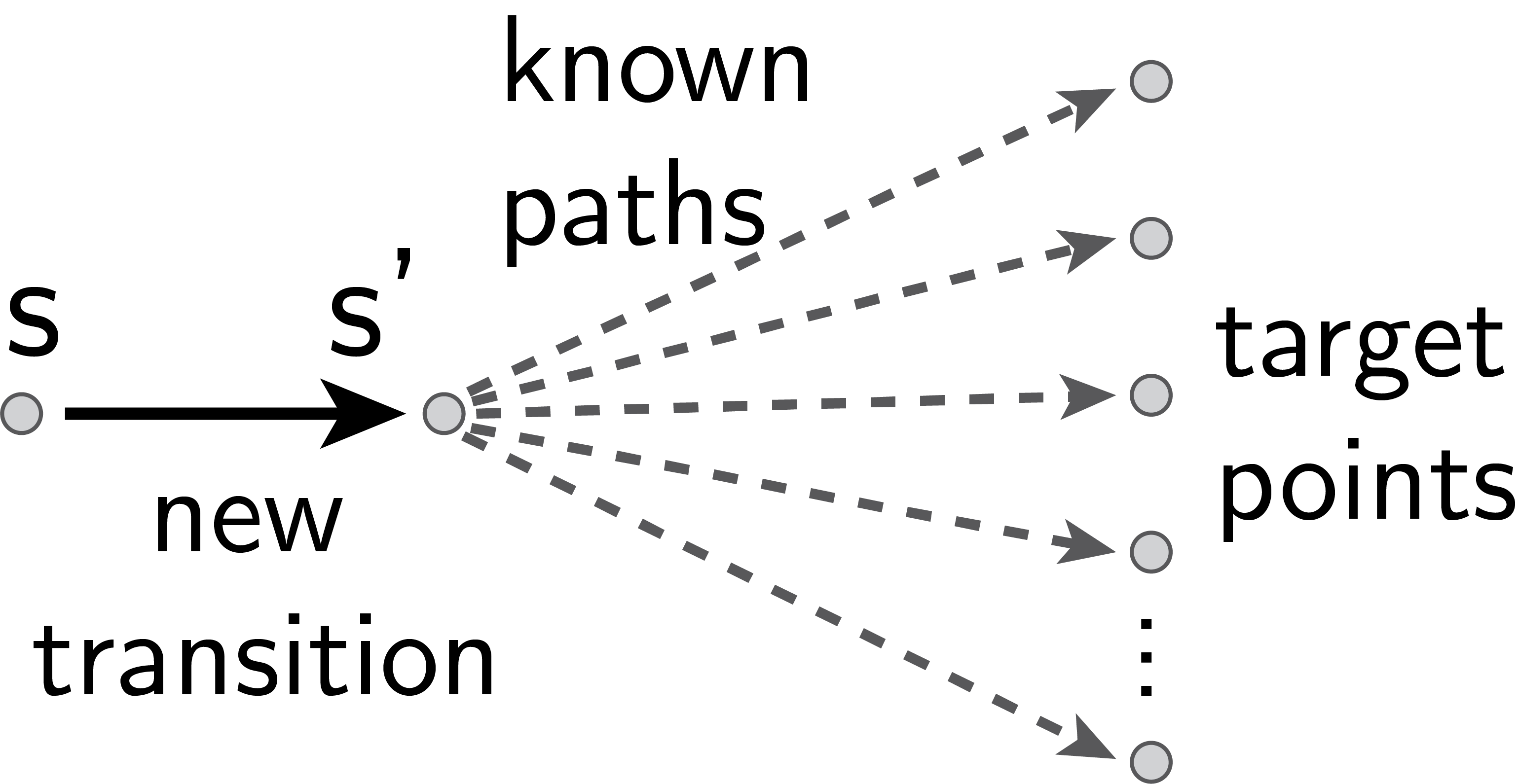
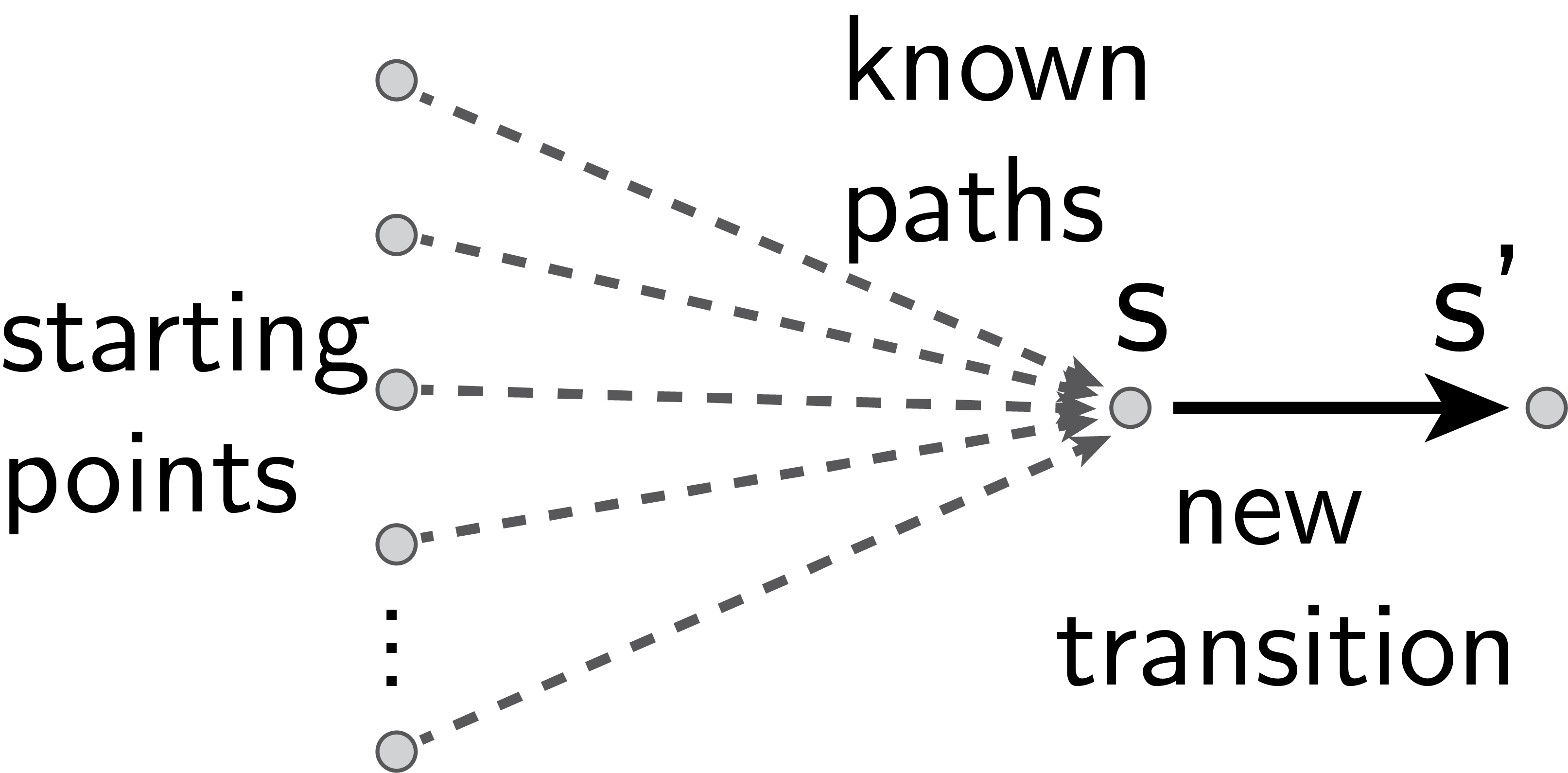
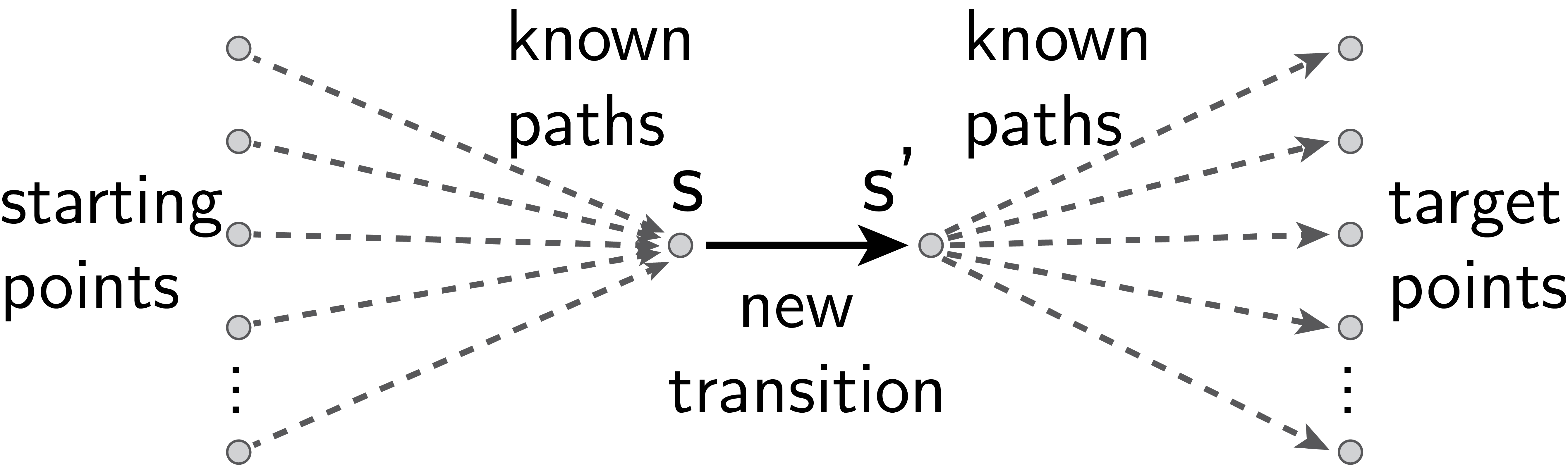
Figure 1: Combining paths: forward TD, backward TD, and path composition (Bellman–Newton).

The difference between forward and backward TD for $M$ is best understood in the path viewpoint on $M$ (Eq. 12). Indeed, the current estimate of $M_{s_{1}s_{2}}$ contains a current estimation on the number of paths from $s_{1}$ to $s_{2}$, weighted by their estimated probabilities in the Markov process. TD replaces $M$ with $PM$, and adds $\operatorname{Id}$, which represents the trivial paths from $s$ to $s$. Backward TD uses $MP$ instead. In both cases, the operator $P$ is sampled via an observed transition $s\to s^{\prime}$. Thus, $PM$ builds new known paths by taking all paths contained in $M$ and adding the transition $s\to s^{\prime}$ at the front of each path, while $MP$ adds the transition $s\to s^{\prime}$ at the back of each path in $M$ (Fig. 1). Forward TD reasons at fixed target states (rewards) (Greydanus and Olah, 2019), while backward TD reasons at fixed starting points.

Thus, TD and backward TD on $M$ differ in how they learn new paths from known paths when each new transition is observed. Arguably, both are reasonable ways to update a mental model of paths in an environment when discovering new transitions (e.g., if a new street $s\to s^{\prime}$ opens in a city).

There is a third way to build new paths when observing a new transition $s\to s^{\prime}$: take all known paths to $s$, all known paths from $s^{\prime}$, and insert $s\to s^{\prime}$ in the middle (Fig. 1). This exploits path concatenation, roughly doubling the length of known paths. This operation is involved in the way that $M$ actually changes when the process is changed by increasing $P(s,\operatorname{d}\!{}s^{\prime})$ (the way possible paths actually change when a new street opens). This is the basis of the “second-order” algorithms we present for $M$ in Section 7.

5 Multiple Policies: Goal-Dependent $Q$ and $V$ functions

The principles above can be used to learning goal-dependent policies and a goal-dependent value or $Q$ function, just by letting the policy be goal-dependent in the results above. This option only covers rewards located at a given target state, not dense rewards; it can also cover target features of states rather than a fully specified target state (Section 5.2), namely, having target values for some function $\varphi$ of the state. A first application is to learn all optimal policies to reach any goal state $s_{2}$, either via $Q$-learning (Section 5.1) or $V$-learning (Section 5.2).

This approach partially solves the well-known sparse reward problem in goal-dependent learning. For instance, let us consider the goal-dependent value function $V(s,\operatorname{d}\!{}s_{2})$: for every target state $s_{2}$, it solves the $s_{2}$-dependent Bellman equation

$$V(s,\operatorname{d}\!{}s_{2})=\delta_{s}(\operatorname{d}\!{}s_{2})+\gamma\mathbb{E}_{s^{\prime}\sim P(\operatorname{d}\!{}s^{\prime}|s,s_{2})}V(s^{\prime},\operatorname{d}\!{}s_{2})$$ (30)

with reward when $s=s_{2}$, and $s_{2}$-dependent policy $P(\operatorname{d}\!{}s^{\prime}|s,s_{2})$. (In the continuous case, the goal-dependent value function is a measure on $s_{2}$, because the probability to exactly reach a state is usually $0$. We will learn its density with respect to a reference measure.)

Using TD directly on this equation leads to sparse reward problems: in continuous state spaces, a reward is never observed (and rarely observed in large discrete spaces).

However, the contribution of the reward $\delta_{s}(\operatorname{d}\!{}s_{2})$ to the TD update can be computed exactly in expectation. The resulting update does not involve sparse rewards anymore: every transition is informative because it shows how to reach the currently visited state (as discussed in Section 4.1.3). This update is the same as with successor states: the update for $\tilde{m}$ in Theorem 6 can be directly used to train goal-dependent policies by seeing $\tilde{m}(s,s_{2})$ as the value function at $s$ when the goal state is $s_{2}$ (see the example after Theorem 13).

Existing workarounds for this sparse reward issue include strategies for resampling state-goal pairs that more frequently lead to nonzero rewards, such as Hindsight Experience Replay (HER) (Andrychowicz et al., 2017), which works with any $Q$-learning method, assuming knowledge of the reward function associated to each goal. It is not clear to us whether HER actually solves the infinitely-sparse-reward issue or not. The results described here are not mutually exclusive with using HER: HER is a sampling strategy for transitions in the training set, which can be used with any $Q$-learning method, such as those presented here; so in principle HER could be used as the state-goal distribution $\rho_{SG}$ for $Q$-learning in Theorem 13.

We start with learning the optimal $Q$ function for every target state (Section 5.1). We first describe the precise meaning of goal-dependent Bellman equations such as (30), and present the resulting parametric update.

Next we turn to a more general statement involving either the $V$ or $Q$ function, and target features instead of target states (Section 5.2). We discuss three use cases: $Q$-learning with any goal feature function, $V$-learning conditioned to goal states, and $V$-learning conditioned to goal features, which presents some subtleties. The goal-dependent $V$ function can be used to train goal-dependent policies by any policy gradient method.

In Section 5.3 we provide mathematical details for the existence and uniqueness of goal-dependent Bellman equations, in the case of the $Q$ function. Having to work with measures of potentially infinite mass results in non-uniqueness of the solution, but there is still a “natural” solution, equal both to the smallest solution and to the limit of the finite-horizon solution.

5.1 The Optimal $Q$-function for Every Goal State

Several works have attempted to learn optimal $Q$ functions indexed by an additional “goal” which encodes a variable reward. The simplest case is when the reward is located at a single goal state $g$. Computing the $Q$ function $Q(s,a,g)$ for every goal state $g$ fully solves the navigation problem in an environment, although this function does not provide the optimal policies for “mixed” rewards, only for single-state rewards.

The viewpoint presented here allows for a more principled approach to this object $Q$; notably, it can avoid the sparse reward problem of algorithms that sample a state $s$ and a goal state $g$ independently, with reward $\mathbbm{1}_{s=g}$. This is avoided thanks to the direct algebraic treatment of Diracs or sparse rewards discussed above.

So far, the successor state operator was defined for a given, fixed policy. The goal-dependent $Q$ function uses a different (optimal) policy for every goal. It can be defined through the optimal Bellman operator.

Definition 11 (Optimal Bellman operator for successor states).

Let $Q(s,a,\operatorname{d}\!{}s_{2})$ be a measure on $s_{2}$ depending on a state-action pair $(s,a)$. Define the optimal Bellman operator $T$ via

$$(TQ)(s,a,\operatorname{d}\!{}s_{2})\mathrel{\mathop{:}}=\delta_{s}(\operatorname{d}\!{}s_{2})+\gamma\,\mathbb{E}_{s^{\prime}\sim P(s^{\prime}|s,a)}\sup_{a^{\prime}}Q(s^{\prime},a^{\prime},\operatorname{d}\!{}s_{2}).$$ (31)

In the discrete case, this is just the usual optimal Bellman operator in parallel for every goal state $s_{2}$, namely, $(TQ)(s,a,s_{2})=\mathbbm{1}_{s=s_{2}}+\gamma\,\mathbb{E}_{s^{\prime}\sim P(s^{\prime}|s,a)}\max_{a^{\prime}}Q(s^{\prime},a^{\prime},s_{2})$. In the continuous case, for each state-action $(s,a)$, $Q(s,a,\cdot)$ is a measure over the state space, and the supremum $\sup_{a^{\prime}}Q(s^{\prime},a^{\prime},\operatorname{d}\!{}s_{2})$ is a supremum of measures over $s_{2}$.

In the discrete case, a fixed point exists by standard contractivity arguments; however, with continuous states, the situation is tricky, see Section 5.3. In particular, with continuous states the measure $Q$ may have either finite or infinite mass; intuitively, the total mass of $Q$ indicates how many distinct policies we can follow to reach different states. The total mass of $Q(s,a)$ is the total number of distinct points that can be reached from $(s,a)$ by taking different action sequences, weighted by the probability and discounted by time. In contrast, the successor state operator of a single fixed policy (Sections 3–4) always has total mass $\sum\gamma^{t}=\frac{1}{1-\gamma}$: there is no choice of actions so the total probability of states is $1$ at each time step.

To see this, consider two extreme examples. In the first, the environment just ignores every action and sends the agent to a random uniform state at each time step. Then for any $(s,a)$, $Q(s,a,\operatorname{d}\!{}s_{2})$ is $\delta_{s}(\operatorname{d}\!{}s_{2})+\frac{\gamma}{1-\gamma}\operatorname{d}\!{}s_{2}$, with total mass $\frac{1}{1-\gamma}$. In the second example, for every state we have an action that sends us directly to that state. Then $Q(s,a,\operatorname{d}\!{}s_{2})$ is a measure for which every single state $s_{2}\neq s$ has mass $\frac{\gamma}{1-\gamma}$, and the total mass of $Q(s,a,\cdot)$ is infinite. This can be arranged even with finite action spaces: generally, at horizon $t$ the mass may be as large as $\gamma^{t}(\#A)^{t}$ if every action sequence leads to a different part of the state (examples in Appendix B.4). In the fixed-policy case, the mass at horizon $t$ was always $\gamma^{t}$ and the total mass was always finite.

Parametric goal-dependent $Q$-learning.

Let us consider parametric models for $Q$. As before, we consider two models given by

$$Q_{\theta}(s,a,\operatorname{d}\!{}s_{2})\mathrel{\mathop{:}}=\delta_{s}(\operatorname{d}\!{}s_{2})+q_{\theta}(s,a,s_{2})\rho(\operatorname{d}\!{}s_{2})$$ (32)

and

$$Q_{\theta}(s,a,\operatorname{d}\!{}s_{2})\mathrel{\mathop{:}}=\tilde{q}_{\theta}(s,a,s_{2})\rho(\operatorname{d}\!{}s_{2})$$ (33)

respectively, and we will learn $q_{\theta}$ and $\tilde{q}_{\theta}$. For instance, up to the factor $\rho$, the models in (Schaul et al., 2015) correspond to $\tilde{q}_{\theta}(s,a,s_{2})=h(\varphi_{\theta}(s,a),\psi_{\theta}(s_{2}))$.

The resulting parametric update is as follows. The update is off-policy: we assume access to a dataset of transitions $(s,a,s^{\prime})$ in a Markov decision process. Let $\rho_{\mathrm{SA}}$ be the distribution of the state-action pair $(s,a)$ in the dataset; its marginal over $s$ is $\rho$ as before. Given a measure-valued function of $(s,a)$, such as $Q(s,a,\operatorname{d}\!{}s_{2})$, we define its norm similarly to (1) as

$$\left\lVert Q\right\rVert^{2}_{\rho_{\mathrm{SA}},\rho}\mathrel{\mathop{:}}=\mathbb{E}_{(s,a)\sim\rho_{\mathrm{SA}},\,s_{2}\sim\rho}[q(s,a,s_{2})^{2}]$$ (34)

where $q(s,a,s_{2})\mathrel{\mathop{:}}=Q(s,a,\operatorname{d}\!{}s_{2})/\rho(\operatorname{d}\!{}s_{2})$ is the density of $Q$ with respect to $\rho$, if it exists (otherwise the norm is infinite).

Theorem 12 (Parametric $Q$-learning for every goal state).

Consider a parametric model of $Q$ given by (32) or (33), where $q_{\theta}(s,a,s_{2})$ or $\tilde{q}(s,a,s_{2})$ are smooth functions depending on the parameter $\theta$.

Let $\theta_{0}$ be some value of the parameter. Define a target update $Q^{\mathrm{tar}}$ of $Q$ via the optimal Bellman operator (31) applied to $Q_{\theta_{0}}$, namely, $Q^{\mathrm{tar}}(s,a,\operatorname{d}\!{}s_{2})\mathrel{\mathop{:}}=(TQ_{\theta_{0}})(s,a,\operatorname{d}\!{}s_{2})=\delta_{s}(\operatorname{d}\!{}s_{2})+\gamma\,\mathbb{E}_{s^{\prime}\sim P(s^{\prime}|s,a)}\sup_{a^{\prime}}Q_{\theta_{0}}(s^{\prime},a^{\prime},\operatorname{d}\!{}s_{2})$. Define the loss between $Q_{\theta}$ and $Q^{\mathrm{tar}}$ via $J(\theta)\mathrel{\mathop{:}}=\frac{1}{2}\left\lVert Q_{\theta}-Q^{\mathrm{tar}}\right\rVert^{2}_{\rho_{\mathrm{SA}},\rho}$ using the norm (34).

Then the gradient step on $\theta$ to reduce this loss is

$$-\partial_{\theta}J(\theta)=\mathbb{E}_{(s,a)\sim\rho_{\mathrm{SA}},\,s^{\prime}\sim P(s^{\prime}|s,a),\,s_{2}\sim\rho}\left[\gamma\,\partial_{\theta}q_{\theta}(s,a,s^{\prime})\right.\\ \left.+\,\partial_{\theta}q_{\theta}(s,a,s_{2})\left(\gamma\sup_{a^{\prime}}q_{\theta_{0}}(s^{\prime},a^{\prime},s_{2})-q_{\theta}(s,a,s_{2})\right)\right]$$ (35)

for the model (32) using $q_{\theta}$, and

$$-\partial_{\theta}J(\theta)=\mathbb{E}_{(s,a)\sim\rho_{\mathrm{SA}},\,s^{\prime}\sim P(s^{\prime}|s,a),\,s_{2}\sim\rho}\left[\partial_{\theta}\tilde{q}_{\theta}(s,a,s)\right.\\ \left.+\,\partial_{\theta}\tilde{q}_{\theta}(s,a,s_{2})\left(\gamma\sup_{a^{\prime}}\tilde{q}_{\theta_{0}}(s^{\prime},a^{\prime},s_{2})-\tilde{q}_{\theta}(s,a,s_{2})\right)\right]$$ (36)

for the model (33) using $\tilde{q}_{\theta}$.

Here we have presented the update using a fixed “target network” with parameter $\theta_{0}$ (typically a previous value of $\theta$), a common practice for parametric $Q$-learning.

This update is “samplable”: sample a transition $(s,a,s^{\prime})$ from the dataset, another independent transition $(s_{2},a_{2},s^{\prime}_{2})$ from the dataset ($a_{2}$ and $s^{\prime}_{2}$ are discarded), and estimate the gradient by

$$\widehat{\operatorname{\delta}{}\theta}=\gamma\,\partial_{\theta}q_{\theta}(s,a,s^{\prime})+\partial_{\theta}q_{\theta}(s,a,s_{2})\left(\gamma\sup_{a^{\prime}}q_{\theta_{0}}(s^{\prime},a^{\prime},s_{2})-q_{\theta}(s,a,s_{2})\right)$$ (37)

or likewise for $\tilde{q}$ (only the first term is different).

This update is perfectly analogous to the successor state updates for $m_{\theta}$ and $\tilde{m}_{\theta}$ in Theorem 6, except that $q_{\theta}$ and $\tilde{q}_{\theta}$ depend on the actions, and that the policy follows a supremum over actions instead of being fixed.

As before, the infinite, infinitely sparse rewards $\delta_{s}(\operatorname{d}\!{}s_{2})$ of the every-goal problem produce the finite contribution $\gamma\,\partial_{\theta}q_{\theta}(s,a,s^{\prime})$ or $\partial_{\theta}\tilde{q}(s,a,s)$ in this parametric update. Sampling two independent states $s$ and $s_{2}$ is still needed, but for the Bellman gap term, not for the reward term.

5.2 Value and $Q$ Functions with State Features as Goals

We now turn to a general result covering both value and $Q$ functions ($Q$ functions are obtained as the value function of the state-action Markov process, as explained in Section 2). We also cover target features rather than target states: namely, we are given a feature function $\varphi$ on state space, and the reward is nonzero on states $s$ such that $\varphi(s)$ achieves a particular goal value $g$. Target states correspond to $\varphi=\operatorname{Id}$.

Covering $V$ functions requires the ability to work on-policy. Thus, we assume that goal-dependent policies are given, yielding goal-dependent transitions $s\to s^{\prime}|g$ defined by their transition probabilities $P(\operatorname{d}\!{}s^{\prime}|s,g)$.

Thus we wish to find solutions to the goal-dependent Bellman equation

$$V(s,\operatorname{d}\!{}g)=\delta_{\varphi(s)}(\operatorname{d}\!{}g)+\gamma\,\mathbb{E}_{s^{\prime}\sim P(\operatorname{d}\!{}s^{\prime}|s,g)}V(s^{\prime},\operatorname{d}\!{}g)$$ (38)

with reward on states such that the features $\varphi(s)$ are equal to $g$. Full target states amount to $\varphi=\operatorname{Id}$: a nonzero reward when $s=g$. This can be used in turn to train the goal-dependent policies, for instance by policy gradient. (The technical meaning of this equation is similar to the case of $Q$ above. For a discussion on existence and uniqueness we refer to Section 5.3.)

Here the training dataset is made of triplets $(s\to s^{\prime}|g)$: transitions indexed by a goal. For the $Q$ function this is not restrictive: working on state-action pairs, given a state-action $(s,a,s^{\prime})$ it is always possible to sample a goal $g$ a posteriori, and to define the next action $a^{\prime}$ according to policy $g$ in state $s^{\prime}$. For the $V$ function this is more restrictive: typically, the training set would be made of trajectories where a goal is selected at random and kept for some time. This results in some empirical distribution over state-goal pairs $(s,g)$ in the training set, with $s$ and $g$ not independent.

A major issue is to avoid using the sparse rewards $\delta_{\varphi(s)}(\operatorname{d}\!{}g)$. Indeed, the most obvious approach to the Bellman equation (38) is to view this problem as an ordinary Markov process on the augmented state space of state-goal pairs $(s,g)$. The TD update for this problem is

$$\operatorname{\delta}{}\theta =\mathbb{E}_{(s,g)\sim\rho_{SG},\,s^{\prime}\sim P(\operatorname{d}\!{}s^{\prime}|s,g)}\left[\partial_{\theta}v_{\theta}(s,g)\left(\frac{\delta_{s}(\operatorname{d}\!{}g)}{\tau(\operatorname{d}\!{}g)}+\gamma v_{\theta}(s^{\prime},g)-v_{\theta}(s,g)\right)\right]$$

where $\rho_{SG}$ is the distribution of state-goal pairs $(s,g)$ in the training set, and where the $V$ function has been parameterized as $V_{\theta}(s,\operatorname{d}\!{}g)=v_{\theta}(s,g)\tau(\operatorname{d}\!{}g)$ for some arbitrary measure $\tau(\operatorname{d}\!{}g)$ on goal space. In a continuous state space, no reward would ever be observed.

Sparse rewards can be avoided by just using the goal $g=\varphi(s)$ for the sparse term: $\partial_{\theta}v_{\theta}(s,g)\,\delta_{s}(\operatorname{d}\!{}g)\leadsto\partial_{\theta}v_{\theta}(s,\varphi(s))$. The price to pay is computing the value function only up to a goal-dependent scaling. Namely, there is a simple sparsity-free TD update for the related problem

$$V(s,\operatorname{d}\!{}g)=\alpha(s,g)\,\delta_{\varphi(s)}(\operatorname{d}\!{}g)+\gamma\,\mathbb{E}_{s^{\prime}\sim P(\operatorname{d}\!{}s^{\prime}|s,g)}V(s^{\prime},\operatorname{d}\!{}g).$$ (39)

Here the reward is nonzero only if $\varphi(s)=g$, but with an unknown factor $\alpha(s,g)$ that depends on the solution reached.

If $\alpha(s,g)$ depends only on $g$, then optimal policies are not affected: for every goal $g$, we just compute the correct value function for this goal up to a $g$-dependent scaling. This happens in many use cases, notably for $Q$-learning or if $\varphi=\operatorname{Id}$ (goals are full states), as shown below.

The least favorable use case is $V$-learning with $\varphi\neq\operatorname{Id}$. Then the scaling $\alpha$ may also vary among the states $s$ which achieve $\varphi(s)=g$: this may result in policies which do solve the problem of finding a state $s$ with $\varphi(s)=g$, but not necessarily in an optimal way. (In that case, another option is to explicitly provide a full state $s_{g}$ such that $\varphi(s_{g})=g$ and use the full state $s_{g}$ as the goal instead, thus going back to $\varphi=\operatorname{Id}$.)

We now turn to the technical, general statement and discuss some explicit use cases. The theorem is stated for $V$ functions; the case of $Q$ functions follows by applying it to the state-action Markov process.

Theorem 13 (Goal-dependent TD).

Let $\varphi\colon S\to\mathcal{G}$ be a function from the state space to some goal space $\mathcal{G}$ (discrete if $S$ is discrete and continuous if $S$ is continuous).

Assume that the training set consists of transitions $(s\to s^{\prime}|g)$ indexed by a goal. Let the joint distribution of state-goal pairs in the training set be $\rho_{SG}(\operatorname{d}\!{}s,\operatorname{d}\!{}g)$. Let $\rho_{S}$ and $\rho_{G}$ be its marginals over $s$ and $g$, namely, the distributions of states and of goals in the training set. Assume that the density of $\rho_{SG}$ with respect to $\rho_{S}\rho_{G}$ is nonzero everywhere (every state-goal pair appears with some positive probability).

Parameterize the value function as $V_{\theta}(s,\operatorname{d}\!{}g)=v_{\theta}(s,g)\rho_{G}(\operatorname{d}\!{}g)$.

Then the parameter update

$$\operatorname{\delta}{}\theta =\mathbb{E}_{(s,g)\sim\rho_{SG},\,s^{\prime}\sim P(\operatorname{d}\!{}s^{\prime}|s,g)}\left[\,\partial_{\theta}v_{\theta}(s,\varphi(s))+\partial_{\theta}v_{\theta}(s,g)\left(\gamma v_{\theta}(s^{\prime},g)-v_{\theta}(s,g)\right)\right]$$ (40)

is the TD update associated with the Bellman equation for the goal-dependent value function

$$V(s,\operatorname{d}\!{}g)=\alpha(s,g)\,\delta_{\varphi(s)}(\operatorname{d}\!{}g)+\gamma\,\mathbb{E}_{s^{\prime}\sim P(\operatorname{d}\!{}s^{\prime}|s,g)}V(s^{\prime},\operatorname{d}\!{}g).$$ (41)

where $\alpha(s,g)\mathrel{\mathop{:}}=\rho_{S}(\operatorname{d}\!{}s)\rho_{G}(\operatorname{d}\!{}g)/\rho_{SG}(\operatorname{d}\!{}s,\operatorname{d}\!{}g)$. (Note that the value of $\alpha(s,g)$ is used only on states such that $\varphi(s)=g$.)

In the following cases, $\alpha$ depends only on $g$:

• If the distributions of states and goals are independent in the training set, namely, if $\rho_{SG}(s,g)=\rho_{S}(s)\rho_{G}(g)$, then $\alpha(s,g)=1$.

• If $\varphi=\operatorname{Id}$ (goals are full states) then the statement also holds with $\alpha(g,g)$ instead of $\alpha(s,g)$ in (41).

Concretely, a stochastic update $\operatorname{\delta}{}\theta$ is obtained by sampling from the dataset a transition $(s\to s^{\prime}|g)$ indexed by a goal $g$, and then updating by

$$\operatorname{\delta}{}\theta=\partial_{\theta}v_{\theta}(s,\varphi(s))+\partial_{\theta}v_{\theta}(s,g)\left(\gamma v_{\theta}(s^{\prime},g)-v_{\theta}(s,g)\right).$$ (42)

This is similar to the update of $\tilde{m}_{\theta}$ in successor states (Theorem 6), except here the policy depends on the goal. This can be used in turn to train a goal-depedent policy (Section 8).

This theorem can work out in three different ways:

• $Q$-learning works for any goal features $\varphi$, using an ordinary off-policy training set of transitions $((s,a)\to s^{\prime})$. In that case, there is no need for transitions to be indexed by a goal. This follows from the theorem applied to the state-action process, and yields $\alpha=1$.

• $V$-learning works best with full goal states ($\varphi=\operatorname{Id}$). This requires a training set of transitions $(s\to s^{\prime}|g)$ each indexed by a goal state (such as exploring with a given goal for some time). A goal-dependent policy can be trained by any policy gradient method. In that case, $\alpha$ depends only on $g$, thus, computing the value function for every $g$ up to a $g$-dependent scaling that does not affect the optimal policy for $g$.

• $V$-learning can be applied with any goal features $\varphi$, but the resulting algorithm implicitly reweights the rewards among those states which achieve a given goal. Goal-dependent policies training by policy gradient will still reach a state such that $\varphi(s)=g$, but not necessarily in an optimal way, with certain states implicitly preferred.

Let us discuss the first two cases in more detail.

With $Q$-learning, it is possible to pick any goal a posteriori for any observed transition $((s,a)\to s^{\prime})$. So goals and states can be picked independently, resulting in $\alpha=1$. This plays out as follows: Assume the training set is made of transitions $((s,a)\to s^{\prime})$, that we have a set of goals $g\in\mathcal{G}$, and that we maintain the value function $v_{\theta}((s,a),g)$ over state-action pairs. Assume we have $g$-dependent policies $\pi_{g}$, such as the greedy policy obtained from the $Q$-function $v_{\theta}((s,a),g)$. Then the expected TD update (40) can be realized by picking at random a transition $((s,a)\to s^{\prime})$ in the dataset, picking at random a goal $g\sim\rho_{G}(\operatorname{d}\!{}g)$ according to any user-chosen distribution on goals, picking an action $a^{\prime}\sim\pi_{g}(s^{\prime})$, and updating the parameter via

$$\operatorname{\delta}{}\theta=\partial_{\theta}v_{\theta}((s,a),\varphi(s,a))+\partial_{\theta}v_{\theta}((s,a),g)\left(\gamma v_{\theta}((s^{\prime},a^{\prime}),g)-v_{\theta}((s,a),g)\right).$$ (43)

With $V$-learning, it is unreasonable to assume that goals and states are independent in the training set: this would require an exploration policy which randomly changes goals at every step. A more reasonable exploration policy would pick a goal $g\sim\rho_{G}$ and keep it for some time, using the goal-dependent policy $\pi_{g}$. This results in a set of transitions $(s\to s^{\prime}|g)$ indexed by their goals, with a non-independent distribution of goals and visited states, thus $\alpha\neq 1$. If $\varphi=\operatorname{Id}$ the theorem states that $\alpha$ only depends on $g$ so that optimal policies are not affected. The expected TD update (40) can be realized by picking at random a transition $(s\to s^{\prime}|g)$ in the dataset and updating the parameter via

$$\operatorname{\delta}{}\theta=\partial_{\theta}v_{\theta}(s,s)+\partial_{\theta}v_{\theta}(s,g)\left(\gamma v_{\theta}(s^{\prime},g)-v_{\theta}(s,g)\right).$$ (44)

This update of $v_{\theta}$ is identical to the update of $\tilde{m}_{\theta}$ in successor states (Theorem 6), except here the transitions (or policy) depends on the goal.

There is no variance from sparse rewards in these expressions: the reward term produces the term $\partial_{\theta}v_{\theta}(s,\varphi(s))$, namely, a term directly evaluated at the goal $g=\varphi(s)$ associated with the currently visited state $s$. (But there is still some variance from the Bellman gap part of the expression.) Thus, when learning goal-dependent value or $Q$ functions with sparse rewards, it is possible to avoid the sparse reward problem by directly setting the goal $g=\varphi(s)$ for the reward term in the TD update.

For comparison, algorithms such as hindsight experience replay store a mixture of state-related and state-independent goals in a training dataset of transitions, to be used with any off-policy learning algorithm. As in our setting, they assume knowledge of the reward function (such as $\delta_{\varphi(s)}(\operatorname{d}\!{}g)$) and access to a way to build goals from states, such as $\varphi$. This provides a strategy for building a relevant state-goal distribution in the training set. Such an approach is independent from our results, which directly reduce the variance in the $Q$-learning update. Thus in principle both approaches can be used simultaneously.

Multi-step, horizon-$k$ versions of TD (Appendix A.2) do not seem to be available in the goal-dependent setting in a version that avoids the infinitely-sparse Dirac reward problem.

5.3 Existence and Uniqueness of Optimal Successor States

We now turn to finding a solution to the optimal goal-dependent Bellman equation $TQ=Q$.

For discrete, infinite Markov reward processes, the value function that solves the Bellman equation is in general not unique; it is unique under additional constraints such as boundedness.

For the optimal goal-dependent $Q$-function, we cannot impose boundedness, since the solution sometimes has infinite mass. Instead, we prove that the solution for the horizon-$t$ problem exists and converges to the smallest solution of the Bellman equation when $t\to\infty$.

Let $Q_{t}$ be the goal-dependent $Q$-function at bounded horizon $t$, obtained by expanding the expectimax problem at horizon $t$, namely

$$Q_{t}(s_{1},a_{1},\operatorname{d}\!{}s_{g})\mathrel{\mathop{:}}=\delta_{s_{1}}(\operatorname{d}\!{}s_{g})\,+\\ \mathbb{E}_{s_{2}\sim P(s_{2}|s_{1},a_{1})}\sup_{a_{2}}\left[\gamma\delta_{s_{2}}(\operatorname{d}\!{}s_{g})+\cdots\mathbb{E}_{s_{t}\sim P(s_{t}|s_{t-1},a_{t-1})}\sup_{a_{t}}\left[\gamma^{t}\delta_{s_{t}}(\operatorname{d}\!{}s_{g})\right]\cdots\right].$$ (45)

This $Q_{t}$ can also be described via the optimal Bellman operator $T$ as $Q_{t}=T^{t}\mathbf{0}$, with $\mathbf{0}$ the zero measure. (In the following, “$Q$ is a measure” is short for “for every state-action $(s,a)$, $Q(s,a,\cdot)$ is a measure”.)

Theorem 14.

Let $T$ be the optimal Bellman operator of Definition 11. Let $\mathbf{0}$ be the measure with mass $0$.

Let $Q_{t}\mathrel{\mathop{:}}=T^{t}\mathbf{0}$ be the goal-dependent $Q$-function at horizon $t$. Then when $t\to\infty$, $Q_{t}$ converges strongly to a measure $Q^{\ast}$. This limit solves the Bellman equation $TQ^{\ast}=Q^{\ast}$, and is the smallest such solution. In finite state spaces, it is the only solution with finite mass.

The solution is never unique: the measure that gives infinite mass to every set is another. Hence the interest of considering the smallest solution, where the values come from rewards actually picked at some time $t$.

6 Matrix Factorization and the Forward-Backward (FB) Representation

6.1 Advantages of Matrix Factorization for $M$

In this section we study a specific parametric model for the successor state operator, which has many advantages: a “matrix-factorized” representation. We consider the model (15), namely $M(s_{1},\operatorname{d}\!{}s_{2})\approx\tilde{m}_{\theta}(s_{1},s_{2})\rho(\operatorname{d}\!{}s_{2})$, with the particular choice

$$\tilde{m}_{\theta}(s_{1},s_{2})=F_{\theta_{F}}(s_{1})^{\!\top}\!B_{{\theta_{B}}}(s_{2})$$ (46)

where $F\colon S\to{\mathbb{R}}^{r}$ and $B\colon S\to{\mathbb{R}}^{r}$ are two learnable functions from the state space to some representation space ${\mathbb{R}}^{r}$, parameterized by $\theta=({\theta_{F}},{\theta_{B}})$. This provides an approximation of $M$ by a rank-$r$ operator. Such a factorization is used for instance in (Schaul et al., 2015) for the goal-dependent $Q$-function (up to the factor $\rho$).

Intuitively, $F$ is a “forward” representation of states and $B$ a “backward” representation: if the future of $s_{1}$ matches the past of $s_{2}$, then $M(s_{1},\operatorname{d}\!{}s_{2})$ is large. The learning algorithms presented above (forward and backward TD for $M$) can be directly applied to this parameterization, leading to explicit updates for $F$ and $B$ (Section 6.2).

This representation of $M$ has a number of advantages and some shortcomings. (In this section we deal mostly with successor states; for goal-dependent value functions, this representation has fewer advantages.) The advantages are as follows.

• It provides a direct representation of the value function at every state, without learning an additional model of $V$. Namely,

  $$V(s)\approx F(s)^{\!\top}\!B(R),\qquad B(R)\mathrel{\mathop{:}}=\mathbb{E}_{s\sim\rho}[r_{s}\,B(s)]$$ (47)

  where the “reward representation” $B(R)$ can be directly estimated by an online average of $B(s)$ weighted by the reward $r_{s}$ at $s$. This is a direct consequence of (17). For instance, with sparse rewards, each time a reward is observed, the value function is updated everywhere.

  This point applies to successor states, but not to goal-dependent value functions, which cannot handle arbitrary rewards.

• It simplifies the sampling of a pair of states $(s,s_{2})$ needed for forward TD. Indeed, the forward TD update (21) factorizes as an expectation over $s$, times an expectation over $s_{2}$ (Section 6.2 below), which can be estimated independently. The same applies to backward TD. This can potentially reduce variance a lot, and even allows for purely “trajectory-wise” online estimates using only the current transition $s\to s^{\prime}$, without sampling of another independent state $s_{2}$. (Once more, this works for successor states but not for goal-dependent value functions, since in that case the transitions $s\to s^{\prime}$ depend on $s_{2}$.)

• It produces two (policy-dependent) representations of states, a forward and a backward one, in a natural way from the dynamics of the MDP and the current policy. This could be useful for other purposes.

• Even in the tabular case, when the state space is discrete and unstructured, this provides a form of prior or generalization between states (based on a low-rank prior for the successor state operator). States that are linked by the MDP dynamics get representations $F$ and $B$ that are close.

• It has some of the properties of the second-order methods of Section 7, without their complexity. This is proved in Appendix F.1.

The shortcomings are as follows:

• It approximates the successor state operator by an operator of rank at most $r$. This is never an exact representation unless the representation dimension $r$ is at least the number of distinct states.

• The best rank-$r$ approximation of $(\operatorname{Id}-\gamma P)^{-1}$ erases the small singular values of $P$: thus this representation will tend to erase “high frequencies” in the reward and value function, and provide a spatially smoother approximation focusing on long-range behavior. This is fine as long as the reward is not a “fast-changing” function made up of high frequencies (such as a “checkerboard” reward).

  This can be expected: learning a reward-agnostic object such as $M$ cannot work equally well for all rewards. For these reasons, it may be useful to use a mixed model for the value function with the FB model as a baseline, such as

  $$V_{\varphi}(s)=F(s)^{\!\top}\!B(R)+v_{\varphi}(s)$$ (48)

  where $F$ and $B$ are learned via successor states, $B(R)$ is as in (47), and $\varphi$ is learned via ordinary TD on the remainder. The $FB$ part will catch reward-independent, long-range behavior, while the $v_{\varphi}$ part will be needed to catch high frequencies in a particular reward function.

Why is a matrix-factorized form relevant for $M$?

Small-rank approximations of a matrix are relevant when the matrix has a few large eigenvalues and many small eigenvalues (or singular values, depending on the precise criterion). Since the successor state operator is the inverse of $\operatorname{Id}-\gamma P$, this means the approximation is reasonable if $\operatorname{Id}-\gamma P$ has few small eigenvalues and many large eigenvalues.

The spectrum of Markov operators is a well-studied topic. For continuous-time operators associated with random diffusions, possibly with added drift, the spectrum generally follows Weyl’s law (Wikipedia, 2021): in dimension $d$, the continuous-time analogue of $\operatorname{Id}-P$ has roughly $k^{d/2}$ eigenvalues of size $\leqslant k$, thus, few small and many large eigenvalues.

The simplest example is a random walk on a discrete torus $[1;n]$. The operator $P$ is diagonal in Fourier representation, with eigenvectors $e^{2i\pi kx/n}$ with $k$ an integer. The corresponding eigenvalue of $P$ is $\cos(2\pi k/n)$, yielding an eigenvalue $(1-\gamma)+2\gamma\sin^{2}(\pi k/n)$ for $\operatorname{Id}-\gamma P$. The largest eigenvalue of $P$ is $1$ (for $k=0$) corresponding to the smallest eigenvalue $1-\gamma$ for $\operatorname{Id}-\gamma P$. For $\gamma$ close to $1$, $(\operatorname{Id}-\gamma P)^{-1}$ has a very large eigenvalue $1/(1-\gamma)$, then an eigenvalue of order $n^{2}/2\pi^{2}$, and the next eigenvalues behave like $n^{2}/2k^{2}\pi^{2}$, thus decreasing like $1/k^{2}$. In this case, a small-rank approximation is reasonable. A similar computation holds for periodic grids $[1;n]^{d}$ in higher dimension.

How general is this example? The best studied case is for continuous-time diffusions in continuous spaces such as a subset in ${\mathbb{R}}^{d}$. In continuous time, the analogue of the operator $\operatorname{Id}-\gamma P$ is the infinitesimal generator operator of the continuous-time Markov process. For the standard Brownian motion, this operator is the Laplacian $\Delta=\sum_{i=1}^{d}\partial^{2}/\partial x_{i}^{2}$. Its inverse $\Delta^{-1}$ plays the role of the successor state operator and provides the value function in continuous time. The spectrum of the Laplacian is well-known and follows Weyl’s law: there are about $k^{d/2}$ eigenvalues of size $\leqslant k$ (Wikipedia, 2021). In particular, $\Delta$ has few small eigenvalues and many large eigenvalues, so that the successor state operator (given by $\Delta^{-1}$, which provides the value function in continuous time) has few large eigenvalues and many small eigenvalues as needed.

This applies not only to Brownian motion, but to basically any diffusion with drift and variable coefficients on a subset of ${\mathbb{R}}^{d}$: indeed, in this case the infinitesimal generator is an elliptic operator and also follows Weyl’s law (Gårding, 1953). The same law also holds for diffusions on Riemannian manifolds, as the Riemannian Laplace operator also follows Weyl’s law (Berger, 2003, Chapter 9.7.2). These continuous estimates are still valid when discretizing the state space (Xu et al., 2017). So this situation is quite general.

6.2 The TD Updates for the FB Representation of $M$

We now describe the explicit parametric TD updates for the FB representation of successor states. These follow directly from the general expressions for forward TD and backward TD.

However, the particular factorized structure gives rise to more variants: pure forward (forward TD on $F$ and $B$), forward-backward (forward TD update for $F$ but backward TD update for $B$), etc. These will lead to slightly different fixed points and different dynamics for feature learning, as we will explore later.

Proposition 15 (Successor state TD updates in the FB representation).

Consider the parameterization $\tilde{m}_{\theta}(s_{1},s_{2})=F_{\theta_{F}}(s_{1})^{\!\top}\!B_{{\theta_{B}}}(s_{2})$ of the successor state operator $M$ where $F$ and $B$ are two functions from $S$ to ${\mathbb{R}}^{r}$, parameterized by $\theta=({\theta_{F}},{\theta_{B}})$. Abbreviate $F$ for $F_{\theta_{F}}$ and $B$ for $B_{\theta_{B}}$.

Then the forward TD update (21) for $F$ is equal to

$$\mathbb{E}_{s\sim\rho}\,(\partial_{{\theta_{F}}}F(s)^{\!\top}\!)B(s)+\mathbb{E}_{s\sim\rho,s^{\prime}\sim P(s,\operatorname{d}\!{}s^{\prime})}\,(\partial_{{\theta_{F}}}F(s)^{\!\top}\!)\,\Sigma_{B}(\gamma F(s^{\prime})-F(s))$$ (49)

where $\Sigma_{B}$ is the matrix

$$\Sigma_{B}\mathrel{\mathop{:}}=\mathbb{E}_{s_{2}\sim\rho}\,B(s_{2})B(s_{2})^{\!\top}\!.$$ (50)

The forward TD update for $B$ is equal to

$$\mathbb{E}_{s\sim\rho}\,(\partial_{\theta_{B}}B(s)^{\!\top}\!)F(s)+\mathbb{E}_{s_{2}\sim\rho}\,(\partial_{\theta_{B}}B(s_{2})^{\!\top}\!)\,D_{F}B(s_{2}).$$ (51)

where $D_{F}$ is the matrix

$$D_{F}\mathrel{\mathop{:}}=\mathbb{E}_{s\sim\rho,\,s^{\prime}\sim P(s,\operatorname{d}\!{}s^{\prime})}\,F(s)(\gamma F(s^{\prime})-F(s))^{\!\top}\!.$$ (52)

The backward TD update for $F$ is equal to

$$\mathbb{E}_{s\sim\rho}\,(\partial_{\theta_{F}}F(s)^{\!\top}\!)B(s)+\mathbb{E}_{s_{1}\sim\rho}\,(\partial_{\theta_{F}}F(s_{1})^{\!\top}\!)\,D_{B}F(s_{1}),$$ (53)

where $D_{B}$ is the matrix

$$D_{B}\mathrel{\mathop{:}}=\mathbb{E}_{s\sim\rho,\,s^{\prime}\sim P(s,\operatorname{d}\!{}s^{\prime})}(\gamma B(s^{\prime})-B(s))B(s)^{\!\top}\!.$$ (54)

The backward TD update for $B$ is equal to

$$\mathbb{E}_{s\sim\rho}\,(\partial_{\theta_{B}}B(s)^{\!\top}\!)F(s)+\mathbb{E}_{s\sim\rho,\,s^{\prime}\sim P(s,\operatorname{d}\!{}s^{\prime})}\left(\gamma\,\partial_{\theta_{B}}B(s^{\prime})^{\!\top}\!-\partial_{\theta_{B}}B(s)^{\!\top}\!\right)\Sigma_{F}B(s)$$ (55)

where $\Sigma_{F}$ is the matrix

$$\Sigma_{F}\mathrel{\mathop{:}}=\mathbb{E}_{s_{1}\sim\rho}\,F(s_{1})F(s_{1})^{\!\top}\!.$$ (56)

Proposition 34 (Appendix E) describes how these updates play out for finite spaces in the “tabular on FB” setting, in which a value of $F$ and $B$ is maintained for each state.

Forward or backward TD may be used separately for $F$ and $B$, giving rise to four algorithms: forward on $F$ and forward on $B$ (ff-FB), forward on $F$ and backward on $B$ (fb-FB), backward on $F$ and forward on $B$ (bf-FB), and backward on $F$ and backward on $B$ (bb-FB). These algorithms behave quite differently on how they learn features and on the fixed points obtained, as discussed below.

Consequences for sampling and variance.

A key feature of the FB updates is their decomposition as a product of an expectation over a transition $s\to s^{\prime}$, times an expectation over another independent state $s_{2}$ or $s_{1}$.

This has important consequences algorithmically for variance reduction via minibatching. Indeed, a natural way to sample these updates would be to sample a minibatch of transitions $s\to s^{\prime}$, another minibatch of states $s_{2}$, and evaluate (49) on the minibatch $s\to s^{\prime}$ with the value of $\Sigma_{B}$ obtained on the minibatch $s_{2}$. This would not be possible for other parameterizations of $M$: in general, (21) would require to compute a separate quantity for each $(s\to s^{\prime},s_{2})$, thus requiring smaller minibatches in practice.

Furthermore, these updates lend themselves to a purely trajectory-wise online estimation, without even sampling another independent state $s_{2}$ or $s_{1}$: indeed, (49) can be estimated at the current transition $s\to s^{\prime}$, while the matrices $\Sigma_{F}$ etc., may be estimated online by an exponential moving average over past or recent states.

Fixed points, feature learning.

With $F$ and $B$ of dimension $r$, each of the $r$ components of $F$ and $B$ defines a function $F_{i}(s)$ or $B_{i}(s)$ on the state space. We call these functions features. The features of $F$ provide a basis for approximating the value function $V$. In addition, the model for $V$ ignores any part of the reward function that is uncorrelated to the features of $B$.

More precisely, the kernel of $B$ and the image of $F^{\!\top}\!$ directly encode which features of states are ignored. Namely, if $R\in\operatorname{Ker}B\rho$ then the corresponding value function is estimated to $0$: $MR=F^{\!\top}\!B\rho R=0$. Thus $\operatorname{Ker}B\rho$ encodes the subspace of reward functions that is unseen by the model. $\operatorname{Ker}B\rho$ is exactly the space of functions which are $L^{2}(\rho)$-orthogonal to all the features in $B$. Likewise, for any reward function $R$, the approximate value function is $F^{\!\top}\!B\rho R=0$ which lies inside $\operatorname{Im}F^{\!\top}\!$: thus $\operatorname{Im}F^{\!\top}\!$ is the space of features used to express the value functions.

The four algorithms ff-FB, fb-FB, bf-FB, and bb-FB greatly differ on how new features are learned:

• ff-FB learns new features by applying the operator $P$ to existing features in $F$. These new features are put into both $F$ and $B$. The fixed points of ff-FB correspond to eigenvectors of the matrix $P$ and $M$ (Proposition 36).

• bb-FB learns new features by applying the operator $P^{\!\top}\!$ to existing features in $B$, and putting them into both $F$ and $B$. The fixed points of bb-FB correspond to eigen-probability densities of $P$ and $M$ (Remark 38, Proposition 37).

• fb-FB learns new features both by applying $P$ to features in $F$, and $P^{\!\top}\!$ to features in $B$. The fixed points of fb-FB are the rank-$r$ truncated SVD decompositions of the matrix $M$.

• bf-FB may not learn any features beyond the initialization of $F$ and $B$. For any subspace of features, there is a fixed point of bf-FB which lies in that subspace.

We refer to Appendix E for precise statements of these properties. In addition, fb-FB and bf-FB preserve the symmetry with respect to time reversal of the process, while ff-FB and bb-FB do not.

Relationship with successor representation learning and with linear TD with learned features.

To help interpreting these relations, we will relate them to objects from the literature. We make two claims. First, for fixed and orthonormal $B$, the forward update of $F$ corresponds to standard successor representation learning with state representation (features) $B$. Second, for fixed $F$, the forward update of $B$ corresponds to learning the value function for every target state via linear TD with fixed features $F$.

To simplify things, in this paragraph we consider the “tabular-FB” setting, in which $F$ and $B$ are parameterized just by listing the value of $F(s)$ and $B(s)$ on every state $s$, assuming a finite state space. For instance, the forward TD update (49) for $F$, with learning rate $\eta>0$, becomes $F(s)\leftarrow F(s)+\eta\operatorname{\delta}{}F(s)$ where

$$\operatorname{\delta}{}F(s)=B(s)+\Sigma_{B}(\gamma F(s^{\prime})-F(s))$$ (57)

upon sampling a transition $s\to s^{\prime}$.

If $B$ is a fixed, $L^{2}(\rho)$-orthonormal collection of feature functions (namely, if $\Sigma_{B}=\operatorname{Id}$), then this forward TD equation to learn $F$ is identical to standard deep successor representation learning using $B$ as the representation. Indeed, standard deep successor representation learning (Kulkarni et al., 2016) starts with given features $\varphi(s)$ on the state space, and learns the successor features $m$ as the expected discounted future value of $\varphi$ along a trajectory $(s_{t})$: $m(s)=\sum_{t\geqslant 0}\gamma^{t}\mathbb{E}[\varphi(s_{t})|s_{0}=s]$. Such an $m$ is the fixed point of the Bellman equation $m=\varphi+\gamma Pm$. Via identifying $m=F$ and $\varphi=B$, ordinary TD for this Bellman equation is equivalent to (57) when $\Sigma_{B}=\operatorname{Id}$. However, this is not the case if $\Sigma_{B}\neq\operatorname{Id}$. This is because scalings are different: With the successor state operator, if $B$ is doubled, then $F$ is halved so that $M=F^{\!\top}\!B$ is fixed. With successor representations, if the state representation $\varphi$ is doubled, then $m$ is doubled as well.

Next, if $F$ is fixed, we claim that the forward TD update for $B$ corresponds to linear TD to learn all value functions corresponding to individual reward $\mathbbm{1}_{s_{2}}$ at all target states $s_{2}$, with $F$ as the feature basis. Indeed, if the reward function is $R=\mathbbm{1}_{s_{2}}$, and the corresponding value function is represented as $V=F^{\!\top}\!w$ for some learned vector $w$ (this is linear TD with feature basis $F$), then the TD update of $w$ when observing a transition $s\to s^{\prime}$ is $\operatorname{\delta}{}w=F(s)\left(\mathbbm{1}_{s=s_{2}}+\gamma F(s^{\prime})^{\!\top}\!w-F(s)^{\!\top}\!w\right).$ Of course, the resulting $w$ depends on $s_{2}$. Thus, if we learn a vector $w(s_{2})$ this way for every $s_{2}$, we get an update $\operatorname{\delta}{}w(s_{2})=F(s)\left(\mathbbm{1}_{s=s_{2}}+\gamma F(s^{\prime})^{\!\top}\!w(s_{2})-F(s)^{\!\top}\!w(s_{2})\right)$. By identifying $w(s_{2})$ and $B(s_{2})$, then on expectation over $s$ and $s_{2}$ sampled from $\rho$, this is equal to (51) for tabular $B$. Thus, for fixed $F$, the forward TD update (51) just puts into every $B(s_{2})$ a representation of the value function for reward $\mathbbm{1}_{s_{2}}$ as a linear combination of the features $F(s)$.

Thus, when learning $F$ and $B$ jointly, the “FB-tabular” forward TD update on $F$ and $B$ can be seen as a simultaneous learning of all value functions for all reward $\mathbbm{1}_{s_{2}}$, by linear TD in a learned feature basis $F$.

7 Second-Order Methods for Successor States: Implicit Process Estimation and Bellman–Newton

We now turn to more complex, “second-order” algorithms for estimating successor states and value functions. First, we study the best online estimate of $M$ and $V$ in the tabular case, obtained by directly estimating the transition matrix and reward function, and exactly solving the Bellman equation in this estimated process. We provide a convergence theorem for this method (Theorem 16).

This provides an explicit online evolution equation for $M$ and $V$ from observed transitions, in which the transition matrix does not appear (successor states via implicit process estimation, Theorem 17). Interestingly, this “true” update of $V$ is TD preconditioned by $M$ (Theorem 18). This is related to viewing $M_{s_{1}s}$ as an expectation of the eligibility trace at state $s$ (Appendix D).

The resulting “true” update of $M$, taken in expectation, defines a Bellman–Newton operator (Definition 19), so called because it corresponds exactly to the Newton method for inverting the matrix $M$. Intuitively, this operator proceeds by concatenating known paths of the MDP, thus doubling the length of known paths, while TD and backward TD just add one transition to the set of known paths (see intuition in Section 4.3). This intuition is formalized in several ways (Proposition 20, Appendix C). This also translates as much better asymptotic convergence in the continuous-time limit (Section 9.3).

All these properties are exact analogues of the convergence properties of second-order Newton-like methods compared to simple first-order gradient descent. Thus, online estimation of $M$ and the Bellman–Newton operator can be seen as “second-order” TD algorithms. Accordingly, they are also numerically trickier. Strengths and weaknesses are discussed in Section 7.4.

Finally, we derive the parametric version of the Bellman–Newton operator, extending it beyond full-matrix tabular updates to sampling in arbitrary state spaces. However, this update has a large variance unless some kind of forward-backward (FB) representation is used.

7.1 Estimating a Markov Process Online

We now introduce estimates of $M$ and $V$ by online estimation of the Markov process, first in the tabular case, then via function approximation. The process estimation is implicit: it does not appear in the resulting algorithms for $M$. (In particular, we never store an estimated transition matrix $\hat{P}$, which would not make sense for continuous spaces; this excludes solving the problem by planning via the model $\hat{P}$.)

In a (small) finite state space, an obvious approach to learn $M$ is to first learn an estimate $(\hat{P},\hat{R})$ of the transition matrix $P$ and reward vector $R$ of the Markov reward process, by direct empirical averages; then set $M$ and $V$ to their true values in the estimated Markov process, namely, $\hat{M}=\sum_{n\geqslant 0}\gamma^{n}\hat{P}^{n}=(\operatorname{Id}-\gamma\hat{P})^{-1}$ and $\hat{V}=\hat{M}\hat{R}$.

The empirical averages $\hat{P}$ and $\hat{R}$ are updated for each new transition $s\to s^{\prime}$ with reward $r_{s}$, by updating the row $s$ of the transition matrix $\hat{P}$, and the value $\hat{R}_{s}$ at $s$:

$$\hat{P}_{ss_{2}} \leftarrow(1-1/n_{s})\hat{P}_{ss_{2}}+(1/n_{s})\mathbbm{1}_{s_{2}=s^{\prime}}\quad\forall s_{2},\qquad\hat{R}_{s}\leftarrow(1-1/n_{s})\hat{R}_{s}+(1/n_{s})r_{s}$$ (58)

with $n_{s}$ the number of visits to state $s$ up to time $t$. The initialization of $\hat{P}$ and $\hat{R}$ is forgotten after the first observation at each state ($n_{s}=1$), but to fix ideas we initialize to $\hat{P}=\hat{R}=0$. The corresponding estimates $\hat{M}=(\operatorname{Id}-\gamma\hat{P})^{-1}$ and $\hat{V}=\hat{M}\hat{R}$ converge to their true values, as shown by the following non-asymptotic bound.

Theorem 16 (Convergence bounds for process estimation).

Consider a finite Markov reward process with $S$ states and $E$ edges ($(s,s^{\prime})$ is an edge if $P_{ss^{\prime}}>0$), rewards almost surely bounded by $R_{\mathrm{max}}$, and stationary distribution $\rho$. Update $\hat{P}$ and $\hat{R}$ online via (58), initialized to $\hat{P}=\hat{R}=0$.

Then after $t$ i.i.d. observations $(s\mathbin{\sim}\rho,\,s^{\prime}\mathbin{\sim}P_{ss^{\prime}})$, with probability $1-\delta$, the estimates $\hat{M}=(\operatorname{Id}-\gamma\hat{P})^{-1}$ and $\hat{V}=\hat{M}\hat{R}$ satisfy

$$\|\hat{M}-M\|_{\rho,\mathrm{TV}}\leqslant\frac{2\gamma}{(1-\gamma)^{2}}\sqrt{\frac{2E}{t}\log\frac{2}{\delta}}$$ (59)

and

$$\sum_{s}\rho(s)\left\lvert\hat{V}(s)-V(s)\right\rvert\leqslant\frac{3R_{\mathrm{max}}}{(1-\gamma)^{2}}\sqrt{\frac{2E}{t}\log\frac{4S}{\delta}}.$$ (60)

These bounds do not depend on the sampling measure $\rho$, although the norm used to define the error does. Thus, rarely visited points have no impact on these bounds.

Direct matrix inversion is inconvenient. But since (58) is a rank-one update of the matrix $\hat{P}$, one can compute the update of $\hat{M}$ resulting from (58); this update does not explicitly involve $\hat{P}$ anymore. This will form the basis for the parametric version.

We call the resulting algorithm successor states via implicit process estimation (SSIPE).

Theorem 17 (SSIPE: Tabular online update of $M$).

When a transition $s\to s^{\prime}$ is added to an empirical estimate of a Markov reward process via (58), the successor state matrix $\hat{M}$ of the estimated process becomes $\hat{M}\leftarrow\hat{M}+\operatorname{\delta}{}M$ with

$$\operatorname{\delta}{}M_{s_{1}s_{2}}=\frac{1}{n_{s}}\,\hat{M}_{s_{1}s}\,\frac{\mathbbm{1}_{s_{2}=s}+\gamma\hat{M}_{s^{\prime}s_{2}}-\hat{M}_{ss_{2}}}{1-\frac{1}{n_{s}}(\gamma\hat{M}_{s^{\prime}s}-\hat{M}_{ss}+1)} \qquad\forall s_{1},s_{2}$$ (61)

with $n_{s}$ the number of times state $s$ has been sampled. The estimated value function $\hat{V}$ becomes $\hat{V}\leftarrow\hat{V}+\operatorname{\delta}{}V$ with

$$\operatorname{\delta}{}V_{s_{1}}=\tfrac{1}{n_{s}}(r_{s}+\gamma\hat{V}_{s^{\prime}}-\hat{V}_{s})\,\hat{M}_{s_{1}s}+o(1/n_{s}) \qquad\forall s_{1}$$ (62)

where $r_{s}$ is the observed reward.

This describes the “true” change of $M$ when the Markov process changes by increasing $P_{ss^{\prime}}$. This update contains a two-sided term $M_{s_{1}s}M_{s^{\prime}s_{2}}$: in terms of paths, this term combines all known paths from $s_{1}$ to $s$, the transition $s\to s^{\prime}$, then all known paths from $s^{\prime}$ to $s_{2}$ (Fig. 1 and Appendix C).

The update of $V$ has the form $\delta V=M\cdot(\text{Bellman gap at }$s$)$. The matrix $M$ can be seen as a “credit assignment” to transfer the Bellman gap $R+\gamma PV-V$ observed at a state $s$ to “predecessor” states.

The update (61) of $M$ is also its TD update multiplied on the left by $M$ (compare (61) and (19)). This is most clear when taking expectations over the next transition $s\to s^{\prime}$, as follows.

Theorem 18 (The true change of $M$ and $V$ is TD preconditioned by $M$).

Estimate the successor matrix and value function of a finite MRP by $\hat{M}=(\operatorname{Id}-\gamma\hat{P})^{-1}$ and $\hat{V}=\hat{M}\hat{R}$ where $\hat{P}$ and $\hat{R}$ are estimated directly by the empirical averages (58).

Consider the updates of these estimates after observing a new transition $s\to s^{\prime}$. Then, in expectation over the transition $s\to s^{\prime}$ sampled at time $t$, the update (61) of $\hat{M}$ is equal to

$$\mathbb{E}_{s\mathbin{\sim}\rho,\,s^{\prime}\mathbin{\sim}P_{ss^{\prime}}}[\operatorname{\delta}{}M]=\tfrac{1}{t}\hat{M}(\operatorname{Id}+\gamma P\hat{M}-\hat{M})+o(1/t)$$ (63)

when the number of observations $t$ tends to infinity. The resulting update of the value function is $\hat{V}\leftarrow\hat{V}+\operatorname{\delta}{}V$ with

$$\mathbb{E}_{s\mathbin{\sim}\rho,\,s^{\prime}\mathbin{\sim}P_{ss^{\prime}}}[\operatorname{\delta}{}V]=\tfrac{1}{t}\hat{M}(R+\gamma P\hat{V}-\hat{V})+o(1/t).$$ (64)

Thus, preconditioning the TD update by $M$ itself produces an update that tracks the “true” value of $M$ and $V$ given all observations available so far. The learning rate $1/t$ is inherited from the direct estimate of $P$ and $R$ via empirical averages in (58).

This update of $V$ is consistent with the view of $M$ as an expected eligibility trace (Appendix D). Indeed, eligibility traces also update the value function at states $s_{1}$ that are connected to $s$ via a trajectory. Actually, in expectation, these updates are the same: with $\lambda=1$, the eligibility trace vector at a state $s$ is an unbiased estimator of the column $M_{s_{1}s}$ (Theorem 31 in Appendix D). From this viewpoint, learning $M$ via a parametric model, or using TD($1$), are both ways of estimating the “predecessor states” of a state $s$. Eligibility traces are unbiased but can have large variance, while the model of $M$ has no variance but may have bias if not learned well.

Such a preconditioning is analogous to second-order methods in optimization using the inverse Hessian, which directly jump to the the location of the new optimum when one more data point becomes available. However, in second-order methods, the preconditioning matrix is symmetric definite positive, while this is not the case here; this can produce numerical problems.

In small-scale experiments, using the full matrix online update of $\hat{M}$ resulted in much faster convergence of the value function than TD, consistently with the theoretical prediction of Section 9.3. But with this method, each update requires $O(\left\lvert S\right\rvert^{2})$ computation time. This is useful only if sample efficiency is the main concern.

7.2 The Bellman–Newton Operator

Thus, when estimating a Markov process online, in expectation, each new observation replaces the estimate $\hat{M}$ with $\hat{M}+\mathbb{E}[\operatorname{\delta}{}M]=\hat{M}(1+\frac{1}{t})-\frac{1}{t}\hat{M}(\operatorname{Id}-\gamma P)\hat{M}+o(1/t)$ by (63). Interestingly, this expected update does not depend on the distribution $\rho$ of sampled states $s$. This is because the $1/n_{s}$ factors behave asymptotically like $1/(t\rho_{s})$, thus compensating the sampling probabilities $\rho_{s}$. The fluctuations between $n_{s}$ and $t\rho_{s}$ are absorbed in the $o(1/t)$ terms. We gather this behavior in the following operator.

Definition 19 (Bellman–Newton operator).

We call Bellman–Newton operator with learning rate $\eta>0$ the operator $M\mapsto M(1+\eta)-\eta M(\operatorname{Id}-\gamma P)M$.

The reason for the name is the following: With learning rate $\eta=1$, this operator is $M\mapsto 2M-M(\operatorname{Id}-\gamma P)M$. Inverting a matrix $A$ by iterating $M\leftarrow 2M-MAM$ is the Newton method for matrix inversion, going as far back as 1933 (Pan and Schreiber, 1991). The Newton method has superexponential convergence, squaring the error (doubling precision) at each step. This property translates as follows in our context.

In terms of paths, the quadratic term in $M$ realizes the path concatenation operation in Fig. 1. This is formalized as follows, and proved and further discussed in Appendix C. In contrast, forward and backward TD only increase the length of known paths by $1$.

Proposition 20 (Bellman–Newton doubles the length of known paths).

Assumes that $M$ represents exactly the successor states up to $k$ steps, namely, $M=\sum_{i=0}^{k}\gamma^{i}P^{i}$ (as matrices or as operators). Then after one step of the Bellman–Newton operator with learning rate $\eta=1$, $M$ represents exactly the successor states up to $2k+1$ steps, namely, $2M-M(\operatorname{Id}-\gamma P)M=\sum_{i=0}^{2k+1}\gamma^{i}P^{i}$.

Unfortunately, this method does not always converge. In particular, it is initialization-dependent. For instance, the initialization $M=0$ is a fixed point. In general, the Bellman–Newton operator preserves the kernel and image of $M$, so there are many fixed points. Still, $M=(\operatorname{Id}-\gamma P)^{-1}$ is the only full-rank fixed point.

Convergence of the Newton method for matrix inversion is quite well understood (Pan and Schreiber, 1991) and works if the spectral radius of $\operatorname{Id}-AM$ is less than $1$ at initialization. Otherwise, the method can diverge. For instance, $A=\operatorname{Id}-\gamma P$ for successor states, so initializing to $M=\operatorname{Id}$ converges.

Learning rates $\eta\ll 1$ improve convergence properties. In Section 9.3 we study convergence with infinitesimal learning rates, proving much faster asymptotic convergence than with simple TD on $M$. This is analogous to the faster convergence of second-order methods with respect to simple gradient descent. Even with $\eta\ll 1$, some initializations still diverge; however, if the initialization is of the form $M=(\operatorname{Id}-\gamma P_{0})^{-1}$ for some stochastic or substochastic matrix $P_{0}$ (e.g., $P_{0}=0$, initializing $M$ to $\operatorname{Id}$) then the infinitesimal learning rate version converges.

Sampled Bellman–Newton update.

Like the Bellman operator for TD on $M$, the Bellman–Newton operator lends itself to sampling the states at which the values are updated.

This works out as follows. Assume that $S$ is discrete so that $M$ is a matrix (we deal with the parametric case in the next section). Let as usual $\rho$ be the probability distribution from which states are sampled, and let $\grave{\rho}$ be the matrix with diagonal entries $\rho$. Set $\tilde{m}\mathrel{\mathop{:}}=M\grave{\rho}^{-1}$ (this corresponds to the parameterization $\tilde{m}$ in (15)). Then the Bellman–Newton update is equivalent to $\tilde{m}\mapsto\tilde{m}(1+\varepsilon)-\eta\tilde{m}(\grave{\rho}-\gamma\grave{\rho}P)\tilde{m}$. In expectation, this update can be realized by sampling a state $s\sim\rho$ and a transition $s^{\prime}\sim P(\operatorname{d}\!{}s^{\prime}|s)$. Indeed, in that case we have $\mathbb{E}\mathbbm{1}_{s}\mathbbm{1}^{\!\top}\!_{s^{\prime}}=\grave{\rho}P$ and $\mathbb{E}\mathbbm{1}_{s}\mathbbm{1}^{\!\top}\!_{s}=\grave{\rho}$, and therefore the update

$$\tilde{m}_{s_{1}s_{2}}\leftarrow(1+\eta)\tilde{m}_{s_{1}s_{2}}-\eta\,\tilde{m}_{s_{1}s}\,\tilde{m}_{ss_{2}}+\eta\,\gamma\,\tilde{m}_{s_{1}s}\,\tilde{m}_{s^{\prime}s_{2}}\qquad\forall s_{1},s_{2}$$ (65)

is equal to the Bellman–Newton update in expectation over $(s,s^{\prime})$.

This is still a full-matrix update: the value $\tilde{m}_{s_{1}s_{2}}$ is updated for every $s_{1}$ and $s_{2}$, even if $(s,s^{\prime})$ is sampled. This is not scalable. It is possible to sample the states $s_{1}$ and $s_{2}$ from $\rho$ as well: with this option, the expectation of the update is multiplied by $\grave{\rho}$ on the left and right.

7.3 Parametric Bellman–Newton Update

Perhaps surprisingly, the full-matrix tabular update of $M$ lends itself well to a parametric version, by following the standard TD strategy of updating the parameter to bring $M$ closer to its new value.

Theorem 21 (Bellman–Newton update with function approximation).

Maintain a parametric model of $M$ via $m_{\theta_{t}}$ or $\tilde{m}_{\theta_{t}}$ as in Section 3.2, with $\theta_{t}$ the parameter at step $t$.

Let $s\to s^{\prime}$ be the transition in the Markov process observed at step $t$, with reward $r_{s}$. Define a target update of $M$ by $M^{\mathrm{tar}}\mathrel{\mathop{:}}=M_{\theta_{t}}+\operatorname{\delta}{}M$ with $\operatorname{\delta}{}M$ given by the online tabular estimate (61). Define the loss between $M$ and $M^{\mathrm{tar}}$ via $J(\theta)\mathrel{\mathop{:}}=\frac{1}{2}\left\lVert M_{\theta}-M^{\mathrm{tar}}\right\rVert_{\rho}^{2}$ using the norm (1).

Then the gradient step on $\theta$ to reduce this loss is

$$-\partial_{\theta}J(\theta)_{|\theta=\theta_{t}}={\textstyle\frac{1}{t}}\,\mathbb{E}_{s_{1}\sim\rho,\,s_{2}\sim\rho}\left[\gamma\,\partial_{\theta}m_{\theta_{t}}(s,s^{\prime})+\gamma\,m_{\theta_{t}}(s_{1},s)\,\partial_{\theta}m_{\theta_{t}}(s_{1},s^{\prime})\right.\\ +\left.(\gamma m_{\theta_{t}}(s^{\prime},s_{2})-m_{\theta_{t}}(s,s_{2}))\left(\partial_{\theta}m_{\theta_{t}}(s,s_{2})+m_{\theta_{t}}(s_{1},s)\,\partial_{\theta}m_{\theta_{t}}(s_{1},s_{2})\right)\right]+o(1/t)$$ (66)

for the model (16) using $m_{\theta}$, and

$$-\partial_{\theta}J(\theta)_{|\theta=\theta_{t}}={\textstyle\frac{1}{t}}\,\mathbb{E}_{s_{1}\sim\rho,\,s_{2}\sim\rho}\left[\tilde{m}_{\theta_{t}}(s_{1},s)\,\partial_{\theta}\tilde{m}_{\theta_{t}}(s_{1},s)\right.\\ +\left.\tilde{m}_{\theta_{t}}(s_{1},s)(\gamma\tilde{m}_{\theta_{t}}(s^{\prime},s_{2})-\tilde{m}_{\theta_{t}}(s,s_{2}))\,\partial_{\theta}\tilde{m}_{\theta_{t}}(s_{1},s_{2})\right]+o(1/t)$$ (67)

for the model (15) using $\tilde{m}_{\theta}$.

The update of $V$ via $M$ is discussed in Section 8.

Here the learning rate $1/t$ is inherited from the direct estimate of $P$ via empirical averages, but can be replaced with any learning rate. As with TD, the update was derived from a tabular update, but makes sense in continuous state spaces. In particular, the parametric gradient does not involve the state counts $n_{s}$ from (61): a cancellation occurs because $n_{s}\sim t\rho_{s}$ when $t\to\infty$.

Implementing this update requires sampling two additional states $s_{1}$ and $s_{2}$ from the dataset, in addition to the transition $s\to s^{\prime}$. See the discussion after Theorem 6 for possible ways to sample these additional states. TD for $M$ required only one: this reflects the full matrix update (61), while TD only updates the $s$ row of $M$ when observing a new transition $s\to s^{\prime}$ (Eq. 19).

For parametric Bellman–Newton, the model $m_{\theta}$ can be initialized to $0$ while the model $\tilde{m}_{\theta}$ cannot. Indeed, setting $m_{\theta}$ to $0$ corresponds to setting $M$ to $\operatorname{Id}$, a valid initialization for the Bellman–Newton operator, while setting $\tilde{m}_{\theta}$ to $0$ corresponds to setting $M$ to $0$, an unwanted and unstable fixed point of the Bellman–Newton operator.

7.4 Discussion: strengths and weaknesses of second-order approaches

In a tabular setting, the full-matrix online update (61) of $M$ (where a transition $s\to s^{\prime}$ is sampled, but with the value $M_{s_{1}s_{2}}$ updated for every state $s_{1}$ and $s_{2}$) converges much faster than TD to compute the value function, empirically. This is in line with the asymptotic convergence properties of the Bellman–Newton versus ordinary Bellman operator (Section 9.3).

However, this results in an $O(\left\lvert S\right\rvert^{2})$ cost per time step, so it is only interesting if sample efficiency is the main issue. The alternative is to sample a few states $s_{1}$ and $s_{2}$ and only update $M_{s_{1}s_{2}}$ for those states. But in practice, we have found that this introduces many instabilities and requires reducing the learning rate so much (typically $\eta$ smaller than $1/\left\lvert S\right\rvert^{2}$) that the benefit of second-order Newton convergence is lost. The same phenomenon is observed for the parametric version of Theorem 21.

This sampling issue can be avoided if using a factorized representation $M=F^{\!\top}\!B$ as in Section 6. Namely, there exists an update of $F$ and $B$ that is compatible with sampling and that reproduces the Bellman–Newton update (Section F.2). This decouples the sampling of states $s_{1}$ and $s_{2}$, thus reducing variance and allowing for larger learning rates. However, this also exacerbates another issue of the Bellman–Newton update, namely, the existence of non-full-rank fixed points and the preservation of the kernel and image of $M$. The representation $M=F^{\!\top}\!B$ is usually not full-rank, and the Bellman–Newton update of Section F.2 preserves the kernels of $F$ and $B$. As a consequence (at least for uniform $\rho$), this algorithm computes the inverse of $\operatorname{Id}-\gamma P$ in the subspace spanned by the initializations of $F$ and $B$, but no features are learned. Currently, we have found no fully satisfactory second-order update beyond the full-matrix update (61).

8 Learning Value Functions and Policies via Successor States

There are many possible ways to use a model $M$ of the successor state operator in policy and and value function learning. Choices include:

• Using policy gradient versus using $Q$-learning (greedy or Boltzmann policies, DDPG…).

  If the reward is a known goal state, we may directly use the optimal goal-dependent $Q$ function of Section 5.1.

  For $Q$-learning with other types of rewards, the successor state operator can be defined on the Markov process over state-action pairs (as explained in Section 2). The $Q$ function can be computed from this “successor state-action operator” in the same ways as the $V$ function from the successor state operator. Thus, all methods described below to learn $V$ can be extended to $Q$, and we do not discuss this option further here.

• Using the goal-dependent value function as in Section 5 (this leads to a goal-dependent policy for every goal state, simultaneously for all single-state reward functions), versus using the successor state operator of a single policy as in Section 4 (this works for dense rewards but with a single policy).

• Using the successor state operator directly in the policy gradient formula without a value function model, versus learning a model of $V$ from successor states, then using this model normally in policy gradient.

• If learning a model of $V$ from successor states, there are several options to do so. First, the FB representation of $M$ directly yields a $V$ function. Second, the $V$ function may be learned from $M$ in a supervised way based on $V=MR$. Third, $M$ may be used only as one component of the value function ($V=MR+v_{\varphi}$ with $v_{\varphi}$ learned via TD), or as an initialization. This is presumably better if $M$ is approximate. Fourth, $V$ may be learned via TD “preconditioned by $M$”, based on the formula (64) for the true change of $V$ when new transitions are observed (Theorem 18).

We now describe these options in greater detail. They have different bias-variance trade-offs, and the best option may differ based form case to case.

We recall the general form of the policy gradient estimator for a parametric policy $\pi$

$$\operatorname{\delta}{}\pi\mathrel{\mathop{:}}=\mathbb{E}_{s\sim\rho}\mathbb{E}_{a\sim\pi(a|s)}\left[(\partial\ln\pi(a|s))\,\mathbb{E}_{s^{\prime}\sim P(\operatorname{d}\!{}s^{\prime}|s,a)}\left[r_{s,a}+\gamma V(s^{\prime})-b(s)\right]\right]$$ (68)

where $\partial\ln\pi(a|s)$ is the derivative with respect to the policy parameters of the log-probability to select action $a$, where $r_{s,a}$ is the immediate reward received after action $a$, and where $b$ is an arbitrary baseline function which reduces variance of the estimator (typically $b(s)=V(s)$ so that $r_{s,a}+\gamma V(s^{\prime})-b(s)$ is centered, but we will see other choices below).

Learning goal-dependent policies.

The simplest case is for learning policies to reach arbitrary target states, using the goal-dependent value function $v_{\theta}(s,g)$ of Section 5.2. Here $g$ represents a variable goal, such as a target state, or a desired value for some function of states (Section 5.2).

This works with a goal-dependent policy $\pi(a|s,g)$ depending on goal $g$, and leads to the policy gradient update

$$\operatorname{\delta}{}\pi=\mathbb{E}_{(s,g)\sim\rho_{SG},\,a\sim\pi(a|s,g),s^{\prime}|P(\operatorname{d}\!{}s^{\prime}|s,a)}(\partial\ln\pi(a|s,g))(\gamma v_{\theta}(s^{\prime},g)-b(s,g))$$ (69)

where $v_{\theta}$ is the goal-dependent value function model from Section 5.2, where $b$ is an arbitrary baseline function (such as $b(s,g)=v_{\theta}(s,g)$), and where $\rho_{SG}$ is the empirical distribution of state-goal pairs in the trajectories in the dataset (typically obtained by choosing a goal and following the associated policy for some time).

A few comments on this formula: First, with goal states, the reward $r_{s,a}$ in (68) is a Dirac mass, but it depends only on the previous state, not on $a$ or $s^{\prime}$; so by choosing the baseline $b$ to include this Dirac, this term disappears in (69).

Second, in the formalism of Section 5.2, the value function is formally a measure over goals, $V_{\theta}(s,\operatorname{d}\!{}g)=v_{\theta}(s,\operatorname{d}\!{}g)\rho_{G}(\operatorname{d}\!{}g)$. Thus, the policy gradient update (68) is goal-dependent and is itself a measure over goals $g$. This measure can be integrated over all goals $g$; for each $g$ we may choose the distribution $s\sim\rho_{SG}(\operatorname{d}\!{}s|g)$ of states given this goal. This is how we obtain the policy update (69) from (68). In the computation, the measures cancel out between $\rho_{SG}(\operatorname{d}\!{}s|g)$ and the $\rho_{G}(\operatorname{d}\!{}g)$ appearing in $V_{\theta}$: this results in just $v_{\theta}$ in (69), and in the sampling of a pair $(s,g)$ from $\rho_{SG(s,g)}$.

Learning $V$ from $M$.

Another option is to learn the value function $V$ using $M$, then just use the value function via ordinary policy gradient. We now consider the case of a single (non-goal-dependent) policy to be learned, with an arbitrary reward function. There are several options again.

• The FB representation of Section 6 directly provides a representation of the value function as

  $$V(s)\approx F(s)^{\!\top}\!B(R),\qquad B(R)\mathrel{\mathop{:}}=\mathbb{E}_{s\sim\rho}[r_{s}\,B(s)]$$ (70)

  where $B(R)$ is a “representation of the reward”, which can be sampled by weighting the representation $B(s)$ of states by their reward. Thus $B(R)$ can be estimated online. Then the value of $V$ can be plugged directly in the policy gradient formula (68).

  Since the FB representation will focus on low frequencies (long-range) features, it might be useful to used a “mixed” model for $V$, with $F(s)^{\!\top}\!B(R)$ as one component, and another component learned via ordinary TD; see (75) below.

• Another case is if the reward is located at a single known target state $g$. Then $V(s)=\tilde{m}(s,g)$ and the policy gradient (68) is equal to

  $$\operatorname{\delta}{}\pi=\mathbb{E}_{s\sim\rho}\mathbb{E}_{a\sim\pi(a|s)}\left[(\partial\ln\pi(a|s))\,\mathbb{E}_{s^{\prime}\sim P(\operatorname{d}\!{}s^{\prime}|s,a)}\left[\gamma\tilde{m}(s^{\prime},g)-b(s)\right]\right]$$ (71)

  (once more, the reward term $r_{s,a}$ does not depend on $a$ in that case and can be absorbed in the baseline $b$). This assumes the model $\tilde{m}$ is used for $M$; the model $m$ does not seem to lead to a usable formula in this case.

  This is useful for sparse rewards: contrary to TD methods, $M$ and $V$ may be learned without ever seeing the reward, provided the target state is known. (By “known”, we mean we know the features or input representation of the target state, as provided to the neural networks that learn $M$ and $V$.) This also extends to linear combinations of a finite number of rewards at known states.

• For general (dense) rewards and without the FB representation, the simplest option is to learn a model of $V$ based on $V=MR$. This becomes a supervised learning problem. No matrix product is necessary: we can perform a stochastic gradient descent of $\left\lVert V-MR\right\rVert^{2}_{L^{2}(\rho)}$ with respect to the parameters of $V$, just by sampling states, either with discrete or continuous states.

  With $V$ parameterized as $V_{\varphi}$, and with $M$ parameterized by the model $\tilde{m}_{\theta}$, we have

  $$-\partial_{\varphi}\left\lVert V_{\varphi}-MR\right\rVert^{2}_{L^{2}(\rho)}=2\mathbb{E}_{s\sim\rho,\,s_{1}\sim\rho}\left[\partial_{\varphi}V_{\varphi}(s_{1})(r_{s}\,\tilde{m}(s_{1},s)-V_{\varphi}(s_{1}))\right]$$ (72)

  where $r_{s}$ is the reward obtained when visiting state $s$. As for other algorithms presented here, this requires sampling one or several additional states $s_{1}$ in addition to the state $s$ currently visited.

  With $M$ parameterized by the model $m_{\theta}$ instead, we have

  $$-\partial_{\varphi}\left\lVert V_{\varphi}-MR\right\rVert^{2}_{L^{2}(\rho)}=\\ 2\mathbb{E}_{s\sim\rho,\,s_{1}\sim\rho}\left[\,r_{s}\,\partial_{\varphi}V_{\varphi}(s)+(r_{s}\,m(s_{1},s)-V_{\varphi}(s_{1}))\,\partial_{\varphi}V_{\varphi}(s_{1})\right].$$ (73)

• Learning $V$ via $V=MR$ assumes that the model of $M$ is reasonably accurate: any error on $M$ shows up on $V$. Another option is to just use $MR$ as a component in the model of $V$, or as an initialization to $V$. For instance, $V$ may be parameterized as

  $$V\mathrel{\mathop{:}}=V_{\varphi_{1}}+V_{\varphi_{2}}$$ (74)

  where $V_{\varphi_{1}}$ is trained to match $MR$ using (72), and $V_{\varphi_{2}}$ is learned via ordinary TD.

  In the FB representation this would yield

  $$V(s)=F(s)^{\!\top}\!B(R)+V_{\varphi_{2}}(s)$$ (75)

  where $B(R)$ is estimated online as above, and $\varphi_{2}$ is estimated by ordinary TD.

  This makes particular sense for the FB representation: in Appendix E we prove that the fb-FB algorithm minimizes a loss producing a truncated SVD of $M$, thus focussing on large eigenvalues of $M$ (large eigenvalues of $P$, long-range dependencies in the environment). Thus $F(s)^{\!\top}\!B(R)$ will focus on large eigenvalues of $P$. The training of $F$ and $B$ is reward-independent (“unsupervised” reinforcement learning). Thus, ordinary TD on $V_{\varphi_{2}}$ may be useful to catch short-range (high-frequency) behavior in the reward.

• Another option is to directly use samples from $MR$ instead of $V$ in the policy gradient update. This emphasizes $M$ as a “credit assignment” for past actions.

  Abbreviate $sas^{\prime}\sim\rho\pi P$ for the sampling of a state $s\sim\rho$, action $a\sim\pi(a|s)$, and next state $s^{\prime}\sim P(\operatorname{d}\!{}s^{\prime}|s,a)$. Starting with the policy gradient (68) with baseline $b=V$, substituting $V(s^{\prime})=\mathbb{E}_{s_{1}\sim\rho}\tilde{m}(s^{\prime},s_{1})r_{s_{1}}$, and renaming variables so that all rewards are taken at the same point, we find

  $$\operatorname{\delta}{}\pi=\mathbb{E}_{\begin{subarray}{c}sas^{\prime}\sim\rho\pi P\\ s_{1}a_{1}s^{\prime}_{1}\sim\rho\pi P\end{subarray}}\left[r_{s,a}\left(\partial\ln\pi(a|s)+(\gamma m_{s^{\prime}1s}-m_{s_{1}s})\partial\ln\pi(a_{1}|s_{1})\right)\right]$$ (76)

  where two independent transitions must be sampled from the dataset. In this expression, the model $m$ serves as a credit assignment to increase the likelihood of those actions $a_{1}$ at other (past) states that are estimated to lead to a reward $r_{s,a}$ at the current state $s$. This is compatible with the view of $M$ as a model of eligibility traces (Appendix D).

  However, this is probably a high-bias, high-variance option, requiring a good model of $M$.

• Finally, $M$ may be used as a preconditioner for TD on $V$. Indeed, by Theorem 17, the “true” change of the value function upon observing a new transition $s\to s^{\prime}$ with reward $r_{s}$ is

  $$\operatorname{\delta}{}V_{s_{1}}=\tfrac{1}{n_{s}}(r_{s}+\gamma\hat{V}_{s^{\prime}}-\hat{V}_{s})\,\hat{M}_{s_{1}s}+o(1/n_{s}) \qquad\forall s_{1}$$ (77)

  namely, the Bellman gap $r_{s}+\gamma\hat{V}_{s^{\prime}}-\hat{V}_{s}$ is sent back to every “predecessor state” $s_{1}$ with coefficient $\hat{M}_{s_{1}s}$. (See Appendix D for $M$ as an expected eligibility trace.)

  The resulting parametric update is obtained as follows.

  Proposition 22 (TD preconditioned by $M$ for the value function).

  Let $V_{\varphi}$ be a smooth parametric model of the value function. Define an update of $V$ by setting $V^{\mathrm{tar}}\mathrel{\mathop{:}}=V_{\varphi_{t}}+\operatorname{\delta}{}V$ with $\varphi_{t}$ the parameter at step $t$, and $\operatorname{\delta}{}V$ given by (77), and taking the gradient of the loss $J^{V}(\varphi)\mathrel{\mathop{:}}=\frac{1}{2}\left\lVert V_{\varphi}-V^{\mathrm{tar}}\right\rVert^{2}_{L^{2}(\rho)}$. Assume $\hat{M}$ is equal to the model (16) using $m_{\theta}$. Then this gradient is

  $$-\partial_{\varphi}J^{V}(\varphi)_{|\varphi=\varphi_{t}}={\textstyle\frac{1}{t}}\left(r_{s}+\gamma V_{\varphi_{t}}(s^{\prime})-V_{\varphi_{t}}(s)\right)\left(\partial_{\varphi}V_{\varphi_{t}}(s)\right.\\ \left.+\,\mathbb{E}_{s_{1}\sim\rho}[m_{\theta}(s_{1},s)\,\partial_{\varphi}V_{\varphi_{t}}(s_{1})]\right)+o(1/t)$$ (78)

  where $t$ is the total number of observations. For the model (15) using $\tilde{m}_{\theta}$, this gradient is

  $$-\partial_{\varphi}J^{V}(\varphi)_{|\varphi=\varphi_{t}}={\textstyle\frac{1}{t}}\left(r_{s}+\gamma V_{\varphi_{t}}(s^{\prime})-V_{\varphi_{t}}(s)\right)\mathbb{E}_{s_{1}\sim\rho}\,\tilde{m}_{\theta}(s_{1},s)\,\partial_{\varphi}V_{\varphi_{t}}(s_{1})\\ +\,o(1/t)$$ (79)

  The learning rate $1/t$ just results from the direct empirical averages used to estimate the process in Section 7.1, and may be replaced with any learning rate.

  This involves sampling an additional state $s_{1}\sim\rho$ and applying a TD update at that point, with weight depending on $M$. In the model of $M$ using $m_{\theta}$, this appears as a correction to ordinary TD; in the model of $M$ using $\tilde{m}_{\theta}$, everything is included in $\tilde{m}$.

  Notably, even if the model of $M$ is wrong, , the true value function is still a fixed point of (78) and (79) in expectation over $s^{\prime}$ and $r_{s}$; it is the only fixed point provided $\hat{M}$ is invertible and $\rho>0$. This is a theoretical advantage over all other estimates of $V$ described above. However, the sampling of $s_{1}$ adds variance, and any negative eigenvalues in the estimate of $M$ will produce divergence.

9 Small Learning Rates and the Continuous-Time Analysis

This section is a more informal discussion about intuitions coming from a continuous-time analysis when the learning rate is small. We will not present formal statements. For simplicity we restrict ourselves to the tabular, finite state case so that all objects are always well-defined without smoothness conditions, but in principle the analysis extends to any state space.

We also assume that states are sampled uniformly ($\rho$ is uniform) so that the expected updates correspond to the Bellman operators. Introducing non-uniform $\rho$ does not fundamentally change the results about the forward and backward Bellman operators (indeed, the eigenvalues of the matrix $\grave{\rho}(\operatorname{Id}-\gamma P)$ have positive real part, just like those of $\operatorname{Id}-P$, for any positive $\rho$).

For the Bellman–Newton operator, full non-asymptotic convergence rates were provided in Theorem 16. Here, we provide a more intuitive asymptotic analysis that clarifies how the error decreases faster than with TD.

9.1 Continuous-Time Analysis of the Forward and Backward Bellman Operators

The forward Bellman operator on $M$ with learning rate $\eta>0$ is

$$M\leftarrow(1-\eta)M+\eta(\operatorname{Id}+\gamma PM).$$ (80)

When $\eta$ is small, after $n$ iterations, the value of $M$ approximates the value at time $t=n\eta$ of the solution of the matrix ordinary differential equation

$$\frac{\operatorname{d}\!{}M_{t}}{\operatorname{d}\!{}t}=\operatorname{Id}+\gamma PM_{t}-M_{t}=\operatorname{Id}-\Delta M_{t}$$ (81)

where $\Delta=\operatorname{Id}-\gamma P$ is the Laplacian associated with the Markov process. The solution to this equation is

$$M_{t}=\Delta^{-1}+e^{-t\Delta}(M_{0}-M)$$ (82)

where $\Delta^{-1}$ is the true successor state matrix, $M_{0}$ is the initial value, and $e^{-t\Delta}$ is the exponential of the matrix $t\Delta$.

Likewise, the backward Bellman operator on $M$ with learning rate $\eta>0$ is

$$M\leftarrow(1-\eta)M+\eta(\operatorname{Id}+\gamma MP).$$ (83)

When $\eta$ is small, after $n$ iterations, the value of $M$ approximates the value at time $t=n\eta$ of the solution of the ordinary differential equation

$$\frac{\operatorname{d}\!{}M_{t}}{\operatorname{d}\!{}t}=\operatorname{Id}+\gamma M_{t}P-M_{t}=\operatorname{Id}-M_{t}\Delta$$ (84)

process. The solution to this equation is

$$M_{t}=\Delta^{-1}+(M_{0}-M)e^{-t\Delta}$$ (85)

where $M_{0}$ is the initial value. Letting $E_{t}$ be the error at time $t$:

$$E_{t}\mathrel{\mathop{:}}=M_{t}-\Delta^{-1}$$ (86)

then the errors at time $t$ are $E_{t}=e^{-t\Delta}E_{0}$ and $E_{t}=E_{0}e^{-t\Delta}$ for the forward and backward operators, respectively.

Thus the forward and backward equations converge at the same rate. Indeed, assume for simplicity that $\Delta$ is diagonalizable, with eigenvalues $\lambda_{i}$. By the spectral properties of stochastic matrices, the eigenvalues of $\Delta$ have positive real part: $\Re\lambda_{i}\geqslant 1-\gamma$. (The largest eigenvalue of $\Delta$ is $1-\gamma$, with multiplicity $1$ if $P$ is irreducible.) This implies that the errors tend to $0$.

For a more precise analysis, let $u_{i}$ and $v_{i}$ be respectively the right and left eigenvectors of $\Delta$, associated with eigenvalues $\lambda_{i}$.

Since the $u_{i}$’s and the $v_{i}$’s form bases, one can decompose the initial error $E_{0}$ as $E_{0}=\sum_{i,j}\alpha_{ij}u_{i}v_{j}^{\!\top}\!$. Then one checks that the error at time $t$ for the continuous-time forward Bellman operator is

$$E_{t}=\sum_{i,j}e^{-t\lambda_{i}}\alpha_{ij}u_{i}v_{j}^{\!\top}\!$$ (87)

for the forward operator, and

$$E_{t}=\sum_{i,j}e^{-t\lambda_{j}}\alpha_{ij}u_{i}v_{j}^{\!\top}\!$$ (88)

for the backward operator.

The eigenvalues are the same for the forward and backward operator. Each eigenvalue has multiplicity $n$ (the number of states) over the state of matrices $M$, corresponding to all choices of $j$ for a given $i$ or conversely. Notably, the smallest eigenvalue of $\Delta$ is $1-\gamma$, corresponding to the direct of slowest convergence. This eigenvalue has multiplicity $n$ when acting on $M$.

9.2 Mixing Forward and Backward TD Improves Convergence

Interestingly, if one mixes the forward and backward operators, then this eigenvalue analysis changes. The smallest eigenvalue is still the same, but its multiplicity decreases considerably, from $n$ to $1$. Indeed, assume that we perform alternatively one step of the forward and backward Bellman operators, each with learning rate $\eta$. When $\eta$ is small, the dynamics tends to that of the continuous-time ordinary differential equation

$$\frac{\operatorname{d}\!{}M_{t}}{\operatorname{d}\!{}t}=\frac{1}{2}\left(\operatorname{Id}+\gamma PM_{t}-M_{t}\right)+\frac{1}{2}\left(\operatorname{Id}+\gamma M_{t}P-M_{t}\right)=\operatorname{Id}-\frac{1}{2}(\Delta M_{t}+M_{t}\Delta)$$ (89)

whose solution is

$$M_{t}=\Delta^{-1}+e^{-t\Delta/2}(M_{0}-M)e^{-t\Delta/2}$$ (90)

where $\Delta^{-1}$ is the true successor state matrix. Thus, the error $E_{t}\mathrel{\mathop{:}}=M_{t}-\Delta^{-1}$ satisfies $E_{t}=e^{-t\Delta/2}E_{0}e^{-t\Delta/2}$.

But now, with the same eigenvector decomposition as above, we find

$$E_{t}=\sum_{i,j}e^{-t(\lambda_{i}+\lambda_{j})/2}u_{i}v_{j}^{\!\top}\!.$$ (91)

In particular, the error in the direction $u_{i}v_{j}^{\!\top}\!$ decreases fast if at least one of $\lambda_{i}$ or $\lambda_{j}$ has large real part. Notably, the slowest convergence now occurs ony if both $i$ and $j$ correspond to the smallest eigenvalue $1-\gamma$: this smallest eigenvalue now has multiplicity $1$.

Thus, mixing the forward and backward Bellman operator does produce a positive effect on convergence speed, bringing the multiplicity of the worst eivengalue from $n$ (the number of states) to $1$, and generally picking the best eigenvalue in each direction of the error.

9.3 Continuous-Time Analysis of the Bellman–Newton Operator

Remember the Bellman–Newton operator $M\mapsto(1+\eta)M-\eta M(\operatorname{Id}-\gamma P)M$ (Definition 19) with learning rate $\eta$. When $\eta$ is small, after $n$ iterations of this operator, the value of $M$ approximates the value at time $t=n\eta$ of the solution of the matrix ordinary differential equation

$$\frac{\operatorname{d}\!{}M_{t}}{\operatorname{d}\!{}t}=M_{t}-M_{t}\Delta M_{t}$$ (92)

where $\Delta=\operatorname{Id}-\gamma P$ as above. Obviously $M=\Delta^{-1}$ is a fixed point. However, as with the Bellman–Newton operator, there are other fixed points, such as $M=0$: since the differential equation preserves the kernel and image of $M_{t}$, there is a (unique) fixed point for every choice of kernel and image, amounting to computing the inverse of $\Delta$ in the associated subspaces. Still, $\Delta^{-1}$ is the only full-rank fixed point.

The accelerated asymptotic convergence of the Bellman–Newton operator compared to TD on $M$ becomes clear on this continuous-time version. Define the error

$$E_{t}\mathrel{\mathop{:}}=\operatorname{Id}-M_{t}\Delta$$ (93)

(beware this differs from the definition of $E_{t}$ in the sections above). It evolves according to

$$\frac{\operatorname{d}\!{}E_{t}}{\operatorname{d}\!{}t}=-E_{t}+E_{t}^{2}.$$ (94)

This is generally convergent except for some initializations (more on this below).

When the error is small, the dynamics is $E^{\prime}_{t}=-E_{t}+O(E_{t}^{2})\approx-E_{t}$. The same holds for the error $M_{t}-\Delta^{-1}=-E_{t}\Delta^{-1}$. So, in the small error regime, the error $E_{t}$ decreases at a constant exponential rate, independently of the Markov process. This contrasts with the forward Bellman equation, whose convergence depends on the eigenvalues of $\operatorname{Id}-\gamma P$, and which will converge slowly if $P$ has eigenvalues close to $1$.

In this sense, the continuous-time Bellman–Newton dynamics is to the Bellman operator what continuous-time second-order gradient descent is to continuous-time gradient descent: it removes dependencies on the eigenvalues for convergence close to the solution.

Global initialization and convergence outside of the small-error regime is best understood by introducing a fictitious value of $P$ associated with $M_{t}$. Since $M_{t}$ converges to $(\operatorname{Id}-\gamma P)^{-1}$, let us introduce $P_{t}$ such that $M_{t}=(\operatorname{Id}-\gamma P_{t})^{-1}$, namely, $\gamma P_{t}\mathrel{\mathop{:}}=\operatorname{Id}-M_{t}^{-1}$, assuming $M_{t}$ is invertible. On $P_{t}$, the evolution equation of $M_{t}$ becomes

$$\frac{\operatorname{d}\!{}P_{t}}{\operatorname{d}\!{}t}=-P_{t}+P$$ (95)

which is affine, with solution $P_{t}=P+e^{-t}(P_{0}-P)$. Thus, the solution for $M_{t}$ is

$$M_{t}=(\operatorname{Id}-\gamma P+\gamma e^{-t}(P_{0}-P))^{-1}.$$ (96)

Namely, on the variable $P$, the solution just follows a straight line from $P_{0}$ to $P$ at a fixed exponential decay rate. $P_{t}$ always converges; however, $M_{t}$ may be undefined if $\operatorname{Id}-\gamma P_{t}$ is not invertible for some $t$. This depends on the initialization $P_{0}$ (therefore, on $M_{0}$).

For instance, if $P_{0}$ is equal to any (sub)stochastic matrix, then $P_{t}$ is (sub)stochastic as well, and $\operatorname{Id}-\gamma P_{t}$ is always invertible, so that $M_{t}$ converges. This happens for instance: if $P_{0}=0$, namely, $M_{0}=\operatorname{Id}$; or if $M_{0}$ is initialized to the successor matrix of any Markov process.

More possible initializations appear if considering the dynamics of $E_{t}$. Assume $E_{t}$ is diagonalizable (this is the case for random initializations). Then from (94), the eigenvectors of $E_{t}$ stay the same over time, and each associated eigenvalue $\lambda$ evolves according to $\lambda^{\prime}=-\lambda+\lambda^{2}$. As long as $\lambda\neq 0$, this is equivalent to $(\lambda^{-1})^{\prime}=\lambda^{-1}-1$. So each eigenvalue $\lambda^{-1}$ reaches $-\infty$, so that each eigenvalue $\lambda$ reaches $0$. The exception is when $\lambda^{-1}=0$ at some point, in which case $\lambda$ diverges. Since $(\lambda^{-1})^{\prime}=\lambda^{-1}-1$, this happens if and only if $\lambda^{-1}$ is initially equal to some positive real value in the complex plane. So there is a half-line of eigenvalues of $E_{0}$ in the complex plane which will lead to divergence.

Appendix A Further Variants and Properties of TD for Successor States

A.1 Using a Target Network

In parametric TD, it is possible to get closer to an exact application of the Bellman operator, by performing several gradient steps to bring the model $M_{\theta}$ closer to the Bellman operator $\operatorname{Id}+\gamma PM_{\theta^{\mathrm{tar}}}$ for a fixed previous value of the parameter $\theta^{\mathrm{tar}}$, and only update $\theta^{\mathrm{tar}}\leftarrow\theta$ once in a while. The formulas are as follows.

Theorem 23 (Parametric TD for $M$ with a target network).

Keep the setting of Theorem 6, but set the target $M^{\mathrm{tar}}$ to $M^{\mathrm{tar}}\mathrel{\mathop{:}}=\operatorname{Id}+\gamma PM_{\theta^{\mathrm{tar}}}$ for some value $\theta^{\mathrm{tar}}$ of the parameter. Then the gradient step to bring $M_{\theta}$ closer to $M^{\mathrm{tar}}$ is

$$-\partial_{\theta}J(\theta)=\mathbb{E}_{s\sim\rho,\,s^{\prime}\sim P(s,\operatorname{d}\!{}s^{\prime}),\,s_{2}\sim\rho}\left[\gamma\,\partial_{\theta}m_{\theta}(s,s^{\prime})\right.\\ +\left.\partial_{\theta}m_{\theta}(s,s_{2})\,(\gamma m_{\theta^{\mathrm{tar}}}(s^{\prime},s_{2})-m_{\theta}(s,s_{2}))\right]$$ (97)

for the model (16) using $m_{\theta}$, and

$$-\partial_{\theta}J(\theta)=\mathbb{E}_{s\sim\rho,\,s^{\prime}\sim P(s,\operatorname{d}\!{}s^{\prime}),\,s_{2}\sim\rho}\left[\,\partial_{\theta}\tilde{m}_{\theta}(s,s)\right.\\ +\left.\partial_{\theta}\tilde{m}_{\theta}(s,s_{2})\,(\gamma\tilde{m}_{\theta^{\mathrm{tar}}}(s^{\prime},s_{2})-\tilde{m}_{\theta}(s,s_{2}))\right]$$ (98)

for the model (15) using $\tilde{m}_{\theta}$.

A.2 TD on $M$ with Multi-Step Returns

A multistep, horizon-$h$ version of TD on $M$ can be defined by iterating the Bellman equation, which yields $M=\operatorname{Id}+\gamma P+\cdots+\gamma^{h-1}P^{h-1}+\gamma^{h}P^{h}M$. This requires being able to observe $h$ consecutive transitions from the process. The corresponding parametric update is as follows.

Theorem 24 (Multi-step TD for successor states with function approximation).

Maintain a parametric model of $M$ as in Section 3.2 via $M_{\theta_{t}}(s_{1},\operatorname{d}\!{}s_{2})=\delta_{s_{1}}(\operatorname{d}\!{}s_{2})+m_{\theta_{t}}(s_{1},s_{2})\rho(\operatorname{d}\!{}s_{2})$, with $\theta_{t}$ the value of the parameter at step $t$, and with $m_{\theta}$ some smooth family of functions over pairs of states.

For $h\geqslant 1$, define a target update of $M$ via the horizon-$h$ Bellman equation, $M^{\mathrm{tar}}\mathrel{\mathop{:}}=\operatorname{Id}+\gamma P+\cdots+\gamma^{h-1}P^{h-1}+\gamma^{h}P^{h}M_{\theta_{t}}$. Define the loss between $M$ and $M^{\mathrm{tar}}$ via $J(\theta)\mathrel{\mathop{:}}=\frac{1}{2}\left\lVert M_{\theta}-M^{\mathrm{tar}}\right\rVert_{\rho}^{2}$ using the norm (1).

Then the gradient step on $\theta$ to reduce this loss is

$$-\partial_{\theta}J(\theta)_{|\theta=\theta_{t}}=\mathbb{E}_{s_{0}\sim\rho,\,s_{1}\sim P(s_{0},\operatorname{d}\!{}s_{1}),\,\ldots,\,s_{h}\sim P(s_{h-1},\operatorname{d}\!{}s_{h}),\,s_{\mathrm{tar}}\sim\rho}\\ \left[\gamma\,\partial_{\theta}m_{\theta_{t}}(s_{0},s_{1})+\gamma^{2}\,\partial_{\theta}m_{\theta_{t}}(s_{0},s_{2})+\cdots+\gamma^{h}\,\partial_{\theta}m_{\theta_{t}}(s_{0},s_{h})\right.\\ \left.+\,\partial_{\theta}m_{\theta_{t}}(s_{0},s_{\mathrm{tar}})\,(\gamma^{h}\,m_{\theta_{t}}(s_{h},s_{\mathrm{tar}})-m_{\theta_{t}}(s_{0},s_{\mathrm{tar}}))\right].$$ (99)

For the model (15) using $\tilde{m}_{\theta}$, this update is

$$-\partial_{\theta}J(\theta)_{|\theta=\theta_{t}}=\mathbb{E}_{s_{0}\sim\rho,\,s_{1}\sim P(s_{0},\operatorname{d}\!{}s_{1}),\,\ldots,\,s_{h}\sim P(s_{h-1},\operatorname{d}\!{}s_{h}),\,s_{\mathrm{tar}}\sim\rho}\\ \left[\partial_{\theta}\tilde{m}_{\theta_{t}}(s_{0},s_{0})+\gamma\,\partial_{\theta}\tilde{m}_{\theta_{t}}(s_{0},s_{1})+\cdots+\gamma^{h-1}\,\partial_{\theta}\tilde{m}_{\theta_{t}}(s_{0},s_{h-1})\right.\\ \left.+\,\partial_{\theta}\tilde{m}_{\theta_{t}}(s_{0},s_{\mathrm{tar}})\,(\gamma^{h}\,\tilde{m}_{\theta_{t}}(s_{h},s_{\mathrm{tar}})-\tilde{m}_{\theta_{t}}(s_{0},s_{\mathrm{tar}}))\right].$$ (100)

A.3 Tabular TD on $MR$ Is Tabular TD on $V$

In the tabular case, if the reward is deterministic, learning $V$ via ordinary TD is equivalent to learning $V$ via the matrix product $V=MR$ with $M$ learned via tabular TD, as follows.

Theorem 25.

Consider a Markov reward process with deterministic reward $R$. Initialize an estimate $\hat{V}$ of $V$ to $0$ and an estimate $\hat{M}$ of $M$ to $0$. Each time a transition $s\to s^{\prime}$ with reward $r_{s}=R_{s}$ is observed, update $\hat{V}$ via ordinary TD and $\hat{M}$ via TD for successor states, with learning rate $\eta$, namely

$$\hat{V}_{s} \leftarrow\hat{V}_{s}+\eta\left(r_{s}+\gamma\hat{V}_{s^{\prime}}-\hat{V}_{s}\right),$$ (101)

$$\hat{M}_{ss_{2}} \leftarrow\hat{M}_{ss_{2}}+\eta\left(\mathbbm{1}_{s=s_{2}}+\gamma\hat{M}_{s^{\prime}s_{2}}-\hat{M}_{ss_{2}}\right)\qquad\forall s_{2}.$$ (102)

Then at every time step, $\hat{V}=\hat{M}R$.

Proof.

By induction on the time step. This is true at time $0$ thanks to the initialization. If $\hat{V}=\hat{M}R$ at one time step, then the update of $\hat{M}R$ at the next time step is

$$(\hat{M}R)_{s} =\sum_{s_{2}}{\hat{M}_{ss_{2}}}R_{s_{2}}$$ (103)

$$\leftarrow\sum_{s_{2}}\left({\hat{M}_{ss_{2}}}R_{s_{2}}+\eta\left(\mathbbm{1}_{s=s_{2}}+\gamma\hat{M}_{s^{\prime}s_{2}}-\hat{M}_{ss_{2}}\right)R_{s_{2}}\right)$$ (104)

$$=(\hat{M}R)_{s}+\eta\left(R_{s}+\gamma(\hat{M}R)_{s^{\prime}}-(\hat{M}R)_{s}\right)$$ (105)

which is the same update as $\hat{V}_{s}$. The values at the other states are not updated. Therefore, if $\hat{V}=\hat{M}R$ before the update, this still holds after the update. ∎

A.4 The Parametric Update for Backward TD

We now state the analogue of Theorem 6 for backward TD; this provides the associated parametric update.

Theorem 26 (Backward TD for successor states with function approximation).

Maintain a parametric model of $M$ as in Section 3.2 via $M_{\theta_{t}}(s_{1},\operatorname{d}\!{}s_{2})=\delta_{s_{1}}(\operatorname{d}\!{}s_{2})+m_{\theta_{t}}(s_{1},s_{2})\rho(\operatorname{d}\!{}s_{2})$, with $\theta_{t}$ the value of the parameter at step $t$, and with $m_{\theta}$ some smooth family of functions over pairs of states.

Define a target update of $M$ via the Bellman equation, $M^{\mathrm{tar}}\mathrel{\mathop{:}}=\operatorname{Id}+\gamma M_{\theta_{t}}P$. Define the loss between $M$ and $M^{\mathrm{tar}}$ via $J(\theta)\mathrel{\mathop{:}}=\frac{1}{2}\left\lVert M_{\theta}-M^{\mathrm{tar}}\right\rVert_{\rho}^{2}$ using the norm (1).

Then the gradient step on $\theta$ to reduce this loss is

$$-\partial_{\theta}J(\theta)_{|\theta=\theta_{t}}=\mathbb{E}_{s\sim\rho,\,s^{\prime}\sim P(s,\operatorname{d}\!{}s^{\prime}),\,s_{1}\sim\rho}\left[\gamma\,\partial_{\theta}m_{\theta_{t}}(s,s^{\prime})\right.\\ +\left.m_{\theta_{t}}(s_{1},s)\,(\gamma\,\partial_{\theta}m_{\theta_{t}}(s_{1},s^{\prime})-\partial_{\theta}m_{\theta_{t}}(s_{1},s))\right].$$ (106)

For the model variant in Eq. 15, $M_{\theta_{t}}(s_{1},\operatorname{d}\!{}s_{2})=\tilde{m}_{\theta_{t}}(s_{1},s_{2})\rho(\operatorname{d}\!{}s_{2})$, the gradient step on $\theta$ to reduce the loss $J(\theta)$ is

$$-\partial_{\theta}J(\theta)_{|\theta=\theta_{t}}=\mathbb{E}_{s\sim\rho,\,s^{\prime}\sim P(s,\operatorname{d}\!{}s^{\prime}),\,s_{1}\sim\rho}\left[\,\partial_{\theta}\tilde{m}_{\theta_{t}}(s,s)\right.\\ +\left.\tilde{m}_{\theta_{t}}(s_{1},s)\,(\gamma\,\partial_{\theta}\tilde{m}_{\theta_{t}}(s_{1},s^{\prime})-\partial_{\theta}\tilde{m}_{\theta_{t}}(s_{1},s))\right].$$ (107)

A.5 Having Targets on Features of the State

Learning $M$ is particularly suitable when the reward is located at a single known goal state $g$: then, the value function $V(s)$ is proportional to $\tilde{m}(s,g)$. For how to exploit $M$ with dense rewards, we refer to Section 8.

Another scenario is to have a target value for some features of the state, not necessarily the whole state itself: namely, the reward is nonzero when some known feature $\varphi(s)$ of state $s$ is equal to some known goal $g$. In that case, it is convenient to learn a smaller object than $M$, from which the value function can be read directly. This is also useful if the reward is known to depend only on $\varphi(s)$.

Definition 27.

Let $\varphi\colon S\to{\mathbb{R}}^{k}$ be any measurable map. The successor feature operator $M^{\varphi}$ is defined as follows: for each state $s_{1}$, $M^{\varphi}(s_{1},\operatorname{d}\!{}g)$ is a measure on ${\mathbb{R}}^{k}$ equal to the pushforward of $M(s_{1},\operatorname{d}\!{}s_{2})$ by the map $s_{2}\mapsto g=\varphi(s_{2})$.

This operator is different from successor representations: here we keep track of the whole future distribution of values of $\varphi$, not just the expected future value of $\varphi$.

$M^{\varphi}$ can be used to compute the value function of any reward that depends only on $\varphi(s)$.

Proposition 28.

Assume that the reward function at state $s$ is equal to $R(\varphi(s))$, namely, it depends only on $\varphi$. Let $\tau$ be any probability distribution on features in ${\mathbb{R}}^{k}$. Assume that $M^{\varphi}$ is parameterized as $M^{\varphi}(s,\operatorname{d}\!{}g)=m^{\varphi}(s,g)\tau(\operatorname{d}\!{}g)$. Then the value function of a state $s$ for this reward is

$$V(s)=\mathbb{E}_{g\sim\tau}[m^{\varphi}(s,g)R(g)].$$ (108)

In particular, if the reward is nonzero exactly when the feature $\varphi(s)$ is equal to some target value $g$, then the value function is proportional to $m^{\varphi}(s,g)$.

This is useful only if an algorithm to learn $m^{\varphi}$ is available. Forward TD can be defined on $M^{\varphi}$, based on the following Bellman equation.

Proposition 29.

$M^{\varphi}$ satisfies the Bellman equation $M^{\varphi}(s,\operatorname{d}\!{}g)=\delta_{\varphi(s)}(\operatorname{d}\!{}g)+\gamma\mathbb{E}_{s^{\prime}\sim P(s,\operatorname{d}\!{}s^{\prime})}M^{\varphi}(s^{\prime},\operatorname{d}\!{}g)$.

Theorem 30.

Let $\tau$ be any probability distribution on features in ${\mathbb{R}}^{k}$. Assume that $M^{\varphi}$ is parameterized as $M^{\varphi}_{\theta}(s,\operatorname{d}\!{}g)=m^{\varphi}_{\theta}(s,g)\tau(\operatorname{d}\!{}g)$ for some parametric family of functions $m^{\varphi}_{\theta}(s,g)$ with parameter $\theta$.

Let $\theta_{0}$ be some value of the parameter, and define a target operator $M^{\mathrm{tar}}$ by the Bellman equation: $M^{\mathrm{tar}}\mathrel{\mathop{:}}=\delta_{\varphi(s)}(\operatorname{d}\!{}g)+\gamma\mathbb{E}_{s^{\prime}\sim P(s,\operatorname{d}\!{}s^{\prime})}M^{\varphi}_{\theta_{0}}(s^{\prime},\operatorname{d}\!{}g)$. Define the loss between $M^{\varphi}$ and $M^{\mathrm{tar}}$ via $J(\theta)\mathrel{\mathop{:}}=\mathbb{E}_{s\sim\rho,\,g\sim\tau}((M^{\varphi}_{\theta}(s,\operatorname{d}\!{}g)-M^{\mathrm{tar}}(s,\operatorname{d}\!{}g))/\tau(\operatorname{d}\!{}g))^{2}$.

Then the gradient step to bring $M^{\varphi}$ closer to $M^{\mathrm{tar}}$ in this norm is

$$-\partial_{\theta}J(\theta)=\mathbb{E}_{s\sim\rho,\,s^{\prime}\sim P(s,\operatorname{d}\!{}s^{\prime}),\,g\sim\tau}\left[\,\partial_{\theta}m^{\varphi}_{\theta}(s,\varphi(s))\right.\\ \left.+\,\partial_{\theta}m^{\varphi}_{\theta}(s,g)\left(\gamma m^{\varphi}_{\theta_{0}}(s^{\prime},g)-m^{\varphi}_{\theta}(s,g)\right)\right].$$ (109)

Once more, the term $\partial_{\theta}m^{\varphi}_{\theta}(s,\varphi(s))$ makes every transition informative: when visiting state $s$, we increase the probability to reach the goal $\varphi(s)$.

A.6 Taking $\gamma$ Close to $1$: Relative TD

For $\gamma$ close to $1$, it is known that the value function behaves like a large constant plus an informative signal, $V(s)=\frac{c}{1-\gamma}+V^{\mathrm{rel}}(s)$. A similar phenomenon occurs with $M$. The large constant affects learning in practice, especially for Bellman–Newton which has terms scaling like $M^{2}$.

$V^{\mathrm{rel}}$ can be learned directly via relative TD, adapted from relative value iteration [Bertsekas, 2012, §5.3.1], [Puterman, 2014, §6.6], just by removing the value of $V$ at a reference state from the Bellman equation. Namely, with reference state $s_{\mathrm{rel}}$, the relative TD update upon observing a transition $s\to s^{\prime}$ with reward $r_{s}$ is

$$\delta V^{\mathrm{rel}}_{s}=r_{s}+\gamma V^{\mathrm{rel}}_{s^{\prime}}-V^{\mathrm{rel}}_{s}-\gamma V^{\mathrm{rel}}_{s_{\mathrm{rel}}}.$$ (110)

This makes it possible to use a $\gamma$ very close to $1$, or even $\gamma=1$ if the Markov process is ergodic or “unichain”.

Relative TD can be transposed to $M$ directly. The relative Bellman equation above rewrites as $V^{\mathrm{rel}}=R+\gamma(P-\mathbbm{1}\mathbbm{1}_{s_{\mathrm{rel}}}^{\!\top}\!)V^{\mathrm{rel}}$. Therefore, the solution is given by

$$V^{\mathrm{rel}}=(\operatorname{Id}-\gamma P+\gamma\mathbbm{1}\mathbbm{1}_{s_{\mathrm{rel}}}^{\!\top}\!)^{-1}R.$$ (111)

Thus we can set $M^{\mathrm{rel}}\mathrel{\mathop{:}}=(\operatorname{Id}-\gamma P+\gamma\mathbbm{1}\mathbbm{1}_{s_{\mathrm{rel}}}^{\!\top}\!)^{-1}$.

More generally, working with a distribution of reference states rather than a single reference state, we will set

$$M^{\mathrm{rel}}\mathrel{\mathop{:}}=(\operatorname{Id}-\gamma P+\gamma\mathbbm{1}\rho_{\mathrm{rel}}^{\!\top}\!)^{-1}$$ (112)

where $\rho_{\mathrm{rel}}$ is the probability vector for reference states. When $\gamma=1$ and $\rho_{\mathrm{rel}}=\rho$ is the invariant distribution of the Markov process, this is exactly the fundamental matrix of the Markov process [Kemeny and Snell, 1960].

The effect of relative TD is just to replace the operator $P$ with $P-\mathbbm{1}\rho_{\mathrm{rel}}^{\!\top}\!\,$ everywhere. In practice, in the various formulas, for every term involving the second state $s^{\prime}$ of a transition $s\to s^{\prime}$, a corresponding term is added with $s_{\mathrm{rel}}$ instead of $s^{\prime}$ and with the opposite sign. Thus, the update (20) for parametric TD for $M$ becomes

$$\mathbb{E}_{s\sim\rho,\,s^{\prime}\sim P(s,\operatorname{d}\!{}s^{\prime}),\,s_{2}\sim\rho,\,s_{\mathrm{rel}}\sim\rho_{\mathrm{rel}}}\left[\gamma\,\partial_{\theta}m_{\theta_{t}}(s,s^{\prime})-\gamma\,\partial_{\theta}m_{\theta_{t}}(s,s_{\mathrm{rel}})\right.\\ +\left.\partial_{\theta}m_{\theta_{t}}(s,s_{2})\,(\gamma m_{\theta_{t}}(s^{\prime},s_{2})-\gamma m_{\theta_{t}}(s_{\mathrm{rel}},s_{2})-m_{\theta_{t}}(s,s_{2}))\right].$$ (113)

The update for parametric backward TD becomes

$$\mathbb{E}_{s\sim\rho,\,s^{\prime}\sim P(s,\operatorname{d}\!{}s^{\prime}),\,s_{1}\sim\rho,\,s_{\mathrm{rel}}\sim\rho_{\mathrm{rel}}}\left[\gamma\,\partial_{\theta}m_{\theta}(s,s^{\prime})-\gamma\,\partial_{\theta}m_{\theta}(s,s_{\mathrm{rel}})\right.\\ +\left.m_{\theta}(s_{1},s)\left(\gamma\,\partial_{\theta}m_{\theta}(s_{1},s^{\prime})-\gamma\,\partial_{\theta}m_{\theta}(s_{1},s_{\mathrm{rel}})-\partial_{\theta}m_{\theta}(s_{1},s)\right)\right].$$ (114)

The parametric update (78) of $V$ via $M$ becomes

$$\mathbb{E}_{s\sim\rho,\,s^{\prime}\sim P(s,\operatorname{d}\!{}s^{\prime}),\,s_{1}\sim\rho,\,s_{\mathrm{rel}}\sim\rho_{\mathrm{rel}}}\left[\left(r_{s}+\gamma V_{\varphi_{t}}(s^{\prime})-\gamma V_{\varphi_{t}}(s_{\mathrm{rel}})-V_{\varphi_{t}}(s)\right)\right.\\ \times\left.\left(\partial_{\varphi}V_{\varphi_{t}}(s)+m_{\theta_{t}}(s_{1},s)\,\partial_{\varphi}V_{\varphi_{t}}(s_{1})\right)\right].$$ (115)

Finally, the parametric Bellman–Newton update (66) for $M$ becomes

$$\mathbb{E}_{s\sim\rho,\,s^{\prime}\sim P(s,\operatorname{d}\!{}s^{\prime}),\,s_{1}\sim\rho,\,s_{2}\sim\rho,\,s_{\mathrm{rel}}\sim\rho_{\mathrm{rel}}}\left[\gamma\,\partial_{\theta}m_{\theta_{t}}(s,s^{\prime})-\gamma\,\partial_{\theta}m_{\theta_{t}}(s,s_{\mathrm{rel}})\right.\\ +\left.\gamma\,m_{\theta_{t}}(s_{1},s)\,\partial_{\theta}m_{\theta_{t}}(s_{1},s^{\prime})-\gamma\,m_{\theta_{t}}(s_{1},s)\,\partial_{\theta}m_{\theta_{t}}(s_{1},s_{\mathrm{rel}})\right.\\ +\left.(\gamma m_{\theta_{t}}(s^{\prime},s_{2})-\gamma m_{\theta_{t}}(s_{\mathrm{rel}},s_{2})-m_{\theta_{t}}(s,s_{2}))\left(\partial_{\theta}m_{\theta_{t}}(s,s_{2})+m_{\theta_{t}}(s_{1},s)\,\partial_{\theta}m_{\theta_{t}}(s_{1},s_{2})\right)\right].$$ (116)

Appendix B Proofs for Sections 3, 4, 5, 7, 8, and Appendix A

In this text we consider two parametric models of $M$, (15) and (16), given by $\tilde{m}_{\theta}$ and $m_{\theta}$ respectively. In most proofs, we only cover the more complex model $m_{\theta}$; the proofs with $\tilde{m}_{\theta}$ are similar but simpler.

B.1 Proofs for Sections 3 and 4: TD for $M$

Proof of Theorem 2.

By the definition of $M$ in (9), for any measurable set $A\subset\mathcal{S}$, for any $s\in\mathcal{S}$, $M(s,A)$ is defined as

$$M(s,A)=\sum_{n\geqslant 0}\gamma^{n}P^{n}(s,A).$$ (117)

Since each $P^{n}(s,\cdot)$ is a probability distribution, $P^{n}(s,A)\leqslant 1$ so that this sum of non-negative terms is bounded by $\frac{1}{1-\gamma}$, and therefore the sum converges. $M(s,\cdot)$ is a positive measure as a convergent sum of positive measures ($\sigma$-additivity for $M(s,\cdot)$ follows from the dominated convergence theorem). Its total mass is $M(s,\mathcal{S})=\sum_{n\geqslant 0}\gamma^{n}P(s,\mathcal{S})=\sum_{n\geqslant 0}\gamma^{n}=\frac{1}{1-\gamma}$.

As a positive measure with finite mass, $M(s,\cdot)$ acts on bounded measurable functions, just like $P$, via $(Mf)(s)=\int f(s^{\prime})M(s,\operatorname{d}\!{}s^{\prime})$. Since $M$ has mass $\frac{1}{1-\gamma}$ for any $s$, this integral is bounded by $\frac{1}{1-\gamma}\sup f$, so that $\sup Mf\leqslant\frac{1}{1-\gamma}\sup f$ for any function $f\in B(\mathcal{S})$. Thus, $M$ is well-defined as an operator from $B(\mathcal{S})$ to $B(\mathcal{S})$.

As an operator, one has $\gamma PM=\gamma P\sum_{n\geqslant 0}\gamma^{n}P^{n}=\sum_{n\geqslant 1}\gamma^{n}P^{n}$. Therefore, $(\operatorname{Id}-\gamma P)M=M-\gamma PM=\sum_{n\geqslant 0}\gamma^{n}P^{n}-\sum_{n\geqslant 1}\gamma^{n}P^{n}=\gamma^{0}P^{0}=\operatorname{Id}$ (the sums converge absolutely by the same boundedness argument as before, thus justifying the infinite sum manipulations). This proves that $M$ is a right inverse of $\operatorname{Id}-\gamma P$ as operators. The computation is identical for the left inverse; therefore, $M$ and $\operatorname{Id}-\gamma P$ are inverses as operators on $B(\mathcal{S})$.

Finally, let $R$ be any (bounded, measurable) reward function. Since $(\operatorname{Id}-\gamma P)M=\operatorname{Id}$, one has $(\operatorname{Id}-\gamma P)MR=R$ namely $MR=R+\gamma PMR$. This proves that $V=MR$ satisfies the Bellman equation $V=R+\gamma PV$, and so $MR$ is the value function of the Markov reward process.

Proof of Theorems 3 and 9.

An operator $M^{\prime}$ satisfies the left Bellman equation $M^{\prime}=\operatorname{Id}+\gamma PM^{\prime}$ if and only if $M^{\prime}-\gamma PM^{\prime}=\operatorname{Id}$, or $(\operatorname{Id}-\gamma P)M^{\prime}=\operatorname{Id}$, namely, $M^{\prime}$ is a right inverse of $\operatorname{Id}-\gamma P$. By Theorem 2, $\operatorname{Id}-\gamma P$ is invertible and its inverse is $M$. Therefore, the only right inverse of $\operatorname{Id}-\gamma P$ is $M$.

The proof is identical for the backward Bellman equation, with left inverses instead of right inverses.

Proof of Propositions 4 and 10.

By definition of the operator $P$, for any function $f$ we have $\left\lVert Pf\right\rVert_{\infty}=\sup_{s}\int f(s^{\prime})P(s,\operatorname{d}\!{}s^{\prime})\leqslant\sup_{s^{\prime}}f(s^{\prime})=\left\lVert f\right\rVert_{\infty}$, so that $P$ is $1$-contracting. Therefore, for any bounded operator $M$ and function $f$, one has $\left\lVert PMf\right\rVert_{\infty}\leqslant\left\lVert Mf\right\rVert_{\infty}\leqslant\left\lVert M\right\rVert_{\mathrm{op}}\left\lVert f\right\rVert_{\infty}$, so that $\left\lVert PM\right\rVert_{\mathrm{op}}\leqslant\left\lVert M\right\rVert_{\mathrm{op}}$ for any $M$. Therefore, given two operators $M$ and $M^{\prime}$, one has $\left\lVert(\operatorname{Id}+\gamma PM)-(\operatorname{Id}+\gamma PM^{\prime})\right\rVert_{\mathrm{op}}=\gamma\left\lVert P(M-M^{\prime})\right\rVert_{\mathrm{op}}\leqslant\gamma\left\lVert M-M^{\prime}\right\rVert_{\mathrm{op}}$.

For the backward Bellman operator, $M\mapsto\operatorname{Id}+\gamma MP$, the proof is similar, using that for any bounded operator $M$ and function $f$, one has $\left\lVert MPf\right\rVert_{\infty}\leqslant\left\lVert M\right\rVert_{\mathrm{op}}\left\lVert Pf\right\rVert_{\infty}\leqslant\left\lVert M\right\rVert_{\mathrm{op}}\left\lVert f\right\rVert_{\infty}$, so that $\left\lVert MP\right\rVert_{\mathrm{op}}\leqslant\left\lVert M\right\rVert_{\mathrm{op}}$ for any $M$.

Proof of Theorem 6.

In this proof, we freely go back and forth between $M$ or $M^{\mathrm{tar}}$ as measure-valued functions, and $M$ or $M^{\mathrm{tar}}$ as operators on bounded functions. Notably, the operator $\operatorname{Id}$ corresponds to the measure $\delta_{s_{1}}(\operatorname{d}\!{}s_{2})$.

We start with the statement for the first model, $M_{\theta_{t}}(s_{1},\operatorname{d}\!{}s_{2})=\delta_{s_{1}}(\operatorname{d}\!{}s_{2})+m_{\theta_{t}}(s_{1},s_{2})\rho(\operatorname{d}\!{}s_{2})$.

By definition of $M^{\mathrm{tar}}=\operatorname{Id}+\gamma PM_{\theta_{t}}$, and by definition of the action of the operator $P$, we have

$$M^{\mathrm{tar}}(s,\operatorname{d}\!{}s_{2}) =\delta_{s}(\operatorname{d}\!{}s_{2})+\gamma\int_{s^{\prime}}P(s,\operatorname{d}\!{}s^{\prime})M_{\theta_{t}}(s^{\prime},\operatorname{d}\!{}s_{2})$$ (118)

$$=\delta_{s}(\operatorname{d}\!{}s_{2})+\gamma\int_{s^{\prime}}P(s,\operatorname{d}\!{}s^{\prime})\delta_{s^{\prime}}(\operatorname{d}\!{}s_{2})+\gamma\int_{s^{\prime}}P(s,\operatorname{d}\!{}s^{\prime})m_{\theta_{t}}(s^{\prime},s_{2})\rho(\operatorname{d}\!{}s_{2})$$ (119)

$$=\delta_{s}(\operatorname{d}\!{}s_{2})+\gamma P(s,\operatorname{d}\!{}s_{2})+\gamma\,\mathbb{E}_{s^{\prime}\sim P(s,\operatorname{d}\!{}s^{\prime})}[m_{\theta_{t}}(s^{\prime},s_{2})\rho(\operatorname{d}\!{}s_{2})]$$ (120)

by the definition of the Dirac measure $\delta_{s^{\prime}}$. Therefore,

$$M^{\mathrm{tar}}(s,\operatorname{d}\!{}s_{2})-M_{\theta}(s,\operatorname{d}\!{}s_{2})=M^{\mathrm{tar}}(s,\operatorname{d}\!{}s_{2})-\delta_{s}(\operatorname{d}\!{}s_{2})-m_{\theta}(s,s_{2})\rho(\operatorname{d}\!{}s_{2})\\ =\gamma P(s,\operatorname{d}\!{}s_{2})+\gamma\,\mathbb{E}_{s^{\prime}\sim P(s,\operatorname{d}\!{}s^{\prime})}[m_{\theta_{t}}(s^{\prime},s_{2})\rho(\operatorname{d}\!{}s_{2})]-m_{\theta}(s,s_{2})\rho(\operatorname{d}\!{}s_{2})$$ (121)

By definition of $J(\theta)$ and of the norm $\left\lVert\cdot\right\rVert_{\rho}$, we have

$$J(\theta)=\frac{1}{2}\iint j_{\theta}(s,s_{2})^{2}\,\rho(\operatorname{d}\!{}s)\rho(\operatorname{d}\!{}s_{2})$$ (122)

where $j_{\theta}(s,s_{2})\mathrel{\mathop{:}}=(M^{\mathrm{tar}}(s,\operatorname{d}\!{}s_{2})-M_{\theta}(s,\operatorname{d}\!{}s_{2}))/\rho(\operatorname{d}\!{}s_{2})$ (assuming this density exists). Consequently,

$$\partial_{\theta}J(\theta)=\iint j_{\theta}(s,s_{2})\,\partial_{\theta}j_{\theta}(s,s_{2})\rho(\operatorname{d}\!{}s)\rho(\operatorname{d}\!{}s_{2})$$ (123)

assuming $j_{\theta}$ is smooth enough so that the derivative makes sense and commutes with the integral. From the definition of $j_{\theta}$ and from (121) we have

$$j_{\theta}(s,s_{2})=\gamma\frac{P(s,\operatorname{d}\!{}s_{2})}{\rho(\operatorname{d}\!{}s_{2})}+\gamma\,\mathbb{E}_{s^{\prime}\sim P(s,\operatorname{d}\!{}s^{\prime})}[m_{\theta_{t}}(s^{\prime},s_{2})]-m_{\theta}(s,s_{2})$$ (124)

and

$$\partial_{\theta}j_{\theta}(s,s_{2})=-\partial_{\theta}m_{\theta}(s,s_{2})$$ (125)

(and consequently, $j_{\theta}$ is smooth if $m_{\theta}$ is smooth). Therefore,

$$-\partial_{\theta}J(\theta)=\iint\partial_{\theta}m_{\theta}(s,s_{2})\left(\gamma\frac{P(s,\operatorname{d}\!{}s_{2})}{\rho(\operatorname{d}\!{}s_{2})}+\gamma\,\mathbb{E}_{s^{\prime}\sim P(s,\operatorname{d}\!{}s^{\prime})}[m_{\theta_{t}}(s^{\prime},s_{2})]-m_{\theta}(s,s_{2})\right)\rho(\operatorname{d}\!{}s)\rho(\operatorname{d}\!{}s_{2})$$ (126)

The first term $\iint\partial_{\theta}m_{\theta}(s,s_{2})\gamma\frac{P(s,\operatorname{d}\!{}s_{2})}{\rho(\operatorname{d}\!{}s_{2})}\rho(\operatorname{d}\!{}s)\rho(\operatorname{d}\!{}s_{2})$ rewrites as $\gamma\iint\partial_{\theta}m_{\theta}(s,s_{2})P(s,\operatorname{d}\!{}s_{2})\rho(\operatorname{d}\!{}s)$ namely $\gamma\mathbb{E}_{s\sim\rho}\mathbb{E}_{s_{2}\sim P(s,\operatorname{d}\!{}s_{2})}\partial_{\theta}m_{\theta}(s,s_{2})$. Renaming $s_{2}$ to $s^{\prime}$ in this term ends the proof.

Let us now turn to the model $M_{\theta_{t}}(s_{1},\operatorname{d}\!{}s_{2})=\tilde{m}_{\theta_{t}}(s_{1},s_{2})\rho(\operatorname{d}\!{}s_{2})$. Here, there is a hidden mathematical subtlety with continuous states. Indeed, in that case, $M_{\theta_{t}}$ is absolutely continuous with respect to $\rho$, while $M^{\mathrm{tar}}$ is not, due to the $\operatorname{Id}$ term, as discussed in Section 3.2. (With the other model, the $\operatorname{Id}$ terms cancel between $M_{\theta_{t}}$ and $M^{\mathrm{tar}}$.) This makes the norm $J(\theta)=\frac{1}{2}\left\lVert M_{\theta}-M^{\mathrm{tar}}\right\rVert^{2}_{\rho}$ infinite (see its definition in (1)). However, the gradient of this norm is actually still well-defined. There are at least two ways to handle this rigorously, which lead to the same result: either do the computation in the finite case and observe that the resulting gradient still makes sense in the continuous case (which can be obtained by a limiting argument), or observe that the loss $J(\theta)$ is equal to $\frac{1}{2}\left\lVert M_{\theta}\right\rVert^{2}_{\rho}-\langle M_{\theta},M^{\mathrm{tar}}\rangle_{\rho}+\frac{1}{2}\left\lVert M^{\mathrm{tar}}\right\rVert^{2}_{\rho}$ and has the same minima and the same gradients as the loss $J^{\prime}(\theta)=\frac{1}{2}\left\lVert M_{\theta}\right\rVert^{2}_{\rho}-\langle M_{\theta},M^{\mathrm{tar}}\rangle_{\rho}$ for a given $M^{\mathrm{tar}}$. Namely, $J$ and $J^{\prime}$ differ by a constant in the finite case, and by an “infinite constant” in the continuous case. We will work with the loss $J^{\prime}$, which is finite even in the continuous case.

Here $\langle M_{1},M_{2}\rangle_{\rho}=\int_{s,s_{2}}\frac{M_{1}(s,\operatorname{d}\!{}s_{2})}{\rho(\operatorname{d}\!{}s_{2})}\frac{M_{2}(s,\operatorname{d}\!{}s_{2})}{\rho(\operatorname{d}\!{}s_{2})}\,\rho(\operatorname{d}\!{}s)\rho(\operatorname{d}\!{}s_{2})$ is the dot product associated with the norm (1). Since the integrand can be rewritten as $\frac{M_{1}(s,\operatorname{d}\!{}s_{2})}{\rho(\operatorname{d}\!{}s_{2})}\rho(\operatorname{d}\!{}s)M_{2}(s,\operatorname{d}\!{}s_{2})$, it is well-defined as soon as at least one of $M_{1}$ or $M_{2}$ is absolutely continuous with respect to $\rho$. Namely,

$$\langle M_{1},M_{2}\rangle_{\rho}=\int_{s,s_{2}}\frac{M_{1}(s,\operatorname{d}\!{}s_{2})}{\rho(\operatorname{d}\!{}s_{2})}\rho(\operatorname{d}\!{}s)\,M_{2}(s,\operatorname{d}\!{}s_{2}).$$ (127)

Let us compute $J^{\prime}(\theta)=\frac{1}{2}\left\lVert M_{\theta}\right\rVert^{2}_{\rho}-\langle M_{\theta},M^{\mathrm{tar}}\rangle_{\rho}$. By definition of $M^{\mathrm{tar}}=\operatorname{Id}+\gamma PM_{\theta_{t}}$, and by definition of the action of the operator $P$, we have

$$M^{\mathrm{tar}}(s,\operatorname{d}\!{}s_{2}) =\delta_{s}(\operatorname{d}\!{}s_{2})+\gamma\int_{s^{\prime}}P(s,\operatorname{d}\!{}s^{\prime})M_{\theta_{t}}(s^{\prime},\operatorname{d}\!{}s_{2})$$ (128)

$$=\delta_{s}(\operatorname{d}\!{}s_{2})+\gamma\,\mathbb{E}_{s^{\prime}\sim P(s,\operatorname{d}\!{}s^{\prime})}[\tilde{m}_{\theta_{t}}(s^{\prime},s_{2})\rho(\operatorname{d}\!{}s_{2})]$$ (129)

by definition of the model $M_{\theta_{t}}(s_{1},\operatorname{d}\!{}s_{2})=\tilde{m}_{\theta_{t}}(s_{1},s_{2})\rho(\operatorname{d}\!{}s_{2})$. Therefore, by (127),

$$\langle M_{\theta},M^{\mathrm{tar}}\rangle_{\rho}=\int_{s,s_{2}}\tilde{m}_{\theta}(s,s_{2})\,\rho(\operatorname{d}\!{}s)\,M^{\mathrm{tar}}(s,\operatorname{d}\!{}s_{2})\\ =\int_{s}\tilde{m}_{\theta}(s,s)\,\rho(\operatorname{d}\!{}s)+\gamma\int_{s,\,s^{\prime},\,s_{2}}\tilde{m}_{\theta}(s,s_{2})\,\tilde{m}_{\theta_{t}}(s^{\prime},s_{2})\,\rho(\operatorname{d}\!{}s)\,P(s,\operatorname{d}\!{}s^{\prime})\,\rho(\operatorname{d}\!{}s_{2})$$ (130)

thanks to (129). Next, since $M_{\theta}(s,\operatorname{d}\!{}s_{2})=\tilde{m}_{\theta}(s,s_{2})\rho(\operatorname{d}\!{}s_{2})$, the definition of the norm (1) yields

$$\frac{1}{2}\left\lVert M_{\theta}\right\rVert^{2}_{\rho}=\frac{1}{2}\int_{s,s_{2}}\tilde{m}_{\theta}(s,s_{2})^{2}\,\rho(\operatorname{d}\!{}s)\,\rho(\operatorname{d}\!{}s_{2}).$$ (131)

Collecting, and rewriting the integrals as expectations, we find

$$J^{\prime}(\theta)=\mathbb{E}_{s\sim\rho,\,s_{2}\sim\rho}\left[\frac{1}{2}\tilde{m}_{\theta}(s,s_{2})^{2}-\tilde{m}_{\theta}(s,s)\right]\\ -\,\gamma\mathbb{E}_{s\sim\rho,\,s^{\prime}\sim P(s,\operatorname{d}\!{}s^{\prime}),\,s_{2}\sim\rho}[\tilde{m}_{\theta}(s,s_{2})\,\tilde{m}_{\theta_{t}}(s^{\prime},s_{2})]$$ (132)

hence

$$\partial_{\theta}J^{\prime}(\theta)=\mathbb{E}_{s\sim\rho,\,s_{2}\sim\rho}\left[\partial\tilde{m}_{\theta}(s,s_{2})\,\tilde{m}_{\theta}(s,s_{2})-\partial\tilde{m}_{\theta}(s,s)\right]\\ -\,\gamma\mathbb{E}_{s\sim\rho,\,s^{\prime}\sim P(s,\operatorname{d}\!{}s^{\prime}),\,s_{2}\sim\rho}[\partial\tilde{m}_{\theta}(s,s_{2})\,\tilde{m}_{\theta_{t}}(s^{\prime},s_{2})]$$ (133)

which is the expression given in Theorem 6 for $\theta=\theta_{t}$. This ends the proof.

B.2 Proofs for Appendix A: Further properties of TD for $M$

Proof of Theorem 23.

The proof is identical to that of Theorem 6, but with $\theta^{\mathrm{tar}}$ instead of $\theta^{t}$ and no substitution $\theta=\theta_{t}$ in the last step.

Proof of Theorem 24.

Exactly as in Theorem 6, setting $j_{\theta}(s,s^{\prime})\mathrel{\mathop{:}}=(M^{\mathrm{tar}}(s,\operatorname{d}\!{}s^{\prime})-M_{\theta}(s,\operatorname{d}\!{}s^{\prime}))/\rho(\operatorname{d}\!{}s^{\prime})$, we have

$$\partial_{\theta}J(\theta) =\iint j_{\theta}(s,s^{\prime})\,\partial_{\theta}j_{\theta}(s,s^{\prime})\rho(\operatorname{d}\!{}s)\rho(\operatorname{d}\!{}s^{\prime})$$ (134)

$$=\iint\partial_{\theta}j_{\theta}(s,s^{\prime})\rho(\operatorname{d}\!{}s)(j_{\theta}(s,s^{\prime})\rho(\operatorname{d}\!{}s^{\prime}))$$ (135)

$$=\iint\partial_{\theta}j_{\theta}(s,s^{\prime})\rho(\operatorname{d}\!{}s)(M^{\mathrm{tar}}(s,\operatorname{d}\!{}s^{\prime})-M_{\theta}(s,\operatorname{d}\!{}s^{\prime}))$$ (136)

and since $M^{\mathrm{tar}}$ depends on ${\theta_{t}}$ but not on $\theta$,

$$\partial_{\theta}j_{\theta}(s,s^{\prime})=-\partial_{\theta}\left(\frac{M_{\theta}(s,\operatorname{d}\!{}s^{\prime})}{\rho(\operatorname{d}\!{}s^{\prime})}\right)=-\partial_{\theta}m_{\theta}(s,s^{\prime}).$$ (137)

From the definition of $M^{\mathrm{tar}}$ we have

$$M^{\mathrm{tar}}(s,\operatorname{d}\!{}s^{\prime}) =\delta_{s}(\operatorname{d}\!{}s^{\prime})+\sum_{i=1}^{h-1}\gamma^{i}P^{i}(s,\operatorname{d}\!{}s^{\prime})+\gamma^{h}(P^{h}M_{\theta_{t}})(s,\operatorname{d}\!{}s^{\prime})$$ (138)

and since $M_{\theta_{t}}(s,\operatorname{d}\!{}s^{\prime})=\delta_{s}(\operatorname{d}\!{}s^{\prime})+m_{\theta_{t}}(s,s^{\prime})\rho(\operatorname{d}\!{}s^{\prime})$ we have $(P^{h}M_{\theta_{t}})(s,\operatorname{d}\!{}s^{\prime})=P^{h}(s,\operatorname{d}\!{}s^{\prime})+\int P^{h}(s,\operatorname{d}\!{}s^{\prime\prime})m_{\theta_{t}}(s^{\prime\prime},s^{\prime})\rho(\operatorname{d}\!{}s^{\prime})$ so the above rewrites as

$$M^{\mathrm{tar}}(s,\operatorname{d}\!{}s^{\prime})=\delta_{s}(\operatorname{d}\!{}s^{\prime})+\sum_{i=1}^{h-1}\gamma^{i}P^{i}(s,\operatorname{d}\!{}s^{\prime})+\gamma^{h}P^{h}(s,\operatorname{d}\!{}s^{\prime})+\gamma^{h}\int P^{h}(s,\operatorname{d}\!{}s^{\prime\prime})m_{\theta_{t}}(s^{\prime\prime},s^{\prime})\rho(\operatorname{d}\!{}s^{\prime})$$ (139)

and so

$$M^{\mathrm{tar}}(s,\operatorname{d}\!{}s^{\prime})-M_{\theta_{t}}(s,\operatorname{d}\!{}s^{\prime})=\\ -m_{\theta_{t}}(s,s^{\prime})\rho(\operatorname{d}\!{}s^{\prime})+\sum_{i=1}^{h}\gamma^{i}P^{i}(s,\operatorname{d}\!{}s^{\prime})+\gamma^{h}\int P^{h}(s,\operatorname{d}\!{}s^{\prime\prime})m_{\theta_{t}}(s^{\prime\prime},s^{\prime})\rho(\operatorname{d}\!{}s^{\prime}).$$ (140)

Let us plug this into (136) for $\theta=\theta_{t}$, and study each contribution in turn. The term $-m_{\theta_{t}}(s,s^{\prime})\rho(\operatorname{d}\!{}s^{\prime})$ produces a contribution

$$-\iint\partial_{\theta}j_{\theta_{t}}(s,s^{\prime})\rho(\operatorname{d}\!{}s)m_{\theta_{t}}(s,s^{\prime})\rho(\operatorname{d}\!{}s^{\prime})=\mathbb{E}_{s\sim\rho,\,s^{\prime}\sim\rho}\,m_{\theta_{t}}(s,s^{\prime})\,\partial_{\theta}m_{\theta_{t}}(s,s^{\prime})$$ (141)

by (137). Each term $\gamma^{i}P^{i}$ produces a contribution

$$\gamma^{i}\iint\partial_{\theta}j_{\theta}(s,s^{\prime})\rho(\operatorname{d}\!{}s)P^{i}(s,\operatorname{d}\!{}s^{\prime})$$ (142)

which by definition of $P^{i}$, can be rewritten as

$$\gamma^{i}\,\mathbb{E}_{s_{0}\sim\rho,\,s_{1}\sim P(s_{0},\operatorname{d}\!{}s_{1}),\,\ldots,\,s_{i}\sim P(s_{i-1},\operatorname{d}\!{}s_{i})}\,\partial_{\theta}j_{\theta}(s_{0},s_{i}).$$ (143)

For the same reason, the term $\gamma^{h}P^{h}m_{\theta_{t}}$ produces a contribution

$$\gamma^{h}\,\mathbb{E}_{s_{0}\sim\rho,\,s_{1}\sim P(s_{0},\operatorname{d}\!{}s_{1}),\,\ldots,\,s_{h}\sim P(s_{i-h},\operatorname{d}\!{}s_{h}),\,s^{\prime}\sim\rho}[m_{\theta_{t}}(s_{h},s^{\prime})\,\partial_{\theta}j_{\theta}(s_{0},s^{\prime})].$$ (144)

Collecting all terms and using (137) to replace $\partial_{\theta}j$ with $-\partial_{\theta}m$ leads to the expression in the theorem.

For the case of the model (15) using $\tilde{m}_{\theta}$, proceed as for Theorem 6 and use the loss $J^{\prime}(\theta)=\frac{1}{2}\left\lVert M_{\theta}\right\rVert^{2}_{\rho}-\langle M_{\theta},M^{\mathrm{tar}}\rangle_{\rho}$, which has the same minima as the loss $J$ but makes sense in a more general setting. In this case we have

$$M^{\mathrm{tar}}(s,\operatorname{d}\!{}s^{\prime})=\delta_{s}(\operatorname{d}\!{}s^{\prime})+\sum_{i=1}^{h-1}\gamma^{i}P^{i}(s,\operatorname{d}\!{}s^{\prime})+\gamma^{h}\int P^{h}(s,\operatorname{d}\!{}s^{\prime\prime})\tilde{m}_{\theta_{t}}(s^{\prime\prime},s^{\prime})\rho(\operatorname{d}\!{}s^{\prime})$$ (145)

The dot product $\langle M_{\theta},M^{\mathrm{tar}}\rangle_{\rho}$ is given by (127). Expand the value of $M^{\mathrm{tar}}$ into (127), and proceed as above.

Proof of Theorem 26.

As in the proof of Theorems 6 and 24, set $j_{\theta}(s,s^{\prime})\mathrel{\mathop{:}}=(M^{\mathrm{tar}}(s,\operatorname{d}\!{}s^{\prime})-M_{\theta}(s,\operatorname{d}\!{}s^{\prime}))/\rho(\operatorname{d}\!{}s^{\prime})$. Then

$$\partial_{\theta}J(\theta) =\iint j_{\theta}(s,s^{\prime})\,\partial_{\theta}j_{\theta}(s,s^{\prime})\rho(\operatorname{d}\!{}s)\rho(\operatorname{d}\!{}s^{\prime})$$ (146)

$$=\iint\partial_{\theta}j_{\theta}(s,s^{\prime})\rho(\operatorname{d}\!{}s)(j_{\theta}(s,s^{\prime})\rho(\operatorname{d}\!{}s^{\prime}))$$ (147)

$$=\iint\partial_{\theta}j_{\theta}(s,s^{\prime})\rho(\operatorname{d}\!{}s)(M^{\mathrm{tar}}(s,\operatorname{d}\!{}s^{\prime})-M_{\theta}(s,\operatorname{d}\!{}s^{\prime}))$$ (148)

and since $M^{\mathrm{tar}}$ depends on ${\theta_{t}}$ but not on $\theta$,

$$\partial_{\theta}j_{\theta}(s,s^{\prime})=-\partial_{\theta}\left(\frac{M_{\theta}(s,\operatorname{d}\!{}s^{\prime})}{\rho(\operatorname{d}\!{}s^{\prime})}\right)=-\partial_{\theta}m_{\theta}(s,s^{\prime}).$$ (149)

From the definition of $M^{\mathrm{tar}}$ and the composition of operators, we have

$$M^{\mathrm{tar}}(s,\operatorname{d}\!{}s^{\prime}) =\delta_{s}(\operatorname{d}\!{}s^{\prime})+\gamma\int M_{\theta_{t}}(s,\operatorname{d}\!{}s^{\prime\prime})P(s^{\prime\prime},\operatorname{d}\!{}s^{\prime})$$ (150)

$$=\delta_{s}(\operatorname{d}\!{}s^{\prime})+\gamma P(s,\operatorname{d}\!{}s^{\prime})+\gamma\int m_{\theta_{t}}(s,s^{\prime\prime})\rho(\operatorname{d}\!{}s^{\prime\prime})P(s^{\prime\prime},\operatorname{d}\!{}s^{\prime})$$ (151)

thanks to the parameterization $M_{\theta_{t}}(s,\operatorname{d}\!{}s^{\prime\prime})=\delta_{s}(\operatorname{d}\!{}s^{\prime\prime})+m_{\theta_{t}}(s,s^{\prime\prime})\rho(\operatorname{d}\!{}s^{\prime\prime})$. Thus

$$M^{\mathrm{tar}}(s,\operatorname{d}\!{}s^{\prime})-M_{\theta_{t}}(s,\operatorname{d}\!{}s^{\prime})=\gamma P(s,\operatorname{d}\!{}s^{\prime})+\gamma\mathbb{E}_{s^{\prime\prime}\sim\rho}[m_{\theta_{t}}(s,s^{\prime\prime})P(s^{\prime\prime},\operatorname{d}\!{}s^{\prime})]-m_{\theta_{t}}(s,s^{\prime})\rho(\operatorname{d}\!{}s^{\prime}).$$ (152)

and plugging this into (148) at $\theta=\theta_{t}$, substituting $-\partial_{\theta}m_{\theta}$ for $\partial_{\theta}j$ as per (149), and rewriting the integrals as expectations under $\rho$ and $P$, we find

$$-\partial_{\theta}J(\theta)_{|\theta=\theta_{t}}=\gamma\mathbb{E}_{s\sim\rho,\,s^{\prime}\sim P(s,\operatorname{d}\!{}s^{\prime})}\,\partial_{\theta}m_{\theta_{t}}(s,s^{\prime})\\ \mathbin{+}\gamma\mathbb{E}_{s\sim\rho,\,s^{\prime\prime}\sim\rho,\,s^{\prime}\sim P(s^{\prime\prime},\operatorname{d}\!{}s^{\prime})}[m_{\theta_{t}}(s,s^{\prime\prime})\,\partial_{\theta}m_{\theta_{t}}(s,s^{\prime})]-\mathbb{E}_{s\sim\rho,\,s^{\prime}\sim\rho}[m_{\theta_{t}}(s,s^{\prime})\,\partial_{\theta}m_{\theta_{t}}(s,s^{\prime})]$$ (153)

which yields the expression in the theorem after renaming variables. The proof for $\tilde{m}$ is similar, using the loss $J^{\prime}$ instead of $J$ as in the proof of Theorem 6.

Proof of Propositions 28 and 29.

The pushforward by $\varphi$ of a measure $\mu$ is the unique measure $\mu^{\varphi}$ such that, for any function $f$, one has $\int f(g)\mu^{\varphi}(\operatorname{d}\!{}g)=\int f(\varphi(s))\mu(\operatorname{d}\!{}s)$.

For Proposition 28, assume that the reward function at a state $s$ is equal to $R(\varphi(s))$. By definition of the successor state operator $M$, the corresponding value function satisfies $V(s)=\int_{s^{\prime}}R(\varphi(s^{\prime}))M(s,\operatorname{d}\!{}s^{\prime})$. By definition of the pushforward measure, the latter is equal to $\int_{g}R(g)M^{\varphi}(s,\operatorname{d}\!{}g)$. If $M^{\varphi}(s,\operatorname{d}\!{}g)$ is equal to $m^{\varphi}(s,g)\tau(\operatorname{d}\!{}g)$ for some probability distribution $\tau$, this rewrites as $\mathbb{E}_{g\sim\tau}m^{\varphi}(s,g)R(g)$. This proves Proposition 28.

For Proposition 29, just start with the Bellman equation for $M$: $M(s,\operatorname{d}\!{}s_{2})=\delta_{s}(\operatorname{d}\!{}s_{2})+\gamma\mathbb{E}_{s^{\prime}\sim P(\operatorname{d}\!{}s^{\prime}|s)}M(s^{\prime},\operatorname{d}\!{}s_{2})$. Then take the pushforward by $\varphi$ on both sides, using that the pushforward of measures is linear. Finally, use that the pushforward of the Dirac mass at $s$ is the Dirac mass at $\varphi(s)$. This provides the Bellman equation for $M^{\varphi}$.

Proof of Theorem 30.

The proof is entirely analogous to the proof of Theorem 6 for the model $\tilde{m}$.

B.3 Proofs for Section 5: Goal-Dependent Methods

Proof of Theorem 12.

The proof is very similar to that of Theorem 6 and is omitted. Theorem 12 can also be obtained as a particular case of Theorem 13 applied to the state-action process.

Proof of Theorem 13.

Proceed similarly to Theorem 6. Define a norm on $V(s,\operatorname{d}\!{}g)$ similarly to (1), as the $L^{2}$ norm of its density with respect to $\rho_{G}$:

$$\left\lVert V(s,\operatorname{d}\!{}g)\right\rVert^{2}_{\rho_{SG},\rho}\mathrel{\mathop{:}}=\mathbb{E}_{(s,g)\sim\rho_{SG}}\left[\frac{V(s,\operatorname{d}\!{}g)}{\rho_{G}(\operatorname{d}\!{}g)}^{2}\right].$$ (154)

Let $v_{\theta}(s,g)$ be any smooth parametric model, and set $V_{\theta}(s,\operatorname{d}\!{}g)\mathrel{\mathop{:}}=v_{\theta}(s,g)\rho_{G}(\operatorname{d}\!{}g)$.

Let $\theta_{0}$ be some value of the parameter $\theta$, and define a target update $V^{\mathrm{tar}}$ via the Bellman equation (41):

$$V^{\mathrm{tar}}(s,\operatorname{d}\!{}g)\mathrel{\mathop{:}}=\alpha(s,g)\,\delta_{\varphi(s)}(\operatorname{d}\!{}g)+\gamma\mathbb{E}_{s^{\prime}\sim P(\operatorname{d}\!{}s^{\prime}|s,g)}V_{\theta_{0}}(s^{\prime},\operatorname{d}\!{}g).$$ (155)

For any parameter $\theta$, define the loss

$$J(\theta)\mathrel{\mathop{:}}=\frac{1}{2}\left\lVert V_{\theta}-V^{\mathrm{tar}}\right\rVert^{2}_{\rho_{SG},\rho}.$$ (156)

Then, as in Theorem 6 one finds

$$-\partial_{\theta}J(\theta)=\iint_{s,g}\rho_{SG}(\operatorname{d}\!{}s,\operatorname{d}\!{}g)\,\frac{\partial_{\theta}V_{\theta}(s,\operatorname{d}\!{}g)}{\rho_{G}(\operatorname{d}\!{}g)}\,\frac{V^{\mathrm{tar}}(s,\operatorname{d}\!{}g)-V_{\theta}(s,\operatorname{d}\!{}g)}{\rho_{G}(\operatorname{d}\!{}g)}\\ =\iint_{s,g}\rho_{SG}(\operatorname{d}\!{}s,\operatorname{d}\!{}g)\,\partial_{\theta}v_{\theta}(s,g)\left(\frac{\alpha(s,g)\,\delta_{\varphi(s)}(\operatorname{d}\!{}g)}{\rho_{G}(\operatorname{d}\!{}g)}\right.\\ +\left.\gamma\mathbb{E}_{s^{\prime}\sim P(\operatorname{d}\!{}s^{\prime}|s,g)}v_{\theta_{0}}(s^{\prime},\operatorname{d}\!{}g)-v_{\theta}(s,\operatorname{d}\!{}g)\right)$$ (157)

The second part of this equation matches the Bellman gap part of the TD update in the statement of the theorem, with $\theta_{0}=\theta$. (This also provides the TD update with an arbitrary target network defined by $\theta_{0}$.)

For the first part with the Dirac term, remember that $\alpha(s,g)=\rho_{S}(\operatorname{d}\!{}g)\rho_{G}(\operatorname{d}\!{}g)/\rho_{SG}(\operatorname{d}\!{}s,\operatorname{d}\!{}g)$. Thus,

$$\iint_{s,g}\rho_{SG}(\operatorname{d}\!{}s,\operatorname{d}\!{}g)\,\partial_{\theta}v_{\theta}(s,g)\,\frac{\alpha(s,g)\,\delta_{\varphi(s)}(\operatorname{d}\!{}g)}{\rho_{G}(\operatorname{d}\!{}g)}\\ =\int_{s}\rho_{S}(\operatorname{d}\!{}s)\int_{g}\partial_{\theta}v_{\theta}(s,g)\,\delta_{\varphi(s)}(\operatorname{d}\!{}g)=\int_{s}\rho_{S}(\operatorname{d}\!{}s)\,\partial_{\theta}v_{\theta}(s,\varphi(s))=\mathbb{E}_{s\sim\rho_{S}}\,\partial_{\theta}v_{\theta}(s,\varphi(s))$$ (158)

as needed. This proves that the TD update is as announced in the statement.

Obviously, $\alpha=1$ when $s$ and $g$ are independent.

For the statement about $\varphi=\operatorname{Id}$, note that the Bellman equation only depends on the value of $\alpha$ on pairs $(s,g)$ such that $\varphi(s)=g$. Therefore, if the statement holds for some function $\alpha$, then it also holds for any other function $\alpha^{\prime}$ such that $\alpha^{\prime}(s,g)=\alpha(s,g)$ when $\varphi(s)=g$, because this will define the same $V^{\mathrm{tar}}$. With $\varphi=\operatorname{Id}$, this means that the statement holds for any other function $\alpha^{\prime}$ with $\alpha^{\prime}(g,g)=\alpha(g,g)$. Define $\alpha^{\prime}(s,g)\mathrel{\mathop{:}}=\alpha(g,g)$. Then $\alpha^{\prime}(g,g)=\alpha(g,g)$, and $\alpha^{\prime}$ only depends on $g$. This completes the proof.

Proof of Theorem 14.

Assume the action space $A$ is countable. Let $\mathcal{Q}$ be the set of measurable functions from $S\times A$ to the set of measures on $S$.

For $Q_{1}$ and $Q_{2}$ in $\mathcal{Q}$, we write $Q_{1}\leqslant Q_{2}$ if $Q_{1}(s,a,X)\leqslant Q_{2}(s,a,X)$ for any state-action $(s,a)$ and measurable set $X\subset S$. The Bellman operator of Definition 11 acts on $\mathcal{Q}$ and is obviously monotonous: if $Q_{1}\leqslant Q_{2}$ then $TQ_{1}\leqslant TQ_{2}$.

Since the zero measure $\mathbf{0}\in\mathcal{Q}$ is the smallest measure, we have $T\mathbf{0}\geqslant\mathbf{0}$. Since $T$ is monotonous, by induction we have $T^{t+1}\mathbf{0}\geqslant T^{t}\mathbf{0}$ for any $t\geqslant 0$. Thus, the $(T^{t}\mathbf{0})_{t\geqslant 0}$ form an increasing sequence of measures. Therefore, for every state-action $(s,a)$ and measurable set $X$, the sequence $(T^{t}\mathbf{0})(s,a,X)$ is increasing, and thus converges to a limit. We denote this limit by $Q^{\ast}(s,a,X)$. We have to prove that $Q^{\ast}\in\mathcal{Q}$, namely, that for each $(s,a)$, $Q^{\ast}(s,a,\cdot)$ is a measure. The only non-trivial point is $\sigma$-additivity.

Denote $Q_{t}\mathrel{\mathop{:}}=T^{t}\mathbf{0}$. If $(X_{i})$ is a countable collection of disjoint measurable sets, we have

$$Q^{\ast}(s,a,\cup_{i}X_{i})=\lim_{t\to\infty}Q_{t}(s,a,\cup_{i}X_{i})=\lim_{t\to\infty}\sum_{i}Q_{t}(s,a,X_{i})\\ =\sum_{i}\lim_{t\to\infty}Q_{t}(s,a,X_{i})=\sum_{i}Q^{\ast}(s,a,X_{i})$$ (159)

where the limit commutes with the sum thanks to the monotone convergence theorem, using that $Q_{t}$ is non-decreasing. Therefore, $Q^{\ast}$ is a measure.

Let us prove that $TQ^{\ast}=Q^{\ast}$. We have

$$TQ^{\ast}(s,a,\cdot)=\delta_{s}+\gamma\mathbb{E}_{s^{\prime}\sim P(s^{\prime}|s,a)}\sup_{a^{\prime}}Q^{\ast}(s^{\prime},a^{\prime},\cdot)$$ (160)

by definition. For any $s^{\prime}$, denote $\tilde{Q}_{t}(s^{\prime},\cdot)\mathrel{\mathop{:}}=\sup_{a^{\prime}}Q_{t}(s^{\prime},a^{\prime},\cdot)$ where the supremum is as measures over $S$. Since $Q_{t}$ is non-decreasing, so is $\tilde{Q}_{t}$.

For any state $s^{\prime}$, we have

$$\sup_{a^{\prime}}Q^{\ast}(s^{\prime},a^{\prime},\cdot)=\sup_{a^{\prime}}\sup_{t}Q_{t}(s^{\prime},a^{\prime},\cdot)=\sup_{t}\sup_{a^{\prime}}Q_{t}(s^{\prime},a^{\prime},\cdot)=\sup_{t}\tilde{Q}_{t}(s^{\prime},\cdot)$$ (161)

since supremums commute. Now, since $\tilde{Q}_{t}$ is non-decreasing, thanks to the monotone convergence theorem, the supremum commutes with integration over $s^{\prime}\sim P(s^{\prime}|s,a)$ (which does not depend on $t$), namely,

$$\mathbb{E}_{s^{\prime}\sim P(s^{\prime}|s,a)}\sup_{a^{\prime}}Q^{\ast}(s^{\prime},a^{\prime},\cdot)=\mathbb{E}_{s^{\prime}\sim P(s^{\prime}|s,a)}\sup_{t}\tilde{Q}_{t}(s^{\prime},\cdot)\\ =\sup_{t}\mathbb{E}_{s^{\prime}\sim P(s^{\prime}|s,a)}\tilde{Q}_{t}(s^{\prime},\cdot)=\sup_{t}\mathbb{E}_{s^{\prime}\sim P(s^{\prime}|s,a)}\sup_{a^{\prime}}Q_{t}(s^{\prime},a^{\prime},\cdot)$$ (162)

and so $TQ^{\ast}=\sup_{t}TQ_{t}$. Now, since $Q^{t}=T^{t}\mathbf{0}$, we have $TQ^{t}=T^{t+1}\mathbf{0}$, so that $\sup_{t\geqslant 0}TQ^{t}=\sup_{t\geqslant 1}T^{t}\mathbf{0}=Q^{\ast}$. So $Q^{\ast}$ is a fixed point of $T$.

Let us prove that $Q^{\ast}$ is the smallest such fixed point. Let $Q^{\prime}$ such that $TQ^{\prime}=Q^{\prime}$. Since $\mathbf{0}\leqslant Q^{\prime}$ and $T$ is monotonous, we have $T\mathbf{0}\leqslant TQ^{\prime}=Q^{\prime}$. By induction, $T^{t}\mathbf{0}\leqslant Q^{\prime}$ for any $t\geqslant 0$. Therefore, $\sup_{t}T^{t}\mathbf{0}\leqslant Q^{\prime}$, i.e., $Q^{\ast}\leqslant Q^{\prime}$.

The statement for finite state spaces reduces to the classical uniqueness property of the usual $Q$ function, separately for each goal state.

B.4 Examples of MDPs with Infinite Mass for $Q^{\ast}$

Here are two simple examples of MDPs with finite action space, for which the mass of the goal-dependent $Q$-function $Q^{\ast}(s,a,s_{2})$ is infinite. The first has discrete states, the second, continuous ones.

Take for $S$ an infinite rooted dyadic tree, namely, $S=\{\varnothing,0,1,00,01,\ldots\}$ the set of binary strings of finite length $k\geqslant 0$. Consider the two actions “add a $0$ at the end” and “add a $1$ at the end”. Then, for every state $s$, $Q^{\ast}(s,a,\cdot)$ is a measure that gives mass $\gamma^{k}$ to all states $s_{2}$ that are extensions of $s$ by a length-$k$ string that starts with $a$. Thus, its mass is $1+\sum_{k\geqslant 1}\gamma^{k}2^{k-1}$. This is infinite as soon as $\gamma\geqslant 1/2$. This extends to any number of actions by considering higher-degree trees.

A similar example with continuous states is obtained as follows. Let $S=[0;1)\times[0;1)$. Let $C=\{\varnothing,0,1,00,01,\ldots\}$ the dyadic tree above. For each string $w\in X$, consider the set $B_{w}\subset S$ defined as follows: $B_{w}$ is made of those points $(x,y)\in S$ such that the binary expansion of $x$ starts with $w$, and $y\in[1-1/2^{k};1-1/2^{k+1})$ where $k$ is the length of $w$. Graphically, this creates a tree-like partition of the square $S$, where the empty string corresponds to the bottom half, the strings $w=0$ and $w=1$ correspond to two sets on the left and right above the bottom hald, etc. Define the following MDP with two actions $0$ and $1$: with action $0$, every state $s\in B_{w}$ goes to a uniform random state in $B_{w0}$, and with action $1$, every state $s\in B_{w}$ goes to a uniform random state in $B_{w1}$. The goal-dependent $Q$-function $Q^{\ast}$ is similar to the dyadic tree above, but is continuous. Its mass is infinite for the same reasons.

B.5 Proofs for Sections 7 and 8: Second-Order Methods

Proof of Theorem 17.

Define $\hat{M}\mathrel{\mathop{:}}=(\operatorname{Id}-\gamma\hat{P})^{-1}$ where $\hat{P}$ is updated by (58). The update (58) can be rewritten as $\hat{P}\leftarrow\hat{P}+(1/n_{s})\mathbbm{1}_{s}(\mathbbm{1}_{s^{\prime}}^{\!\top}\!-\mathbbm{1}_{s}^{\!\top}\!\hat{P})$. This is a rank-one update of $\hat{P}$. The update of $\operatorname{Id}-\gamma\hat{P}$ is $-\gamma$ times the update of $\hat{P}$, and is still rank-one: it is equal to $uv^{\!\top}\!$ with $u\mathrel{\mathop{:}}=-(\gamma/n_{s})\mathbbm{1}_{s}$ and $v^{\!\top}\!\mathrel{\mathop{:}}=(\mathbbm{1}_{s^{\prime}}^{\!\top}\!-\mathbbm{1}_{s}^{\!\top}\!\hat{P})$. The Sherman–Morrison formula gives the update of the inverse of a matrix after a rank-one update. By this formula, the update of $\hat{M}=(\operatorname{Id}-\gamma\hat{P})^{-1}$ is

$$\hat{M}\leftarrow \hat{M}-\frac{\hat{M}uv^{\!\top}\!\hat{M}}{1+v^{\!\top}\!\hat{M}u}=\hat{M}+\frac{1}{n_{s}}\frac{\hat{M}\mathbbm{1}_{s}(\gamma\mathbbm{1}_{s^{\prime}}^{\!\top}\!-\gamma\mathbbm{1}_{s}^{\!\top}\!\hat{P})\hat{M}}{1-\frac{1}{n_{s}}(\gamma\mathbbm{1}_{s^{\prime}}^{\!\top}\!-\gamma\mathbbm{1}_{s}^{\!\top}\!\hat{P})\hat{M}\mathbbm{1}_{s}}$$ (163)

Now, since $\hat{M}=(\operatorname{Id}-\gamma\hat{P})^{-1}$, we have $\gamma\hat{P}\hat{M}=\hat{M}-\operatorname{Id}$. Therefore, the terms $(\gamma\mathbbm{1}_{s^{\prime}}^{\!\top}\!-\gamma\mathbbm{1}_{s}^{\!\top}\!\hat{P})\hat{M}$ are equal to $\gamma\mathbbm{1}_{s^{\prime}}^{\!\top}\!\,\hat{M}-\mathbbm{1}_{s}^{\!\top}\!\hat{M}+\mathbbm{1}_{s}^{\!\top}\!$, and the update is

$$\hat{M}\leftarrow \hat{M}+\frac{1}{n_{s}}\frac{\hat{M}\mathbbm{1}_{s}(\gamma\mathbbm{1}_{s^{\prime}}^{\!\top}\!\,\hat{M}-\mathbbm{1}_{s}^{\!\top}\!\hat{M}+\mathbbm{1}_{s}^{\!\top}\!)}{1-\frac{1}{n_{s}}(\gamma\mathbbm{1}_{s^{\prime}}^{\!\top}\!\,\hat{M}-\mathbbm{1}_{s}^{\!\top}\!\hat{M}+\mathbbm{1}_{s}^{\!\top}\!)\mathbbm{1}_{s}}$$ (164)

$$=\hat{M}+\frac{1}{n_{s}}\frac{\hat{M}\mathbbm{1}_{s}(\gamma\mathbbm{1}_{s^{\prime}}^{\!\top}\!\,\hat{M}-\mathbbm{1}_{s}^{\!\top}\!\hat{M}+\mathbbm{1}_{s}^{\!\top}\!)}{1-\frac{1}{n_{s}}(\gamma\hat{M}_{s^{\prime}s}-\hat{M}_{ss}+1)}$$ (165)

which is the exact update of $\hat{M}$. This provides the update (61).

The value function $\hat{V}$ of the estimated process is $(Id-\gamma\hat{P})^{-1}\hat{R}=\hat{M}\hat{R}$. When $\hat{M}\leftarrow\hat{M}+\operatorname{\delta}{}M$ and $\hat{R}\leftarrow\hat{R}+\operatorname{\delta}{}R$ one has $\hat{V}\leftarrow\hat{V}+\hat{M}\operatorname{\delta}{}R+\operatorname{\delta}{}M\hat{R}+\operatorname{\delta}{}M\operatorname{\delta}{}R$. From (58) we have $\operatorname{\delta}{}R=\frac{1}{n_{s}}(r_{s}-\hat{R}_{s})\mathbbm{1}_{s}=\frac{1}{n_{s}}(r_{s}\mathbbm{1}_{s}-\mathbbm{1}_{s}\mathbbm{1}_{s}^{\!\top}\!\hat{R})$. Plugging in the value of $\operatorname{\delta}{}M$ from (165), keeping only first-order terms in $1/n_{s}$, and using $\mathbbm{1}_{s}^{\!\top}\!\hat{M}\hat{R}=\mathbbm{1}_{s}^{\!\top}\!\,\hat{V}=\hat{V}_{s}$, provides the update of $\hat{V}$ in (62).

Proof of Theorem 18.

First, note that the expectation in the statement is averaged over the next step, but conditional to all quantities $\hat{M}$, $\hat{V}$, etc., computed in the previous steps. In this proof, we will just write $\mathbb{E}$ for short.

Since the the denominator in (165) is $1+o(1/n_{s})$, the update (165) of $\hat{M}$ is $\hat{M}\leftarrow\hat{M}+\operatorname{\delta}{}M$ with

$$\operatorname{\delta}{}M=\frac{1}{n_{s}}\hat{M}\mathbbm{1}_{s}(\gamma\mathbbm{1}_{s^{\prime}}^{\!\top}\!\,\hat{M}-\mathbbm{1}_{s}^{\!\top}\!\hat{M}+\mathbbm{1}_{s}^{\!\top}\!)+o(1/n_{s}).$$ (166)

We want to compute the expectation of this update when $s$ is sampled from $\rho$ and $s^{\prime}$ from $P_{ss^{\prime}}$. This yields

$$\mathbb{E}[\operatorname{\delta}{}M] =\sum_{s,s^{\prime}}\rho_{s}P_{ss^{\prime}}\frac{1}{n_{s}}\hat{M}\mathbbm{1}_{s}(\gamma\mathbbm{1}_{s^{\prime}}^{\!\top}\!\,\hat{M}-\mathbbm{1}_{s}^{\!\top}\!\hat{M}+\mathbbm{1}_{s}^{\!\top}\!)+o(1/n_{s})$$ (167)

$$=\frac{1}{t}\sum_{s,s^{\prime}}P_{ss^{\prime}}\hat{M}\mathbbm{1}_{s}(\gamma\mathbbm{1}_{s^{\prime}}^{\!\top}\!\,\hat{M}-\mathbbm{1}_{s}^{\!\top}\!\hat{M}+\mathbbm{1}_{s}^{\!\top}\!)+o(1/t)$$ (168)

where the last equality holds because $n_{s}=t\rho_{s}+o(t)$ by the law of large numbers (since $s$ is sampled from $\rho$). Now, we have $\sum_{s,s^{\prime}}P_{ss^{\prime}}\mathbbm{1}_{s}\mathbbm{1}_{s^{\prime}}^{\!\top}\!=P$ and $\sum_{s,s^{\prime}}P_{ss^{\prime}}\mathbbm{1}_{s}\mathbbm{1}_{s}^{\!\top}\!=\sum_{s}\mathbbm{1}_{s}\mathbbm{1}_{s}^{\!\top}\!=\operatorname{Id}$. Thus,

$$\mathbb{E}[\operatorname{\delta}{}M] =\frac{1}{t}\hat{M}(\gamma P\hat{M}-\hat{M}+\operatorname{Id})+o(1/t)$$ (169)

as needed.

To compute the update of $\hat{V}=\hat{M}\hat{R}$, let us first compute the update of $\hat{R}$. By (58), the latter is $\hat{R}\leftarrow\hat{R}+\operatorname{\delta}{}R$ with

$$\operatorname{\delta}{}R=\frac{1}{n_{s}}(r_{s}-\hat{R}_{s})\mathbbm{1}_{s}=\frac{1}{t\rho_{s}}(r_{s}-\hat{R}_{s})\mathbbm{1}_{s}+o(1/t).$$ (170)

Now, the update of $\hat{V}=\hat{M}\hat{R}$ is $\operatorname{\delta}{}V=\operatorname{\delta}{}M\hat{R}+\hat{M}\operatorname{\delta}{}R+\operatorname{\delta}{}M\operatorname{\delta}{}R$. The last term $\operatorname{\delta}{}M\operatorname{\delta}{}R$ is $O(1/t^{2})$, so we can drop it. We find

$$\mathbb{E}[\operatorname{\delta}{}V] =\mathbb{E}[\operatorname{\delta}{}M\hat{R}]+\mathbb{E}[\hat{M}\operatorname{\delta}{}R]+o(1/t)$$ (171)

$$=\mathbb{E}[\operatorname{\delta}{}M]\hat{R}+\hat{M}\mathbb{E}[\operatorname{\delta}{}R]+o(1/t)$$ (172)

since the expectations are averaged over the next step but conditional on the previous steps, which comprises the previous values of $\hat{R}$ and $\hat{M}$. Next,

$$\mathbb{E}[\operatorname{\delta}{}M]\hat{R} =\frac{1}{t}\hat{M}(\gamma P\hat{M}-\hat{M}+\operatorname{Id})\hat{R}+o(1/t)$$ (173)

$$=\frac{1}{t}\hat{M}(\gamma P\hat{V}-\hat{V}+\hat{R})+o(1/t)$$ (174)

since $\hat{V}=\hat{M}\hat{R}$. Next,

$$\hat{M}\mathbb{E}[\operatorname{\delta}{}R] =\hat{M}\sum_{s}\rho_{s}\frac{1}{t\rho_{s}}(\mathbb{E}[r_{s}]-\hat{R}_{s})\mathbbm{1}_{s}+o(1/t)$$ (175)

$$=\frac{1}{t}\hat{M}(R-\hat{R})+o(1/t)$$ (176)

since $\sum_{s}\mathbb{E}[r_{s}]\mathbbm{1}_{s}=R$ and $\sum_{s}\hat{R}_{s}\mathbbm{1}_{s}=\hat{R}$. Summing, we find $\mathbb{E}[\operatorname{\delta}{}V]=\frac{1}{t}\hat{M}(\gamma P\hat{V}-\hat{V}+\hat{R}+R-\hat{R})+o(1/t)$ as needed.

Proof of Theorem 21.

First, note that we expressed this theorem for a single transition $s\to s^{\prime}$, while we expressed the similar theorem for TD using the Bellman operator $M^{\mathrm{tar}}=\operatorname{Id}+\gamma PM$, which is the sum of the single-transition update for all values of $s$.

This is because the single-transition update is more informative in this case, especially given the exact update of $M$ in Theorem 17. (At first, we worked at the operator level, and found a parametric expression which was the same in expectation over transitions $s\to s^{\prime}$, but did not correspond to a single-transition update, had a larger variance, and performed much worse in practice.)

However, the single-transition updates (58) and (61) only make sense in a discrete-state setting. Thus, to best preserve the information from observing a single transition, we state and derive Theorem 21 in a discrete-state setting. The resulting parametric update makes sense for continuous states.

(In Appendix H we rigorously derive this same update for continuous states, in expectation over $s\to s^{\prime}$, as we did for TD. The analogue of the Bellman operator $\operatorname{\delta}{}M=\operatorname{Id}+\gamma PM-M$ for implicit process updating is the Newton–Bellman operator $\operatorname{\delta}{}M=M-M(\operatorname{Id}-\gamma P)M$ of Definition 19.)

Thus, let us work in a discrete setting, using matrix notation. Let us consider $\operatorname{\delta}{}M$ and $\operatorname{\delta}{}V$ given by (61)–(62). For simplicity we omit the $o(1/n_{s})$ terms in (61)–(62): they are absorbed in the $o(1/t)$ of the final statement of the theorem, because $n_{s}\sim\rho(s)t$ by the law of large numbers. (Indeed, $\rho(s)$ is defined as the probability to sample a transition from $s$ in our data model.)

With $M^{\mathrm{tar}}\mathrel{\mathop{:}}=M_{\theta_{t}}+\operatorname{\delta}{}M$ and from the definition (1) of $\left\lVert\cdot\right\rVert_{\rho}$, we obtain

$$\left\lVert M_{\theta}-M^{\mathrm{tar}}\right\rVert_{\rho}^{2} =\mathbb{E}_{s_{1}\sim\rho,\,s_{2}\sim\rho}\,\frac{(M_{\theta}-M^{\mathrm{tar}})_{s_{1}s_{2}}^{2}}{\rho(s_{2})^{2}}$$ (177)

$$=\sum_{s_{1},s_{2}}\frac{\rho(s_{1})}{\rho(s_{2})}(M_{\theta}-M^{\mathrm{tar}})_{s_{1}s_{2}}^{2}$$ (178)

so that the gradient step on the loss is

$$-\partial_{\theta}J(\theta) =-\partial_{\theta}\left({\textstyle\frac{1}{2}}\left\lVert M_{\theta}-M^{\mathrm{tar}}\right\rVert_{\rho}^{2}\right)$$ (179)

$$=\sum_{s_{1},s_{2}}\frac{\rho(s_{1})}{\rho(s_{2})}\,(M^{\mathrm{tar}}-M_{\theta})_{s_{1}s_{2}}\,\partial_{\theta}(M_{\theta})_{s_{1}s_{2}}$$ (180)

and we compute the gradient step at $\theta=\theta_{t}$; since $M^{\mathrm{tar}}-M_{\theta_{t}}=\operatorname{\delta}{}M$, we get

$$-\partial_{\theta}J(\theta)_{\theta=\theta_{t}}=\sum_{s_{1},s_{2}}\frac{\rho(s_{1})}{\rho(s_{2})}\,(\operatorname{\delta}{}M)_{s_{1}s_{2}}\,\partial_{\theta}(M_{\theta})_{s_{1}s_{2}}.$$ (181)

Now, remember that the parameterization is $(M_{\theta})_{s_{1}s_{2}}=\mathbbm{1}_{s_{1}=s_{2}}+m_{\theta}(s_{1},s_{2})\rho(s_{2})$. We obtain

$$\partial_{\theta}(M_{\theta})_{s_{1}s_{2}}=\partial_{\theta}m_{\theta}(s_{1},s_{2})\rho(s_{2})$$ (182)

and from the expression (61) for $\operatorname{\delta}{}M$, up to $O(1/n_{s}^{2})$ terms, we have

$$-\partial_{\theta}J(\theta)_{\theta=\theta_{t}}=\sum_{s_{1},s_{2}}\frac{\rho(s_{1})}{\rho(s_{2})}\frac{1}{n_{s}}(M_{\theta_{t}})_{s_{1}s}\left(\mathbbm{1}_{s_{2}=s}+\gamma(M_{\theta_{t}})_{s^{\prime}s_{2}}-(M_{\theta_{t}})_{ss_{2}}\right)\,\partial_{\theta}m_{\theta_{t}}(s_{1},s_{2})\rho(s_{2})$$ (183)

so that $\rho(s_{2})$ cancels out. Now let us expand $(M_{\theta_{t}})_{s_{1}s_{2}}=\mathbbm{1}_{s_{1}=s_{2}}+m_{\theta_{t}}(s_{1},s_{2})\rho(s_{2})$ into this expression. We have

$$\mathbbm{1}_{s_{2}=s}+\gamma(M_{\theta_{t}})_{s^{\prime}s_{2}}-(M_{\theta_{t}})_{ss_{2}}=\mathbbm{1}_{s^{\prime}=s_{2}}+\gamma m_{\theta_{t}}(s^{\prime},s_{2})\rho(s_{2})-m_{\theta_{t}}(s,s_{2})\rho(s_{2})$$ (184)

and after tediously collecting all terms, we arrive at

$$-\partial_{\theta}J(\theta)_{\theta=\theta_{t}}=\sum_{s_{1},s_{2}}\frac{\rho(s_{1})}{n_{s}}\mathbbm{1}_{s_{1}=s}\,\mathbbm{1}_{s^{\prime}=s_{2}}\,\partial_{\theta}m_{\theta_{t}}(s_{1},s_{2})\\ \mathbin{+}\sum_{s_{1},s_{2}}\frac{\rho(s_{1})}{n_{s}}m_{\theta_{t}}(s_{1},s)\rho(s)\,\mathbbm{1}_{s^{\prime}=s_{2}}\,\partial_{\theta}m_{\theta_{t}}(s_{1},s_{2})\\ \mathbin{+}\sum_{s_{1},s_{2}}\frac{\rho(s_{1})}{n_{s}}\mathbbm{1}_{s_{1}=s}\left(\gamma m_{\theta_{t}}(s^{\prime},s_{2})-m_{\theta_{t}}(s,s_{2})\right)\rho(s_{2})\,\partial_{\theta}m_{\theta_{t}}(s_{1},s_{2})\\ \mathbin{+}\sum_{s_{1},s_{2}}\frac{\rho(s_{1})}{n_{s}}m_{\theta_{t}}(s_{1},s)\,\rho(s)\left(\gamma m_{\theta_{t}}(s^{\prime},s_{2})-m_{\theta_{t}}(s,s_{2})\right)\rho(s_{2})\,\partial_{\theta}m_{\theta_{t}}(s_{1},s_{2}).$$ (185)

The first term rewrites

$$\sum_{s_{1},s_{2}}\frac{\rho(s_{1})}{n_{s}}\mathbbm{1}_{s_{1}=s}\,\mathbbm{1}_{s^{\prime}=s_{2}}\,\partial_{\theta}m_{\theta_{t}}(s_{1},s_{2})=\frac{\rho(s)}{n_{s}}\partial_{\theta}m_{\theta_{t}}(s,s^{\prime}).$$ (186)

The second one rewrites

$$\sum_{s_{1},s_{2}}\frac{\rho(s_{1})}{n_{s}}m_{\theta_{t}}(s_{1},s)\rho(s)\,\mathbbm{1}_{s^{\prime}=s_{2}}\,\partial_{\theta}m_{\theta_{t}}(s_{1},s_{2})=\frac{\rho(s)}{n_{s}}\,\mathbb{E}_{s_{1}\sim\rho}[m_{\theta_{t}}(s_{1},s)\,\partial_{\theta}m_{\theta_{t}}(s_{1},s^{\prime})].$$ (187)

Similarly, the third term in (185) rewrites as

$$\frac{\rho(s)}{n_{s}}\,\mathbb{E}_{s_{2}\sim\rho}\left(\gamma m_{\theta_{t}}(s^{\prime},s_{2})-m_{\theta_{t}}(s,s_{2})\right)\partial_{\theta}m_{\theta_{t}}(s,s_{2})$$ (188)

and the fourth as

$$\frac{\rho(s)}{n_{s}}\,\mathbb{E}_{s_{1}\sim\rho,\,s_{2}\sim\rho}\left(\gamma m_{\theta_{t}}(s^{\prime},s_{2})-m_{\theta_{t}}(s,s_{2})\right)\partial_{\theta}m_{\theta_{t}}(s_{1},s_{2}).$$ (189)

Now, by definition of $\rho$ in our data model, $\rho(s)$ is the frequency with which a transition starting at $s$ is sampled. Therefore, by the law of large numbers, $n_{s}\sim t\rho(s)$ when $t\to\infty$. Therefore,

$$\frac{\rho(s)}{n_{s}}=1/t+o(1/t)$$ (190)

when $t\to\infty$. (This is the advantage of defining all norms with respect to $\rho$; anyway, in a general setting, $\rho$ is the only available measure on $\mathcal{S}$ to define norms with.)

Thus, when $t\to\infty$,

$$-\partial_{\theta}J(\theta)_{\theta=\theta_{t}}=\frac{1}{t}\left(\partial_{\theta}m_{\theta_{t}}(s,s^{\prime})+\mathbb{E}_{s_{1}\sim\rho}[m_{\theta_{t}}(s_{1},s)\,\partial_{\theta}m_{\theta_{t}}(s_{1},s^{\prime})]\right.\\ \left.+\mathbb{E}_{s_{2}\sim\rho}\left(\gamma m_{\theta_{t}}(s^{\prime},s_{2})-m_{\theta_{t}}(s,s_{2})\right)\partial_{\theta}m_{\theta_{t}}(s,s_{2})\right.\\ \left.+\mathbb{E}_{s_{1}\sim\rho,\,s_{2}\sim\rho}\left(\gamma m_{\theta_{t}}(s^{\prime},s_{2})-m_{\theta_{t}}(s,s_{2})\right)\partial_{\theta}m_{\theta_{t}}(s_{1},s_{2})\right)+o(1/t)$$ (191)

which is the expression (66) given in Theorem 21.

This ends the proof of Theorem 21 for discrete states, which is the only setting in which the single-transition update $\operatorname{\delta}{}M$ makes sense. Yet the expressions obtained also make sense for continuous states. Appendix H contains a rigorous derivation for continuous states, in expectation over $s\to s^{\prime}$, as we did for parametric TD.

Proof of Proposition 22.

Given a parametric model $V_{\varphi}$ with parameter $\varphi$, at each step $t$, define a target $V^{\mathrm{tar}}\mathrel{\mathop{:}}=V_{\varphi_{t}}+\operatorname{\delta}{}V$ with $\operatorname{\delta}{}V$ given by (62). As for Theorem 21, the update (62) is defined via a single transition $s\to s^{\prime}$ and only makes sense in a discrete space, as does $V^{\mathrm{tar}}$. So we work with a parametric model on a discrete space and observe that the resulting update is well-defined in continuous spaces. (As with Theorem 21, continuous spaces can be treated rigorously by considering the expectation over $s\to s^{\prime}$, see Appendix H.)

The loss function on $\varphi$ is $J^{V}(\varphi)\mathrel{\mathop{:}}=\frac{1}{2}\left\lVert V_{\varphi}-V^{\mathrm{tar}}\right\rVert^{2}_{L^{2}(\rho)}$. Then

$$-\partial_{\varphi}J^{V}(\varphi) =\sum_{s_{1}}\rho(s_{1})\,(V_{\varphi_{t}}(s_{1})+\operatorname{\delta}{}V_{s_{1}}-V_{\varphi}(s_{1}))\,\partial_{\varphi}V_{\varphi}(s_{1})$$ (192)

and so

$$-\partial_{\varphi}J^{V}(\varphi)_{|\varphi=\varphi_{t}}=\sum_{s_{1}}\rho(s_{1})\operatorname{\delta}{}V_{s_{1}}\,\partial_{\varphi}V_{\varphi_{t}}(s_{1}).$$ (193)

Plugging in the expression (62) for $\operatorname{\delta}{}V$ (with $\hat{V}_{s}=V_{\varphi_{t}}(s)$ and $\hat{M}_{s_{1}s_{2}}=M_{\theta_{t}}(s_{1},s_{2})$) yields, again omitting the $o(1/n_{s})$ terms,

$$-\partial_{\varphi}J^{V}(\varphi)_{|\varphi=\varphi_{t}}=(r_{s}+\gamma V_{\varphi_{t}}(s^{\prime})-V_{\varphi_{t}}(s))\sum_{s_{1}}\frac{\rho(s_{1})}{n_{s}}M_{\theta_{t}}(s_{1},s)\,\partial_{\varphi}V_{\varphi_{t}}(s_{1})$$ (194)

and plugging in the parametric model $M_{\theta_{t}}(s_{1},s)=\mathbbm{1}_{s_{1}=s}+m_{\theta_{t}}(s_{1},s)\rho(s)$ yields

$$-\partial_{\varphi}J^{V}(\varphi)_{|\varphi=\varphi_{t}} =(r_{s}+\gamma V_{\varphi_{t}}(s^{\prime})-V_{\varphi_{t}}(s))\sum_{s_{1}}\frac{\rho(s_{1})}{n_{s}}(\mathbbm{1}_{s_{1}=s}+m_{\theta_{t}}(s_{1},s)\rho(s))\,\partial_{\varphi}V_{\varphi_{t}}(s_{1})$$ (195)

$$=(r_{s}+\gamma V_{\varphi_{t}}(s^{\prime})-V_{\varphi_{t}}(s))\left(\frac{\rho(s)}{n_{s}}\,\partial_{\varphi}V_{\varphi_{t}}(s)+\frac{\rho(s)}{n_{s}}\mathbb{E}_{s_{1}\sim\rho}[m_{\theta_{t}}(s_{1},s)\partial_{\varphi}V_{\varphi_{t}}(s_{1})]\right)$$ (196)

and as above, $\rho(s)/n_{s}=1/t+o(1/t)$ when $t\to\infty$, so this yields the expression (78) in the theorem.

Proof of Theorem 16.

This convergence analysis is partially inspired by [Pananjady and Wainwright, 2019]. The main differences are the data model and the metrics computed.

We assume that $\rho$ is an invariant probability measure of $P$, and that the reward is bounded by $R_{\max}$ with probability $1$. We define the empirical distribution of states $\hat{\rho}_{t}$ as: $(\hat{\rho}_{t})_{s}=\frac{n_{s}}{t}$, with $n_{s}$ the number of visits to state $s$ up to time $t$. We also consider $\hat{P}_{t}$ and $\hat{R}_{t}$ as defined in (58).

The initialization of $\hat{P}$ and $\hat{R}$ does not matter, as it is erased the first time a state is visited. To fix ideas, we initialize $\hat{P}$ and $\hat{R}$ to $0$; this helps if $\rho=0$ for some states. (In particular, $\hat{P}$ may be substochastic: $0\leqslant\sum_{j}\hat{P}_{ij}\leqslant 1$ for all $i$.)

We define $\widehat{\rho P}_{t}$ as the empirical distribution of transitions: $(\widehat{\rho P}_{t})_{s_{1}s_{2}}\mathrel{\mathop{:}}=\frac{n_{s_{1}s_{2}}}{t}$ where $n_{s_{1}s_{2}}$ is the number of observations of a transition $(s_{1},s_{2})$ up to time $t$. We have $(\hat{P}_{t})_{s_{1}s_{2}}=\frac{n_{s_{1}s_{2}}}{n_{s1}}$ if $n_{s1}>0$, or $0$ if $n_{s1}=0$. Hence $\left(\widehat{\rho P}_{t}\right)_{s_{1}s_{2}}=\hat{\rho}_{s_{1}}(\hat{P}_{t})_{s_{1}s_{2}}$.

The proof strategy is to bound the errors $\|\hat{M}-M\|_{\rho,\mathrm{TV}}$ and $\|\hat{V}-V\|_{\rho}$ by errors on $\widehat{\rho P}$ and $\hat{R}$. The error on $\widehat{\rho P}$ can then be controlled by concentration inequalities on empirical distributions, and the error on $\hat{R}$ can be bounded via the Hoeffding inequality.

The successor state operator estimate $\hat{M}$ is $(\operatorname{Id}-\gamma\hat{P})^{-1}$. By the Bellman equation for $M$ and $\hat{M}$,

$$\hat{M}-M =\gamma\hat{P}\hat{M}-\gamma PM$$ (197)

$$=\gamma P(\hat{M}-M)+\gamma(\hat{P}-P)\hat{M}$$ (198)

and therefore

$$(\operatorname{Id}-\gamma P)(\hat{M}-M)=\gamma(\hat{P}-P)\hat{M}$$ (199)

and thus

$$\hat{M}-M=\gamma M(\hat{P}-P)\hat{M}$$ (200)

by definition of $M$.

Therefore,

$$\|\hat{M}-M\|_{\rho,\mathrm{TV}} =\gamma\|M(\hat{P}-P)\hat{M}\|_{\rho,\mathrm{TV}}$$ (201)

$$=\frac{\gamma}{2}\sum_{i,j}\rho_{i}\left\lvert\sum_{k,l}M_{ik}(\hat{P}-P)_{kl}\hat{M}_{lj}\right\rvert$$ (202)

$$\leqslant\frac{\gamma}{2}\sum_{i,j,k,l}\rho_{i}M_{ik}|\hat{P}-P|_{kl}\hat{M}_{lj}.$$ (203)

We know that $(1-\gamma)M$ is a stochastic matrix, and $\rho$ is an invariant probability measure. Therefore, $\sum_{i}\rho_{i}M_{ik}=\frac{1}{1-\gamma}\rho_{k}$. Moreover, if $\hat{P}$ is sub-stochastic, $\sum_{j}\hat{M}_{lj}\leqslant\frac{1}{1-\gamma}$ (with equality if $P$ is stochastic). Therefore,

$$\|\hat{M}-M\|_{\rho,\mathrm{TV}}\leqslant\frac{\gamma}{(1-\gamma)^{2}}\|\hat{P}-P\|_{\rho,\mathrm{TV}}.$$ (204)

We define $(\rho P)$ as the matrix $\mathrm{Diag}(\rho)P$. We now bound the error $\|\hat{P}-P\|_{\rho,\mathrm{TV}}$ by the error $\|\widehat{\rho P}-(\rho P)\|_{\mathrm{TV}}$, in order to use standard concentration inequalities on empirical distributions:

$$\|\hat{P}-P\|_{\rho,\mathrm{TV}} =\frac{1}{2}\|\mathrm{Diag}(\rho)\hat{P}-(\rho P)\|_{1}$$ (205)

$$\leqslant\|\widehat{\rho P}-(\rho P)\|_{\mathrm{TV}}+\frac{1}{2}\|\mathrm{Diag}(\hat{\rho}-\rho)\hat{P}\|_{1}$$ (206)

$$\leqslant\|\widehat{\rho P}-\rho P\|_{\mathrm{TV}}+\|\hat{\rho}-\rho\|_{\mathrm{TV}}$$ (207)

$$\leqslant\|\widehat{\rho P}-\rho P\|_{\mathrm{TV}}+\frac{1}{2}\sum_{i}|\sum_{j}\hat{\rho}_{i}\hat{P}_{ij}-\rho_{i}P_{ij}|$$ (208)

$$\leqslant\|\widehat{\rho P}-\rho P\|_{\mathrm{TV}}+\frac{1}{2}\sum_{i,j}|\hat{\rho}_{i}\hat{P}_{ij}-\rho_{i}P_{ij}|$$ (209)

$$\leqslant 2\|\widehat{\rho P}-\rho P\|_{\mathrm{TV}}$$ (210)

Therefore,

$$\|\hat{M}-M\|_{\rho,\mathrm{TV}}\leqslant\frac{2\gamma}{(1-\gamma)^{2}}\|\widehat{\rho P}-\rho P\|_{\mathrm{TV}}.$$ (211)

We now consider the error on $\hat{V}$. We have:

$$\|\hat{V}-V\|_{\rho} =\|\hat{M}\hat{R}-MR\|_{\rho}$$ (212)

$$\leqslant\|(\hat{M}-M)\hat{R}\|_{\rho}+\|M(\hat{R}-R)\|_{\rho}$$ (213)

$$\leqslant 2R_{\max}\|\hat{M}-M\|_{\rho,\mathrm{TV}}+\frac{1}{1-\gamma}\|\hat{R}-R\|_{\rho}$$ (214)

$$\leqslant\frac{4R_{\max}}{(1-\gamma)^{2}}\|\widehat{\rho P}-\rho P\|_{\mathrm{TV}}+\frac{1}{1-\gamma}\|\widehat{R}-R\|_{\hat{\rho}}$$ (215)

We now bound $\|\widehat{\rho P}-\rho P\|_{\mathrm{TV}}$ and $\|\widehat{R}-R\|_{\hat{\rho}}$.

We can bound the error $\|\widehat{R}-R\|_{\hat{\rho}}$ with the Hoeffding inequality. $\widehat{R}_{s}$ is the average of $n_{s}$ independent samples of expectation $R_{s}$. Since the reward is bounded by $R_{max}$ with probability $1$, we can use Hoeffding’s inequality. For any $s$ with $n_{s}>0$, we have:

$$\mathbb{P}(|\widehat{R}-R|_{s}>u)\leqslant 2\exp\left(-\frac{n_{s}u^{2}}{2R^{2}_{\max}}\right)$$ (216)

Hence, for any $s$ with $n_{s}>0$, we have with probability $1-\frac{\delta}{S}$:

$$|\widehat{R_{t}}-R|_{s}\leqslant R_{\max}\sqrt{\frac{2}{n_{s}}\log{\frac{2S}{\delta}}}$$ (217)

and since $\hat{\rho}_{s}=n_{s}/t$, this rewrites as

$$\hat{\rho}_{s}|\widehat{R_{t}}-R|_{s}\leqslant\frac{R_{\max}}{t}\sqrt{2n_{s}\log{\frac{2S}{\delta}}}.$$ (218)

For states with $n_{s}=0$, $\hat{\rho}_{s}=0$ and the inequality still holds. If for all $s$, $\mathbb{P}(|\widehat{R_{t}}-R|_{s}\geqslant\varepsilon_{s})\leqslant\frac{\delta}{S}$, then

$$\mathbb{P}(\|\hat{R}-R\|_{\hat{\rho}}\geqslant\sum_{s}\varepsilon_{s}) \leqslant\sum_{s}\mathbb{P}(\hat{\rho}_{s}|\widehat{R_{t}}-R|_{s}\geqslant\varepsilon_{s})$$ (219)

$$\leqslant\sum_{s}\frac{\delta}{S}=\delta$$ (220)

Thus, with probability $1-\delta$,

$$\|\widehat{R}-R\|_{\hat{\rho}} \leqslant\frac{R_{\max}}{t}\sqrt{2\log{\frac{2S}{\delta}}}\sum_{s}\sqrt{n_{s}}$$ (221)

$$\leqslant\frac{R_{\max}}{t}\sqrt{2\log{\frac{2S}{\delta}}}\sqrt{\sum_{s}n_{s}}\sqrt{S}$$ (222)

$$\leqslant\frac{R_{\max}}{\sqrt{t}}\sqrt{2S\log{\frac{2S}{\delta}}}$$ (223)

since $\sum_{s}n_{s}=t$.

We now bound $\|\widehat{\rho P}-\rho P\|_{\mathrm{TV}}$. $\widehat{\rho P}$ is the empirical distribution over all possible transitions. The set of all possible transitions is of size $S^{2}$. However, if ${(\rho P)}_{s_{1}s_{2}}=0$, then with probability $1$, $\widehat{\rho P}_{s_{1}s_{2}}=0$. Therefore, if $E$ is the number of edges of the MDP ($(s,s^{\prime})$ is an edge if $P_{ss^{\prime}}>0$), $\|\widehat{\rho P}-\rho P\|_{\mathrm{TV}}$ can be bounded by an inequality on the total variation error of the empirical measure on a set of size $E$. We use Theorem 2.2 from [Weissman et al., 2003], and have with with probability $1-\delta$:

$$\|\widehat{\rho P}_{t}-\rho P\|_{\mathrm{TV}}\leqslant\frac{1}{2\sqrt{t}}\sqrt{2E\log\frac{2}{\delta}}$$ (224)

By plugging equation (224) into (211), with probability $1-\delta$,

$$\|\hat{M}-M\|_{\rho,\mathrm{TV}} \leqslant\frac{\gamma}{(1-\gamma)^{2}\sqrt{t}}\sqrt{2E\log\frac{2}{\delta}}$$ (225)

Finally, by plugging (223) and (224) into (215), with probability $1-\delta$, we obtain

$$\|\hat{V}-V\|_{\rho} \leqslant\frac{2R_{\max}}{(1-\gamma)^{2}}\frac{1}{\sqrt{t}}\sqrt{2E\log\frac{4}{\delta}}+\frac{1}{1-\gamma}\frac{R_{\max}}{\sqrt{t}}\sqrt{2S\log{\frac{4S}{\delta}}}$$ (226)

$$\leqslant\frac{3R_{\max}}{(1-\gamma)^{2}}\sqrt{\frac{2E}{t}\log\frac{4S}{\delta}}$$ (227)

which ends the proof.

Appendix C The Bellman–Newton Operator and Path Composition

In Section 4.3, we explained the link between learning successor states and counting paths in a Markov process. Here, we formalize that link, by studying how updating $M$ via the Bellman equation (or the backward Bellman equation) updates the paths represented in $M$. We will prove that after $t$ steps, the estimate of $M$ via Bellman–Newton exactly contains all paths up to length $2^{t}-1$ with their correct probabilities in the Markov process, while forward and backward TD exactly contain all paths up to length $t$.

Thus for each algorithm (forward TD, backward TD, and Bellman–Newton), we consider the exact (deterministic, non-sampled) update: we set $M_{0}=\operatorname{Id}$ and then define at step $t+1$ the update $M_{t+1}$ as the target update given by the corresponding fixed point equation. For forward TD, the operator update is defined as:

$$M^{\text{TD}}_{t+1}=\operatorname{Id}+\gamma PM^{\text{TD}}_{t}.$$ (228)

For backward TD, the operator update is defined as:

$$M^{\text{BTD}}_{t+1}=\operatorname{Id}+\gamma M^{\text{BTD}}_{t}P.$$ (229)

The Bellman–Newton update (Definition 19) with learning rate $1$ is

$$M^{\text{BN}}_{t+1}=2M^{\text{BN}}_{t}-M^{\text{BN}}_{t}(\operatorname{Id}-\gamma P)M^{\text{BN}}_{t}.$$ (230)

In expectation over the transition $s\to s^{\prime}$, the expected exact online update is $\operatorname{\delta}{}M=\frac{1}{t}(M-M^{2}+\gamma MPM)$ (Eq. 63). Here for the corresponding deterministic operator we use a learning rate $1$ instead of $1/t$, which yields $\operatorname{\delta}{}M=M-M(\operatorname{Id}-\gamma P)M$, hence the update (230). The successor state operator $M=(\operatorname{Id}-\gamma P)^{-1}$ is a fixed point of this update. This corresponds to the Newton method $M\leftarrow 2M-MAM$ for inverting a matrix $A$ [Pan and Schreiber, 1991].

We now relate the forward TD, backward TD, and Bellman–Newton updates to path composition. For each algorithm, we prove by induction that at step $t$, there exists an integer $n_{t}$ such that $(M_{t})_{ss^{\prime}}$ is equal to the number of paths from $s$ to $s^{\prime}$ with length at most $n_{t}$, weighted by their probability and discounted by their length, namely,

$$(M_{t})_{ss^{\prime}}=\sum_{p\text{ path from }s\text{ to }s^{\prime},|p|\leqslant n_{t}}\gamma^{|p|}\mathbb{P}(p)=\sum_{k=0}^{n_{t}}\gamma^{k}\sum_{s=s_{0},...,s_{k-1},s_{k}=s^{\prime}}P_{s_{0}s_{1}}\cdots P_{s_{n-1}s_{n_{t}}}$$ (231)

where as in Section 2, $|p|$ denotes the length of a path $p$ and $\mathbb{P}(p)=P_{s_{0}s_{1}}\cdots P_{s_{n-1}s_{n}}$ its probability in the Markov process. Equivalently,

$$M_{t}=\sum_{0\leqslant k\leqslant n_{t}}\gamma^{k}P^{k}.$$ (232)

The three algorithms will differ by the value of $n_{t}$.

For $t=0$, $M_{0}=\operatorname{Id}$, and the induction hypothesis is satisfied.

If the end point of a path $p_{1}$ corresponds to the starting point of a path $p_{2}$, we denote $p_{1}\cdot p_{2}$ the concatenation of the two paths.

For forward TD, we have $M^{\text{TD}}_{t+1}=\operatorname{Id}+\gamma PM^{\text{TD}}_{t}$. By induction, if $M^{\text{TD}}_{t}=\sum_{0\leqslant k\leqslant n_{t}^{\text{TD}}}\gamma^{k}P^{k}$, then we find $M^{\text{TD}}_{t+1}=\operatorname{Id}+\gamma P\sum_{0\leqslant k\leqslant n_{t}^{\text{TD}}}\gamma^{k}P^{k}=\sum_{0\leqslant k\leqslant n_{t}^{\text{TD}}+1}\gamma^{k}P^{k}$. Equivalently, looking at paths we have

$$(M^{\text{TD}}_{t+1})_{ss^{\prime}} =\delta_{s=s^{\prime}}+\gamma(PM^{\text{TD}}_{t})_{ss^{\prime}}$$ (233)

$$=\delta_{s=s^{\prime}}+\gamma\sum_{s^{\prime\prime}}P_{ss^{\prime\prime}}\sum_{p\text{ path from }s^{\prime\prime}\text{ to }s^{\prime},\,|p|\leqslant n_{t}^{\text{TD}}}\gamma^{|p|}\mathbb{P}(p)$$ (234)

$$=\delta_{s=s^{\prime}}+\sum_{s^{\prime\prime}}\sum_{p\text{ path from }s^{\prime\prime}\text{ to }s^{\prime},\,|p|\leqslant n_{t}^{\text{TD}}}\gamma^{|p|+1}\mathbb{P}((s,s^{\prime\prime})\cdot p)$$ (235)

$$=\delta_{s=s^{\prime}}+\sum_{p\text{ path from }s\text{ to }s^{\prime},\,1\leqslant|p|\leqslant n_{t}^{\text{TD}}}\gamma^{|p|}\mathbb{P}(p)$$ (236)

$$=\sum_{p\text{ path from }s\text{ to }s^{\prime},\,|p|\leqslant n_{t}^{\text{TD}}+1}\gamma^{|p|}\mathbb{P}(p)$$ (237)

Thus the induction hypothesis is satisfied with $n_{t+1}^{\text{TD}}=n_{t}^{\text{TD}}+1$. By induction, $n_{t}^{\text{TD}}=t$: at step $t$, $M^{\text{TD}}_{t}$ is the weighted sum of paths of length at most $t$. $M^{\text{TD}}_{t+1}$ is obtained from $M^{\text{TD}}_{t}$ by adding a transition to the left to every known path (and re-adding the length-$0$ paths via the $\operatorname{Id}$ term).

Likewise, with backward TD we have

$$(M^{\text{BTD}}_{t+1})_{ss^{\prime}} =\delta_{s=s^{\prime}}+\gamma(M^{\text{BTD}}_{t}P)_{ss^{\prime}}$$ (238)

$$=\delta_{s=s^{\prime}}+\sum_{s^{\prime\prime}}\sum_{p\text{ path from }s^{\prime\prime}\text{ to }s^{\prime},\,|p|\leqslant n_{t}^{\text{BTD}}}\gamma^{|p|+1}\mathbb{P}(p\cdot(s^{\prime\prime},s^{\prime}))$$ (239)

$$=\sum_{p\text{ path from }s\text{ to }s^{\prime},\,|p|\leqslant n_{t}^{\text{BTD}}+1}\gamma^{|p|}\mathbb{P}(p)$$ (240)

Contrary to forward TD, $M^{\text{BTD}}_{t+1}$ is obtained from $M^{\text{BTD}}_{t}$ by adding a transition to the right to every known path. This still leads to $n_{t}^{\text{BTD}}=t$.

We now consider the Bellman–Newton operator update. We have

$$M^{\text{BN}}_{t+1}=2M^{\text{BN}}_{t}-M^{\text{BN}}_{t}(\operatorname{Id}-\gamma P)M^{\text{BN}}_{t}.$$ (241)

Let us first compute $(\operatorname{Id}-\gamma P)M^{\text{BN}}_{t}$. By the induction hypothesis and by the same reasoning as for forward TD, we have

$$((\operatorname{Id}-\gamma P)M^{\text{BN}}_{t})_{ss^{\prime}} =M^{\text{BN}}_{t}-\gamma PM^{\text{BN}}_{t}$$ (242)

$$=\sum_{p\text{ path from }s\text{ to }s^{\prime},\,|p|\leqslant n_{t}^{\text{BN}}}\gamma^{|p|}\mathbb{P}(p)-\sum_{p\text{ path from }s\text{ to }s^{\prime},\,1\leqslant|p|\leqslant n_{t}^{\text{BN}}+1}\gamma^{|p|}\mathbb{P}(p)$$ (243)

$$=\delta_{s=s^{\prime}}-\gamma^{n_{t}^{\text{BN}}+1}\left(P^{n_{t}^{\text{BN}}+1}\right)_{ss^{\prime}}.$$ (244)

Therefore,

$$M^{\text{BN}}_{t+1} =2M^{\text{BN}}_{t}-M^{\text{BN}}_{t}(\operatorname{Id}-\gamma P)M^{\text{BN}}_{t}$$ (245)

$$=2M^{\text{BN}}_{t}-M^{\text{BN}}_{t}(\operatorname{Id}-\gamma^{n_{t}^{\text{BN}}+1}P^{n_{t}^{\text{BN}}+1})$$ (246)

$$=M^{\text{BN}}_{t}+\gamma^{n_{t}^{\text{BN}}+1}M^{\text{BN}}_{t}P^{n_{t}^{\text{BN}}+1}$$ (247)

$$=\sum_{p\text{ path from }s\text{ to }s^{\prime},\,|p|\leqslant n_{t}^{\text{BN}}}\gamma^{|p|}\mathbb{P}(p)+\sum_{p\text{ path from }s\text{ to }s^{\prime},\,n_{t}^{\text{BN}}+1\leqslant|p|\leqslant 2n_{t}^{\text{BN}}+1}\gamma^{|p|}\mathbb{P}(p)$$ (248)

$$=\sum_{p\text{ path from }s\text{ to }s^{\prime},\,|p|\leqslant 2n_{t}^{\text{BN}}+1}\gamma^{|p|}\mathbb{P}(p)$$ (249)

Therefore, $n_{t+1}^{\text{BN}}=2n_{t}^{\text{BN}}+1$. At every step the Bellman–Newton operator update is doubling the maximal length of all known paths.

The efficiency of the operator Bellman–Newton update can also be explained from properties of the Newton method. Indeed, the Bellman–Newton update in (230) corresponds to the Newton update $M\leftarrow 2M-MAM$ for inverting the matrix $A$, applied to $A=\operatorname{Id}-\gamma P$ [Pan and Schreiber, 1991]. With this method, the error $\operatorname{Id}-AM$ gets squared at each iteration: $\operatorname{Id}-AM\leftarrow(\operatorname{Id}-AM)^{2}$ [Pan and Schreiber, 1991]. Here at each step, if $M_{t}$ exactly contains all paths up to length $n_{t}$, then the error $\operatorname{Id}-AM_{t}$ contains all paths of length $n_{t}+1$, namely, if $M_{t}=\sum_{k\leqslant n_{t}}\gamma^{k}P^{k}$ then $\operatorname{Id}-AM_{t}=\gamma^{n_{t}+1}P^{n_{t}+1}$. Thus squaring the error corresponds to doubling $n_{t}+1$.

Appendix D Successor States, Eligibility Traces, and the Backward Process

In this section, we relate the update equation (78) for the value function using $M$, to the algorithm TD($\lambda$) and eligibility traces. We also prove the statement that backward TD is forward TD on the time-reversed process (Theorem 33).

More precisely, we prove (Theorem 31) that the expectation of the TD$(1)$ update (expectation over the eligibility traces given the current state) is the update (78) of the value function using the successor state operator. Thus, updating $V$ via (78) using a learned model $m_{\theta}$ of $M$ is equivalent to estimating the true $M$ via a model, while eligibility traces are an unbiased Monte Carlo estimator of the true $M$. This suggests the possibility of using mixed estimates, such as eligibility traces over a few past steps, and a model $m_{\theta}$ for the older past.

Eligibility traces require access to an arbitrarily long trajectory $(s_{t})_{t\in{\mathbb{Z}}}$ (which, for convenience, we index with both positive and negative integers, with $s_{0}$ the state at the current time). Thus, contrary to the rest of this text, we assume that the Markov process is ergodic and that the data are coming from a stationary random trajectory of the process. In this case, the sampling measure $\rho$ is the stationary distribution, and the law of any sequence of consecutive observations $(s_{t},\ldots,s_{t+n})$ from the trajectory is $\rho(\operatorname{d}\!{}s_{t})P(s_{t},\operatorname{d}\!{}s_{t+1})\cdots P(s_{t+n-1},\operatorname{d}\!{}s_{t+n})$.

We also assume that for every $s$, $P(s,\operatorname{d}\!{}s^{\prime})$ is absolutely continuous with respect to $\rho(\operatorname{d}\!{}s^{\prime})$. This is not necessary but leads to nicer expressions. In that case, $M(s,\operatorname{d}\!{}s^{\prime})=\delta_{s}(\operatorname{d}\!{}s^{\prime})+m(s,s^{\prime})\rho(\operatorname{d}\!{}s^{\prime})$ for some function $m$.

In the tabular setting, TD($\lambda$) maintains a vector $e_{t}$ over states; $e_{t}$ is updated by

$$e_{t}(\tilde{s}) =\mathbbm{1}_{s_{t}}+\gamma\lambda e_{t-1}(\tilde{s})\qquad \forall\tilde{s}$$ (250)

$$\operatorname{\delta}{}V(\tilde{s}) =e_{t}(\tilde{s})(r_{t}+\gamma V(s_{t+1})-V(s_{t}))\qquad \forall\tilde{s}.$$ (251)

This can be generalized to continuous environments and to a parametric model $V_{\varphi}$ of $V$, by formally defining $e$ as the discounted empirical measure of the past:

$$e_{t}(\operatorname{d}\!{}\tilde{s}) \mathrel{\mathop{:}}=\sum_{n\geqslant 0}(\gamma\lambda)^{n}\delta_{s_{t-n}}(\operatorname{d}\!{}\tilde{s})=\delta_{s_{t}}(\operatorname{d}\!{}\tilde{s})+\gamma\lambda e_{t-1}(\operatorname{d}\!{}\tilde{s})$$ (252)

corresponding to the parametric update of $V_{\varphi}$ by

$$\operatorname{\delta}{}\varphi =(r_{t}+\gamma V_{\varphi}(s_{t+1})-V_{\varphi}(s_{t}))\int_{\tilde{s}}\partial_{\varphi}V_{\varphi}(\tilde{s})\,e_{t}(\operatorname{d}\!{}\tilde{s})$$ (253)

$$=(r_{t}+\gamma V_{\varphi}(s_{t+1})-V_{\varphi}(s_{t}))\sum_{n\geqslant 0}(\gamma\lambda)^{n}\partial_{\varphi}V_{\varphi}(s_{t-n}).$$ (254)

We have the following statement:

Theorem 31.

Let $\rho$ be the invariant measure of the Markov process, and $M_{\gamma\lambda}\mathrel{\mathop{:}}=(\operatorname{Id}-\gamma\lambda P)^{-1}$ the successor state operator with discount factor $\gamma\lambda$. Let $m_{\gamma\lambda}$ be the density of $(M_{\gamma\lambda}-\operatorname{Id})$ with respect to $\rho$: $M_{\gamma\lambda}(\tilde{s},\operatorname{d}\!{}s_{2})=\delta_{\tilde{s}}(\operatorname{d}\!{}s_{2})+m_{\gamma\lambda}(\tilde{s},s_{2})\rho(\operatorname{d}\!{}s_{2})$.

Then, the expected eligibility trace $e_{t}(\operatorname{d}\!{}\tilde{s})$ knowing $s_{t}=s$ is:

$$\mathbb{E}\left[e_{t}(\operatorname{d}\!{}\tilde{s})|s_{t}=s\right]=\delta_{s}(\operatorname{d}\!{}\tilde{s})+m_{\gamma\lambda}(\tilde{s},s)\rho(\operatorname{d}\!{}\tilde{s})=\frac{M_{\gamma\lambda}(\tilde{s},\operatorname{d}\!{}s)\rho(\operatorname{d}\!{}\tilde{s})}{\rho(\operatorname{d}\!{}s)}$$ (255)

Moreover, the expectation of the parametric TD($\lambda$) update (254) when a transition $(s,s^{\prime})$ is observed is equal to the update (78) of $V$ using $m_{\gamma\lambda}$:

$$\mathbb{E}[\operatorname{\delta}{}\varphi|(s_{t},s_{t+1})=(s,s^{\prime})]=(r_{t}+\gamma V_{\varphi}(s^{\prime})-V_{\varphi}(s))\left(\partial_{\varphi}V_{\varphi}(s)+\mathbb{E}_{\tilde{s}\sim\rho}\left[m_{\gamma\lambda}(\tilde{s},s)\,\partial_{\varphi}V_{\varphi}(\tilde{s})\right]\right)$$ (256)

with $\rho$-probability $1$ over $s_{t}$.

The proof of this theorem involves the time-reversal of the Markov process; indeed, eligibility traces are a Monte Carlo estimate of the discounted measure of predecessor states.

Define the backward process $P_{\mathrm{back}}(s^{\prime},\operatorname{d}\!{}s)$ by reversing time: it is the law of $s$ given $s^{\prime}$ in a transition $s\to s^{\prime}$. More precisely, let $(s,s^{\prime})$ be a random pair of states distributed according to $\rho(\operatorname{d}\!{}s)P(s,\operatorname{d}\!{}s^{\prime})$, and define $P_{\mathrm{back}}(s^{\prime},\operatorname{d}\!{}s)$ to be the conditional distribution of $s$ given $s^{\prime}$ under this distribution. (This exists by the general theory of conditional distributions [Parthasarathy, 2005, Thm. 8.1], and is well-defined up to a set of $\rho$-measure $0$.) Since $\rho$ is the invariant measure of the process, the law of both $s$ and $s^{\prime}$ is $\rho$, and one has

$$\rho(\operatorname{d}\!{}s)P(s,\operatorname{d}\!{}s^{\prime})=\rho(\operatorname{d}\!{}s^{\prime})P_{\mathrm{back}}(s^{\prime},\operatorname{d}\!{}s)$$ (257)

by definition of conditional probabilities.

Then, given $s_{t}$, the distribution of $s_{t-n}$ follows the backward process from $s_{t}$. Namely, the law of any sequence of observations $(s_{t-n},\ldots,s_{t})$ from the stationary distribution of the process satisfies

$$\rho(\operatorname{d}\!{}s_{t-n})P(s_{t-n},\operatorname{d}\!{}s_{t-n+1})\cdots P(s_{t-1},\operatorname{d}\!{}s_{t})=\rho(\operatorname{d}\!{}s_{t})P_{\mathrm{back}}(s_{t},\operatorname{d}\!{}s_{t-1})\cdots P_{\mathrm{back}}(s_{t-n+1},\operatorname{d}\!{}s_{t-n}).$$ (258)

Lemma 32.

Let $m$ be the density of $M$, namely, $M(s,\operatorname{d}\!{}s^{\prime})=\delta_{s}(\operatorname{d}\!{}s^{\prime})+m(s,s^{\prime})\rho(\operatorname{d}\!{}s^{\prime})$. (This exists under the assumption above that $P$ is absolutely continuous with respect to $\rho$.)

Let $M^{\mathrm{back}}\mathrel{\mathop{:}}=(\operatorname{Id}-\gamma P_{\mathrm{back}})^{-1}$ be the successor state operator of the backward process, and let $m^{\mathrm{back}}$ be the associated density, $M^{\mathrm{back}}(s,\operatorname{d}\!{}s^{\prime})=\delta_{s}(\operatorname{d}\!{}s^{\prime})+m^{\mathrm{back}}(s,s^{\prime})\rho(\operatorname{d}\!{}s^{\prime})$. Then $\rho(\operatorname{d}\!{}s^{\prime})M^{\mathrm{back}}(s^{\prime},\operatorname{d}\!{}s)=\rho(\operatorname{d}\!{}s)M(s,\operatorname{d}\!{}s^{\prime})$ and

$$m^{\mathrm{back}}(s^{\prime},s)=m(s,s^{\prime})$$ (259)

for $\rho$-almost every $(s,s^{\prime})$.

Proof.

By induction from the definition of the backward process, we have $\rho(\operatorname{d}\!{}s^{\prime})P_{\mathrm{back}}^{n}(s^{\prime},\operatorname{d}\!{}s)=\rho(\operatorname{d}\!{}s)P^{n}(s,\operatorname{d}\!{}s^{\prime})$. Then by definition of $M^{\mathrm{back}}$,

$$\rho(\operatorname{d}\!{}s^{\prime})M^{\text{backward}}(s^{\prime},\operatorname{d}\!{}s) =\rho(\operatorname{d}\!{}s^{\prime})\sum_{n\geqslant 0}\gamma^{n}P^{n}_{\text{backward}}(s^{\prime},\operatorname{d}\!{}s)=\sum_{n\geqslant 0}\gamma^{n}\rho(\operatorname{d}\!{}s)P^{n}(s,\operatorname{d}\!{}s^{\prime})$$ (260)

$$=\rho(\operatorname{d}\!{}s)M(s,\operatorname{d}\!{}s^{\prime})$$ (261)

Since $M(s,\operatorname{d}\!{}s^{\prime})=\delta_{s}(\operatorname{d}\!{}s^{\prime})+m(s,s^{\prime})\rho(\operatorname{d}\!{}s^{\prime})$, and likewise for $M^{\mathrm{back}}$, this implies

$$\rho(\operatorname{d}\!{}s^{\prime})m^{\mathrm{back}}(s^{\prime},s)\rho(\operatorname{d}\!{}s)=\rho(\operatorname{d}\!{}s)m(s,s^{\prime})\rho(\operatorname{d}\!{}s^{\prime})$$ (262)

as needed. ∎

Proof of Theorem 31.

By definition of eligibility traces, one has $e_{t}(\operatorname{d}\!{}\tilde{s})=\sum_{n\geqslant 0}(\gamma\lambda)^{n}\delta_{s_{t-n}}(\operatorname{d}\!{}\tilde{s})$. Therefore, the expectation of $e_{t}$ over the past of $s_{t}$ knowing $s_{t}$ is:

$$\mathbb{E}[e_{t}(\operatorname{d}\!{}\tilde{s})|s_{t}=s] =\mathbb{E}\left[\sum_{n\geqslant 0}(\gamma\lambda)^{n}\delta_{s_{t-n}}(\operatorname{d}\!{}\tilde{s})|s_{t}=s\right]$$ (263)

$$=\sum_{n\geqslant 0}(\gamma\lambda)^{n}P_{\mathrm{back}}^{n}(s,\operatorname{d}\!{}\tilde{s})$$ (264)

$$=M^{\mathrm{back}}_{\gamma\lambda}(s,\operatorname{d}\!{}\tilde{s})$$ (265)

where $M^{\mathrm{back}}_{\gamma\lambda}\mathrel{\mathop{:}}=(\operatorname{Id}-\gamma\lambda P_{\mathrm{back}})^{-1}$ is the successor state operator of the backward process. By Lemma 32, this is

$$\mathbb{E}[e_{t}(\operatorname{d}\!{}\tilde{s})|s_{t}=s] =\delta_{s}(\operatorname{d}\!{}\tilde{s})+m(\tilde{s},s)\rho(\operatorname{d}\!{}\tilde{s})$$ (266)

as needed.

Therefore, the expectation of the update (254) of $V$ with TD($\lambda$) is:

$$\mathbb{E}\left[\operatorname{\delta}{}\varphi|s_{t}=s,s_{t+1}=s^{\prime}\right] =(r_{t}+\gamma V_{\varphi}(s_{t+1})-V_{\varphi}(s_{t}))\int_{\tilde{s}}\partial_{\varphi}V_{\varphi}(\tilde{s})\,\mathbb{E}[e_{t}(\operatorname{d}\!{}\tilde{s})|s_{t}=s,s_{t+1}=s^{\prime}]$$ (267)

$$=(r_{t}+\gamma V_{\varphi}(s_{t+1})-V_{\varphi}(s_{t}))\int_{\tilde{s}}\partial_{\varphi}V_{\varphi}(\tilde{s})(\delta_{s}(\operatorname{d}\!{}\tilde{s})+m(\tilde{s},s)\rho(\operatorname{d}\!{}\tilde{s}))$$ (268)

$$=(r_{t}+\gamma V_{\varphi}(s^{\prime})-V_{\varphi}(s))\left(\partial_{\varphi}V_{\varphi}(s)+\mathbb{E}_{\tilde{s}\sim\rho}\left[\partial_{\varphi}V_{\varphi}(\tilde{s})m_{\gamma\lambda}(\tilde{s},s)\right]\right)$$ (269)

∎

Finally, the backward process provides a simple proof that backward TD is forward TD on the backward process. Remember that the forward and backward successor state operators are linked by $\rho(\operatorname{d}\!{}s_{1})M(s_{1},\operatorname{d}\!{}s_{2})=\rho(\operatorname{d}\!{}s_{2})M^{\mathrm{back}}(s_{2},\operatorname{d}\!{}s_{1})$.

Theorem 33 (Backward TD is forward TD on the backward process).

Let $M$ and $M^{\mathrm{back}}$ be measure-valued functions such that $M^{\mathrm{back}}$ is the time-reverse of $M$, namely $\rho(\operatorname{d}\!{}s_{1})M(s_{1},\operatorname{d}\!{}s_{2})=\rho(\operatorname{d}\!{}s_{2})M^{\mathrm{back}}(s_{2},\operatorname{d}\!{}s_{1})$. Then the backward TD update

$$M\leftarrow\operatorname{Id}+\gamma MP$$ (270)

is equivalent ($\rho$-almost everywhere) to

$$M^{\mathrm{back}}\leftarrow\operatorname{Id}+\gamma P_{\mathrm{back}}M^{\mathrm{back}}.$$ (271)

Proof.

Let $D_{\rho}(\operatorname{d}\!{}s_{1},\operatorname{d}\!{}s_{2})$ be the diagonal measure with marginal $\rho$, namely, $D_{\rho}(\operatorname{d}\!{}s_{1},\operatorname{d}\!{}s_{2})=\rho(\operatorname{d}\!{}s_{1})\delta_{s_{1}}(\operatorname{d}\!{}s_{2})=\rho(\operatorname{d}\!{}s_{2})\delta_{s_{2}}(\operatorname{d}\!{}s_{1})$. Remember that the operator $\operatorname{Id}$ corresponds to the process $\delta_{s_{1}}(\operatorname{d}\!{}s_{2})$. By multiplying the backward TD update by $\rho(\operatorname{d}\!{}s_{1})$ one gets

$$\rho(\operatorname{d}\!{}s_{1})M(s_{1},\operatorname{d}\!{}s_{2}) \leftarrow D_{\rho}(\operatorname{d}\!{}s_{1},\operatorname{d}\!{}s_{2})+\gamma\rho(\operatorname{d}\!{}s_{1})(MP)(s_{1},\operatorname{d}\!{}s_{2})$$ (272)

$$=D_{\rho}(\operatorname{d}\!{}s_{1},\operatorname{d}\!{}s_{2})+\gamma\int_{s^{\prime}}\rho(\operatorname{d}\!{}s_{1})M(s_{1},\operatorname{d}\!{}s^{\prime})P(s^{\prime},\operatorname{d}\!{}s_{2})$$ (273)

$$=D_{\rho}(\operatorname{d}\!{}s_{1},\operatorname{d}\!{}s_{2})+\gamma\int_{s^{\prime}}M^{\mathrm{back}}(s^{\prime},\operatorname{d}\!{}s_{1})\rho(\operatorname{d}\!{}s^{\prime})P(s^{\prime},\operatorname{d}\!{}s_{2})$$ (274)

$$=D_{\rho}(\operatorname{d}\!{}s_{1},\operatorname{d}\!{}s_{2})+\gamma\int_{s^{\prime}}M^{\mathrm{back}}(s^{\prime},\operatorname{d}\!{}s_{1})\rho(\operatorname{d}\!{}s_{2})P_{\mathrm{back}}(s_{2},\operatorname{d}\!{}s^{\prime})$$ (275)

$$=D_{\rho}(\operatorname{d}\!{}s_{1},\operatorname{d}\!{}s_{2})+\gamma\rho(\operatorname{d}\!{}s_{2})(P_{\mathrm{back}}M^{\mathrm{back}})(s_{2},\operatorname{d}\!{}s_{1})$$ (276)

and since $\rho(\operatorname{d}\!{}s_{1})M(s_{1},\operatorname{d}\!{}s_{2})=\rho(\operatorname{d}\!{}s_{2})M^{\mathrm{back}}(s_{2},\operatorname{d}\!{}s_{1})$, this rewrites as

$$\rho(\operatorname{d}\!{}s_{2})M^{\mathrm{back}}(s_{2},\operatorname{d}\!{}s_{1})\leftarrow\rho(\operatorname{d}\!{}s_{2})\delta_{s_{2}}(\operatorname{d}\!{}s_{1})+\gamma\rho(\operatorname{d}\!{}s_{2})(P_{\mathrm{back}}M^{\mathrm{back}})(s_{2},\operatorname{d}\!{}s_{1})$$ (277)

namely ($\rho$-almost everywhere),

$$M^{\mathrm{back}}(s_{2},\operatorname{d}\!{}s_{1})\leftarrow\delta_{s_{2}}(\operatorname{d}\!{}s_{1})+\gamma(P_{\mathrm{back}}M^{\mathrm{back}})(s_{2},\operatorname{d}\!{}s_{1})$$ (278)

which is forward TD on $M^{\mathrm{back}}$ for the time-reversed process. ∎

Appendix E Fixed Points for the FB Representation of $M$

Here we state precisely, and prove, the fixed points properties for the four variants of successor state learning in the FB representation (Section 6), in the tabular and in the overparameterized case. The “tabular” case for $F$ and $B$ means that the state space is finite and the values of $F(s)$ and $B(s)$ are stored explicitly for every state $s$.

We fully describe the fixed points of the four algorithms ff-FB, bb-FB, fb-FB, and bf-FB, which have quite different properties.

We state these properties for the tabular case; by a simple argument the fixed points are the same for overparameterized $F$ and $B$.

In this section, we abuse notation by considering $F$ and $B$ both as functions from the state space to ${\mathbb{R}}^{r}$ (as in Section 6), and as $r\times\#S$-matrices. The model $M(s_{1},\operatorname{d}\!{}s_{2})=F(s_{1})^{\!\top}\!B(s_{2})\rho(\operatorname{d}\!{}s_{2})$ rewrites as $M=F^{\!\top}\!B\operatorname{diag}(\rho)$ or $\tilde{m}=F^{\!\top}\!B$, viewing everything as matrices with entries indexed by the state space.

We also assume that $\rho_{s}>0$ for every state $s$: every state is sampled with nonzero probability.

By direct identification in Proposition 15, in the tabular case we find the following expressions for the updates of $F$ and $B$.

Proposition 34 (Tabular FB updates).

Assume the state space is finite and let $F$ and $B$ be two $r\times\#S$-matrices. Let the parameter $\theta_{F}$ of $F$ be the matrix $F$ itself and likewise for $B$.

Abbreviate $\grave{\rho}$ for the diagonal matrix with entries $\rho_{s}$ for each state $s$.

Then the updates $\operatorname{\delta}{}\theta_{F}$ and $\operatorname{\delta}{}\theta_{B}$ of Proposition 15 for the FB representation of $M$ are equal to

$$\operatorname{\delta}{}F=B\grave{\rho}-\Sigma_{B}F\Delta^{\!\top}\!\grave{\rho},\qquad\operatorname{\delta}{}B=F\grave{\rho}-F\grave{\rho}\Delta F^{\!\top}\!B\grave{\rho}$$ (279)

for forward TD on $F$ and $B$ respectively, and to

$$\operatorname{\delta}{}F=B\grave{\rho}-B(\grave{\rho}\Delta)^{\!\top}\!B^{\!\top}\!F\grave{\rho},\qquad\operatorname{\delta}{}B=F\grave{\rho}-\Sigma_{F}B\grave{\rho}\Delta$$ (280)

for backward TD on $F$ and $B$ respectively. Here $\Delta$ is the matrix $\operatorname{Id}-\gamma P$, $\Sigma_{B}=B\grave{\rho}B^{\!\top}\!$, and $\Sigma_{F}=F\grave{\rho}F^{\!\top}\!$.

Proposition 35 (The fixed points of fb-FB approximate $M$ in $L^{2}(\rho)$ norm).

The fixed points of the tabular fb-FB algorithm are the local extrema of the error

$$\ell(F,B)\mathrel{\mathop{:}}=\mathbb{E}_{s_{1}\sim\rho,\,s_{2}\sim\rho}\left(F^{\!\top}\!(s_{1})B(s_{2})-\tilde{m}(s_{1},s_{2})\right)^{2}$$ (281)

where $\tilde{m}(s_{1},s_{2})\mathrel{\mathop{:}}=M(s_{1},\operatorname{d}\!{}s_{2})/\rho(\operatorname{d}\!{}s_{2})$ is the value of $\tilde{m}$ for the true successor state operator $M$.

In that case, $F^{\!\top}\!B\grave{\rho}$ is a truncated singular value decomposition of the operator $M$ acting on the space of functions over $S$ equipped with the $L^{2}(\rho)$ norm.

Proposition 36 (Fixed points of ff-FB correspond to eigenspaces of $M$).

The set of approximations $F^{\!\top}\!B\grave{\rho}$ of $M$ that appear as a fixed point of the tabular ff-FB algorithm is exactly the set of operators such that there exists an $L^{2}(\rho)$-orthogonal decomposition ${\mathbb{R}}^{\#S}=E\oplus E^{\prime}$ of functions over the state space such that $E$ is stable by $M$ (namely, $ME\subset E$), $E$ has dimension at most $r$, and $F^{\!\top}\!B\grave{\rho}$ is equal to $M$ on $E$ and to $0$ on $E^{\prime}$.

Proposition 37 (Fixed points of bb-FB).

The set of approximations $F^{\!\top}\!B\grave{\rho}$ of $M$ that appear as a fixed point of the tabular bb-FB algorithm is exactly the set of operators such that there exists an $L^{2}(\rho)$-orthogonal decomposition ${\mathbb{R}}^{\#S}=E\oplus E^{\prime}$ of functions over the state space such that $E^{\prime}$ is stable by $M$ (namely, $ME^{\prime}\subset E^{\prime}$), $E$ has dimension at most $r$, and $F^{\!\top}\!B\grave{\rho}$ is the projection of $M$ onto $E$, namely, $F^{\!\top}\!B\grave{\rho}=\Pi_{E}M$ with $\Pi_{E}$ the $L^{2}(\rho)$-orthogonal projector onto $E$.

Remark 38 (Fixed points of bb-FB correspond to eigen-probability densities of $M$).

Stability of $E^{\prime}$ by $M$ is equivalent to stability of $E$ by $\grave{\rho}^{-1}M^{\!\top}\!\grave{\rho}$. This corresponds to the Markov operator acting on probability densities: if the state at time $t$ has probability distribution $f\rho$ for some vector $f$, then the state at time $t+1$ has probability distribution $(\grave{\rho}^{-1}P^{\!\top}\!\grave{\rho}f)\rho$.

Thus, in bb-FB, the space $E$ is a stable space of probability densities for $P$ and $M$.

In contrast, the bf-FB algorithm can stabilize on any subspace of features. For instance, in rank $1$, set $F^{\!\top}\!$ to any vector, then set $B^{\!\top}\!=\alpha F^{\!\top}\!$ where $\alpha=1/(F\grave{\rho}(\operatorname{Id}-\gamma P)F^{\!\top}\!)$ (assuming this is nonzero). In fact, fixed points of bf-FB just compute a weak inverse of $\grave{\rho}(\operatorname{Id}-\gamma P)$ in an arbitrary $r$-dimensional subspace.

Proposition 39 (Fixed points of bf-FB).

The set of approximations $F^{\!\top}\!B\grave{\rho}$ of $M$ that appear as a fixed point of the tabular bf-FB algorithm is exactly the set of operators such that there exists a subspace $E$ of $L^{2}(\rho)$ of dimension at most $r$ such that $F^{\!\top}\!B\grave{\rho}$ has image $E$ and kernel $E^{\bot}$, and $F^{\!\top}\!B\grave{\rho}$ is the inverse of $\Pi(\operatorname{Id}-\gamma P)\Pi$ as operators from $E$ to $E$, where $\Pi$ is the $L^{2}(\rho)$-orthogonal projector on $E$.

Moreover, if $\rho$ is an invariant probability distribution of the Markov process, then every subspace $E$ of $L^{2}(\rho)$ of dimension at most $r$ provides such a fixed point $F^{\!\top}\!B\grave{\rho}$.

Proof of Proposition 35.

Viewing $\tilde{m}$, $F$ and $B$ as matrices, the loss is

$$\ell(F,B)=\sum_{ij}\rho(i)\rho(j)\left(\sum_{k}F_{ki}B_{kj}-\tilde{m}_{ij}\right)^{2}$$ (282)

so that

$$\frac{\partial\ell(F,B)}{\partial F_{ki}}=2\sum_{j}\rho(i)\rho(j)B_{kj}\left(\sum_{k^{\prime}}F_{k^{\prime}i}B_{k^{\prime}j}-\tilde{m}_{ij}\right)$$ (283)

which is the $ki$ entry of the matrix $2B\grave{\rho}(B^{\!\top}\!F-\tilde{m}^{\!\top}\!)\grave{\rho}$.

Now, $F$ is a local extremum of this loss if and only if this derivative is $0$ for every $ki$, namely, if and only if the matrix $B\grave{\rho}(B^{\!\top}\!F-\tilde{m}^{\!\top}\!)\grave{\rho}$ is $0$. Now, by definition of $\tilde{m}$ we have $M=\tilde{m}\grave{\rho}$, namely, $\tilde{m}=\Delta^{-1}\grave{\rho}^{-1}$. So $B\grave{\rho}(B^{\!\top}\!F-\tilde{m}^{\!\top}\!)\grave{\rho}=0$ is equivalent to $B\grave{\rho}B^{\!\top}\!F\grave{\rho}-B(\Delta^{-1})^{\!\top}\!\grave{\rho}=0$. Since $\grave{\rho}$ and $\Delta$ are invertible, by multiplying by $\grave{\rho}^{-1}\Delta^{\!\top}\!\grave{\rho}$ on the right, this is equivalent to $B\grave{\rho}B^{\!\top}\!F\Delta^{\!\top}\!\grave{\rho}-B\grave{\rho}=0$. This is equivalent to $\operatorname{\delta}{}F=0$ in (279), namely, to $F$ being a fixed point of forward TD.

A similar computation with $B$ proves that $\partial\ell(F,B)/\partial B=0$ if and only if $\operatorname{\delta}{}B=0$ in (280), namely, if and only if $B$ is a fixed point of backward TD. Therefore, $F$ and $B$ are a local optimum of $\ell$ if and only if they are a fixed point of the fb-FB algorithm.

Let us turn to the statement about singular value decompositions. Generally speaking, we know that the matrices of a given rank which are local extrema of the matrix norm of the difference with $\tilde{m}$ are truncated singular value decompositions of $\tilde{m}$; however, here these matrices are parameterized as $F^{\!\top}\!B$, and a priori this parameterization might change the local extrema, so we give a full proof.

By Lemma 46, the matrix $F^{\!\top}\!B\grave{\rho}$ is a truncated SVD of $M$ if and only if $F^{\!\top}\!B\grave{\rho}$ and $M$ coincide on $(\operatorname{Ker}F^{\!\top}\!B\grave{\rho})^{\bot}$ and $M(\operatorname{Ker}F^{\!\top}\!B\grave{\rho})\bot\operatorname{Im}F^{\!\top}\!B\grave{\rho}$. Here all orthogonality relations are defined with respect to the $L^{2}(\rho)$ inner product, namely, $\langle x,y\rangle=x^{\!\top}\!\grave{\rho}y$.

If $F$ is a fixed point of (279), then $0=B\grave{\rho}-\Sigma_{B}F\Delta^{\!\top}\!\grave{\rho}$. Since $\grave{\rho}$ is invertible and since $\Sigma_{B}=B\grave{\rho}B^{\!\top}\!$, this rewrites as $B(\operatorname{Id}-\grave{\rho}B^{\!\top}\!F\Delta^{\!\top}\!)=0$. Taking transposes, this is $(\operatorname{Id}-\Delta F^{\!\top}\!B\grave{\rho})B^{\!\top}\!=0$. By definition, $M$ is the inverse of $\Delta$; multiplying by $M$, we find $(M-F^{\!\top}\!B\grave{\rho})B^{\!\top}\!=0$. This implies that $M$ and $F^{\!\top}\!B\grave{\rho}$ coincide on the image of $B^{\!\top}\!$. A fortiori, they coincide on the image of $B^{\!\top}\!F\grave{\rho}$, which is included in the image of $B^{\!\top}\!$.

In general, for an operator $A$ on a Euclidean space, $\operatorname{Im}A=(\operatorname{Ker}A^{\ast})^{\bot}$ with $A^{\ast}$ the adjoint of $A$. Here, with the inner product from $L^{2}(\rho)$, the adjoint of $A$ is $\grave{\rho}^{-1}A^{\!\top}\!\grave{\rho}$ (Appendix I). So the adjoint of $B^{\!\top}\!F\grave{\rho}$ is $F^{\!\top}\!B\grave{\rho}$. Therefore, $\operatorname{Im}B^{\!\top}\!F\grave{\rho}$ is $(\operatorname{Ker}F^{\!\top}\!B\grave{\rho})^{\bot}$. So $M$ and $F^{\!\top}\!B\grave{\rho}$ coincide on $(\operatorname{Ker}F^{\!\top}\!B\grave{\rho})^{\bot}$. This was the first point to be proved.

Next, if $B$ is a fixed point of (280), then $0=F\grave{\rho}-F\grave{\rho}F^{\!\top}\!B\grave{\rho}\Delta$. Multiplying on the right by $M=\Delta^{-1}$ this is equivalent to $F\grave{\rho}(M-F^{\!\top}\!B\grave{\rho})=0$. This states that the image of $M-F^{\!\top}\!B\grave{\rho}$ is $\rho$-orthogonal to the image of $F^{\!\top}\!$. So for any $x$, $(M-F^{\!\top}\!B\grave{\rho})x\bot\operatorname{Im}F^{\!\top}\!$. Take $x\in\operatorname{Ker}F^{\!\top}\!B\grave{\rho}$. Then $Mx\bot\operatorname{Im}F^{\!\top}\!$. Since $\operatorname{Im}F^{\!\top}\!B\grave{\rho}\subset\operatorname{Im}F^{\!\top}\!$, we have $Mx\bot\operatorname{Im}F^{\!\top}\!B\grave{\rho}$ as well. Therefore, the image of $\operatorname{Ker}F^{\!\top}\!B\grave{\rho}$ by $M$ is orthogonal to the image of $F^{\!\top}\!B\grave{\rho}$. This was the second point to be proved. ∎

Proof of Proposition 36.

In this proof, we denote

$$f\mathrel{\mathop{:}}=F\grave{\rho}^{1/2},\qquad b\mathrel{\mathop{:}}=B\grave{\rho}^{1/2},\qquad D\mathrel{\mathop{:}}=\grave{\rho}^{1/2}\Delta\grave{\rho}^{-1/2},$$ (284)

using that $\rho$ is invertible. Then the fixed point equations $\operatorname{\delta}{}F=0$ and $\operatorname{\delta}{}B=0$ for the forward TD updates (279) rewrite as

$$0=b-bb^{\!\top}\!fD^{\!\top}\!,\qquad 0=f-fDf^{\!\top}\!b.$$ (285)

This change of variables cancels the $\rho$ factors and maps $L^{2}(\rho)$-orthogonality to usual orthogonality.

$(\Rightarrow)$. Assume that $F^{\!\top}\!B\grave{\rho}$ is a fixed point of ff-FB, so that the fixed point equations above are satisfied.

The first fixed point equation yields $Df^{\!\top}\!bb^{\!\top}\!=b^{\!\top}\!$. Let $b^{\prime}$ be the Moore-Penrose pseudoinverse of $b^{\!\top}\!$ (equal to $(bb^{\!\top}\!)^{-1}b$ if invertible). By the general properties of the Moore-Penrose pseudoinverse, $b^{\!\top}\!b^{\prime}$ is the orthogonal projector onto $\operatorname{Im}b^{\!\top}\!$, and $bb^{\!\top}\!b^{\prime}=b$. Thus, multiplying $Df^{\!\top}\!bb^{\!\top}\!=b^{\!\top}\!$ by $b^{\prime}$ on the right, we find $Df^{\!\top}\!b=\Pi$ where $\Pi$ is the orthogonal projector onto $\operatorname{Im}b^{\!\top}\!$. This rewrites as $f^{\!\top}\!b=D^{-1}\Pi$, so that $f^{\!\top}\!b$ is equal to $D^{-1}$ on $\operatorname{Im}\Pi$ and to $0$ on its orthogonal.

The second fixed point equation reads $fDf^{\!\top}\!b=f$. Since $Df^{\!\top}\!b=\Pi$ this means that $f\Pi=f$, or $f^{\!\top}\!=\Pi f^{\!\top}\!$. Consequently, $\operatorname{Im}f^{\!\top}\!\subset\operatorname{Im}\Pi$, and a fortiori $\operatorname{Im}f^{\!\top}\!b\subset\operatorname{Im}\Pi$. Thus, $\operatorname{Im}D^{-1}\Pi\subset\operatorname{Im}\Pi$, namely, $\operatorname{Im}\Pi$ is stable by $D^{-1}$.

Note that $\operatorname{Im}\Pi=\operatorname{Im}b^{\!\top}\!$, so its dimension is at most the rank of $b$ which is at most $r$.

Unwinding the change of variables with $\grave{\rho}^{1/2}$, we see that $\Pi_{E}\mathrel{\mathop{:}}=\grave{\rho}^{-1/2}\Pi\grave{\rho}^{1/2}$ is an $L^{2}(\rho)$-orthogonal projector, whose image $E\mathrel{\mathop{:}}=\operatorname{Im}\Pi_{E}$ is stable by $\Delta^{-1}$, and such that $F^{\!\top}\!B\rho$ is equal to $\Delta^{-1}\Pi_{E}$. Thus $F^{\!\top}\!B\rho$ is equal to $\Delta^{-1}$ on $E$ and to $0$ on its $L^{2}(\rho)$-orthogonal.

$(\Leftarrow)$. Let $E$ be a stable subspace of $M$, of dimension at most $r$, such that $F^{\!\top}\!B\rho$ is equal to $M$ on $E$ and to $0$ on the $L^{2}(\rho)$-orthogonal $E^{\prime}$ of $E$.

Let $\Pi_{E}$ be the $L^{2}(\rho)$-orthogonal projector onto $E$. Since $E$ is stable by $M$, we have $M\Pi_{E}=\Pi_{E}M\Pi_{E}$. Moreover, the condition that $F^{\!\top}\!B\rho$ is equal to $M$ on $E$ and to $0$ on $E^{\prime}$ is equivalent to saying that $F^{\!\top}\!B\rho=M\Pi_{E}$.

Define $H=\grave{\rho}^{1/2}E$ and $H^{\prime}=\grave{\rho}^{1/2}E^{\prime}$, so that $H$ and $H^{\prime}$ are orthogonal in the usual sense. Note that $H^{\prime}$ is stable by $\grave{\rho}^{1/2}M\grave{\rho}^{-1/2}=D^{-1}$. The property $M\Pi_{E}=\Pi_{E}M\Pi_{E}$ rewrites as $D^{-1}\Pi=\Pi D^{-1}\Pi$ with $\Pi$ the orthogonal projector onto $H$. Moreover, $F^{\!\top}\!B\rho=M\Pi_{E}$ rewrites as $f^{\!\top}\!b=D^{-1}\Pi$.

Let $b$ be any matrix such that $\operatorname{Im}b^{\!\top}\!=H$ (e.g., made of a basis of $H$ padded with $0$’s up to dimension $r$). Let $b^{\prime}$ be its Moore–Penrose pseudoinverse. Define $f\mathrel{\mathop{:}}=b^{\prime}(D^{-1})^{\!\top}\!$. Then $bb^{\!\top}\!fD^{\!\top}\!=bb^{\!\top}\!b^{\prime}=b$ so that the first fixed point equation $0=b-bb^{\!\top}\!fD^{\!\top}\!$ is satisfied.

Since $D^{-1}\Pi=\Pi D^{-1}\Pi$, we have $\Pi(D^{-1})^{\!\top}\!=\Pi(D^{-1})^{\!\top}\!\Pi$, thus $b^{\prime}\Pi(D^{-1})^{\!\top}\!=b^{\prime}\Pi(D^{-1})^{\!\top}\!\Pi$. As above, $\Pi=b^{\!\top}\!b^{\prime}$. Therefore, $b^{\prime}b^{\!\top}\!b^{\prime}(D^{-1})^{\!\top}\!=b^{\prime}b^{\!\top}\!b^{\prime}(D^{-1})^{\!\top}\!\Pi$. Now, the Moore–Penrose pseudoinverse of $b^{\!\top}\!$ satisfies $b^{\prime}b^{\!\top}\!b^{\prime}=b^{\prime}$. Thus $b^{\prime}(D^{-1})^{\!\top}\!=b^{\prime}(D^{-1})^{\!\top}\!\Pi$, namely, $f=f\Pi$. Since $f^{\!\top}\!b=D^{-1}\Pi$ this rewrites as $f=fDf^{\!\top}\!b$, namely, the second fixed point equation is satisfied.

This proves that $F^{\!\top}\!B\rho$ satisfies the fixed point equations. Moreover, given $E$, many such fixed points exist: a fixed point can be built using any matrix $B$ which spans $E$, then defining $F$ from $B$. ∎

Proof of Proposition 37.

Denoting

$$f\mathrel{\mathop{:}}=F\grave{\rho}^{1/2},\qquad b\mathrel{\mathop{:}}=B\grave{\rho}^{1/2},\qquad D\mathrel{\mathop{:}}=(\grave{\rho}^{1/2}\Delta\grave{\rho}^{-1/2})^{\!\top}\!,$$ (286)

the fixed point equations $\operatorname{\delta}{}F=0$ and $\operatorname{\delta}{}B=0$ for the backward TD updates (280) rewrite as

$$0=f-ff^{\!\top}\!bD^{\!\top}\!,\qquad 0=b-bDb^{\!\top}\!f.$$ (287)

These are the same equations as (285) with $f$ and $b$ swapped. Therefore, the same proof yields the following. Let $\Pi$ be the orthogonal projector on $\operatorname{Im}f^{\!\top}\!$, we obtain that $b^{\!\top}\!f$ is equal to $D^{-1}\Pi$, and that $\operatorname{Im}\Pi$ is stable by $D^{-1}$.

Equivalently, $f^{\!\top}\!b$ is equal to $\Pi(D^{-1})^{\!\top}\!$ and $\operatorname{Ker}\Pi$ is stable by $(D^{-1})^{\!\top}\!$.

Set $\Pi_{E}\mathrel{\mathop{:}}=\grave{\rho}^{-1/2}\Pi\grave{\rho}^{1/2}$. Then $\operatorname{Ker}\Pi_{E}$ is stable by $\grave{\rho}^{-1/2}(D^{-1})^{\!\top}\!\grave{\rho}^{1/2}$. Moreover, $\Pi_{E}$ is an $L^{2}(\rho)$-orthogonal projector.

Here $(D^{-1})^{\!\top}\!=\grave{\rho}^{1/2}M\grave{\rho}^{-1/2}$. Therefore, $\operatorname{Ker}\Pi_{E}$ is stable by $M$. Moreover, the relationship $f^{\!\top}\!b=\Pi(D^{-1})^{\!\top}\!$ rewrites as $F^{\!\top}\!B\rho=\Pi_{E}M$. ∎

Lemma 40.

Let $\rho$ be an invariant probability distribution of $P$. Then for any vector $f$,

$$f^{\!\top}\!\grave{\rho}(\operatorname{Id}-\gamma P)f=(1-\gamma)\mathbb{E}_{s\sim\rho}[f(s)^{2}]+\frac{\gamma}{2}\mathbb{E}_{s\sim\rho,\,s^{\prime}\sim P(s,\operatorname{d}\!{}s^{\prime})}[(f(s)-f(s^{\prime}))^{2}]$$ (288)

and in particular, this is positive for any nonzero $f$.

Proof.

The proof is left as an exercise. The second term is known as the Dirichlet form of a Markov chain [Diaconis and Saloff-Coste, 1996], and plays an important role in the convergence analysis of TD in some situations [Ollivier, 2018]. ∎

Proof of Proposition 39.

Denoting again

$$f\mathrel{\mathop{:}}=F\grave{\rho}^{1/2},\qquad b\mathrel{\mathop{:}}=B\grave{\rho}^{1/2},\qquad D\mathrel{\mathop{:}}=\grave{\rho}^{1/2}\Delta\grave{\rho}^{-1/2},$$ (289)

then the fixed point equations $\operatorname{\delta}{}F=0$ and $\operatorname{\delta}{}B=0$ in (279)–(280) for backward TD for $F$ and forward TD for $B$ rewrite as

$$0=f-fDf^{\!\top}\!b,\qquad 0=b-bD^{\!\top}\!b^{\!\top}\!f.$$ (290)

Moreover, if $\rho$ is an invariant probability distribution of the Markov process, then Lemma 40 implies

$$x^{\!\top}\!Dx>0$$ (291)

for any nonzero vector $x$.

We will work on $f$, $b$, and $D$; the statements on $F^{\!\top}\!B\grave{\rho}$ follow by unwinding the change of variables.

$(\Leftarrow)$. Assume that $X$ is an operator with image $H$ and kernel $H^{\bot}$, such that $X$ and $\Pi D\Pi$ are inverses as operators from $H$ to $H$, with $\Pi$ the orthogonal projector onto $H$. Let $O$ be any isometry from $H$ to ${\mathbb{R}}^{r}$. Set $f=O\Pi$ and $b=OX$, so that $f^{\!\top}\!b=\Pi X=X$. Note that $\operatorname{Im}f^{\!\top}\!=\operatorname{Im}b^{\!\top}\!=H$. Moreover, $f\Pi=f$, and $b\Pi=b$ because $X\Pi=X$. So $f^{\!\top}\!b$ and $\Pi D\Pi$ are inverses as operators on $H$. Therefore, for any $x,y\in H$, we have $x^{\!\top}\!(\Pi D\Pi)(f^{\!\top}\!b)y=x^{\!\top}\!y$ and $x^{\!\top}\!(f^{\!\top}\!b)(\Pi D\Pi)y=x^{\!\top}\!y$. Since $x$ and $y$ lie in $H$ and $\operatorname{Im}f^{\!\top}\!=H$, we can write $x=f^{\!\top}\!z$ and $y=\Pi z^{\prime}$, with $z$ and $z^{\prime}$ not necessarily in $H$. Then $x^{\!\top}\!(\Pi D\Pi)(f^{\!\top}\!b)y=z^{\!\top}\!f\Pi D\Pi f^{\!\top}\!b\Pi z^{\prime}=x^{\!\top}\!y=z^{\!\top}\!f\Pi z^{\prime}$ for any $z$ and $z^{\prime}$ in the whole space. Since $f\Pi=f$ and $b\Pi=b$ this rewrites as $z^{\!\top}\!fDf^{\!\top}\!bz^{\prime}=z^{\!\top}\!fz^{\prime}$ for any $z$ and $z^{\prime}$ in the whole space. Therefore, $fDf^{\!\top}\!b=f$, namely, the first fixed point equation is satisfied. The second fixed point equation $b^{\!\top}\!=f^{\!\top}\!bDb^{\!\top}\!$ is similar, starting with $x^{\!\top}\!(f^{\!\top}\!b)(\Pi D\Pi)y=x^{\!\top}\!y$ and substituting $x=\Pi z$, $y=b^{\!\top}\!z^{\prime}$.

$(\Rightarrow)$. Assume that the two fixed point equations are satisfied. Since $f=fDf^{\!\top}\!b$ we have $\operatorname{Ker}b\subset\operatorname{Ker}f$. Using the other equation proves that $\operatorname{Ker}f\subset\operatorname{Ker}b$, thus $f$ and $b$ have the same kernel. Therefore $f^{\!\top}\!$ and $b^{\!\top}\!$ have the same image. Let $H$ be this image, and let $\Pi$ be the orthogonal projector onto $H$.

The second fixed point equation is $b^{\!\top}\!=f^{\!\top}\!bDb^{\!\top}\!$. Thus $H=\operatorname{Im}b^{\!\top}\!=\operatorname{Im}f^{\!\top}\!bDb^{\!\top}\!\subset\operatorname{Im}f^{\!\top}\!b\subset\operatorname{Im}f^{\!\top}\!=H$. Therefore the image of $f^{\!\top}\!b$ is $H$. Likewise, the first equation $f=fDf^{\!\top}\!b$ implies that the kernel of $f^{\!\top}\!b$ is $H^{\bot}$.

Let us prove that $f^{\!\top}\!b$ and $\Pi D\Pi$ are inverses as operators from $H$ to $H$. This is equivalent to proving that for any $x,y\in H$, we have $x^{\!\top}\!(\Pi D\Pi)(f^{\!\top}\!b)y=x^{\!\top}\!y$ and $x^{\!\top}\!(f^{\!\top}\!b)(\Pi D\Pi)y=x^{\!\top}\!y$. Since $\operatorname{Im}f^{\!\top}\!=H$, we can write $x=f^{\!\top}\!z$. Hence $x^{\!\top}\!(\Pi D\Pi)(f^{\!\top}\!b)y=z^{\!\top}\!f\Pi D\Pi f^{\!\top}\!by$. Since $\operatorname{Im}f^{\!\top}\!=H$ we have $\Pi f^{\!\top}\!=f^{\!\top}\!$ and $f\Pi=\Pi$, so $z^{\!\top}\!f\Pi D\Pi f^{\!\top}\!by=z^{\!\top}\!fDf^{\!\top}\!by$, which is $z^{\!\top}\!fy=x^{\!\top}\!y$ by the first fixed point equation. Therefore, we have $x^{\!\top}\!(\Pi D\Pi)(f^{\!\top}\!b)y=x^{\!\top}\!y$. For the other equality, since $\operatorname{Im}b^{\!\top}\!=H$, we can write $y=b^{\!\top}\!z$. Hence $x^{\!\top}\!(f^{\!\top}\!b)(\Pi D\Pi)y=x^{\!\top}\!f^{\!\top}\!b\Pi D\Pi b^{\!\top}\!z$. Again, $\Pi b^{\!\top}\!=b^{\!\top}\!$ and $b\Pi=b$, so $x^{\!\top}\!f^{\!\top}\!b\Pi D\Pi b^{\!\top}\!z=x^{\!\top}\!f^{\!\top}\!bDb^{\!\top}\!z$. By the second fixed point equation, this is $x^{\!\top}\!b^{\!\top}\!z=x^{\!\top}\!y$. This proves the claim.

Finally, let us turn to the statement about realizing any subspace $E$ this way. Let $E$ be an arbitrary subspace of ${\mathbb{R}}^{\#S}$, of dimension $r$. Let $H\mathrel{\mathop{:}}=\grave{\rho}^{1/2}E$. Let $\Pi$ be the rectangular orthogonal projector onto $H$ (namely, its range is $H$ only; its transpose $\Pi^{\!\top}\!$ is the inclusion map from $H$ to ${\mathbb{R}}^{\#S}$), and let $A$ be any invertible linear map from $H$ to ${\mathbb{R}}^{r}$. Set $f\mathrel{\mathop{:}}=A\Pi$.

First, we claim that the square matrix $fDf^{\!\top}\!$ is invertible. Indeed, assume there exists a vector $x\in{\mathbb{R}}^{r}$ such that $fDf^{\!\top}\!x=0$. Then $x^{\!\top}\!fDf^{\!\top}\!x=0$. By (291) this implies $f^{\!\top}\!x=0$, or $\Pi^{\!\top}\!A^{\!\top}\!x=0$. Since $A^{\!\top}\!x\in H$ we have $\Pi^{\!\top}\!A^{\!\top}\!x=A^{\!\top}\!x$, so $A^{\!\top}\!x=0$. But since $A$ is invertible this implies $x=0$. Therefore, $fDf^{\!\top}\!$ is invertible.

Then we set $b\mathrel{\mathop{:}}=(fDf^{\!\top}\!)^{-1}f$. Let us check that the fixed point equations are satisfied. Obviously, $f=fDf^{\!\top}\!b$, so the first fixed point equation holds. For the second one, we have

$$bD^{\!\top}\!b^{\!\top}\!f=(fDf^{\!\top}\!)^{-1}fD^{\!\top}\!f^{\!\top}\!(fD^{\!\top}\!f^{\!\top}\!)^{-1}f=(fDf^{\!\top}\!)^{-1}f=b.$$ (292)

Therefore, the second equation holds as well, so that $f$ and $b$ are a fixed point of the bf-FB algorithm. ∎

Appendix F The FB Representation and Bellman–Newton

F.1 The FB Representation Coincides With Bellman–Newton for Symmetric $P$

Here we prove that the tabular FB updates (all four versions) coincide with the Bellman–Newton update in the small-learning-rate (continuous-time) limit, on-policy, with suitable initializations, and provided that the transition matrix $P$ of the Markov process is symmetric.

On a finite space, if $P$ is symmetric then the uniform measure is an invariant distribution of the process. Therefore, being on-policy means that $\rho$ is uniform.

Theorem 41 (The FB update is Bellman–Newton for symmetric $P$).

Assume that the state space $S$ is finite, and that the transition matrix $P$ is symmetric.

Let $\rho$ be the uniform distribution on $S$, which is invariant under the Markov process. Let $\grave{\rho}=\frac{1}{\#S}\operatorname{Id}$ be the diagonal matrix with entries $\rho$.

Let $F_{0}$ and $B_{0}$ be two $r\times\#S$-matrices Consider the continuous-time equation

$$\frac{\operatorname{d}\!{}F_{t}}{\operatorname{d}\!{}t}=\operatorname{\delta}{}F,\qquad\frac{\operatorname{d}\!{}B_{t}}{\operatorname{d}\!{}t}=\operatorname{\delta}{}B$$ (293)

initialized at $F_{0}$ and $B_{0}$, where $\operatorname{\delta}{}F$ and $\operatorname{\delta}{}B$ are the tabular FB updates of Proposition 34, computed at $F_{t}$ and $B_{t}$. Any of the four variants ff-FB, fb-FB, bf-FB, bb-FB of Proposition 34 may be used.

Assume that $F_{0}=B_{0}$. For the ff-FB, fb-FB, and bb-FB variants, furthermore assume that $\Delta$ commutes with $F_{0}^{\!\top}\!B_{0}$ (e.g., initialize to $F_{0}=B_{0}=\operatorname{Id}$).

Let $M_{t}\mathrel{\mathop{:}}=F_{t}^{\!\top}\!B_{t}\grave{\rho}$ be the resulting estimate of the successor state matrix. Then $M_{t}$ evolves according to the Bellman–Newton update

$$\frac{\operatorname{d}\!{}M_{t}}{\operatorname{d}\!{}t}=\eta M_{t}-\eta M_{t}(\operatorname{Id}-\gamma P)M_{t}$$ (294)

with learning rate $\eta=2/\#S$.

This bears some discussion with respect to feature learning. As discussed elsewhere, the Bellman–Newton update does not learn features (the kernel and image of $M_{t}$ are preserved), and neither does the bf-FB variant in the case of uniform $\rho$. All other variants (ff-FB, bf-FB, bb-FB) learn features by changing the kernel of $F$ or $B$, and have fixed points corresponding to various eigenspaces of $\Delta$ (Appendix E). Thus, how is it possible that these FB updates coincide with Bellman–Newton? This is where the assumption $[\Delta,F_{0}^{\!\top}\!B_{0}]=0$ comes in: this commutation occurs, broadly speaking, if $F_{0}^{\!\top}\!B_{0}]$ is already aligned with the eigenspaces of $\Delta$. In that case, the FB updates will coincide with Bellman–Newton and enjoy its improved asymptotic convergence. If not, they will avoid the shortcoming of Bellman–Newton and learn features, stabilizing to such an alignment.

Proof.

We abbreviate $F^{\prime}_{t}$ for $\operatorname{d}\!{}F_{t}/\operatorname{d}\!{}t$ and likewise for all other quantities.

According to Proposition 34, the forward-TD equations for $F$ and $B$ are

$$F^{\prime}_{t}=B_{t}\grave{\rho}-B_{t}\grave{\rho}B_{t}^{\!\top}\!F_{t}\Delta^{\!\top}\!\grave{\rho},\qquad B^{\prime}_{t}=F_{t}\grave{\rho}-F_{t}\grave{\rho}\Delta F_{t}^{\!\top}\!B_{t}\grave{\rho}$$ (295)

and the backward-TD equations are

$$F^{\prime}_{t}=B_{t}\grave{\rho}-B_{t}(\grave{\rho}\Delta)^{\!\top}\!B_{t}^{\!\top}\!F_{t}\grave{\rho},\qquad B^{\prime}_{t}=F_{t}\grave{\rho}-F_{t}\grave{\rho}F_{t}^{\!\top}\!B_{t}\grave{\rho}\Delta$$ (296)

Here we have $\grave{\rho}=\frac{1}{\#S}\operatorname{Id}$. Moreover, since $P$ is symmetric, we have $\Delta=\Delta^{\!\top}\!$.

Let us start with the bf-FB variant (backward-TD on $F$ and forward-TD on $B$). In that case, the evolution equations are symmetric between $F$ and $B$, because $\Delta=\Delta^{\!\top}\!$. Therefore, if $F=B$ at startup then $F=B$ at all times. Thus, we have $M_{t}=F_{t}^{\!\top}\!F_{t}\grave{\rho}$. Since $\grave{\rho}$ is proportional to $\operatorname{Id}$, it commutes with all other terms. Thus, using $F_{t}=B_{t}$ and $\Delta=\Delta^{\!\top}\!$, we find

$$M^{\prime}_{t} =(F^{\prime}_{t})^{\!\top}\!F_{t}\grave{\rho}+F_{t}^{\!\top}\!F^{\prime}_{t}\grave{\rho}$$ (297)

$$=2F_{t}^{\!\top}\!F_{t}\grave{\rho}^{2}-2F_{t}^{\!\top}\!F_{t}\Delta F_{t}^{\!\top}\!F_{t}\grave{\rho}^{3}$$ (298)

$$=2M_{t}\grave{\rho}-2M_{t}\Delta M_{t}\grave{\rho}$$ (299)

$$=\frac{2}{\#S}(M_{t}-M_{t}\Delta M_{t})$$ (300)

as $\grave{\rho}=\frac{1}{\#S}\operatorname{Id}$. This is the Bellman–Newton update.

In the other cases there is one more argument, after which the computation is similar. At startup, by assumption we have $F=B$ and $\Delta$ commutes with $F^{\!\top}\!B$. Assume that, at some particular time $t$, we have $F_{t}=B_{t}$ and $\Delta$ commutes with $F_{t}^{\!\top}\!B_{t}$. Then, since $\Delta=\Delta^{\!\top}\!$ and $\grave{\rho}$ commutes with everything, all the updates of $F$ and $B$ at that time $t$ amount to just

$$F^{\prime}_{t}=F_{t}\grave{\rho}-F_{t}F_{t}^{\!\top}\!F_{t}\Delta\grave{\rho}^{2}.$$ (301)

Therefore, at that time $t$, the derivative of the commutator between $\Delta$ and $F_{t}^{\!\top}\!B_{t}$ is

$$[\Delta,F_{t}^{\!\top}\!B_{t}]^{\prime} =[\Delta,(F_{t}^{\!\top}\!F_{t})^{\prime}]$$ (302)

$$=[\Delta,2F_{t}^{\!\top}\!F_{t}\grave{\rho}-F_{t}^{\!\top}\!F_{t}F_{t}^{\!\top}\!F_{t}\Delta\grave{\rho}^{2}-\Delta F_{t}^{\!\top}\!F_{t}F_{t}^{\!\top}\!F_{t}\grave{\rho}^{2}]$$ (303)

$$=0$$ (304)

since $\Delta$ commutes with $F_{t}^{\!\top}\!F_{t}$ and $\grave{\rho}$ commutes with everything.

Thus, if at some time $t$ one has $F_{t}=B_{t}$ and $\Delta$ commutes with $F_{t}^{\!\top}\!B_{t}$, then $F_{t}$ and $B_{t}$ have the same derivative at time $t$, and the derivative of the commutator of $\Delta$ and $F_{t}^{\!\top}\!B_{t}$ is $0$. Therefore, if these conditions hold at startup, they hold at all times $t$. In that case, the evolution equations become identical to the bf-FB case, and the conclusion holds as above. ∎

F.2 The BN-FB update

Here we introduce Bellman–Newton FB (BN-FB), a variant of the FB updates that coincides with Bellman–Newton in the tabular case for arbitrary $P$, not only symmetric $P$. It is compatible with sampling, without the sampling issues of the Bellman–Newton update, and admits a parametric version.

However, it still keeps the main shortcoming of the Bellman–Newton update, namely, that the kernel and image of the estimate of $M$ are fixed (no features are learned).

In the tabular case, let $F$ and $B$ be two $r\times\#S$-matrices, and define the updates

$$\operatorname{\delta}{}F^{\!\top}\!\mathrel{\mathop{:}}=F^{\!\top}\!-F^{\!\top}\!B\grave{\rho}\Delta F^{\!\top}\!,\qquad\operatorname{\delta}{}B=B-B\grave{\rho}\Delta F^{\!\top}\!B$$ (305)

where as usual $\grave{\rho}$ is the diagonal matrix with entries $\rho$, and $\Delta=\operatorname{Id}-\gamma P$.

The updates with learning rate $\eta$ lead to a Bellman–Newton udpate on the model $M=F^{\!\top}\!B\grave{\rho}$:

$$F\leftarrow F+\eta\operatorname{\delta}{}F,\qquad B\leftarrow B+\eta\operatorname{\delta}{}B\\ \Rightarrow\qquad M\leftarrow(1+\eta)M-\eta M\Delta M+O(\eta^{2})$$ (306)

at first order in $\eta$. In particular, the continuous-time dynamics will be an exact Bellman–Newton update.

The parametric version is obtained as before, by approximating these ideal updates in $\rho$-norm, and by sampling $\Delta$ using $\grave{\rho}\Delta=\mathbb{E}_{s\sim\rho,\,s^{\prime}\sim P(\operatorname{d}\!{}s^{\prime}|s)}(\mathbbm{1}_{s}\mathbbm{1}_{s}^{\!\top}\!-\gamma\mathbbm{1}_{s}\mathbbm{1}_{s^{\prime}}^{\!\top}\!)$. Letting ${\theta_{F}}$ and ${\theta_{B}}$ be the parameters of $F$ and $B$ respectively, this yields

$$\mathbb{E}_{s_{1}\sim\rho}\,(\partial_{{\theta_{F}}}F(s_{1})^{\!\top}\!)(F(s_{1})-D^{\!\top}\!F(s_{1}))$$ (307)

for the update of the parameters of $F$, and

$$\mathbb{E}_{s_{1}\sim\rho}\,(\partial_{\theta_{B}}B(s_{1})^{\!\top}\!)(B(s_{1})-DB(s_{1}))$$ (308)

for the parameters of $B$. Here $D$ is an $r\times r$ matrix (even for continuous states) given by

$$D\mathrel{\mathop{:}}=\mathbb{E}_{s\sim\rho,\,s^{\prime}\sim P(s,\operatorname{d}\!{}s^{\prime})}\,B(s)(\gamma F(s^{\prime})-F(s))^{\!\top}\!.$$ (309)

It is possible to use a single sampled transition $s\to s^{\prime}$ for $D$ (this option requires no storage of $D$ since the updates simplify), or to estimate $D$ online using a moving average over a number of past transitions $s\to s^{\prime}$. This second option reduces variance but introduces some bias due to old values in the moving average.

Appendix G Sampling Simplified States for $s_{1}$ and $s_{2}$

This section addresses two potential shortcomings of the parametric TD and Bellman–Newton algorithms for $M$.

• The parametric updates for TD and for Bellman–Newton involve sampling additional states $s_{1}$ and $s_{2}$ unrelated to the states $s\to s^{\prime}$ currently visited (and actually use every state $s_{1}$ and $s_{2}$ for the tabular case). A simple option is to sample $s_{1}$ and $s_{2}$ at random among a dataset of past visited states. But if actual states and transitions are few, or complicated to come by, or if it is inconvenient to store many states (pure online setting), sampling additional states according to the data distribution $\rho$ may be a limitation.

  We show that $s_{1}$ and $s_{2}$ can be sampled according to any “simple” distribution $\rho_{\mathrm{simple}}$. This could help learning by making it possible to use many samples of $s_{1}$ and $s_{2}$ for each observed transition $s\to s^{\prime}$, thus bringing the parametric updates closer to the tabular updates (which use every $s_{1}$ and $s_{2}$).

• Defining $m_{\theta}$ as a density with respect to the unknown distribution $\rho$ may pose numerical problems: In regions where $M$ is not small but $\rho$ is small, this attributes a large value to $m_{\theta}$, which may perturb learning.

Here, we show that using simplified states $s_{1},s_{2}\sim\rho_{\mathrm{simple}}$ in the parametric updates, and defining $m_{\theta}$ with respect to an arbitrary reference measure $\rho_{\mathrm{ref}}$ on $\mathcal{S}$, just amounts to using different learning rates on different parts of the state, and different norms to define the parametric updates. Thus, these simplified algorithms still make sense; however, proper factors must be included, given in (310)–(312) below.

We consider three different measures on states: the main “data” measure $\rho(\operatorname{d}\!{}s)$ from which we obtain observations $s\to s^{\prime}$, and which we do not control; a “simple”, user-chosen probability measure $\rho_{\mathrm{simple}}$ from which we can cheaply sample states, real or synthetic (such as a uniform distribution, or a Gaussian with the same mean and variance as real states, or real states with added Gaussian noise); and a user-chosen reference measure $\rho_{\mathrm{ref}}$ used to parameterize $M$ via $M(s_{1},\operatorname{d}\!{}s_{2})=\delta_{s_{1}}(\operatorname{d}\!{}s_{2})+m_{\theta}(s_{1},s_{2})\,\rho_{\mathrm{ref}}(\operatorname{d}\!{}s_{2})$. The measure $\rho_{\mathrm{ref}}$ is not necessarily of mass $1$, and may for instance be the Lebesgue measure.

We assume that the ratio $\rho_{\mathrm{simple}}/\rho_{\mathrm{ref}}$ is known; this is the case for instance if we take $\rho_{\mathrm{ref}}\mathrel{\mathop{:}}=\rho_{\mathrm{simple}}$, or if $\rho_{\mathrm{ref}}$ is the Lebesgue measure and $\rho_{\mathrm{simple}}$ is Gaussian. The simplest case is to use an arbitrary $\rho_{\mathrm{simple}}$ and set $\rho_{\mathrm{ref}}=\rho_{\mathrm{simple}}$: in that case all expressions are the same as before, but they correspond to different learning rates at different states depending on $\rho_{\mathrm{simple}}$ (since $\rho_{\mathrm{simple}}$ controls how we sample states), and to learning the density $m_{\theta}$ of $M$ with respect to $\rho_{\mathrm{simple}}$ not $\rho$.

The parametric TD update for $M$ becomes

$$\mathbb{E}_{s\sim\rho,\,s^{\prime}\sim P(s,\operatorname{d}\!{}s^{\prime}),\,s_{2}\sim\rho_{\mathrm{simple}}}\left[\gamma\,\partial_{\theta}m_{\theta_{t}}(s,s^{\prime})\,\frac{\rho_{\mathrm{simple}}(\operatorname{d}\!{}s^{\prime})}{\rho_{\mathrm{ref}}(\operatorname{d}\!{}s^{\prime})}\right.\\ +\left.\partial_{\theta}m_{\theta_{t}}(s,s_{2})\,(\gamma m_{\theta_{t}}(s^{\prime},s_{2})-m_{\theta_{t}}(s,s_{2}))\right].$$ (310)

The parametric update (78) for $V$ becomes

$$\left(r_{s}+\gamma V_{\varphi_{t}}(s^{\prime})-V_{\varphi_{t}}(s)\right)\left(\partial_{\varphi}V_{\varphi_{t}}(s)\,\frac{\rho_{\mathrm{simple}}(\operatorname{d}\!{}s)}{\rho_{\mathrm{ref}}(\operatorname{d}\!{}s)}+\,\mathbb{E}_{s_{1}\sim\rho_{\mathrm{simple}}}[m_{\theta_{t}}(s_{1},s)\,\partial_{\varphi}V_{\varphi_{t}}(s_{1})]\right).$$ (311)

The parametric Bellman–Newton update (66) for $M$ becomes

$$\mathbb{E}_{s_{1}\sim\rho_{\mathrm{simple}},\,s_{2}\sim\rho_{\mathrm{simple}}}\left[\gamma\,\partial_{\theta}m_{\theta_{t}}(s,s^{\prime})\,\frac{\rho_{\mathrm{simple}}(\operatorname{d}\!{}s)}{\rho_{\mathrm{ref}}(\operatorname{d}\!{}s)}\frac{\rho_{\mathrm{simple}}(\operatorname{d}\!{}s^{\prime})}{\rho_{\mathrm{ref}}(\operatorname{d}\!{}s^{\prime})}\right.\\ \mathbin{+}\gamma\,m_{\theta_{t}}(s_{1},s)\,\partial_{\theta}m_{\theta_{t}}(s_{1},s^{\prime})\,\frac{\rho_{\mathrm{simple}}(\operatorname{d}\!{}s^{\prime})}{\rho_{\mathrm{ref}}(\operatorname{d}\!{}s^{\prime})}\\ +\left.(\gamma m_{\theta_{t}}(s^{\prime},s_{2})-m_{\theta_{t}}(s,s_{2}))\left(\partial_{\theta}m_{\theta_{t}}(s,s_{2})\,\frac{\rho_{\mathrm{simple}}(\operatorname{d}\!{}s)}{\rho_{\mathrm{ref}}(\operatorname{d}\!{}s)}+m_{\theta_{t}}(s_{1},s)\,\partial_{\theta}m_{\theta_{t}}(s_{1},s_{2})\right)\right].$$ (312)

We now justify each of these updates in turn, by deriving them in the same way as above, but using different norms and learning rates.

On the other hand, for various reasons this does not work for backward TD (even if $\rho$ is the invariant distribution from the Markov process). Reversing time changes the parameterization of $M$: instead of $\operatorname{Id}+m(s_{1},s_{2})\rho_{\mathrm{ref}}(\operatorname{d}\!{}s_{2})$ with a user-chosen factor on $s_{2}$, one gets a user-chosen factor on $s_{1}$.

Given three measures $\rho_{1}$, $\rho_{2}$, and $\rho_{\mathrm{ref}}$ (not necessarily of mass $1$), and two measure-valued functions $M_{1}(s,\operatorname{d}\!{}s^{\prime})$ and $M_{2}(s,\operatorname{d}\!{}s^{\prime})$ on $\mathcal{S}$, we define the norm

$$\left\lVert M_{1}-M_{2}\right\rVert^{2}_{\rho_{1},\rho_{2},\rho_{\mathrm{ref}}}\mathrel{\mathop{:}}=\iint(m_{1}(s,s^{\prime})-m_{2}(s,s^{\prime}))^{2}\,\rho_{1}(\operatorname{d}\!{}s)\,\rho_{2}(\operatorname{d}\!{}s^{\prime})$$ (313)

where $m_{1}(s,s^{\prime})\mathrel{\mathop{:}}=M_{1}(s,\operatorname{d}\!{}s^{\prime})/\rho_{\mathrm{ref}}(\operatorname{d}\!{}s^{\prime})$ is the density of $M_{1}$ with respect to $\rho_{\mathrm{ref}}$ (if it exists; if not, the norm is infinite), and likewise for $M_{2}$. This generalizes the norm (1).

Theorem 42 (TD for successor states with function approximation and simple sample states).

Maintain a parametric model of $M$ via $M_{\theta_{t}}(s_{1},\operatorname{d}\!{}s_{2})=\delta_{s_{1}}(\operatorname{d}\!{}s_{2})+m_{\theta_{t}}(s_{1},s_{2})\rho_{\mathrm{ref}}(\operatorname{d}\!{}s_{2})$, with $\theta_{t}$ the value of the parameter at step $t$, and with $m_{\theta}$ some smooth family of functions over pairs of states.

Define a target update of $M$ via the Bellman equation, $M^{\mathrm{tar}}\mathrel{\mathop{:}}=\operatorname{Id}+\gamma PM_{\theta_{t}}$. Define the loss between $M$ and $M^{\mathrm{tar}}$ via $J(\theta)\mathrel{\mathop{:}}=\frac{1}{2}\left\lVert M_{\theta}-M^{\mathrm{tar}}\right\rVert^{2}_{\rho,\rho_{\mathrm{simple}},\rho_{\mathrm{ref}}}$ using the norm (313).

Then the update (310) is equal to the gradient step $-\partial_{\theta}J(\theta)_{|\theta=\theta_{t}}$.

For the updates of $V$ and $M$, we will assume that we learn the implicit Markov process $\hat{P}$ and $\hat{R}$ with state-dependent learning rates inversely proportional to $\rho_{\mathrm{ref}}$. (The standard case has $1/n_{s}$ for the learning rates; since $n_{s}\sim t\rho_{s}$, this produces learning rates inversely proportional to $\rho$.)

Namely, let $\eta_{t}\to 0$ be an overall learning rate schedule. Upon observing a transition $s\to s^{\prime}$ with reward $r_{s}$, learn $\hat{P}$ and $\hat{R}$ via

$$\hat{P}_{ss_{2}} \leftarrow\hat{P}_{ss_{2}}+\frac{\eta_{t}}{\rho_{\mathrm{ref}}(s)}(\mathbbm{1}_{s_{2}=s^{\prime}}-\hat{P}_{ss_{2}})\qquad\forall s_{2}$$ (314)

$$\hat{R}_{s} \leftarrow\hat{R}_{s}+\frac{\eta_{t}}{\rho_{\mathrm{ref}}(s)}(r_{s}-\hat{R}_{s}).$$ (315)

Thus, different states learn at different speeds, but this still converges to the true values when $t\to\infty$.

Theorem 43 (Value function update via successor states with simple sample states).

Consider the empirical estimates $\hat{P}$ and $\hat{R}$ of a finite Markov reward process. Let $s\to s^{\prime}$ be the transition in the Markov process observed at step $t$, with reward $r_{s}$. Let $\operatorname{\delta}{}V$ be the update of the value function $(\operatorname{Id}-\gamma\hat{P})^{-1}\hat{R}$ of the estimated process when $\hat{P}$ and $\hat{R}$ are updated by (314)–(315).

Given a parametric model $V_{\varphi}$ of the value function, define a target update of $V$ via $V^{\mathrm{tar}}\mathrel{\mathop{:}}=V_{\varphi_{t}}+\operatorname{\delta}{}V$ with $\varphi_{t}$ the parameter at step $t$. Define the loss between $V$ and $V^{\mathrm{tar}}$ via $J^{V}(\varphi)\mathrel{\mathop{:}}=\frac{1}{2}\left\lVert V_{\varphi}-V^{\mathrm{tar}}\right\rVert^{2}_{L^{2}(\rho_{\mathrm{simple}})}$. Assume $\hat{M}=(\operatorname{Id}-\gamma\hat{P})^{-1}$ is given by (16).

Then, up to $O(\eta_{t}^{2})$, the gradient step $-\partial_{\varphi}J^{V}(\varphi)_{\varphi=\varphi_{t}}$ is $\eta_{t}$ times (311).

Theorem 44 (Successor states via online inversion, with function approximation and simple sample states).

Maintain a parametric model of $M$ via $M_{\theta_{t}}(s_{1},\operatorname{d}\!{}s_{2})=\delta_{s_{1}}(\operatorname{d}\!{}s_{2})+m_{\theta_{t}}(s_{1},s_{2})\rho_{\mathrm{ref}}(\operatorname{d}\!{}s_{2})$, with $\theta_{t}$ the value of the parameter at step $t$, and with $m_{\theta}$ some smooth family of functions over pairs of states.

Let $s\to s^{\prime}$ be the transition in the Markov process observed at step $t$, with reward $r_{s}$. Let $\operatorname{\delta}{}M$ be the update of $(\operatorname{Id}-\hat{P})^{-1}$ corresponding to the update (314) of $\hat{P}$.

Define a target update of $M$ by $M^{\mathrm{tar}}\mathrel{\mathop{:}}=M_{\theta_{t}}+\operatorname{\delta}{}M$. Define the loss between $M$ and $M^{\mathrm{tar}}$ via $J(\theta)\mathrel{\mathop{:}}=\frac{1}{2}\left\lVert M_{\theta}-M^{\mathrm{tar}}\right\rVert_{\rho_{\mathrm{simple}},\rho_{\mathrm{simple}},\rho_{\mathrm{ref}}}$ using the norm (313).

Then, up to $O(\eta_{t}^{2})$ the gradient step $-\partial_{\theta}J(\theta)_{|\theta=\theta_{t}}$ is $\eta_{t}$ times (312).

The proofs of these theorems are identical to their analogues with a single measure $\rho$, up to tracking where $\rho_{\mathrm{simple}}$ and $\rho_{\mathrm{ref}}$ appear instead of $\rho$ at suitable places; they are omitted.

Appendix H Formal Approach to Theorem 21 for Continuous Environments

Contrary to TD on $M$, for Theorem 21, we have defined the update for a single transition $s\to s^{\prime}$. The resulting parametric update makes sense in any state space. But strictly speaking, this restricts the statement of Theorem 21 to discrete spaces, since it is defined via the tabular update (61) which is defined only in discrete spaces.

For TD on $M$ in general spaces (Theorem 6), we directly defined the Bellman operator on any space; the Bellman operator does not depend on a single transition $s\to s^{\prime}$, but it updates all states $s$ at once.

It is possible to proceed analogously for Theorem 21: this provides a rigorous proof of Theorem 21 for general state spaces, in expectation over the transition $s\to s^{\prime}$.

We first have to define the analogue of the Bellman operator. We do this by going back to discrete states and averaging the updates $\operatorname{\delta}{}M$ and $\operatorname{\delta}{}V$ over transitions $s\to s^{\prime}$. Averaging (61) and (62) yields (omitting again the $o(1/n_{s})=o(1/t)$ terms)

$$\mathbb{E}_{s\sim\rho,\,s^{\prime}\sim P_{ss^{\prime}}}\operatorname{\delta}{}M_{s_{1}s_{2}}=\sum_{s}\sum_{s^{\prime}}\frac{\rho_{s}}{n_{s}}P_{ss^{\prime}}\hat{M}_{s_{1}s}(\mathbbm{1}_{s_{2}=s}+\gamma\hat{M}_{s^{\prime}s_{2}}-M_{ss_{2}})$$ (316)

and

$$\mathbb{E}_{s\sim\rho,\,s^{\prime}\sim P_{ss^{\prime}}}\operatorname{\delta}{}V_{s_{1}}=\sum_{s}\sum_{s^{\prime}}\frac{\rho_{s}}{n_{s}}P_{ss^{\prime}}(r_{s}+\gamma\hat{V}_{s^{\prime}}-\hat{V}_{s})\hat{M}_{s_{1}s}.$$ (317)

Once more, since $n_{s}\sim t\rho_{s}$ when $s\to\infty$, we have $\frac{\rho_{s}}{n_{s}}=1/t+o(1/t)$. Thus, up to $o(1/t)$ terms, the above rewrite as

$$\mathbb{E}_{s\sim\rho,\,s^{\prime}\sim P_{ss^{\prime}}}\operatorname{\delta}{}M_{s_{1}s_{2}} =\tfrac{1}{t}\sum_{s}\sum_{s^{\prime}}P_{ss^{\prime}}\hat{M}_{s_{1}s}(\mathbbm{1}_{s_{2}=s}+\gamma\hat{M}_{s^{\prime}s_{2}}-M_{ss_{2}})$$ (318)

$$\mathbb{E}_{s\sim\rho,\,s^{\prime}\sim P_{ss^{\prime}}}\operatorname{\delta}{}V_{s_{1}} =\tfrac{1}{t}\sum_{s}\sum_{s^{\prime}}P_{ss^{\prime}}(r_{s}+\gamma\hat{V}_{s^{\prime}}-\hat{V}_{s})\hat{M}_{s_{1}s}.$$ (319)

Since $\sum_{s^{\prime}}P_{ss^{\prime}}=1$ and $\sum_{s,s^{\prime}}\hat{M}_{s_{1}s}P_{ss^{\prime}}\hat{M}_{s^{\prime}s_{2}}=(\hat{M}P\hat{M})_{s_{1}s_{2}}$ and likewise $\sum_{s}\hat{M}_{s_{1}s}\hat{M}_{ss_{2}}=(\hat{M}^{2})_{s_{1}s_{2}}$, the update of $M$ rewrites as

$$\mathbb{E}_{s\sim\rho,\,s^{\prime}\sim P_{ss^{\prime}}}\operatorname{\delta}{}M=\tfrac{1}{t}(\hat{M}+\gamma\hat{M}P\hat{M}-\hat{M}^{2}).$$ (320)

Likewise, for the update of $\hat{V}$, since $\mathbb{E}r_{s}=R_{s}$ and $\sum_{s^{\prime}}P_{ss^{\prime}}(\gamma\hat{V}_{s^{\prime}}-\hat{V}_{s})=(\gamma P\hat{V}-\hat{V})_{s}$, we have

$$\mathbb{E}_{s\sim\rho,\,s^{\prime}\sim P_{ss^{\prime}}}\operatorname{\delta}{}V=\tfrac{1}{t}\hat{M}(R+\gamma P\hat{V}-\hat{V}).$$ (321)

Thus, in the continuous case, we can define target updates at step $t$ by

$$M^{\mathrm{tar}}\mathrel{\mathop{:}}=M_{\theta_{t}}+\frac{1}{t}(M_{\theta_{t}}-M_{\theta_{t}}(\operatorname{Id}-\gamma P)M_{\theta_{t}})$$ (322)

(well-defined for continuous states as an operator on functions) and

$$V^{\mathrm{tar}}\mathrel{\mathop{:}}=V_{\varphi_{t}}+\frac{1}{t}M_{\theta_{t}}(R+\gamma PV_{\varphi_{t}}-V_{\varphi_{t}})$$ (323)

and define, as before, the losses

$$J(\theta)\mathrel{\mathop{:}}=\frac{1}{2}\left\lVert M_{\theta}-M^{\mathrm{tar}}\right\rVert^{2}_{\rho}$$ (324)

and

$$J^{V}(\varphi)\mathrel{\mathop{:}}=\frac{1}{2}\left\lVert V_{\varphi}-V^{\mathrm{tar}}\right\rVert^{2}_{L^{2}(\rho)}.$$ (325)

From now on we only work with $M$, as the computation for $V$ is similar but simpler.

As in the proof of Theorem 6, by definition of $J(\theta)$ and of the norm $\left\lVert\cdot\right\rVert_{\rho}$, we have

$$J(\theta)=\frac{1}{2}\iint j_{\theta}(s_{1},s_{2})^{2}\,\rho(\operatorname{d}\!{}s_{1})\rho(\operatorname{d}\!{}s_{2})$$ (326)

and

$$\partial_{\theta}J(\theta)=\iint j_{\theta}(s_{1},s_{2})\,\partial_{\theta}j_{\theta}(s_{1},s_{2})\rho(\operatorname{d}\!{}s_{1})\rho(\operatorname{d}\!{}s_{2})$$ (327)

where

$$j_{\theta}(s_{1},s_{2})\mathrel{\mathop{:}}=(M^{\mathrm{tar}}(s_{1},\operatorname{d}\!{}s_{2})-M_{\theta}(s_{1},\operatorname{d}\!{}s_{2}))/\rho(\operatorname{d}\!{}s_{2})$$ (328)

Since $M^{\mathrm{tar}}$ does not depend on $\theta$ (it depends on $\theta_{t}$, but we optimize with respect to $\theta$ for fixed $M^{\mathrm{tar}}$), we have

$$\partial_{\theta}j_{\theta}(s_{1},s_{2})=\partial_{\theta}\left(-\frac{M_{\theta}(s_{1},\operatorname{d}\!{}s_{2})}{\rho(\operatorname{d}\!{}s_{2})}\right)=-\partial_{\theta}m_{\theta}(s_{1},s_{2})$$ (329)

in the parameteriation $M_{\theta}(s_{1},\operatorname{d}\!{}s_{2})=\operatorname{Id}+m_{\theta}(s_{1},s_{2})\rho(\operatorname{d}\!{}s_{2})$.

Consequently, by (327), (328) and (329), at $\theta=\theta_{t}$ we have

$$-\partial_{\theta}J(\theta)_{|\theta=\theta_{t}} =\iint\left(\frac{M^{\mathrm{tar}}(s_{1},\operatorname{d}\!{}s_{2})-M_{\theta_{t}}(s_{1},\operatorname{d}\!{}s_{2})}{\rho(\operatorname{d}\!{}s_{2})}\right)\partial_{\theta}m_{\theta_{t}}(s_{1},s_{2})\rho(\operatorname{d}\!{}s_{1})\rho(\operatorname{d}\!{}s_{2})$$ (330)

$$=\iint\left(M^{\mathrm{tar}}(s_{1},\operatorname{d}\!{}s_{2})-M_{\theta_{t}}(s_{1},\operatorname{d}\!{}s_{2})\right)\partial_{\theta}m_{\theta_{t}}(s_{1},s_{2})\rho(\operatorname{d}\!{}s_{1})$$ (331)

Define $A_{\theta}\mathrel{\mathop{:}}=M_{\theta}-\operatorname{Id}$. By definition of the parameterization $M_{\theta}(s_{1},\operatorname{d}\!{}s_{2})=\operatorname{Id}+m_{\theta}(s_{1},s_{2})\rho(\operatorname{d}\!{}s_{2})$, we have

$$A_{\theta}(s_{1},\operatorname{d}\!{}s_{2})=m_{\theta}(s_{1},s_{2})\rho(\operatorname{d}\!{}s_{2}).$$ (332)

By a direct but tedious substitution of $M_{\theta_{t}}=\operatorname{Id}+A_{\theta_{t}}$ in the expression (322) for $M^{\mathrm{tar}}$, we find

$$M^{\mathrm{tar}}-M_{\theta_{t}}=\tfrac{1}{t}(\gamma P+\gamma A_{\theta_{t}}P+\gamma PA_{\theta_{t}}-A_{\theta_{t}}+A_{\theta_{t}}\gamma PA_{\theta_{t}}-A_{\theta_{t}}^{2})$$ (333)

as operators, with the product of operator denoting composition. (For instance, for a function $f$, the operator $PA$ acts by $(PAf)(s)=\int P(s,\operatorname{d}\!{}s^{\prime})A(s^{\prime},\operatorname{d}\!{}s_{2})f(s_{2})$.)

Let us study the contributions of all the terms of $M^{\mathrm{tar}}-M_{\theta_{t}}$ to the gradient step (331). The $\gamma P$ term provides a contribution

$$\iint\gamma P(s_{1},\operatorname{d}\!{}s_{2})\,\partial_{\theta}m_{\theta_{t}}(s_{1},s_{2})\rho(\operatorname{d}\!{}s_{1})=\gamma\mathbb{E}_{s\sim\rho,\,s^{\prime}\sim P(s,\operatorname{d}\!{}s^{\prime})}\,\partial_{\theta}m_{\theta_{t}}(s,s^{\prime}).$$ (334)

Next, by (332) we have

$$(A_{\theta_{t}}P)(s_{1},\operatorname{d}\!{}s_{2}) =\int A_{\theta_{t}}(s_{1},\operatorname{d}\!{}s){P(s,\operatorname{d}\!{}s_{2})}$$ (335)

$$=\int m_{\theta_{t}}(s_{1},s)\rho(\operatorname{d}\!{}s){P(s,\operatorname{d}\!{}s_{2})}$$ (336)

and therefore, the $\gamma A_{\theta_{t}}P$ term provides a contribution

$$\iint\gamma(A_{\theta_{t}}P)(s_{1},\operatorname{d}\!{}s_{2})\,\partial_{\theta}m_{\theta_{t}}(s_{1},s_{2})\rho(\operatorname{d}\!{}s_{1})\\ =\gamma\iiint m_{\theta_{t}}(s_{1},s)\rho(\operatorname{d}\!{}s){P(s,\operatorname{d}\!{}s_{2})}\,\partial_{\theta}m_{\theta_{t}}(s_{1},s_{2})\rho(\operatorname{d}\!{}s_{1})\\ =\gamma\mathbb{E}_{s_{1}\sim\rho,\,s\sim\rho,\,s^{\prime}\sim P(s,\operatorname{d}\!{}s^{\prime})}[m_{\theta_{t}}(s_{1},s)\,\partial_{\theta}m_{\theta_{t}}(s_{1},s^{\prime})].$$ (337)

Next, by (332) we have

$$(PA_{\theta_{t}})(s,\operatorname{d}\!{}s_{2})=\int{P(s,\operatorname{d}\!{}s^{\prime})}A_{\theta_{t}}(s^{\prime},\operatorname{d}\!{}s_{2})=\mathbb{E}_{s^{\prime}\sim P(s,\operatorname{d}\!{}s^{\prime})}\,m_{\theta_{t}}(s^{\prime},s_{2})\rho(\operatorname{d}\!{}s_{2})$$ (338)

and therefore, the $\gamma PA_{\theta_{t}}$ term provides a contribution

$$\iint\gamma(PA_{\theta_{t}})(s_{1},\operatorname{d}\!{}s_{2})\,\partial_{\theta}m_{\theta_{t}}(s_{1},s_{2})\rho(\operatorname{d}\!{}s_{1})=\gamma\mathbb{E}_{s\sim\rho,\,s^{\prime}\sim P(s,\operatorname{d}\!{}s^{\prime}),\,s_{2}\sim\rho}\,m_{\theta_{t}}(s^{\prime},s_{2})\,\partial_{\theta}m_{\theta_{t}}(s,s_{2})$$ (339)

and by (332), the term $-A_{\theta_{t}}$ provides a contribution

$$-\iint A_{\theta_{t}}(s_{1},\operatorname{d}\!{}s_{2})\,\partial_{\theta}m_{\theta_{t}}(s_{1},s_{2})\rho(\operatorname{d}\!{}s_{1})=-\mathbb{E}_{s\sim\rho,\,s_{2}\sim\rho}\,m_{\theta_{t}}(s,s_{2})\,\partial_{\theta}m_{\theta_{t}}(s,s_{2}).$$ (340)

Next, the term $-A_{\theta_{t}}^{2}$ provides a contribution

$$-\iint(A_{\theta_{t}}^{2})(s_{1},\operatorname{d}\!{}s_{2})\,\partial_{\theta}m_{\theta_{t}}(s_{1},s_{2})\rho(\operatorname{d}\!{}s_{1})\\ =-\iiint A_{\theta_{t}}(s_{1},\operatorname{d}\!{}s)A_{\theta_{t}}(s,\operatorname{d}\!{}s_{2})\,\partial_{\theta}m_{\theta_{t}}(s_{1},s_{2})\rho(\operatorname{d}\!{}s_{1})\\ =-\iiint m_{\theta_{t}}(s_{1},s)\rho(\operatorname{d}\!{}s)m_{\theta_{t}}(s,s_{2})\rho(\operatorname{d}\!{}s_{2})\,\partial_{\theta}m_{\theta_{t}}(s_{1},s_{2})\rho(\operatorname{d}\!{}s_{1})\\ =-\mathbb{E}_{s\sim\rho,\,s_{1}\sim\rho,\,s_{2}\sim\rho}\,m_{\theta_{t}}(s_{1},s)m_{\theta_{t}}(s,s_{2})\,\partial_{\theta}m_{\theta_{t}}(s_{1},s_{2}).$$ (341)

For the final tem $\gamma A_{\theta_{t}}PA_{\theta_{t}}$, observe that

$$(A_{\theta_{t}}PA_{\theta_{t}})(s_{1},\operatorname{d}\!{}s_{2}) =\iint A_{\theta_{t}}(s_{1},\operatorname{d}\!{}s)P(s,\operatorname{d}\!{}s^{\prime})A_{\theta_{t}(s^{\prime},\operatorname{d}\!{}s_{2})}$$ (342)

$$=\iint m_{\theta_{t}}(s_{1},s)\rho(\operatorname{d}\!{}s)P(s,\operatorname{d}\!{}s^{\prime})m_{\theta_{t}(s^{\prime},s_{2})}\rho(\operatorname{d}\!{}s_{2})$$ (343)

$$=\mathbb{E}_{s\sim\rho,\,s^{\prime}\sim P(s,\operatorname{d}\!{}s^{\prime})}\,m_{\theta_{t}}(s_{1},s)m_{\theta_{t}}(s^{\prime},s_{2})\rho(\operatorname{d}\!{}s_{2})$$ (344)

and therefore, the contribution of the term $\gamma A_{\theta_{t}}PA_{\theta_{t}}$ is

$$\gamma\iint(A_{\theta_{t}}PA_{\theta_{t}})(s_{1},\operatorname{d}\!{}s_{2})\,\partial_{\theta}m_{\theta_{t}}(s_{1},s_{2})\rho(\operatorname{d}\!{}s_{1})\\ =\gamma\mathbb{E}_{s_{1}\sim\rho,\,s_{2}\sim\rho,\,s\sim\rho,\,s^{\prime}\sim P(s,\operatorname{d}\!{}s^{\prime})}\,m_{\theta_{t}}(s_{1},s)m_{\theta_{t}(s^{\prime},s_{2})}\,\partial_{\theta}m_{\theta_{t}}(s_{1},s_{2}).$$ (345)

Collecting everything, we find

$$-\partial_{\theta}J(\theta)_{|\theta=\theta_{t}}=\mathbb{E}_{s_{1}\sim\rho,\,s_{2}\sim\rho,\,s\sim\rho,\,s^{\prime}\sim P(s,\operatorname{d}\!{}s^{\prime})}\left[\gamma\partial_{\theta}m_{\theta_{t}}(s,s^{\prime})+\gamma m_{\theta_{t}}(s_{1},s)\,\partial m_{\theta_{t}}(s_{1},s^{\prime})\right.\\ \mathbin{+}\left.\gamma m_{\theta_{t}}(s^{\prime},s_{2})\,\partial m_{\theta_{t}}(s,s_{2})-m_{\theta_{t}}(s,s_{2})\,\partial m_{\theta_{t}}(s,s_{2})\right.\\ \mathbin{-}\left.m_{\theta_{t}}(s_{1},s)m_{\theta_{t}}(s,s_{2})\,\partial_{\theta}m_{\theta_{t}}(s_{1},s_{2})+\gamma m_{\theta_{t}}(s_{1},s)m_{\theta_{t}}(s^{\prime},s_{2})\,\partial_{\theta}m_{\theta_{t}}(s_{1},s_{2})\right].$$ (346)

This is the expectation over $s\sim\rho,\,s^{\prime}\sim P(s,\operatorname{d}\!{}s^{\prime})$, of the update (66). This formally proves Theorem 21 for general state spaces, in expectation over $(s,s^{\prime})$.

Appendix I Background on Singular Value Decompositions

In the text, we often work with the space of functions over $S$ equipped with the $L^{2}(\rho)$ norm. Since $\rho\neq\operatorname{Id}$, we include here a reminder on how the usual notions of Euclidean vector spaces play out in non-orthonormal bases. We also include details on what constitutes a “truncated singular value decomposition”.

A Euclidean vector space $E$ is a finite-dimensional vector space equipped with a dot product; the dot product is given by some symmetric, positive definite matrix $q$ in some basis, namely, $\langle x,y\rangle_{E}=x^{\!\top}\!qy$ for any vectors $x$ and $y$.

If $A\colon E_{1}\to E_{2}$ is a linear map between two Euclidean spaces, its adjoint $A^{\ast}$ is the map from $E_{2}$ to $E_{1}$ such that $\langle y,Ax\rangle_{E_{2}}=\langle A^{\ast}y,x\rangle_{E_{1}}$ for any vectors $x\in E_{1}$ and $y\in E_{2}$. Expressed in bases of $E_{1}$ and $E_{2}$, its matrix is $A^{\ast}=q_{1}^{-1}A^{\!\top}\!q_{2}$, or just $A^{\!\top}\!$ if the bases are orthonormal.

Such a map $A$ is orthogonal if $AA^{\ast}=\operatorname{Id}_{E_{2}}$ and $A^{\ast}A=\operatorname{Id}_{E_{1}}$.

The Hilbert–Schmidt norm for an operator $M$ on a Euclidean vector space is $\operatorname{Tr}(M^{\ast}M)$ where $M^{\ast}$ is the adjoint of $M$. In an orthonormal basis this is $\operatorname{Tr}(M^{\!\top}\!M)$ viewing $M$ as a matrix, but in a non-orthonormal basis this is $\operatorname{Tr}(q^{-1}M^{\!\top}\!qM)$ where $q$ is the matrix defining the norm in the basis.

A singular value decomposition of such a map $A$ is a triplet of linear maps $U\colon{\mathbb{R}}^{\dim(E_{2})}\to E_{2}$, $D\colon{\mathbb{R}}^{\dim(E_{1})}\to{\mathbb{R}}^{\dim(E_{2})}$ and $V\colon{\mathbb{R}}^{\dim(E_{1})}\to E_{1}$ such that $A=UDV^{\ast}$, $U$ and $V$ are orthogonal, and $D$ is rectangular diagonal. Equivalently, a singular value decomposition can be written as $Ax=\sum_{i}u_{i}d_{i}\langle v_{i},x\rangle_{E_{1}}$ where each $d_{i}>0$, the $u_{i}$’s make an orthonormal family in $E_{2}$, and the $v_{i}$’s make an orthonormal family in $E_{1}$ (or equivalently, an orthonormal family of linear forms on $E_{1}$ by identifying $v_{i}$ with the map $x\mapsto\langle v_{i},x\rangle_{E_{1}}$).

Definition 45 (Truncated SVD).

A linear map $B$ is a truncated singular value decomposition of a linear map $A\colon E_{1}\to E_{2}$ if there is a singular value decomposition $A=UDV^{\ast}$ of $A$ and a rectangular diagonal matrix $D^{\prime}$ such that $D^{\prime}$ is obtained from $D$ by replacing some elements with $0$, and $B=UD^{\prime}V^{\ast}$.

Lemma 46.

A linear map $B\colon E_{1}\to E_{2}$ is a truncated singular value decomposition of $A\colon E_{1}\to E_{2}$ if and only if $A$ and $B$ are equal on $(\operatorname{Ker}B)^{\bot}$ and the image of $\operatorname{Ker}B$ by $A$ is orthogonal to the image of $B$.

Proof.

$(\Leftarrow)$ Define $E^{\prime}_{1}=\operatorname{Ker}B$ and $E^{\prime\prime}_{1}=(\operatorname{Ker}B)^{\bot}$ so that $E_{1}=E^{\prime}_{1}\oplus E^{\prime\prime}_{1}$. Let $A^{\prime}$ and $A^{\prime\prime}$ be the restrictions of $A$ to $E^{\prime}_{1}$ and $E^{\prime\prime}_{1}$ respectively, so that $A=A^{\prime}+A^{\prime\prime}$. Define $B^{\prime}$ and $B^{\prime\prime}$ likewise.

Since $E^{\prime}_{1}$ is $\operatorname{Ker}B$, we have $B^{\prime}=0$ so $B=B^{\prime\prime}$.

By assumption, $A$ and $B$ are equal on $E^{\prime\prime}_{1}$. Therefore, $A^{\prime\prime}=B^{\prime\prime}$, so $B=A^{\prime\prime}$.

By assumption, the image of $E^{\prime}_{1}$ by $A$ is orthogonal to the image of $B$. The former is $\operatorname{Im}A^{\prime}$ while the latter is $\operatorname{Im}A^{\prime\prime}$. Therefore, $\operatorname{Im}A^{\prime}\bot\operatorname{Im}A^{\prime\prime}$.

Consider singular value decompositions of $A^{\prime}$ and $A^{\prime\prime}$ as $A^{\prime}=\sum_{i}u^{\prime}_{i}d^{\prime}_{i}v^{\prime}_{i}$ and $A^{\prime\prime}=\sum_{j}u^{\prime\prime}_{j}d^{\prime\prime}_{j}v^{\prime\prime}_{j}$, where the $d^{\prime}_{i}$ are positive real numbers, the $u^{\prime}_{i}$ are an orthonormal basis of $\operatorname{Im}A^{\prime}$, the $v^{\prime}_{i}$ are an orthonormal set of linear forms on $E^{\prime}_{1}$, and likewise for $A^{\prime\prime}$. (Any zero singular values have been dropped in this decomposition.)

Since $\operatorname{Im}A^{\prime}\bot\operatorname{Im}A^{\prime\prime}$, the $u^{\prime}_{i}\,$’s are orthogonal to the $u^{\prime\prime}_{j}\,$’s. Likewise, since the decomposition $E_{1}=E^{\prime}_{1}\oplus E^{\prime\prime}_{1}$ is orthogonal, the $v^{\prime}_{i}\,$’s are orthogonal to the $v^{\prime\prime}_{j}\,$’s as linear forms on $E_{1}$.

It follows that $\sum_{i}u^{\prime}_{i}d^{\prime}_{i}v^{\prime}_{i}+\sum_{j}u^{\prime\prime}_{j}d^{\prime\prime}_{j}v^{\prime\prime}_{j}$ is a singular value decomposition of $A$ (with the zero singular values omitted). Since $B=A^{\prime\prime}$, $\sum_{j}u^{\prime\prime}_{j}d^{\prime\prime}_{j}v^{\prime\prime}_{j}$ is a singular value decomposition of $B$, so that $B$ is a truncated SVD of $A$.

$(\Rightarrow)$ Let $A=UDV^{\ast}$ and $B=UD^{\prime}V^{\ast}$ as in Definition 45. Up to swapping rows and columns, we can assume that the nonzero entries of $D$ and $D^{\prime}$ are located in the first rows. Let $k$ be the number of nonzero entries in $D^{\prime}$. Then $\operatorname{Ker}D^{\prime}$ is spanned by the last $\dim(E_{1})-k$ basis vectors in ${\mathbb{R}}^{\dim(E_{1})}$, and $(\operatorname{Ker}D^{\prime})^{\bot}$ is spanned by the first $k$ basis vectors. Thus, by construction, $D$ and $D^{\prime}$ coincide on $(\operatorname{Ker}D^{\prime})^{\bot}$. Moreover, $\operatorname{Im}D^{\prime}$ is spanned by the first $k$ basis vectors, and $D(\operatorname{Ker}D^{\prime})$ is spanned by the last $\dim(E_{1})-k$ basis vectors, so $\operatorname{Im}D^{\prime}$ and $D(\operatorname{Ker}D^{\prime})$ are orthogonal.

Since $A=UDV^{\ast}$ and $B=UD^{\prime}V^{\ast}$, and since $U$ is invertible, $A$ and $B$ are equal on $(\operatorname{Ker}B)^{\bot}$ if and only if $DV^{\ast}$ and $D^{\prime}V^{\ast}$ are equal on $(\operatorname{Ker}B)^{\bot}$. Since $V^{\ast}$ is invertible, this happens if and only if $D$ and $D^{\prime}$ are equal on $V^{\ast}((\operatorname{Ker}B)^{\bot})$. Since $V^{\ast}$ is orthogonal, the latter is $(V^{\ast}(\operatorname{Ker}B))^{\bot}$.

Since $U$ and $V$ are orthogonal, hence invertible, one has $\operatorname{Ker}B=\operatorname{Ker}(UD^{\prime}V^{\ast})=\operatorname{Ker}(D^{\prime}V^{\ast})=V(\operatorname{Ker}D^{\prime})$. Hence $V^{\ast}(\operatorname{Ker}B)=\operatorname{Ker}D^{\prime}$. Thus, we need $D$ and $D^{\prime}$ to be orthogonal on $\operatorname{Ker}D^{\prime}$, which we have established above.

Next, let us prove that $A(\operatorname{Ker}B)\bot\operatorname{Im}B$, namely, that $UDV^{\ast}(\operatorname{Ker}B)\bot\operatorname{Im}(UD^{\prime}V^{\ast})$. Since $U$ is orthogonal, this is equivalent to $DV^{\ast}(\operatorname{Ker}B)\bot\operatorname{Im}(D^{\prime}V^{\ast})$. We have seen that $V^{\ast}(\operatorname{Ker}B)=\operatorname{Ker}D^{\prime}$; moreover $\operatorname{Im}(D^{\prime}V^{\ast})\subset\operatorname{Im}(D^{\prime})$, so it is enough to prove that $D(\operatorname{Ker}D^{\prime})\bot\operatorname{Im}D^{\prime}$, which we have established above. This proves the first part of the equivalence. ∎

References

• Andrychowicz et al. [2017] Marcin Andrychowicz, Filip Wolski, Alex Ray, Jonas Schneider, Rachel Fong, Peter Welinder, Bob McGrew, Josh Tobin, OpenAI Pieter Abbeel, and Wojciech Zaremba. Hindsight experience replay. In Advances in neural information processing systems, pages 5048–5058, 2017.
• Barreto et al. [2017] Andre Barreto, Will Dabney, Remi Munos, Jonathan J Hunt, Tom Schaul, Hado P van Hasselt, and David Silver. Successor features for transfer in reinforcement learning. In I. Guyon, U. V. Luxburg, S. Bengio, H. Wallach, R. Fergus, S. Vishwanathan, and R. Garnett, editors, Advances in Neural Information Processing Systems 30, pages 4055–4065. Curran Associates, Inc., 2017. URL http://papers.nips.cc/paper/6994-successor-features-for-transfer-in-reinforcement-learning.pdf.
• Barreto et al. [2020] André Barreto, Shaobo Hou, Diana Borsa, David Silver, and Doina Precup. Fast reinforcement learning with generalized policy updates. Proceedings of the National Academy of Sciences, 117(48):30079–30087, 2020.
• Berger [2003] Marcel Berger. A panoramic view of Riemannian geometry. Springer, 2003.
• Bertsekas [2012] Dimitri P. Bertsekas. Dynamic Programming and Optimal Control, volume 2. Athena Scientific, 4th edition, 2012.
• Borsa et al. [2018] Diana Borsa, André Barreto, John Quan, Daniel Mankowitz, Rémi Munos, Hado van Hasselt, David Silver, and Tom Schaul. Universal successor features approximators. arXiv preprint arXiv:1812.07626, 2018.
• Brandfonbrener and Bruna [2019] David Brandfonbrener and Joan Bruna. Geometric insights into the convergence of nonlinear td learning. arXiv preprint arXiv:1905.12185, 2019.
• Brémaud [1999] Pierre Brémaud. Markov chains: Gibbs fields, Monte Carlo simulation, and queues, volume 31. 1999.
• Dayan [1993] Peter Dayan. Improving generalization for temporal difference learning: The successor representation. Neural Computation, 5(4):613–624, 1993.
• Diaconis and Saloff-Coste [1996] Persi Diaconis and Laurent Saloff-Coste. Logarithmic Sobolev inequalities for finite Markov chains. The Annals of Applied Probability, 6(3):695–750, 1996.
• François-Lavet et al. [2018] Vincent François-Lavet, Peter Henderson, Riashat Islam, Marc G Bellemare, and Joelle Pineau. An introduction to deep reinforcement learning. arXiv preprint arXiv:1811.12560, 2018.
• Greydanus and Olah [2019] Sam Greydanus and Chris Olah. The paths perspective on value learning. Distill, 2019. doi: 10.23915/distill.00020. https://distill.pub/2019/paths-perspective-on-value-learning.
• Grinstead and Snell [1997] Charles Miller Grinstead and James Laurie Snell. Introduction to probability. American Mathematical Soc., 1997.
• Gårding [1953] Lars Gårding. On the asymptotic distribution of the eigenvalues and eigenfunctions of elliptic differential operators. Math. Scand., (1), 1953.
• Hairer [2006] Martin Hairer. Ergodic properties of Markov processes. Lecture notes, 2006. URL http://hairer.org/notes/Markov.pdf.
• Hairer [2010] Martin Hairer. Convergence of Markov processes. Lecture notes, 2010. URL http://hairer.org/notes/Convergence.pdf.
• Jin et al. [2020] Chi Jin, Akshay Krishnamurthy, Max Simchowitz, and Tiancheng Yu. Reward-free exploration for reinforcement learning. ArXiv, abs/2002.02794, 2020.
• Kemeny and Snell [1960] J. G. Kemeny and J. L. Snell. Finite Markov Chains. Van Nostrand, New York, 1960.
• Kulkarni et al. [2016] Tejas D Kulkarni, Ardavan Saeedi, Simanta Gautam, and Samuel J Gershman. Deep successor reinforcement learning. arXiv preprint arXiv:1606.02396, 2016.
• Lehnert et al. [2017] Lucas Lehnert, Stefanie Tellex, and Michael L Littman. Advantages and limitations of using successor features for transfer in reinforcement learning. arXiv preprint arXiv:1708.00102, 2017.
• Ma et al. [2018] Chen Ma, Junfeng Wen, and Yoshua Bengio. Universal successor representations for transfer reinforcement learning. arXiv preprint arXiv:1804.03758, 2018.
• Machado et al. [2018] Marlos C. Machado, Clemens Rosenbaum, Xiaoxiao Guo, Miao Liu, Gerald Tesauro, and Murray Campbell. Eigenoption discovery through the deep successor representation. In International Conference on Learning Representations, 2018. URL https://openreview.net/forum?id=Bk8ZcAxR-.
• Machado et al. [2019] Marlos C. Machado, Marc G. Bellemare, and Michael Bowling. Count-based exploration with the successor representation, 2019. URL https://openreview.net/forum?id=S1giVsRcYm.
• Ollivier [2018] Yann Ollivier. Approximate temporal difference learning is a gradient descent for reversible policies, 2018.
• Pan and Schreiber [1991] Victor Pan and Robert Schreiber. An improved newton iteration for the generalized inverse of a matrix, with applications. SIAM Journal on Scientific and Statistical Computing, 12(5):1109–1130, 1991.
• Pananjady and Wainwright [2019] Ashwin Pananjady and Martin J. Wainwright. Value function estimation in Markov reward processes: Instance-dependent $\ell_{\infty}$-bounds for policy evaluation. 2019.
• Parthasarathy [2005] Kalyanapuram R Parthasarathy. Probability measures on metric spaces, volume 352. American Mathematical Soc., 2005.
• Pinto and Gupta [2017] Lerrel Pinto and Abhinav Gupta. Learning to push by grasping: Using multiple tasks for effective learning. 2017 IEEE International Conference on Robotics and Automation (ICRA), pages 2161–2168, 2017.
• Puterman [2014] Martin L Puterman. Markov decision processes: discrete stochastic dynamic programming. John Wiley & Sons, 2014.
• Schaul et al. [2015] Tom Schaul, Daniel Horgan, Karol Gregor, and David Silver. Universal value function approximators. In Francis Bach and David Blei, editors, Proceedings of the 32nd International Conference on Machine Learning, volume 37 of Proceedings of Machine Learning Research, pages 1312–1320, Lille, France, 07–09 Jul 2015. PMLR. URL http://proceedings.mlr.press/v37/schaul15.html.
• Stachenfeld et al. [2017] Kimberly L Stachenfeld, Matthew M Botvinick, and Samuel J Gershman. The hippocampus as a predictive map. Nature neuroscience, 20(11):1643, 2017.
• Sun et al. [2019] Wen Sun, Nan Jiang, Akshay Krishnamurthy, Alekh Agarwal, and John Langford. Model-based RL in contextual decision processes: Pac bounds and exponential improvements over model-free approaches. In COLT, 2019.
• Sutton and Barto [2018] Richard S Sutton and Andrew G Barto. Reinforcement learning: An introduction. MIT press, 2018. 2nd edition.
• Sutton et al. [2011] Richard S Sutton, Joseph Modayil, Michael Delp, Thomas Degris, Patrick M Pilarski, Adam White, and Doina Precup. Horde: A scalable real-time architecture for learning knowledge from unsupervised sensorimotor interaction. The 10th International Conference on Au- tonomous Agents and Multiagent Systems-Volume 2, pages 761–768, 2011.
• Tsitsiklis [1994] John N Tsitsiklis. Asynchronous stochastic approximation and q-learning. Machine learning, 16(3):185–202, 1994.
• Tsitsiklis and Van Roy [1997] John N. Tsitsiklis and Benjamin Van Roy. An analysis of temporal-difference learning with function approximation. IEEE Transactions on Automatic Control, 42(5):674–690, 1997.
• van Hasselt et al. [2020] Hado van Hasselt, Sephora Madjiheurem, Matteo Hessel, David Silver, André Barreto, and Diana Borsa. Expected eligibility traces. arXiv preprint arXiv:2007.01839, 2020.
• Weissman et al. [2003] Tsachy Weissman, Erik Ordentlich, Gadiel Seroussi, Sergio Verdu, and Marcelo J Weinberger. Inequalities for the L1 deviation of the empirical distribution. 2003.
• Wikipedia [2021] Wikipedia. Weyl law. 2021. URL https://en.wikipedia.org/wiki/Weyl_law.
• Xu et al. [2017] Jinchao Xu, Hongxuan Zhang, and Ludmil Zikatanov. On the weyl’s law for discretized elliptic operators. arXiv preprint arXiv:1705.07803, 2017.
• Zhang et al. [2017] J. Zhang, J. T. Springenberg, J. Boedecker, and W. Burgard. Deep reinforcement learning with successor features for navigation across similar environments. In 2017 IEEE/RSJ International Conference on Intelligent Robots and Systems (IROS), pages 2371–2378, 2017.