UOCS. III. UVIT catalogue of open clusters with machine learning based membership using Gaia EDR3 astrometry

Abstract

We present a study of six open clusters (Berkeley 67, King 2, NGC 2420, NGC 2477, NGC 2682 and NGC 6940) using the Ultra Violet Imaging Telescope (UVIT) aboard ASTROSAT and Gaia EDR3. We used combinations of astrometric, photometric and systematic parameters to train and supervise a machine learning algorithm along with a Gaussian mixture model for the determination of cluster membership. This technique is robust, reproducible and versatile in various cluster environments. In this study, the Gaia EDR3 membership catalogues are provided along with classification of the stars as members, candidates and field in the six clusters. We could detect 200–2500 additional members using our method with respect to previous studies, which helped estimate mean space velocities, distances, number of members and core radii. UVIT photometric catalogues, which include blue stragglers, main-sequence and red giants are also provided. From UV–Optical colour-magnitude diagrams, we found that majority of the sources in NGC 2682 and a few in NGC 2420, NGC 2477 and NGC 6940 showed excess UV flux. NGC 2682 images have ten white dwarf detection in far-UV. The far-UV and near-UV images of the massive cluster NGC 2477 have 92 and 576 members respectively, which will be useful to study the UV properties of stars in the extended turn-off and in various evolutionary stages from main-sequence to red clump. Future studies will carry out panchromatic and spectroscopic analysis of noteworthy members detected in this study.

1 Introduction

Star clusters are test-beds for the study of stellar evolution of single, as well as, binary stars in diverse physical environments. Multi-wavelength studies of stars in clusters help to reveal the possible formation mechanism of non-standard stellar populations (Thomson et al., 2012; Jadhav et al., 2019). Open clusters (OCs) in Milky Way span a wide range in ages, distances and chemical compositions (Dias et al., 2002; Kharchenko et al., 2013; Netopil et al., 2016; Cantat-Gaudin et al., 2020). The relatively low stellar density in the OCs is also an essential factor which helps in understanding properties of binary systems in a tidally non-disruptive environment.

Table 1: Cluster coordinates, ages, distances, mean PMs and radii are taken from Cantat-Gaudin et al. (2018, 2020). The metallicity of Berkeley 67 is from Lata et al. (2004) and other metallicities are from Dias et al. (2002).

Name	$\alpha_{c}$ (J2015.5)	$\delta_{c}$ (J2015.5)	l	b	$D$	Age	[M/H]	$\mu_{\alpha,c}cos\delta$	$\mu_{\delta,c}$	r50
	(∘)	(∘)	(∘)	(∘)	(pc)	(Gyr)		(mas yr-1)	(mas yr-1)	(’)
Berkeley 67	69.472	50.755	154.85	2.48	2216	1.3	+0.02	2.3	-1.4	4.9
King 2	12.741	58.188	122.87	-4.68	6760	4.1	-0.41	-1.4	-0.8	3.1
NGC 2420	114.602	21.575	198.11	19.64	2587	1.7	-0.38	-1.2	-2.1	3.2
NGC 2477	118.046	-38.537	253.57	-5.84	1442	1.1	+0.07	-2.4	0.9	9.0
NGC 2682	132.846	11.814	215.69	31.92	889	4.3	+0.03	-11.0	-3.0	10.0
NGC 6940	308.626	28.278	69.87	-7.16	1101	1.3	+0.01	-2.0	-9.4	15.0

The OCs of our Galaxy are located at various distances from us. Thus, stars detected in any observation will be a mixture of cluster members as well as both foreground and background field stars. The identification of cluster members using a reliable method is therefore extremely important. Earlier this was accomplished using the spatial location of stars in the cluster region, as well as, their location on different phases of a single star evolution i.e. the main sequence, sub-giant branch and red giant branch in the colour magnitude diagrams (CMDs) of star clusters (Shapley, 1916). However, many intriguing and astrophysically significant stars such as blue straggler stars (BSS), sub-sub-giants were not considered members due to their peculiar locations in the OC CMDs (we refer to locations other than main sequence, sub-giant branch and red giant branch, which are part of the single star evolution, as peculiar). In order to study and understand progenitors of these stars, it is vital to establish their cluster membership. More importantly, we also should be able to estimate the membership probability of these peculiar stars, which will bring confidence when they are considered as members of an OC.

Using the proper motion (PM) of stars in the vicinity of the clusters, van Maanen (1942) made significant improvements in the membership determination. Vasilevskis et al. (1958) and Sanders (1971) pioneered the techniques of membership probability (MP) determination using vector point diagrams (VPDs). As the accuracy of PM measurements improved, membership determination using VPDs were also enhanced (Sagar, 1987; Zhao & He, 1990; Balaguer-Nunnez et al., 1998; Bellini et al., 2009 and references therein). Assuming that the field and cluster stars produce overlapping Gaussian distributions in the VPD, new techniques were developed to separate the two populations (Bovy Jo et al., 2011; Vasiliev, 2019). The arrival of Gaia was instrumental in study of star clusters (Gaia Collaboration et al., 2016). Trigonometric parallax and accurate PM from Gaia DR2 has led to accurate identification of cluster members: Hertzsprung–Russell diagram of star clusters help model the stellar evolution (Gaia Collaboration et al., 2018); Cantat-Gaudin et al. (2018) identified cluster members in 1229 OCs and discovered 60 new clusters using ($\mu_{\alpha},\mu_{delta},\varpi$) clustering. Similarly, Liu & Pang (2019); Sim et al. (2019); He et al. (2020); Castro-Ginard et al. (2020) discovered new OCs by applying visual or machine learning techniques to Gaia DR2 and identified cluster members.

We started a long-term program for the study of UV bright stellar population in the OCs using Ultra Violet Imaging Telescope (UVIT) payload mounted on the ASTROSAT; the first Indian multi-wavelength space observatory launched successfully on 28th September 2015. Our initial studies were centred around the well-studied OCs, NGC 2682 (M67) and NGC 188 (Subramaniam et al., 2016; Jadhav et al., 2019). In NGC 2682, we found many chromospherically active stars, single and massive white dwarfs (WDs), and post-mass transfer systems (BSSs, BSS+WD, etc.), particularly those with extremely low mass WDs. Their detection and characterisation are necessary to study their UV energy budget, emission mechanism and formation pathways.

Table 2: The log of UVIT observations in different filters are given along with exposure time and FWHM. The number of detected stars in each filter as well as the number of cluster members/candidates determined according to the Eq. 5 are also listed.

Cluster	Filter	Observation Date	Exposure Time	Detected Stars	Members	Candidates	FWHM
		(yyyy-mm-dd)	(s)				(″)
Berkeley 67	N242W	2016-12-21	2700	469	64	5	1.15
	N245M	2016-12-21	2722	258	19	3	1.09
King 2	F148W	2016-12-17	2666	150	5	1	1.33
	N219M	2016-12-17	2714	303	3	1	1.35
NGC 2420	F148W	2018-04-30	2136	177	57	2	1.70
NGC 2477	F148W	2017-12-18	2278	301	92	16	1.56
	N263M	2017-12-18	1881	1637	576	53	1.34
NGC 2682	F148W	2018-12-19	6575	918	84	18	1.76
	F154W	2017-04-23	2428	267	31	7	1.47
	F169M	2018-12-19	6596	259	58	15	2.01
NGC 6940	F169M	2018-06-13	1875	151	43	12	1.73

In order to identify such types of stars in other OCs, we selected clusters which are safe to be observed using UVIT (those at high galactic latitude and without bright stars in the UVIT field of view) and also have high probability of detecting UV stars. In this work, we extend our UVIT study of OCs to Berkeley 67, King 2, NGC 2420, NGC 2477, NGC 2682 and NGC 6940. They span a range of age (0.7 to 6 Gyr) and distance (0.8 to 5.8 kpc). Table 1 lists the parameters such as location in the sky, distance, age, mean PM and radius of the OCs under study. The relevant literature surveys are included in Appendix A.

We presented the results from NGC 2682 observations in Sindhu et al. (2019) and Jadhav et al. (2019). In this paper, we include more recent and deeper photometry for NGC 2682. It is also one of the most studied OCs with well-established CMD; hence we compare the behaviour of other OCs with NGC 2682 to interpret the optical and UV CMDs in further sections. We also use it to validate our membership determination method against previous efforts. This paper aims to analyse the UV–optical CMDs and overall UV characteristics of these clusters. A detailed study of the noteworthy sources will be presented separately.

We used multi-modal astrometric and photometric data from latest Gaia EDR3 (Gaia Collaboration et al., 2020) to create a homogeneous catalogue of cluster members in the OCs. The membership determination of OC stars, in particular the UV bright population of BSSs, binaries and WDs, requires careful incorporation data quality indicators from Gaia EDR3. The reduced errors in Gaia EDR3 ($\sim$ 0.71x for parallax and $\sim$0.44x for PM; Lindegren, Lennart et al. 2020; Riello, Marco et al. 2020) has therefore been used in the membership selection process. PMs of field and cluster stars can be approximated by Gaussian distributions (Sanders, 1971) which can be separated analytically, and individual MP can be estimated from the distance of a star from field and cluster centre in the VPD. However, this method does not distinguish between field stars which have the same PM as cluster members. Therefore, parallax and CMD position could be used to remove field stars. Also, parallax, colour and magnitudes have non-Gaussian distributions. In order to optimally use all the Gaia parameters, we chose supervised machine learning (ML) to segregate the cluster members. Use of ML techniques is increasing in astronomy to automate classification tasks, including cluster membership (Gao, 2018c, a, d, b; Zhang et al., 2020; Castro-Ginard et al., 2020). However, as most ML techniques do not include errors in the data, we used probabilistic random forest (prf, Reis et al. 2019), which incorporates errors in the data. To train the prf, we first selected the cluster members by deconvolving the PM Gaussian distributions using a Gaussian Mixture Model (gmm, Vasiliev 2019). The overall method also provides the much-needed MPs, which are necessary for stars which follow the non-standard evolution.

Table 3: Definition and formulae for Gaia parameters and derived parameters used in this study.

Gaia EDR3 Parameters †
ra, dec, pmra, pmdec, parallax, ra_error, dec_error, pmra_error, pmdec_error, parallax_error,
phot_g_mean_mag (AS g), phot_bp_mean_mag (AS gbp), phot_rp_mean_mag (AS grp), bp_rp, bp_g, g_rp, phot_g_mean_flux, phot_bp_mean_flux, phot_rp_mean_flux, phot_g_mean_flux_error, phot_bp_mean_flux_error, phot_rp_mean_flux_error, g_zero_point_error, bp_zero_point_error, rp_zero_point_error,
astrometric_excess_noise (AS aen), astrometric_excess_noise_sig (AS aen_sig), ruwe
Cluster parameters (taken from Table 1)
ra_cluster, dec_cluster, parallax_cluster, radius_cluster
Derived parameters

mag_error	$\sqrt{\left(1.086\times\frac{flux\_error}{flux}\right)^{2}+zero\_point\_error^{2}}$	[mag]
pmR0	$\sqrt{(\textsc{pmra}-cluster\_pmra)^{2}+(\textsc{pmdec}-cluster\_pmdec)^{2}}$	[mas yr-1]
$\textsc{qf}\ \text{ (Quality filter)}\quad\quad\bigg{\{}$	0,       if (ruwe > 1.4)  or  (aen > 1 and aen_sig > 2)
	$1,\qquad\text{otherwise}$

^† gea.esac.esa.int/archive/documentation/GEDR3/Gaia_archive/chap_datamodel/sec_dm_main_tables/ssec_dm_gaia_source.html

The paper is arranged as follows: section 2 has the details of UVIT observations, Gaia data and isochrone models. The membership determination technique is explained in section 3. The membership results and UV–optical photometry are presented in section 4 and discussed in section 5. Supplementary tables and figures are included in the Appendix. The full versions of Gaia EDR3 membership catalogue (Table 7) and UV photometric catalogues of the six OCs (Table 8) are available online.

2 Data and Models

2.1 UVIT data

The observations were carried out during December 2016 to December 2018 using different UV filters of ASTROSAT UVIT payload (ASTROSAT proposal IDs: A02_170, A04_075, G07_007 and A05_068). The log of UVIT observations is presented in Table 2, along with total exposure time in each filter. We planned observations in at least one FUV and one NUV broadband filter in order to get wavelength coverage across the UV regime for detailed study. Due to payload related issue, NUV observations were done only for early observations such as Berkeley 67, King 2 and NGC 2477. Unfortunately, no cluster members could be detected in UV observations of Berkeley 67 despite observing it in two FUV filters due to lack of FUV bright stars. The remaining three OCs (NGC 2420, NGC 2682 and NGC 6940), were observed in FUV filters alone.

Exposure time for different filters ranges from 1875 sec to 6596 sec with a typical value of $\sim$ 2000 sec. We used ccdlab to create science ready images by correcting for drift, field distortions, and flat fielding (Postma & Leahy, 2017). Astrometry was done by cross-matching stars from UVIT (point spread function, PSF $\sim 1.^{\prime\prime}5$) and Gaia DR2 data (PSF $\sim 0.^{\prime\prime}4$) using iraf. The PSF full width at half maximum (FWHM) of UVIT observations ranges from 1.^′′1 to 1.^′′8 with a mean value of $\sim$ 1.^′′4. The circular field of view of the UVIT has a radius of 14$\arcmin$, whereas the typical radius of the usable UVIT images is slightly less (Tandon et al., 2017).

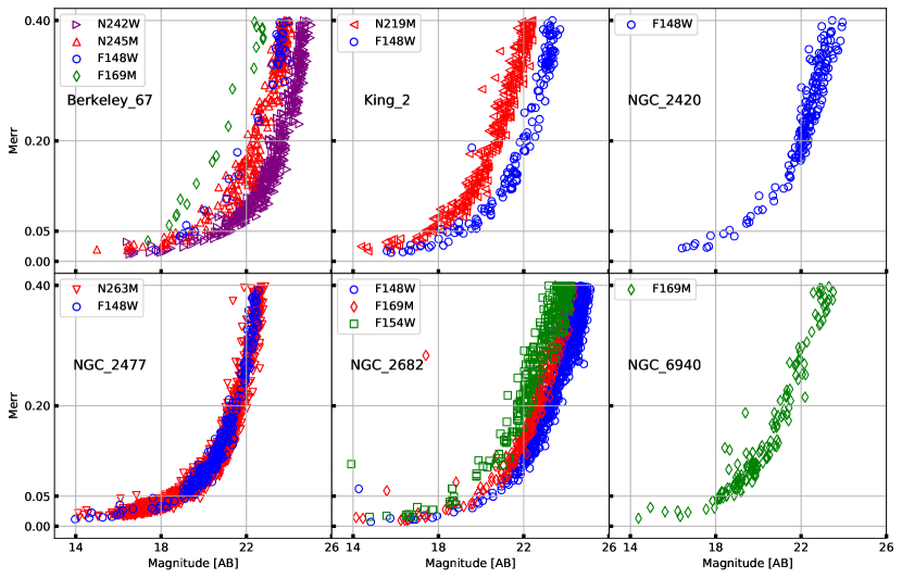
Figure 9: The photometric error in the magnitudes. Each subplot shows the magnitude-error plots for a cluster in all available filters. Please refer to the electronic version of the journal for the colour version.

We performed PSF photometry on all UVIT images using daophot package of iraf. We used 5-$\sigma$ detection and limited the catalogue up to the detection with magnitude errors $<$ 0.4 mag. The magnitude vs PSF error plots for all the images are shown in Fig. 9. The magnitudes were corrected for saturation following Tandon et al. (2017). We removed artefacts arising from saturated/bright stars and false detection at the edge, to create the final list of UVIT detected sources for each observed filter. We included the saturated stars in the catalogue, however their magnitudes represent the upper limit (they are brighter than these values), and their astrometry may be incorrect by a few arcseconds. In this way, over 100 stars were detected in each image and the details of this are listed in Table 2.

2.2 Gaia data

The Gaia EDR3 data for all clusters were compiled by constraining spatial and parallax measurements. We used the r50 (radius containing half the members) mentioned in Cantat-Gaudin et al. (2020) to get the majority of the members with minimal contamination in the VPD. This region was used to calculate MPs in the gmm model. We tripled the radius for running the prf algorithm to detect more members in the outer region. The definition and formulae of independent/derived Gaia parameters used in this work are shown in Table 3. The errors of ra, dec, pmra, pmdec and parallax are taken from Gaia EDR3. Upper limits of the photometric errors in g are calculated using the ‘mag_error’ formula in Table 3 (similar for errors in gbp, grp, bp_rp bp_g and g_rp). Errors in ruwe and aen are assumed to be zero.

The parallax_cluster, ra_cluster, dec_cluster and radius_cluster (as mentioned in Table 1) are used to select sources near cluster using following ADQL query:   select *
from gaiaedr3.gaia_source
where
pmra is not null and parallax is not null and
ABS(parallax-cluster_parallax)$<$3* parallax_error and
contains(point(’icrs’, gaiaedr3.gaia_source.ra, gaiaedr3.gaia_source.dec), circle(’icrs’, cluster_ra, cluster_dec, cluster_radius)) = 1  

2.3 Isochrones and evolutionary tracks

We used parsec isochrones (Bressan et al., 2012) generated for cluster metallicity and age, adopted from Dias et al. (2002) and WEBDA. We used Kroupa (2001) initial mass function for the isochrones. As the UV images would detect WDs, we included WD (hydrogen rich atmosphere, type DA) cooling curves in the CMDs. We used tracks by Fontaine et al. (2001) and Tremblay et al. (2011) for Gaia filters and UVIT filters (Bergeron P., private communication). As the turnoff masses of the OCs under study range from 1.1 to 2.3 M_⊙, we included WD cooling curves of mass 0.5 to 0.7 M_⊙ (Cummings et al., 2018). The extinction for all filters was calculated using Cardelli et al. (1989) and O’Donnell (1994). We used reddened isochrones and WD cooling curves in this paper.

3 Membership Determination

3.1 Gaussian Mixture Model

The distribution of stars in the PM space is assumed to be an overlap of two Gaussian distributions. The sum of which can be written as,

$$f(\mu|\overline{\mu_{j}},\Sigma_{j})=\sum_{j=1}^{2}w_{j}\frac{exp\left[-1/2(\mu-\overline{\mu_{j}})^{T}\Sigma^{-1}_{j}(\mu-\overline{\mu_{j}})\right]}{2\pi\sqrt{det\Sigma_{j}}}$$ (1)

$$w_{j}>0,\qquad\sum_{j=1}^{2}w_{j}=1$$ (2)

where $\mu$ is individual PM vector, $\overline{\mu_{j}}$ are field and cluster mean PMs, $\Sigma$ is the symmetric covariance matrix and $w_{j}$ are weights for the two Gaussian distributions. The generalised formalism for the n-D case and details of fitting the Gaussian distributions to Gaia data are available in Vasiliev (2019) appendix.

We selected stars within r50 of cluster centre and removed sources with following quality filters (Lindegren et al., 2018; Riello, Marco et al., 2020) to keep stars with good astrometric solutions:

$$\begin{split}\textsc{ruwe}>1.4\\ \textsc{aen > 1.0}\quad\textsc{and}\quad\textsc{aen\_sig > 2.0}\\ |\textsc{parallax}-parallax\_cluster|>3\times\textsc{parallax\_error}\end{split}$$ (3)

For such sources, a gmm is created using pmra and pmdec, as only these parameters have distinct Gaussian distribution for the cluster members. Two isotropic Gaussian distributions are assumed for the field and member stars, which were initialised with previously know values of cluster PM and internal velocity dispersion. We used GaiaTools to maximise the likelihood of the gmm and get mean and standard deviation of the two Gaussian distributions. Simultaneously, the MPs of all stars in the field are calculated.

gmm cannot use the other parameters provided by Gaia EDR3 catalogue (parallax, ra, dec, g, bp_rp, etc.) due to their non-Gaussian distributions. gmm does not organically account for systematic parameters leading to loss of interesting stellar systems with variability, binarity and atypical spectra. However, gmm can convincingly give the average CMD and VPD distribution of stars in a cluster. This can be further enhanced with the inclusion of photometric and systematic information. Hence, we used a supervised ML method to improve membership determination and utilise the non-Gaussian parameters.

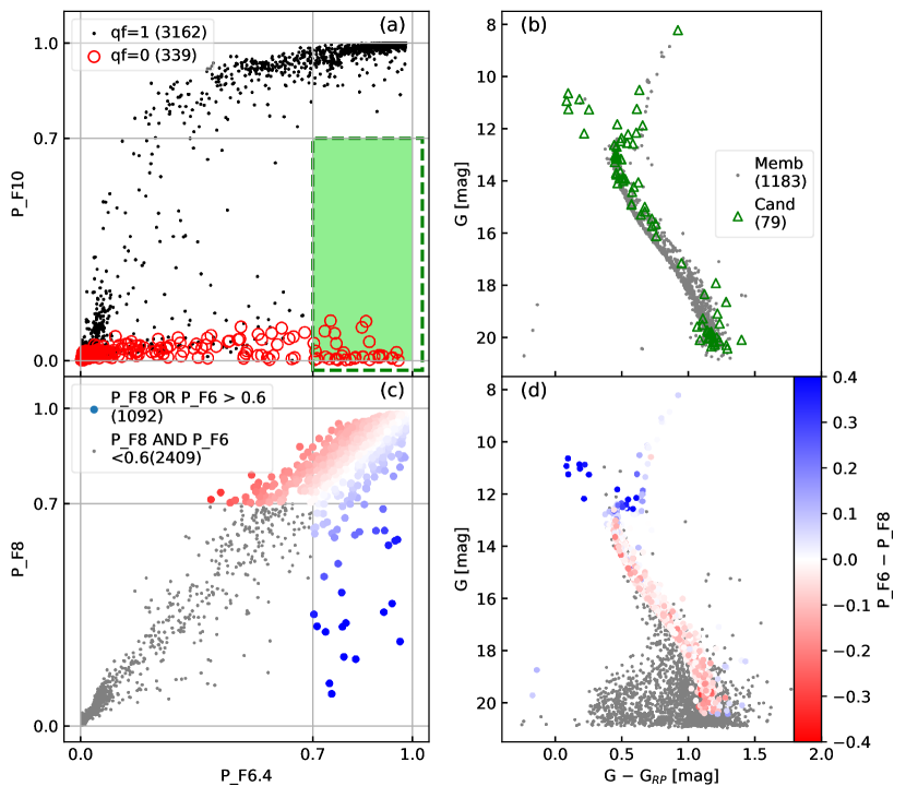
Figure 1: Comparison of different MPs from prf feature-combinations for NGC 2682. The numbers in brackets represent the number of stars in that particular category. (a) Comparison of F6 and F10, where black dots are good quality sources (qf = 1) and red circles are poor quality sources (qf = 0). The green dashed box represents sources with $P\_F10<0.7\leq P\_F6$. (b) CMD of NGC 2682 according to membership criteria in Eq. 5, the grey dots are members ($P\_F10>0.7$), while the green triangles are the candidates ($P\_F10<0.7\leq P\_F6$). (c) Comparison of F6 and F8 to demonstrate the MP dependence on CMD location. The colour is according to (P_F6 $-$ P_F8), as shown in the right most panel. (d) CMD of stars coloured according to (P_F6 $-$ P_F8). The stars with peculiar CMD position are bluer.

3.2 Probabilistic Random Forest

A random forest consists of multiple decision trees. Each decision tree consists of nodes, where the values of the features are compared with thresholds. These thresholds are optimised in the training phase by using a sample of known sources, each with a given set of features (e.g. photometry, astrometry, etc.) and labels (member, non-member). The decision trees repeatedly split the sample up until only one class of source remains at the end of each split. Finally, the average classification of all the decision trees is used, each of which is trained on different subsets of the sample.

The major drawback of traditional random forest is that there are no uncertainties (errors) assumed during these calculations. The probabilistic random forest (prf) algorithm , developed by Reis et al. (2019), takes care of errors in the data, which is essential for any astronomical data-set. It assumes all features and labels as probability distribution functions and out-performs traditional random forest algorithms in case of noisy data sets.

To create a training set for the prf algorithm, we first calculated the MPs using the gmm method. We used stars within r50 radius (Cantat-Gaudin et al., 2020) from the cluster centre to reduce field star contamination. The training set was created for each cluster by labelling $P\_GMM>0.5$ as members and others as non-members. The training set and testing set were created by randomly splitting the data set in 3:1 ratio, respectively. The prf requires the features, their errors and the known class (gmm membership labels) as inputs for training. The output contains fractional MP for each star and the feature-importance. After training the prf on stars within radius r50, we applied the algorithm on the stars within 3$\times$r50 of cluster centre to increase the sample size.

We assessed the performance of the following parameters, as features which can impact the membership determination: ra, dec, pmra, pmdec, parallax, g, g_rp, ruwe, aen, pmR0 and many others. The meaning of the features used are mentioned in Table 3. Radial velocities (RVs) are limited to stars with g $<15$; hence they were not used as a feature.

We tried more than 22 feature-combinations to optimise the membership determination. We judged the different combinations by:

1. their ability to recreate MP similar to gmm using ‘accuracy score’ in testing phase. The accuracy score is defined as:

   $$accuracy\ score=\frac{correctly\ predicted\ class}{total\ testing\ class}\times 100$$ (4)

   Although the accuracy score itself is not enough to select the final feature-combination, one can weed out poorly performing combinations.

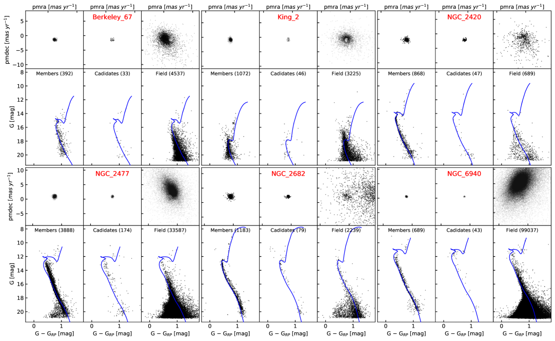
Figure 10: VPDs and CMDs of the six clusters. First and third rows are VPDs of members, candidates and field for respective clusters. Second and fourth rows are CMDs of members, candidates and field for respective clusters. Isochrones are plotted as blue line for reference.

2. the distribution of members in VPDs (Cluster should occupy compact circular region in the VPD e.g. Fig. 10).

3. the distribution of members in CMDs (Minimal contamination to the CMD, although it is a subjective judgement).

4. the distribution of members in PM–parallax plot (Cluster should occupy small range in both PM and distance).

Based on their individual merits, the notable feature-combinations are listed in Table 4.

Table 4: Feature-combinations used in prf algorithm to calculate MP.

Name	Features	Information
F6	ra, dec, pmra, pmdec, parallax, pmR0	Astrometry
F8	ra, dec, pmra, pmdec, parallax, pmR0, g, g_rp	Astrometry+ Photometry
F10	ra, dec, pmra, pmdec, parallax, pmR0, g, g_rp, ruwe, aen	Astrometry+ Photometry+ Systematics

3.3 Selection of features and membership criteria

We trained prf using 1 to 1000 trees and saw a plateau in accuracy score after 150–200 trees. As Oshiro et al. (2012) suggested, the optimum number of trees lies between 64–128, hence we chose 200 trees for further analysis. Almost all feature-combinations had an accuracy score of 92–98%, as all were designed to select the cluster members. Hence, choosing the best combination is not trivial.

As expected pmra, pmdec and parallax are important features for membership. The cluster’s distribution in VPD is Gaussian, and the random forest does not completely replicate this quadratic relation between pmra and pmdec. Hence we created a new parameter called pmR0, which is the separation of the source from the cluster centre in the VPD. The PM cluster centre was obtained from the gmm results. pmR0 helped constrain the cluster distribution to a circular shape. To test the importance of individual features, we introduced a column with random numbers as a feature. Among the Gaia features, ra and dec showed very comparable feature-importance as the random column. However, upon further inspection, we found that inclusion of ra/dec does not harm the prf while improving the membership determination (King 2 is an example, which is the farthest cluster in our set and has smallest sky footprint). Due to known overestimation of gbp flux in fainter and redder stars (Riello, Marco et al., 2020), we used g and g_rp as features.

We added ruwe and aen as features to include the quality checks in prf. This nullifies the need for manually filtering the data. The sources with large ruwe/aen are typically binary stars, variables, extended sources or stars with atypical Spectral Energy Distribution (SED; Lindegren, Lennart et al. 2020; Riello, Marco et al. 2020; Gaia Collaboration et al. 2020; Fabricius, Claus et al. 2020. As binaries and atypical SEDs are an important part of the clusters, we devised a method to keep such poor quality sources as candidates. Hereafter, we will refer to sources with qf = 1 as ‘good quality sources’ and sources with qf = 0 as ‘bad quality sources’. Feature-combination F6 uses only astrometric data (see Table 4) for the membership determination, hence it can give the MPs for poor quality sources. F10 uses astrometric, photometric and systematic parameters as features, hence it can give membership of good quality sources. Fig. 1 (a) shows the comparison of MPs from F6 and F10. As seen from the CMD in Fig. 1 (b), the bad quality sources in green region (P_F10 $<$ 0.7 $<$ P_F6) are very good candidate to be cluster members. For further text we define the members, candidates and field, as follows:

$$\begin{split}\texttt{Members}\Rightarrow{}&P\_F10>cutoff\\ \texttt{Candidates}\Rightarrow{}&P\_F10<cutoff\leq P\_F6.4\\ \texttt{Field}\Rightarrow{}&P\_F10\ \textsc{and}\ P\_F6<cutoff\end{split}$$ (5)

In an ideal scenario without systematic errors, we would use only F6 for the membership. We recommend using the candidate classification for G $<$ 19 (large intrinsic errors at fainter magnitudes create spread in bottom MS). After looking at the CMDs and residual VPDs with various cutoffs, we recommend cutoff of 0.7. However, we note that the ideal cutoff varies from cluster to cluster and strongly depends on the separation of cluster–field in the VPD and ratio of field stars to cluster members.

While analysing the different feature combinations, we found that adding photometric information (F8) to astrometric information (F6) leads to lessening the MP of stars in peculiar CMD locations. This is demonstrated in Fig. 1 (c) and (d). Most stars have the same MP from F8 and F6, however, the BSSs in NGC 2682 have larger P_F6 $-$ P_F8, due to absence of many stars in the same location in the training set. For further discussion, we will refer to (P_F6 $-$ P_F8) as peculiarity. Unfortunately, other clusters do not have many BSSs, the peculiarity can be used to distinguish between stars on the MS and sub-giant/giant branch.

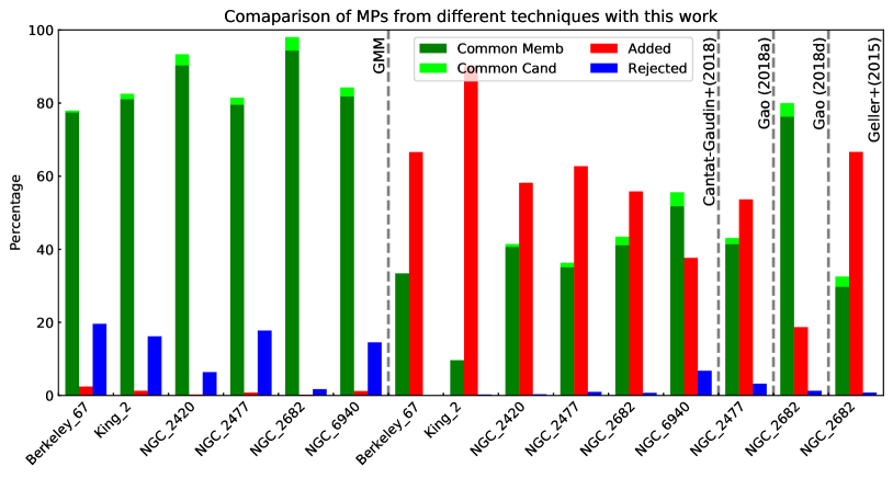
Figure 2: Grouped histogram for common candidates, common members, added members and rejected stars. The totals of four classes are normalised to 100 for easy visualisation and the numbers are tabulated in Table 5. The likely members by prf and other techniques are represented by Common Memb (dark green) and Common Cand (lime). Red bars are stars added as members by prf (classified as field by other techniques or missing from literature catalogues). Blue bars are stars rejected (classified as field) by prf but these are members in other techniques. Most of the rejected stars are faint and with larger pmR0. The dotted lines separate the comparisons with different methods and papers viz. gmm, Cantat-Gaudin et al. (2018), Gao (2018a), Gao (2018d) and Geller et al. (2015). All comparisons are done for the same field of view.

Table 5: Comparison of membership classification by prf with gmm, Cantat-Gaudin et al. (2018), Gao (2018a), Gao (2018d) and Geller et al. (2015).

	Common	Common	Added	Rejected
	Memb	Cand	Memb	Stars
	[1]	[2]	[3]	[4]
Comparison with gmm
Berkeley 67	158	1	5	40
King 2	506	9	8	101
NGC 2420	354	12	1	25
NGC 2477	1416	33	14	316
NGC 2682	436	17	1	8
NGC 6940	338	10	5	60
Comparison with Cantat-Gaudin et al. (2018)
Berkeley 67	131	0	261	0
King 2	104	0	968	3
NGC 2420	357	7	511	3
NGC 2477	1396	46	2492	39
NGC 2682	502	28	681	9
NGC 6940	399	29	290	52
Comparison with Gao (2018a)
NGC 2477	1695	67	2193	133
Comparison with Gao (2018d)
NGC 2682	950	46	233	16
Comparison with Geller et al. (2015)
NGC 2682	365	34	817	10
[1] Classified as members by both prf and other techniques
[2] Members of other techniques classified as Candidates by prf
[3] Added members by prf, which are not members in other catalogues
[4] Members from other techniques classified as field by prf

3.4 Comparison with literature

Fig. 2 shows the comparison of prf with gmm, Cantat-Gaudin et al. (2018), Gao (2018a) and Gao (2018d). The actual numbers of different types of stars are listed in Table 5. Although intuitive, the meaning of ‘added’, ‘rejected’ etc. is given in Table 5 footnote. Although Lindegren, Lennart et al. (2020) warns against direct crossmatch between DR2 and EDR3 due to changes in epochs, the astrometric shift for cluster members is $<$ 10 mas. All comparisons were done over the same field of view.

gmm and prf used different set of parameters. As seen Fig. 2, the classification by prf was similar to gmm. The accuracy score (reproducibility) of prf was between 90–99% for the six clusters. However, there are some differences, which are expected and embraced. The major difference was seen in the rejection of gmm members (2–25%), most of which were in G $>$ 19 mag region. Among stars brighter than 19 mag, the percentage of rejected stars drops to 0–4%, almost all having poor astrometric solutions (ruwe $>1.2$).

Cantat-Gaudin et al. (2018) used clustering in the ($\mu_{\alpha},\mu_{\delta},\pi$) space to identify the members using Gaia DR2 data. They selected the stars with parallax within 0.3 mas and PM within 2 mas year^-1 of the cluster mean. The probabilities were calculated using upmask, an unsupervised clustering algorithm. prf has identified significantly more (260-2500) new members compared to Cantat-Gaudin et al.. All the added stars have acceptable CMDs, VPDs and PM–parallax distributions. As the magnitude limit of Cantat-Gaudin et al. catalogue was 18, many new members are added in the fainter end of the MS. The rejected members (0–52) typically have either high ruwe/low pmR0 or low ruwe/high pmR0. As the added stars far outnumber the rejected stars, this is a good optimisation.

Gao (2018a) used Gaia DR2 to determine membership of NGC 2477 (and three other clusters) using a gmm. Although there are 1695 common members, prf has added 2193 stars and rejected 133 stars. Majority of added stars are near the cluster parallax and pmR0 $<$ 1.5 mas yr^-1. The rejected stars are again typically results of ruwe/aen and pmR0 trade-off.

Gao (2018d) utilised a random forest of 11 Gaia parameters (ra, dec, parallax, pmra, pmdec, g, gbp, grp, bp_rp, bp_g and g_rp ) to calculate the MPs of NGC 2682. Gao did not remove stars with high systematic errors, and the random forest algorithm did not incorporate uncertainties in the astrometric data. The use of EDR3 data, inclusion of errors and using the F6 and F8 feature-combinations has led to 233 more members. Geller et al. (2015) calculated the MPs in NGC 2682 using a combination of RV measurements (up to 40 yr baseline) and previous PM data (Yadav et al., 2008). Their catalogue is magnitude limited due to its spectroscopic nature. Among the crossmatched Geller et al. members, we classify 3% stars as field, due to larger ruwe or different PM/parallax.

Comparison with previous literature confirms that F10 membership is adequate for membership, and we will use F10 as primary membership criteria. Due to the limitations (systematic and statistical errors) in Gaia EDR3, we included the candidate classification to account for the likely cluster members (using F6). We used both members (selected from F10) and candidates (selected from F10 and F6) for further analysis.

Importantly, our method was able to add a significantly large number of stars in all the clusters, ranging from 200–2500 stars per cluster (Table 5). Therefore, this is a significant improvement over the previous studies using Gaia DR2, mostly in the faint MS. This will certainly help in the detailed analysis of the clusters and locate interesting candidates that are bright in the UV.

4 Results

Table 6: The cluster parameters as derived from the members (see Eq. 5) of the six clusters.

Cluster	Berkeley 67	King 2	NGC 2420	NGC 2477	NGC 2682	NGC 6940
Total stars in 3$\times$r50	4962	4343	1604	37649	3501	99769
Members	392	1072	868	3888	1183	689
Candidates	33	46	47	174	79	43
ra_mean [degree] α	69.471	12.727	114.603	118.048	132.844	308.632
dec_mean [degree] α	50.743	58.186	21.577	$-$38.534	11.827	28.300
pmra_mean [mas yr-1] α	2.28$\pm$0.28	$-$1.43$\pm$0.27	$-$1.22$\pm$0.30	$-$2.43$\pm$0.26	$-$10.96$\pm$0.33	$-$1.96$\pm$0.15
pmdec_mean [mas yr-1] α	$-$1.42$\pm$0.22	$-$0.85$\pm$0.35	$-$2.05$\pm$0.26	0.90$\pm$0.27	$-$2.91$\pm$0.29	$-$9.44$\pm$0.16
Stars with RV	2	1	6	16	39	15
RV_mean [km s-1] α	$\sim$ $-$1	$\sim$ $-$41	73$\pm$2	8$\pm$4	34$\pm$4	8$\pm$4
parallax_mean [mas] α	0.43$\pm$0.29	0.15$\pm$0.39	0.38$\pm$0.26	0.64$\pm$0.33	1.16$\pm$0.28	0.95$\pm$0.19
distance from isochrone [pc]	2023	5749	2512	1514	848	1000
R_core [′] β	1.3	0.5	1.2	6.4	6.3	2.2
R_core [pc]	0.76	0.84	0.88	2.82	1.55	0.64
α The means and errors are mean and standard deviations of Gaussian fit to the member parameters.
β Projected R_core is calculated using distance from isochrone fits

4.1 The Catalogues

The results of this study are presented in the form of seven catalogues, a membership catalogue and six catalogue of UVIT photometry. The membership catalogue (for sources with $P\_F6\ \textsc{or}\ P\_F10>0.1$) contains Gaia EDR3 astrometry and photometry (ra, dec, g, g_rp), MPs (P_GMM, P_F6, P_F8 and P_F10), quality filter (qf) and membership classification (M: member, C: candidate and F: Field). The example of the catalogue is given in Table 7 (full version is available online). Table 8 shows the example of UV catalogue of NGC 6940, which is observed in F169M filter. The full catalogues of six clusters are available online. The catalogues contain R.A.(J2016), Dec.(J2016), UV magnitudes, magnitude errors, MPs (P_F10 and P_F6) and membership classification (M: member, C: candidate and F: Field). We have included saturated stars in the catalogue, whose magnitudes give the upper bound to the actual numerical value.

We cross-matched the Gaia and UVIT catalogues with a radius of 1^′′, to get merged catalogues using topcat. We checked for crowding and issues during cross-matching process (e.g. duplicity), but both Gaia and UVIT catalogue showed an insignificant number of stars within 1^′′ of each other (2 for all UVIT detections and $<$ 0.4% in Gaia detections). These merged catalogues were used for further analysis.

4.2 Cluster properties

We derived following mean cluster properties by fitting Gaussian distribution to the members: R.A., Dec, parallax, PM and RV. Additionally, we included distances calculated by isochrone fitting. We removed a few outliers while calculating the mean parallax and RV. We fitted King’s surface density profile to cluster surface density.

$$\rho(R)=F_{bg}+\frac{F_{0}}{1+(R/R_{core})^{2}}$$ (6)

where $F_{bg}$ is background counts, $F_{0}$ is count in the bin, R is the RMS of each bin limits (in degree) and $R_{core}$ is the core radius. We binned the members such that the bin area was constant for each bin in the spatial plane. This method decreased the thickness of bin as we moved outwards from the cluster centre. The smallest bin width was kept equal to the mean separation between nearby members, and the rest of the bins were scaled accordingly. The $F_{bg}$ was assumed to be nil for the profile fitting.

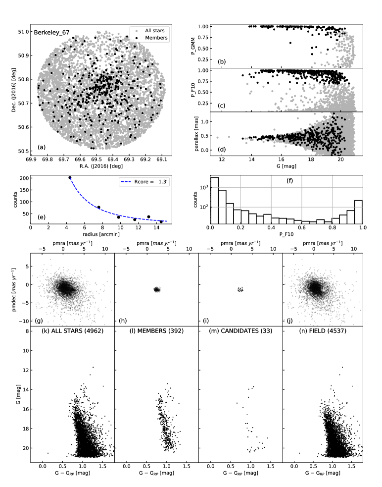
Figure 11: (a) Spatial distribution for Berkeley 67. All Gaia stars are denoted by grey dots and cluster members are denoted by black points. (b)–(d) Distribution of g magnitude with P_GMM, P_F10.3 and parallax. (e) Calculation of core radius by fitting radial density with King’s surface density profile. (f) Histogram of P_10.3. The bimodal Moffat profile is shows with dashed curve, while the minima of the profile is represented by dot-dashed line. (g)–(j) and (k)–(n) show the VPD and CMD of all stars, members, candidates and field respectively. (k)–(n) show the number of stars plotted in the brackets along with the Padova isochrone as a blue curve.

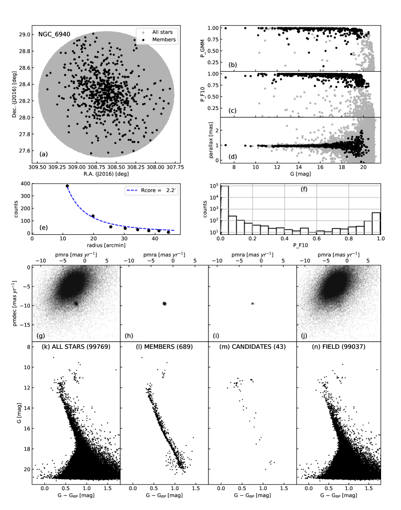
Figure 16: Spatial distribution, VPD and CMDs of NGC 6940. The subplot descriptions are same as Fig. 11.

All the parameters are tabulated in Table 6. Gaia EDR3 sources near each cluster are are divided into three subsets: members, candidates and field. The VPDs and CMDs of all clusters for these individual subsets are shown in Fig. 10. The spatial distribution, VPD, CMD, g vs MP etc. for clusters is shown in Fig. 11 to Fig. 16. For each cluster, Fig. (a) shows the spatial distributions of members and non-member population. Fig. (b) and (c) show the distribution of GMM and F10.3 probabilities as a function of g. We expected clear separation between members for bright stars, which is seen in all the clusters up to 16–18 mags. Fig. (d) shows the distribution parallax as a function of g. All clusters, except King 2, show a peak in parallax for the member stars. Fig. (e) shows the King’s surface density profile fitted to members’ surface density. Fig. (f) shows the histogram of F10 MP. Fig. (g) and (k) show the VPD and CMD for all stars. Fig. (h) and (l) show the VPD and CMD for members. Fig. (i) and (m) show the VPD and CMD for candidates. Fig. (j) and (n) show the VPD and CMD for field stars.

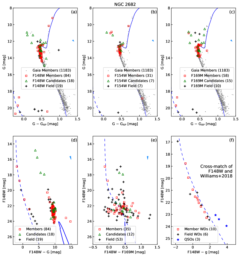
Figure 3: The CMDs of NGC 2682 with UVIT and Gaia photometry. Gray dots are Gaia EDR3 members according to Eq. 5. Red squares, green triangles and black crosses are members, candidates and field stars detected in particular filters. The blue line is an isochrone with $Log(Age)=9.6,DistanceModulus=9.64,E(B-V)=0.05\ mag,[M/H]=0\ dex$; the dashed blue line is WD cooling curve for a 0.5 M_⊙ WD; the light blue arrows represent the reddening vectors with direction and magnitude in each CMD. (a), (b) and (c) The optical CMDs with stars detected in F148W, F154W and F169M filters respectively. (d) The UV–optical CMDs with F148W and g filters. (e) The UV CMD with F148W $-$ F169M colour. (f) UV–optical CMD of sources cross-matched with Williams et al. (2018) catalogue of possible WDs. The CMD also shows three quasars (blue stars) detected by F148W filter.

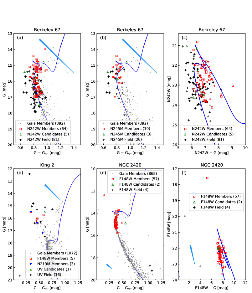
Figure 4: (a), (b) and (c) The optical and optical–UV CMDs of Berkeley 67. The markers are same as Fig. 3. The isochrones for Berkeley 67 has $Log(Age)=9.2,DistanceModulus=11.53,E(B-V)=0.8\ mag,[M/H]=0\ dex$. (d) Optical CMD of King 2. with F148W detected members denoted by red squares and N219M detected members denoted by blue filled triangles. The isochrones for King 2 has $Log(Age)=9.7,DistanceModulus=13.8,E(B-V)=0.45\ mag,[M/H]=-0.4\ dex$. (e) and (f) The optical and UV–optical CMDs of NGC 2420. The markers are same as Fig. 3. The isochrones for NGC 2420 has $Log(Age)=9.3,DistanceModulus=12.0,E(B-V)=0.15\ mag,[M/H]=-0.4\ dex$; WD cooling curve is for 0.6 M_⊙ WD.

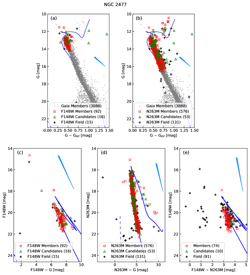
Figure 5: (a) and (b) The optical CMDs of NGC 2477. (c), (d) and (e) The UV–optical and UV CMDs of NGC 2477. The markers are same as Fig. 3. The isochrones is for $Log(Age)=8.9,DistanceModulus=10.9,E(B-V)=0.4\ mag,[M/H]=0\ dex$; WD cooling curve is for a 0.7 M_⊙ WD.

Figure 6: (a) and (b) The optical and UV–optical CMDs of NGC 6940. The markers are the same as Fig. 3. The isochrones is for $Log(Age)=9.0,DistanceModulus=10.0,E(B-V)=0.2\ mag,[M/H]=0.0\ dex$; WD cooling curve is for a 0.6 M_⊙ WD.

4.3 Individual clusters

NGC 2682 has a prominent binary sequence, red giant (RG) branch and BSS population (Fig. 10). We detected many candidates as BSSs, MS stars and a few RG stars. The MS candidates typically have $\textsc{qf}=0$. The optical CMDs of stars detected in the FUV filters are shown in Fig. 3 (a), (b) and (c). The CMDs contain all Gaia members, UVIT detected sources, isochrone and WD cooling curve of 0.5 M_⊙. Overall, we detected 84, 31 and 58 members in F148W, F154W and F169M respectively. Fig. 3 (d) shows the UV–optical CMD of sources cross-matched between Gaia EDR3 and F148W. The turnoff of the isochrone lies at 24 mag, which is the limiting magnitude of F148W observations. All the stars on optical MS are located above the turnoff in UV–optical CMD. Hence, as previously seen in Jadhav et al. (2019), almost all MS stars detected in optical CMD have FUV excess. The photometry presented here is two magnitudes fainter than Jadhav et al. (2019) in F148W, and we have detected a good number of MS stars in the 22 to 24 magnitude range, with FUV excess. Fig. 3 (e) shows the F148W, (F148W $-$ F169M) CMD (the MS/turnoff is the vertical line at $\sim$ 0.5 colour). The sources show a large spread in FUV colour, ranging from 0.0 to 1.3 mag.

FUV images can be used to detect WDs. However, as they are faint in the optical wavelengths, Gaia is not suitable to detect them. In order to effectively identify the WDs, we cross-matched the F148W detected sources with the WD catalogue of Williams et al. (2018). Fig. 3 (f) shows the CMD of all cross-matched sources and the WD cooling curve. The membership information and g-band photometry (for this subplot alone) are taken from Williams et al. (2018). F148W has detected ten member WDs, six field WDs and three quasars. All these sources follow the WD cooling curve.

Berkeley 67’s VPD (Fig. 10) shows that the mean cluster motion and mean field motion are within a few mas year^-1 of each other. The cluster has only $\sim$ 400 members; hence there is not much over-density in the VPD. Thus, it is particularly challenging to determine the membership for Berkeley 67. The CMD shows a large spread in the MS. We suspect the large spread is the result of the differential reddening in the cluster region, whose effect is enhanced by the high extinction towards the cluster. UVIT images of Berkeley 67 in F148W (exp. time = 2683 s) and F169M (exp. time = 1317s) filters detected no member stars. Therefore, the cluster does not have any FUV bright members. N242W and N245M images detected 64 and 19 members respectively. We did not detect any BSS. Fig. 4 (a) and (b) show the Gaia CMDs of these NUV detected members. We observe turnoff stars in both NUV filters, with the wider N242W filter going till 17 mag. N242W filter detects two RGs which are rarely detected in the UV regime. Fig. 4 (c) shows the N242W, (N242W $-$ g) CMD for Berkeley 67, which again confirms the large scatter.

King 2 is the farthest cluster included in this work. This is evident from the small apparent core radius (0.^′5) and high feature-importance for ra and dec. The parallax measurements are unreliable at the distance of $\sim$5 kpc. The cluster and field centres in the VPD are very close and hence, there may be contamination from field stars, among the members. Nevertheless, there are many BSSs and red clump stars present in the cluster (Fig. 10). We detected 5 and 3 members each inF148W and N219M filter respectively (Fig. 4 (d)). This 5 Gyr old cluster located at a large distance has the MS turnoff at 18 mag (in g-band) and hence we detected only the brightest of BSSs in UV. Overall, there are 5 member BSSs and 1 candidate BSS in UV images. Two of the BSSs have both FUV and NUV detections. We detect one blue and faint (g-band) object, which is likely a foreground WDs.

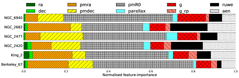
Figure 7: Normalised feature-importance for F10 for all six OCs.

NGC 2420 lies in a relatively less dense region with the field to member stars ratio of $\sim$ 1 (Fig. 10). It has a clearly defined binary sequence and a RG branch, with a few BSSs. The UVIT image has stars up to two magnitudes below the MS turnoff, including a BSS. The UV CMD shows that the candidates are located close to the turnoff, though they are much fainter in the optical CMD, suggesting a brightening in the UV. However, the excess UV flux is not as prominent as NGC 2682. Similarly, a few members also show UV excess flux, but the change in the magnitude is not as large as in NGC 2682.

NGC 2477 is a very dense cluster in a high stellar density region (38000 stars and 3900 members in 18 ′ radius). The Gaia CMD shows a well defined binary sequence, RC stars and $\sim$ 5 BSSs. The turnoff has a large spread in g-band. There is spread in the members below 18 mag, indicating that the probability cutoff should be slightly higher than 0.7. We detected 92 and 576 members in F148W and F263M respectively (Fig. 5 (a) and (b)). Fig. 5 (c) shows the F148W, (F148W $-$ g) CMD with 2 BSSs and MSTO stars. Fig. 5 (d) shows the N263M, (N263 $-$ g) CMD with a large range in NUV magnitude consisting of red clump stars and MS stars. Fig. 5 (e) shows the F148W, (F148W $-$ N263M) CMD, here we see the turnoff stars and many field stars with bluer UV colour.

NGC 6940 is situated in a very dense stellar environment (stellar density is 13 times that of NGC 2682 neighbourhood). The cluster is well separated from the central field in the VPD and has a significant parallax ($\sim$ 1 mas), hence it is easy to extract (Fig. 10). The CMD shows a clear binary sequence and red clump stars. NGC 6940 also has a relatively broad MS with a spread near its turnoff, although less prominent compared to NGC 2477. We detected members up to 2 magnitudes below turnoff (Fig. 6 (a)) including a giant. We did not detect any BSS in this 1 Gyr old cluster.

5 Discussion

5.1 Membership Determination

There are multiple ways of determining memberships. The choice of method is mainly dictated by the aim of the study. Any simple method such as VPDs for membership estimation is adequate for studies requiring the estimation of cluster parameters such as mean PM, age and distance. Here, our objective is to identify UV bright member stars in OCs, that could be in non-standard evolutionary stages. This requires the implementation of rigorous methods to assign membership to such stars, as discussed below:

Feature-importance: The prf method gives the importance of each feature as one of the results during the training phase. The normalised feature-importance is shown in Fig. 7. The most important features are pmR0, ruwe, aen, pmra, pmdec and g. The distance of the stars from the cluster centre in the VPD, pmR0, is an important feature as expected. The high importance of ruwe/aen is because they are cutoffs established during the training of the algorithm. The g importance is aided by the dependence of all errors on the magnitude. The ra/dec importance is more for King 2 and NGC 2420 when compared to other clusters. They have core radii of 0.^′5–1.^′2, while other clusters are typically larger. The smaller spatial distribution of members is causing an increase in the importance of ra/dec. As expected, the importance of parallax increases for nearby clusters (NGC 2420, NGC 2477, NGC 2682 and NGC 6940).

Efficacy in various environments: The prf technique works for OCs with a diverse cluster-members to field-stars ratio (0.01 to 1.3), thereby helping in efficient detection of members. The presence of systematic errors and including CMD locations through magnitude and colour tends to remove poor quality as well as peculiar stars. Therefore, we introduced the candidate classification to list such stars. For these six clusters, we found the candidates to members ratio to be 0.04–0.08.

Versatility of the technique: The algorithm is adaptable, and one can choose a particular feature-combination depending on the requirements. For example, for a statistical study of clusters, a feature combination with ra, dec and parallax would be enough. To find peculiar stars in the CMD, one could measure the difference between F6 (ra/dec, pmra/pmdec, parallax and pmR0) and F8 (F6 + g and g_rp). Peculiar stars typically have lower P_F8. The prf technique can also be applied to any data-set besides Gaia EDR3. Moreover, the inclusion of ruwe/aen as features indicates any systematic terms, if present in any other data-set, can also be incorporated in the algorithm.

Classification of BSSs: In the field of NGC 2682, there were 10 potential BSSs (bluer and brighter than the turnoff). prf classified two as members, six as candidates and two as field. Many of these stars are photometric variables or binaries (Geller et al., 2015), which can lead to high ruwe and hence classification as candidates. The two field stars have cluster parallax and RV (not considered as a membership criteria in prf). However, they have larger pmR0 leading to their rejection as members. For such stars with large PM deviation from the cluster mean, deeper RV measurements and accurate parallax will be useful in constraining membership. High peculiarity in combination with high ruwe of the BSSs is the reason for these stars to be categorised as candidates. Hence, the technique (Eq 5) is capable of selecting BSSs (albeit as candidates).

Existence of Candidate class: All the cluster candidates lie near the cluster centre in the VPDs. Their number increases as they get fainter; this mirrors the fact that the systematic errors in Gaia EDR3 are larger for fainter stars. The CMD of NGC 6940 candidates (Fig. 10) shows that the majority of them lie on the binary sequence. A similar but lesser effect is seen in NGC 2477 and NGC 2682. Binary systems are known to produce high ruwe values due to variability or unsymmetrical PSF (Deacon & Kraus, 2020), hence they can have low P_F10 and get classified as candidates.

Detection of peculiar stars using multiple feature-combinations: In Fig. 1 (e), we compared the MPs with and without g and g_rp as features (F8 and F6 respectively). F6 has no knowledge of CMD positions, so it uses only spatial location and velocity to classify stars. However, F8 selects stars with common CMD positions and rejects stars with uncommon CMD positions. This effect is demonstrated by the positive values of $P\_F6-P\_F8$ for BSSs in NGC 2682 (Fig. 1 (d)). We refer to large $P\_F6-P\_F8$ as peculiarity. Such peculiarity can be seen for the BSSs in NGC 2682, NGC 2477 and King 2. However, for King 2 majority of stars bluer than bp_rp $<$ 1.1 mag have similar peculiarity regardless of their magnitude. Other clusters in this study do not have many BSSs and they only showed large $P\_F6-P\_F8$ near limiting magnitude.

5.2 Individual clusters

NGC 2682: The detection of stars on the MS in the UV CMDs, suggests that many MS stars have excess UV flux. Jadhav et al. (2019) presented the reasons for UV excess such as the presence of hot WD components, chromospheric activity and hot-spots on contact binaries. Such UV excess detected among the MS stars is unique to NGC 2682; as for all other clusters, only a few stars on the MS show UV excess. In Fig. 3 (a) and (d), a few WD members and many field stars are found near the WD cooling curve. The CMD location suggests these can be WDs. Their MPs are low due to astrometric and photometric errors. As NGC 2682 is a well studied OC, we used deep photometric catalogue of Williams et al. (2018). They identified hot and faint stars in u,(u $-$ g) plane and carried out spectroscopic observations to confirm the WDs from their atmospheric signatures. We cross-matched all F148W detections with Williams et al. (2018) catalogue and found ten member WDs and six field WDs, along with the three quasars. Therefore, UVIT observations are well suited to detect WDs in NGC 2682.

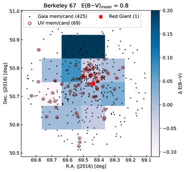
Figure 8: Spatial location of RGs in Berkeley 67 over-plotted on the reddening map. The plot contains all Gaia members/candidates (as black dots), N242W members/candidates (as red circles) and the RG detected in N242W filter (as red square).

Berkeley 67: The cluster has very high reddening (E(B $-$ V) = 0.8 mag). Thus, small relative changes in reddening have a substantial impact on magnitude/colour and cause a broadening of MS in the CMD. We tried binning the Gaia members spatially and analysed the distributions in the CMD plane. Initial estimates suggested that the E(B $-$ V) values have a range of 0.7 to 1.0 mag. The reddening map is shown in Fig. 8. We detected one RG member in NUV which lies in the low reddening region. Further investigation is needed to determine the exact cause of UV brightening of the RG. Fig. 4 (c) shows members distributed in MS and sub-giant branch. From the UV CMD, it indicates the spread at the optical turnoff can be due to subgiant stars or due to differential reddening. As the extinction vector is parallel to the subgiant branch, any differential reddening will increase the spread in the same direction.

King 2: As the oldest and farthest cluster in this work, only bright BSSs are detected by UVIT. Jadhav (2021; under review) presented the detailed analysis of the detected BSS population, including detection of Extreme Horizontal Branch/subdwarf B type stars as companions to BSSs.

NGC 2420: We detected the BSS present in the cluster in the UV. We found $\sim$ 6 stars (out of 59), located on the MS, to show signs of excess UV flux. Some stars are found at the turnoff, and three are candidates. One of the candidate has ruwe = 3.9 while the other has no Gaia colours. High ruwe is known to be caused by variability and/or binarity (Deacon & Kraus, 2020). The missing colour/high ruwe and excess UV flux points towards a hotter companion or variability. Multi-wavelength analysis and X-ray observations of these stars can shed light on their evolutionary status.

NGC 2477: We have detected a large number of stars in FUV (108) and NUV (629), hence it is ideal to study the UV properties from the MS up to the red clump. This massive cluster is also ideal to study the UV properties of stars in the broad MS turnoff present in this cluster. Overall the UV CMDs are aligned with the UV isochrones, not indicating a collective UV brightening alike NGC 2682 among the MS stars. However, there are a couple of stars showing considerable UV excess, which require multi-wavelength study.

NGC 6940: The UV CMD has some field stars near the WD cooling curve. These can be members or runaway WDs, which are quite faint in g. Some turnoff stars are found to be brighter than the turnoff in the UV CMD, suggesting excess FUV flux. We detected a giant with g = 7.3 mag and bp_rp = 3.7 mag in FUV at the limiting magnitude. It is a variable star of spectral type M5II-III D (Wallerstein, 1962). The isochrone suggests that this is likely to be a post-asymptotic giant branch (AGB) star. Due to the low temperature (T${}_{eff}^{Gaia}$ = 3355 K), the stellar continuum cannot emit detectable FUV flux. Further study is needed to characterise the emission mechanism.

5.3 General discussion for all clusters

WD detections: Cross-match of Williams et al. (2018) catalogue and Gaia EDR3 resulted in only 4 WDs in NGC 2682. While the cross-match with F148W resulted in detection of 16 WDs. The F148W image has detected stars up to 21.7 mag in g-band and 21.8 mag in u-band. This indicates that UV images are more suitable to detect hot WDs as compared to Gaia. CMDs of a few other clusters imply presence of photometric WDs: King 2 (Fig. 4 (d)), NGC 2477 (Fig. 5 (d)), NGC 6940 (Fig. 6 (b)). However, comparison with deeper catalogues is required for detecting WDs in these clusters. The membership determination of WDs is challenging due to deficiency of long-baseline deep observations in other open clusters. Although all the WDs have significant PM errors (Gaia EDR3 and Yadav et al. 2008), the spread in PM is clearly visible. It is interesting to note that three of the Gaia detected WDs in NGC 2682 lie at/just outside the edge of the cluster in the VPD.

Comparison of Gaia DR2 and EDR3: The membership analysis was done for both Gaia DR2 and EDR3. As EDR3 has halved the errors in PM, there were some changes in the members. EDR3 data has led to the addition of sources in the fainter end, which have PM similar to the cluster. We could probe the membership of all the stars in the cluster without any magnitude cutoff due to better accuracy in PM and inclusion of errors in the MP determination. The total percentage of candidates has dropped from 11% to 5%, and the VPD distribution of NGC 2682 members was elliptical in DR2 which is now circular in EDR3 data reflecting better handling of systematics in EDR3.

Future Improvements: There are scopes to improve the membership determination process in future based on the following points:

1. The use of RV can constrain the spatial motion of members, however deeper RV data is needed to get cluster membership for fainter stars.

2. The use of distance from the fiducial isochrone in the CMD could constrain the spread visible in the fainter region of the CMDs.

3. We miss some stars with slightly different space velocity, as the primary selection criterion is PM (e.g. 2 PM and RV members from Geller et al. 2015). Such stars are important to understand the kinematics of the cluster. Increasing the weightage and accuracy of parallax and CMD location can help identify such stars.

The method developed here is generic and can be applied to non Gaia data as well. We recommend a feature-combination similar to F8 (ra, dec, pmra, pmdec, pmR0, parallax/distance, photometric information) to constrain the spread in CMD and VPD. Additionally, comparison with equivalent F6 (Only astrometric information) will be helpful to identify peculiar stars in the CMD.

6 Conclusions and Summary

1. We developed an ML-based method to determine the individual stellar membership within OCs using Gaia EDR3. We have tried more than 22 different feature-combinations to calculate the MPs. The stars are classified as members, candidates and field using a combination of two prf methods. Our primary method (F10) identifies stars which have properties similar to the mean cluster properties and have small systematic errors as members. To incorporate peculiar stars (uncommon CMD locations) and stars with large systematic errors, we utilised another method (F6) which only uses spatial location and velocity coordinates. We compared and validated the performance of our methods with past membership studies. Additionally, we created a technique to identify stars with peculiar CMD position and demonstrated that it could identify BSSs.

2. We demonstrated that the prf algorithm could be used to determine the MPs in a variety of clusters. It is found to be robust, reproducible, versatile and efficient in various environments (variation in stellar density, reddening, age etc.). We have identified 200–2500 more cluster members, primarily in the fainter MS, compared to previous studies (which used Gaia DR2 data). The algorithm presented here is generic and could be changed to suit other data sets or scientific problems. It is editable by selecting different features or creating new features, as required.

3. We present a catalogue (Gaia EDR3 based) of six clusters which provides spatial location, MPs and classification in Table 7. The presence of candidate stars suggests a need for better astrometry and photometry, which will be available in future Gaia releases and other large scale surveys. We used the Gaia catalogue to identify cluster members in UVIT images. We present the UVIT catalogue of six OCs in one or more filters along with its membership information in Table 8 (full catalogues are available online). We estimated cluster properties such as mean PM, distance, mean RV and core radii from the identified member population.

4. We detected 3 to 700 member stars in various UVIT images of six clusters, apart from $\sim$13% candidates. We detected BSSs in King 2, NGC 2477, NGC 2420 and NGC 2682. FUV photometry presented here will be used to understand the formation pathways of BSSs. We also detected giant members in FUV (NGC 2682, NGC 6940) and NUV (Berkeley 67, NGC 2477). While most of the NUV detections are expected due to their luminosity and temperature, their FUV detections are unusual. We detected 10 WD members in FUV images of NGC 2682. UV CMDs indicates that there are a few possible WDs in NGC 2477, NGC 2682 and NGC 6940.

5. As seen in earlier studies, NGC 2682 has unusually high UV bright MS members. We detect no such systematic UV brightening among MS stars in other clusters. Some individual stars do show excess UV flux (RGs, a post-AGB star and a few MS stars). These are good contenders for detailed individual studies. The VPD of NGC 2682 is also notable due to its elliptical shape.

6. The massive cluster NGC 2477 has 92/576 members detected in FUV/NUV, which will be useful to study the UV properties of stars in the extended turnoff and various evolutionary stages from MS to red clump.

The UV and Gaia catalogues provide a comprehensive data set to inter-compare UV emission across various types of clusters and study stellar properties. We plan to perform a detailed analysis of the interesting sources identified in this study using panchromatic data (such as UVIT, Gaia EDR3 and X-ray) in future studies.

Data Availability

The Gaia EDR3 data is available at https://gea.esac.esa.int/archive/. The UVIT images can be accessed through https://astrobrowse.issdc.gov.in/astro_archive/archive/Home.jsp depending upon their proprietary period. The membership catalogue and UV photometric catalogues of six clusters are available at CDS via anonymous ftp to cdsarc.u-strasbg.fr (130.79.128.5).

Appendix A Open clusters under study

Berkeley 67 is a $\sim$1 Gyr old OC located at a distance of $\sim$2.45 kpc. It is a low-density cluster with an angular diameter of $\sim$14′. Lata et al. (2004) carried out deep Johnson UBV and Cousins RI CCD photometry of this cluster while Maciejewski & Niedzielski (2007) obtained BV CCD data as part of a survey of 42 open star clusters. Both studies are based on optical CMD of the cluster.

King 2 is a $\sim$5 Gyr old OC located at a distance of $\sim$6 kpc towards the Galactic anti-centre direction. It is a faint but rich cluster situated in a dense stellar field. It lags behind the local disc population by 60 to 100 km s^-1 and could be part of the Monoceros tidal stream (Warren & Cole, 2009). Kaluzny (1989) obtained BV CCD photometric data for the cluster. A deep Johnson–Cousins UBVR CCD photometric study of the cluster was carried out by Aparicio et al. (1990). They estimated E(B $-$ V) = 0.31 mag in the direction of the cluster and also indicated the presence of $>25\%$ of binary stars, based on the observed scatter in the CMD of the cluster.

The OC NGC 2420 is $\sim$1 Gyr old and located at a distance of $\sim$3 kpc. Cannon & Lloyd (1970) obtained relative PMs and also determined BV photographic magnitudes. The broadband optical CCD photometric study was carried out by Sharma et al. (2006). The ubyCaH intermediate-band CCD photometry of this star cluster was performed by Anthony-Twarog et al. (2006). All these studies indicate that the age of NGC 2420 is older than 1 Gyr.

The intermediate-age ($\sim$0.9 Gyr) southern rich OC NGC 2477 is located at a distance of $\sim$1.4 kpc (Hartwick & Hesser, 1974; Smith & Hesser, 1983; Kassis et al., 1997; Eigenbrod et al., 2004; Jeffery et al., 2011). This cluster has a metallicity near Solar ([Fe/H] $\sim$ $-$0.17 to 0.07 dex; Friel et al. 2002; Bragaglia et al. 2008) and a high binary frequency ($\sim$36%) for the RGs (Eigenbrod et al., 2004). Presence of significant differential reddening (E(B $-$ V) = 0.2 to 0.4 mag) across the cluster was indicated (Hartwick et al., 1972; Smith & Hesser, 1983; Eigenbrod et al., 2004). Using Gaia DR2 data down to $\sim$21 mag, Gao (2018a) identified more than 2000 cluster members. A deep HST photometric study of the NGC 2477 was carried out by Jeffery et al. (2011) to identify WD candidates and estimate their age.

NGC 2682 (M67) is a nearby OC with an age of $\sim$ 3–4 Gyr (Montgomery et al., 1993; Bonatto et al., 2015) and located at a distance of $\sim$ 800–900 pc (Stello et al., 2016). It is a well-studied cluster from X-rays to IR (Mathieu & Latham, 1986; Belloni et al., 1998; Bertelli Motta et al., 2018; Sindhu et al., 2018). There are various studies on the membership determination of NGC 2682 (Sanders, 1977; Yadav et al., 2008; Geller et al., 2015; Gao, 2018d). It contains stars in various stellar evolutionary phases such as main-sequence (MS), RGs, BSSs, WDs. NGC 2682 contains 38% photometric binaries (Montgomery et al., 1993) and 23% spectroscopic binaries (Geller et al., 2015). Recently Sindhu et al. (2019) and Jadhav et al. (2019) detected massive and extremely low mass (ELM) WDs with UVIT observations. The presence of 24 BSSs, four yellow stragglers, two sub-subgiants, massive WDs and ELM WDs indicates that constant stellar interactions are happening in NGC 2682.

NGC 6940 is a well-known intermediate-age ($\sim$ 1 Gyr) OC located at a distance of about 0.8 kpc. The membership of the cluster was investigated by Vasilevskis & Rach (1957) and Sanders (1972); while photometric studies were carried out by Walker (1958), Johnson et al. (1961), Larsson-Leander (1964) and Jennens & Helfer (1975). Baratella et al. (2018) presented medium resolution (R $\sim$ 13000), high signal-to-noise (S/N $\sim$ 100), spectroscopic observations of seven RG members.

Appendix B Supplementary Tables and Figures (Fig. B3 to Fig. B11 are only available in the arXiv version)

Table 7: Example of Gaia EDR3 membership catalogue with MP using gmm and ML. The spatial coordinates, g and g_rp along with MP obtained by gmm, F6, F8 and F10 feature-combinations are included. The ‘class’ column shows the classification according to Eq. 5 (M: member, C: candidate and F: Field).

source_id	RAdeg	DEdeg	g_mag	g_rp	qf	P_F6	P_F8	P_F10	P_GMM	class	cluster
260364731415812736	69.623768	50.538089	19.93	1.27	0	0.431	0.345	0.038	—	F	Berkeley_67
260364804431166080	69.683631	50.556330	20.43	1.06	0	0.342	0.192	0.039	—	F	Berkeley_67
260364804433635840	69.687125	50.552245	19.76	1.10	1	0.081	0.092	0.104	—	F	Berkeley_67
260364834495034880	69.653163	50.556060	19.95	1.06	1	0.370	0.358	0.532	—	F	Berkeley_67
260364838790438784	69.650741	50.557053	20.07	1.04	1	0.118	0.133	0.136	—	F	Berkeley_67

Table 8: Example of photometric catalogue of all the detected stars in the UVIT images of NGC 6940. The catalogue includes UV magnitudes and errors along with the membership classification. Similar tables for each cluster are available online. The magnitudes of saturated stars are listed as ‘F169M_sat’. The last column shows the classification according to Eq. 5 (M: member, C: candidate and F: Field).

RAdeg	DEdeg	F169M	F169M_sat	e_F169M	P_F10	P_F6	class
308.6433	28.25829	19.78	—	0.08	0.003	0.005	F
308.7407	28.22939	19.88	—	0.09	—	—	—
308.6312	28.23331	19.70	—	0.10	0.960	0.992	M
308.9526	28.28288	17.86	—	0.04	0.732	0.006	C
308.8039	28.35747	20.92	—	0.18	0.972	0.994	M

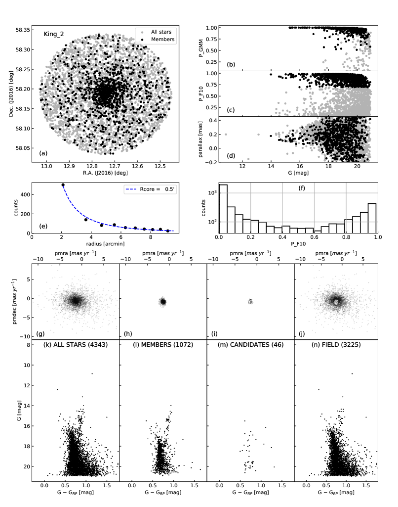
Figure 12: Spatial distribution, VPD and CMDs of King 2. The subplot descriptions are same as Fig. 11.

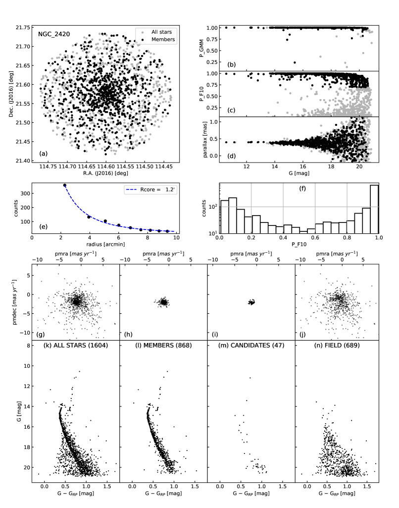
Figure 13: Spatial distribution, VPD and CMDs of NGC 2420. The subplot descriptions are same as Fig. 11.

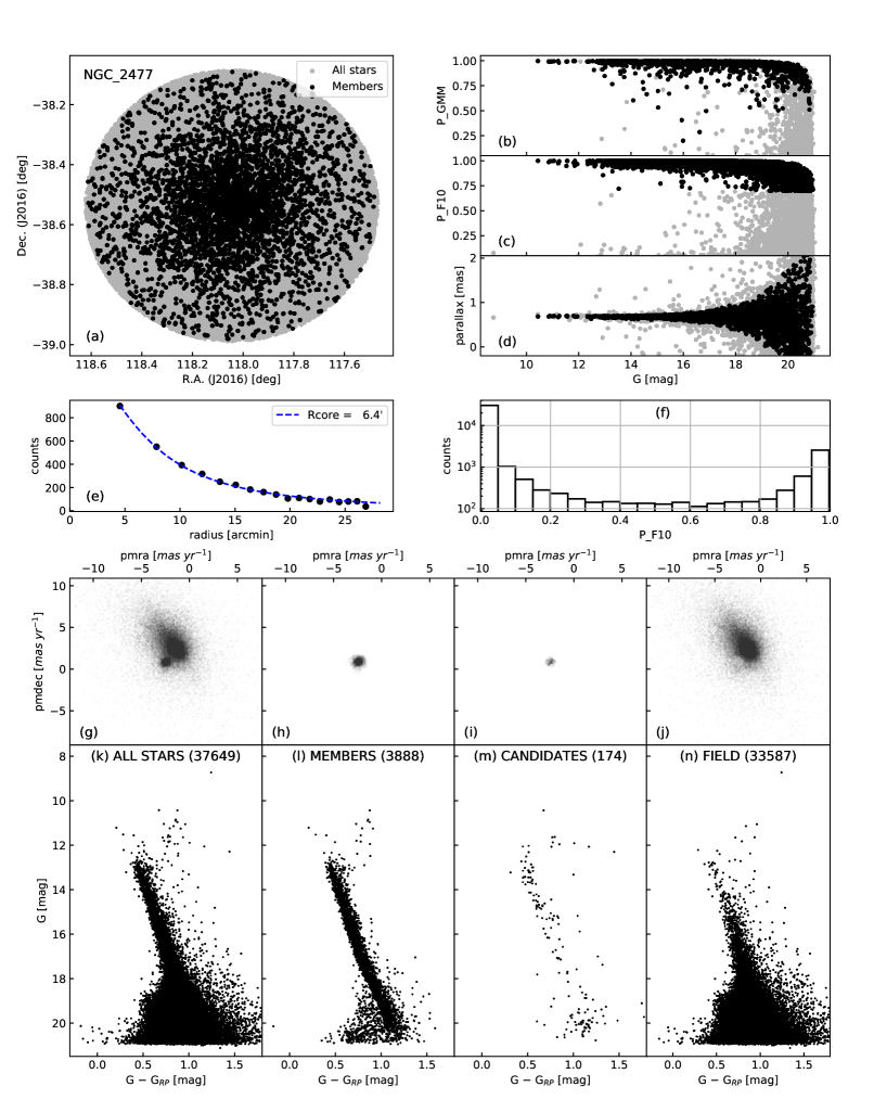
Figure 14: Spatial distribution, VPD and CMDs of NGC 2477. The subplot descriptions are same as Fig. 11.

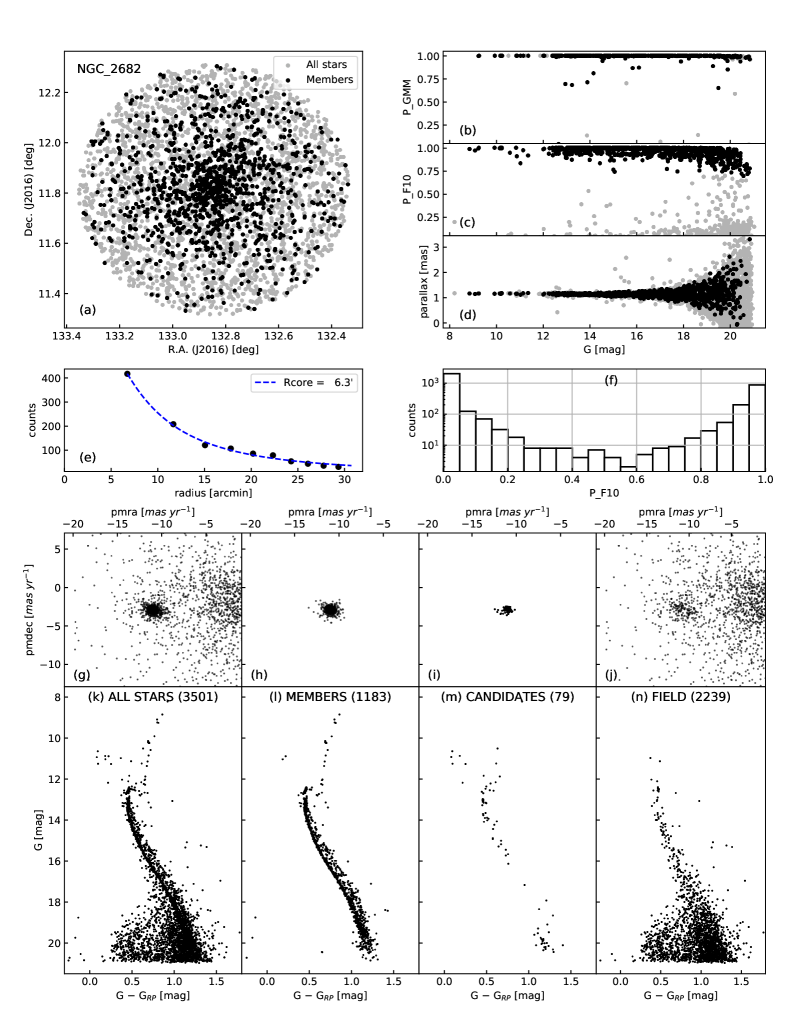
Figure 15: Spatial distribution, VPD and CMDs of NGC 2682. The subplot descriptions are same as Fig. 11.

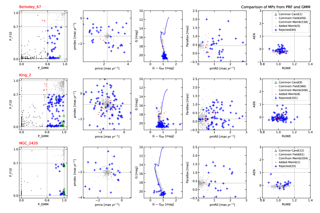
Figure 17: Comparison of MPs from prf and gmm. Common members (P_F10.3 $>$ cutoff and P_GMM) $>$ 0.6) are shown as grey dots, common candidates (P_F10.3 $<$ cutoff and P_F6.4 $>$ cutoff and P_GMM) $>$ 0.6) are shown as green triangles, common field stars (P_F10.3 $<$ cutoff and P_F6.4 $<$ cutoff and P_GMM) $<$ 0.6) are shown as black dots, added members (P_F10.3 $>$ cutoff and P_GMM) $<$ 0.6) are shown as red dots and rejected stars (P_F10.3 $<$ cutoff and P_GMM) $>$ 0.6).

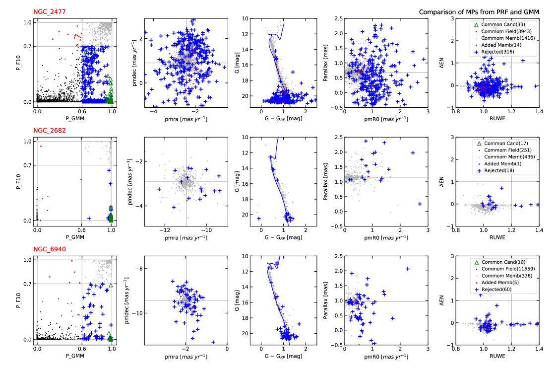
Figure 18: continued

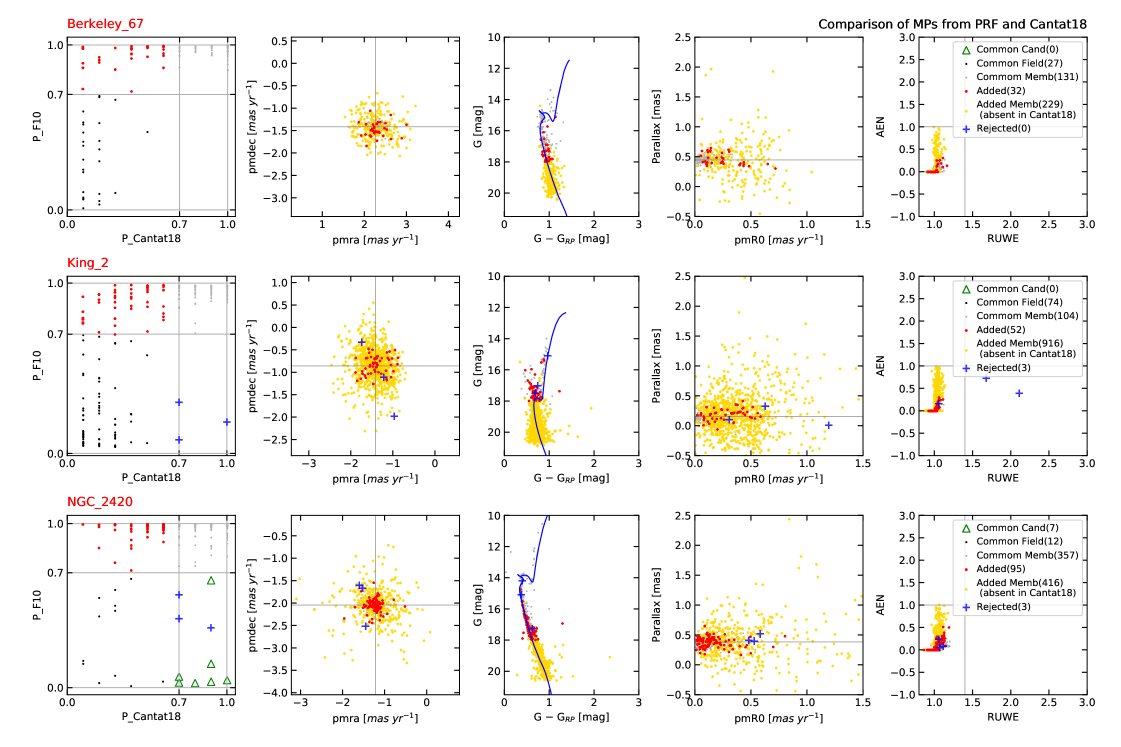
Figure 19: Comparison of MPs from prf and Cantat-Gaudin et al. (2018). The markers for different types of stars and the individual panels are similar to Fig. 17.

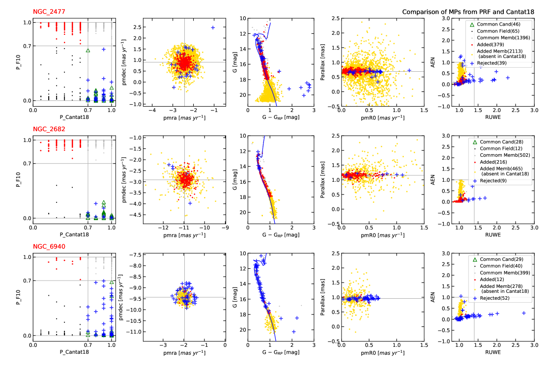
Figure 20: continued

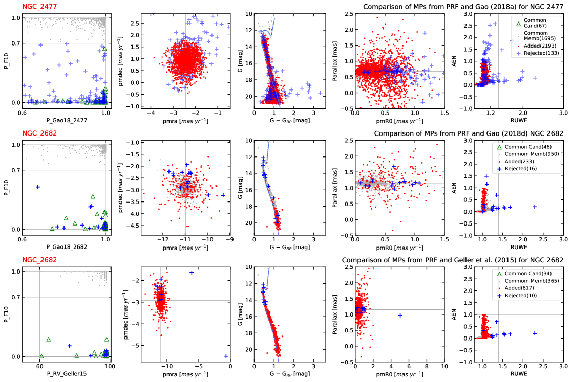
Figure 21: Analysis of membership from prf and Gao (2018a, d) and Geller et al. (2015). The markers for different types of stars and the individual panels are similar to Fig. 17.

References

- Anthony-Twarog et al. (2006) Anthony-Twarog B. J., Tanner D., Cracraft M., Twarog B. A., 2006, AJ, 131, 461
- Aparicio et al. (1990) Aparicio A., Bertelli G., Chiosi C., Garcia-Pelayo J. M., 1990, A&A, 240, 262
- Astropy Collaboration et al. (2013) Astropy Collaboration et al., 2013, A&A, 558, A33
- Balaguer-Nunnez et al. (1998) Balaguer-Nunnez L., Tian K. P., Zhao J. L., 1998, VizieR Online Data Catalog, pp J/A+AS/133/387
- Baratella et al. (2018) Baratella M., Carraro G., D’Orazi V., Semenko E. A., 2018, AJ, 156, 244
- Bellini et al. (2009) Bellini A., et al., 2009, A&A, 493, 959
- Belloni et al. (1998) Belloni T., Verbunt F., Mathieu R. D., 1998, A&A, 339, 431
- Bertelli Motta et al. (2018) Bertelli Motta C., Pasquali A., Caffau E., Grebel E. K., 2018, MNRAS, 480, 4314
- Bonatto et al. (2015) Bonatto C., Campos F., Kepler S. O., Bica E., 2015, MNRAS, 450, 2500
- Bovy Jo et al. (2011) Bovy Jo Hogg D. W., Roweis S. T., 2011, Annals of Applied Statistics, 5, 1657
- Bragaglia et al. (2008) Bragaglia A., Sestito P., Villanova S., Carretta E., Randich S., Tosi M., 2008, A&A, 480, 79
- Bressan et al. (2012) Bressan A., Marigo P., Girardi L., Salasnich B., Dal Cero C., Rubele S., Nanni A., 2012, MNRAS, 427, 127
- Cannon & Lloyd (1970) Cannon R. D., Lloyd C., 1970, MNRAS, 150, 279