Control technique for synchronization of selected nodes in directed networks

Abstract

In this Letter we propose a method to control a set of arbitrary nodes in a directed network such that they follow a synchronous trajectory which is, in general, not shared by the other units of the network. The problem is inspired to those natural or artificial networks whose proper operating conditions are associated to the presence of clusters of synchronous nodes. Our proposed method is based on the introduction of distributed controllers that modify the topology of the connections in order to generate outer symmetries in the nodes to be controlled. An optimization problem for the selection of the controllers, which includes as a special case the minimization of the number of the links added or removed, is also formulated and an algorithm for its solution is introduced.

I Introduction

In the last few decades most of the works on synchronization control in complex networks have focused on the problem of steering the network towards a collective state shared by all the units. Such a synchronized state has been obtained by means of techniques ranging from pinning control [1, 2] to adaptive strategies [3], discontinuous coupling [4], stochastic broadcasting [5] and impulsive control [6]. Other studies have focused on the control of a more structured state where the units split into clusters of synchronized nodes, and each one of these groups follows a different trajectory [7, 8, 9, 10, 11, 12].

In the above mentioned works, the control action is such that all network nodes are forced to follow a given dynamical behavior. However, the number of nodes and links can be very large in real-world systems, so that the question of whether it is possible to control the state of only a subset of the network units, disregarding the behavior of the other units, becomes of great importance. Solving the problem can lead to potentially interesting applications. Consider a team of mobile agents and the case in which a particular task can be accomplished by a subset of the agents only. In such a scenario, one could exploit the relationship between oscillator synchronization and collective motion [13] and apply control techniques for synchronizing a subset of nodes to recruit only a group of all the mobile agents and coordinate them. In a different context, it is well known that synchronization of the whole brain network is associated to pathological states, whereas neural areas are actively synchronized to engage in functional roles [14]. Our approach could provide control techniques supporting neuromorphic engineering applications relying on the principles of neuronal computation [15].

Recently, it has been argued that a subset of network nodes can be controlled by adopting a distributed control paradigm whose formulation relies on the notion of symmetries in a graph [16, 17]. The approach there presented is restricted to undirected graphs, whereas here we propose a control technique for the more general case of directed networks. We find that, in order to form a synchronous cluster, the nodes to control must have the same set of successors, and the common value of their out-degree has to be larger than a threshold, which decreases when the coupling strength in the network is increased. Both conditions can be matched by a proper design of controllers adding to or removing links from the original network structure. The selection of the controllers is addressed by formulating an optimization problem, minimizing an objective function which accounts for the costs associated to adding and/or removing links. We show that an exact solution to the problem can be found, and we propose an algorithm to calculate it.

The rest of the paper is organized as follows: Sec. II contains the preliminaries; the problem is formulated in Sec. III; a theorem illustrating how to design the controllers is illustrated in Sec. IV; the optimization problem and its solution are dealt with in Sec. V; an example of our approach is provided in Sec. VI and the conclusions are drawn in Sec. VII.

II Preliminaries

In this section we introduce notations and definitions used in the rest of the paper [18]. A graph $\mathcal{G}=\left(\mathcal{V},\mathcal{E}\right)$ consists of set of vertices or nodes $\mathcal{V}=\left\{v_{1},...,v_{n}\right\}$ and a set of edges or links $\mathcal{E}\subseteq\mathcal{V}\times\mathcal{V}$. Network nodes are equivalently indicated as $v_{i}$ or, shortly, as $i$. If $\forall\left(v_{i},v_{j}\right)\in\mathcal{E}\Rightarrow\left(v_{j},v_{i}\right)\in\mathcal{E}$, the graph is undirected, otherwise it is directed. Only simple (i.e., containing no loops and no multiple edges) directed graphs are considered in what follows. The set $\mathcal{S}_{i}=\left\{v_{j}\in\mathcal{V}|\left(v_{i},v_{j}\right)\in\mathcal{E}\right\}$ is the set of successors of $v_{i}$ (in undirected graphs $\mathcal{S}_{i}$ coincides with the set of neighbors).

The graph $\mathcal{G}$ can be described through the adjacency matrix $\mathrm{A}$, a $N\times N$ matrix, with $N=|\mathcal{V}|$, and whose elements are $a_{ij}=1$ if $v_{j}\in\mathcal{S}_{i}$ and $a_{ij}=0$, otherwise. We define the out-degree of a node $i$ as the number of its successors, $k_{i}=|\mathcal{S}_{i}|=\sum_{j=1}^{N}a_{ij}$. The Laplacian matrix, $\mathcal{L}$, is defined as $\mathcal{L}=D-\mathrm{A}$, where $D=diag\left\{k_{1},...,k_{N}\right\}$. Its elements are: $\mathcal{L}_{ij}=k_{i}$, if $i=j$, $\mathcal{L}_{ij}=0$, if $i\neq j$ and $v_{j}\notin\mathcal{S}_{i}$, and $\mathcal{L}_{ij}=-1$, if $i\neq j$ and $v_{j}\in\mathcal{S}_{i}$. From the definition it immediately follows that $\mathcal{L}1_{N}=0_{N,1}$ and, so, $0$ is an eigenvalue of the Laplacian matrix with corresponding eigenvector $1_{N}$.

While arguments based on network symmetries are used for controlling groups of nodes in undirected networks [17], directed topologies require the notion of outer symmetrical nodes, here introduced. We define two nodes $v_{i}$ and $v_{j}$ outer symmetrical if $\mathcal{S}_{i}=\mathcal{S}_{j}$ and $\left(v_{i},v_{j}\right)\notin\mathcal{E}$. This notion is more restrictive than that of input equivalence given in [19] for networks including different node dynamics and coupling functions. In [19] the input set of a node $v_{i}$ is defined as $I(v_{i})=\left\{e\in\mathcal{E}:e=\left(v_{i},v_{j}\right)\mbox{ for some }v_{j}\in V\right\}$. Two nodes $v_{i}$ and $v_{j}$ are called input equivalent if and only if there exists a bijection $\beta:I(v_{i})\rightarrow I(v_{j})$ such that the type of connection is preserved, that is the coupling function is the same and the extremes of the edges have the same dynamics. For networks of identical dynamical units and coupling functions, as those considered in our work, input equivalent nodes are nodes with the same out-degree. To be outer symmetrical, a further condition is required: outer symmetrical nodes are input equivalent nodes where the bijection is the identity. This property is fundamental for the control problem dealt with in our paper.

III Problem formulation

Let us consider a directed network of $N$ identical, $n$-dimensional units whose dynamics is given by

$$\dot{x_{i}}=f(x_{i})-\sigma\sum_{j=1}^{N}\mathcal{L}_{ij}\mathrm{H}x_{j}+u_{i},\forall i=1,...,N$$ (1)

with $x_{i}=\left(x_{i1},x_{i2},...,x_{in}\right)^{T}$. Here, $f:\mathbb{R}^{n}\rightarrow\mathbb{R}^{n}$ is the uncoupled dynamics of each unit, $H\in\mathbb{R}^{n\times n}$ is a constant matrix with elements taking values in $\{0,1\}$ that represents inner coupling, i.e., it specifies the components of the state vectors through which node $j$ is coupled to node $i$, and $\sigma>0$ is the coupling strength. $u_{i}$ represent the control actions on the network. Equations (1) with $u_{i}=0$ are extensively used to model diffusively coupled oscillators in biology, chemistry, physics and engineering [20].

Equations (1) can be rewritten in compact form as

$$\dot{\mathbf{x}}=F(\mathbf{x})-\sigma\mathcal{L}\otimes\mathrm{H}\mathbf{x}+\mathbf{u}$$ (2)

where $\mathbf{x}=\left[x_{1}^{T},x_{2}^{T},...,x_{N}^{T}\right]^{T}$, $F(\mathbf{x})=\left[f^{T}(x_{1}),f^{T}(x_{2}),...,f^{T}(x_{N})\right]^{T}$ and $\mathbf{u}=\left[u_{1}^{T},u_{2}^{T},...,u_{N}^{T}\right]^{T}$. In the following we use distributed controllers of the form

$$u_{i}=-\sigma\sum_{j=1}^{N}\mathcal{L}^{\prime}_{ij}\mathrm{H}x_{j}$$ (3)

where $\mathcal{L}^{\prime}$ is a matrix whose elements are $-1$, $0$ or $1$; if $\mathcal{L}_{ij}=0$, setting $\mathcal{L}^{\prime}_{ij}=-1$ introduces a link between two nodes, $i$ and $j$, not connected in the pristine network; on the contrary, setting $\mathcal{L}^{\prime}_{ij}=1$ in correspondence of $\mathcal{L}_{ij}=-1$ removes the existing edge $(v_{i},v_{j})$ in the pristine network; finally, setting $\mathcal{L}^{\prime}_{ij}=0$ indicates no addition or removal of links between $i$ and $j$. The diagonal elements of $\mathcal{L}^{\prime}$ are $\mathcal{L}^{\prime}_{ii}=-\sum_{j=1,j\neq i}^{N}\mathcal{L}^{\prime}_{ij}$. Notice that, even if $\mathcal{L}^{\prime}$ is not a Laplacian, the resulting matrix $\mathcal{L}^{\prime\prime}=\mathcal{L}+\mathcal{L}^{\prime}$ (a matrix representing the network formed by the original topology and the links added or removed by the controllers) is instead a Laplacian.

The system with the controllers reads

$$\dot{\mathbf{x}}=F(\mathbf{x})-\sigma\mathcal{L}^{\prime\prime}\otimes\mathrm{H}\mathbf{x}$$ (4)

The problem tackled in this paper is twofold: i) given an arbitrary subset $V_{n_{2}}$ of $n_{2}<N$ nodes, to determine a set of controllers $u_{i}$ with $i=1,\ldots,N$ such that the nodes in $V_{n_{2}}$ synchronizes to each other; ii) to formulate an optimization problem for the selection of the controllers $u_{i}$.

Without lack of generality, we relabel the network nodes so that the nodes to control are indexed as $i=n_{1}+1,\ldots,N$, such that $V_{n_{2}}=\left\{v_{n_{1}+1},...,v_{N}\right\}$. Objective of the controllers is, therefore, to achieve a synchronous evolution of the type

$$\begin{cases}x_{1}(t)=s_{1}(t)\\ \vdots\\ x_{n_{1}}(t)=s_{n_{1}}(t)\\ x_{n_{1}+1}(t)=x_{n_{1}+2}(t)=...=x_{N}(t)=s(t),\quad t\rightarrow+\infty\end{cases}$$ (5)

In compact form the synchronous state is denoted as $\mathbf{x}^{s}(t)=\left[s_{1}^{T}(t),...,s_{n_{1}}^{T}(t),s^{T}(t),...,s^{T}(t)\right]^{T}$. In the most general case, the trajectories of the first $n_{1}$ nodes are different from each other and from $s(t)$, that is, $s_{i}(t)\neq s_{j}(t)\neq s(t)$ for $i,j=1,\ldots,n_{1}$, but eventually some of them may coincide or converge to $s(t)$. In the next section, we demonstrate how to select the controllers such that the state $\mathbf{x}^{s}(t)$ exists and is locally exponentially stable, while, in the second part of the paper, we consider the optimization problem.

IV Design of the controllers

To achieve a stable synchronous state $\mathbf{x}^{s}(t)$ the controllers $u_{i}$ as in Eq. (3) have to satisfy the conditions expressed by the following theorem.

Theorem IV.1.

Consider the dynamical network (1) and the controllers (3) such that the Laplacian $\mathcal{L}^{\prime\prime}$ satisfies the following conditions:

1. $\mathcal{L}^{\prime\prime}_{i_{1},j}=\mathcal{L}^{\prime\prime}_{i_{2},j}$ for $i_{1}=n_{1}+1,\ldots,N$, $i_{2}=n_{1}+1,\ldots,N$, $j=1,\ldots,N$ and $j\neq i_{1}$, $j\neq i_{2}$;

2. $\mathcal{L}^{\prime\prime}_{i_{1},i_{2}}=0$ for $i_{1}=n_{1}+1,\ldots,N$, $i_{2}=n_{1}+1,\ldots,N$ with $i_{1}\neq i_{2}$;

then, a synchronous behavior $\mathbf{x}^{s}(t)=\left[s_{1}^{T}(t),...,s_{n_{1}}^{T}(t),s^{T}(t),...,s^{T}(t)\right]^{T}$ exists.

In addition, define $k_{i}=\sum_{j}\mathcal{L}^{\prime\prime}_{i,j}$ with $i=n_{1}+1,\ldots,N$, and, since from hypothesis 1) $k_{n_{1}+1}=\ldots=k_{N}$, define $k\triangleq k_{n_{1}+1}=\ldots=k_{N}$. If

1. there exists a diagonal matrix $\mathrm{L}>0$ and two constants $\overline{q}>0$ and $\tau>0$ such that the following linear matrix inequality (LMI) is satisfied $\forall q\geq\overline{q}$ and $t>0$:

   $$\left[Df(s(t))-qH\right]^{T}L+L\left[Df(s(t))-qH\right]\leq-\tau I_{n},$$ (6)

   where $Df(s(t))$ is the Jacobian of $f$ evaluated on $s(t)$;

2. $k$ is such that $k>\frac{\overline{q}}{\sigma}$;

then, the synchronous state is locally exponentially stable.

Proof.

Existence of the synchronous solution. Hypotheses 1) and 2) induce some structural properties in the new network defined by the original topology and the controller links. In particular, hypothesis 1) is equivalent to require that each node in $V_{n_{2}}$ has the same set of successors, that is, $\mathcal{S}^{\prime\prime}_{n_{1}+1}=\ldots=\mathcal{S}^{\prime\prime}_{N}$, while hypothesis 2) requires that there are no links between any pair of nodes in $V_{n_{2}}$, that is, $\forall v_{i},v_{j}\in V_{n_{2}}\Rightarrow\left(v_{i},v_{j}\right)\notin\mathcal{E}$. Consequently, selecting the controllers such that hypotheses 1) and 2) hold makes the nodes in $V_{n_{2}}$ outer symmetrical.

In turns this means that, with reference to the system in Eq. (4), if we permute the nodes in $V_{n_{2}}$, the dynamical network does not change, and the $n_{2}$ nodes have the same equation of motion. If the nodes in $V_{n_{2}}$ start from the same initial conditions, then they remain synchronized for $t>t_{0}$, and thus a synchronous solution $\mathbf{x}^{s}(t)$ as in Eq. (5) exists.

Local exponential stability of the synchronous solution. To prove the stability of $\mathbf{x}^{s}(t)$, we first prove that the synchronous solution $\mathbf{x}^{s}(t)$ is locally exponentially stable if

$$\dot{\zeta}=\left(Df-\sigma kH\right)\zeta$$ (7)

is locally exponentially stable.

We first consider Eq. (4) and linearize it around $\mathbf{x}^{s}(t)$. We define $\eta=\mathbf{x}-\mathbf{x}^{s}$ and calculate its dynamics as

$$\dot{\eta}=DF\eta-\sigma\left(\mathcal{L}^{\prime\prime}\otimes\mathrm{H}\right)\eta$$ (8)

Let us indicate as $Df_{i}$ the Jacobian of $F$ evaluated on $\mathbf{x}^{s}_{i}(t)$. Taking into account Eq. (5), it follows that $Df_{n_{1}+1}=...=Df_{N}\triangleq Df_{s}$ and, hence, $DF=diag\left\{Df_{1},...,Df_{n_{1}},Df_{s},...,Df_{s}\right\}$.

From the structure of $\mathbf{x}^{s}$, it also follows that the synchronous behavior is preserved for all variations belonging to the linear subspace $\mathbb{P}$ generated by the column vectors of the following matrix

$$\mathrm{M}_{s}=\begin{bmatrix}1&0&...&0&0\\ 0&1&...&0&0\\ \vdots&\vdots&\ddots&\vdots&\vdots\\ 0&0&...&1&0\\ 0&0&...&0&\frac{1}{\sqrt{n_{2}}}\\ \vdots&\vdots&\ddots&\vdots&\vdots\\ 0&0&...&0&\frac{1}{\sqrt{n_{2}}}\\ \end{bmatrix}\otimes I_{n}$$

Such variations in fact occur along the synchronization manifold where all the last $n_{2}$ units have the same evolution. The column vectors of $\mathrm{M}_{s}$ represent an orthonormal basis for the considered linear subspace with $dim(\mathbb{P})=n(n_{1}+1)$. The remaining vectors in $\mathbb{R}^{nN}\setminus\mathbb{P}$ represent transversal motions with respect to the synchronization manifold.

An orthonormal basis for $\mathbb{R}^{nN}$ is built by considering a linear vector space $\mathbb{O}$ of $dim(\mathbb{O})=n(n_{2}-1)$ that is orthogonal to $\mathbb{P}$. All vectors of $\mathbb{R}^{nN}$ can be thus expressed as linear combinations of vectors in $\mathbb{P}$ and vectors in $\mathbb{O}$, that is, $\eta=\left(M\otimes I_{n}\right)\xi$ with

$${M}=\begin{bmatrix}1&0&...&0&0&0&...&0\\ 0&1&...&0&0&0&...&0\\ \vdots&\vdots&\ddots&\vdots&\vdots&\vdots&\ddots&\vdots\\ 0&0&...&1&0&0&...&0\\ 0&0&...&0&\frac{1}{\sqrt{n_{2}}}&o_{n_{1}+1,1}&...&o_{n_{1}+1,n_{2}-1}\\ 0&0&...&0&\frac{1}{\sqrt{n_{2}}}&o_{n_{1}+2,1}&...&o_{n_{1}+2,n_{2}-1}\\ \vdots&\vdots&\ddots&\vdots&\vdots&\vdots&\ddots&\vdots\\ 0&0&...&0&\frac{1}{\sqrt{n_{2}}}&o_{N,1}&...&o_{N,n_{2}-1}\\ \end{bmatrix}$$ (9)

For easy of compactness, matrix ${M}$ is rewritten as $M=\begin{bmatrix}I_{n_{1}}&0\\ 0&R_{n_{2}}\\ \end{bmatrix}$.

The evolution of the first $n(n_{1}+1)$ elements of $\xi$ is the evolution of motions along the synchronization manifold, while the remaining elements of $\xi$ are transversal to the synchronization manifold. As a consequence of this, to prove the exponential stability of the synchronization manifold, we have to prove that the evolution of the last $n(n_{2}-1)$ elements of vector $\xi$ decays exponentially to $0$ as $t\rightarrow+\infty$.

We now apply the transformation $\xi=\left(M\otimes I_{n}\right)^{-1}\eta$ to Eqs. (8):

$$\small\begin{array}[]{l}\dot{\xi}=\left(M^{-1}\otimes I_{n}\right)DF\left(M\otimes I_{n}\right)\xi-\sigma\left(M^{-1}\mathcal{L}^{\prime\prime}M\right)\otimes H\xi\end{array}$$ (10)

Straightforward calculations yield that $\left(M^{-1}\otimes I_{n}\right)DF\left(M\otimes I_{n}\right)=DF$. Let us now focus on $M^{-1}\mathcal{L}^{\prime\prime}M$. To calculate this term, we partition $\mathcal{L}^{\prime\prime}$ in (4) as follows:

$$\mathcal{L}^{\prime\prime}=\begin{bmatrix}A_{n_{1}\times n_{1}}&B_{n_{1}\times n_{2}}\\ C_{n_{2}\times n_{1}}&D_{n_{2}\times n_{2}}\\ \end{bmatrix}$$ (11)

From hypothesis 2), it follows that $D=kI_{n_{2}}$. Consider now the block $C_{n_{2}\times n_{1}}$. From hypothesis 1) we have that $\mathcal{L}^{\prime\prime}_{i_{1},j}=\mathcal{L}^{\prime\prime}_{i_{2},j},\forall j\leq n_{1},\forall i_{1},i_{2}>n_{1}$. Denoting with $C_{i}$ the $i$-th row of $C$ we obtain that $C_{i_{1}}=C_{i_{2}},\quad\forall i_{1},i_{2}=1,...,n_{2}$.

Given that

$$\begin{array}[]{c}M^{-1}\mathcal{L}^{\prime\prime}M=\begin{bmatrix}A&BR_{n_{2}}\\ R_{n_{2}}^{T}C&R_{n_{2}}^{T}DR_{n_{2}}\\ \end{bmatrix}\end{array}$$ (12)

since $D=kI_{n_{2}}$ and all the rows in $C$ are equal, we can rewrite $\mathcal{L}^{\prime\prime}$ as:

$$\mathcal{L}^{\prime\prime}=\begin{bmatrix}A&B\\ \begin{matrix}\begin{matrix}c_{1}\\ c_{1}\\ \vdots\\ c_{1}\end{matrix}&...&\begin{matrix}c_{n_{1}}\\ c_{n_{1}}\\ \vdots\\ c_{n_{1}}\end{matrix}\\ \end{matrix}&\begin{matrix}k&0&...&0\\ 0&k&...&0\\ \vdots&\vdots&\ddots&\vdots\\ 0&0&...&k\end{matrix}\end{bmatrix}$$ (13)

where $c_{i}\in\{0,1\}$ if node $i$ is connected or not with the nodes of $V_{n_{2}}$.

Notice that the first row of $R_{n_{2}}^{T}$ is a vector parallel to $\left[1,1,...,1\right]$ while the remaining ones are all orthogonal to it, so:

$$R_{n_{2}}^{T}C=\begin{bmatrix}a_{1}\sqrt{n_{2}}&...&a_{n_{1}}\sqrt{n_{2}}\\ 0&...&0\\ \vdots&\ddots&\vdots\\ 0&...&0\end{bmatrix}$$ (14)

Moreover $R_{n_{2}}^{T}DR_{n_{2}}=R_{n_{2}}^{T}kI_{n_{2}}R_{n_{2}}=kI_{n_{2}}=D$.

It follows that Eq. (10) becomes:

$$\small\begin{array}[]{l}\dot{\xi}=\left[\begin{array}[]{cccc|ccc}Df_{1}&\cdots&0&0&0&\cdots&0\\ \vdots&&\vdots&\vdots&\vdots&&\vdots\\ 0&\cdots&Df_{n_{1}}&0&0&\cdots&0\\ 0&\cdots&0&Df_{s}&0&\cdots&0\\ \hline\cr 0&\cdots&0&0&Df_{s}&\cdots&0\\ \vdots&&\vdots&\vdots&\vdots&&\vdots\\ 0&\cdots&0&0&0&\cdots&Df_{s}\end{array}\right]\xi-\sigma\cdot\\ \left[\begin{array}[]{ccc|cc}l_{11}\ldots&l_{1n_{1}}&l_{1n_{1}+1}&l_{1n_{1}+2}\ldots&l_{1N}\\ \vdots&\vdots&\vdots&\vdots&\vdots\\ l_{n_{1}1}\ldots&l_{n_{1}n_{1}}&l_{n_{1}n_{1}+1}&l_{n_{1}n_{1}+2}\ldots&l_{n_{1}N}\\ c_{1}\sqrt{n_{2}}\ldots&c_{n_{1}}\sqrt{n_{2}}&k&0\ldots&0\\ \hline\cr 0\ldots&0&0&k\ldots&0\\ \vdots&\vdots&\vdots&\vdots&\vdots\\ 0\ldots&0&0&0\ldots&k\end{array}\right]\otimes H\xi\end{array}$$ (15)

where the lines in the matrices suggest a partition highlighting the last $n\left(n_{2}-1\right)$ elements of $\xi$.

The system describing the evolution of variations transversal to the synchronization manifold is uncoupled from the rest of the equations and composed of identical blocks, taking the following form:

$$\dot{\zeta}=\left(Df_{s}-\sigma kH\right)\zeta,\quad\mbox{ with }\zeta\in\mathbb{R}^{n}$$ (16)

It only remains to prove the exponential stability of (16). By hypothesis 4) we have that $k>\frac{\overline{q}}{\sigma}$, thus $k\sigma>\overline{q}$. From the LMI (6) we can use the Lyapunov function $V=\zeta^{T}L\zeta$ to prove exponential stability:

1. $V(0)=0$;

2. $V(\zeta)=\zeta^{T}L\zeta>0,\;\forall\zeta\neq 0$ because $L>0$;

3. $\dot{V}<0,\;\forall\zeta\neq 0$ in fact:

$$\begin{array}[]{l}\frac{d}{dt}\left[\zeta^{T}L\zeta\right]=\dot{\zeta^{T}}L\zeta+\zeta^{T}L\dot{\zeta}\\ =\zeta^{T}\left[\left(Df_{s}-\sigma kH\right)^{T}L+L\left(Df_{s}-\sigma kH\right)\right]\zeta\\ \leq-\tau\zeta^{T}\zeta<0.\end{array}$$ (17)

∎

We note that, in the application of Theorem IV.1, we can first consider the set formed by the union of the successors of the nodes to control. If the cardinality of this set is greater than $\frac{\overline{q}}{\sigma}$, then we can add links such that the successors of each node of $V_{n_{2}}$ are all the elements of this set. Otherwise, one needs to expand this set by including other nodes of the network. Interestingly, the choice of such nodes is totally arbitrary and any node, not yet included in the set of successors, fits for the purpose.

The upper bound of $k$ is the cardinality of $\mathcal{V}\setminus V_{n_{2}}$ and, since Theorem IV.1 requires that $k>\frac{\overline{q}}{\sigma}$, a necessary condition for the application of the proposed technique is that $\sigma>\frac{\overline{q}}{n_{1}}$: if this condition is not met, then, there are not enough nodes in $\mathcal{V}\setminus V_{n_{2}}$ to which the nodes of $V_{n_{2}}$ can be connected by the controllers.

V Optimization

In this section we address the problem of optimizing the controllers with respect to the cost of the links added or removed. Let $w_{ij}^{-}$ ($w_{ij}^{+}$) be the cost associated to the removal of an existing link (addition of a new link) between $i$ and $j$. These parameters account for a general scenario where different links have different costs to change.

Formally, the following minimization problem is considered:

$$\min\limits_{\mathbf{u}\in\mathcal{U}}\sum\limits_{\mathcal{L}^{\prime}_{i,j}=1}\mathcal{L}^{\prime}_{ij}w_{ij}^{-}+\sum\limits_{\mathcal{L}^{\prime}_{i,j}=-1}|\mathcal{L}^{\prime}_{ij}|w_{ij}^{+}$$ (18)

where $\mathcal{U}$ is the set of controllers that satisfies Theorem IV.1 and, thus, ensures the existence and stability of $\mathbf{x}^{s}(t)$. In the special case, when the costs are equal and unitary, i.e., $w_{ij}^{-}=w_{ij}^{+}=1$, the optimization problem reduces to

$$\min\limits_{\mathbf{u}\in\mathcal{U}}\sum\limits_{i,j}|\mathcal{L}^{\prime}_{ij}|$$ (19)

i.e., minimization of the number of links added or removed by the controllers.

Let $\bar{k}\triangleq\lceil\frac{\bar{q}}{\sigma}\rceil$. Theorem IV.1 requires that the nodes in $V_{n_{2}}$ have a number of successors greater than or equal to $\bar{k}$, i.e., since $|\mathcal{S}^{\prime\prime}|=k$, $k\geq\bar{k}$. The optimization problem is thus equivalent to determine the nodes in $\mathcal{S}^{\prime\prime}$ which minimize the objective function (18). Consider the set $\bar{\mathcal{S}}=\bigcup_{v_{i}\in V_{n_{2}}}\mathcal{S}_{i}\setminus V_{n_{2}}$, containing the successors of at least one node of the pristine network that are not in $V_{n_{2}}$. Depending on the cardinality of this set we can have two different scenarios: 1) if $|\bar{\mathcal{S}}|<\overline{k}$, then, ${\mathcal{S}^{\prime\prime}}$ needs to contain all the nodes in $\bar{\mathcal{S}}$ and some other nodes of the set $V_{n_{1}}\setminus\bar{\mathcal{S}}$; 2) if $\left|\bar{\mathcal{S}}\right|\geq\bar{k}$, then, one has to select ${\mathcal{S}^{\prime\prime}}\subset\bar{\mathcal{S}}$. In both cases, the choice of the nodes in ${\mathcal{S}^{\prime\prime}}$ is accomplished taking into account the costs associated to the network links.

First, note that, given $V_{n_{2}}$, to fulfill condition 2) of Theorem IV.1 the links between nodes in this set need to be removed. This yields a fixed cost $\bar{c}=\sum\limits_{i,j\in V_{n_{2}}}a_{ij}w_{ij}^{-}$ such that $\min\limits_{\mathbf{u}\in\mathcal{U}}\sum\limits_{\mathcal{L}^{\prime}_{i,j}=1}\mathcal{L}^{\prime}_{ij}w_{ij}^{-}+\sum\limits_{\mathcal{L}^{\prime}_{i,j}=-1}|\mathcal{L}^{\prime}_{ij}|w_{ij}^{+}\geq\bar{c}$.

Let $c_{i}^{+}$ be the cost to have node $i$ in ${\mathcal{S}^{\prime\prime}}$ and $c_{i}^{-}$ the cost of not including it in ${\mathcal{S}^{\prime\prime}}$. It follows that $c_{i}^{-}=\sum\limits_{j\in V_{n_{2}}}a_{ij}w_{ij}^{-}$ and $c_{i}^{+}=\sum\limits_{j\in V_{n_{2}}}(1-a_{ij})w_{ij}^{+}$. Once calculated $c_{i}^{+}$ and $c_{i}^{-}$, we reformulate the optimization problem in terms of minimization of the overall cost of the control: $Cost=\sum\limits_{v_{i}\in\bar{\mathcal{S}}}\left[c_{i}^{+}x_{i}+c_{i}^{-}(1-x_{i})\right]+\bar{c}$, where $x_{i}$ ($i=1,\ldots,N$) are decisional variables, such that $x_{i}=1$ if $v_{i}\in{\mathcal{S}^{\prime\prime}}$ and $x_{i}=0$ otherwise. The optimization problem now reads:

$$\begin{cases}\min\sum\limits_{v_{i}\in\bar{\mathcal{S}}}\left[c_{i}^{+}x_{i}+c_{i}^{-}(1-x_{i})\right]+\bar{c}\\ \sum\limits_{v_{i}\in\bar{\mathcal{S}}}x_{i}\geq\bar{k}\end{cases}$$ (20)

where the constraint $\sum\limits_{v_{i}\in\bar{\mathcal{S}}}x_{i}\geq\bar{k}$ guarantees that condition $k\geq\bar{k}$ holds. Since the overall cost can be rewritten as $Cost=\sum\limits_{v_{i}\in\bar{\mathcal{S}}}\left(c_{i}^{+}-c_{i}^{-}\right)x_{i}+\sum\limits_{v_{i}\in\bar{\mathcal{S}}}c_{i}^{-}+\bar{c}$ and the terms $\sum\limits_{v_{i}\in\bar{\mathcal{S}}}c_{i}^{-}$ and $\bar{c}$ do not depend on the variables $x_{i}$, the optimization problem becomes

$$\begin{cases}\min\sum\limits_{v_{i}\in\bar{\mathcal{S}}}c_{i}x_{i}\\ \sum\limits_{v_{i}\in\bar{\mathcal{S}}}x_{i}\geq\bar{k}\end{cases}$$ (21)

where $c_{i}\triangleq c_{i}^{+}-c_{i}^{-}$.

This formulation prompts the following solution for the optimization problem. Defining $k^{\prime}\triangleq\left|\left\{v_{i}\in\bar{\mathcal{S}}\;|\;c_{i}\leq 0\right\}\right|$ and sorting the nodes in $\bar{\mathcal{S}}$ in ascending order with respect to their cost $c_{i}$, we take $k_{max}=\max\left\{\bar{k},\;k^{\prime}\right\}$ and assign $x_{i}=1$ to the first $k_{max}$ nodes and $x_{i}=0$ to the remaining ones. The overall cost to achieve synchronization of the nodes in the set $V_{n_{2}}$ is given by

$$Cost=\sum\limits_{v_{i}\in\bar{\mathcal{S}}}c_{i}^{-}+\sum\limits_{v_{i}\in{\mathcal{S}^{\prime\prime}}}c_{i}+\bar{c}$$ (22)

Algorithm 1 is based on the above observations and returns the nodes belonging to ${\mathcal{S}^{\prime\prime}}$. The inputs are $V_{n_{2}}$, $\bar{k}$ and $A$ (the adjacency matrix of the network) and the outputs are the set ${\mathcal{S}^{\prime\prime}}$ and the overall cost.

Algorithm 1 Algorithm to select the nodes in ${\mathcal{S^{\prime\prime}}}$

0:  $V_{n_{2}}$, $\bar{k}$ and $A$

0:  ${\mathcal{S}^{\prime\prime}}$, overall cost $Cost$Initialization:

1:  Create $\bar{\mathcal{S}}=\bigcup_{v_{i}\in V_{n_{2}}}\mathcal{S}_{i}\setminus V_{n_{2}}$ and determine its cardinality $|\bar{\mathcal{S}}|$Procedure:

2:  Calculate $c_{i}^{-}$, $c_{i}^{+}$, $\bar{c}$ and $c_{i}=c_{i}^{+}-c_{i}^{-}$

3:  Sort the nodes in $\bar{\mathcal{S}}$ in ascending order and set $k^{\prime}=\left|\left\{v_{i}\in{\mathcal{S}}\;|\;c_{i}\leq 0\right\}\right|$

4:  Calculate $k_{max}=\max\left\{\bar{k},\;k^{\prime}\right\}$

5:  if $|\bar{\mathcal{S}}|\geq\bar{k}$ then

6:     return  $Cost=\bar{c}+\sum\limits_{v_{i}\in\bar{\mathcal{S}}}c_{i}^{-}+\sum\limits_{v_{i}\in\bar{\mathcal{S}^{\prime\prime}}}c_{i}$ and build ${\mathcal{S}^{\prime\prime}}$ taking the first $k_{max}$ nodes in $\bar{\mathcal{S}}$

7:  else

8:     Build ${\mathcal{S}^{\prime\prime}}$ taking all the elements of $\bar{\mathcal{S}}$ and add nodes from $V_{n_{1}}\setminus\bar{\mathcal{S}}$, in ascending order of $c_{i}$, until $|{\mathcal{S^{\prime\prime}}}|=\bar{k}$

9:  end if

10:  return  $Cost$ and ${\mathcal{S}^{\prime\prime}}$

VI Examples

We now discuss an example of how the proposed control works in the directed network with $N=20$ nodes shown in Fig. 1. We refer to several cases, corresponding to two distinct sets of nodes to control, $V_{n_{2}}$, two values of $\bar{k}$, and different costs associated to the links. For each of these cases, the controllers that satisfy Theorem IV.1 and are the result of the optimization procedure of Sec. V are discussed; we will show that they depend on the control goal, on the link costs and, through $\bar{k}$, on the coupling coefficient.

More specifically, we first consider unitary costs for the links and synchronization of two different triplets of nodes, i.e., either $V_{n_{2}}=\{1,4,16\}$ or $V_{n_{2}}=\{1,3,19\}$, with two values of $\bar{k}$, i.e., $\bar{k}=1$ and $\bar{k}=3$. This leads to cases 1-4 in Table I. Case 5, instead, refers to a scenario where the costs are not unitary.

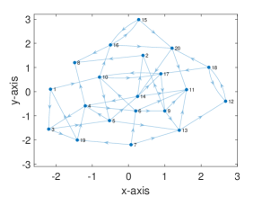
Figure 1: Case study: a directed network of $N=20$ nodes. The spatial position of the network nodes is used to define costs for link addition proportional to the Euclidean distance of the nodes to be connected.

Case 1: $V_{n_{2}}=\{1,4,16\}$, $\bar{k}=1$. Here, we have that $\bar{\mathcal{S}}=\{3,6,8,10,15,20\}$ and $|\bar{\mathcal{S}}|>\bar{k}$. Following Algorithm 1, we find $k^{\prime}=2$, so that $k^{\prime}>\bar{k}$ and ${\mathcal{S}^{\prime\prime}}=\{3,8\}$. Synchronization of the nodes in $V_{n_{2}}$ is achieved if two links are added to the original network, and four links are removed.

Case 2: $V_{n_{2}}=\{1,4,16\}$, $\bar{k}=3$. Here again $|\bar{\mathcal{S}}|>\bar{k}$, but $k^{\prime}<\bar{k}$. We get ${\mathcal{S}^{\prime\prime}}=\{3,6,8\}$, four links to add and three to remove.

Case 3: $V_{n_{2}}=\{1,3,19\}$, $\bar{k}=1$. We have $\bar{\mathcal{S}}=\{4,10\}$ and $|\bar{\mathcal{S}}|>\bar{k}$. In this case, we obtain ${\mathcal{S}^{\prime\prime}}=\{4\}$, a single link to add and three links to remove.

Case 4: $V_{n_{2}}=\{1,3,19\}$, $\bar{k}=3$. We have $\left|\bar{\mathcal{S}}\right|<\bar{k}$ thus, following step 8 of the algorithm, we need to add a node from $V_{n_{1}}\setminus\bar{\mathcal{S}}$, i.e. a node which is not a successor of any of the nodes to be synchronized. As the choice is completely arbitrary, we select node $6$. So, ${\mathcal{S}^{\prime\prime}}=\{4,6,10\}$. Control is attained by adding seven links and removing three links.

Case 5: $V_{n_{2}}=\{1,4,16\}$, $\bar{k}=3$, non-unitary costs. For the purpose of illustration, here we assume that the cost to add a link is proportional to the distance between the two nodes, while removing links always has a unitary cost. We consider the synchronization problem as in case 2. Here, the different costs yield a different result for ${\mathcal{S}^{\prime\prime}}$, i.e., ${\mathcal{S}^{\prime\prime}}=\{3,8,10\}$. In this scenario, optimization requires to include in ${\mathcal{S}^{\prime\prime}}$ node 10 rather than node 6.

TABLE I: Added and removed links obtained for different $V_{n_{2}}$ and $\bar{k}$ for the network in Fig. 1. Costs associated to links are considered unitary in all cases, except for case 5.

Case	$V_{n_{2}}$	$\bar{k}$	Added links	Removed links
1	{1,4,16}	1	(1,8) (16,3)	(16,15) (16,20) (1,10) (4,6)
2	{1,4,16}	3	(1,8) (16,3) (1,6) (16,6)	(16,15) (16,20) (1,10)
3	{1,3,19}	1	(1,4)	(1,10) (1,3) (19,1)
4	{1,3,19}	3	(1,6) (1,4) (3,10) (3,4) (3,6) (19,20) (19,6)	(19,1) (1,3) (3,19)
5*	{1,4,16}	3	(1,8) (4,10) (16,3) (16,10)	(4,6) (16,15) (16,20)

Finally, for case 2 we report the waveforms obtained by simulating the network with control (Fig. 2). Chua’s circuits starting from random initial conditions are considered (equations and parameters have been fixed as in [17]). Fig. 2 shows that the nodes in $V_{n_{2}}=\{1,4,16\}$ follow the same trajectory, while the remaining units are not synchronized with them. Similar results are obtained for the other scenarios.

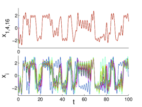
Figure 2: Evolution of the first state variable for nodes in $V_{n_{2}}=\{1,4,16\}$ (upper plot) and for all the network nodes (bottom plot).

VII Conclusions

In this work we have focused on the problem of controlling synchronization of a group of nodes in directed networks. The nodes are all assumed to have the same dynamics and, similarly, coupling is assumed to be fixed to the same value along all the links of the network. The technique we propose is based on the use of distributed controllers which add further links to the network or remove some of the existing ones, creating a new network structure which has to satisfy two topological conditions. The first condition refers to the fact that, in the new network, merging the existing links and those of the controllers, the nodes to control must be outer symmetrical, while the second condition requires that the out-degree of these nodes has to be higher than a threshold. Quite interestingly, the threshold depends on the dynamics of the units and on the coupling strength, in such a way that a higher coupling strength favors control as it requires a smaller out-degree. It is also worth noticing that, when the out-degree needs to be increased to exceed the threshold, this can be obtained by connecting to any of the remaining nodes of the network.

The selection of the nodes forming the set of successors of the units to control is carried out by considering an optimization problem and finding the exact solution that minimizes the cost of the changes (i.e. link additions or removals). In the case of unitary costs, the problem reduces to minimization of the number of added or removed links, thereby defining a strategy for the control of synchronization of a group of nodes in a directed network with minimal topological changes.

References

• [1] T. Chen, X. Liu, and W. Lu, “Pinning complex networks by a single controller,” IEEE Trans. on Circ. Sys. I, vol. 54, no. 6, pp. 1317–1326, 2007.
• [2] W. Yu, G. Chen, and J. Lü, “On pinning synchronization of complex dynamical networks,” Automatica, vol. 45, no. 2, pp. 429–435, 2009.
• [3] P. DeLellis, F. Garofalo et al., “Novel decentralized adaptive strategies for the synchronization of complex networks,” Automatica, vol. 45, no. 5, pp. 1312–1318, 2009.
• [4] M. Coraggio, P. De Lellis, S. J. Hogan, and M. di Bernardo, “Synchronization of networks of piecewise-smooth systems,” IEEE Control Systems Letters, 2018.
• [5] R. Jeter, M. Porfiri, and I. Belykh, “Network synchronization through stochastic broadcasting,” IEEE Control Systems Letters, vol. 2, no. 1, pp. 103–108, 2018.
• [6] Z.-H. Guan, Z.-W. Liu, G. Feng, and Y.-W. Wang, “Synchronization of complex dynamical networks with time-varying delays via impulsive distributed control,” IEEE Trans. Circ. Sys. I, vol. 57, no. 8, pp. 2182–2195, 2010.
• [7] W. Wu, W. Zhou, and T. Chen, “Cluster synchronization of linearly coupled complex networks under pinning control,” IEEE Trans. Circ. Syst. I, vol. 56, no. 4, pp. 829–839, 2009.
• [8] H. Su, Z. Rong, M. Z. Chen, X. Wang, G. Chen, and H. Wang, “Decentralized adaptive pinning control for cluster synchronization of complex dynamical networks,” IEEE Transactions on Cybernetics, vol. 43, no. 1, pp. 394–399, 2013.
• [9] Q. Ma and J. Lu, “Cluster synchronization for directed complex dynamical networks via pinning control,” Neurocomputing, vol. 101, pp. 354–360, 2013.
• [10] C. B. Yu, J. Qin, and H. Gao, “Cluster synchronization in directed networks of partial-state coupled linear systems under pinning control,” Automatica, vol. 50, no. 9, pp. 2341–2349, 2014.
• [11] L. V. Gambuzza and M. Frasca, “A criterion for stability of cluster synchronization in networks with external equitable partitions,” Automatica, vol. 100, pp. 212–218, 2019.
• [12] T. H. Lee, Q. Ma, S. Xu, and J. H. Park, “Pinning control for cluster synchronisation of complex dynamical networks with semi-markovian jump topology,” Int. J. Control, vol. 88, no. 6, pp. 1223–1235, 2015.
• [13] D. A. Paley, N. E. Leonard, R. Sepulchre, D. Grunbaum, and J. K. Parrish, “Oscillator models and collective motion,” IEEE Control Systems Magazine, vol. 27, no. 4, pp. 89–105, 2007.
• [14] R. T. Canolty, K. Ganguly, S. W. Kennerley, C. F. Cadieu, K. Koepsell, J. D. Wallis, and J. M. Carmena, “Oscillatory phase coupling coordinates anatomically dispersed functional cell assemblies,” Proceedings of the National Academy of Sciences, vol. 107, no. 40, pp. 17 356–17 361, 2010.
• [15] G. Indiveri and T. K. Horiuchi, “Frontiers in neuromorphic engineering,” Frontiers in neuroscience, vol. 5, p. 118, 2011.
• [16] V. Nicosia, M. Valencia, M. Chavez, A. Díaz-Guilera, and V. Latora, “Remote synchronization reveals network symmetries and functional modules,” Phys. Rev. Lett., vol. 110, p. 174102, 2013.
• [17] L. V. Gambuzza, M. Frasca, and V. Latora, “Distributed control of synchronization of a group of network nodes,” IEEE Trans. Automatic Control, vol. 64, no. 1, pp. 362–369, 2019.
• [18] V. Latora, V. Nicosia, and G. Russo, Complex networks: principles, methods and applications.   Cambridge University Press, 2017.
• [19] M. Golubitsky and I. Stewart, “Nonlinear dynamics of networks: the groupoid formalism,” Bulletin of the American Mathematical Society, vol. 43, no. 3, pp. 305–364, 2006.
• [20] A. Arenas, A. Díaz-Guilera, J. Kurths, Y. Moreno, and C. Zhou, “Synchronization in complex networks,” Physics Reports, vol. 469, no. 3, pp. 93–153, 2008.