$\mathsf{SPRISS}$: Approximating Frequent $k$-mers by Sampling Reads,
and Applications

Abstract

The extraction of $k$-mers is a fundamental component in many complex analyses of large next-generation sequencing datasets, including reads classification in genomics and the characterization of RNA-seq datasets. The extraction of all $k$-mers and their frequencies is extremely demanding in terms of running time and memory, owing to the size of the data and to the exponential number of $k$-mers to be considered. However, in several applications, only frequent $k$-mers, which are $k$-mers appearing in a relatively high proportion of the data, are required by the analysis. In this work we present $\mathsf{SPRISS}$, a new efficient algorithm to approximate frequent $k$-mers and their frequencies in next-generation sequencing data. $\mathsf{SPRISS}$ employs a simple yet powerful reads sampling scheme, which allows to extract a representative subset of the dataset that can be used, in combination with any $k$-mer counting algorithm, to perform downstream analyses in a fraction of the time required by the analysis of the whole data, while obtaining comparable answers. Our extensive experimental evaluation demonstrates the efficiency and accuracy of $\mathsf{SPRISS}$ in approximating frequent $k$-mers, and shows that it can be used in various scenarios, such as the comparison of metagenomic datasets and the identification of discriminative $k$-mers, to extract insights in a fraction of the time required by the analysis of the whole dataset.

keywords: $k$-mer analysis; frequent $k$-mers; read sampling; pseudodimension;

1 Introduction

The study of substrings of length $k$, or $k$-mers, is a fundamental task in the analysis of large next-generation sequencing datasets. The extraction of $k$-mers, and of the frequencies with which they appear in a dataset of reads, is a crucial step in several applications, including the comparison of datasets and reads classification in metagenomics [59], the characterization of variation in RNA-seq data [3], the analysis of structural changes in genomes [22, 23], RNA-seq quantification [40, 62], fast search-by-sequence over large high-throughput sequencing repositories [53], genome comparison [51], and error correction for genome assembly [19, 50].

$k$-mers and their frequencies can be obtained with a linear scan of a dataset. However, due to the massive size of the modern datasets and the exponential growth of the $k$-mers number (with respect to $k$), the extraction of $k$-mers is an extremely computationally intensive task, both in terms of running time and memory [13], and several algorithms have been proposed to reduce the running time and memory requirements (see Section 1.2). Nonetheless, the extraction of all $k$-mers and their frequencies from a reads dataset is still highly demanding in terms of time and memory (e.g., KMC 3 [20], one of the currently best performing tools for $k$-mer counting, requires more than $2.5$ hours, $34$ GB of memory, and $500$ GB of space on disk on a sequence of $729$ Gbases [20], and from our experiments more than $30$ minutes, $300$ GB of memory, and $97$ GB of disk space for counting $k$-mers from Mo17 dataset).

While some applications, such as error correction  [19, 50] or reads classification [59], require to identify all $k$-mers, even the ones that appear only once or few times in a dataset, other analyses, such as the comparison of abundances in metagenomic datasets [4, 11, 12, 41] or the discovery of $k$-mers discriminating between two datasets [37, 23], hinge on the identification of frequent $k$-mers, which are $k$-mers appearing with a (relatively) high frequency in a dataset. For the latter analyses, tools capable of efficiently extracting frequent $k$-mers only would be extremely beneficial and much more efficient than tools reporting all $k$-mers (given that a large fraction of $k$-mers appear with extremely low frequency). However, the efficient identification of frequent $k$-mers and their frequencies is still relatively unexplored (see Section 1.2).

A natural approach to speed-up the identification of frequent $k$-mers is to analyze only a sample of the data, since frequent $k$-mers appear with high probability in a sample, while unfrequent $k$-mers appear with lower probability. A major challenge in sampling approaches is how to rigorously relate the results obtained analyzing the sample and the results that would be obtained analyzing the whole dataset. Tackling such challenge requires to identify a minimum sample size which guarantees that the results on the sample well represent the results to be obtained on the whole dataset. An additional challenge in the use of sampling for the identification of frequent $k$-mers is due to the fact that, for values of $k$ of interest in modern applications (e.g., $k\in[20,60]$), even the most frequent $k$-mers appear in a relatively low portion of the data (e.g., $10^{-7}\text{-}10^{-5}$). The net effect is that the application of standard sampling techniques to rigorously approximate frequent $k$-mers results in sample sizes larger than the initial dataset.

1.1 Our Contributions

In this work we study the problem of approximating frequent $k$-mers in a dataset of reads. In this regard, our contributions are:

• We propose $\mathsf{SPRISS}$, SamPling Reads algorIthm to eStimate frequent $k$-merS. $\mathsf{SPRISS}$ is based on a simple yet powerful read sampling approach, which renders $\mathsf{SPRISS}$ very flexible and suitable to be used in combination with any $k$-mer counter. In fact, the read sampling scheme of $\mathsf{SPRISS}$ returns a representative subset of a dataset of reads, which can be used to obtain representative results for down-stream analyses based on frequent $k$-mers.

• We prove that $\mathsf{SPRISS}$ provides rigorous guarantees on the quality of the approximation of the frequent $k$-mers. In this regard, our main technical contribution is the derivation of the sample size required by $\mathsf{SPRISS}$, obtained through the study of the pseudodimension [42], a key concept from statistical learning theory, of $k$-mers in reads.

• We show on several real datasets that $\mathsf{SPRISS}$ approximates frequent $k$-mers with high accuracy, while requiring a fraction of the time needed by approaches that analyze all $k$-mers in a dataset.

• We show the benefits of using the approximation of frequent $k$-mers obtained by $\mathsf{SPRISS}$ in two applications: the comparison of metagenomic datasets, and the extraction of discriminative $k$-mers. In both applications $\mathsf{SPRISS}$ significantly speeds up the analysis, while providing the same insights obtained by the analysis of the whole data.

1.2 Related Works

The problem of exactly counting $k$-mers in datasets has been extensively studied, with several methods proposed for its solution [21, 26, 32, 46, 2, 47, 20, 39]. Such methods are typically highly demanding in terms of time and memory when analyzing large high-throughput sequencing datasets [13]. For this reason, many methods have been recently developed to compute approximations of the $k$-mers abundances to reduce the computational cost of the task (e.g, [31, 52, 34, 8, 61, 39]). However, such methods do not provide guarantees on the accuracy of their approximations that are simultaneously valid for all (or the most frequent) $k$-mers. In recent years other problems closely related to the task of counting $k$-mers have been studied, including how to efficiently index [38, 15, 30, 28], represent [7, 10, 1, 14, 14, 29, 17, 44], query [53, 54, 60, 55, 5, 27], and store [18, 35, 16, 43] the massive collections of sequences or of $k$-mers that are extracted from the data.

A natural approach to reduce computational demands is to analyze a small sample instead of the entire dataset. To this end, methods that perform a downsampling of massive datasets have been recently proposed [6, 58, 9]. These methods focus on discarding reads of the datasets that are very similar to the reads already included in the sample, computing approximate similarity measures as each read is considered. Such measures (i.e., the Jaccard similarity) are designed to maximise the diversity of the content of the reads in the sample. This approach is well suited for applications where rare $k$-mers are important, but they are less relevant for analyses, of interest to this work, where the most frequent $k$-mers carry the major part of the information. Furthermore, these methods have a heuristic nature, and do not provide guarantees on the relation between the accuracy of the analysis performed on the sample w.r.t. the analysis performed on the entire dataset. SAKEIMA [41] is the first sampling method that provides an approximation of the set of frequent $k$-mers (together with their estimated frequencies) with rigorous guarantees, based on counting only a subset of all occurrences of $k$-mers, chosen at random. SAKEIMA performs a full scan of the entire dataset, in a streaming fashion, and processes each $k$-mer occurence according to the outcome of its random choices. $\mathsf{SPRISS}$, the algorithm we present in this work, is instead the first sampling algorithm to approximate frequent $k$-mers (and their frequencies), with rigorous guarantees, by sampling reads from the dataset. In fact, $\mathsf{SPRISS}$ does not require to receive in input and to scan the entire dataset, but, instead, it needs in input only a small sample of reads drawn from the dataset, sample that may be obtained, for example, at the time of the physical creation of the whole dataset. While the sampling strategy of SAKEIMA could be analyzed using the concept of VC dimension [57], the reads-sampling strategy of $\mathsf{SPRISS}$ requires the more sophisticated concept of pseudodimension [42], for its analysis.

In this work we consider the use of $\mathsf{SPRISS}$ to speed up the computation of the Bray-Curtis distance between metagenomic datatasets and the identification of discriminative $k$-mers. Computational tools for these problems have been recently proposed [4, 49]. These tools are based on exact $k$-mer counting strategies, and the approach we propose with $\mathsf{SPRISS}$ could be applied to such strategies as well.

2 Preliminaries

Let $\Sigma$ be an alphabet of $\sigma$ symbols. A dataset $\mathcal{D}=\{r_{1},\dots,r_{n}\}$ is a bag of $|\mathcal{D}|=n$ reads, where, for $i\in\{1,\dots,n\}$, a read $r_{i}$ is a string of length $n_{i}$ built from $\Sigma$. For a given integer $k$, a $k$-mer $K$ is a string of length $k$ on $\Sigma$, that is $K\in\Sigma^{k}$. Given a $k$-mer $K$, a read $r_{i}$ of $\mathcal{D}$, and a position $j\in\{0,\dots,n_{i}-k\}$, we define the indicator function $\phi_{r_{i},K}(j)$ to be $1$ if $K$ appears in $r_{i}$ at position $j$, that is $K[h]=r_{i}[j+h]$ $\forall h\in\{0,\dots,k-1\}$, while $\phi_{r_{i},K}(j)$ is $0$ otherwise. The size $t_{\mathcal{D},k}$ of the multiset of $k$-mers that appear in $\mathcal{D}$ is $t_{\mathcal{D},k}=\sum_{r_{i}\in\mathcal{D}}(n_{i}-k+1)$. The average size of the multiset of $k$-mers that appear in a read of $\mathcal{D}$ is $\ell_{\mathcal{D},k}=t_{\mathcal{D},k}/n$, while the maximum value of such quantity is $\ell_{\max,\mathcal{D},k}=\max_{r_{i}\in\mathcal{D}}(n_{i}-k+1)$. The support $o_{\mathcal{D}}(K)$ of $k$-mer $K$ in dataset $\mathcal{D}$ is the number of distinct positions of $\mathcal{D}$ where $k$-mer $K$ appears, that is $o_{\mathcal{D}}(K)=\sum_{r_{i}\in\mathcal{D}}\sum_{j=0}^{n_{i}-k}\phi_{r_{i},K}(j)$. The frequency $f_{\mathcal{D}}(K)$ of a $k$-mer $K$ in $\mathcal{D}$ is the fraction of all positions in $\mathcal{D}$ where $K$ appears, that is $f_{\mathcal{D}}(K)=o_{\mathcal{D}}(K)/t_{\mathcal{D},k}$.

The task of finding frequent $k$-mers (FKs) is defined as follows: given a dataset $\mathcal{D}$, a positive integer $k$, and a minimum frequency threshold $\theta\in(0,1]$, find the set $FK(\mathcal{D},k,\theta)$ of all the $k$-mers whose frequency in $\mathcal{D}$ is at least $\theta$, and their frequencies, that is $FK(\mathcal{D},k,\theta)=\{(K,f_{\mathcal{D}}(K)):K\in\Sigma^{k},f_{\mathcal{D}}(K)\geq\theta\}$.

The set of frequent $k$-mers can be computed by scanning the dataset and counting the number of occurrences for each $k$-mers. However, when dealing with a massive dataset $\mathcal{D}$, the exact computation of the set $FK(\mathcal{D},k,\theta)$ requires large amount of time and memory. For this reason, one could instead focus on finding an approximation of $FK(\mathcal{D},k,\theta)$ with rigorous guarantees on its quality. In this work we consider the following approximation, introduced in [41].

Definition 1.

Given a dataset $\mathcal{D}$, a positive integer $k$, a frequency threshold $\theta\in(0,1]$, and an accuracy parameter $\varepsilon\in(0,\theta)$, an $\varepsilon$-approximation $\mathcal{C}=\{(K,f_{K}):K\in\Sigma^{k},f_{K}\in[0,1]\}$ of $FK(\mathcal{D},k,\theta)$ is a set of pairs $(K,f_{K})$ with the following properties:

• $\mathcal{C}$ contains a pair $(K,f_{K})$ for every $(K,f_{\mathcal{D}}(K))\in FK(\mathcal{D},k,\theta)$;

• $\mathcal{C}$ contains no pair $(K,f_{K})$ such that $f_{\mathcal{D}}(K)<\theta-\varepsilon$;

• for every $(K,f_{K})\in\mathcal{C}$, it holds $|f_{\mathcal{D}}(K)-f_{K}|\leq\varepsilon/2$.

Intuitively, the approximation $\mathcal{C}$ contains no false negatives (i.e. all the frequent $k$-mers in $FK(\mathcal{D},k,\theta)$ are in $C$) and no $k$-mer whose frequency in $\mathcal{D}$ is much smaller than $\theta$. In addition, the frequencies in $\mathcal{C}$ are good approximations of the actual frequencies in $\mathcal{D}$, i.e. within a small error $\varepsilon/2$.

Definition 2.

Given a dataset $\mathcal{D}$ of $n$ reads, we define a reads sample $S$ of $\mathcal{D}$ as a bag of $m$ reads, sampled independently and uniformly at random, with replacement, from the bag of reads in $\mathcal{D}$.

A natural way to compute an approximation of the set of frequent $k$-mers is by processing a sample, i.e. a small portion of the dataset $\mathcal{D}$, instead of the whole dataset. While previous work [41] considered samples obtained by drawing $k$-mers independently from $\mathcal{D}$, we consider samples obtained by drawing entire reads. As explained in Section 1.1, our approach has several advantages, including the fact that it can be combined with any efficient $k$-mer counting procedure, and that it can be used to extract a representative subset of the data on which to conduct down-stream analyses obtaining, in a fraction of the time required to process the whole dataset, the same insights. Such representative subsets could be stored and used for exploratory analyses, with a gain in terms of space and time requirements compared to using the whole dataset.

However, the development of an efficient scheme to effectively approximate the frequency of all frequent $k$-mers by sampling reads is highly nontrivial, due to dependencies among $k$-mers appearing in the same read. In the next sections, we develop and analyze algorithms to approximate $FK(\mathcal{D},k,\theta)$ by read sampling, starting from a straightforward, but inefficient, approach (Section 3), then showing how pseudodimension can be used to improve the sample size required by such approach (Section 4), and culminating in our algorithm $\mathsf{SPRISS}$, the first efficient algorithm to approximate frequent $k$-mers by read sampling (Section 5).

3 Warm-Up: A Simple Algorithm for Approximating Frequent $k$-mers by Sampling Reads

A first, simple approach to approximate the set $FK(\mathcal{D},k,\theta)$ of frequent $k$-mers consists in taking a sample $S$ of $m$ reads, with $m$ large enough, and report in output the set $FK(S,k,\theta-\varepsilon/2)$ of $k$-mers that appear with frequency at least $\theta-\varepsilon/2$ in the sample $S$. The following result, obtained by combining Hoeffding’s inequality [33] and a union bound, provides an upper bound to the number $m$ of reads required to have guarantees on the quality of the approximation (see Supplement Material Section A for the full analysis).

Proposition 1.

Consider a sample $S$ of $m$ reads from $\mathcal{D}$. For fixed frequency threshold $\theta\in(0,1]$, error parameter $\varepsilon\in(0,\theta)$, and confidence parameter $\delta\in(0,1)$, if $m\geq\frac{2}{\varepsilon^{2}}\left(\frac{\ell_{\max,\mathcal{D},k}}{\ell_{\mathcal{D},k}}\right)^{2}\left(\ln\left(2\sigma^{k}\right)+\ln\left(\frac{1}{\delta}\right)\right)$ then, with probability $\geq 1-\delta$, $FK(S,k,\theta-\varepsilon/2)$ is an $\varepsilon$-approximation of $FK(\mathcal{D},k,\theta)$.

While the result above provides a first bound to the number $m$ of reads required to obtain a rigorous approximation of the frequent $k$-mers, it usually results in a sample size $m$ larger than $|\mathcal{D}|$ (this is due to the need for $\varepsilon$ to be small in order to obtain meaningful approximations, see Section 6.2), making the sampling approach useless. Thus, in the next sections we propose advanced methods to reduce the sample size $m$.

4 A First Improvement: A Pseudodimension-based Algorithm for $k$-mers Approximation by Sampling Reads

In this section we introduce the notion of pseudodimension and we use it to improve the bound on the sample size $m$ of Proposition 1.

Let $\mathcal{F}$ be a class of real-valued functions from a domain $X$ to $[a,b]\subset\mathbb{R}$. Consider, for each $f\in\mathcal{F}$, the subset of $X^{\prime}=X\times[a,b]$ defined as $R_{f}=\{(x,t):t\leq f(x)\}$, and call it range. Let $\mathcal{F}^{+}=\{R_{f},f\in\mathcal{F}\}$ be a range set on $X^{\prime}$, and its corresponding range space $Q^{\prime}$ be $Q^{\prime}=(X^{\prime},\mathcal{F}^{+})$. We say that a subset $D\subset X^{\prime}$ is shattered by $\mathcal{F}^{+}$ if the size of the projection set $proj_{\mathcal{F}^{+}}(D)=\{r\cap D:r\in\mathcal{F}^{+}\}$ is equal to $2^{|D|}$. The VC dimension $VC(Q^{\prime})$ of $Q^{\prime}$ is the maximum size of a subset of $X^{\prime}$ shattered by $\mathcal{F}^{+}$. The pseudodimension $PD(X,\mathcal{F})$ is then defined as the VC dimension of $Q^{\prime}$: $PD(X,\mathcal{F})=VC(Q^{\prime})$.

Let $\pi$ be the uniform distribution on $X$, and let $S$ be a sample of $X$ of size $|S|=m$, with every element of $S$ sampled independently and uniformly at random from $X$. We define, $\forall f\in\mathcal{F}$, $f_{S}=\frac{1}{m}\sum_{x\in S}f(x)$ and $f_{X}=\mathbb{E}_{x\sim\pi}[f(x)]$. Note that $\mathbb{E}[f_{S}]=f_{X}$. The following result relates the accuracy and confidence parameters $\varepsilon$,$\delta$ and the pseudodimension with the probability that the expected values of the functions in $\mathcal{F}$ are well approximated by their averages computed from a finite random sample.

Proposition 2 ([56, 25]).

Let $X$ be a domain and $\mathcal{F}$ be a class of real-valued functions from $X$ to $[a,b]$. Let $PD(X,\mathcal{F})=VC(Q^{\prime})\leq v$. There exist an absolute positive constant $c$ such that, for fixed $\varepsilon,\delta\in(0,1)$, if $S$ is a random sample of $m$ samples drawn independently and uniformly at random from $X$ with $m\geq\frac{c\left(b-a\right)^{2}}{\varepsilon^{2}}\left(v+\ln\left(\frac{1}{\delta}\right)\right)$ then, with probability $\geq 1-\delta$, it holds simultaneously $\forall f\in\mathcal{F}$ that $|f_{S}-f_{X}|\leq\varepsilon$.

The universal constant $c$ has been experimentally estimated to be at most $0.5$ [24].

We now define the range space associated to $k$-mers, derive an upper bound to its pseudodimension, and use the result above to derive an improved bound on the number $m$ of reads to be sampled in order to obtain a rigorous approximation of the frequent $k$-mers. Let $k$ be a positive integer and $\mathcal{D}$ be a bag of $n$ reads. Define the domain $X$ as the set of integers $\{1,\dots,n\}$, where every $i\in X$ corresponds to the $i$-th read of $\mathcal{D}$. Then define the family of real-valued functions $\mathcal{F}=\{f_{K},\forall K\in\Sigma^{k}\}$ where, for every $i\in X$ and for every $f_{K}\in\mathcal{F}$, the function $f_{K}(i)$ is the number of distinct positions in read $r_{i}$ where $k$-mer $K$ appears divided by the average size of the multiset of $k$-mers that appear in a read of $\mathcal{D}$: $f_{K}(i)=\sum_{j=0}^{n_{i}-k}\frac{\phi_{r_{i},K}(j)}{\ell_{\mathcal{D},k}}$. Therefore $f_{K}(i)\in[0,\frac{\ell_{\max,\mathcal{D},k}}{\ell_{\mathcal{D},k}}]$. For each $f_{K}\in\mathcal{F}$, the subset of $X^{\prime}=X\times[0,\frac{\ell_{\max,\mathcal{D},k}}{\ell_{\mathcal{D},k}}]$ defined as $R_{f_{K}}=\{(i,t):t\leq f_{K}(i)\}$ is the associated range. Let $\mathcal{F}^{+}=\{R_{f_{K}},f_{K}\in\mathcal{F}\}$ be the range set on $X^{\prime}$, and its corresponding range space $Q^{\prime}$ be $Q^{\prime}=(X^{\prime},\mathcal{F}^{+})$.

A trivial upper bound to $PD(X,\mathcal{F})$ is given by $PD(X,\mathcal{F})\leq\lfloor\log_{2}|\mathcal{F}|\rfloor=\lfloor\log_{2}\sigma^{k}\rfloor$. The following result provides an improved upper bound to $PD(X,\mathcal{F})$ (the proof is in Supplemental Material Section B - see Proposition 12).

Proposition 3.

Let $\mathcal{D}$ be a bag of $n$ reads, $k$ a positive integer, $X=\{1,\dots,n\}$ be the domain, and let the family $\mathcal{F}$ of real-valued functions be $\mathcal{F}=\{f_{K},\forall K\in\Sigma^{k}\}$. Then the pseudodimension $PD(X,\mathcal{F})$ satisfies $PD(X,\mathcal{F})\leq\lfloor\log_{2}(\ell_{max,\mathcal{D},k})\rfloor+1$.

Combining Proposition 2 and Proposition 3, we derive the following (see Supplemental Material Section B for the full analysis).

Proposition 4.

Let $S$ be a sample of $m$ reads from $\mathcal{D}$. For fixed threshold $\theta\in(0,1]$, error parameter $\varepsilon\in(0,\theta)$, and confidence parameter $\delta\in(0,1)$, if $m\geq\frac{2}{\varepsilon^{2}}\left(\frac{\ell_{\max,\mathcal{D},k}}{\ell_{\mathcal{D},k}}\right)^{2}\left(\lfloor\log_{2}\min(2\ell_{\max,\mathcal{D},k},\sigma^{k})\rfloor+\ln\left(\frac{1}{\delta}\right)\right)$ then, with probability $\geq 1-\delta$, $FK(S,k,\theta-\varepsilon/2)$ is an $\varepsilon$-approximation of $FK(\mathcal{D},k,\theta)$.

This bound significantly improves on the one in Proposition 1, since the factor $\ln(2\sigma^{k})$ is reduced to $\lfloor\log_{2}\min(2\ell_{\max,\mathcal{D},k},\sigma^{k})\rfloor$. However, even the bound from Proposition 4 results in a sample size $m$ larger than $|\mathcal{D}|$. In the following section we proposes a method to further reduce the sample size $m$, which results in a practical sampling approach.

5 $\mathsf{SPRISS}$: Sampling Reads Algorithm to Estimate Frequent $k$-mers

We now introduce $\mathsf{SPRISS}$, which approximates the frequent $k$-mers by sampling bags of reads. We define $I_{\ell}=\{i_{1},i_{2},\dots,i_{\ell}\}$ as a bag of $\ell$ indexes of reads of $\mathcal{D}$ chosen uniformly at random, with replacement, from the set $\{1,\dots,n\}$. Then we define an $\ell$-reads sample $S_{\ell}$ as a collection of $m$ bags of $\ell$ reads $S_{\ell}=\{I_{\ell,1},\dots,I_{\ell,m}\}$.

Let $k$ be a positive integer and $\mathcal{D}$ be a bag of $n$ reads. Define the domain $X$ as the set of bags of $\ell$ indexes of reads of $\mathcal{D}$. Then define the family of real-valued functions $\mathcal{F}=\{f_{K,\ell},\forall K\in\Sigma^{k}\}$ where, for every $I_{\ell}\in X$ and for every $f_{K,\ell}\in\mathcal{F}$, we have $f_{K,\ell}(I_{\ell})=\min(1,o_{I_{\ell}}(K))/(\ell\ell_{\mathcal{D},k})$, where $o_{I_{\ell}}(K)=\sum_{i\in I_{\ell}}\sum_{j=0}^{n_{i}-k}\phi_{r_{i},K}(j)$ counts the number of occurrences of $K$ in all the $\ell$ reads of $I_{\ell}$. Therefore $f_{K,\ell}(I_{\ell})\in\{0,\frac{1}{\ell\ell_{\mathcal{D},k}}\}$ $\forall f_{K,\ell}$ and $\forall I_{\ell}$. For each $f_{K,\ell}\in\mathcal{F}$, the subset of $X^{\prime}=X\times\{0,\frac{1}{\ell\ell_{\mathcal{D},k}}\}$ defined as $R_{f_{K,\ell}}=\{(I_{\ell},t):t\leq f_{K,\ell}(I_{\ell})\}$ is the associated range. Let $\mathcal{F}^{+}=\{R_{f_{K,\ell}},f_{K,\ell}\in\mathcal{F}\}$ be the range set on $X^{\prime}$, and its corresponding range space $Q^{\prime}$ be $Q^{\prime}=(X^{\prime},\mathcal{F}^{+})$.

Note that, for a given bag $I_{\ell}$, the functions $f_{K,\ell}$ are then biased if $K$ appears more than $1$ times in all the $\ell$ reads of $I_{\ell}$. We prove the following upper bound to the pseudodimension $PD(X,\mathcal{F})$ (see Proposition 14 of Supplemental Material Section C).

Proposition 5.

The pseudodimension $PD(X,\mathcal{F})$ satisfies $PD(X,\mathcal{F})\leq\lfloor\text{log}_{2}(\ell\ell_{max,\mathcal{D},k})\rfloor+1$.

We define the frequency $\hat{f}_{S_{\ell}}(K)$ of a $k$-mer $K$ obtained from the sample $S_{\ell}$ of bags of reads as $\hat{f}_{S_{\ell}}(K)=\frac{1}{m}\sum_{I_{\ell,i}\in S_{\ell}}f_{K,\ell}(I_{\ell,i}).$ Note that $\hat{f}_{S_{\ell}}(K)$ is a “biased” version of $f_{S_{\ell}}(K)=\frac{1}{m}\sum_{I_{\ell,i}\in S_{\ell}}o_{I_{\ell}}(K)/(\ell\ell_{\mathcal{D},k}),$ which is an unbiased estimator of $f_{\mathcal{D}}(K)$ (i.e., $\mathbb{E}[f_{S_{\ell}}(K)]=f_{\mathcal{D}}(K)$).

The following is our main technical results, and establishes a rigorous relation between the number $m$ of bags of $\ell$ reads and the guarantees obtained by approximating the frequency $f_{\mathcal{D}}(K)$ of a $k$-mer $K$ with its (biased) estimate $\hat{f}_{S_{\ell}}(K)$. (The full analysis is in Supplemental Material Section C - see Proposition 17.)

Proposition 6.

Let $k$ and $\ell$ be two positive integers. Consider a sample $S_{\ell}$ of $m$ bags of $\ell$ reads from $\mathcal{D}$. For fixed frequency threshold $\theta\in(0,1]$, error parameter $\varepsilon\in(0,\theta)$, and confidence parameter $\delta\in(0,1)$, if

$$m\geq\frac{2}{\varepsilon^{2}}\left(\frac{1}{\ell\ell_{\mathcal{D},k}}\right)^{2}\left(\lfloor\log_{2}\min(2\ell\ell_{\max,\mathcal{D},k},\sigma^{k})\rfloor+\ln\left(\frac{1}{\delta}\right)\right)$$ (1)

then, with probability at least $1-\delta$:

• for any $k$-mer $K\in FK(\mathcal{D},k,\theta)$ such that $f_{\mathcal{D}}(A)\geq\tilde{\theta}=\frac{\ell_{\max,\mathcal{D},k}}{\ell_{\mathcal{D},k}}(1-(1-\ell\ell_{\mathcal{D},k}\theta)^{1/\ell})$ it holds $\hat{f}_{S_{\ell}}(K)\geq\theta-\varepsilon/2$;

• for any $k$-mer $K$ with $\hat{f}_{S_{\ell}}(K)\geq\theta-\varepsilon/2$ it holds $f_{\mathcal{D}}(K)\geq\theta-\varepsilon$;

• for any $k$-mer $K\in FK(\mathcal{D},k,\theta)$ it holds $f_{\mathcal{D}}(K)\geq\hat{f}_{S_{\ell}}(K)-\varepsilon/2$;

• for any $k$-mer $K$ with $\ell\ell_{\mathcal{D},k}(\hat{f}_{S_{\ell}}(K)+\varepsilon/2)\leq 1$ it holds $f_{\mathcal{D}}(K)\leq\frac{\ell_{\max,\mathcal{D},k}}{\ell_{\mathcal{D},k}}(1-(1-\ell\ell_{\mathcal{D},k}(\hat{f}_{S_{\ell}}(K)+\varepsilon/2))^{(1/\ell)})$.

Given a sample $S_{\ell}$ of $m$ bags of $\ell$ reads from $\mathcal{D}$, with $m$ satisfying the condition of Proposition 6, the set $A=\{(K,f_{S_{\ell}}(K)):\hat{f}_{S_{\ell}}(K)\geq\theta-\varepsilon/2\}$ is almost an $\varepsilon$-approximation of $FK(\mathcal{D},k,\theta)$: Proposition 6 ensures that all $k$-mers in $A$ have frequency $f_{\mathcal{D}}(K)\geq\theta-\varepsilon$ with probability at least $1-\delta$, but it does not guarantee that all $k$-mers with frequency $\in[\theta,\tilde{\theta})$ will be in output. However, we show in Section 6.2 that, in practice, almost all of them are reported by $\mathsf{SPRISS}$. We further remark that the derivations of [41] to obtain tight confidence intervals for $f_{\mathcal{D}}(A)$ using multiple values of $\ell$ are relevant also for the sampling scheme we employ in $\mathsf{SPRISS}$; we will extend our analysis in this direction in the full version of this work.

Data: $\mathcal{D}$, $k$, $\theta\in(0,1]$, $\delta\in(0,1)$, $\varepsilon\in(0,\theta)$, integer $\ell\geq 1$

Result: Approximation $A$ of $FK(\mathcal{D},k,\theta)$ with probability at least $1-\delta$

1 $m\leftarrow\lceil\frac{2}{\varepsilon^{2}}\left(\frac{1}{\ell\ell_{\mathcal{D},k}}\right)^{2}\left(\lfloor\log_{2}\min(2\ell\ell_{\max,\mathcal{D},k},\sigma^{k})\rfloor+\ln\left(\frac{1}{\delta}\right)\right)\rceil$;

2 $S\leftarrow$ sample of exactly $m\ell$ reads drawn from $\mathcal{D}$;

3 $T\leftarrow\texttt{exact\_counting}(S,k)$;

4 $S_{\ell}\leftarrow$ random partition of $S$ into $m$ bags of $\ell$ reads each;

5 $A\leftarrow\emptyset$;

6 forall $(K,o_{S}(K))\in T$ do

7      $S_{K}\leftarrow$ number of bags of $S_{\ell}$ where $K$ appears;

8      $\hat{f}_{S_{\ell}}(K)\leftarrow S_{K}/(m\ell\ell_{\mathcal{D},k})$;

9     $f_{S_{\ell}}(K)\leftarrow o_{S}(K)/(m\ell\ell_{\mathcal{D},k})$ ;

10      if $\hat{f}_{S_{\ell}}(K)\geq\theta-\varepsilon/2$ then $A\leftarrow A\cup(K,f_{S_{\ell}}(K))$;

11     

12      return $A$;

Algorithm 1 $\mathsf{SPRISS}$$(\mathcal{D},k,\theta,\delta,\varepsilon,\ell)$

Our algorithm $\mathsf{SPRISS}$ (Alg. 1) builds on Proposition 6, and returns the approximation of $FK(\mathcal{D},k,\theta)$ defined by the set $A=\{(K,f_{S_{\ell}}(K)):\hat{f}_{S_{\ell}}(K)\geq\theta-\varepsilon/2\}$. Therefore, with probability at least $1-\delta$ the output of $\mathsf{SPRISS}$ provides the guarantees stated in Proposition 6.

$\mathsf{SPRISS}$ starts by computing the number $m$ of bags of $\ell$ reads as in Eq. 1, based on the input parameters $k,\theta,\delta,\varepsilon,\ell$ and on the characteristics ($\ell_{\mathcal{D},k},\ell_{\max,\mathcal{D},k},\sigma$) of dataset $\mathcal{D}$. It then draws a sample $S$ of exactly $m\ell$ reads, uniformly and independently at random, from $\mathcal{D}$ (with replacement). Next, it computes for each $k$-mer $K$ the number of occurrences $o_{S}(K)$ of $K$ in sample $S$, using any exact $k$-mers counting algorithm. We denote the call of this method by exact_counting$(S,k)$ (line 1), which returns a collection $T$ of pairs $(K,o_{S}(K))$. The sample $S$ is then partitioned into $m$ bags, where each bag contains exactly $\ell$ reads (line 1). For each $k$-mer $K$, $\mathsf{SPRISS}$ computes the biased frequency $\hat{f}_{S_{\ell}}(K)$ (line 1) and the unbiased frequency $f_{S_{\ell}}(K)$ (line 1), reporting in output only $k$-mers with biased frequency at least $\theta-\varepsilon/2$ (line 1). Note that the estimated frequency of a $k$-mer $K$ reported in output is always given by the unbiased frequency $f_{S_{\ell}}(K)$. In practice the partition of $S$ into $m$ bags (line 1) and the computation of $S_{K}$ (line 1) could be high demanding in terms of running time and space, since one has to compute and store, for each $k$-mer $K$, the exact number $S_{K}$ of bags where $K$ appears at least once among all reads of the bag.

We now describe an alternative, and much more efficient, approach to approximate the values $S_{K}$, without the need to explicitly compute the bags (line 1). The number of reads in a given bag where $K$ appears is well approximated by a Poisson distribution $Poisson(R[K]/m)$, where $R[K]$ is the number of reads of $S$ where $k$-mer $K$ appears at least once. Therefore, the number $S_{K}$ of bags where $K$ appears at least once is approximated by a binomial distribution $Binomial(m,1-e^{-R[K]/m})$. Thus, one can avoid to explicitely create the bags and to exactly count $S_{K}$ by removing line 1, and replacing lines 1 and 1 with $``\hat{f}_{S_{\ell}}(K)\leftarrow Binomial(m,1-e^{-R[K]/m})/(m\ell\ell_{\mathcal{D},k})"$. Corollary 5.11 of [33] guarantees that, by using this Poisson distribution to approximate $S_{K}$, the output of $\mathsf{SPRISS}$ satisfies the properties of Proposition 6 with probability at least $1-2\delta$. This leads to the replacement of $``\ln(1/\delta)"$ with $``\ln(2/\delta)"$ in line 1. However, this approach requires to compute, for each $k$-mer $K$, the number of reads $R[K]$ of $S$ where $k$-appears at least once. We believe such computation can be obtained with minimal effort within the implementation of most $k$-mer counters, but we now describe a simple idea to approximate $R[K]$. Since most $k$-mers appear at most once in a read, the number of reads $R[K]$ where a $k$-mer $K$ appears is well approximated by the number of occurrences $T[K]$ of $K$ in the sample $S$. Thus, we can replace lines 1 and 1 with $``\hat{f}_{S_{\ell}}(K)\leftarrow Binomial(m,1-e^{-T[K]/m})/(m\ell\ell_{\mathcal{D},k})"$, which only requires the counts $T[K]$ obtained from the exact counting procedure exact_counting$(S,k)$ of line 1 (see Algorithm 2 in Supplement Material). Note that approximating $R[K]$ with $T[K]$ leads to overestimate frequencies of few $k$-mers who reside in very repetitive sequences, e.g. $k$-mers composed by the same $k$ consecutive nucleotides, for which $T[K]\gg R[K]$. However, since the majority of $k$-mers reside in non-repetitive sequences, we can assume $R[K]\approx T[K]$.

6 Experimental Evaluation

In this section we present results of our experimental evaluation. In particular:

• We assess the performance of $\mathsf{SPRISS}$ in approximating the set of frequent $k$-mers from a dataset of reads. In particular, we evaluate the accuracy of estimated frequencies and false negatives in the approximation, and compare $\mathsf{SPRISS}$ with the state-of-the-art sampling algorithm SAKEIMA [41] in terms of sample size and running time.

• We evaluate $\mathsf{SPRISS}$’s performance for the comparison of metagenomic datasets. We use $\mathsf{SPRISS}$’s approximations to estimate abundance based distances (e.g., the Bray-Curtis distance) between metagenomic datasets, and show that the estimated distances can be used to obtain informative clusterings of metagenomic datasets (from the Sorcerer II Global Ocean Sampling Expedition [48]) in a fraction of the time required by the exact distances computation (i.e., based on exact $k$-mers frequencies).

• We test $\mathsf{SPRISS}$ to discover discriminative $k$-mers between pairs of datasets. We show that $\mathsf{SPRISS}$ identifies almost all discriminative $k$-mers from pairs of metagenomic datasets from [23] and the Human Microbiome Project (HMP), with a significant speed-up compared to standard approaches.

6.1 Implementation, Datasets, Parameters, and Environment

We implemented $\mathsf{SPRISS}$ as a combination of a Python script, which performs the reads sampling and saves the sample on a file, and C++, as a modification of KMC 3 [20], a fast and efficient counting $k$-mers algorithm. Note that our flexible sampling technique can be combined with any $k$-mer counting algorithm. (See Supplemental Material for results, e.g. Figure S1, obtained using Jellyfish v. 2.3 as $k$-mer counter in $\mathsf{SPRISS}$). We use the variant of $\mathsf{SPRISS}$ that employs the Poisson approximation for computing $S_{K}$ (see end of Section 5). $\mathsf{SPRISS}$ implementation and scripts for reproducing all results are publicity available. We compared $\mathsf{SPRISS}$ with the exact $k$-mer counter KMC and with SAKEIMA [41], the state-of-the-art sampling-based algorithm for approximating frequent $k$-mers. In all experiments we fix $\delta=0.1$ and $\varepsilon=\theta-2/t_{\mathcal{D},k}$. If not stated otherwise, we considered $k=31$ and $\ell=\lfloor 0.9/(\theta\ell_{\mathcal{D},k})\rfloor$ in our experiments. When comparing running times, we did not consider the time required by $\mathsf{SPRISS}$ to materialize the sample in a file, since this step is not explicitly performed in SAKEIMA and could be easily done at the time of creation of the reads dataset. For SAKEIMA, as suggested in [41] we set the number $\ell_{SK}$ of $k$-mers in a bag to be $\ell_{SK}=\lfloor 0.9/\theta\rfloor$. We remark that a bag of reads of $\mathsf{SPRISS}$ contains the same (expected) number of $k$-mers positions of a bag of SAKEIMA; this guarantees that both algorithms provide outputs with the same guarantees, thus making the comparison between the two methods fair. To assess $\mathsf{SPRISS}$ in approximating frequent $k$-mers, we considered $6$ large metagenomic datasets from HMP, each with $\approx 10^{8}$ reads and average read length $\approx 100$ (see Supplemental Table 1). For the evaluation of $\mathsf{SPRISS}$ in comparing metagenomic datasets, we also used $37$ small metagenomic datasets from the Sorcerer II Global Ocean Sampling Expedition [48], each with $\approx 10^{4}\text{-}10^{5}$ reads and average read length $\approx 1000$ (see Supplement Table 2). For the assessment of $\mathsf{SPRISS}$ in the discovery of discriminative $k$-mers we used two large datasets from [23], B73 and Mo17, each with $\approx 4\cdot 10^{8}$ reads and average read length $=250$ (see Supplemental Table 3), and we also experimented with the HMP datasets. All experiments have been performed on a machine with 512 GB of RAM and 2 Intel(R) Xeon(R) CPU E5-2698 v3 @2.3GHz, with one worker, if not stated otherwise. All reported results are averages over $5$ runs.

6.2 Approximation of Frequent $k$-mers

In this section we first assess the quality of the approximation of $FK(\mathcal{D},k,\theta)$ provided by $\mathsf{SPRISS}$, and then compare $\mathsf{SPRISS}$ with SAKEIMA.

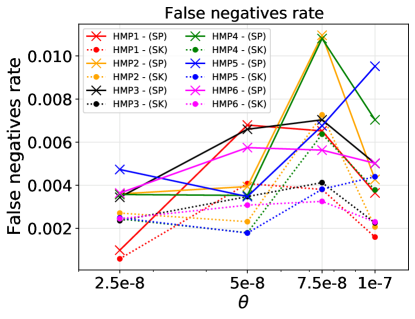
(a)

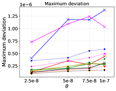
(b)

Figure S2: As function of $\theta$ and for every dataset: (a) False negatives rates, i.e. the fraction of $k$-mers of $FK(\mathcal{D},k,\theta)$ not reported by the approximation sets, obtained using $\mathsf{SPRISS}$ ($\mathsf{SP}$) and SAKEIMA ($\mathsf{SK}$); (b) Maximum deviations between exact and unbiased observed frequencies provided by the approximations sets of $\mathsf{SPRISS}$ ($\mathsf{SP}$) and SAKEIMA ($\mathsf{SK}$).

We use $\mathsf{SPRISS}$ to extract approximations of frequent $k$-mers on 6 datasets from HMP for values of the minimum frequency threshold $\theta\in\{2.5\cdot 10^{-8},5\cdot 10^{-8},7.5\cdot 10^{-8},10^{-7}\}$. The output of $\mathsf{SPRISS}$ satisfied the guarantees from Proposition 6 for all 5 runs of every combination of dataset and $\theta$. In all cases the estimated frequencies provided by $\mathsf{SPRISS}$ are close to the exact ones (see Figure 1a for an example). In fact, the average (across all reported $k$-mers) absolute deviation of the estimated frequency w.r.t. the true frequency is always small, i.e. one order of magnitude smaller than $\theta$ (Figure  1b), and the maximum deviations is very small as well (Figure S2b). In addition, $\mathsf{SPRISS}$ results in a very low false negative rate (i.e., fraction of $k$-mers of $FK(\mathcal{D},k,\theta)$ not reported by $\mathsf{SPRISS}$), which is always been below $0.012$ in our experiments.

In terms of running time, $\mathsf{SPRISS}$ required at most $64\%$ of the time required by the exact approach KMC (Figure 1c). This is due to $\mathsf{SPRISS}$ requiring to analyze at most $34\%$ of the entire dataset (Figure 1d). Note that the use of collections of bags of reads is crucial to achieve useful sample size, i.e. lower than the whole dataset: the sample size from Hoeffding’s inequality and union bound (Proposition 1), and the one from pseudodimension without collections of bags (Proposition 4) are $\approx 10^{16}$ and $\approx 10^{15}$, respectively, which are useless for datasets of $\approx 10^{8}$ reads. These results show that $\mathsf{SPRISS}$ obtains very accurate approximations of frequent $k$-mers in a fraction of the time required by exact counting approaches.

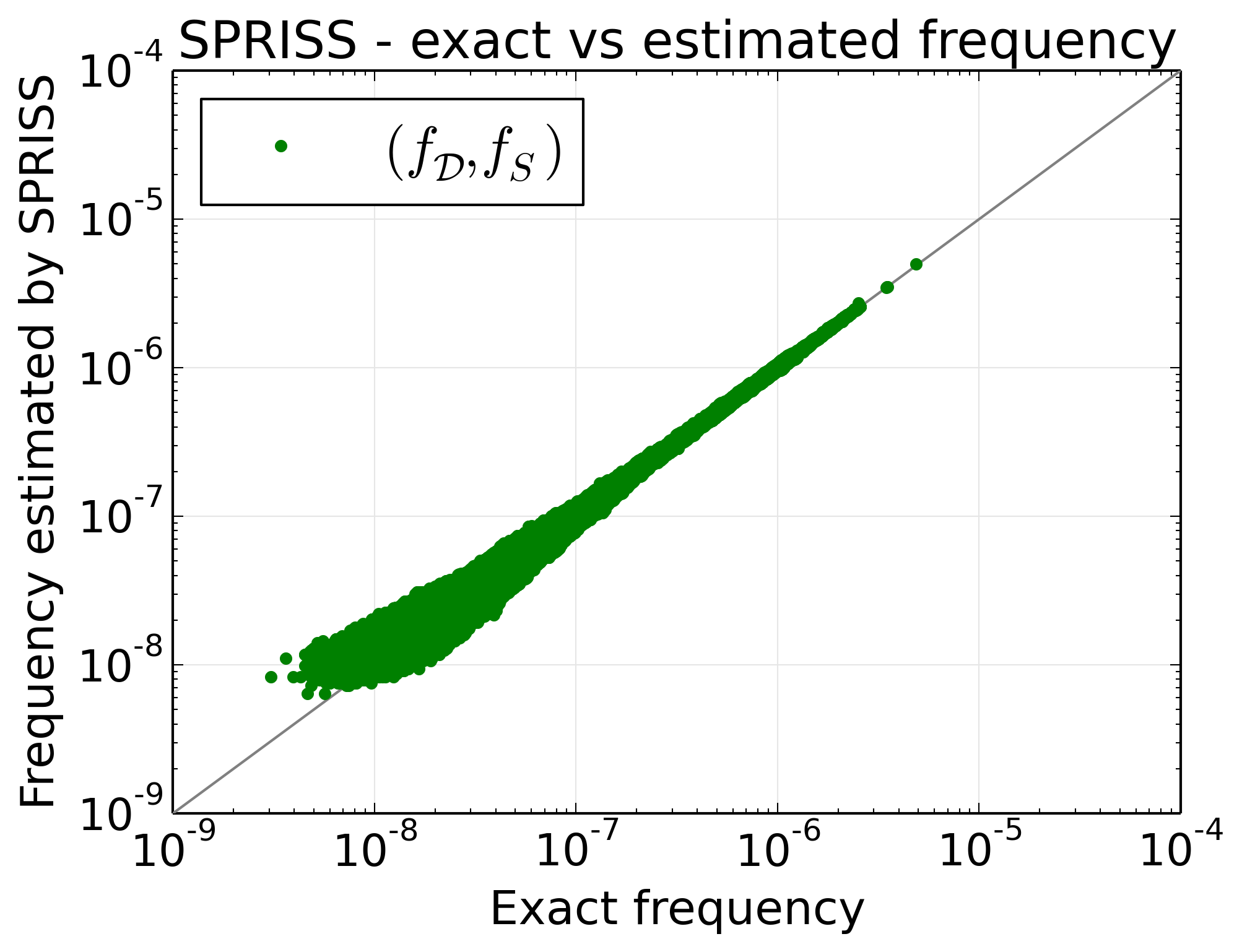
(a)

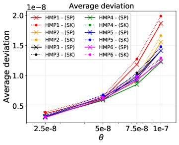
(b)

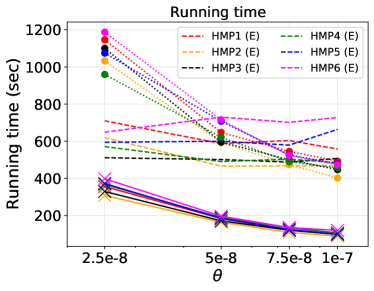
(c)

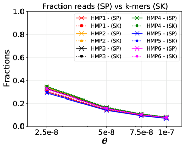
(d)

Figure 1: (a) $k$-mers exact frequency and frequency estimated by $\mathsf{SPRISS}$ for dataset SRS024075 and $\theta=2.5\cdot 10^{-8}$. (b) Average deviations between exact frequencies and frequencies estimated by $\mathsf{SPRISS}$ ($\mathsf{SP}$) and SAKEIMA ($\mathsf{SK}$), for various datasets and values of $\theta$. (c) Running time of $\mathsf{SPRISS}$ ($\mathsf{SP}$), SAKEIMA ($\mathsf{SK}$), and the exact computation ($\mathsf{E}$) - see also legend of panel 1b). (d) Fraction of the dataset analyzed by $\mathsf{SPRISS}$ ($\mathsf{SP}$) and by SAKEIMA ($\mathsf{SK}$).

We then compared $\mathsf{SPRISS}$ with SAKEIMA. In terms of quality of approximation, $\mathsf{SPRISS}$ reports approximations with an average deviation lower than SAKEIMA’s approximations, while SAKEIMA’s approximations have a lower maximum deviation. However, the ratio between the maximum deviation of $\mathsf{SPRISS}$ and the one of SAKEIMA are always below 2. Overall, the quality of the approximation provided by $\mathsf{SPRISS}$ and SAKEIMA are, thus, comparable. In terms of running time, $\mathsf{SPRISS}$ significantly improves over SAKEIMA (Figure 1c), and processes slightly smaller portions of the dataset compared to SAKEIMA (Figure 1d). Summarizing, $\mathsf{SPRISS}$ is able to report most of the frequent $k$-mers and estimate their frequencies with small errors, by analyzing small samples of the datasets and with significant improvements on running times compared to exact approaches and to state-of-the-art sampling algorithms.

6.3 Comparing Metagenomic Datasets

We evaluated $\mathsf{SPRISS}$ to compare metagenomic datasets by computing an approximation to the Bray-Curtis (BC) distance between pairs of datasets of reads, and using such approximations to cluster datasets.

Let $\mathcal{D}_{1}$ and $\mathcal{D}_{2}$ be two datasets of reads. Let $\mathcal{F}_{1}=FK(\mathcal{D}_{1},k,\theta)$ and $\mathcal{F}_{2}=FK(\mathcal{D}_{2},k,\theta)$ be the set of frequent $k$-mers respectively of $\mathcal{D}_{1}$ and $\mathcal{D}_{2}$, where $\theta$ is a minimum frequency threshold. The BC distance between $\mathcal{D}_{1}$ and $\mathcal{D}_{2}$ considering only frequent $k$-mers is defined as $BC(\mathcal{D}_{1},\mathcal{D}_{2},\mathcal{F}_{1},\mathcal{F}_{2})=1-2I/U$, where $I=\sum_{K\in\mathcal{F}_{1}\cap\mathcal{F}_{2}}\min\{o_{\mathcal{D}_{1}}(K),o_{\mathcal{D}_{2}}(K)\}$ and $U=\sum_{K\in\mathcal{F}_{1}}o_{\mathcal{D}_{1}}(K)+\sum_{K\in\mathcal{F}_{2}}o_{\mathcal{D}_{2}}(K).$ Conversely, the BC similarity is defined as $1-BC(\mathcal{D}_{1},\mathcal{D}_{2},\mathcal{F}_{1},\mathcal{F}_{2})$.

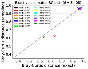
(a)

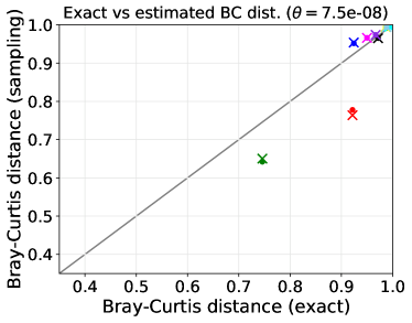
(b)

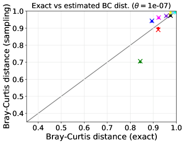
(c)

Figure S3: Comparison of the approximations of the Bray-Curtis distances using approximations of frequent $k$-mers sets provided by $\mathsf{SPRISS}$ ($\times$) and by SAKEIMA ($\bullet$) with the exact distances, for: (a) $\theta=5\cdot 10^{-8}$; (b) $\theta=7.5\cdot 10^{-8}$; (c) $\theta=1\cdot 10^{-7}$.

We considered 6 datasets from HMP, and estimated the BC distances among them by using $\mathsf{SPRISS}$ to approximate the sets of frequent $k$-mers $\mathcal{F}_{1}=FK(\mathcal{D}_{1},k,\theta)$ and $\mathcal{F}_{2}=FK(\mathcal{D}_{2},k,\theta)$ for the values of $\theta$ as in Section 6.2. We compared such estimated distances with the exact BC distances and with the estimates obtained using SAKEIMA. Both $\mathsf{SPRISS}$ and SAKEIMA provide accurate estimates of the BC distances (Figure 2a and Figure S3), which can be used to assess the relative similarity of pairs of datasets. However, to obtain such approximations $\mathsf{SPRISS}$ requires at most $25\%$ of the time required by SAKEIMA and usually $30\%$ of the time required by the exact computation with KMC(Figure 2b). Therefore $\mathsf{SPRISS}$ provides accurate estimates of metagenomic distances in a fraction of time required by other approaches.

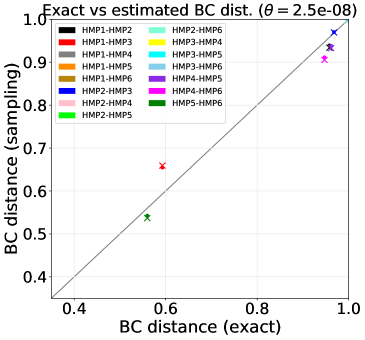
(a)

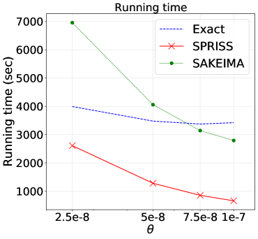
(b)

(c)

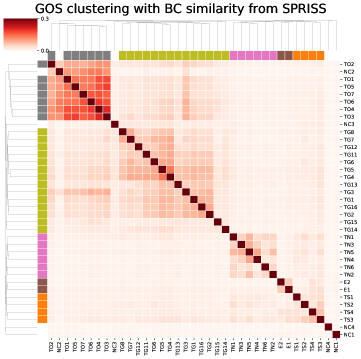
(d)

Figure 2: (a) Comparison of the approximations of the Bray-Curtis (BC) distances using approximations of frequent $k$-mers provided by $\mathsf{SPRISS}$ ($\times$) and by SAKEIMA ($\bullet$), and the exact distances, for $\theta=2.5\cdot 10^{-8}$. (b) Running time to approximate BC distances for all pairs of datasets with $\mathsf{SPRISS}$, with SAKEIMA, and the exact approach. (c) Average linkage hierarchical clustering of GOS datasets using Jaccard similarity. (d) Same as (c), using estimated BC similarity from $\mathsf{SPRISS}$ with $50\%$ of the data. (See also larger Figures S4-S6 in Supplemental Material for better readability of datasets’ labels and computed clusters.)

As an example of the impact in accurately estimating distances among metagenomic datasets, we used the sampling approach of $\mathsf{SPRISS}$ to approximate all pairwise BC distances among $37$ small datasets from the Sorcerer II Global Ocean Sampling Expedition (GOS) [48], and used such distances to cluster the datasets using average linkage hierarchical clustering. The $k$-mer based clustering of metagenomic datasets is often performed by using presence-based distances, such as the Jaccard distance [36], which estimates similarities between two datasets by computing the fraction of $k$-mers in common between the two datasets. Abundance-based distances, such as the BC distance [4, 11, 12], provide more detailed measures based also on the $k$-mers abundance, but are often not used due to the heavy computational requirements to extract all $k$-mers counts. However, the sampling approach of $\mathsf{SPRISS}$ can significantly speed-up the computation of all BC distances, and, thus, the entire clustering analysis. In fact, for this experiment, the use of $\mathsf{SPRISS}$ reduces the time required to analyze the datasets (i.e., obtain $k$-mers frequencies, compute all pairwise distances, and obtain the clustering) by $62\%$.

We then compared the clustering obtained using the Jaccard distance (Figure 2c) and the clustering obtained using the estimates of the BC distances (Figure 2d) obtained using only $50\%$ of reads in the GOS datasets, which are assigned to groups and macro-groups according to the origin of the sample [48]. Even if the BC distance is computed using only a sample of the datasets, while the Jaccard distance is computed using the entirety of all datasets, the use of approximate BC distances leads to a better clustering in terms of correspondence of clusters to groups, and to the correct cluster separation for macro-groups. In addition, the similarities among datasets in the same group and the dissimilarities among datasets in different groups are more accentuated using the approximated BC distance. In fact, the ratio between the average BC similarity among datasets in the same group and the analogous average Jaccard is in the interval $[1.25,1.75]$ for all groups. In addition, the ratio between i) the difference of the average BC similarity within the tropical macro-group and the average BC similarity between the tropical and temperate groups, and ii) the analogous difference using the Jaccard similarity is $\approx 1.53$. These results tell us the approximate BC-distances, computed using only half of the reads in each dataset, increase by $\approx 50\%$ the similarity signal inside all groups defined by the original study [48], and the dissimilarities between the two macro-groups (tropical and temperate).

To conclude, the estimates of the BC similarities obtained using the sampling scheme of $\mathsf{SPRISS}$ allows to better cluster metagenomic datasets than using the Jaccard similarity, while requiring less than $40\%$ of the time needed by the exact computation of BC similarities, even for fairly small metagenomic datasets.

6.4 Approximation of Discriminative $k$-mers

In this section we assess $\mathsf{SPRISS}$ for approximating discriminative $k$-mers in metagenomic datasets. In particular, we consider the following definition of discriminative $k$-mers [23]. Given two datasets $\mathcal{D}_{1},\mathcal{D}_{2}$, and a minimum frequency threshold $\theta$, we define the set $DK(\mathcal{D}_{1},\mathcal{D}_{2},k,\theta,\rho)$ of $\mathcal{D}_{1}$-discriminative $k$-mers as the collection of $k$-mers $K$ for which the following conditions both hold: 1. $K\in FK(\mathcal{D}_{1},k,\theta)$; 2. $f_{\mathcal{D}_{1}}(K)\geq\rho f_{\mathcal{D}_{2}}(K)$, with $\rho=2$. Note that the computation of $DK(\mathcal{D}_{1},\mathcal{D}_{2},k,\theta,\rho)$ requires to extract $FK(\mathcal{D}_{1},k,\theta)$ and $FK(\mathcal{D}_{2},k,\theta/\rho)$. $\mathsf{SPRISS}$ can be used to approximate the set $DK(\mathcal{D}_{1},\mathcal{D}_{2},k,\theta,\rho)$, by computing approximations $\overline{FK}(\mathcal{D}_{i},k,\theta)$ of the sets $FK(\mathcal{D}_{i},k,\theta)$, $i=1,2$, of frequent $k$-mers in $\mathcal{D}_{1},\mathcal{D}_{2}$, and then reporting a $k$-mer $K$ as $\mathcal{D}_{1}$-discriminative if the following conditions both hold: 1. $K\in\overline{FK}(\mathcal{D}_{1},k,\theta)$; 2. $K\notin\overline{FK}(\mathcal{D}_{2},k,\theta)$, or $f_{S^{1}_{\ell}}(K)\geq\rho f_{S^{2}_{\ell}}(K)$ when $K\in\overline{FK}(\mathcal{D}_{2},k,\theta)$.

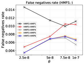
(c)

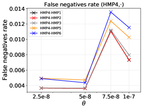
(d)

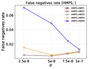
(e)

(f)

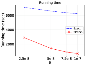
(g)

Figure S7: As function of $\theta$, false negatives rate, i.e. the fraction of $k$-mers of $DK(\mathcal{D}_{1},\mathcal{D}_{2},k,\theta,\rho)$ not included in its approximation $\overline{DK}(\mathcal{D}_{1},\mathcal{D}_{2},k,\theta,\rho)$, which is obtained using $\mathsf{SPRISS}$, for all pairs of datasets $\mathcal{D}_{1}$ and $\mathcal{D}_{2}$. Figure S7g shows the running times to compute $\overline{DK}(\mathcal{D}_{1},\mathcal{D}_{2},k,\theta,\rho)$ using $\mathsf{SPRISS}$ against the one required to compute the exact set $DK(\mathcal{D}_{1},\mathcal{D}_{2},k,\theta,\rho)$, cumulative for all pairs of datasets $\mathcal{D}_{1}$ and $\mathcal{D}_{2}$.

To evaluate such approach, we considered two datasets from [23], and $\theta=2\cdot 10^{-7}$ and $\rho=2$, which are the parameters used in [23]. We used the sampling approach of $\mathsf{SPRISS}$ with $\ell=\lfloor 0.02/(\theta\ell_{\mathcal{D},k})\rfloor$ and $\ell=\lfloor 0.04/(\theta\ell_{\mathcal{D},k})\rfloor$, resulting in analyzing of $5\%$ and $10\%$ of all reads, to approximate the sets of discriminative $\mathcal{D}_{1}$-discriminative and of $\mathcal{D}_{2}$-discriminative $k$-mers. When $5\%$ of the reads are used, the false negative rate is $<0.028$, while when $10\%$ of the reads are used, the false negative rate is $<0.018$. The running times are $\approx 1130$ sec. and $\approx 1970$ sec., respectively, while the exact computation of the discriminative $k$-mers with KMC requires $\approx 10^{4}$ sec. (we used 32 workers for both $\mathsf{SPRISS}$ and KMC). Similar results are obtained when analyzing pairs of HMP datasets, for various values of $\theta$ (Figure S7). These results show that $\mathsf{SPRISS}$ can identify discriminative $k$-mers with small false negative rates while providing a remarkable improvement in running time compared to the exact approach.

7 Conclusions

We presented $\mathsf{SPRISS}$, an efficient algorithm to compute rigorous approximations of frequent $k$-mers and their frequencies by sampling reads. $\mathsf{SPRISS}$ builds on pseudodimension, an advanced concept from statistical learning theory. Our extensive experimental evaluation shows that $\mathsf{SPRISS}$ provides high-quality approximations and can be employed to speed-up exploratory analyses in various applications, such as the analysis of metagenomic datasets and the identification of discriminative $k$-mers. Overall, the sampling approach used by $\mathsf{SPRISS}$ provides an efficient way to obtain a representative subset of the data that can be used to perform complex analyses more efficiently than examining the whole data, while obtaining representative results.

Supplemental Material

Appendix A Analysis of Simple Reads Sampling Algorithm

In this section we prove Proposition 1, which here corresponds to Proposition 10. To this aim, we need to introduce and prove some preliminary results.

Proposition 7.

The expectation $\mathbb{E}[t_{S,k}]$ of the size of the multiset of $k$-mers that appear in $S$ is $m\ell_{\mathcal{D},k}$.

Proof.

Let $X(r_{i})=n_{i}-k+1$ be the number of starting positions for $k$-mers in read $r_{i}$ sampled uniformly at random form $\mathcal{D}$, $i\in\{1,\dots,n\}$. $\mathbb{E}[X(r_{i})]=\sum_{r_{i}\in\mathcal{D}}\frac{1}{n}(n_{i}-k+1)=\ell_{\mathcal{D},k}$. Combining this with the linearity of the expectation, we have:

$$\mathbb{E}[t_{S,k}]=\mathbb{E}\left[\sum_{r_{i}\in S}(n_{i}-k+1)\right]=\sum_{r_{i}\in S}\mathbb{E}[n_{i}-k+1]=m\mathbb{E}[X(r_{i})]=m\ell_{\mathcal{D},k}.$$

∎

Given a $k$-mer $K$, its support $o_{S}(K)$ in $S$ is defined as $o_{S}(K)=\sum_{r_{i}\in S}\sum_{j=0}^{n_{i}-k}\phi_{r_{i},K}(j)$. We define the frequency of $K$ in $S$ as $f_{S}(K)=o_{S}(K)/(m\ell_{\mathcal{D},k})$, that is the ratio between the support of $K$ and the expectation $\mathbb{E}[t_{S,k}]=m\ell_{\mathcal{D},k}$ of the size of the multiset of $k$-mers that appear in $S$. This definition of $f_{S}(K)$ gives us an unbiased estimator for $f_{\mathcal{D}}(K)$.

Proposition 8.

The frequency $f_{S}(K)=o_{S}(K)/(m\ell_{\mathcal{D},k})$ is an unbiased estimator for $f_{\mathcal{D}}(K)=o_{\mathcal{D}}(K)/t_{\mathcal{D},k}$.

Proof.

Let $X_{r_{i}}(K)=\sum_{j=0}^{n_{i}-k}\phi_{r_{i},K}(j)$ be the number of distinct positions where $k$-mer $K$ appears in read $r_{i}$ sampled uniformly at random form $\mathcal{D}$, $i\in\{1,\dots,n\}$. $E[X_{r_{i}}(K)]=\sum_{r_{i}\in\mathcal{D}}\left(\frac{1}{n}\sum_{j=0}^{n_{i}-k}\phi_{r_{i},K}(j)\right)=o_{\mathcal{D}}(K)/n.$ Combining this with the linearity of the expectation, we have:

$$\mathbb{E}[f_{S}(K)]=\frac{E[o_{S}(K)]}{m\ell_{\mathcal{D},k}}=\frac{\mathbb{E}[\sum_{r_{i}\in S}\sum_{j=0}^{n_{i}-k}\phi_{r_{i},K}(j)]}{m\ell_{\mathcal{D},k}}=\frac{\mathbb{E}[X_{r_{i}}(K)]}{\ell_{\mathcal{D},k}}=\frac{o_{\mathcal{D}}(K)}{n\ell_{\mathcal{D},k}}=\frac{o_{\mathcal{D}}(K)}{t_{\mathcal{D},k}}=f_{\mathcal{D}}(K).$$

∎

By using the sampling framework based on reads and the Hoeffding inequality [33], we prove the following bound on the probability that $f_{S}(K)$ is not within $\varepsilon/2$ from $f_{\mathcal{D}}(K)$, for an arbitrary $k$-mer $K$.

Proposition 9.

Consider a sample $S$ of $m$ reads from $\mathcal{D}$. Let $\ell_{\max,\mathcal{D},k}=\max_{r_{i}\in\mathcal{D}}(n_{i}-k+1)$. Let $K\in\Sigma^{k}$ be an arbitrary $k$-mer. For a fixed accuracy parameter $\varepsilon\in(0,1)$ we have:

$$\Pr\left(|f_{S}(K)-f_{\mathcal{D}}(K)|\geq\frac{\varepsilon}{2}\right)\leq 2\exp\left(-\frac{1}{2}m\varepsilon^{2}\left(\frac{\ell_{\mathcal{D},k}}{\ell_{\max,\mathcal{D},k}}\right)^{2}\right).$$ (2)

Proof.

The frequency $f_{S}(K)=o_{S}(K)/(m\ell_{\mathcal{D},k})$ of $K$ in $S$ can be rewritten as:

$$f_{S}(K)=\frac{\sum_{r_{i}\in S}\sum_{j=0}^{n_{i}-k}\phi_{r_{i},K}(j)}{m\ell_{\mathcal{D},k}}=\sum_{r_{i}\in S}\sum_{j=0}^{n_{i}-k}\frac{\phi_{r_{i},K}(j)}{m\ell_{\mathcal{D},k}}=\sum_{r_{i}\in S}\hat{\phi}_{K}(r_{i}),$$ (3)

where the random variable (r.v.) $\hat{\phi}_{K}(r_{i})=\sum_{j=0}^{n_{i}-k}\frac{\phi_{r_{i},K}(j)}{m\ell_{\mathcal{D},k}}$ is the number of times $K$ appears in read $r_{i}$ divided by $m\ell_{\mathcal{D},k}$. Thus, $f_{S}(K)$ can be rewritten as a sum of $m$ independent r.v. that take values in $[0,\frac{\ell_{\max,\mathcal{D},k}}{m\ell_{\mathcal{D},k}}]$. Combining this fact with Proposition 8, and by applying the Hoeffding inequality [33] we have:

$$\Pr(|f_{S}(K)-f_{\mathcal{D}}(K)|\geq\frac{\varepsilon}{2})\leq 2\exp\left(\frac{-2(\varepsilon/2)^{2}}{m\left(\frac{\ell_{\max,\mathcal{D},k}}{m\ell_{\mathcal{D},k}}\right)^{2}}\right)=2\exp\left(-\frac{1}{2}m\varepsilon^{2}\left(\frac{\ell_{\mathcal{D},k}}{\ell_{\max,\mathcal{D},k}}\right)^{2}\right).$$

∎

Since the maximum number of $k$-mers is $\sigma^{k}$, by combining the result above with the union bound we have the following result.

Proposition 10.

Consider a sample $S$ of $m$ reads from $\mathcal{D}$. For fixed frequency threshold $\theta\in(0,1]$, error parameter $\varepsilon\in(0,\theta)$, and confidence parameter $\delta\in(0,1)$, if

$$m\geq\frac{2}{\varepsilon^{2}}\left(\frac{\ell_{\max,\mathcal{D},k}}{\ell_{\mathcal{D},k}}\right)^{2}\left(\ln\left(2\sigma^{k}\right)+\ln\left(\frac{1}{\delta}\right)\right)$$ (4)

then, with probability $\geq 1-\delta$, $FK(S,k,\theta-\varepsilon/2)$ is an $\varepsilon$-approximation of $FK(\mathcal{D},k,\theta)$.

Proof.

Let $E_{K}$ be the event “$|f_{S}(K)-f_{\mathcal{D}}(K)|\leq\frac{\varepsilon}{2}$” for a $k$-mer $K$. By the choice of $m$ and Proposition 9 we have that the probability of the complementary event $\overline{E}_{K}$ of $E_{K}$ is

$$\Pr(\overline{E}_{K})=\Pr\left(|f_{S}(K)-f_{\mathcal{D}}(K)|\geq\frac{\varepsilon}{2}\right)=2\exp\left(-\frac{1}{2}m\varepsilon^{2}\left(\frac{\ell_{\mathcal{D},k}}{\ell_{\max,\mathcal{D},k}}\right)^{2}\right)\leq\frac{\delta}{\sigma^{k}}.$$

Now, by applying the union bound, the probability that for at least one $k$-mer $K$ of $\Sigma^{k}$ the event $\overline{E}_{K}$ holds is bounded by $\sum_{K\in\Sigma^{k}}\Pr(\overline{E}_{K})\leq\delta$. Thus, the probability that events $E_{K}$ simultaneously hold for all $k$-mers $K$ in $\Sigma^{k}$ is at least $1-\delta$.

Now we prove that, with probability at least $1-\delta$, $FK(S,k,\theta-\varepsilon/2)$ is an $\varepsilon$-approximation of $FK(\mathcal{D},k,\theta)$, when, with probability at least $1-\delta$, “$|f_{S}(K)-f_{\mathcal{D}}(K)|\leq\frac{\varepsilon}{2}$” for all $k$-mers $K$. Note that the third property of Definition 1 is already satisfied. Let $K$ be a $k$-mer of $FK(\mathcal{D},k,\theta)$, that is $f_{\mathcal{D}}(K)\geq\theta$. Given that $f_{S}(K)\geq f_{\mathcal{D}}(K)-\varepsilon/2$, we have $f_{S}(K)\geq\theta-\varepsilon/2$ and the first property of Definition 1 holds. Combining $f_{\mathcal{D}}(K)\geq f_{S}(K)-\varepsilon/2$ and $f_{S}(K)\geq\theta-\varepsilon/2$, we have $f_{\mathcal{D}}(K)\geq\theta-\varepsilon$ and the second property of Definition 1 holds. ∎

The previous theorem gives us the following simple procedure for approximating the set of frequent $k$-mers with guarantees on the quality of the solution: build a sample $S$ of $m\geq\frac{2}{\varepsilon^{2}}\left(\frac{\ell_{\max,\mathcal{D},k}}{\ell_{\mathcal{D},k}}\right)^{2}\left(\ln\left(2\sigma^{k}\right)+\ln\left(\frac{1}{\delta}\right)\right)$ reads from $\mathcal{D}$, and output the set $FK(S,k,\theta-\varepsilon/2)$ which is an $\varepsilon$-approximation of $FK(\mathcal{D},k,\theta)$ with probability at least $1-\delta$. Since the frequencies of $k$-mers we are estimating are small, then $\epsilon$ must be set to a small value. This typically results in a sample size $m$ larger than $|\mathcal{D}|$, making useless the sampling approach.

Appendix B Analysis of the First Improvement: A Pseudodimension-based Algorithm for $k$-mers Approximation by Sampling Reads

In this section we prove Proposition 3 and Proposition 4, which here corresponds to Proposition 12 and Proposition 13, respectively. In order to help the reader to avoid too many jumps to the main text, we reintroduce some important definitions and results.

Let $\mathcal{F}$ be a class of real-valued functions from a domain $X$ to $[a,b]\subset\mathbb{R}$. Consider, for each $f\in\mathcal{F}$, the subset of $X^{\prime}=X\times[a,b]$ defined as $R_{f}=\{(x,t):t\leq f(x)\}$, and call it range. Let $\mathcal{F}^{+}=\{R_{f},f\in\mathcal{F}\}$ be a range set on $X^{\prime}$, and its corresponding range space $Q^{\prime}$ be $Q^{\prime}=(X^{\prime},\mathcal{F}^{+})$. We say that a subset $D\subset X^{\prime}$ is shattered by $\mathcal{F}^{+}$ if the size of the projection set $proj_{\mathcal{F}^{+}}(D)=\{r\cap D:r\in\mathcal{F}^{+}\}$ is equal to $2^{|D|}$. The VC dimension $VC(Q^{\prime})$ of $Q^{\prime}$ is the maximum size of a subset of $X^{\prime}$ shattered by $\mathcal{F}^{+}$. The pseudodimension $PD(X,\mathcal{F})$ is then defined as the VC dimension of $Q^{\prime}$: $PD(X,\mathcal{F})=VC(Q^{\prime})$.

Let $\pi$ the uniform distribution on $X$, and let $S$ be a sample of $X$ of size $|S|=m$, with every element of $S$ sampled independently and uniformly at random from $X$. We define, $\forall f\in\mathcal{F}$, $f_{S}=\frac{1}{m}\sum_{x\in S}f(x)$ and $f_{X}=\mathbb{E}_{x\sim\pi}[f(x)]$. Note that $\mathbb{E}[f_{S}]=f_{X}$. The following result relates the accuracy and confidence parameters $\varepsilon$,$\delta$ and the pseudodimension with the probability that the expected values of the functions in $\mathcal{F}$ are well approximated by their averages computed from a finite random sample.

Proposition 11 ([56, 25]).

Let $X$ be a domain and $\mathcal{F}$ be a class of real-valued functions from $X$ to $[a,b]$. Let $PD(X,\mathcal{F})=VC(Q^{\prime})\leq v$. There exist an absolute positive constant $c$ such that, for fixed $\varepsilon,\delta\in(0,1)$, if $S$ is a random sample of $m$ samples drawn independently and uniformly at random from $X$ with

$$m\geq\frac{c\left(b-a\right)^{2}}{\varepsilon^{2}}\left(v+\ln\left(\frac{1}{\delta}\right)\right)$$ (5)

then, with probability $\geq 1-\delta$, it holds simultaneously $\forall f\in\mathcal{F}$ that $|f_{S}-f_{X}|\leq\varepsilon$.

The universal constant $c$ has been experimentally estimated to be at most $0.5$ [24].

Here we define the range space associated to $k$-mers and derive an upper bound to its pseudodimension. Finally, we derive a tighter sample size compared to the one proposed in Proposition 10.

The definition of the range space $Q^{\prime}=(X^{\prime},\mathcal{F}^{+})$ associated to $k$-mers requires to define the domain $X$ and the class of real-valued functions $\mathcal{F}$.

Definition 3.

Let $k$ be a positive integer and $\mathcal{D}$ be a bag of $n$ reads. Define the domain $X$ as the set of integers $\{1,\dots,n\}$, where every $i\in X$ corresponds to the $i$-th read of $\mathcal{D}$. Then define the family of real-valued functions $\mathcal{F}=\{f_{K},\forall K\in\Sigma^{k}\}$ where, for every $i\in X$ and for every $f_{K}\in\mathcal{F}$, the function $f_{K}(i)$ is the number of distinct positions in read $r_{i}$ where $k$-mer $K$ appears divided by the average size of the multiset of $k$-mers that appear in a read of $\mathcal{D}$: $f_{K}(i)=\sum_{j=0}^{n_{i}-k}\frac{\phi_{r_{i},K}(j)}{\ell_{\mathcal{D},k}}$. Therefore $f_{K}(i)\in[0,\frac{\ell_{\max,\mathcal{D},k}}{\ell_{\mathcal{D},k}}]$. For each $f_{K}\in\mathcal{F}$, the subset of $X^{\prime}=X\times[0,\frac{\ell_{\max,\mathcal{D},k}}{\ell_{\mathcal{D},k}}]$ defined as $R_{f_{K}}=\{(i,t):t\leq f_{K}(i)\}$ is the associated range. Let $\mathcal{F}^{+}=\{R_{f_{K}},f_{K}\in\mathcal{F}\}$ be the range set on $X^{\prime}$, and its corresponding range space $Q^{\prime}$ be $Q^{\prime}=(X^{\prime},\mathcal{F}^{+})$.

A trivial upper bound to $PD(X,\mathcal{F})$ is given by $PD(X,\mathcal{F})\leq\lfloor\log_{2}|\mathcal{F}|\rfloor=\lfloor\log_{2}\sigma^{k}\rfloor$. Before proving a tighter bound to $PD(X,\mathcal{F})$, we first state a technical Lemma (Lemma 3.8 from [45].

Lemma 1.

Let $B\subseteq X^{\prime}$ be a set that is shattered by $\mathcal{F}^{+}$. Then $B$ does not contain any element in the form $(i,0)$, for any $i\in X$.

Proposition 12.

Let $\mathcal{D}$ be a bag of $n$ reads, $k$ a positive integer, $X$ be the domain and $\mathcal{F}$ be the family of real-valued functions defined in Definition 3. Then the pseudodimension $PD(X,\mathcal{F})$ satisfies

$$PD(X,\mathcal{F})\leq\lfloor\log_{2}(\ell_{max,\mathcal{D},k})\rfloor+1.$$ (6)

Proof.

From the definition of pseudodimension we have $PD(X,\mathcal{F})=VC(Q^{\prime})$, therefore showing $VC(Q^{\prime})=v\leq\lfloor\text{log}_{2}(\ell_{max,\mathcal{D},k})\rfloor+1$ is sufficient for the proof. An immediate consequence of Lemma 1 is that for all elements $(i,t)$ of any set $B$ that is shattered by $\mathcal{F}^{+}$ it holds $t\geq 1/\ell_{\mathcal{D},k}$. Now we denote an integer $v$ and suppose that $VC(Q^{\prime})=v$. Thus, there must exist a set $B\subseteq X^{\prime}$ with $|B|=v$ which needs to be shattered by $\mathcal{F}^{+}$. This means that $2^{v}$ subsets of $B$ must be in projection of $\mathcal{F}^{+}$ on $B$. If this is true, then every element of $B$ needs to belong to exactly $2^{v-1}$ such sets. This means that for a given $(i,t)$ of $B$, all the projections of $2^{v-1}$ elements of $\mathcal{F}^{+}$ contain $(i,t)$. Since $t\geq 1/\ell_{\mathcal{D},k}$, there need to exist $2^{v-1}$ distinct $k$-mers appearing at least once in the read $r_{i}$. More formally, it needs to hold $n_{i}-k+1\geq 2^{v-1}$, that implies $v\leq\lfloor\text{log}_{2}(n_{i}-k+1)\rfloor+1$, $\forall(i,t)\in B$. Since $n_{i}-k+1\leq\ell_{max,\mathcal{D},k}$ for each $(i,t)\in B$, then $v\leq\lfloor\text{log}_{2}(\ell_{max,\mathcal{D},k})\rfloor+1$, and the thesis holds. ∎

Based on the previous result, we obtain the following.

Proposition 13.

Consider a sample $S$ of $m$ reads from $\mathcal{D}$. For fixed frequency threshold $\theta\in(0,1]$, error parameter $\varepsilon\in(0,\theta)$, and confidence parameter $\delta\in(0,1)$, if

$$m\geq\frac{2}{\varepsilon^{2}}\left(\frac{\ell_{\max,\mathcal{D},k}}{\ell_{\mathcal{D},k}}\right)^{2}\left(\lfloor\log_{2}\min(2\ell_{\max,\mathcal{D},k},\sigma^{k})\rfloor+\ln\left(\frac{1}{\delta}\right)\right)$$ (7)

then, with probability $\geq 1-\delta$, $FK(S,k,\theta-\varepsilon/2)$ is an $\varepsilon$-approximation of $FK(\mathcal{D},k,\theta)$.

Proof.

Let consider the domain $X$ and the class of real-valued functions $\mathcal{F}$ defined in Definition 3. For a given function $f\in\mathcal{F}$ (so for a given $k$-mer $K$), we have for $f_{X}=\mathbb{E}_{x\sim\pi}[f(x)]$ that

$$f_{X}=\mathbb{E}_{r_{i}\sim\mathcal{D}}[f_{K}(i)]=\mathbb{E}_{r_{i}\sim\mathcal{D}}\left[\sum_{j=0}^{n_{i}-k}\frac{\phi_{r_{i},K}(j)}{\ell_{\mathcal{D},k}}\right]=\frac{1}{\ell_{\mathcal{D},k}}\sum_{r_{i}\in\mathcal{D}}\frac{1}{n}\sum_{j=0}^{n_{i}-k}\phi_{r_{i},K}(j)=\frac{o_{D}(K)}{n\ell_{\mathcal{D},k}}=f_{\mathcal{D}}(K),$$

and for $f_{S}=\frac{1}{m}\sum_{x\in S}f(x)$ that

$$f_{S}=\frac{1}{m}\sum_{r_{i}\in S}f_{K}(i)=\frac{1}{m}\sum_{r_{i}\in S}\sum_{j=0}^{n_{i}-k}\frac{\phi_{r_{i},K}(j)}{\ell_{\mathcal{D},k}}=\frac{o_{S}(K)}{m\ell_{\mathcal{D},k}}=f_{S}(K).$$

Combining the trivial bound $PD(X,\mathcal{F})\leq\lfloor\log_{2}\sigma^{k}\rfloor$ with Propositions 2 and 3 we have that, with probability at least $1-\delta$, $|f_{S}(K)-f_{\mathcal{D}}(K)|\leq\varepsilon/2$ simultaneously holds for every $k$-mer $K$.

Now, as for Proposition 10, we prove that, with probability at least $1-\delta$, $FK(S,k,\theta-\varepsilon/2)$ is an $\varepsilon$-approximation of $FK(\mathcal{D},k,\theta)$, when, with probability at least $1-\delta$, “$|f_{S}(K)-f_{\mathcal{D}}(K)|\leq\frac{\varepsilon}{2}$” for all $k$-mers $K$. Note that the third property of Definition 1 is already satisfied. Let $K$ be a $k$-mer of $FK(\mathcal{D},k,\theta)$, that is $f_{\mathcal{D}}(K)\geq\theta$. Given that $f_{S}(K)\geq f_{\mathcal{D}}(K)-\varepsilon/2$, we have $f_{S}(K)\geq\theta-\varepsilon/2$ and the first property of Definition 1 holds. Combining $f_{\mathcal{D}}(K)\geq f_{S}(K)-\varepsilon/2$ and $f_{S}(K)\geq\theta-\varepsilon/2$, we have $f_{\mathcal{D}}(K)\geq\theta-\varepsilon$ and the second property of Definition 1 holds. ∎

This bound significantly improves on the result of Proposition 10, since the factor $\ln(2\sigma^{k})$ has been reduced to $\lfloor\log_{2}\min(2\ell_{\max,\mathcal{D},k},\sigma^{k})\rfloor$. Finally, by taking a sample $S$ of size $m$ according to Proposition 13 and by extracting the set $FK(S,k,\theta-\varepsilon/2)$ we get an $\varepsilon$-approximation of $FK(\mathcal{D},k,\theta)$ with probability at least $1-\delta$. However, also this approach typically results in a sample size $m$ larger than $|\mathcal{D}|$.

Appendix C Analysis of the Main Technical Result (Proposition 6)

This section is dedicated to prove our main technical result on which $\mathsf{SPRISS}$ is built, i.e. Proposition 6 (here it corresponds to Proposition 17). We also prove Proposition 5 of the main text (here Proposition 14) and some additional but necessary results. As for the previous section, we reintroduce some important definitions and results.

We define $I_{\ell}=\{i_{1},i_{2},\dots,i_{\ell}\}$ as a bag of $\ell$ indexes of reads of $\mathcal{D}$ chosen uniformly at random, with replacement, from the set $\{1,\dots,n\}$. Then we define an $\ell$-reads sample $S_{\ell}$ as a bag of $m$ bags of $\ell$ reads $S_{\ell}=\{I_{\ell,1},\dots,I_{\ell,m}\}$. The definition of a new range space $Q^{\prime}=(X^{\prime},\mathcal{F}^{+})$ associated to $k$-mers requires to define a new domain $X$ and a new class of real-valued functions $\mathcal{F}$.

Definition 4.

Let $k$ be a positive integer and $\mathcal{D}$ be a bag of $n$ reads. Define the domain $X$ as the set of bags of $\ell$ indexes of reads of $\mathcal{D}$. Then define the family of real-valued functions $\mathcal{F}=\{f_{K,\ell},\forall K\in\Sigma^{k}\}$ where, for every $I_{\ell}\in X$ and for every $f_{K,\ell}\in\mathcal{F}$, we have $f_{K,\ell}(I_{\ell})=\min(1,o_{I_{\ell}}(K))/(\ell\ell_{\mathcal{D},k})$, where $o_{I_{\ell}}(K)=\sum_{i\in I_{\ell}}\sum_{j=0}^{n_{i}-k}\phi_{r_{i},K}(j)$ counts the number of occurrences of $K$ in all the $\ell$ reads of $I_{\ell}$. Therefore $f_{K,\ell}(I_{\ell})\in\{0,\frac{1}{\ell\ell_{\mathcal{D},k}}\}$ $\forall f_{K,\ell}$ and $\forall I_{\ell}$. For each $f_{K,\ell}\in\mathcal{F}$, the subset of $X^{\prime}=X\times\{0,\frac{1}{\ell\ell_{\mathcal{D},k}}\}$ defined as $R_{f_{K,\ell}}=\{(I_{\ell},t):t\leq f_{K,\ell}(I_{\ell})\}$ is the associated range. Let $\mathcal{F}^{+}=\{R_{f_{K,\ell}},f_{K,\ell}\in\mathcal{F}\}$ be the range set on $X^{\prime}$, and its corresponding range space $Q^{\prime}$ be $Q^{\prime}=(X^{\prime},\mathcal{F}^{+})$.

Note that, for a given bag $I_{\ell}$, the functions $f_{K,\ell}$ are then biased if $K$ appears more than $1$ times in all the $\ell$ reads of $I_{\ell}$. We now prove an upper bound to the pseudodimension $PD(X,\mathcal{F})$.

Proposition 14.

Let $\mathcal{D}$ be a bag of $n$ reads, $k$ a positive integer, $X$ be the domain and $\mathcal{F}$ be the family of real-valued functions defined in Definition 4. Then the pseudodimension $PD(X,\mathcal{F})$ satisfies

$$PD(X,\mathcal{F})\leq\lfloor\text{log}_{2}(\ell\ell_{max,\mathcal{D},k})\rfloor+1.$$ (8)

Proof.

From the definition of pseudodimension we have $PD(X,\mathcal{F})=VC(Q^{\prime})$, therefore showing $VC(Q^{\prime})=v\leq\lfloor\text{log}_{2}(\ell\ell_{max,\mathcal{D},k})\rfloor+1$ is sufficient for the proof. Since Lemma 1 is also valid for the new definition of the range space $Q^{\prime}=(X^{\prime},\mathcal{F}^{+})$, an immediate consequence is that for all elements $(i,t)$ of any set $B$ that is shattered by $\mathcal{F}^{+}$ it holds $t\geq 1/(\ell\ell_{\mathcal{D},k})$. Now we denote an integer $v$ and suppose that $VC(Q^{\prime})=v$. Thus, there must exist a set $B\subseteq X^{\prime}$ with $|B|=v$ which needs to be shattered by $\mathcal{F}^{+}$. This means that $2^{v}$ subsets of $B$ must be in projection of $\mathcal{F}^{+}$ on $B$. If this is true, then every element of $B$ needs to belong to exactly $2^{v-1}$ such sets. This means that for a given $(I_{\ell},t)$ of $B$, all the projections of $2^{v-1}$ elements of $\mathcal{F}^{+}$ contain $(I_{\ell},t)$. Since $t\geq 1/(\ell\ell_{\mathcal{D},k})$, there need to exist $2^{v-1}$ distinct $k$-mers appearing at least once in the bag of $\ell$ reads associated with $I_{\ell}$. More formally, it needs to hold $\sum_{i\in I_{\ell}}(n_{i}-k+1)\geq 2^{v-1}$, that implies $v\leq\lfloor\text{log}_{2}\sum_{i\in I_{\ell}}(n_{i}-k+1)\rfloor+1$, $\forall(I_{\ell},t)\in B$. Since $n_{i}-k+1\leq\ell_{max,\mathcal{D},k}$ for each $(I_{\ell},t)\in B$ and $i\in I_{\ell}$, then $v\leq\lfloor\text{log}_{2}(\ell\ell_{max,\mathcal{D},k})\rfloor+1$, and the thesis holds. ∎

Before showing an improved bound on the sample size, we need to define the frequency $\hat{f}_{S_{\ell}}(K)$ of a $k$-mer $K$ computed from the sample $S_{\ell}$:

$$\hat{f}_{S_{\ell}}(K)=\frac{1}{m}\sum_{I_{\ell,i}\in S_{\ell}}f_{K,\ell}(I_{\ell,i}),$$ (9)

which is the bias version of

$$f_{S_{\ell}}(K)=\frac{1}{m}\sum_{I_{\ell,i}\in S_{\ell}}o_{I_{\ell}}(K)/(\ell\ell_{\mathcal{D},k}).$$ (10)

Note that $\mathbb{E}[f_{S_{\ell}}(K)]=f_{\mathcal{D}}(K)$. In order to find a relation between $\mathbb{E}[\hat{f}_{S_{\ell}}(K)]$ and $f_{\mathcal{D}}(K)$, we need the following proposition.

Proposition 15.

Let $\tilde{f}_{\mathcal{D}}(K)=\sum_{r_{i}\in\mathcal{D}}\mathbbm{1}(K\in r_{i})/n$ and $f_{\mathcal{D}}(K)=o_{\mathcal{D}}(K)/t_{\mathcal{D},k}$. It holds that:

$$\frac{\ell_{\mathcal{D},k}}{\ell_{\max,\mathcal{D},k}}f_{\mathcal{D}}(K)\leq\tilde{f}_{\mathcal{D}}(K)\leq\ell_{\mathcal{D},k}f_{\mathcal{D}}(K).$$ (11)

Proof.

Let us rewrite $\tilde{f}_{\mathcal{D}}(K)$:

$$\tilde{f}_{\mathcal{D}}(K)=\sum_{r_{i}\in\mathcal{D}}\mathbbm{1}(K\in r_{i})/n=\frac{\mathbbm{1}(K\in r_{1})}{\ell_{\mathcal{D},k}}\frac{\ell_{\mathcal{D},k}}{n}+\dots+\frac{\mathbbm{1}(K\in r_{n})}{\ell_{\mathcal{D},k}}\frac{\ell_{\mathcal{D},k}}{n}.$$ (12)

Since $\mathbbm{1}(K\in r_{i})\leq o_{r_{i}}(K)$ for every $i\in\{1,\dots,n\}$, we have

$$\tilde{f}_{\mathcal{D}}(K)\leq\frac{o_{r_{1}}(K)}{\ell_{\mathcal{D},k}}\frac{\ell_{\mathcal{D},k}}{n}+\dots+\frac{o_{r_{n}}(K)}{\ell_{\mathcal{D},k}}\frac{\ell_{\mathcal{D},k}}{n}=\ell_{\mathcal{D},k}f_{\mathcal{D}}(K).$$ (13)

Since $\mathbbm{1}(K\in r_{i})\geq o_{r_{i}}(K)/\ell_{\max,\mathcal{D},k}$ for every $i\in\{1,\dots,n\}$, we have

$$\tilde{f}_{\mathcal{D}}(K)\geq\frac{o_{r_{1}}(K)}{n\ell_{\mathcal{D},k}}\frac{\ell_{\mathcal{D},k}}{\ell_{\max,\mathcal{D},k}}+\dots+\frac{o_{r_{n}}(K)}{n\ell_{\mathcal{D},k}}\frac{\ell_{\mathcal{D},k}}{\ell_{\max,\mathcal{D},k}}=\frac{\ell_{\mathcal{D},k}}{\ell_{\max,\mathcal{D},k}}f_{\mathcal{D}}(K).$$ (14)

∎

Now we show a relation between $\mathbb{E}[\hat{f}_{S_{\ell}}(K)]$ and $f_{\mathcal{D}}(K)$.

Proposition 16.

Let $\tilde{f}_{\mathcal{D}}(K)=\sum_{r_{i}\in\mathcal{D}}\mathbbm{1}(K\in r_{i})/n$ and $f_{\mathcal{D}}(K)=o_{\mathcal{D}}(K)/t_{\mathcal{D},k}$. Let $S_{\ell}$ be a bag of $m$ bags of $\ell$ reads drawn from $\mathcal{D}$. Then:

$$\mathbb{E}[\hat{f}_{S_{\ell}}(K)]\geq\frac{1}{\ell\ell_{\mathcal{D},k}}(1-(1-\frac{\ell_{\mathcal{D},k}}{\ell_{\max,\mathcal{D},k}}f_{\mathcal{D}}(K))^{\ell}).$$ (15)

Proof.

Let us rewrite $\mathbb{E}[\hat{f}_{S_{\ell}}(K)]$:

$$\mathbb{E}[\hat{f}_{S_{\ell}}(K)]=\frac{1}{\ell\ell_{\mathcal{D},k}}\mathbb{E}[\min(1,o_{I_{\ell}}(K))]=\frac{1}{\ell\ell_{\mathcal{D},k}}\Pr(o_{I_{\ell}}(K)>0).$$ (16)

Then, we have

$$\mathbb{E}[\hat{f}_{S_{\ell}}(K)]=\frac{1}{\ell\ell_{\mathcal{D},k}}Pr(o_{I_{\ell}}(K)>0)=\frac{1}{\ell\ell_{\mathcal{D},k}}(1-Pr(o_{I_{\ell}}(K)=0))=$$ (17)

$$=\frac{1}{\ell\ell_{\mathcal{D},k}}(1-\prod_{i\in I_{\ell}}\Pr(o_{r_{i}}(K)=0))=\frac{1}{\ell\ell_{\mathcal{D},k}}(1-(1-\tilde{f}_{\mathcal{D}}(K))^{\ell}),$$ (18)

and since $\tilde{f}_{\mathcal{D}}(K)\geq\frac{\ell_{\mathcal{D},k}}{\ell_{\max,\mathcal{D},k}}f_{\mathcal{D}}(K)$ by Proposition 15, the thesis holds. ∎

Let $\theta$ be a minimum frequency threshold. Using the previous proposition, if

$$f_{\mathcal{D}}(K)\geq\frac{\ell_{\max,\mathcal{D},k}}{\ell_{\mathcal{D},k}}(1-(1-\ell\ell_{\mathcal{D},k}\theta)^{1/\ell})$$ (19)

with $\ell\leq 1/(\ell_{\mathcal{D},k}\theta)$, then $\mathbb{E}[\hat{f}_{S_{\ell}}(K)]\geq\theta$.

Proposition 17.

Let $k$ and $\ell$ be two positive integers. Consider a sample $S_{\ell}$ of $m$ bags of $\ell$ reads from $\mathcal{D}$. For fixed frequency threshold $\theta\in(0,1]$, error parameter $\varepsilon\in(0,\theta)$, and confidence parameter $\delta\in(0,1)$, if

$$m\geq\frac{2}{\varepsilon^{2}}\left(\frac{1}{\ell\ell_{\mathcal{D},k}}\right)^{2}\left(\lfloor\log_{2}\min(2\ell\ell_{\max,\mathcal{D},k},\sigma^{k})\rfloor+\ln\left(\frac{1}{\delta}\right)\right)$$ (20)

then, with probability at least $1-\delta$:

• for any $k$-mer $K\in FK(\mathcal{D},k,\theta)$ such that $f_{\mathcal{D}}(A)\geq\frac{\ell_{\max,\mathcal{D},k}}{\ell_{\mathcal{D},k}}(1-(1-\ell\ell_{\mathcal{D},k}\theta)^{1/\ell})$ it holds $\hat{f}_{S_{\ell}}(K)\geq\theta-\varepsilon/2$;

• for any $k$-mer $K$ with $\hat{f}_{S_{\ell}}(K)\geq\theta-\varepsilon/2$ it holds $f_{\mathcal{D}}(K)\geq\theta-\varepsilon$;

• for any $k$-mer $K\in FK(\mathcal{D},k,\theta)$ it holds $f_{\mathcal{D}}(K)\geq\hat{f}_{S_{\ell}}(K)-\varepsilon/2$;

• for any $k$-mer $K$ with $\ell\ell_{\mathcal{D},k}(\hat{f}_{S_{\ell}}(K)+\varepsilon/2)\leq 1$ it holds $f_{\mathcal{D}}(K)\leq\frac{\ell_{\max,\mathcal{D},k}}{\ell_{\mathcal{D},k}}(1-(1-\ell\ell_{\mathcal{D},k}(\hat{f}_{S_{\ell}}(K)+\varepsilon/2))^{(1/\ell)})$.

Proof.

Let us consider $\hat{f}_{S_{\ell}}(K)=\frac{1}{m}\sum_{I_{\ell,i}\in S_{\ell}}f_{K,\ell}(I_{\ell,i})$ and its expectation $E[\hat{f}_{S_{\ell}}(K)]=\mathbb{E}[f_{K,\ell}(I_{\ell,i})]$, which is taken with respect to the uniform distribution over bags of $\ell$ reads. By using Proposition 2, Proposition 14, and by the choice of $m$, we have that with probability at least $1-\delta$ it holds $|\mathbb{E}[\hat{f}_{S_{\ell}}(K)]-\hat{f}_{S_{\ell}}(K)|\leq\varepsilon/2$ for every $k$-mer $K$, which implies $\hat{f}_{S_{\ell}}(K)\geq\mathbb{E}[\hat{f}_{S_{\ell}}(K)]-\varepsilon/2$. Using Proposition 16, when $f_{\mathcal{D}}(K)\geq\frac{\ell_{\max,\mathcal{D},k}}{\ell_{\mathcal{D},k}}(1-(1-\ell\ell_{\mathcal{D},k}\theta)^{1/\ell})$, then $\mathbb{E}[\hat{f}_{S_{\ell}}(K)]\geq\theta$ and the first part holds.

By the definitions of $\hat{f}_{S_{\ell}}(K)$ and $f_{S_{\ell}}(K)$ of Equation 9 and Equation 10 we have $E[\hat{f}_{S_{\ell}}(K)]\leq E[f_{S_{\ell}}(K)]=f_{\mathcal{D}}(K)$. From the proof of the first part we have $|\mathbb{E}[\hat{f}_{S_{\ell}}(K)]-\hat{f}_{S_{\ell}}(K)|\leq\varepsilon/2$ for every $k$-mer $K$. If we consider a $k$-mer $K$ with $f_{\mathcal{D}}(K)<\theta-\varepsilon$ we have $\hat{f}_{S_{\ell}}(K)\leq\mathbb{E}[\hat{f}_{S_{\ell}}(K)]+\varepsilon/2\leq f_{\mathcal{D}}(K)+\varepsilon/2<\theta-\varepsilon/2$ and the second part holds.

Since $f_{\mathcal{D}}(K)\geq E[\hat{f}_{S_{\ell}}(K)]$ and $|\mathbb{E}[\hat{f}_{S_{\ell}}(K)]-\hat{f}_{S_{\ell}}(K)|\leq\varepsilon/2$ for every $k$-mer $K$, we have $\mathbb{E}[\hat{f}_{S_{\ell}}(K)]\geq\hat{f}_{S_{\ell}}(K)-\varepsilon/2$ and the third part holds.

By Proposition 16 we have $f_{\mathcal{D}}(K)\leq\frac{\ell_{\max,\mathcal{D},k}}{\ell_{\mathcal{D},k}}(1-(1-\ell\ell_{\mathcal{D},k}E[\hat{f}_{S_{\ell}}(K)])^{(1/\ell)})$. Using the fact that $E[\hat{f}_{S_{\ell}}(K)]\leq\hat{f}_{S_{\ell}}(K)+\varepsilon/2$ for every $k$-mer $K$, the last part holds.

∎

Data: $\mathcal{D}$, $k$, $\theta\in(0,1]$, $\delta\in(0,1)$, $\varepsilon\in(0,\theta)$, integer $\ell\geq 1$

Result: Approximation $A$ of $FK(\mathcal{D},k,\theta)$ with probability at least $1-2\delta$

1 $m\leftarrow\lceil\frac{2}{\varepsilon^{2}}\left(\frac{1}{\ell\ell_{\mathcal{D},k}}\right)^{2}\left(\lfloor\log_{2}\min(2\ell\ell_{\max,\mathcal{D},k},\sigma^{k})\rfloor+\ln\left(\frac{2}{\delta}\right)\right)\rceil$;

2 $S\leftarrow$ sample of exactly $m\ell$ reads drawn from $\mathcal{D}$;

3 $T\leftarrow exact\_counting(S,k)$;

4 $A\leftarrow\emptyset$;

5 forall $k$-mers $K\in T$ do

      $\hat{f}_{S_{\ell}}(K)\leftarrow Binomial(m,1-e^{-T[K]/m})/(m\ell\ell_{\mathcal{D},k})$ ;

       // biased frequency 9

      $f_{S_{\ell}}(K)\leftarrow T[K]/(m\ell\ell_{\mathcal{D},k})$ ;

       // unbiased frequency 10

6      if $\hat{f}_{S_{\ell}}(K)\geq\theta-\varepsilon/2$ then

7          $A\leftarrow A\cup(K,f_{S_{\ell}}(K))$

8          

9           return $A$;

Algorithm 2 $\mathsf{SPRISS}$$(\mathcal{D},k,\theta,\delta,\varepsilon,\ell)$

Appendix D Additional figures

Figure S1: As function of $\theta$ and for each dataset $\mathcal{D}$, running times to approximate $FK(\mathcal{D},k,\theta)$ with $\mathsf{SPRISS}$  using Jellyfish ($\mathsf{SP}$-Jellyfish), with the state-of-the-art sampling algorithm SAKEIMA ($\mathsf{SK}$), and for exactly computing $FK(\mathcal{D},k,\theta)$ with Jellyfish ($\mathsf{E}$-Jellyfish).

Figure S4: Average linkage hierarchical clustering of GOS datasets using Jaccard similarity. Prefix ID of the GOS datasets: TO = Tropical Open ocean, TG = Tropical Galapagos, TN = Temperate North, TS = Temperate South, E = Estuary, NC = Non-Classified as datasets from marine environments.

Figure S5: Average linkage hierarchical clustering of GOS datasets using Bray-Curtis similarity. Prefix ID of the GOS datasets: TO = Tropical Open ocean, TG = Tropical Galapagos, TN = Temperate North, TS = Temperate South, E = Estuary, NC = Non-Classified as datasets from marine environments.

Figure S6: Average linkage hierarchical clustering of GOS datasets using estimated Bray-Curtis similarity from $\mathsf{SPRISS}$ with $50\%$ of the data. Prefix ID of the GOS datasets: TO = Tropical Open ocean, TG = Tropical Galapagos, TN = Temperate North, TS = Temperate South, E = Estuary, NC = Non-Classified as datasets from marine environments.

(a)

(b)

Appendix E Datasets

Table 1: HMP datasets for our experimental evaluation. For each dataset $\mathcal{D}$ the table shows: the dataset name and site ((s) for stool, (t) for tongue dorsum); its corresponding label on figures; the total number $t_{\mathcal{D},k}$ of $k$-mers ($k=31$) in $\mathcal{D}$; the number $|\mathcal{D}|$ of reads it contains; the maximum read length $\max_{n_{i}}=\max_{i}\{n_{i}|r_{i}\in\mathcal{D}\}$; the average read length avg${}_{n_{i}}=\sum_{i=1}^{n}n_{i}/n$.

dataset	label	$t_{\mathcal{D},k}$	$|\mathcal{D}|$	$\max_{n_{i}}$	avg${}_{n_{i}}$
SRS024075(s)	HMP1	$8.82\cdot 10^{9}$	$1.38\cdot 10^{8}$	95	93.88
SRS024388(s)	HMP2	$7.92\cdot 10^{9}$	$1.20\cdot 10^{8}$	101	96.21
SRS011239(s)	HMP3	$8.13\cdot 10^{9}$	$1.24\cdot 10^{8}$	101	95.69
SRS075404(t)	HMP4	$7.75\cdot 10^{9}$	$1.22\cdot 10^{8}$	101	93.51
SRS043663(t)	HMP5	$9.15\cdot 10^{9}$	$1.31\cdot 10^{8}$	100	100.00
SRS062761(t)	HMP6	$8.26\cdot 10^{9}$	$1.18\cdot 10^{8}$	100	100.00

Table 2: GOS datasets for our experimental evaluation. For each dataset $\mathcal{D}$ the table shows: the dataset name; its corresponding label for clustering results in figures 2c, 2d, and S5; the total number $t_{\mathcal{D},k}$ of $k$-mers ($k=21$) in $\mathcal{D}$; the number $|\mathcal{D}|$ of reads it contains; the maximum read length $\max_{n_{i}}=\max_{i}\{n_{i}|r_{i}\in\mathcal{D}\}$; the average read length avg${}_{n_{i}}=\sum_{i=1}^{n}n_{i}/n$. Prefix IDs of the GOS datasets: TO = Tropical Open ocean, TG = Tropical Galapagos, TN = Temperate North, TS = Temperate South, E = Estuary, NC = Non-Classified.

dataset	label	$t_{\mathcal{D},k}$	$|\mathcal{D}|$	$\max_{n_{i}}$	avg${}_{n_{i}}$
GS02	TN1	$1.26\cdot 10^{8}$	$1.21\cdot 10^{5}$	1349	1058.98
GS03	TN2	$6.56\cdot 10^{7}$	$6.16\cdot 10^{4}$	1278	1086.07
GS04	TN3	$5.58\cdot 10^{7}$	$5.29\cdot 10^{4}$	1309	1074.83
GS05	TN4	$6.47\cdot 10^{7}$	$6.11\cdot 10^{4}$	1242	1079.37
GS06	TN5	$6.34\cdot 10^{7}$	$5.96\cdot 10^{4}$	1260	1082.71
GS07	TN6	$5.44\cdot 10^{7}$	$5.09\cdot 10^{4}$	1342	1087.30
GS08	TS1	$1.35\cdot 10^{8}$	$1.29\cdot 10^{5}$	1444	1062.24
GS09	TS2	$8.27\cdot 10^{7}$	$7.93\cdot 10^{4}$	1342	1063.35
GS10	TS3	$8.08\cdot 10^{7}$	$7.83\cdot 10^{4}$	1402	1052.62
GS11	E1	$1.30\cdot 10^{8}$	$1.24\cdot 10^{5}$	1283	1070.84
GS12	E2	$1.33\cdot 10^{8}$	$1.26\cdot 10^{5}$	1349	1078.62
GS13	TS4	$1.46\cdot 10^{8}$	$1.38\cdot 10^{5}$	1300	1079.50
GS14	TG1	$1.37\cdot 10^{8}$	$1.28\cdot 10^{5}$	1353	1085.58
GS15	TO1	$1.35\cdot 10^{8}$	$1.27\cdot 10^{5}$	1412	1083.79
GS16	TO2	$1.34\cdot 10^{8}$	$1.27\cdot 10^{5}$	1328	1081.48
GS17	TO3	$2.76\cdot 10^{8}$	$2.57\cdot 10^{5}$	1354	1091.92
GS18	TO4	$1.53\cdot 10^{8}$	$1.42\cdot 10^{5}$	1309	1096.20
GS19	TO5	$1.43\cdot 10^{8}$	$1.35\cdot 10^{5}$	1325	1081.93
GS20	NC1	$3.09\cdot 10^{8}$	$2.96\cdot 10^{5}$	1325	1063.42
GS21	TG2	$1.40\cdot 10^{8}$	$1.31\cdot 10^{5}$	1334	1088.44
GS22	TG3	$1.28\cdot 10^{8}$	$1.21\cdot 10^{5}$	1288	1077.40
GS23	TO6	$1.40\cdot 10^{8}$	$1.33\cdot 10^{5}$	1304	1079.48
GS25	NC2	$1.27\cdot 10^{8}$	$1.20\cdot 10^{5}$	1288	1075.49
GS26	TO7	$1.06\cdot 10^{8}$	$1.02\cdot 10^{5}$	1337	1061.74
GS27	TG4	$2.32\cdot 10^{8}$	$2.22\cdot 10^{5}$	1259	1068.65
GS28	TG5	$2.01\cdot 10^{8}$	$1.89\cdot 10^{5}$	1295	1084.40
GS29	TG6	$1.41\cdot 10^{8}$	$1.31\cdot 10^{5}$	1356	1093.46
GS30	TG7	$3.84\cdot 10^{8}$	$3.59\cdot 10^{5}$	1359	1090.61
GS31	TG8	$4.52\cdot 10^{8}$	$4.36\cdot 10^{5}$	1341	1057.90
GS32	NC3	$1.50\cdot 10^{8}$	$1.48\cdot 10^{5}$	1366	1035.96
GS33	NC4	$7.15\cdot 10^{8}$	$6.92\cdot 10^{5}$	1361	1054.10
GS34	TG11	$1.39\cdot 10^{8}$	$1.34\cdot 10^{5}$	1308	1058.44
GS35	TG12	$1.49\cdot 10^{8}$	$1.40\cdot 10^{5}$	1321	1078.30
GS36	TG13	$8.42\cdot 10^{7}$	$7.75\cdot 10^{4}$	1423	1106.00
GS37	TG14	$6.73\cdot 10^{7}$	$6.56\cdot 10^{4}$	1244	1045.40
GS47	TG15	$6.70\cdot 10^{7}$	$6.60\cdot 10^{4}$	1304	1035.09
GS51	TG16	$1.37\cdot 10^{8}$	$1.28\cdot 10^{5}$	1349	1089.27

Table 3: B73 and Mo17 datasets for our experimental evaluation. For each dataset $\mathcal{D}$ the table shows: the dataset name; the total number $t_{\mathcal{D},k}$ of $k$-mers ($k=31$) in $\mathcal{D}$; the number $|\mathcal{D}|$ of reads it contains; the maximum read length $\max_{n_{i}}=\max_{i}\{n_{i}|r_{i}\in\mathcal{D}\}$; the average read length avg${}_{n_{i}}=\sum_{i=1}^{n}n_{i}/n$.

dataset	$t_{\mathcal{D},k}$	$|\mathcal{D}|$	$\max_{n_{i}}$	avg${}_{n_{i}}$
B73	$9.92\cdot 10^{10}$	$4.50\cdot 10^{8}$	250	250
Mo17	$9.97\cdot 10^{10}$	$4.45\cdot 10^{8}$	250	250

References

- [1] Fatemeh Almodaresi, Hirak Sarkar, Avi Srivastava, and Rob Patro. A space and time-efficient index for the compacted colored de bruijn graph. Bioinformatics, 34(13):i169–i177, 2018.
- [2] Peter Audano and Fredrik Vannberg. Kanalyze: a fast versatile pipelined k-mer toolkit. Bioinformatics, 30(14):2070–2072, 2014.
- [3] Jérôme Audoux, Nicolas Philippe, Rayan Chikhi, Mikaël Salson, Mélina Gallopin, Marc Gabriel, Jérémy Le Coz, Emilie Drouineau, Thérèse Commes, and Daniel Gautheret. De-kupl: exhaustive capture of biological variation in rna-seq data through k-mer decomposition. Genome biology, 18(1):243, 2017.
- [4] Gaëtan Benoit, Pierre Peterlongo, Mahendra Mariadassou, Erwan Drezen, Sophie Schbath, Dominique Lavenier, and Claire Lemaitre. Multiple comparative metagenomics using multiset k-mer counting. PeerJ Computer Science, 2:e94, 2016.
- [5] Phelim Bradley, Henk C Den Bakker, Eduardo PC Rocha, Gil McVean, and Zamin Iqbal. Ultrafast search of all deposited bacterial and viral genomic data. Nature biotechnology, 37(2):152–159, 2019.
- [6] C Titus Brown, Adina Howe, Qingpeng Zhang, Alexis B Pyrkosz, and Timothy H Brom. A reference-free algorithm for computational normalization of shotgun sequencing data. arXiv preprint arXiv:1203.4802, 2012.
- [7] Rayan Chikhi, Antoine Limasset, Shaun Jackman, Jared T Simpson, and Paul Medvedev. On the representation of de bruijn graphs. In International conference on Research in computational molecular biology, pages 35–55. Springer, 2014.
- [8] Rayan Chikhi and Paul Medvedev. Informed and automated k-mer size selection for genome assembly. Bioinformatics, 30(1):31–37, 2013.
- [9] Benjamin Coleman, Benito Geordie, Li Chou, RA Leo Elworth, Todd J Treangen, and Anshumali Shrivastava. Diversified race sampling on data streams applied to metagenomic sequence analysis. bioRxiv, page 852889, 2019.
- [10] Temesgen Hailemariam Dadi, Enrico Siragusa, Vitor C Piro, Andreas Andrusch, Enrico Seiler, Bernhard Y Renard, and Knut Reinert. Dream-yara: An exact read mapper for very large databases with short update time. Bioinformatics, 34(17):i766–i772, 2018.
- [11] Roberto Danovaro, Miquel Canals, Michael Tangherlini, Antonio Dell’Anno, Cristina Gambi, Galderic Lastras, David Amblas, Anna Sanchez-Vidal, Jaime Frigola, Antoni M Calafat, et al. A submarine volcanic eruption leads to a novel microbial habitat. Nature ecology & evolution, 1(6):0144, 2017.
- [12] Laura B Dickson, Davy Jiolle, Guillaume Minard, Isabelle Moltini-Conclois, Stevenn Volant, Amine Ghozlane, Christiane Bouchier, Diego Ayala, Christophe Paupy, Claire Valiente Moro, et al. Carryover effects of larval exposure to different environmental bacteria drive adult trait variation in a mosquito vector. Science advances, 3(8):e1700585, 2017.
- [13] RA Leo Elworth, Qi Wang, Pavan K Kota, CJ Barberan, Benjamin Coleman, Advait Balaji, Gaurav Gupta, Richard G Baraniuk, Anshumali Shrivastava, and Todd J Treangen. To petabytes and beyond: recent advances in probabilistic and signal processing algorithms and their application to metagenomics. Nucleic Acids Research, 48(10):5217–5234, 2020.
- [14] Hongzhe Guo, Yilei Fu, Yan Gao, Junyi Li, Yadong Wang, and Bo Liu. degsm: memory scalable construction of large scale de bruijn graph. IEEE/ACM transactions on computational biology and bioinformatics, 2019.
- [15] Robert S Harris and Paul Medvedev. Improved representation of sequence bloom trees. Bioinformatics, 36(3):721–727, 2020.
- [16] Mikel Hernaez, Dmitri Pavlichin, Tsachy Weissman, and Idoia Ochoa. Genomic data compression. Annual Review of Biomedical Data Science, 2:19–37, 2019.
- [17] Guillaume Holley and Páll Melsted. Bifrost: highly parallel construction and indexing of colored and compacted de bruijn graphs. Genome biology, 21(1):1–20, 2020.
- [18] Morteza Hosseini, Diogo Pratas, and Armando J Pinho. A survey on data compression methods for biological sequences. Information, 7(4):56, 2016.
- [19] David R Kelley, Michael C Schatz, and Steven L Salzberg. Quake: quality-aware detection and correction of sequencing errors. Genome biology, 11(11):R116, 2010.
- [20] Marek Kokot, Maciej Długosz, and Sebastian Deorowicz. Kmc 3: counting and manipulating k-mer statistics. Bioinformatics, 33(17):2759–2761, 2017.
- [21] Stefan Kurtz, Apurva Narechania, Joshua C Stein, and Doreen Ware. A new method to compute k-mer frequencies and its application to annotate large repetitive plant genomes. BMC genomics, 9(1):517, 2008.
- [22] Xiaoman Li and Michael S Waterman. Estimating the repeat structure and length of dna sequences using -tuples. Genome research, 13(8):1916–1922, 2003.
- [23] Sanzhen Liu, Jun Zheng, Pierre Migeon, Jie Ren, Ying Hu, Cheng He, Hongjun Liu, Junjie Fu, Frank F White, Christopher Toomajian, et al. Unbiased k-mer analysis reveals changes in copy number of highly repetitive sequences during maize domestication and improvement. Scientific reports, 7:42444, 2017.
- [24] Maarten Löffler and Jeff M Phillips. Shape fitting on point sets with probability distributions. In European Symposium on Algorithms, pages 313–324. Springer, 2009.
- [25] Philip M Long. The complexity of learning according to two models of a drifting environment. Machine Learning, 37(3):337–354, 1999.
- [26] Guillaume Marçais and Carl Kingsford. A fast, lock-free approach for efficient parallel counting of occurrences of k-mers. Bioinformatics, 27(6):764–770, 2011.
- [27] Camille Marchet, Christina Boucher, Simon J Puglisi, Paul Medvedev, Mikaël Salson, and Rayan Chikhi. Data structures based on k-mers for querying large collections of sequencing datasets. bioRxiv, page 866756, 2019.
- [28] Camille Marchet, Zamin Iqbal, Daniel Gautheret, Mikaël Salson, and Rayan Chikhi. Reindeer: efficient indexing of k-mer presence and abundance in sequencing datasets. bioRxiv, 2020.
- [29] Camille Marchet, Maël Kerbiriou, and Antoine Limasset. Indexing de bruijn graphs with minimizers. BioRxiv, page 546309, 2019.
- [30] Camille Marchet, Lolita Lecompte, Antoine Limasset, Lucie Bittner, and Pierre Peterlongo. A resource-frugal probabilistic dictionary and applications in bioinformatics. Discrete Applied Mathematics, 274:92–102, 2020.
- [31] Páll Melsted and Bjarni V Halldórsson. Kmerstream: streaming algorithms for k-mer abundance estimation. Bioinformatics, 30(24):3541–3547, 2014.
- [32] Pall Melsted and Jonathan K Pritchard. Efficient counting of k-mers in dna sequences using a bloom filter. BMC bioinformatics, 12(1):333, 2011.
- [33] Michael Mitzenmacher and Eli Upfal. Probability and computing: Randomization and probabilistic techniques in algorithms and data analysis. Cambridge university press, 2017.
- [34] Hamid Mohamadi, Hamza Khan, and Inanc Birol. ntcard: a streaming algorithm for cardinality estimation in genomics data. Bioinformatics, 33(9):1324–1330, 2017.
- [35] Ibrahim Numanagić, James K Bonfield, Faraz Hach, Jan Voges, Jörn Ostermann, Claudio Alberti, Marco Mattavelli, and S Cenk Sahinalp. Comparison of high-throughput sequencing data compression tools. nature methods, 13(12):1005–1008, 2016.
- [36] Brian D Ondov, Todd J Treangen, Páll Melsted, Adam B Mallonee, Nicholas H Bergman, Sergey Koren, and Adam M Phillippy. Mash: fast genome and metagenome distance estimation using minhash. Genome biology, 17(1):132, 2016.
- [37] Rachid Ounit, Steve Wanamaker, Timothy J Close, and Stefano Lonardi. Clark: fast and accurate classification of metagenomic and genomic sequences using discriminative k-mers. BMC genomics, 16(1):236, 2015.
- [38] Prashant Pandey, Fatemeh Almodaresi, Michael A Bender, Michael Ferdman, Rob Johnson, and Rob Patro. Mantis: A fast, small, and exact large-scale sequence-search index. Cell systems, 7(2):201–207, 2018.
- [39] Prashant Pandey, Michael A Bender, Rob Johnson, and Rob Patro. Squeakr: an exact and approximate k-mer counting system. Bioinformatics, 2017.
- [40] Rob Patro, Stephen M Mount, and Carl Kingsford. Sailfish enables alignment-free isoform quantification from rna-seq reads using lightweight algorithms. Nature biotechnology, 32(5):462, 2014.
- [41] Leonardo Pellegrina, Cinzia Pizzi, and Fabio Vandin. Fast approximation of frequent k-mers and applications to metagenomics. Journal of Computational Biology, 27(4):534–549, 2020.
- [42] David Pollard. Convergence of Stochastic Processes. Springer-Verlag, 1984.
- [43] Amatur Rahman, Rayan Chikhi, and Paul Medvedev. Disk compression of k-mer sets. In 20th International Workshop on Algorithms in Bioinformatics (WABI 2020). Schloss Dagstuhl-Leibniz-Zentrum für Informatik, 2020.
- [44] Amatur Rahman and Paul Medvedev. Representation of -mer sets using spectrum-preserving string sets. In International Conference on Research in Computational Molecular Biology, pages 152–168. Springer, 2020.
- [45] Matteo Riondato and Eli Upfal. Abra: Approximating betweenness centrality in static and dynamic graphs with rademacher averages. ACM Transactions on Knowledge Discovery from Data (TKDD), 12(5):61, 2018.
- [46] Guillaume Rizk, Dominique Lavenier, and Rayan Chikhi. Dsk: k-mer counting with very low memory usage. Bioinformatics, 29(5):652–653, 2013.
- [47] Rajat Shuvro Roy, Debashish Bhattacharya, and Alexander Schliep. Turtle: Identifying frequent k-mers with cache-efficient algorithms. Bioinformatics, 30(14):1950–1957, 2014.
- [48] Douglas B Rusch, Aaron L Halpern, Granger Sutton, Karla B Heidelberg, Shannon Williamson, Shibu Yooseph, Dongying Wu, Jonathan A Eisen, Jeff M Hoffman, Karin Remington, Karen Beeson, Bao Tran, Hamilton Smith, Holly Baden-Tillson, Clare Stewart, Joyce Thorpe, Jason Freeman, Cynthia Andrews-Pfannkoch, Joseph E Venter, Kelvin Li, Saul Kravitz, John F Heidelberg, Terry Utterback, Yu-Hui Rogers, Luisa I Falcón, Valeria Souza, Germán Bonilla-Rosso, Luis E Eguiarte, David M Karl, Shubha Sathyendranath, Trevor Platt, Eldredge Bermingham, Victor Gallardo, Giselle Tamayo-Castillo, Michael R Ferrari, Robert L Strausberg, Kenneth Nealson, Robert Friedman, Marvin Frazier, and J. Craig Venter. The sorcerer ii global ocean sampling expedition: Northwest atlantic through eastern tropical pacific. PLOS Biology, 5(3):1–34, 03 2007.
- [49] Antonio Saavedra, Hans Lehnert, Cecilia Hernández, Gonzalo Carvajal, and Miguel Figueroa. Mining discriminative k-mers in dna sequences using sketches and hardware acceleration. IEEE Access, 8:114715–114732, 2020.
- [50] Leena Salmela, Riku Walve, Eric Rivals, and Esko Ukkonen. Accurate self-correction of errors in long reads using de bruijn graphs. Bioinformatics, 33(6):799–806, 2016.
- [51] Gregory E Sims, Se-Ran Jun, Guohong A Wu, and Sung-Hou Kim. Alignment-free genome comparison with feature frequency profiles (ffp) and optimal resolutions. Proceedings of the National Academy of Sciences, 106(8):2677–2682, 2009.
- [52] Naveen Sivadasan, Rajgopal Srinivasan, and Kshama Goyal. Kmerlight: fast and accurate k-mer abundance estimation. arXiv preprint arXiv:1609.05626, 2016.
- [53] Brad Solomon and Carl Kingsford. Fast search of thousands of short-read sequencing experiments. Nature biotechnology, 34(3):300, 2016.
- [54] Brad Solomon and Carl Kingsford. Improved search of large transcriptomic sequencing databases using split sequence bloom trees. Journal of Computational Biology, 25(7):755–765, 2018.
- [55] Chen Sun, Robert S Harris, Rayan Chikhi, and Paul Medvedev. Allsome sequence bloom trees. Journal of Computational Biology, 25(5):467–479, 2018.
- [56] Michel Talagrand. Sharper bounds for gaussian and empirical processes. The Annals of Probability, pages 28–76, 1994.
- [57] Vladimir Vapnik. Statistical learning theory. Wiley, New York, 1998.
- [58] Axel Wedemeyer, Lasse Kliemann, Anand Srivastav, Christian Schielke, Thorsten B Reusch, and Philip Rosenstiel. An improved filtering algorithm for big read datasets and its application to single-cell assembly. BMC bioinformatics, 18(1):324, 2017.
- [59] Derrick E Wood and Steven L Salzberg. Kraken: ultrafast metagenomic sequence classification using exact alignments. Genome biology, 15(3):R46, 2014.
- [60] Ye Yu, Jinpeng Liu, Xinan Liu, Yi Zhang, Eamonn Magner, Erik Lehnert, Chen Qian, and Jinze Liu. Seqothello: querying rna-seq experiments at scale. Genome biology, 19(1):167, 2018.
- [61] Qingpeng Zhang, Jason Pell, Rosangela Canino-Koning, Adina Chuang Howe, and C Titus Brown. These are not the k-mers you are looking for: efficient online k-mer counting using a probabilistic data structure. PloS one, 9(7):e101271, 2014.
- [62] Zhaojun Zhang and Wei Wang. Rna-skim: a rapid method for rna-seq quantification at transcript level. Bioinformatics, 30(12):i283–i292, 2014.