The CaFe Project: Optical Fe II and Near-Infrared Ca II triplet emission in active galaxies.
II. The driver(s) of the Ca II and Fe II and its potential use as a chemical clock

Abstract

In this second paper in the series, we carefully analyze the observational properties of the optical Fe ii and NIR Ca ii triplet in Active Galactic Nuclei, as well as the luminosity, black hole mass, and Eddington ratio in order to define the driving mechanism behind the properties of our sample. The Ca ii  shows an inverse Baldwin effect, bringing out the particular behavior of this ion with respect to the other low–ionization lines such as H$\beta$. We performed a Principal Component Analysis, where $81.2\%$ of the variance can be explained by the first three principal components drawn from the FWHMs, luminosity, and equivalent widths. The first principal component (PC1) is primarily driven by the combination of black hole mass and luminosity with a significance over $99.9\%$, which in turn is reflected in the strong correlation of the PC1 with the Eddington ratio. The observational correlations are better represented by the Eddington ratio, thus it could be the primary mechanism behind the strong correlations observed in the Ca ii-Fe ii sample. Since, calcium belongs to the $\alpha$-elements, the Fe ii/Ca ii flux ratio can be used as a chemical clock for determining the metal content in AGN and trace the evolution of the host galaxies. We confirm the de-enhancement of the ratio Fe ii/Ca ii by the Eddington ratio, suggesting a metal enrichment of the BLR in intermediate-$z$ with respect to low-$z$ objects. A larger sample, particularly at $z>2$, is needed to confirm the present results.

1 Introduction

The large diversity of the emission lines observed in the spectrum of the Active Galactic Nuclei (AGN) reveals a complex structure of the broad line region (BLR). The physical conditions of the BLR such as density, ionization parameter and metallicity can be estimated by the flux ratios of the emission lines and their profiles supply information of the dynamics in the BLR cloud (Wandel, 1999; Negrete et al., 2014; Schnorr-Müller et al., 2016; Devereux, 2018). Emission lines can be divided considering their ionization potential (IP). Typically, high-ionization lines (HIL) show IP$>$40 eV, while low-ionization lines (LIL) have IP$<$20 eV (Collin-Souffrin et al., 1988; Marziani et al., 2019). Reverberation mapping studies have confirmed the stratification of the BLR (e.g. Horne et al., 2020), where HIL such as C iv$\lambda 1549$ or He ii$\lambda 1640$ are emitted closer to the central continuum source, and LIL such as H$\beta$ or Mg ii$\lambda 2800$ are emitted, at least three times further. The presence of emission lines with very low-ionization potentials (IP$\sim$10 eV) such as the multiple permitted Fe ii transitions or the Ca ii triplet at $\lambda 8498,\lambda 8542,\lambda 8662$ (hereafter CaT) suggests the existence of a zone shielded from the high energy photons emanated by the central source and likely located in the outermost portion of the BLR (Joly, 1987; Dultzin-Hacyan et al., 1999; Rodríguez-Ardila et al., 2002; Rodriguez-Ardila et al., 2012; Garcia-Rissmann et al., 2012; Marinello et al., 2016) .

The physical conditions of the Fe ii have been widely explored in a broad wavelength range since it provides useful information about the energy-budget of the BLR (Osterbrock & Ferland, 2006; Vestergaard & Wilkes, 2001). However, its complex electronic structure owing to the various ionization and excitation mechanisms complicates the model of the Fe ii (Collin & Joly, 2000; Baldwin et al., 2004). This ionic species manifests as a pseudo-continuum due to the numerous blended multiplets ranging from the UV to the NIR. In our studies (see e.g. Panda et al., 2020a, , hereafter Paper-1), we incorporate the Fe ii dataset from Verner et al. (1999) that includes a 371 level with ionization potential upto $\sim$11.6 eV, available in CLOUDY (Ferland et al., 2017). Newer Fe ii models are now available that have calculated more energy levels for this species, reaching upto 26.4 eV (see Sarkar et al., 2020, for a recent compilation). This model reproduces well the UV and optical Fe ii contribution observed in I Zw 1, constraining in a better way the physical conditions of the Fe ii emitting clouds. For more details on the progress in understanding the Fe ii emission in AGNs and its modelling we refer the readers to Paper-1.

The singly-ionized calcium emission can be approximately modeled by a five levels atom: (1) the optical H and K lines ($\lambda 3933$, $\lambda 3968$ Å) are emitted from the 4p level to the 4s ground level, (2) the infrared multiplet ($\lambda 8498$, $\lambda 8542$ and $\lambda 8662$ Å, CaT) arises from the 4p level to the 3d metastable level, and (3) the forbidden multiplet ($\lambda 7291$, $\lambda 7324$ Å) arises from the 3d metastable level to the ground level (Ferland & Persson, 1989; Marziani et al., 2014). Due to similarity between the ionization potentials of Ly$\alpha$ (10.2 ev) and the singly-ionized Ca ii (11.8 eV), the 3d metastable level is highly populated and the collisional excitation process leading to the infrared CaII triplet emission is efficient. Thus, the near-infrared CaT offers the possibility to study the properties of the very low-ionization lines in the BLR. CaT is prominent in Narrow-Line Seyfert 1 (NLS1) galaxies (Persson, 1988; Marinello et al., 2016) and quasars (Martínez-Aldama et al., 2015a). However, when the stellar continuum has a significant contribution, the emission profile shows a central dip or, in extreme cases, only an absorption profile is observed. Therefore, a correct subtraction of the stellar component is needed, particularly in low-luminosity sources. The CaT absorption is mainly observed in Seyfert 1 and Seyfert 2 galaxies, where it may be enhanced by a population of red supergiant stars associated with a starburst (Terlevich et al., 1990). The velocity dispersion provided by the stellar CaT has been used to infer the stellar populations and determine the black hole mass throughout the relation $M_{\rm BH}-\sigma_{\star}$ (Garcia-Rissmann et al., 2005).

Some theoretical and observational studies have been devoted to look for the connections between the optical Fe ii and CaT. Both ions show a strong linear relation and similar widths, narrower than H$\beta$ or Pa$\beta$ (Persson, 1988; Martínez-Aldama et al., 2015a, b; Marinello et al., 2016; Panda et al., 2020a), suggesting that both emission lines are emitted in the outer parts of the BLR. According to the photoionization models, both emission lines share almost identical physical conditions - large clouds (column densities $\sim$ 10²⁴ cm^-2) with high mean densities ($\sim 10^{12}$ cm^-3) and relatively low temperatures ($\lesssim$ 8000 K) (Joly, 1987, 1989; Ferland & Persson, 1989; Panda et al., 2020a; Panda, 2020).

In the first paper of the presented analysis (Paper-1), we updated on the observational correlation between the strengths of the two species (i.e. the flux ratios Fe ii/H$\beta$ and CaT/H$\beta$, hereafter R_FeII and R_CaT, respectively) given by:

$${\log{\rm R}_{\rm CaT}\approx(0.974\pm 0.119)\log{\rm R}_{\rm FeII}-(0.657\pm 0.041).}$$ (1)

We also looked extensively at the optical Fe ii and CaT emission from a theoretical standpoint, using the photoionization models, which are compared with an up-to-date sample of Fe ii and CaT. We tested various photoionization models in terms of ionization parameter, cloud density, metallicity, and column density, and found an overlapping range of physical conditions that are required to efficiently excite these two species. We also find the strong Fe ii emitters in order to be well modeled require a range of metallicity from solar to super-solar (Martínez-Aldama et al., 2018; Śniegowska et al., 2020). This result is obtained by comparing the observed UV flux ratios of emission lines such as C iv$\lambda 1549$, Al iii$\lambda$1860, Siiv$\lambda$1397+Oiv]$\lambda$1402 or N v$\lambda 1240$ over He ii$\lambda 1640$  with the ones predicted by CLOUDY simulations. The correlation between the stronger Fe ii emitters, metallicity, and Eddington ratio has been confirmed by several independent studies (e.g. Hamann & Ferland, 1992; Shin et al., 2013; Panda et al., 2019).

In a subsequent paper, Panda (2020), we furthered the photoionization modelling to recover the EWs in the low-ionization emitting region in the BLR and realize the anisotropy in the accretion disk emission leading to a better understanding of the photoionization of the low-ionization emitting regions of the BLR.

In this part of the series, we look at the observational properties and correlations from the up-to-date optical and near-infrared measurements centered around Fe ii and CaT emission, respectively. Usually, the stronger Fe ii and CaT emitters are associated with the Narrow Line Seyfert 1 (NLS1) AGN, but also AGN with higher luminosities and broader profiles show a strong emission for these two species (Martínez-Aldama et al., 2015a). Since Fe ii strength ( or R_FeII) is apparently driven by the Eddington ratio (Boroson & Green, 1992; Marziani et al., 2003; Dong et al., 2011; Zamfir et al., 2010; Panda et al., 2018, 2019), it motivates us to explore the role of the Eddington ratio, black hole mass and luminosity in the CaT and Fe ii properties to decipher the primary driver leading to this observed correlation between the two species.

Additionally, since calcium belongs to the $\alpha-$elements and iron is mainly produced by Type-1 supernovae on relatively longer timescales, the flux ratio Fe ii/Ca ii  can be used as a proxy for estimating the chemical enrichment (Martínez-Aldama et al., 2015a), such as it has been tested with the UV Fe ii and Mg ii$\lambda 2800$ (Verner et al., 2009; Dong et al., 2011; Shin et al., 2019; Onoue et al., 2020, and references therein). Therefore a deep observational analysis is required.

The paper is organized as follows: in Section 2, we include a short review of the sample. Section 3 describes the methods employed to estimate the black hole mass and Eddington ratio. In Section 4, we report the observational correlations of our sample, including the Eigenvector 1 sequence and the Baldwin effect. In order to confirm the correlations found, we performed a Principal Component Analysis (PCA), the results of which are shown in Section 5. In Section 6 we discuss the potential drivers of the CaT–Fe ii properties, the Baldwin effect, as well as the Fe ii/CaT ratio as a possible metal indicator. Conclusions are summarized in Section 7. Throughout this work, we assume a standard cosmological model with $\Omega_{\Lambda}$ = 0.7, $\Omega_{m}$ = 0.3, and H₀ = 70  km s^-1 Mpc^-1.

2 Observational Data

Our analysis is based on the observational properties of H$\beta$, optical FeII (4434–4684 Å) and NIR CaII triplet collected from Persson (1988), Martínez-Aldama et al. (2015a, b), Marinello et al. (2016) and Marinello et al. (2020). A detailed description of the full sample is discussed in Paper-1. The full sample includes 58 objects with $42.5<\mathrm{log}\,L_{\rm opt}\,{(5100\AA)}<47.7$ at $0.01<z<1.68$. Due to the different selection criteria of the subsamples, the full sample shows a bimodal distribution in redshift and luminosity, where $58\%$ of the sample shows $z<0.1$ and log $L_{\rm opt}\sim 44$, while the rest of the objects are located at $z\sim 1.6$ with log $L_{\rm opt}\sim 47.4$ (see Figure 1). Therefore, our sample is affected by such biases, which could influence our results. These aspects are discussed in Sec. 4 and Sec. 6.

The optical measurements from Persson (1988) are originally reported by Osterbrock (1976), Osterbrock & Phillips (1977), Koski (1978), Oke & Shields (1976), Kunth & Sargent (1979) and de Bruyn & Sargent (1978). However, the quality of the data was not so high like in recent times, therefore, this sample should be treated with caution. There are five sources in common in Marinello’s and Persson’s samples. The variation in the different observational parameters are significant in three of them (Mrk 335, Mrk 493, and I Zw 1, see Table LABEL:tab:table1). This could be an indication of the quality of the measurements. However, Marinello and Persson’s samples include typical NLS1y objects, thus a similar behavior is expected, such as Figure 2 shows. In order to disentangle this point, new observations of the Persson sample are needed.

Table LABEL:tab:table1 reports the properties of the each source in the sample such as redshift, optical (at 5100Å) and NIR (at 8542Å) luminosity, the flux ratios R_FeII and R_CaT, as well as the equivalent width (EW) and Full-Width at Half Maximum (FWHM) of H$\beta$, CaT and O i $\lambda 8446$. All the measurements were taken from the original papers (Persson, 1988; Martínez-Aldama et al., 2015a, b; Marinello et al., 2016, 2020). Since (Persson, 1988) do not report the luminosities at 5100Å, we have estimated them from their apparent V magnitudes reported by Veron-Cetty & Veron (2010) catalog. We have considered a zero point flux density of $3.55\times 10^{-9}$ erg s${}^{-1}\,$cm${}^{-2}\,\AA^{-1}$ (Bessell, 1990) to estimate the flux at 5500Å in the observed-frame. After correcting for the redshift, we assumed a slope of $\alpha_{\lambda}=-1.67$ (Vanden Berk et al., 2001) to estimate the flux at 5100Å. Finally, the distance to the source was obtained thought classical integration assuming the cosmological parameters specified at the end of Sec.1.

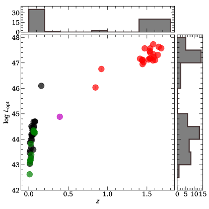
Figure 1: Redshift distribution of the sample as a function of optical luminosity at 5100Å in units of erg s^-1. Black, red, green and magenta symbols correspond to Persson (1988), Martínez-Aldama et al. (2015a, b), Marinello et al. (2016) and Marinello et al. (2020) samples, respectively.

3 Parameter Estimations

3.1 Black hole mass

The black hole mass ($M\mathrm{{}_{BH}}$) is estimated using the classical relation given by:

$$M\mathrm{{}_{BH}}=f\mathrm{{}_{BLR}}\frac{R\mathrm{{}_{BLR}}\,v^{2}}{G}$$ (2)

where $G$ is the gravitational constant, $f\mathrm{{}_{BLR}}$ is the virial factor, $R\mathrm{{}_{BLR}}$ is the broad line region size and $v$ is the velocity field in the BLR, which is represented by the FWHM of H$\beta$. The virial factor includes information of geometry, kinematics, and inclination angle of the BLR. Typically, it is assumed as constant ($\sim 1$), however some results point out that this factor should vary along the AGN populations (e.g. Collin et al., 2006; Yu et al., 2019). In this work, we assume the virial factor proposed by Mejía-Restrepo et al. (2018), which is anti-correlated with the FWHM of the emission line: $f\mathrm{{}_{BLR}}=\left({{\mathrm{FWHM_{H\beta}}}}\,/\,{4550{\pm 1000}}\right)^{-1.17}$.

For single–epoch spectra, the $R\mathrm{{}_{BLR}}$ is usually estimated through the Radius-Luminosity (RL) (Bentz et al., 2013) given by:

$$\mathrm{log}\left(\frac{R\mathrm{{}_{BLR}}}{\mathrm{1lt-day}}\right)= (1.527\,\pm\,0.31)\,+$$

$$\,0.533{{}^{+0.035}_{-0.033}}\,\mathrm{log}\left(\frac{L_{\rm opt}}{10^{44}L_{\odot}}\right).$$ (3)

where $L_{\rm opt}$ corresponds to the luminosity at 5100Å. Black hole mass estimations are reported in Table LABEL:tab:table2. The sample shows a clear distinction between low and high black hole masses (log $M\mathrm{{}_{BH}}$$\sim 7-10$ M_⊙).

3.2 Eddington ratio

The accretion rate is estimated by the classical Eddington ratio defined by $L\mathrm{{}_{bol}}/L\mathrm{{}_{Edd}}$, where $L\mathrm{{}_{bol}}$ is the bolometric luminosity and $L\mathrm{{}_{Edd}}$ is the Eddington luminosity defined by $L\mathrm{{}_{Edd}}=1.5\times 10^{38}\left(\frac{M_{BH}}{M_{\odot}}\right)$. The bolometric luminosity formally can be estimated integrating the area under the broadband spectral energy distribution (SED) (e.g. Richards et al., 2006, and references therein). However, since this process requires multi-wavelength data to constrain the SED fitting process, it is hard to get an estimation for individuals sources. Mean SEDs have been used to estimate average values called bolometric correction factors ($k\mathrm{{}_{bol}}$), which scale the monochromatic luminosity ($\lambda L_{\lambda}$) to give a rough estimation of $L\mathrm{{}_{bol}}$$=k_{\mathrm{bol}}\cdot\lambda L_{\lambda}$. Usually, $k\mathrm{{}_{bol}}$ is taken as a constant for a monochromatic luminosity; however, results like the well-known non-linear relationship between the UV and X-ray luminosities (e.g. Lusso & Risaliti, 2016, and references therein) indicate that $k\mathrm{{}_{bol}}$ should be a function of luminosity (Marconi et al., 2004; Krawczyk et al., 2013). Along the same line, Netzer (2019) proposed new bolometric correction factors as a function of the luminosity assuming an optically thick and geometrically thin accretion disk, over a large range of black hole mass ($10^{7}$- $10^{10}$ M_⊙), Eddington ratios (0.007–0.5), spin (-1–0.998) and a disk inclination angle of $56^{\circ}$. For the optical range, the bolometric correction factor is given by:

$$k_{\mathrm{bol}}=40\left(\frac{L_{\rm opt}}{10^{42}}\right)^{-0.2},$$ (4)

where $L_{\rm opt}$ corresponds to the luminosity at 5100Å. The wide option of parameters considered for the model process provide a better approximation corroborating previous results (Nemmen & Brotherton, 2010; Runnoe et al., 2012a, b). In addition, it provides a better accuracy than the constant bolometric factor correction which led to errors as large as $50\%$ for individual measurements. Therefore, we explore the use of $k\mathrm{{}_{bol}}$ for estimating the Eddington ratio. Table LABEL:tab:table2 reports the Eddington ratios utilizing the BH masses obtained using the classical RL relation (Eq. 3).

4 The correlation analysis

4.1 Observational Pairwise Correlations

Figure 2 shows the correlation matrix of the observational parameters: optical ($L_{\mathrm{opt}}$ at 5100Å) and NIR ($L_{\rm NIR}$ at 8542Å) continuum luminosities, the flux ratios R_FeII and R_CaT and the emission lines properties such as FWHM and the equivalent width (EW) of H$\beta$, O i $\lambda 8446$ and CaT, plus the EW of Fe ii. In order to stress the difference in luminosity and FWHM values in the subsamples, they are identified by different colors. Each panel also includes the Spearman’s rank correlation coefficient ($\rho$) and the $p$-value, where significant correlations ($p<0.001$) are colored in red (otherwise shown in black). Optical and NIR luminosities follow a linear relation (Fig. 2), therefore both luminosities show the same behavior with the rest of the observational properties.

Top panel of Figure 2 shows the strong correlation between R_FeII and R_CaT, which is described by the Eq. 1 (dashed gray line; see also inset panel). The anti-correlation between R_FeII (or R_CaT) and EW_Hβ is expected since the strength of H$\beta$ decreases as R_FeII (or R_CaT) increases. The linear correlation between R_FeII and EW_FeII is due to the fact that both parameters reflects the strength of the Fe ii emission, the first one is weighted by the H$\beta$ flux and the second by the luminosity. It is the same case for the correlation EW_CaT-R_CaT. Since R_CaT is correlated with R_FeII, we expect a positive linear relation between EW_CaT-R_FeII and EW_FeII-R_CaT. On the other hand, R_FeII and R_CaT show non-linear trends with the FWHM of the emission lines, which are further discussed in Section 4.2. The correlation between the EW and the continuum luminosity are extensively described in Sec. 4.3 and 6.2.

The correlations between the FWHM of H$\beta$, O i $\lambda 8446$ and CaT are strongest according to their Spearman coefficients and their associated $p-$values (Fig. 2). In these panels, the 1:1 line is shown for reference. H$\beta$ shows broader profiles than the O i $\lambda 8446$, particularly for the sources with FWHM $>4000$  km s^-1. We obtained the trend lines by least squares (OLS) fitting implemented in python packages sklearn and statsmodels. The relation has a slope of 0.894$\pm$0.05 and a scatter of $\sigma_{\rm rms}\sim$0.115 dex. The deviation at 4000  km s^-1 could be associated with the presence of a red-ward asymmetry in the broadest H$\beta$ profiles, i.e. with an emitting region closer to the continuum source (Marziani et al., 2013; Punsly et al., 2020). The presence of this feature is hard to observe in the O i $\lambda 8446$ profile, since it is blended with the CaT and the NIR Fe ii. On the other hand, CaT is also narrower than H$\beta$, although the scatter is larger ($\sigma_{\rm rms}\sim$0.152 dex) and the relation is slightly shallower than the one given by O i $\lambda 8446$ with a slope of 0.827$\pm$0.08. O i $\lambda 8446$ and Ca ii show similar widths, the predicted relation gives a slope of 0.944$\pm$0.05 and the scatter is smaller ($\sigma_{\rm rms}\sim$ 0.103 dex) than in the previous cases. This general behavior corroborates that H$\beta$ is emitted closer to the continuum source than O i $\lambda 8446$ and CaT (Persson, 1988; Martínez-Aldama et al., 2015a; Marinello et al., 2016).

4.2 Eigenvector 1 sequence

The correlation between R_FeII and the FWHM of H$\beta$ is known as the Eigenvector 1 (EV1) sequence (Boroson & Green, 1992), which is also known as the quasar main sequence (Sulentic et al., 2000). According to the EV1 scheme, the observational and physical properties of type 1 AGN change along the sequence (Marziani et al., 2018; Panda et al., 2018, 2019). Based on the R_FeII strength the accretion rate can be inferred, where the sources with R_FeII$>$1 are typically associated with the highest Eddington ratios ($L\mathrm{{}_{bol}}/L\mathrm{{}_{Edd}}$$>$0.2, Marziani et al., 2003; Panda et al., 2019, 2020b). The relation between these parameters is not linear (Wildy et al., 2019), where orientation and luminosity are also involved (Shen & Ho, 2014; Negrete et al., 2018)

The EV1 sequence (FWHM_Hβ-R_FeII  relation) of our sample is shown in Figure 2. A displacement between the low– and high–luminosity objects (HE sample) can be appreciated, however, both kinds of sources follow the same trend. This displacement is only a luminosity effect, where the HE sample is shifted to the larger FWHM values of the panel. An EV1-like sequence is also appreciated in the relations R_FeII-FWHM_CaT and R_FeII-FWHM_OI,which is expected due to the linear relation between the widths of the emission lines (Sec. 4.1).

The relation FWHM_Hβ-R_CaT shows an EV1 sequence-like for the low-luminosity subsample, but it is not appreciated in the high luminosity objects, the HE sample. It seems that in some objects the CaT increases with increasing FWHM_Hβ. The same effect is observed for the relations FWHM_OI-R_CaT and FWHM_CaT-R_CaT. Surprisingly, the break occurs at R_CaT$\sim 0.2$ which corresponds to R_FeII=1 (following the Eq. 1), the limit for the highly accreting sources according to Marziani et al. (2003). A similar decoupling is also observed in the relation between the EW_CaT and the FWHM of the emission lines, but the scatter is quite large. Martínez-Aldama et al. (2015a) found a rough enhancement of EW_CaT for the HE sample at intermediate–$z$ with respect to the other objects at low-$z$ attributing this behavior to a burst of star formation and an enrichment at intermediate redshift sources. The new HE objects (Martínez-Aldama et al., 2015b) added to the presented analysis seem to corroborate these results, however, some selection effect could also be involved. We discuss this result in Sec. 6.3.

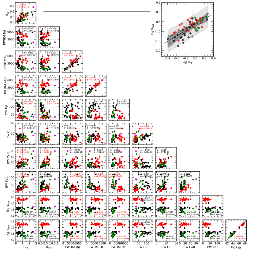
Figure 2: Correlation matrix for emission lines and continuum properties. Black, red, green and magenta symbols correspond to Persson (1988), Martínez-Aldama et al. (2015a, b), Marinello et al. (2016) and Marinello et al. (2020) samples, respectively. Each panel specifies the Spearman’s rank correlation coefficient and the $p-$value, where the significant correlations are colored in red. Equivalent width (EW), FWHM, optical and NIR luminosities are given in units of Å,  km s^-1 and erg s^-1, respectively. Gray vertical-lines in the first column mark the limit for super-Eddington sources at R_FeII=1.0. In the diagrams where the FWHMs and luminosities are correlated, the gray dashed line marks the relation 1:1. In the correlation R_CaT-R_FeII  gray dashed line corresponds to Eq. (1). The inset right panel shows the relation R_FeII-R_CaT in log–scale with the results of the bootstrap analysis, see Sec. 4.5. Black dotted lines mark the confidence intervals at 95% for the 1000 realizations (dark gray lines) of the bootstrap analysis. Lightgray patch marks the corresponding prediction intervals bands for the sample.

4.3 Correlations with the equivalent width: the Baldwin effect

The anti-correlation between the equivalent width and the luminosity is known as the global Baldwin effect (BEff) (Osmer & Shields, 1999; Green et al., 2001; Baskin & Laor, 2004; Bachev et al., 2004; Dong et al., 2009; Zamfir et al., 2010), which was first observed between the equivalent width of C iv$\lambda 1549$ and the continuum luminosity at 1450Å (Baldwin, 1977). The BEff is clearly appreciated in the high–ionization lines, except NV $\lambda 1240$ due to a second enrichment (Osmer et al., 1994). However, as the ionization potential decreases the slope of this anti-correlation gets shallower and it is hard to distinguish a strong correlation for low-ionization lines (Sulentic et al., 2000; Dietrich et al., 2002) An intrinsic Baldwin effect (Pogge & Peterson, 1992) has been also detected in the multi-epoch observations for single variable AGNs. The BEff provides information about the ionizing continuum shape (Wandel, 1999), structure, and metallicity (Korista et al., 1998) of the BLR. Also, it has been used for calibrating the luminosity in cosmological studies (Baldwin et al., 1978; Korista et al., 1998).

4.3.1 Luminosity

Figure 3 shows the equivalent widths of H$\beta$, O i $\lambda 8446$, optical Fe ii and CaT as a function of the optical and NIR luminosities. Spearman rank correlation coefficients, $p-$values and the scatter of the correlations are reported in Table LABEL:tab:params_corr. None of the trends between the EW and the optical and NIR luminosity satisfies the criteria for a significant relation and all of them show shallow relations with a slope of $\alpha<0.1$. The shallow slope confirms the weak relation between the luminosity and the EW for low ionization lines. This result is in agreement with larger samples at high redshift (Dietrich et al., 2002). The negative correlation between EW_Hβ and $L_{\rm opt}$ ($\alpha=-0.064\pm 0.032,\,\rho=-0.412$, $p=0.001$) is expected due to the behavior of individual variable sources (e.g. Rakić et al., 2017). This behavior is different from the one of the relation EW_CaT-$L_{\mathrm{opt}}$  ($\alpha=0.068\pm 0.053$, $\rho$=0.417 $p=0.001$), which suggests the presence of an inverse Baldwin effect. A positive correlation has also been observed between the continuum at 5100Å and the optical Fe ii in the monitoring of the variable NLSy1 NGC 4051 (Wang et al., 2005). The strong correlation between the Fe ii and CaT explain this behavior. However, in our sample the relation EW_FeII-$L_{\mathrm{opt}}$ is negative ($\alpha=-0.091\pm 0.039$, $\rho=-0.409,\,p=0.001$) and is just below the criteria assumed to consider a significant correlation. Other studies neither reported a BEff for optical nor for UV Fe ii  (Dong et al., 2011). Finally, the trend observed for EW_OI-$L_{\mathrm{opt}}$ is not significant and show a slope consistent with zero ($\alpha=-0.007\pm 0.034$), also confirmed by previous studies (Dietrich et al., 2002).

4.3.2 Black hole mass and Eddington ratio

Since the black hole mass and the Eddington ratio have been considered as the main drivers of the BEff (Wandel, 1999; Dong et al., 2011), we also present the correlations EW-$M\mathrm{{}_{BH}}$ and EW-$L\mathrm{{}_{bol}}/L\mathrm{{}_{Edd}}$ in Fig. 3. The parameters of the correlations are reported in Table LABEL:tab:params_corr. The only significant relation involving the black hole mass is EW_FeII-$M\mathrm{{}_{BH}}$  ($\rho=-0.493$, $\alpha=-0.151\pm 0.060$ $\sigma_{\rm rms}\sim 0.234$ dex).

In the correlations between the equivalent width and the Eddington ratio, the significant relations are the ones involving EW_Hβ and EW_CaT. In both cases the correlations are sharper ($\alpha_{\rm H\beta}=-0.332\pm 0.149$, $\alpha_{\rm CaT}=0.428\pm 0.237$) and stronger ($\rho_{\rm H\beta}=0.531$, $\rho_{\rm CaT}=0.482$) than the luminosity case. Although the correlations for Fe ii and O i $\lambda 8446$ are below the significance level, their slopes are steeper than the correlations with respect to the luminosities and the black hole mass. Hence, the Eddington ratio highlights the correlations with the equivalent width, as Baskin & Laor (2004) and Dong et al. (2011) previously reported.

Figure 3: Correlation matrix for the optical and NIR luminosities, black hole and the equivalent width of H$\beta$, optical Fe ii, O i $\lambda 8446$ and CaT. Green and blue symbols indicate the low– and high–luminosity subsamples, respectively (Sec 4.3.3). Black dashed line represents the best OLS fitting for the full sample. The Spearman’s rank correlation coefficient, $p-$values, slope ($\alpha$), and scatter ($\sigma_{\rm rms}$) are also shown, where the significant correlations are colored in red. Black dotted lines mark the confidence intervals at 95% for the 1000 realizations (dark gray lines) of the bootstrap analysis. Lightgray patch marks the corresponding prediction intervals bands for the sample.

4.3.3 Division of the sample

According to Dietrich et al. (2002) to avoid selection effects in the global BEff a sample with a wide luminosity range is needed, $42<{\rm log}\,L<48$. Our sample covers this range, however at high redshift only high luminosity sources are available (${\rm log}\,L_{\rm opt}>47.5$ erg s^-1). In order to clarify the results of Sec. 4.3 and the presence of possible bias, we divided the sample into two subsamples considering the median luminosity, log $L_{\rm opt}=44.49$ erg s^-1. In Fig. 3 the low– and high–luminosity subsamples are represented by green and blue symbols, respectively. The division of the sample directly affects the relations EW$-L_{\rm opt}$, EW$-L_{\rm NIR}$ and EW$-{\rm M}_{\rm BH}$ where no significant correlations are observed, which also reflects the bias involved in this consideration. For example, the relation EW_Hβ$-L_{\rm opt}$ is positive for the low-luminosity subsample ($\alpha=0.1\pm 0.073$, $\rho=0.235$, $p=0.281$), while for the the high luminosity case the relation has a different direction ($\alpha=-0.13\pm 0.031$, $\rho=-0.53$, $p=0.003$), similar to the behavior of the full sample. The difference in the subsamples is also pointed out by the PCA (Appendix D). Therefore, the correlations have some relevance only when the full sample is considered .

However, the correlations EW–$L\mathrm{{}_{bol}}/L\mathrm{{}_{Edd}}$ are less affected by the division of the sample, at least, in the significant correlations provided by the full sample analysis. In the relation EW_Hβ–$L\mathrm{{}_{bol}}/L\mathrm{{}_{Edd}}$, the direction of the best fits in the subsamples is still negative ($\alpha_{\rm low}=-0.215\pm 0.162,\alpha_{\rm high}=-0.472\pm 0.144$), although none of the relations are significant ($\rho_{\rm low}=-0.26,\,p_{\rm low}=0.181,\,\rho_{\rm high}=-0.35,\,p_{\rm high}=0.07$). While in the EW_CaT–$L\mathrm{{}_{bol}}/L\mathrm{{}_{Edd}}$ relation, the slope for the subsamples is positive ($\alpha_{\rm low}=0.240\pm 0.158,\,\alpha_{\rm high}=0.694\pm 0.242$) such as in the full sample, but without any significance ($\rho_{\rm low}=0.222,\,p_{\rm low}=0.245,\,\rho_{\rm high}=0.313,\,p_{\rm high}=0.098$). This result suggests that $L\mathrm{{}_{bol}}/L\mathrm{{}_{Edd}}$ is less influenced by a bias and it then regulates the correlation between the equivalent width and the luminosity, as originally suggested by Baskin & Laor (2004) and Bachev et al. (2004).

4.4 The behavior of R_FeII, R_CaT and the ratio Fe ii/CaT

Fig. 4 shows the behavior of R_FeII, R_CaT and the ratio Fe ii/CaT as a function of optical and NIR luminosity, black hole mass and Eddington ratio. R_FeII and R_CaT do not show any significant correlation with the luminosity and black hole mass for the full sample. Only the Fe ii/CaT  shows a significant anti-correlation with the optical ($\rho=-0.441,\,p=5.3\times 10^{-4}$) and NIR luminosity ($\rho=-0.456,\,p=3.2\times 10^{-4}$). If the subsamples are considered, all the best fits are below the statistical significance limit.

In the panels where $L\mathrm{{}_{bol}}/L\mathrm{{}_{Edd}}$ is involved, the strongest correlation is the one corresponding to the ratio Fe ii/CaT ($\rho=0.554$, $p=6.4\times 10^{-6}$), followed by the one with R_CaT ($\rho=$0.425, $p=8.9\times 10^{-4}$). In both cases the trend lines for the full samples and subsamples have the same direction such as in Fig. 3, although the significant correlation arises only for the full sample.

The positive correlation between R_CaT and $L\mathrm{{}_{bol}}/L\mathrm{{}_{Edd}}$ confirm that the strength of CaT is driven by the accretion rate, and it remains even after the division of the sample. Although the same behavior is expected for R_FeII, we cannot confirm this result in our sample. The positive correlation between the optical and UV R_FeII and $L\mathrm{{}_{bol}}/L\mathrm{{}_{Edd}}$ is robust (e.g Zamfir et al., 2010; Dong et al., 2011; Martínez-Aldama et al., 2020). Besides, the R_FeII has been used as a proxy for the $L\mathrm{{}_{bol}}/L\mathrm{{}_{Edd}}$ to correct the time delay by the accretion effect and decrease the scatter in the optical and UV Radius-Luminosity relation (Du & Wang, 2019; Martínez-Aldama et al., 2020). This indicates that the Fe ii (and R_FeII) in our sample is affected by several factors: the sample size, the quality of the observations and the Fe ii templates employed, which could decrease the accuracy of its estimation. For instance, 10 objects from the Persson (1988) sample have only upper limits, such as Mrk 335. It is one of the five common sources observed by Marinello et al. (2016), where the R_FeII value is $\sim 50\%$ higher than the value estimated by Persson (1988). It confirms that the objects with upper values are highly inaccurate and thus it could be reflected in the loss of the correlation with other parameters. A homogeneous fitting process considering the same analysis spectral procedure could help to decrease the scatter and clarify the trends which we aim to pursue in a future work.

4.5 Bootstrap analysis

4.5.1 Random distributions

Which is the probability that an uncorrelated data set gives a correlation with Spearman rank coefficient as high as the one we observe? In order to answer this question, we modeled the distributions of each of the parameters in Fig. 3 and 4 considering a random sample of 1000 elements and the probability distributions implemented in the module stats in python. To determine how good of a fit this distribution is, we used the Kolmogorov-Smirnov test which compare a sample with a reference probability distribution and we chose the distribution with the highest $p-$value_ran. Since the luminosity and the black hole mass show bimodal distributions, we used two distributions to reproduce the observational one. In the rest of the cases a good fit was obtained with only one distribution. The probability distributions considered and the $p-$value are reported in column (11) and (12) of Table LABEL:tab:params_corr. The distribution fitting of the correlation $L\mathrm{{}_{bol}}/L\mathrm{{}_{Edd}}$-Fe ii/CaT is shown in Fig. B.1 as an example of this analysis.

Later, we randomly selected 58 realizations from the original 1000, which later we correlated following the correlations in Figures 3 and 4, and in the correlation R_FeII-R_CaT. Finally, we repeated the process 2000 times and estimated the Spearman rank correlation coefficient ($\rho_{\rm ran}$), the corresponding $p-$value and estimated the fractions of significant correlations ($f_{\rm ran}$). Results are reported in column (13) of Table LABEL:tab:params_corr. In all the cases $f_{\rm ran}<1\times 10^{-3}$, it means that is very unlikely at $3\sigma$ confidence level that two independent correlations provide high correlations coefficients such as the observational sample does. Therefore, our analysis supports the reliability of the observed correlations.

4.5.2 Linear regression fitting

Due to the small size of our sample and the gaps in luminosity and redshift, we proved the statistical reliability of the correlations in Fig. 3 and 4 via a bootstrap analysis (Efron & Tibshirani, 1993). The bootstrap sample is formed by the selection of a subset of pairs from each one of the correlations by random resampling with replacement. We created 1000 realizations and then performed a linear regression fitting. The gray lines in Fig. 2 and 3 correspond to the 1000 realizations, which are in agreement with the best fit of each correlation at 2$\sigma$ confidence level (dotted black lines). As a reference, the figures also shows the prediction intervals bands (lightgray patch), which indicate the variation of the individuals measurements and predict that 95$\%$ of the individual point lies within the patch. As a reference, we also analyzed the relation R_FeII-R_FeII (inset panel, Fig. 2) to compare the behavior of the bootstrap analysis in a very well-know correlation, obtaining an agreement within $2\sigma$ confidence level.

In order to quantify the bootstrap results, we considered the percentiles at $2\sigma$ confidence level and estimated the errors of the slope ($\alpha_{\rm BS}$) and ordinate ($\beta_{\rm BS}$) of the normal distribution drawn from the 1000 realizations for each correlation. Results are reported in Table LABEL:tab:params_corr. As it is expected the distributions are centered in the slope and ordinates values of each correlations, which are completely equivalent to the ones from the observational correlations. The magnitude of the errors indicates the reliability of the correlation. The larger errors are associated with the correlations below the significance criteria ($-0.4<\rho_{\rm BS}<0.4$, $p>0.001$). A clear example are the errors in the slope of the relations involving O i $\lambda 8446$ (Fig. 3) or R_FeII (Fig. 4), which indicates the inaccuracy of the results, such as the Spearman correlation coefficient shows. Meanwhile, good correlations, such as R_FeII-R_CaT, will show errors $<20\%$. As the correlation coefficients indicate, the errors decrease considerably in the correlations where $L\mathrm{{}_{bol}}/L\mathrm{{}_{Edd}}$ is involved. This result points out the relevance of $L\mathrm{{}_{bol}}/L\mathrm{{}_{Edd}}$ in the behavior of our sample and its role in the Baldwin effect.

On the other hand, we also estimated the Spearman correlation coefficient (${\rho_{\rm BS}}$) for the 1000 realizations and estimated the fraction of significant realizations respect to the total number ($f_{\rm sig}$), which satisfy the significance criteria ($|\rho|>0.4$ and $p<0.001$). We also modeled the distribution of ${\rho_{\rm BS}}$ using a skewnorm distribution and estimated the error at $2\sigma$ confidence level. The maximum of the ${\rho_{\rm BS}}$ distribution and $f_{\rm sig}$ are reported in columns (9) and (10) of Table LABEL:tab:params_corr. In the strongest correlation of the sample, R_FeII-R_CaT, we obtained $f_{\rm sig}$=1. It means that the 1000 bootstrap realizations satisfy the significant criteria and confirm the reliability of the correlation. This is also highlighted by the errors of ${\rho_{\rm BS}}$, where the correlation remains significant within the uncertainty range. In the correlations with $|\rho_{\rm BS}|>0.5$, $f_{\rm sig}>0.75$ indicating a reliable correlations. However, if the errors of ${\rho_{\rm BS}}$ are considered, there is an small possibility to dismiss the significance of the correlation. It can be expressed by the parameter 1-$f_{\rm sig}$, which expresses the probability of failing to detect a correlation. Thus, there is probability of $<25\%$ to detect a false positive correlation in EW_Hβ–$L\mathrm{{}_{bol}}/L\mathrm{{}_{Edd}}$ and Fe ii/CaT–$L\mathrm{{}_{bol}}/L\mathrm{{}_{Edd}}$. If $|\rho_{\rm BS}|=0.4-0.5$, great care should be considered because the probability to detect a false positive correlation increases to $(1-f_{\rm sig})\sim 50\%$. It is the case of the correlations such as EW_CaT-$L\mathrm{{}_{bol}}/L\mathrm{{}_{Edd}}$ or Fe ii/CaT-$L_{\rm opt}$. The same interpretation of false positive probability applies in the case of no detected correlation in the observed or bootstrap samples ($\rho<0.4$), when the probabilities are always low, particularly for the weakest correlations $(1-f_{\rm sig}>80\%)$.

4.6 Residuals behavior

In order to assess a possible redshift effect in our results, we estimated the residuals with respect to the best fit for the correlations in Fig. 3 and Fig. 4. We divided the sample into low– and high–$L$ subsamples, which is equivalent to a division into low– and high–redshift. The behavior of the distributions is shown in Fig. B.2 and B.3. If any significant difference of the median of the distribution with respect to the zero residual level is observed, it could indicated a redshift effect. In all the correlations of Fig. B.2, we observed a difference within $2\sigma$ confidence level. On the other hand, the relations of Fig. 4 show the same behavior, however the width of the distribution increases significantly as well as the median values, particularly for the correlations involving R_FeII. Since this behavior is only observed in these correlations and they still show a dependency within $2\sigma$ level, we cannot claim a redshift effect. As we mentioned previously, the R_FeII is not well behaved in our sample compared to previous results. Therefore any trend involving R_FeII must be taken with caution.

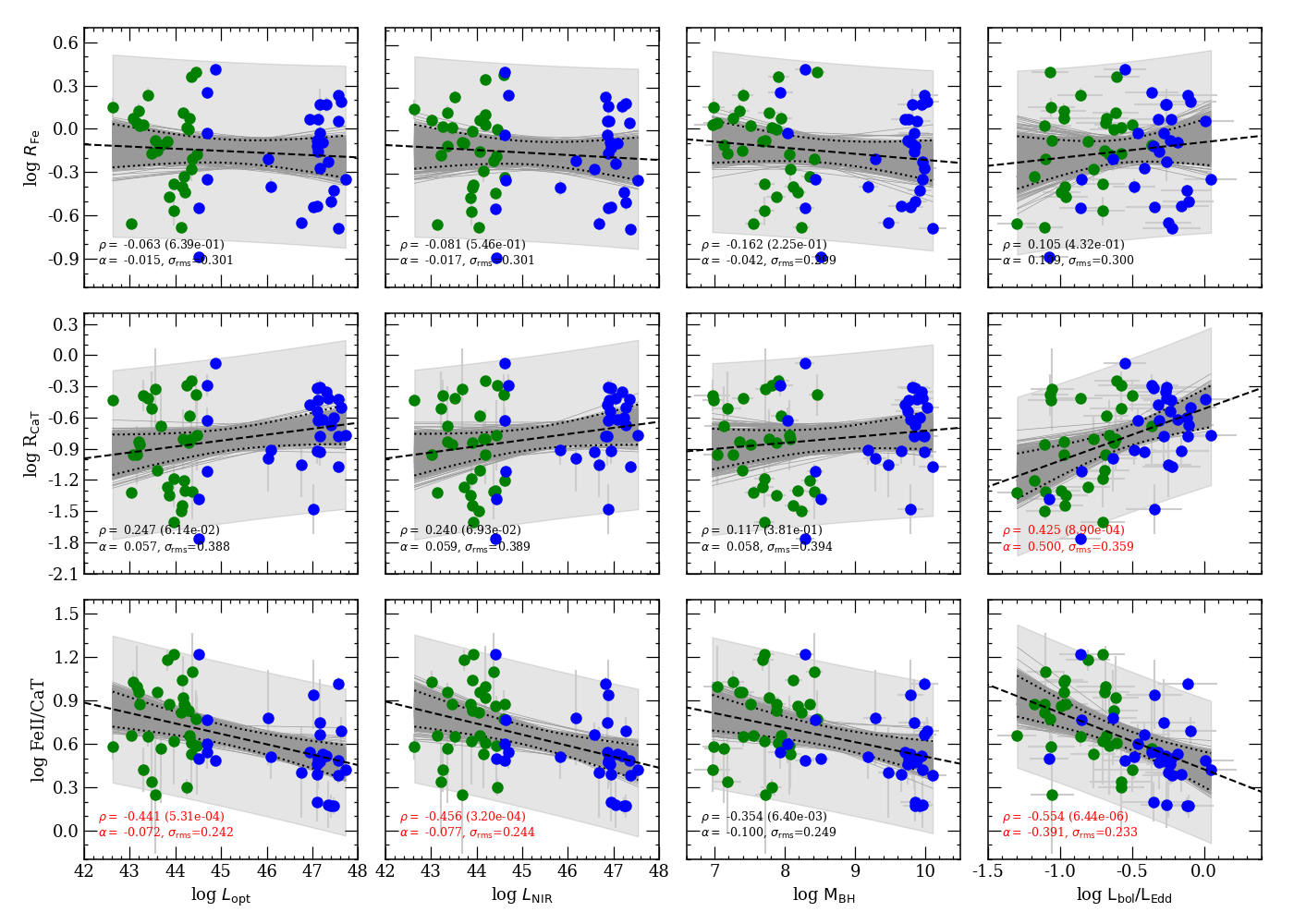
Figure 4: Correlation matrix for optical and NIR luminosity, black hole mass, Eddington ratio ($L\mathrm{{}_{bol}}/L\mathrm{{}_{Edd}}$), R_FeII, R_CaT and Fe ii/CaT ratio. Colors and symbols are the same as Fig.3.

5 Principal Component analysis

Principal component analysis (hereafter PCA) allows to get a better view of the data where it can be separated in a quantitative manner, such that the relevant properties explain the maximum amount of variability in the dataset. PCA works by initially finding the principal axis along which the variance in the multidimensional space (corresponding to all recorded properties) is maximized. This axis is known as eigenvector 1. Subsequent orthogonal eigenvectors, in order of decreasing variance along their respective directions, are found, until the entire parameter space is spanned (see, for example, Boroson & Green, 1992; Kuraszkiewicz et al., 2009; Wildy et al., 2019; Tripathi et al., 2020). The PCA method is particularly useful when the variables within the data set are highly correlated. Correlation indicates that there is redundancy in the data. Due to this redundancy, PCA can be used to reduce the original variables into a smaller number of new variables (principal components) explaining most of the variance in the original variables. This allows to determine correlated parameters and, in the context of our work, we utilize this technique to determine the physical parameter(s) that lead to the correlations illustrated in Fig. 3 and 4.

Eigenvalues (or loadings) can be used to determine the numbered principal components to retain after PCA (Kaiser, 1961): (a) An eigenvalue $>$ 1 indicates that principal components (PCs) account for more variance than accounted by one of the original variables in standardized data. This is commonly used as a cutoff point for which PCs are retained. This holds true only when the data are standardized, i.e., they are scaled to have standard deviation one and mean zero; and (b) one can also limit the number of component that accounts for a certain fraction of the total variance. Since there is no well-accepted way to decide how many principal components are enough, in this work we evaluate this using the scree plot (see, for example, Figure 5), which is the plot of eigenvalues ordered from largest to the smallest. A scree plot shows the variances (in percentages) against the numbered principal component, and allows visualizing the number of significant principal components in the data. The number of components is determined at the point beyond which the remaining eigenvalues are all relatively small and of comparable size (Peres-Neto et al., 2005; Jolliffe, 2011). This helps to realize whether the given data set is governed by a single or more-dimensions, where a dimension refers to a variable. Subsequently, these principal components are investigated against the original variables of the dataset to extract information of the importance of these variables in each principal component.

We consider the 58 sources in our sample and collect the properties that are common among them. Due to the diversity in the studied subsamples, we only have 12 parameters that are obtained/estimated directly from the observation: $z$, optical and NIR luminosity, R_FeII, R_CaT, FWHM and EW of H$\beta$, O i $\lambda 8446$ and CaT, as well as the EW of Fe ii. Among these 12 parameters, the redshift and the optical luminosities are correlated by a bias effect as shown in Figure 1 and hence we drop the redshift and only choose the optical luminosity. Thus we have a 11 parameters that are considered in the initial PCA. Later, we only adopt the NIR luminosity which is equivalent to the optical (Fig. 2). We refer the readers to Appendix C for more details on the initial PCA tests, a note on the effect redundant parameters play in this analysis and the final set of parameters used to infer the observed correlations.

Next, we have the derived parameters - bolometric luminosity ($L\mathrm{{}_{bol}}$), black hole mass ($M\mathrm{{}_{BH}}$) and Eddington ratio ($L\mathrm{{}_{bol}}/L\mathrm{{}_{Edd}}$), which are predicted using one or more of the observed parameters that are already taken into account for the PCA run. PCA is an orthogonal linear transformation technique applied to the data and assumes that the input data contains linearly independent variables such that the eigenvectors can be represented as a sum of linear combination of variables with associated weights (eigenvalues or loadings) corresponding to each variable. Thus, in order to remove any redundancy in the result obtained via the PCA, one needs to make sure that the parameters that go in as input are not scaled up version of another parameter, thereby saving us the trouble of unwanted bias that comes out of it. The effect of the inclusion of derived variables in the PCA is illustrated in Appendix C.

Similar to Wildy et al. (2019), we use the prcomp module in the R statistical programming software. In addition to prcomp, we use the factoextra package for visualizing the multivariate data at hand, especially to extract and visualize the eigenvalues/variances of dimensions.

5.1 PCA on the full sample

The tests aimed to reduce the redundancy of the variables were applied as described in (see appendix C) and now allow us to perform a final PCA run with the dataset that contain variables which are obtained directly from the observations and have as little redundancy as possible. The final input contains 8 variables, namely, the NIR luminosity (at 8542 Å), the EWs of Fe ii, H$\beta$, O i $\lambda 8446$ and CaT, and, the FWHMs of H$\beta$, O i $\lambda 8446$ and CaT. The result of the PCA is illustrated in Figure 5.

In this section, we present the results of the PCA on the full sample and infer the relative importance of the eigenvectors as a function of the input variables. In Appendix D is described the PCA analysis for the low- and high-luminosities samples described in Sec. 4.3.3. Figure 5 shows the two-dimensional factor-map between the first two principal components, scree plot and the contributions of the input variables to the first four principal components for the full sample. The factor-map shows the distribution of the full sample categorically colored to highlight the different sources (see Sec. 2) in the eigen-space represented by the two principal components, Dim-1 and Dim-2 (i.e., the PC1 and PC2). The first and the second PC contribute 40.6% and 22.2% to the overall dispersion in the dataset. Combining the contributions from the two subsequent PCs (PC3 and PC4), one can explain 89.1% of the variation present in the data. We demonstrate the contributions of the original variables on these four principal components to draw conclusions on the primary driver(s) of the dataset.

First principal component: From the factor-map we find that the vectors corresponding to the FWHMs of H$\beta$, O i $\lambda 8446$, CaT and the NIR luminosity are nearly co-aligned, with the FWHM vectors of H$\beta$ and O i $\lambda 8446$ having almost similar orientation. These four vectors are also the major contributors to the variance along the primary principal component (see third panel on the left of Figure 5). The red dashed line on the graph above indicates the expected average contribution. If the contribution of the variables were uniform, the expected value would be 1/length(variables) = 1/8 $\approx$ 12.5%. For a given component, a variable with a contribution larger than this cutoff could be considered as important in contributing to the component. The EW_FeII is barely over this cutoff limit.

Second principal component: The factor-map highlights the prevalence of the EW_CaT which contributes $\sim$45% to this component, followed by the EW_OI and EW_FeII. The overall contribution accounts for $\sim$95% from these three variables.

Third and fourth principal components: The third PC is dominated by the EW_Hβ with a minor contribution from FWHM_Hβ, EW_OI and FWHM_OI. Whereas, the fourth PC is singularly governed by NIR luminosity. The other variables are below the expected average contribution limit.

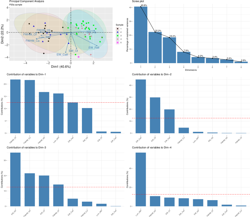
Figure 5: Graphical representation (factor-map) of the principal component analysis (PCA) decomposition of our sample (58 sources) is shown in the first panel. The dots represent individual objects on the standardized PC1 - PC2 plane that have variables indicated by the axis labels. The arrows represent the prominence of the variables in the PC1 - PC2 plane. The dashed lines mark the coordinate axes in the PC1 - PC2 plane and the ellipses depict the 95% occupancy of the sources in their respective subsamples. The sample is categorized based on their original source catalogues (see Panda et al., 2020a, for details on the observational sample) - (1) Martínez-Aldama et al. (2015a); (2) Martínez-Aldama et al. (2015b); (3) Persson (1988); (4) Marinello et al. (2016); and (5) PHL1092 (Marinello et al., 2020). The other panels illustrate the precedence of the first 10 principal components in the form of scree plots, followed by the contributions of the original variables to the first four principal components.

5.2 Correlations between the principal eigenvectors and observed/derived parameters

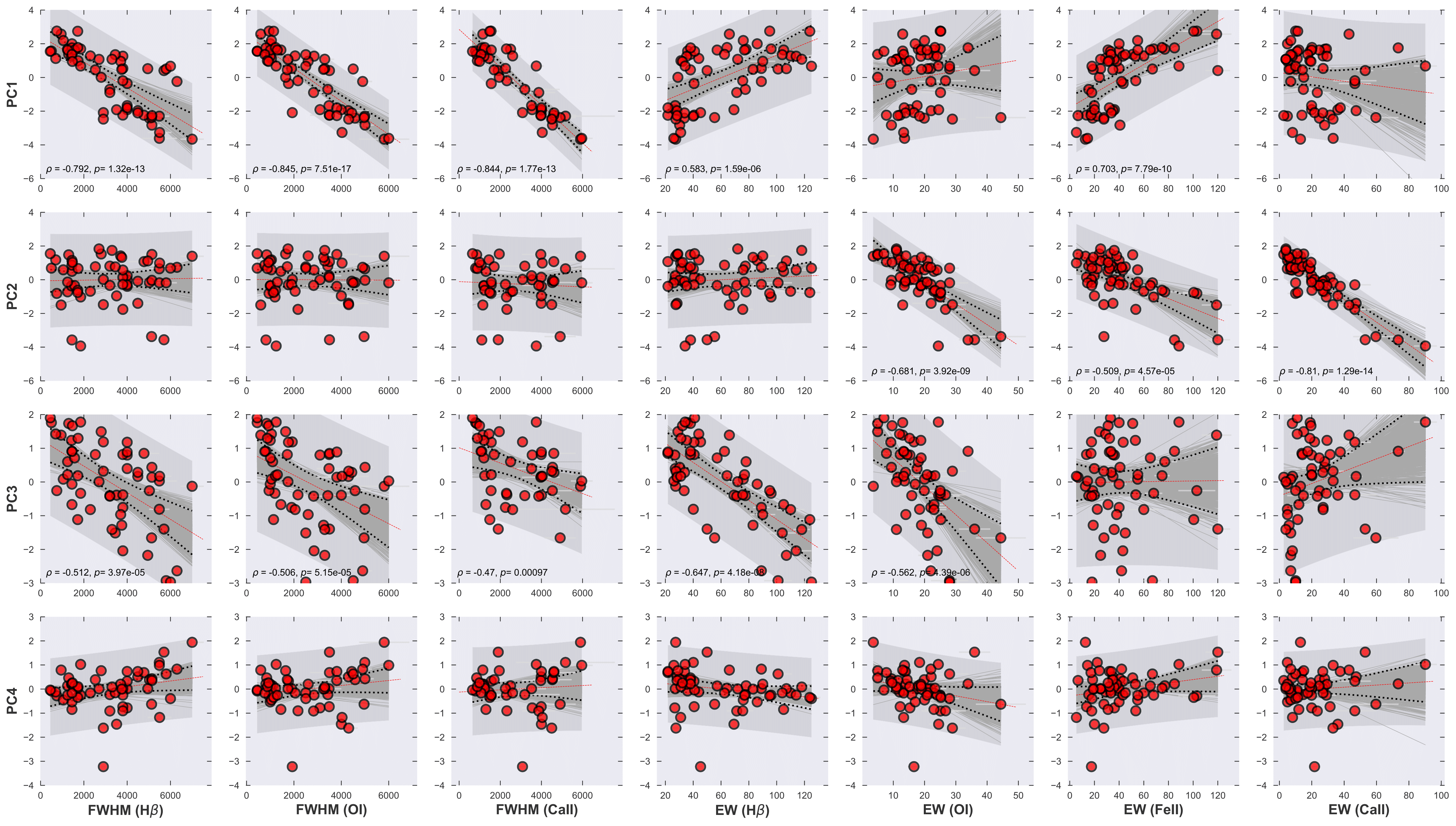
Figure 6: Correlation matrix showing dependence of the first four PCA vectors’ loadings versus the physical parameters (observed) for our full sample. The Spearman’s rank correlation coefficient ($\rho$) and the $p-$value are reported for the correlations whenever $p$-value $<$ 0.001. The OLS fits in each panel are shown with red dashed lines. Black dotted lines mark the confidence intervals at 95% for the 1000 realizations (dark gray lines) of the bootstrap analysis. Lightgray patch marks the corresponding prediction intervals bands for the sample.

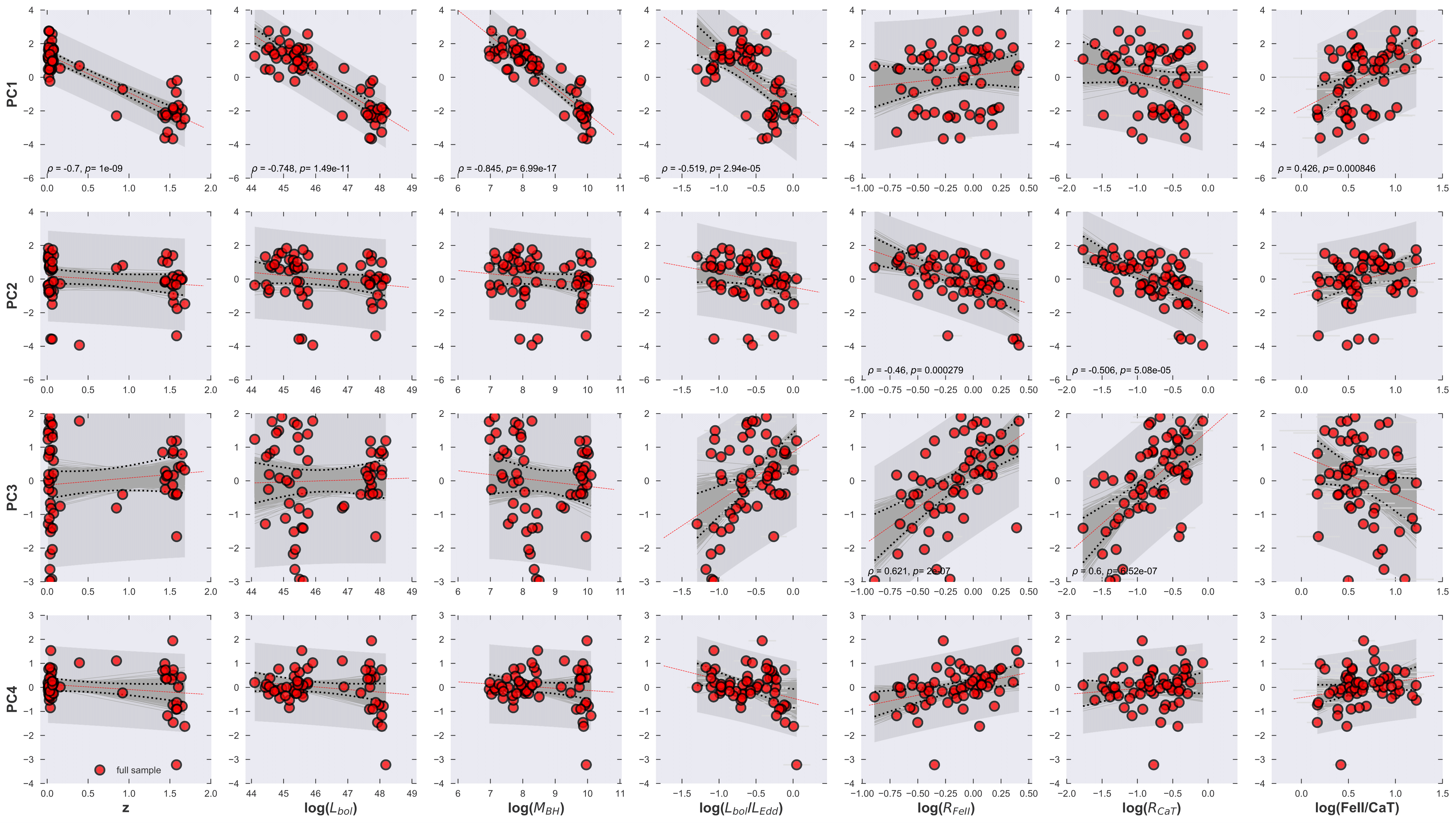
Figure 7: Correlation matrix showing dependence of the first four PCA vectors’ loadings versus the physical parameters (derived) for our full sample. The Spearman’s rank correlation coefficients ($\rho$) and the $p-$values are reported for the correlations whenever $p-$value $<$ 0.001. The OLS fits in each panel are shown with red dashed lines. Black dotted lines mark the confidence intervals at 95% for the 1000 realizations (dark gray lines) of the bootstrap analysis. Lightgray patch marks the corresponding prediction intervals bands for the sample.

To quantitatively assess the relevance of the observational variables and the derived physical parameters we show their correlation against the contributions (loadings) of the the first four principal components (PC1, PC2, PC3 and PC4) for the full sample in Figures 6 and 7. The full-sample is then separated into two subsamples based on the median optical luminosity of the full-sample (i.e. log $L_{\mathrm{opt}}$ = 44.49 erg s^-1). A comparative analysis of the full-sample against the two subsamples is carried out in Appendix D and in Figures D.2 and D.3.

Figure 6 is basically the correlation matrix representation for the Figure 6 that includes all the intrinsic variables (except for the NIR luminosity). We only state the values of the Spearman’s correlation coefficient and the corresponding $p$-value when the correlation is significant ($p<$ 0.001). In the full sample, the strongest correlation with respect to PC1 (in decreasing order) are exhibited by FWHM_OI ($\rho$=-0.845, $p$=7.51$\times 10^{-17}$), FWHM_CaT ($\rho$=-0.844, $p$=1.77$\times 10^{-13}$), FWHM_Hβ ($\rho$=-0.792, $p$=1.32$\times 10^{-13}$), EW_FeII ($\rho$=0.703, $p$=7.79$\times 10^{-10}$), and by EW_Hβ ($\rho$=0.583, $p$=1.59$\times 10^{-6}$). In case of PC2, significant correlations are obtained only for the EWs of CaT ($\rho$=-0.81, $p$=1.29$\times 10^{-14}$), O i $\lambda 8446$ ($\rho$=-0.681, $p$=3.92$\times 10^{-9}$) and Fe ii ($\rho$=-0.509, $p$=4.57$\times 10^{-5}$). For the PC3, there are negative correlations right above the significance limit for the three FWHMs and the EWs for H$\beta$ and O i $\lambda 8446$. The correlations for the subsamples are described in Appendix D.

Figure D.3 corresponds to the derived parameters - bolometric luminosity, black hole mass, Eddington ratio, R_FeII, R_CaT and the ratio of the two species, Fe ii/CaT. For the full sample, we see clear, strong anti-correlations with PC1 for the black hole mass ($\rho$=-0.845, $p$=6.99$\times 10^{-17}$), the bolometric luminosity ($\rho$=-0.748, $p$=1.49$\times 10^{-11}$), followed by the redshift ($\rho$=-0.7, $p$=1$\times 10^{-9}$) and Eddington ratio ($\rho$=-0.519, $p$=2.94$\times 10^{-5}$). Although, in the case of the correlation with respect to the redshift, this is biased due to the gaps in the sample distribution which is highlighted in the panels in the left column (this is also illustrated in Figure 1). For the remaining trends, they corroborate with the correlations that were obtained with the FWHMs in the previous figure. We also see a mild positive correlation of the PC1 with the ratio, Fe ii/CaT ($\rho$=0.426, $p$=8.46$\times 10^{-4}$). There are only two significant correlations obtained with respect to PC2, i.e. for the two line ratios - R_CaT ($\rho$=-0.506, $p$=5.08$\times 10^{-5}$) and R_FeII ($\rho$=-0.46, $p$=2.79$\times 10^{-4}$). This checks the observed correlation that is obtained and studied in this work and in our previous studies. The correlations with PC3 and the two ratios - R_FeII ($\rho$=0.621, $p$=2$\times 10^{-7}$) and R_CaT ($\rho$=0.6, $p$=1.52$\times 10^{-7}$) indicates that the R_FeII-R_CaT correlation in the full dataset is at least two dimensional and may have multiple drivers for this observed correlation. Following the same analysis carried out in Sec. 4.5, we also performed a bootstrap analysis for the correlations in Fig. 6 and 7 which reflects the behavior observed in Sec. 4.5. The correlations for the subsamples are described in Appendix D.

6 Discussion

In this paper, we carefully look at the observational correlations from the up-to-date optical and near-infrared measurements centered around Fe ii and CaT emission, respectively. Since our sample is affected by bias, we explored its influence in our results, showing that the correlations with the Eddington ratio and the independent observational parameters are less biased than the ones involving luminosity or black hole mass. These results are supported by a bootstrap analysis, which corroborated the statistical meaning of the correlations. We did not detect any redshift dependence in the correlations with luminosity and Eddington above 2$\sigma$ confidence level. We also performed a Principal Component Analysis in order to define the main driver(s) of our sample where the black hole mass, luminosity, Eddington ratio and the Fe ii/CaT  show the main correlation with the PC1.

6.1 The primary driver(s) of our sample

The PCA is a powerful tool, however, the principal eigenvectors are just mathematical entities and it not easy to connect them with a direct physical meaning. As is shown in Sec. 4.2 and Appendix D, the PCA gives different results if the full, low- or high-luminosities samples are considered. The correlations between the PCi values and the observational parameters such as FWHM_Hβ, R_FeII or EW_Hβ for the low-luminosity subsample resembles the Boroson & Green (1992) PCA results. However, the trends are different for the high-luminosity subsample. This difference cannot be associated with luminosity or redshifts effects, since PCA results are based on the space parameter considered. Hence, since the objective is to understand the general drivers of the sample, we only discuss the PCA for the full sample.

Figures 6 and 7 describe the relation between the observational and independent parameters with the principal eigenvectors, where the FWHM shows the primary correlations with a significance over 99.9$\%$, followed by the relations with the equivalent widths again, with a high significance ($62.8\%$ of the variation). Hence, due to the relevance of the FWHM, a high correlation between PC1 and the black hole mass is expected (Fig. 7). The luminosity and black hole mass show the strongest correlations with the PC1, followed by the Eddington ratio and the ratio Fe ii/CaT  (see Sec. 6.3). The main correlations with the PC2 are with EW_CaT, EW_OI, EW_FeII, R_CaT, EW_FeII and R_FeII ordered in decreasing order of significance. Similar to the observational trends (Figures 3 and 4), all the correlations are stronger for the CaT than for Fe ii, indicating the relevance of the CaT in our sample.

On the other hand, in Figures 3 and 4 the main correlations are the ones involving the $L\mathrm{{}_{bol}}/L\mathrm{{}_{Edd}}$, which is also supported by the lowest errors provided by the bootstrap results (Fig. B.2 and B.3). These facts point towards the Eddington ratio as the main driver. However, from the PCA black, hole mass and luminosity have similar relevance ($\rho_{M_{\rm BH}}=0.845,\,\rho_{L}=0.748$) followed by the Eddington ratio ($\rho\sim-0.519$), all of them with a significance over 99.9$\%$. Since the PCA reduces the dimensionality of the object to object variations, it is expected that the main correlations are associated with luminosity, black hole mass and Eddington ratio, since the third one can be expressed by: $L\mathrm{{}_{bol}}/L\mathrm{{}_{Edd}}$$\propto L_{\rm opt}^{1/2}{\rm FWHM_{H\beta}^{-2}}$. In order to test the self-dependence of the Eddington ratio and hence its role in our sample, we performed a multivariate linear regression fitting in the form $\log$ $L\mathrm{{}_{bol}}/L\mathrm{{}_{Edd}}$ $\propto{\rm log}L_{\rm opt}+a{\rm logFWHM_{\rm H\beta}}$. We got $a=3.1$ ($\sigma_{\rm rms}\sim 7.71\times 10^{-5}$ dex), a variation of $25\%$ respect to the expected value ($a=-4$) from definition of $L\mathrm{{}_{bol}}/L\mathrm{{}_{Edd}}$. Therefore, this highlights the Eddington ratio as the driver of the correlations in the sample.

However, this result must be tested with the inclusion of more objects. In our sample, the highest $L\mathrm{{}_{bol}}/L\mathrm{{}_{Edd}}$ values are always associated with the highest luminosities, largest black hole masses and highest redshifts, which is an artifact of the flux-limited sample. To verify the Eddington ratio as the main driver, one should consider samples reducing flux-limit and small-number biases, for example including low accretors at high redshift, or enlarging the sample at low–z. In addition, our sample does not include sources with FWHM_Hβ $>$ 7000  km s^-1, which usually show weak or negligible Fe ii contribution. Hence newer sources with CaT-Fe ii estimates are required to confirm the current results and to certify the Eddington ratio as the driving mechanism.

6.2 Is the Eddington ratio the driver of the Baldwin effect?

The driver of the Baldwin effect is still under discussion. The most accepted explanation for this effect is that high luminosity AGNs have a soft ionizing continuum, so the number of ionizing photons available for the emission line excitation decrease. It is supported by the fact that the spectral index between the UV (2500Å) and X-ray continuum (2 keV) increases with luminosity (Baskin & Laor, 2004; Shields, 2007). Thus the UV bump will be shifted to longer wavelengths provoking a steeper EW–$L$ relation as a function of the ionization potential. Metallicity also has an important role (Korista et al., 1997), due to the correlation with the black hole mass and luminosity (Hamann & Ferland, 1993a, 1999). An increment in the metallicity reduces the equivalent width of the emission lines.

In our analysis only low-ionization lines are considered, therefore we expect weak relation between the EW and the luminosity. The values of the slopes are around zero, $-0.1<\alpha<0.1$ in all the correlations, as predicted by Dietrich et al. (2002). And the correlation coefficients are below the significance level considered, except in the correlations Fe ii/CaT-luminosity, although the bootstrap results predict a $\sim 50\%$ to detect false positive in this case. Therefore, the statistical significance of the EW–$L$ relations is called into question.

In the correlations where the Eddington ratio is involved, the slope is stronger than in the luminosity case, $\alpha>0.3$. The same effect is found for C iv$\lambda 1549$, a high–ionization emission line. Considering the equivalent width of C iv$\lambda 1549$, luminosities and Eddington ratios reported by Baskin & Laor (2004), we found a stronger correlation and higher slope ($\rho=-0.5,\,\alpha=-0.3\pm 0.06$) in the relation CIV-$L\mathrm{{}_{bol}}/L\mathrm{{}_{Edd}}$ than for the correlation with the luminosity ($\rho=-0.04\pm 0.05,\,\alpha=-0.05\pm 0.09$). Additionally, the bootstrap results predicts the smallest errors and a low probability to detect false positive in the correlations EW-$L\mathrm{{}_{bol}}/L\mathrm{{}_{Edd}}$. These results suggest that the Eddington ratio has more relevance than the luminosity (Baskin & Laor, 2004; Bachev et al., 2004; Dong et al., 2009) and thus the behavior of the equivalent width of low– and high–ionization lines is driven by the Eddington ratio.

We can probe the role of the Eddington ratio in an independent way throughout a multivariate linear regression fitting in the form EW $\propto L_{\rm opt}+a{\rm FWHM}$. For H$\beta$ we obtain $a=-2.5\pm 1.4$ ($\sigma_{\rm rms}\sim 0.194$ dex), while for EW_CaT $a=-3.8\pm 1.9$ ($\sigma_{\rm rms}\sim 0.308$ dex). In the last case, the slope is almost similar to the expected value ($a=-4$), which again highlights the strong correlation between CaT and $L\mathrm{{}_{bol}}/L\mathrm{{}_{Edd}}$. At least in our sample, the CaT is better proxy for the Eddington ratio than Fe ii, although there is a $50\%$ of probability to detect a false positive correlation as the bootstrap results pointed out.

A novel results from the PCA is the relevance of the metallicity expressed as the ratio Fe ii/CaT (Sec. 6.3). According to Korista et al. (1998), the metallicity has a secondary role in the Baldwin effect, so we included this parameter in the multivariate linear regression fitting: EW $\propto L_{\rm opt}+a{\rm FWHM_{H\beta}}+b{\rm{FeII/CaII}}$. There is no improvement for the H$\beta$ correlation ($a=-2.4\pm 1.6,\,b=-0.786\pm 1.4,\sigma_{\rm rms}\sim 0.193$), while for CaT the uncertainties are high ($a=-4.8\pm 4.1,\,b=-9.705\pm 6.35,\sigma_{\rm rms}\sim 0.279$). Therefore, the Eddington ratio have the main role in the Baldwin effect than the metallicity if it is expressed as the Fe ii/CaT ratio.

6.3 Implication for the chemical evolution

The relative abundance of iron with respect to the $\alpha$–elements has been used as a proxy for the chemical abundance in AGN (see Hamann & Ferland, 1992, for a review). The $\alpha$–elements (O, Mg, Si, Ca and Ti) are predominantly produced by Type II supernovae (SNe) after the explosion of massive stars (7 M_⊙ $<M_{\star}<100$ M_⊙) on timescales of $10^{7}$ yr, while Fe is mostly produced by Type Ia SNe from white dwarf progenitors on longer timescales $\sim 1$ Gyr (Hamann & Ferland, 1993a). Depending on the host galaxy type, the time delay between the manufacturing timescales varies from 0.3 to 1 Gyr for massive elliptical and Milky Way-like galaxies, respectively (Matteucci & Recchi, 2001). Thus, the ratio Fe/$\alpha$ can be used as a clock for constraining the star formation, the metal content and the age of the AGN (Matteucci, 1994; Hamann & Ferland, 1992). The UV Fe ii and Mg ii$\lambda 2800$  have been widely used for this purpose since the UV spectrum is accessible in a wide redshift range, up to $z\sim 7.5$ (e.g. Dietrich et al., 2003; Verner et al., 2009; Dong et al., 2011; De Rosa et al., 2014; Sameshima et al., 2017; Shin et al., 2019; Onoue et al., 2020; Sarkar et al., 2020, and references therein). However, the Fe ii/Mg ii flux ratio does not show a significant redshift evolution suggesting a large number of Type Ia SNe (Onoue et al., 2020) or AGN being chemically mature also at high–$z$ (Shin et al., 2019).

The optical Fe ii and CaT have similar ionization potentials and both are emitted by the same region in the BLR, although the CaT region is seemingly more extended (Panda, 2020). Assuming that CaT scales with the rest of the $\alpha$-elements and the ratio Fe ii/CaT traces the abundance iron over calcium, we can use the ratio Fe ii/CaT as a metal estimator. Figure 8 shows the distribution of the ratio Fe ii/CaT as a function of the redshift. Dividing the sample at $z=0.8$, which basically separates the Persson and Marinello et al. samples from the HE-sample (Martínez-Aldama et al. sample), we get that low-redshift sample has a median Fe ii/CaT ratio of $\sim 5.8$, while the intermediate-redshift show a Fe ii/CaT$\sim 3.0$. A two-sample Kolmogorov-Smirnov test provides a value of 0.489 with a probability of $p_{KS}\sim 0.001$. It means that both samples are not drawn from the same distribution. The higher ratio Fe ii/CaT at low redshift suggests some form of chemical evolution. Our sample reaches a maximum redshift at $z\sim 1.7$, just after the maximum star formation peak (Madau & Dickinson, 2014). Thus, the Fe ii/CaT ratio will be lowered by the effect of a recent starburst enhancing the $\alpha$–elements with respect to iron at intermediate-redshifts (Martínez-Aldama et al., 2015a) . Surprisingly, the Fe ii/CaT ratio also has a mild correlation with the PC1 (Fig. 7), suggesting that the metal content has a relevant role in governing the properties of our sample.

Hamann & Ferland (1993a) found a positive relation between the metallicity, black hole mass and luminosity, therefore the highest metallicity AGN might also be the most massive, such as the last row of Fig. 4 shows. An exception to the Hamann & Ferland (1993a) results are the Narrow-Line Seyfert 1 (NLSy1) galaxies which exhibit a high NV/CIV flux ratio (an alternative proxy of the metal content) despite their low-luminosity (Shemmer et al., 2004). In our sample a clear NLSy1 is the object PHL 1092 (Marinello et al., 2020), that shows Fe ii/CaT$\sim 3.1$, which is close to the mean Fe ii/CaT value of the high-redshift sample, putting this source within the regime of high metal content. Previous studies indicate that NLSy1 show a deviation from the relations NV/CIV-$L$ and -$M\mathrm{{}_{BH}}$ (Shemmer & Netzer, 2002), in our sample we cannot confirm these results using the ratio Fe ii/CaT, since the scatter for a fixed $L$ or $M\mathrm{{}_{BH}}$ is too large.

Based on the flux ratio NV/CIV, Shemmer et al. (2004) found a positive correlation between the abundance ($Z$) and the Eddington ratio. Our sample shows an anti-correlation between $L\mathrm{{}_{bol}}/L\mathrm{{}_{Edd}}$ and the ratio Fe ii/CaT with a Spearman rank coefficient of $\rho\sim 0.554$ and a significance over $99.9\%$. The bootstrap results proved the reliability of this correlation, with a probability less than $11\%$ to detect a false positive trend. Considering that it is very likely that a recent starburst concomitantly increases $Z$ and lowers Fe ii/CaT (see for example Bizyaev et al., 2019), we expect that the high Eddington ratio sources in our sample are associated with high metal content and/or low Fe/$\alpha$ values. Similar to the Baldwin Effect, the relation between the metal content estimator and the Eddington ratio is stronger than with luminosity, black hole mass or redshift (Shemmer et al., 2004; Dong et al., 2011; Sameshima et al., 2017; Shin et al., 2019). Conversely, the correlation between the Eddington ratio and Fe ii/Mg ii remains unclear; depending on the sample considered there is a positive (Shin et al., 2019; Sameshima et al., 2017; Onoue et al., 2020) or null correlation (Sarkar et al., 2020). Since Fe ii and Mg ii$\lambda 2800$ are affected by non-abundance parameters such as the density or the microturbulence, the ratio Fe ii/Mg ii might be affected (Sameshima et al., 2017; Shin et al., 2019). After a correction by these factors, the correlation Fe ii/Mg ii-$L\mathrm{{}_{bol}}/L\mathrm{{}_{Edd}}$ roughly remains positive or disappears.

Under the assumption that Fe ii/CaT flux ratio is a first order proxy of the [Fe/Ca] abundances, we found that the behavior shown by the Fe ii/CaT flux ratio is in agreement with the normal chemical evolution (Hamann & Ferland, 1993b, 1999), where the main enrichment occurs in the early epochs. Our results also support that main Fe ii enrichment occurs 1-2 Gyr after the first starburst (Hamann & Ferland, 1993b, 1999) and also suggest that the strong Fe ii could be associated with a second starburst. However, the overabundance of Fe ii depends on the SNe Ia lifetime and the star formation epoch (Sameshima et al., 2020). In order to confirm these results models incorporating chemical evolution and [Fe/Ca] abundances are required. In addition, we must explore the dependence on non-abundance parameters, which could modify the relation of Figs. 3 and 4, or the effect of the Baldwin effect in the abundance determination as Sameshima et al. (2020) have tested for Fe ii/Mg ii. Enlarging the sample is one of the main challenges. For observing the CaT in sources with $z>2$, near-infrared spectrometers with higher sensitivity are required. However, due to the fact that the near- and mid-infrared spectral regions are strongly affected by atmospheric telluric bands, some redshift ranges will remain inaccessible from ground- based telescopes The most attractive possibility to study the Fe ii/CaT ratio at larger redshifts is offered by upcoming space observatories, such as Near InfraRed Spectrograph (NIRSpec) from the James Webb Space Telescope (JWST).

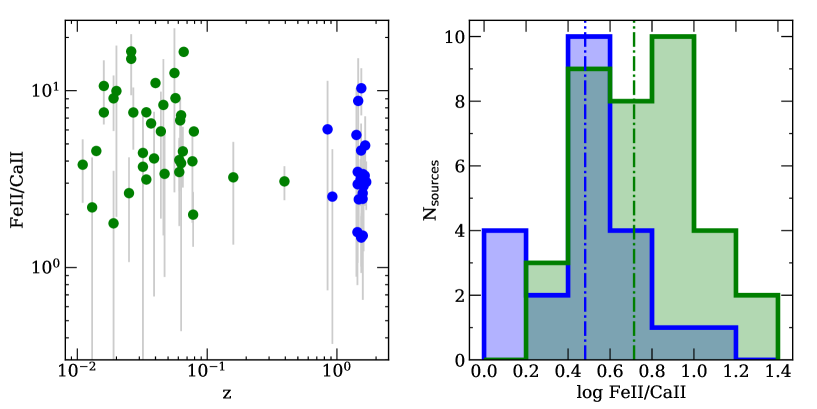
Figure 8: Left panel: Fe ii/CaT distribution as a function of redshift in log-scale. Green symbols correspond to sources with $z<0.8$, the rest of the sources are marked with blue symbols. Right panel: Fe ii/CaT distribution, colors are the same as the left panel. Vertical lines mark the median redshift for the low- and high-redshift subsamples.

7 Conclusions

We performed a detailed analysis of the observational correlations present in our CaT-Fe ii sample together with a bootstrap analysis to asses the statistical reliability of the correlations. Throughout a Principal Component Analysis, we identify the primary driver of our sample. We could not find any redshift dependence above $2\sigma$ confidence level. Since our sample is flux-limited, the presented analysis must be confirmed by larger samples in the future. The presented analysis shows the following:

• The correlation with luminosity, black hole mass and Eddington ratio are stronger for CaT than Fe ii. It suggest that CaT is a better proxy for the Eddington ratio than Fe ii. A potential application of this results could be, for example, the correction of the the Radius-Luminosity relation for effects dependent on the accretion rate. However, the bootstrap analysis provides a probability of $50\%$ to detect a false positive relation. Therefore a more complete a sample is needed to confirm this result.

• The EW_Hβ correlates negatively with luminosity (Baldwin effect), while the EW_CaT shows a positive correlation. It stresses the different nature of both low ionization emission lines. In general, the correlations with Eddington ratio are stronger, more reliable and show the smallest errors according to the bootstrap analysis. This supports the Eddington ratio as the driver of the Baldwin effect.

• We performed a principal component analysis (PCA) to deduce the driver for the R_CaT-R_FeII relation observed in our sample. We confirm that the results of the PCA are dependent on the selection of the sample and the chosen quantities. We consider only the directly observable variables (FWHMs, luminosity and EWs) in the final PCA and later correlate the first four eigenvectors to the derived variables (bolometric luminosity, black hole mass, Eddington ratio, the ratios - R_FeII and R_CaT, and the metallicity indicator, Fe ii/CaT). The dominant eigenvector is primarily driven by the combination of black hole mass and luminosity which in turn is reflected in the strong correlation of the first eigenvector with the Eddington ratio. We also notice a noticeable correlation of the primary eigenvector with the metallicity tracer, Fe ii/CaT.

• Combining the PCA results and the observational correlation, we conclude that luminosity, black hole mass, and Eddington ratio are the main drivers of our sample, however, the correlations are better described by the Eddington ratio, setting this parameter one step ahead in comparison to the other parameters. A larger, more complete sample spanning a larger redshift range including a wide variety of AGN is needed to assert the driver(s) of the CaT-Fe ii correlations.

• We found a significant negative increment of the Fe ii/CaT ratio as a function of redshift, suggesting the effect of a recent starburst which enhanced the $\alpha$-elements with respect to iron at intermediate-redshift. So, the Fe ii/CaT ratio could be used to map the metal and the star formation in AGN. The Fe ii/CaT ratio is also highlighted by the PCA, pointing out the relevance of the metal content in our sample. The negative correlation with the Eddington ratio corroborated by the bootstrap analysis supports the Fe ii/CaT as a metal indicator instead of the typical Fe ii/Mg ii$\lambda 2800$ ratio used for this purpose. However, a more complete sample and sources at large redshift are needed to verify these results.

Appendix A Tables

In this section, we summarize the observational properties of the full sample employed in the analysis. The description of the columns is included in the notes of each table.

Table A.1: Observational parameters

Object

$z$

log $L_{\rm opt}$

log $L_{\rm NIR}$

RFeII

RCaT

FWHM H$\beta$

FWHM OI

FWMH CaII

EW H$\beta$

EW OI

EW CaII

EW FeII

[erg s-1]

[erg s-1]

[ km s-1]

[ km s-1]

[ km s-1]

[Å]

[Å]

[Å]

[Å]

(1)

(2)

(3)

(4)

(5)

(6)

(7)

(8)

(9)

(10)

(11)

(12)

(13)

Persson (1988) Sample

IZw1$\dagger$

0.061

44.684 $\pm$ 0.048

44.694 $\pm$ 0.049

1.78 $\pm$ 0.05

0.51 $\pm$ 0.13

950 $\pm$ 100

600 $\pm$ 150

1150 $\pm$ 150

66 $\pm$ 5

13 $\pm$ 1

43 $\pm$ 4

119 $\pm$ 12

Mrk 42

0.025

43.299 $\pm$ 0.048

43.247 $\pm$ 0.049

1.07 $\pm$ 0.07

0.41 $\pm$ 0.14

500 $\pm$ 100

450 $\pm$ 150

800 $\pm$ 150

36 $\pm$ 2

13 $\pm$ 1

19 $\pm$ 2

40 $\pm$ 6

Mrk 478$\dagger$

0.077

44.685 $\pm$ 0.048

44.607 $\pm$ 0.049

0.93 $\pm$ 0.06

0.23 $\pm$ 0.07

1250 $\pm$ 100

1100 $\pm$ 150

2500 $\pm$ 200

78 $\pm$ 5

18 $\pm$ 2

28 $\pm$ 3

77 $\pm$ 10

II Zw 136

0.063

44.47 $\pm$ 0.048

44.424 $\pm$ 0.049

0.66 $\pm$ 0.05

0.17 $\pm$ 0.13

1850 $\pm$ 100

1200 $\pm$ 150

2300 $\pm$ 250

96 $\pm$ 7

25 $\pm$ 3

29 $\pm$ 6

68 $\pm$ 7

Mrk 231

0.044

44.456 $\pm$ 0.048

44.59 $\pm$ 0.049

2.46 $\pm$ 0.05

0.42 $\pm$ 0.19

5700 $\pm$ 100

3500 $\pm$ 150

1900 $\pm$ 250

50 $\pm$ 4

36 $\pm$ 5

53 $\pm$ 5

120 $\pm$ 10

3C 273

0.159

46.097 $\pm$ 0.048

45.833 $\pm$ 0.049

0.40 $\pm$ 0.05

0.12 $\pm$ 0.04

3800 $\pm$ 100

1900 $\pm$ 150

2250 $\pm$ 250

89 $\pm$ 6

22 $\pm$ 5

27 $\pm$ 5

40 $\pm$ 4

Mrk 6

0.019

43.556 $\pm$ 0.048

43.675 $\pm$ 0.049

0.83 $\pm$ 0.16

0.47 $\pm$ 0.43

2800 $\pm$ 200

1650 $\pm$ 200

1950 $\pm$ 200

29 $\pm$ 6

5 $\pm$ 2

15 $\pm$ 6

24 $\pm$ 7

Mrk 486

0.039

43.969 $\pm$ 0.048

43.892 $\pm$ 0.049

0.27 $\pm$ 0.06

0.07 $\pm$ 0.04

1450 $\pm$ 100

1450 $\pm$ 150

1300 $\pm$ 250

105 $\pm$ 5

23 $\pm$ 3

12 $\pm$ 6

31 $\pm$ 4

Mrk 1239$\dagger$

0.02

43.158 $\pm$ 0.048

44.2 $\pm$ 0.049

1.10 $\pm$ 0.07

0.11 $\pm$ 0.07

750 $\pm$ 100

950 $\pm$ 150

1550 $\pm$ 400

95 $\pm$ 5

25 $\pm$ 3

10 $\pm$ 5

103 $\pm$ 15

Mrk 766

0.013

43.468 $\pm$ 0.048

43.221 $\pm$ 0.049

0.68 $\pm$ 0.12

0.31 $\pm$ 0.25

700 $\pm$ 100

1050 $\pm$ 150

1450 $\pm$ 300

44 $\pm$ 3

12 $\pm$ 2

11 $\pm$ 5

29 $\pm$ 8

Zw 0033+45

0.047

44.352 $\pm$ 0.048

44.159 $\pm$ 0.049

0.53 $\pm$ 0.10

0.16 $\pm$ 0.08

2300 $\pm$ 200

2050 $\pm$ 200

2600 $\pm$ 400

110 $\pm$ 10

23 $\pm$ 4

27 $\pm$ 3

60 $\pm$ 12

Mrk 684

0.046

44.161 $\pm$ 0.048

44.2 $\pm$ 0.049

1.29 $\pm$ 0.07

0.16 $\pm$ 0.10

1300 $\pm$ 100

850 $\pm$ 150

850 $\pm$ 250

38 $\pm$ 4

5 $\pm$ 2

8 $\pm$ 4

51 $\pm$ 7

Mrk 335$\dagger$

0.026

43.974 $\pm$ 0.048

43.932 $\pm$ 0.049

$\leq$0.417

$\leq$0.025

1450 $\pm$ 100

1000 $\pm$ 150

–

86 $\pm$ 5

17 $\pm$ 2

$\leq$5

40 $\pm$ 6

Mrk 376

0.056

44.367 $\pm$ 0.048

44.367 $\pm$ 0.049

0.62 $\pm$ 0.06

0.05 $\pm$ 0.03

5800 $\pm$ 100

4500 $\pm$ 200

–

101 $\pm$ 10

28 $\pm$ 6

10 $\pm$ 5

67 $\pm$ 7

Mrk 493$\dagger$

0.032

43.678 $\pm$ 0.048

43.356 $\pm$ 0.049

0.78 $\pm$ 0.06

0.21 $\pm$ 0.18

450 $\pm$ 100

450 $\pm$ 150

650 $\pm$ 300

41 $\pm$ 3

7 $\pm$ 1

11 $\pm$ 8

33 $\pm$ 4

Mrk 841

0.037

44.124 $\pm$ 0.048

44.045 $\pm$ 0.049

$\leq$0.209

$\leq$0.032

4950 $\pm$ 100

3300 $\pm$ 150

–

107 $\pm$ 6

21 $\pm$ 3

7 $\pm$ 0

25 $\pm$ 6

Ton 1542

0.063

44.207 $\pm$ 0.048

44.404 $\pm$ 0.049

$\leq$0.363

$\leq$0.05

3800 $\pm$ 100

2850 $\pm$ 250

–

114 $\pm$ 11

24 $\pm$ 3

8 $\pm$ 0

43 $\pm$ 4

VII Zw 118

0.079

44.697 $\pm$ 0.048

44.63 $\pm$ 0.049

$\leq$0.447

$\leq$0.076

3700 $\pm$ 100

2600 $\pm$ 300

–

90 $\pm$ 9

14 $\pm$ 2

5 $\pm$ 0

38 $\pm$ 4

Mrk 124

0.057

43.592 $\pm$ 0.048

44.073 $\pm$ 0.049

$\leq$0.708

$\leq$0.078

1050 $\pm$ 100

1050 $\pm$ 250

–

76 $\pm$ 8

20 $\pm$ 4

7 $\pm$ 0

55 $\pm$ 6

Mrk 9

0.04

44.155 $\pm$ 0.048

43.915 $\pm$ 0.049

$\leq$0.398

$\leq$0.036

3450 $\pm$ 100

2500 $\pm$ 250

–

104 $\pm$ 10

21 $\pm$ 2

7 $\pm$ 0

45 $\pm$ 5

NGC 7469

0.016

43.864 $\pm$ 0.048

43.863 $\pm$ 0.049

$\leq$0.339

$\leq$0.045

2700 $\pm$ 200

1750 $\pm$ 250

–

72 $\pm$ 7

11 $\pm$ 2

4 $\pm$ 0

25 $\pm$ 4

Akn 120

0.034

44.188 $\pm$ 0.048

44.62 $\pm$ 0.049

$\leq$0.468

$\leq$0.062

6300 $\pm$ 100

4900 $\pm$ 400

–

89 $\pm$ 5

22 $\pm$ 4

7 $\pm$ 0

42 $\pm$ 4

Mrk 352

0.014

43.037 $\pm$ 0.048

43.136 $\pm$ 0.049

$\leq$0.219

$\leq$0.048

3750 $\pm$ 100

3250 $\pm$ 300

–

83 $\pm$ 5

19 $\pm$ 4

6 $\pm$ 0

19 $\pm$ 4

Mrk 304

0.066

44.507 $\pm$ 0.048

44.416 $\pm$ 0.049

$\leq$0.282

$\leq$0.017

3300 $\pm$ 200

3300 $\pm$ 400

–

118 $\pm$ 6

11 $\pm$ 2

4 $\pm$ 0

36 $\pm$ 6

Mrk 509

0.034

44.508 $\pm$ 0.048

44.43 $\pm$ 0.049

$\leq$0.129

$\leq$0.041

6000 $\pm$ 200

2500 $\pm$ 200

–

125 $\pm$ 6

28 $\pm$ 3

10 $\pm$ 0

18 $\pm$ 3

Martínez-Aldama et al. (2015a, b) Sample

HE 1349+0007

1.444

47.119 $\pm$ 0.047

46.887 $\pm$ 0.045

0.692 $\pm$ 0.143

0.234 $\pm$ 0.086

5027 $\pm$ 430

4580 $\pm$ 680

4530 $\pm$ 940

33.5 $\pm$ 4

19.9 $\pm$ 4

24.7 $\pm$ 7

18.5 $\pm$ 1

HE 1409+0101

1.65

47.629 $\pm$ 0.044

47.264 $\pm$ 0.048

1.549 $\pm$ 0.107

0.316 $\pm$ 0.066

4000 $\pm$ 160

3100 $\pm$ 310

3550 $\pm$ 500

26.8 $\pm$ 1

15.3 $\pm$ 2

19.9 $\pm$ 6

36.2 $\pm$ 2

HE 2349-3800

1.604

47.11 $\pm$ 0.044

46.933 $\pm$ 0.045

0.832 $\pm$ 0.057

0.288 $\pm$ 0.093

4000 $\pm$ 160

3480 $\pm$ 520

3520 $\pm$ 700

27.1 $\pm$ 1

17.6 $\pm$ 4

19.9 $\pm$ 6

19.9 $\pm$ 1

HE 2147-3212

1.543

47.163 $\pm$ 0.049

46.891 $\pm$ 0.045

1.479 $\pm$ 0.375

0.49 $\pm$ 0.079

4491 $\pm$ 660

4300 $\pm$ 860

3990 $\pm$ 150

28.4 $\pm$ 3

22.1 $\pm$ 6

47.4 $\pm$ 4

35 $\pm$ 4

HE 2202-2557

1.535

47.172 $\pm$ 0.048

46.585 $\pm$ 0.043

0.537 $\pm$ 0.062

0.117 $\pm$ 0.019

7000 $\pm$ 540

5810 $\pm$ 1060

5900 $\pm$ 330

27.4 $\pm$ 1

3.6 $\pm$ 1

13 $\pm$ 3

12.7 $\pm$ 1

HE 2340-4443

0.922

46.758 $\pm$ 0.046

46.674 $\pm$ 0.049

0.224 $\pm$ 0.021

0.089 $\pm$ 0.064

3200 $\pm$ 100

3430 $\pm$ 220

3190 $\pm$ 1700

77.5 $\pm$ 3

15.9 $\pm$ 1

14.8 $\pm$ 10

15.4 $\pm$ 1

HE 0248-3628

1.536

47.465 $\pm$ 0.045

47.222 $\pm$ 0.044

0.372 $\pm$ 0.034

0.251 $\pm$ 0.023

3800 $\pm$ 150

3490 $\pm$ 260

3990 $\pm$ 150

40.7 $\pm$ 2

12.2 $\pm$ 2

31.3 $\pm$ 2

13.6 $\pm$ 0.5

HE 2352-4010

1.58

47.727 $\pm$ 0.044

47.537 $\pm$ 0.05

0.447 $\pm$ 0.031

0.17 $\pm$ 0.023

2900 $\pm$ 90

1930 $\pm$ 110

3080 $\pm$ 180

45.3 $\pm$ 1

16.6 $\pm$ 2

21.7 $\pm$ 3

17.6 $\pm$ 0.3

HE 0035-2853

1.638

47.309 $\pm$ 0.048

47.177 $\pm$ 0.044

1.479 $\pm$ 0.17

0.447 $\pm$ 0.041

5141 $\pm$ 390

5000 $\pm$ 370

4540 $\pm$ 170

30.3 $\pm$ 1

9.4 $\pm$ 2

27.9 $\pm$ 2

40.7 $\pm$ 3

HE 0048-2804

0.847

46.032 $\pm$ 0.049

46.168 $\pm$ 0.044

0.617 $\pm$ 0.114

0.102 $\pm$ 0.075

5484 $\pm$ 470

4990 $\pm$ 270

5170 $\pm$ 2400

40.1 $\pm$ 4

18.4 $\pm$ 1

4.9 $\pm$ 3

22.3 $\pm$ 2

HE 0058-3231

1.582

47.336 $\pm$ 0.048

47.043 $\pm$ 0.055

0.589 $\pm$ 0.176

0.389 $\pm$ 0.09

5127 $\pm$ 160

4960 $\pm$ 100

4910 $\pm$ 760

55.4 $\pm$ 2

44.4 $\pm$ 8

59.6 $\pm$ 14

27.7 $\pm$ 2

HE 0203-4627

1.438

47.102 $\pm$ 0.048

46.941 $\pm$ 0.045

0.759 $\pm$ 0.192

0.479 $\pm$ 0.088

5486 $\pm$ 810

6000 $\pm$ 250

5960 $\pm$ 530

26.1 $\pm$ 3

13.6 $\pm$ 3

33.2 $\pm$ 3

14.4 $\pm$ 2

HE 0005-2355

1.412

47.161 $\pm$ 0.047

46.863 $\pm$ 0.045

0.933 $\pm$ 0.237

0.166 $\pm$ 0.107

4777 $\pm$ 710

3500 $\pm$ 820

4600 $\pm$ 1070

21.8 $\pm$ 2

7.8 $\pm$ 2

13.9 $\pm$ 8

17.2 $\pm$ 2

HE 0043-2300

1.54

47.409 $\pm$ 0.05

47.257 $\pm$ 0.045

0.316 $\pm$ 0.044

0.214 $\pm$ 0.025

3511 $\pm$ 110

4000 $\pm$ 360

4000 $\pm$ 150

69.3 $\pm$ 5

24.5 $\pm$ 3

36.1 $\pm$ 3

20 $\pm$ 1

HE 0349-5249

1.541

47.567 $\pm$ 0.047

46.826 $\pm$ 0.049

1.704 $\pm$ 0.102

0.165 $\pm$ 0.014

4000 $\pm$ 400

3810 $\pm$ 220

4000 $\pm$ 150

21.9 $\pm$ 2.4

13.5 $\pm$ 3

37.6 $\pm$ 8

32.1 $\pm$ 3.5

HE 0359-3959

1.521

47.132 $\pm$ 0.047

46.911 $\pm$ 0.049

1.173 $\pm$ 0.07

0.371 $\pm$ 0.031

4000 $\pm$ 400

1770 $\pm$ 320

1560 $\pm$ 60

40.6 $\pm$ 4.4

9.2 $\pm$ 2.1

46.6 $\pm$ 9.9

43.3 $\pm$ 4.7

HE 0436-3709

1.445

46.949 $\pm$ 0.062

46.855 $\pm$ 0.046

1.164 $\pm$ 0.07

0.335 $\pm$ 0.028

4491 $\pm$ 449

4440 $\pm$ 250

4610 $\pm$ 170

33.8 $\pm$ 3.7

13.9 $\pm$ 1.9

26.8 $\pm$ 5.7

33.7 $\pm$ 3.7

HE 0507-3236

1.577

47.094 $\pm$ 0.044

46.939 $\pm$ 0.063

0.291 $\pm$ 0.006

0.119 $\pm$ 0.034

3200 $\pm$ 320

2830 $\pm$ 420

3870 $\pm$ 800

71.3 $\pm$ 7.2

25.1 $\pm$ 6.1

23.4 $\pm$ 8.2

17.8 $\pm$ 1.8

HE 0512-3329

1.587

47.222 $\pm$ 0.044

47.095 $\pm$ 0.064

0.81 $\pm$ 0.017

0.24 $\pm$ 0.05

3800 $\pm$ 380

2170 $\pm$ 320

2320 $\pm$ 360

75.6 $\pm$ 7.6

26.7 $\pm$ 6.5

46.6 $\pm$ 13.4

53.5 $\pm$ 5.4

HE 0926-0201

1.682

47.572 $\pm$ 0.049

47.338 $\pm$ 0.054

1.139 $\pm$ 0.082

0.374 $\pm$ 0.033

2900 $\pm$ 290

4310 $\pm$ 380

4500 $\pm$ 170

27.6 $\pm$ 3.1

28.9 $\pm$ 4.3

33.1 $\pm$ 7

27.6 $\pm$ 3.1

HE 1039-0724

1.458

47.027 $\pm$ 0.049

46.882 $\pm$ 0.05

0.289 $\pm$ 0.021

0.033 $\pm$ 0.018

5141 $\pm$ 514

3810 $\pm$ 890

3970 $\pm$ 920

28.4 $\pm$ 3.2

11.5 $\pm$ 3.4

2.7 $\pm$ 1.6

6.7 $\pm$ 0.8

HE 1120+0154

1.472

47.568 $\pm$ 0.047

47.363 $\pm$ 0.052

0.204 $\pm$ 0.012

0.084 $\pm$ 0.011

5498 $\pm$ 550

4030 $\pm$ 230

4040 $\pm$ 220

31 $\pm$ 3.4

13.3 $\pm$ 1.9

8.1 $\pm$ 1.9

5.4 $\pm$ 0.6

Marinello et al. (2016) Sample

1H 1934-063$\dagger$

0.011

42.624 $\pm$ 0.043

42.637 $\pm$ 0.044

1.404 $\pm$ 0.223

0.368 $\pm$ 0.047

1430 $\pm$ 100

1000 $\pm$ 80

1205 $\pm$ 84

35.3 $\pm$ 3.5

18.8 $\pm$ 1.3

29.4 $\pm$ 1.9

53.2 $\pm$ 5.1

1H 2107-097$\dagger$

0.027

43.217 $\pm$ 0.043

43.465 $\pm$ 0.044

1.047 $\pm$ 0.106

0.139 $\pm$ 0.019

2530 $\pm$ 320

1720 $\pm$ 138

1700 $\pm$ 136

38 $\pm$ 3.4

14.4 $\pm$ 1.5

14.2 $\pm$ 1.5

34.9 $\pm$ 3.6

IZw1$\dagger$

0.061

44.344 $\pm$ 0.043

44.195 $\pm$ 0.044

2.286 $\pm$ 0.199

0.564 $\pm$ 0.058

1450 $\pm$ 110

820 $\pm$ 57

1100 $\pm$ 77

38.1 $\pm$ 2.9

33.9 $\pm$ 1.8

73.4 $\pm$ 4.1

84.9 $\pm$ 4.9

Mrk 1044$\dagger$

0.016

43.076 $\pm$ 0.043

43.013 $\pm$ 0.046

1.181 $\pm$ 0.127

0.111 $\pm$ 0.016

1570 $\pm$ 145

1010 $\pm$ 61

1200 $\pm$ 72

57.2 $\pm$ 5.1

18.9 $\pm$ 1.2

24.6 $\pm$ 2.1

65.3 $\pm$ 5.7

Mrk 1239$\dagger$

0.019

43.19 $\pm$ 0.043

43.366 $\pm$ 0.051

1.34 $\pm$ 0.147

0.148 $\pm$ 0.016

1720 $\pm$ 130

1220 $\pm$ 98

1240 $\pm$ 74

64.3 $\pm$ 5.3

23.3 $\pm$ 1.9

20.1 $\pm$ 2.2

74.8 $\pm$ 6.2

Mrk 335$\dagger$

0.026

43.82 $\pm$ 0.043

43.721 $\pm$ 0.053

0.818 $\pm$ 0.092

0.054 $\pm$ 0.007

1715 $\pm$ 130

1140 $\pm$ 103

1490 $\pm$ 119

123.8 $\pm$ 7.6

25.2 $\pm$ 1.7

11.3 $\pm$ 1.1

100.5 $\pm$ 8.8

Mrk 478$\dagger$

0.078

44.258 $\pm$ 0.043

44.45 $\pm$ 0.044

1.023 $\pm$ 0.089

0.514 $\pm$ 0.056

1250 $\pm$ 100

1300 $\pm$ 91

1560 $\pm$ 94

76.9 $\pm$ 6.1

20.8 $\pm$ 1.7

19.9 $\pm$ 1.6

55.2 $\pm$ 4.9

Mrk 493$\dagger$

0.032

43.393 $\pm$ 0.043

43.515 $\pm$ 0.044

1.721 $\pm$ 0.179

0.387 $\pm$ 0.046

1450 $\pm$ 110

770 $\pm$ 31

1065 $\pm$ 64

62.5 $\pm$ 5.9

13.3 $\pm$ 1.1

17.5 $\pm$ 1.4

33.3 $\pm$ 1.8

PG 1448+273$\dagger$

0.065

44.305 $\pm$ 0.043

44.064 $\pm$ 0.044

1.189 $\pm$ 0.129

0.262 $\pm$ 0.034

1730 $\pm$ 135

880 $\pm$ 35

885 $\pm$ 44

31.2 $\pm$ 3.8

15.2 $\pm$ 1

18.8 $\pm$ 1.3

32.2 $\pm$ 1.8

Tons 180$\dagger$

0.062

44.283 $\pm$ 0.043

43.911 $\pm$ 0.058

0.985 $\pm$ 0.11

0.145 $\pm$ 0.015

1470 $\pm$ 135

930 $\pm$ 41

990 $\pm$ 59

32.3 $\pm$ 1.9

9.6 $\pm$ 0.7

19.5 $\pm$ 1.6

31.1 $\pm$ 2.2

Marinello et al. (2020) Sample

PHL 1092

0.394

44.883 $\pm$ 0.043

44.604 $\pm$ 0.047

2.576 $\pm$ 0.108

0.839 $\pm$ 0.038

1850 $\pm$ 100

1250 $\pm$ 100

3750 $\pm$ 360

34.2 $\pm$ 2.2

24.4 $\pm$ 1.8

90.2 $\pm$ 7.1

88.5 $\pm$ 5.3

Notes. Columns are as follows: (1) Object name. (2) Redshift. (3) Optical continuum luminosity at 5100Å. (4) NIR luminosity at 8542Å. (5) and (6) R_FeII and CaT values, respectively. (7), (8) and (9) Full-width at half maximum of H$\beta$, O i $\lambda 8446$ and CaT in units of  km s^-1, respectively. (10), (11), (12) and (13) Equivalent width of H$\beta$, O i $\lambda 8446$, CaT and Fe ii  in units of Å, respectively.

Table A.2: Black hole parameters

Object	log $M\mathrm{{}_{BH}}$	log $L\mathrm{{}_{bol}}/L\mathrm{{}_{Edd}}$
	[$M_{\odot}$]
(1)	(2)	(4)
Persson (1988) Sample
IZw1$\dagger$	7.935 ${}^{+0.177}_{-0.177}$	-0.362 ${}^{+0.184}_{-0.184}$
Mrk 42	6.966 ${}^{+0.257}_{-0.257}$	-0.501 ${}^{+0.262}_{-0.262}$
Mrk 478$\dagger$	8.035 ${}^{+0.158}_{-0.158}$	-0.461 ${}^{+0.165}_{-0.165}$
II Zw 136	8.061 ${}^{+0.138}_{-0.138}$	-0.66 ${}^{+0.147}_{-0.147}$
Mrk 231	8.46 ${}^{+0.121}_{-0.121}$	-1.069 ${}^{+0.131}_{-0.131}$
3C 273	9.188 ${}^{+0.142}_{-0.14}$	-0.485 ${}^{+0.15}_{-0.148}$
Mrk 6	7.724 ${}^{+0.141}_{-0.141}$	-1.053 ${}^{+0.149}_{-0.149}$
Mrk 486	7.707 ${}^{+0.148}_{-0.148}$	-0.705 ${}^{+0.156}_{-0.156}$
Mrk 1239$\dagger$	7.037 ${}^{+0.201}_{-0.201}$	-0.684 ${}^{+0.207}_{-0.206}$
Mrk 766	7.177 ${}^{+0.207}_{-0.207}$	-0.577 ${}^{+0.213}_{-0.213}$
Zw 0033+45	8.077 ${}^{+0.151}_{-0.151}$	-0.769 ${}^{+0.159}_{-0.159}$
Mrk 684	7.77 ${}^{+0.154}_{-0.154}$	-0.615 ${}^{+0.161}_{-0.161}$
Mrk 335$\dagger$	7.709 ${}^{+0.148}_{-0.148}$	-0.704 ${}^{+0.156}_{-0.156}$
Mrk 376	8.419 ${}^{+0.121}_{-0.121}$	-1.099 ${}^{+0.131}_{-0.131}$
Mrk 493$\dagger$	7.129 ${}^{+0.276}_{-0.276}$	-0.361 ${}^{+0.28}_{-0.28}$
Mrk 841	8.232 ${}^{+0.12}_{-0.12}$	-1.107 ${}^{+0.13}_{-0.13}$
Ton 1542	8.181 ${}^{+0.122}_{-0.122}$	-0.989 ${}^{+0.131}_{-0.131}$
VII Zw 118	8.432 ${}^{+0.124}_{-0.124}$	-0.849 ${}^{+0.134}_{-0.134}$
Mrk 124	7.389 ${}^{+0.168}_{-0.168}$	-0.69 ${}^{+0.175}_{-0.175}$
Mrk 9	8.118 ${}^{+0.123}_{-0.123}$	-0.968 ${}^{+0.132}_{-0.132}$
NGC 7469	7.875 ${}^{+0.142}_{-0.142}$	-0.957 ${}^{+0.15}_{-0.15}$
Akn 120	8.353 ${}^{+0.121}_{-0.121}$	-1.177 ${}^{+0.13}_{-0.13}$
Mrk 352	7.553 ${}^{+0.126}_{-0.126}$	-1.297 ${}^{+0.136}_{-0.135}$
Mrk 304	8.289 ${}^{+0.135}_{-0.135}$	-0.858 ${}^{+0.144}_{-0.144}$
Mrk 509	8.506 ${}^{+0.125}_{-0.125}$	-1.074 ${}^{+0.134}_{-0.134}$
Martínez-Aldama et al. (2015a, b) Sample
HE 1349+0007	9.834 ${}^{+0.183}_{-0.179}$	-0.313 ${}^{+0.189}_{-0.185}$
HE 1409+0101	10.023 ${}^{+0.178}_{-0.173}$	-0.094 ${}^{+0.184}_{-0.179}$
HE 2349-3800	9.746 ${}^{+0.166}_{-0.162}$	-0.233 ${}^{+0.172}_{-0.168}$
HE 2147-3212	9.817 ${}^{+0.219}_{-0.216}$	-0.260 ${}^{+0.225}_{-0.222}$
HE 2202-2557	9.981 ${}^{+0.181}_{-0.177}$	-0.418 ${}^{+0.188}_{-0.184}$
HE 2340-4443	9.479 ${}^{+0.157}_{-0.154}$	-0.246 ${}^{+0.164}_{-0.160}$
HE 0248-3628	9.917 ${}^{+0.174}_{-0.169}$	-0.119 ${}^{+0.180}_{-0.175}$
HE 2352-4010	9.960 ${}^{+0.180}_{-0.175}$	0.048 ${}^{+0.185}_{-0.180}$
HE 0035-2853	9.943 ${}^{+0.183}_{-0.178}$	-0.270 ${}^{+0.189}_{-0.185}$
HE 0048-2804	9.286 ${}^{+0.163}_{-0.161}$	-0.634 ${}^{+0.171}_{-0.169}$
HE 0058-3231	9.956 ${}^{+0.169}_{-0.165}$	-0.262 ${}^{+0.176}_{-0.172}$
HE 0203-4627	9.856 ${}^{+0.219}_{-0.216}$	-0.348 ${}^{+0.224}_{-0.222}$
HE 0005-2355	9.838 ${}^{+0.220}_{-0.217}$	-0.283 ${}^{+0.226}_{-0.223}$
HE 0043-2300	9.859 ${}^{+0.172}_{-0.167}$	-0.106 ${}^{+0.179}_{-0.175}$
HE 0349-5249	9.990 ${}^{+0.199}_{-0.195}$	-0.110 ${}^{+0.205}_{-0.201}$
HE 0359-3959	9.758 ${}^{+0.190}_{-0.187}$	-0.227 ${}^{+0.196}_{-0.193}$
HE 0436-3709	9.703 ${}^{+0.188}_{-0.185}$	-0.317 ${}^{+0.198}_{-0.195}$
HE 0507-3236	9.658 ${}^{+0.190}_{-0.186}$	-0.156 ${}^{+0.195}_{-0.192}$
HE 0512-3329	9.788 ${}^{+0.192}_{-0.188}$	-0.184 ${}^{+0.197}_{-0.193}$
HE 0926-0201	9.877 ${}^{+0.201}_{-0.196}$	0.007 ${}^{+0.207}_{-0.203}$
HE 1039-0724	9.793 ${}^{+0.188}_{-0.185}$	-0.345 ${}^{+0.195}_{-0.191}$
HE 1120+0154	10.105 ${}^{+0.200}_{-0.195}$	-0.225 ${}^{+0.205}_{-0.201}$
Marinello et al. (2016) Sample
1H 1934-063$\dagger$	6.985 ${}^{+0.156}_{-0.155}$	-1.059 ${}^{+0.162}_{-0.161}$
1H 2107-097$\dagger$	7.507 ${}^{+0.178}_{-0.178}$	-1.107 ${}^{+0.183}_{-0.183}$
IZw1$\dagger$	7.907 ${}^{+0.151}_{-0.151}$	-0.605 ${}^{+0.158}_{-0.158}$
Mrk 1044$\dagger$	7.259 ${}^{+0.162}_{-0.162}$	-0.973 ${}^{+0.168}_{-0.167}$
Mrk 1239$\dagger$	7.353 ${}^{+0.151}_{-0.15}$	-0.975 ${}^{+0.157}_{-0.157}$
Mrk 335$\dagger$	7.688 ${}^{+0.148}_{-0.148}$	-0.805 ${}^{+0.155}_{-0.155}$
Mrk 478$\dagger$	7.807 ${}^{+0.156}_{-0.156}$	-0.575 ${}^{+0.162}_{-0.162}$
Mrk 493$\dagger$	7.399 ${}^{+0.152}_{-0.152}$	-0.859 ${}^{+0.158}_{-0.158}$
PG 1448+273$\dagger$	7.949 ${}^{+0.15}_{-0.149}$	-0.679 ${}^{+0.156}_{-0.156}$
Tons 180$\dagger$	7.879 ${}^{+0.16}_{-0.16}$	-0.626 ${}^{+0.166}_{-0.166}$
Marinello et al. (2020) Sample
PHL 1092	8.281 ${}^{+0.140}_{-0.140}$	-0.549 ${}^{+0.147}_{-0.147}$

NOTES. Columns are as follows: (1) Object name. (2) Black hole mass estimated using the classical RL relation (Eq. 3), in units of M_⊙ . (3) Eddington ratio.

Table A.3: Parameters of the correlations for the observed and bootstrap sample

		Observational data						Bootstrap results
Relation		$\alpha$	$\beta$	$\rho$	$p$-value	$\sigma$		$\alpha_{\rm BS}$	$\beta_{\rm BS}$	${\rho_{\rm BS}}$	$f_{sig}$	P. Dist.	$p-$valueran	$f_{\rm ran}$
(1)		(2)	(3)	(4)	(5)	(6)		(7)	(8)	(9)	(10)	(11)	(12)	(13)
EWHβ	$L_{\mathrm{opt}}$	-0.064 $\pm$ 0.032	4.632 $\pm$ 1.469	-0.412	0.001	0.200		-0.064 $\pm$ 0.031	4.618 $\pm$ 1.408	-0.428${}^{+0.21}_{-0.17}$	0.5	c,a,b	0.76,0.95, 0.67	3.5$\times 10^{-3}$
	$L_{\rm NIR}$	-0.064 $\pm$ 0.036	4.627 $\pm$ 1.618	-0.352	0.007	0.204		-0.065 $\pm$ 0.034	4.656 $\pm$ 1.430	-0.372${}^{+0.22}_{-0.17}$	0.2	c,c,d	0.76,0.98,0.60	1.0$\times 10^{-3}$
	$M\mathrm{{}_{BH}}$	-0.091 $\pm$ 0.053	2.508 $\pm$ 0.455	-0.390	0.002	0.206		-0.092 $\pm$ 0.048	2.519 $\pm$ 0.409	-0.405${}^{+0.24}_{-0.19}$	0.4	c,b,d	0.76,0.96,0.94	1.0$\times 10^{-3}$
	$L\mathrm{{}_{bol}}/L\mathrm{{}_{Edd}}$	-0.332 $\pm$ 0.149	1.53 $\pm$ 0.102	-0.531	1.78$\times 10^{-5}$	0.195		-0.335 $\pm$ 0.148	1.529 $\pm$ 0.09	-0.544${}^{+0.19}_{-0.16}$	0.85	c,c	0.76,0.61	1.5$\times 10^{-3}$
EWOI	$L_{\mathrm{opt}}$	-0.007 $\pm$ 0.034	1.557 $\pm$ 1.548	-0.015	0.910	0.211		-0.007 $\pm$ 0.033	1.000 $\pm$ 1.510	-0.016${}^{+0.23}_{-0.27}$	0.0	e,a,b	0.97,0.95,0.67	1.0$\times 10^{-3}$
	$L_{\rm NIR}$	-0.003 $\pm$ 0.037	1.358 $\pm$ 1.673	0.053	0.691	0.211		-0.003 $\pm$ 0.034	1.358 $\pm$ 1.603	0.060${}^{+0.20}_{-0.28}$	0.0	e,c,d	0.97,0.98,0.60	1.5$\times 10^{-3}$
	$M\mathrm{{}_{BH}}$	-0.006 $\pm$ 0.054	1.271 $\pm$ 0.468	-0.008	0.951	0.211		-0.005 $\pm$ 0.057	1.264 $\pm$ 0.459	0.008${}^{+0.23}_{-0.27}$	0.0	e,b,d	0.97,0.96,0.94	1.0$\times 10^{-3}$
	$L\mathrm{{}_{bol}}/L\mathrm{{}_{Edd}}$	-0.079 $\pm$ 0.161	1.172 $\pm$ 0.110	-0.162	0.223	0.209		-0.082 $\pm$ 0.142	1.169 $\pm$ 0.107	-0.161${}^{+0.23}_{-0.26}$	0.0	e,c	0.97,0.61	5.0$\times 10^{-4}$
EWFeII	$L_{\mathrm{opt}}$	-0.091 $\pm$ 0.039	5.666 $\pm$ 1.754	-0.409	0.001	0.239		-0.092 $\pm$ 0.039	5.678 $\pm$ 1.705	-0.422${}^{+0.22}_{-0.17}$	0.5	a,a,b	0.94,0.95,0.67	5.0$\times 10^{-4}$
	$L_{\rm NIR}$	-0.095 $\pm$ 0.042	5.846 $\pm$ 1.917	-0.367	0.005	0.242		-0.096 $\pm$ 0.043	5.881 $\pm$ 1.809	-0.385${}^{+0.23}_{-0.18}$	0.3	a,c,d	0.94,0.95,0.55	5.0$\times 10^{-4}$
	$M\mathrm{{}_{BH}}$	-0.151 $\pm$ 0.06	2.831 $\pm$ 0.52	-0.493	8.58$\times 10^{-5}$	0.234		-0.15 $\pm$ 0.059	2.824 $\pm$ 0.52	-0.517${}^{+0.21}_{-0.14}$	0.75	a,b,d	0.94,0.96,0.94	1.0$\times 10^{-3}$
	$L\mathrm{{}_{bol}}/L\mathrm{{}_{Edd}}$	-0.281 $\pm$ 0.203	1.373 $\pm$ 0.139	-0.360	0.005	0.265		-0.279 $\pm$ 0.211	1.374 $\pm$ 0.142	-0.375${}^{+0.22}_{-0.19}$	0.3	a,c	0.94,0.61	5.0$\times 10^{-4}$
EWCaT	$L_{\mathrm{opt}}$	0.068 $\pm$ 0.053	-1.851 $\pm$ 2.381	0.417	0.001	0.324		0.069 $\pm$ 0.049	-1.896 $\pm$ 1.842	0.425${}^{+0.14}_{-0.25}$	0.5	a,a,b	0.93,0.95,0.67	1.0$\times 10^{-3}$
	$L_{\rm NIR}$	0.068 $\pm$ 0.057	-1.827 $\pm$ 2.593	0.377	0.004	0.327		0.069 $\pm$ 0.051	-1.878 $\pm$ 2.451	0.380${}^{+0.15}_{-0.24}$	0.3	a,c,d	0.93,0.98, 0.60	1.5$\times 10^{-3}$
	$M\mathrm{{}_{BH}}$	0.088 $\pm$ 0.085	0.470 $\pm$ 0.733	0.301	0.022	0.331		0.089 $\pm$ 0.074	0.456 $\pm$ 0.608	0.305${}^{+0.17}_{-0.23}$	0.1	a,b,d	0.93,0.96,0.94	1.0$\times 10^{-3}$
	$L\mathrm{{}_{bol}}/L\mathrm{{}_{Edd}}$	0.428 $\pm$ 0.237	1.477 $\pm$ 0.162	0.482	1.27$\times 10^{-4}$	0.309		0.431 $\pm$ 0.200	1.477 $\pm$ 0.133	0.494${}^{+0.14}_{-0.24}$	0.71	a,c	0.93,0.61	1.0$\times 10^{-3}$
RFeII	$L_{\mathrm{opt}}$	-0.015 $\pm$ 0.049	0.520 $\pm$ 2.209	-0.063	0.640	0.301		-0.015 $\pm$ 0.045	0.536 $\pm$ 1.901	-0.064${}^{+0.22}_{-0.28}$	0.0	e,a,b	0.96,0.95,0.67	1.5$\times 10^{-3}$
	$L_{\rm NIR}$	-0.017 $\pm$ 0.053	0.631 $\pm$ 2.383	-0.081	0.546	0.301		-0.017 $\pm$ 0.047	0.602 $\pm$ 2.264	-0.083${}^{+0.22}_{-0.26}$	0.0	e,c,d	0.96,0.98,0.60	5.0$\times 10^{-4}$
	$M\mathrm{{}_{BH}}$	-0.042 $\pm$ 0.076	0.204 $\pm$ 0.662	-0.162	0.226	0.299		-0.042 $\pm$ 0.065	0.205 $\pm$ 0.566	-0.160${}^{+0.22}_{-0.25}$	0.0	e,b,d	0.96,0.96,0.94	2.0$\times 10^{-3}$
	$L\mathrm{{}_{bol}}/L\mathrm{{}_{Edd}}$	0.109 $\pm$ 0.230	-0.092 $\pm$ 0.157	0.105	0.432	0.300		0.111 $\pm$ 0.239	-0.088 $\pm$ 0.141	0.102${}^{+0.25}_{-0.29}$	0.0	e,c	0.96,0.61	1.0$\times 10^{-3}$
RCaT	$L_{\mathrm{opt}}$	0.057 $\pm$ 0.063	-3.392 $\pm$ 2.846	0.247	0.061	0.388		0.056 $\pm$ 0.056	-3.350 $\pm$ 2.437	0.243${}^{+0.18}_{-0.23}$	0.1	f,a,b	0.76,0.95,0.67	3.5$\times 10^{-3}$
	$L_{\rm NIR}$	0.059 $\pm$ 0.068	-3.476 $\pm$ 3.079	0.240	0.069	0.389		0.060 $\pm$ 0.058	-3.502 $\pm$ 2.823	0.241${}^{+0.18}_{-0.24}$	0.1	f,c,d	0.76,0.98,0.60	1.5$\times 10^{-3}$
	$M\mathrm{{}_{BH}}$	0.058 $\pm$ 0.101	-1.309 $\pm$ 0.874	0.117	0.381	0.394		0.058 $\pm$ 0.091	-1.306 $\pm$ 0.762	0.111${}^{+0.20}_{-0.24}$	0.0	f,b,d	0.76,0.96,0.94	1.5$\times 10^{-3}$
	$L\mathrm{{}_{bol}}/L\mathrm{{}_{Edd}}$	0.500 $\pm$ 0.275	-0.516 $\pm$ 0.188	0.425	8.90$\times 10^{-4}$	0.359		0.498 $\pm$ 0.254	-0.516 $\pm$ 0.152	0.426${}^{+0.18}_{-0.25}$	0.51	f,c	0.76,0.61	5.0$\times 10^{-4}$
Fe ii/CaT	$L_{\mathrm{opt}}$	-0.072 $\pm$ 0.039	3.912 $\pm$ 1.78	-0.441	5.31$\times 10^{-4}$	0.242		-0.071 $\pm$ 0.039	3.877 $\pm$ 1.747	-0.444${}^{+0.22}_{-0.22}$	0.54	e,a,b	0.98,0.95,0.67	5.0$\times 10^{-4}$
	$L_{\rm NIR}$	-0.077 $\pm$ 0.043	4.107 $\pm$ 1.929	-0.456	3.20$\times 10^{-4}$	0.244		-0.076 $\pm$ 0.042	4.086 $\pm$ 1.887	-0.470${}^{+0.23}_{-0.20}$	0.61	e,c,d	0.98,0.98,0.60	5.0$\times 10^{-4}$
	$M\mathrm{{}_{BH}}$	-0.100 $\pm$ 0.064	1.513 $\pm$ 0.552	-0.354	0.006	0.249		-0.102 $\pm$ 0.061	1.532 $\pm$ 0.559	-0.348${}^{+0.23}_{-0.24}$	0.3	e,b,d	0.98,0.96,0.94	1.5$\times 10^{-3}$
	$L\mathrm{{}_{bol}}/L\mathrm{{}_{Edd}}$	-0.391 $\pm$ 0.179	0.424 $\pm$ 0.122	-0.554	6.44$\times 10^{-6}$	0.233		-0.394 $\pm$ 0.164	0.422 $\pm$ 0.099	-0.560${}^{+0.20}_{-0.17}$	0.89	e,c	0.98,0.61	1.0$\times 10^{-3}$
RFeII	RCaT	0.973 $\pm$ 0.239	-0.657 $\pm$ 0.081	0.721	1.75$\times 10^{-10}$	0.270		0.974 $\pm$ 0.189	-0.658 $\pm$ 0.07	0.737${}^{+0.07}_{-0.19}$	1.0	e,f	0.96,0.76	2.0$\times 10^{-3}$

NOTES. Columns are as follow: (1) Relations. (2) Slope of the observational sample and error at $2\sigma$. (3) Ordinate of the observational sample and error at $2\sigma$. (4) Spearman rank correlation coefficient for the observational sample. Significant correlations respect to this parameter are bold–faced. (5) $p-$value of the correlation coefficient. (6) Scatter of the observational sample respect to the best fit. (7) Slope of the bootstrap sample and error at $2\sigma$. (8) Ordinate of the bootstrap sample and error at $2\sigma$. (9) Maximum of Spearman rank correlation coefficient distribution for 1000 realizations of the bootstrap sample and the errors at $2\sigma$. (10) Fraction of significant bootstrap realizations respect to the total number. (11) Probability distributions used to model the observational distributions using a random sample. The symbols are as follow: a–skewnorm, b–powernorm, c–powerlaw, d–loglaplace, e–powerlognorm, f–lognorm. The symbols follow the order of col. (1). In correlations involving luminosity and black hole mass, 2 distributions where used in the modelling. (12) $p-$value of the Kolmogorov-Smirnoff test to select the best distribution fitting. Order is the same as col. (11). (13) Fraction of significant correlations assuming a two random samples.

Table A.4: Correlations between the first four eigenvectors and the physical parameters

Relations		Full		Low–$L$		High–$L$
		$\rho$	$p$–value	$\rho$	$p$–value	$\rho$	$p$–value
(1)		(2)	(3)	(4)	(5)	(6)	(7)
PC1	FWHMHβ	-0.792	1.32$\times 10^{-13}$	0.669	7.37$\times 10^{-5}$	0.76	1.73$\times 10^{6}$
	FWHMOI	-0.845	7.51$\times 10^{-17}$	0.728	7.65$\times 10^{-6}$	0.884	2.1$\times 10^{-10}$
	FWHMCaT	-0.844	1.77$\times 10^{-13}$	0.659	0.00159	0.85	3.94$\times 10^{-8}$
	EWHβ	0.583	1.59$\times 10^{-6}$	0.736	5.46$\times 10^{-6}$	-0.694	2.93$\times 10^{-5}$
	EWOI	0.180	0.177	0.871	8.11$\times 10^{-10}$	-0.296	0.12
	EWFeII	0.703	7.79$\times 10^{-10}$	0.476	0.00897	-0.681	4.73$\times 10^{-5}$
	EWCaT	-0.179	0.178	-0.072	0.712	-0.257	0.178
	$z$	-0.700	1$\times 10^{-9}$	0.356	0.0578	0.366	0.0512
	log $L\mathrm{{}_{bol}}$	-0.748	1.49$\times 10^{-11}$	0.495	0.00638	0.458	0.0124
	log $M\mathrm{{}_{BH}}$	-0.845	6.99$\times 10^{-17}$	0.701	2.24$\times 10^{-5}$	0.662	9.16$\times 10^{-5}$
	log $L\mathrm{{}_{bol}}/L\mathrm{{}_{Edd}}$	-0.519	2.94$\times 10^{-5}$	-0.492	0.00672	0.174	0.367
	log RFeII	0.164	0.218	-0.316	0.0952	-0.089	0.645
	log RCaT	-0.151	0.259	-0.382	0.041	-0.021	0.914
	log Fe ii/CaT	0.426	8.46$\times 10^{-4}$	0.338	0.073	-0.125	0.518
PC2	FWHMHβ	0.023	0.864	-0.344	0.0674	-0.278	0.145
	FWHMOI	-0.033	0.804	-0.38	0.0422	0.057	0.769
	FWHMCaT	-0.098	0.518	0.456	0.0435	-0.016	0.939
	EWHβ	-0.012	0.93	-0.212	0.27	-0.327	0.0835
	EWOI	-0.681	3.92$\times 10^{-9}$	0.348	0.064	0.346	0.0661
	EWFeII	-0.509	4.57$\times 10^{-5}$	0.66	9.88$\times 10^{-5}$	0.357	0.0572
	EWCaT	-0.81	1.29$\times 10^{-14}$	0.855	3.57$\times 10^{-9}$	0.86	2.3$\times 10^{-9}$
	$z$	-0.291	0.0267	0.069	0.722	0.5	0.00569
	log $L\mathrm{{}_{bol}}$	-0.268	0.0416	0.065	0.738	0.492	0.00666
	log $M\mathrm{{}_{BH}}$	-0.169	0.205	-0.233	0.223	0.306	0.106
	log $L\mathrm{{}_{bol}}/L\mathrm{{}_{Edd}}$	0.272	0.0392	0.354	0.0598	0.492	0.00669
	log RFeII	-0.46	2.79$\times 10^{-4}$	0.698	2.6$\times 10^{-5}$	0.669	7.26$\times 10^{-5}$
	log RCaT	-0.506	5.08$\times 10^{-5}$	0.65	1.34$\times 10^{-4}$	0.838	1.46$\times 10^{-8}$
	log Fe ii/CaT	0.225	0.0888	-0.257	0.178	-0.338	0.0725
PC3	FWHMHβ	-0.512	3.97$\times 10^{-5}$	0.196	0.308	-0.046	0.812
	FWHMOI	-0.506	5.15$\times 10^{-5}$	-0.036	0.852	0.074	0.701
	FWHMCaT	-0.47	9.7$\times 10^{-4}$	-0.244	0.301	0.042	0.837
	EWHβ	-0.647	4.18$\times 10^{-8}$	-0.743	3.87$\times 10^{-6}$	0.478	0.00874
	EWOI	-0.562	4.39$\times 10^{-6}$	-0.342	0.0693	0.83	2.57$\times 10^{-8}$
	EWFeII	0.027	0.838	-0.244	0.202	-0.104	0.59
	EWCaT	0.318	0.0149	0.251	0.189	0.065	0.739
	$z$	-0.007	0.959	0.023	0.905	0.119	0.54
	log $L\mathrm{{}_{bol}}$	-0.041	0.761	0.14	0.469	0.02	0.916
	log $M\mathrm{{}_{BH}}$	-0.195	0.142	0.185	0.337	-0.064	0.741
	log $L\mathrm{{}_{bol}}/L\mathrm{{}_{Edd}}$	0.341	0.00884	-0.124	0.521	0.097	0.617
	log RFeII	0.621	2$\times 10^{-7}$	0.4	0.0313	-0.501	0.00564
	log RCaT	0.600	6.52$\times 10^{-7}$	0.486	0.00759	-0.173	0.368
	log Fe ii/CaT	-0.232	0.0794	-0.351	0.0621	-0.478	0.00875
PC4	FWHMHβ	0.279	0.034	-0.096	0.619	0.378	0.0431
	FWHMOI	0.190	0.154	-0.187	0.332	0.313	0.0985
	FWHMCaT	0.118	0.435	-0.699	6.02$\times 10^{-4}$	0.423	0.0313
	EWHβ	-0.381	0.00315	-0.054	0.78	-0.1	0.608
	EWOI	-0.339	0.00934	0.075	0.698	0.017	0.929
	EWFeII	0.130	0.331	0.041	0.832	0.164	0.397
	EWCaT	0.076	0.571	-0.19	0.324	0.153	0.43
	$z$	-0.089	0.506	-0.189	0.327	-0.423	0.0224
	log $L\mathrm{{}_{bol}}$	-0.057	0.67	-0.266	0.163	-0.469	0.0104
	log $M\mathrm{{}_{BH}}$	0.016	0.907	-0.197	0.307	-0.281	0.14
	log $L\mathrm{{}_{bol}}/L\mathrm{{}_{Edd}}$	-0.239	0.0708	-0.07	0.717	-0.693	3.13$\times 10^{-5}$
	log RFeII	0.42	0.00104	0.018	0.927	0.268	0.16
	log RCaT	0.207	0.119	-0.279	0.143	0.18	0.35
	log Fe ii/CaT	0.224	0.0915	0.361	0.0547	0.244	0.201

NOTES. Columns are as follows: (1) Relations. (2), (4) and (6) Spearman rank correlation coefficient for the full, low– and high–$L$ samples, respectively. (3), (5) and (7) $p-$value of the correlation coefficient, for the full, low– and high–$L$ samples, respectively. Significant correlations are bold-faced.

Appendix B Random distribution and residuals plots

In this section are included extra figures which are complementary to the results in Sec. 4.5 and 4.6. Figure B.1 shows the distributions of Fe ii/CaT and $L\mathrm{{}_{bol}}/L\mathrm{{}_{Edd}}$ parameters compared with the ones from a fitting process, see Sec. 4.5.1. The fitted distribution and $p-$value are indicated in left and middle panels. Right panel shows the distribution of a random sample to get a significant correlation Fe ii/CaT-$L\mathrm{{}_{bol}}/L\mathrm{{}_{Edd}}$ as high as the one from the observational sample.

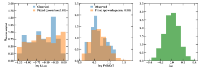
Figure B.1: Modeled probability distribution for $L\mathrm{{}_{bol}}/L\mathrm{{}_{Edd}}$ (left panel) and Fe ii/CaT (middle panel) parameters. Blue distribution correspond to the observed one, while the blue one is obtained via a bootstrap analysis, see Sec.4.5.1. The right panel shows the distribution of the Spearman rank correlation coefficient for 58 randomly selected sources from the distribution in left and middle panel. The number of significant correlations ($\rho_{\rm ran}$ and $p-$val$<0.001$) is below the $3\sigma$ confidence level.

In order to asses any signatures of redshift effects, Fig. B.2 and B.3 show the distributions of the residuals as a function of the redshift for low– and high–$L$ objects. This division is in agreement with low– and high–redshift sources. The median of each distribution (dashed-vertical lines) does not show a significant difference from the zero residual levels and it is not observed a dependency within $2\sigma$ confidence level. This suggests that the relation in figures 3 and 4 are not artificially enhancement by redshift effects.

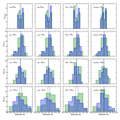
Figure B.2: Distribution of the residuals with respect to the the best fits as a function of redshift for the correlation shown in Fig. 3. In each panel is indicated the analyzed relation. Green distribution correspond to the low–$L$ (and low–$z$) subsample, while blue one draws the high–$L$ (and high–$z$) distributions. Vertical lines indicate the median of each distribution.

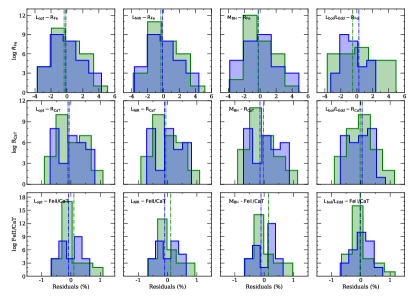
Figure B.3: Same as Fig. B.2, but for correlations shown in Fig. 4.

Appendix C Principal Component Analysis - effect of redundant parameters

The correlation between a variable and a principal component (PC) is used as the coordinates of the variable on the PC. The representation of variables differs from the plot of the observations: The observations are represented by their projections, but the variables are represented by their correlations (Abdi & Williams, 2010). (a) Positively correlated variables are grouped together; (b) negatively correlated variables are positioned on opposite sides of the plot origin (opposed quadrants); and (c) the distance between variables and the origin measures the quality of the variables on the factor map. Variables that are away from the origin are well represented on the factor map.

Figure C.1: Graphical representation of the principal component analysis (PCA) decomposition of our sample (58 sources). The dots represent individual objects on the standardized PC1 - PC2 plane that have variables indicated by the axis labels. The arrows represent the prominence of the variables in the PC1 - PC2 plane. The dashed lines mark the coordinate axes in the PC1 - PC2 plane and the ellipses depict the 95% occupancy of the sources in their respective subsamples. The sample is categorized based on their original source catalogues (see Panda et al., 2020a, for details on the observational sample) - (1) Martínez-Aldama et al. (2015a); (2) Martínez-Aldama et al. (2015b); (3) Persson (1988); (4) Marinello et al. (2016); and (5) PHL1092 (Marinello et al., 2020). LEFT: with $L_{\mathrm{opt}}$; RIGHT: without $L_{\mathrm{opt}}$. The lower panels illustrate the precedence of the first 10 principal components in the form of scree plots.

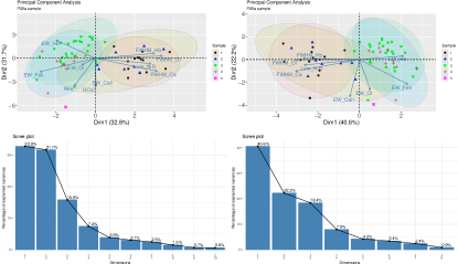
Figure C.2: Similar to Figure C.1. LEFT: with R_FeII and R_CaT; RIGHT: without R_FeII and R_CaT. The lower panels illustrate the precedence of the first 10 principal components in the form of scree plots.

As a first test for the PCA, we consider the aforementioned 11 parameters. Before drawing any definitive conclusions, we wanted to remove parameters that are redundant/uncorrelated. This allows to eliminates noise in the PCA output due to the presence of these redundant/uncorrelated variables. We perform this testing in two steps. In the first step, we analyze the effect of the presence of both optical and NIR luminosity in the PCA run. The optical (at 5100Å) and the NIR (8542Å) luminosities are almost identical for our sample (see bottom-right panel of Figure 2) with a correlation coefficient, r = 0.950 ($p-$value = 6.72$\times 10^{-30}$). This result is snychronous to our PCA (Figure C.1). Here, the factor map for the two cases (with and without optical luminosity) are shown adjacent to each other. At a first glance, the differences in the sources constituting our full sample can be clearly seen. The (3) Persson and (4) Marinello samples (i.e. the low luminosity sources) are similarly oriented in the PC1-PC2 diagram (factor-map), while the high-luminosity sources from the two catalogues from Martinez-Aldama (1 and 2) occupy a separate region in the factor-map. We study these subsamples in more detail in the next section. The corresponding scree plots are similar and highlight the dominance of the first principal component (43% for the case with optical luminosity, and 40.6% for the case without it). The subsequent principal components show similar precedence. We thus make use of only the NIR luminosity henceforth.

The parameters, R_FeII and R_CaT are estimated from the various observations that are tabulated in Table LABEL:tab:table1. These values are estimated from the ratio of the fluxes of the respective emission species (optical Fe ii within the 4434-4684Å and H$\beta$; CaT and H$\beta$, respectively). In our analysis, we use the EWs for the said species which are basically scaled versions of the line fluxes, one that is normalized by the corresponding continuum luminosity (at 5100Å for Fe ii and 8542Å for CaT). Thus, the R_FeII and R_CaT seemingly become redundant in presence of the EWs. We test this effect of redundancy on our sample and the results are presented in Figure C.2. The representation is similar to the Figure C.1. The factor-map on the left panel shows the case where the R_FeII and R_CaT are included in the analysis. Here, the R_CaT vector is completely aligned with the EW(CaT) vector suggesting that the quantity is strongly dependent on this variable itself and is less affected by the EW(H$\beta$). On the other hand, the orientation of the R_FeII vector suggests that the quantity is affected by both EW(Fe ii) and EW(H$\beta$). The corresponding scree plots for the two cases highlight the importance of the noise introduced in the PCA due to the presence of R_FeII and R_CaT. In the case where these variables were used, the dataset is organised such that the two principal components are almost identical (32.8% for PC1 and 31.7% for PC2). This gives a false impression that the dataset is driven by a 2D plane rather than a line. A similar aspect of the optical main sequence being represented as a line or a plane was explored in Wildy et al. (2019). On the other hand, when these two variables are removed and the PCA module is re-run, we see that the dataset is dominated by the variance along the first principal component (40.6%) and the second principal component becomes less important (22.2%). Another effect of the removal of redundant variables is the emergence of other quantities, e.g. EW(O i $\lambda 8446$).

These two tests further confirms that the results of the PCA are dependent on the selection of the sample and the chosen properties (Kuraszkiewicz et al., 2009).

Appendix D Principal Component Analysis. Low- and high-luminosity samples

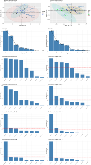
Figure D.1: Same as Figure 5. LEFT: low-luminosity sample (log $L_{\mathrm{opt}}$ $\leq$ 44.49 erg s^-1). RIGHT: high-luminosity sample (log $L_{\mathrm{opt}}$ $>$ 44.49 erg s^-1).

Taking note from the previous runs and the heterogeneity present in our sample, we now separate the full sample into two subsamples based on the median of the optical luminosity (at 5100 Å) of the distribution, i.e. log $L_{\mathrm{opt}}$ = 44.49 erg s^-1 (Sec. 4.3.3), which gives 29 sources in each case. We then perform the PCA on each of the subsamples (low $L_{\rm opt}$ and high $L_{\rm opt}$) and illustrate the results in the left and right columns of Figure D.1, respectively.

D.1 Low-luminosity subsample

For the low-luminosity sample, the sources belong to the Persson (19/25) and Marinello (10/10) samples, and the Marinello sample is almost enclosed within the Persson sample in the factor-map. The corresponding scree plot shows the dominance of the primary and secondary principal components (41.1% and 30.1%), suggesting that the sample seems to be driven majorly by the combination of the two components that can explain 71.2% of the variance in the dataset. Accounting for the subsequent two principal components, 90.6% of the total variation in the dataset can be explained in this case.

First principal component: Going back to the factor-map, we find that the vectors corresponding to the FWHMs of H$\beta$ and O i $\lambda 8446$, EW_Hβ are co-aligned, with the FWHM vectors having almost similar magnitudes. These two FWHM vectors are also the major contributors to the variance along the primary principal component (see third panel on the middle column of Figure 5). For the primary principal component, the EW of O i $\lambda 8446$ follows after these two FWHMs, which then is followed by the NIR luminosity.

Second principal component: The factor-map highlights the prevalence of the EW_CaTfollowed by the FWHM_CaTand the EW_FeIIṪhis trend is also seen in the contributions to the second principal component and supports our original conclusion that the two species, Fe ii and CaT are similar in terms of their excitation and line emissivities (see fourth panel on the middle of Figure 5). We expect that the FWHM_FeII would show similar behaviour, likewise of FWHM_CaT (as shown in Marinello et al., 2016, where the authors show an almost perfect correlation between the Fe ii emission at 1 $\mu$m and CaT) strengthening the inferences from the photoionization modelling (Panda et al., 2020a; Panda, 2020). This needs to be tested with a larger, of higher S/N and more-complete sample in the future.

Third and fourth principal components: The third and fourth principal components further contribute to 19.4% of the total variance in the dataset. The third PC is singularly dominated by the EW_Hβ with a minor contribution from EW_CaTand FWHM_Hβ}. Similarly, the fourth PC is mainly driven by the FWHM_CaT and only a minor contribution from EW of O i $\lambda 8446$.

D.2 high-luminosity subsample

For the high-luminosity sample, the sources belong to the Persson (6/25), Marinello (PHL1092) samples, and all of Martinez-Aldama’s sources. The 6 sources from Persson (Mrk304, Mrk509, IZw1, Mrk478, VIIZw118 and 3C273) and PHL1092, outline around the 95% confidence limit of the Martinez-Aldama’s sample shown with the ellipses on the factor-map (top-right panel in Figure 5). This points towards the homogeneity in the subsample as opposed to the earlier scenario when all the sources were bunched together. The corresponding scree plot shows the dominance of the primary and secondary principal components (42.7% and 22.5%), suggesting that the high-luminosity sample behaves similar to the low-luminosity case. Likewise to the low-luminosity case, accounting for the subsequent two principal components (PC3 and PC4), 91.4% of the total variation in the high-luminosity dataset can be explained.

First principal component: Compared to the low-luminosity case, the FWHM of O i $\lambda 8446$ is still the primary dominant driver of the the primary PC, followed by the EW_FeII  FWHM_Hβ and FWHM_CaT. The EW_FeII dominates in the negative space of the PC1.

Second principal component: The primary contributor to this PC is still EW_CaT, but in contrast to the corresponding PC for the low-luminosity case, the EW_FeII is rather below the significance threshold in this case. Other significant contributors are the EW_Hβ followed by the FWHM_CaT.

Third and fourth principal components: The third and fourth principal components further contribute to 26.2% (earlier this was 19.4% for the low-luminosity case) of the total variance in the dataset. The third PC is dominated by the EW_OI with contribution from EW_Hβ. Whereas, the fourth PC is singularly driven by the NIR luminosity.

D.3 Correlations between the principal eigenvectors and observed/derived parameters for the subsamples

Figure D.2: For the PC1, there are significant positive correlations for both the subsamples, especially, with respect to FWHM_Hβ (low-luminosity: $\rho$=0.669, $p$=7.37$\times 10^{-5}$; high-luminosity: $\rho$=0.76, $p$=1.73$\times 10^{-6}$) and FWHM_OI (low-luminosity: $\rho$=0.728, $p$=7.65$\times 10^{-6}$; high-luminosity: $\rho$=0.884, $p$=2.1$\times 10^{-10}$). This is highlighted by the strong correlation between the PC1 and the black hole mass which is obtained and explained in Figure D.3 as the FWHM_Hβ is incorporated to estimate the black hole mass. A strong positive correlation is obtained for FWHM_CaT ($\rho$=0.85, $p$=3.94$\times 10^{-8}$) for the high luminosity subsample. The EW_Hβ correlation with PC1 behaves differently for the low-luminosity ($\rho$=0.736, $p$=5.46$\times 10^{-6}$) and the high-luminosity ($\rho$=-0.694, $p$=2.93$\times 10^{-5}$) samples. The low-luminosity sample follows the trend of the full sample in this case. For EW_OI, significant correlation is noted only for the low-luminosity case ($\rho$=0.871, $p$=8.11$\times 10^{-10}$). For EW_FeII, significant anti-correlation is noted only for the high-luminosity case ($\rho$=-0.681, $p$=4.73$\times 10^{-5}$) . For PC2, we have two significant correlations for the low-luminosity case - for EW_CaT ($\rho$=0.855, $p$=3.57$\times 10^{-9}$) and EW_FeII ($\rho$=0.66, $p$=9.88$\times 10^{-5}$). Additionally, there is a correlation obtained for the EW_CaT ($\rho$=0.86, $p$=2.3$\times 10^{-9}$) for the high-luminosity case. For PC3, a significant anti-correlation is observed for the low-luminosity case’s EW_Hβ ($\rho$=-0.743, $p$=3.87$\times 10^{-6}$) and a significant correlation for the high luminosity case’s EW_OI ($\rho$=0.83, $p$=2.57$\times 10^{-8}$). There is a single significant (anti-)correlation observed for PC4, i.e. versus FWHM_CaT ($\rho$=-0.699, $p$=6.02$\times 10^{-4}$).

Figure D.3: The strongest and only correlation in the subsamples for the PC1 are with respect to the black hole mass - for the low-luminosity sample, the correlation is relatively stronger ($\rho$=0.701, p=2.24$\times 10^{-5}$) compared to the high-luminosity sample ($\rho$=0.662, $p$=9.16$\times 10^{-5}$). For PC2, significant correlations are obtained only for R_FeII and R_CaT cases. For the low-luminosity sample, the correlations of PC2 versus R_FeII ($\rho$=0.698, $p$=2.6$\times 10^{-5}$) and versus R_CaT ($\rho$=0.65, $p$=1.34$\times 10^{-4}$), while for the high-luminosity sample, the correlations of PC2 versus R_FeII ($\rho$=0.669, $p$=7.26$\times 10^{-5}$) and versus R_CaT ($\rho$=0.838, $p$=1.46$\times 10^{-8}$). This further corroborates the strong connection between these two parameters from our past results obtained in Paper-1 and those obtained from the PCA analysis of the full sample in this paper. There are no significant correlations with respect to PC3. The only significant (anti-)correlation with respect to PC4 is obtained for $L\mathrm{{}_{Edd}}$ in high-luminosity sample ($\rho$=-0.693, $p$=3.13$\times 10^{-5}$).

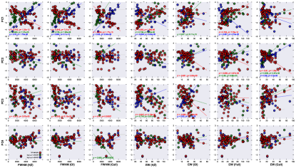
Figure D.2: Correlation matrix showing dependence of the first four PCA vectors’ loadings versus the physical parameters (observed) for our sample. The sample is divided into low luminosity (green dots) and high luminosity (blue dots) subsamples based on the median value of the sample’s optical luminosity distribution, i.e. at 44.49 erg s^-1 (see Appendix D). The full sample is shown in red dots. The Spearman’s rank correlation coefficient ($\rho$) and the $p-$value are reported for the correlations whenever $p$-value $<$ 0.001. The OLS fits for each sample is shown using dashed lines using their respective color.

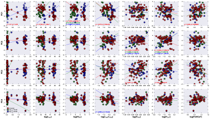
Figure D.3: Correlation matrix showing dependence of the first four PCA vectors’ loadings versus the physical parameters (derived) for our sample. The colors for the data-points are identical to that shown previously in Figure D.2. The Spearman’s rank correlation coefficients ($\rho$) and the $p-$values are reported for the correlations whenever $p-$value $<$ 0.001. The OLS fits for each sample is shown using dashed lines using their respective color.

References

- Abdi & Williams (2010) Abdi, H., & Williams, L. J. 2010, WIREs Computational Statistics, 2, 433, doi: 10.1002/wics.101
- Bachev et al. (2004) Bachev, R., Marziani, P., Sulentic, J. W., et al. 2004, The Astrophysical Journal, 617, 171, doi: 10.1086/425210
- Baldwin (1977) Baldwin, J. A. 1977, ApJ, 214, 679, doi: 10.1086/155294
- Baldwin et al. (1978) Baldwin, J. A., Burke, W. L., Gaskell, C. M., & Wampler, E. J. 1978, Nature, 273, 431, doi: 10.1038/273431a0
- Baldwin et al. (2004) Baldwin, J. A., Ferland, G. J., Korista, K. T., Hamann, F., & LaCluyzé, A. 2004, ApJ, 615, 610, doi: 10.1086/424683
- Baskin & Laor (2004) Baskin, A., & Laor, A. 2004, Monthly Notices of the Royal Astronomical Society, 350, L31, doi: 10.1111/j.1365-2966.2004.07833.x
- Bentz et al. (2013) Bentz, M. C., Denney, K. D., Grier, C. J., et al. 2013, ApJ, 767, 149, doi: 10.1088/0004-637X/767/2/149
- Bessell (1990) Bessell, M. S. 1990, PASP, 102, 1181, doi: 10.1086/132749
- Bizyaev et al. (2019) Bizyaev, D., Chen, Y.-M., Shi, Y., et al. 2019, ApJ, 882, 145, doi: 10.3847/1538-4357/ab3406
- Boroson & Green (1992) Boroson, T. A., & Green, R. F. 1992, ApJS, 80, 109, doi: 10.1086/191661
- Collin & Joly (2000) Collin, S., & Joly, M. 2000, New A Rev., 44, 531, doi: 10.1016/S1387-6473(00)00093-2
- Collin et al. (2006) Collin, S., Kawaguchi, T., Peterson, B. M., & Vestergaard, M. 2006, A&A, 456, 75, doi: 10.1051/0004-6361:20064878
- Collin-Souffrin et al. (1988) Collin-Souffrin, S., Dyson, J. E., McDowell, J. C., & Perry, J. J. 1988, MNRAS, 232, 539, doi: 10.1093/mnras/232.3.539
- de Bruyn & Sargent (1978) de Bruyn, A. G., & Sargent, W. L. W. 1978, AJ, 83, 1257, doi: 10.1086/112320
- De Rosa et al. (2014) De Rosa, G., Venemans, B. P., Decarli, R., et al. 2014, ApJ, 790, 145, doi: 10.1088/0004-637X/790/2/145
- Devereux (2018) Devereux, N. 2018, MNRAS, 473, 2930, doi: 10.1093/mnras/stx2537
- Dietrich et al. (2003) Dietrich, M., Hamann, F., Appenzeller, I., & Vestergaard, M. 2003, ApJ, 596, 817, doi: 10.1086/378045
- Dietrich et al. (2002) Dietrich, M., Hamann, F., Shields, J. C., et al. 2002, ApJ, 581, 912, doi: 10.1086/344410
- Dong et al. (2011) Dong, X.-B., Wang, J.-G., Ho, L. C., et al. 2011, ApJ, 736, 86, doi: 10.1088/0004-637X/736/2/86
- Dong et al. (2009) Dong, X.-B., Wang, T.-G., Wang, J.-G., et al. 2009, The Astrophysical Journal, 703, L1, doi: 10.1088/0004-637x/703/1/l1
- Du & Wang (2019) Du, P., & Wang, J.-M. 2019, ApJ, 886, 42, doi: 10.3847/1538-4357/ab4908
- Dultzin-Hacyan et al. (1999) Dultzin-Hacyan, D., Taniguchi, Y., & Uranga, L. 1999, in Astronomical Society of the Pacific Conference Series, Vol. 175, Structure and Kinematics of Quasar Broad Line Regions, ed. C. M. Gaskell, W. N. Brandt, M. Dietrich, D. Dultzin-Hacyan, & M. Eracleous, 303
- Efron & Tibshirani (1993) Efron, B., & Tibshirani, R. J. 1993, An Introduction to the Bootstrap, Monographs on Statistics and Applied Probability No. 57 (Boca Raton, Florida, USA: Chapman & Hall/CRC)
- Ferland & Persson (1989) Ferland, G. J., & Persson, S. E. 1989, ApJ, 347, 656, doi: 10.1086/168156
- Ferland et al. (2017) Ferland, G. J., Chatzikos, M., Guzmán, F., et al. 2017, Rev. Mexicana Astron. Astrofis., 53, 385. https://arxiv.org/abs/1705.10877
- Garcia-Rissmann et al. (2012) Garcia-Rissmann, A., Rodríguez-Ardila, A., Sigut, T. A. A., & Pradhan, A. K. 2012, ApJ, 751, 7, doi: 10.1088/0004-637X/751/1/7
- Garcia-Rissmann et al. (2005) Garcia-Rissmann, A., Vega, L. R., Asari, N. V., et al. 2005, MNRAS, 359, 765, doi: 10.1111/j.1365-2966.2005.08957.x
- Green et al. (2001) Green, P. J., Forster, K., & Kuraszkiewicz, J. 2001, The Astrophysical Journal, 556, 727, doi: 10.1086/321600
- Hamann & Ferland (1992) Hamann, F., & Ferland, G. 1992, ApJ, 391, L53, doi: 10.1086/186397
- Hamann & Ferland (1993a) —. 1993a, ApJ, 418, 11, doi: 10.1086/173366
- Hamann & Ferland (1993b) —. 1993b, ApJ, 418, 11, doi: 10.1086/173366
- Hamann & Ferland (1999) —. 1999, ARA&A, 37, 487, doi: 10.1146/annurev.astro.37.1.487
- Horne et al. (2020) Horne, K., De Rosa, G., Peterson, B. M., et al. 2020, arXiv e-prints, arXiv:2003.01448. https://arxiv.org/abs/2003.01448
- Hunter (2007) Hunter, J. D. 2007, Computing in Science and Engineering, 9, 90, doi: 10.1109/MCSE.2007.55
- Jolliffe (2011) Jolliffe, I. 2011, Principal Component Analysis, ed. M. Lovric (Berlin, Heidelberg: Springer Berlin Heidelberg), 1094–1096, doi: 10.1007/978-3-642-04898-2_455
- Joly (1987) Joly, M. 1987, A&A, 184, 33
- Joly (1989) —. 1989, A&A, 208, 47
- Kaiser (1961) Kaiser, H. F. 1961, British Journal of Statistical Psychology, 14, 1, doi: 10.1111/j.2044-8317.1961.tb00061.x
- Korista et al. (1998) Korista, K., Baldwin, J., & Ferland, G. 1998, ApJ, 507, 24, doi: 10.1086/306321
- Korista et al. (1997) Korista, K., Baldwin, J., Ferland, G., & Verner, D. 1997, ApJS, 108, 401, doi: 10.1086/312966
- Koski (1978) Koski, A. T. 1978, ApJ, 223, 56, doi: 10.1086/156235
- Krawczyk et al. (2013) Krawczyk, C. M., Richards, G. T., Mehta, S. S., et al. 2013, ApJS, 206, 4, doi: 10.1088/0067-0049/206/1/4
- Kunth & Sargent (1979) Kunth, D., & Sargent, W. L. W. 1979, A&A, 76, 50
- Kuraszkiewicz et al. (2009) Kuraszkiewicz, J., Wilkes, B. J., Schmidt, G., et al. 2009, ApJ, 692, 1180, doi: 10.1088/0004-637X/692/2/1180
- Lusso & Risaliti (2016) Lusso, E., & Risaliti, G. 2016, ApJ, 819, 154, doi: 10.3847/0004-637X/819/2/154
- Madau & Dickinson (2014) Madau, P., & Dickinson, M. 2014, Annual Review of Astronomy and Astrophysics, 52, 415, doi: 10.1146/annurev-astro-081811-125615
- Marconi et al. (2004) Marconi, A., Risaliti, G., Gilli, R., et al. 2004, MNRAS, 351, 169, doi: 10.1111/j.1365-2966.2004.07765.x
- Marinello et al. (2016) Marinello, M., Rodríguez-Ardila, A., Garcia-Rissmann, A., Sigut, T. A. A., & Pradhan, A. K. 2016, ApJ, 820, 116, doi: 10.3847/0004-637X/820/2/116
- Marinello et al. (2020) Marinello, M., Rodríguez-Ardila, A., Marziani, P., Sigut, A., & Pradhan, A. 2020, MNRAS, 494, 4187, doi: 10.1093/mnras/staa934