Least resolved trees for two-colored best match graphs

Abstract

2-colored best match graphs (2-BMGs) form a subclass of sink-free bi-transitive graphs that appears in phylogenetic combinatorics. There, 2-BMGs describe evolutionarily most closely related genes between a pair of species. They are explained by a unique least resolved tree (LRT). Introducing the concept of support vertices we derive an $O(|V|+|E|\log^{2}|V|)$-time algorithm to recognize 2-BMGs and to construct its LRT. The approach can be extended to also recognize binary-explainable 2-BMGs with the same complexity. An empirical comparison emphasizes the efficiency of the new algorithm.

1 Introduction

Best match graphs recently have been introduced in phylogenetic combinatorics to formalize the notion of a gene $y$ in species $2$ being an evolutionary closest relative of a gene $x$ in species $1$, i.e., $y$ is a best match for $x$ [5]. The best matches between genes of two species form a bipartite directed graph, the 2-colored best match graph or 2-BMG, that is determined by the phylogenetic tree describing the evolution of the genes. 2-BMGs are characterized by four local properties [5, 8] that relate them to previously studied classes of digraphs:

Definition 1.

A bipartite digraph $\mathaccent 382{G}=(L,E)$ is a 2-BMG if it satisfies

(N0)

Every vertex has at least one out-neighbor, i.e., $\mathaccent 382{G}$ is sink-free.

(N1)

If $u$ and $v$ are two independent vertices, then there exist no vertices $w$ and $t$ such that $(u,t),(v,w),(t,w)\in E$.

(N2)

For any four vertices $u_{1},u_{2},v_{1},v_{2}$ with $(u_{1},v_{1}),(v_{1},u_{2}),(u_{2},v_{2})\in E$ we have $(u_{1},v_{2})\in E$, i.e., $\mathaccent 382{G}$ is bi-transitive.

(N3)

For any two vertices $u$ and $v$ with a common out-neighbor, if there exists no vertex $w$ such that either $(u,w),(w,v)\in E$, or $(v,w),(w,u)\in E$, then $u$ and $v$ have the same in-neighbors and either all out-neighbors of $u$ are also out-neighbors of $v$ or all out-neighbors of $v$ are also out-neighbors of $u$.

Sink-free graphs have appeared in particular in the context of graph semigroups [1] and graph orientation problems [3]. Bi-transitive graphs were introduced in [4] in the context of oriented bipartite graphs and investigated in more detail in [8, 7]. The class of graphs satisfying (N1), (N2), and (N3) are characterized by a system of forbidden induced subgraphs [12], see Thm. 2 below.

In general, best match graphs (BMGs) are defined as vertex-colored digraphs $(\mathaccent 382{G},\sigma)$, where the vertex coloring $\sigma$ assigns to each gene $x$ the species $\sigma(x)$ in which it resides. The subgraphs of a BMG induced by vertices of two distinct colors form a 2-BMG. Note that in this context the vertex coloring is assigned a priori, while Def. 1 induces a coloring that is unique only up to relabeling of the colors independently on each (weakly) connected component of $\mathaccent 382{G}$. For each BMG $(\mathaccent 382{G},\sigma)$, there is a unique least resolved leaf-colored tree $(T^{*},\sigma)$ with leaves corresponding to the vertices of $(\mathaccent 382{G},\sigma)$ such that the arcs in $(\mathaccent 382{G},\sigma)$ are the best matches w.r.t. $(T^{*},\sigma)$ (cf. Def. 2 below). Fig. 1 shows an example for a 2-BMG together with its least resolved tree. Using certain sets of rooted triples that can be inferred from the 2-colored induced subgraphs of $(\mathaccent 382{G},\sigma)$ with three vertices, it is possible to determine whether $(G,\sigma)$ is a BMG in polynomial time and, if so, to construct the least resolved tree $(T^{*},\sigma)$ [5, 9]. This work also describes $O(|V|^{3})$-time algorithms for the recognition of 2-BMGs and the construction of the LRT for a given 2-BMG.

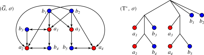
Figure 1: Example for a 2-BMG $(\mathaccent 382{G},\sigma)$ and its explaining least resolved tree $(T^{*},\sigma)$.

In this contribution, we derive an alternative characterization of 2-BMGs that avoids the use of rooted triples. This will give rise to an alternative, efficient algorithm for the recognition of 2-BMGs and the construction of the least resolved tree. The contribution is organized as follows: In Sec. 2, we introduce the necessary notation and review some results from the published literature that are needed later on. Sec. 3 is concerned with a more detailed analysis of the least resolved trees (LRTs) of BMGs with an arbitrary number of colors. We then turn to the peculiar properties of the LRTs of 2-BMGs in Sec. 4. To this end, we introduce the concept of “support leaves” that uniquely determine the LRT. The main result of this section is Thm. 4, which shows that the support leaves of the root can be identified directly in the 2-BMG. In Sec. 5, we then turn Thm. 4 into an efficient algorithm for recognizing 2-BMGs and constructing their LRTs. Computational experiments demonstrate the performance gain in practise. In Sec. 6 we extend the algorithmic approach to binary-explainable 2-BMGs, a subclass that features an additional forbidden induced subgraph.

2 Preliminaries

Let $T=(V,E)$ be a tree with root $\rho$ and leaf set $L\coloneqq L(T)\subset V$. The set of inner vertices of $T$ is $V^{0}(T)\coloneqq V\setminus L$, in particular $\rho$ is an inner vertex. An edge $e=uv\in E(T)$ is called an inner edge of $T$ if $u$ and $v$ are both inner vertices. Otherwise it is called an outer edge. We consider leaf-colored trees $(T,\sigma)$ and write $\sigma(L^{\prime})\coloneqq\{\sigma(v)\mid v\in L^{\prime}\}$ for subsets $L^{\prime}\subseteq L$. A vertex $u\in V$ is an ancestor of $v\in V$ in $T$, in symbols $v\preceq_{T}u$, if $u$ lies on the path from $\rho$ to $v$. For the edges $uv\in E(T)$ we use the convention that $uv\in E$, $v\prec_{T}u$, $v$ is a child of $u$. We write $\operatorname{child}_{T}(u)$ for the set of children of $u$ in $T$ and $T(u)$ for the subtree of $T$ rooted in $u$. The least common ancestor $\operatorname{lca}_{T}(A)$ is the unique $\preceq_{T}$-smallest vertex that is an ancestor of all genes in $A$. Writing $\operatorname{lca}_{T}(x,y)\coloneqq\operatorname{lca}_{T}(\{x,y\})$, we have

Definition 2.

Let $(T,\sigma)$ be a leaf-colored tree. A leaf $y\in L(T)$ is a best match of the leaf $x\in L(T)$ if $\sigma(x)\neq\sigma(y)$ and $\operatorname{lca}(x,y)\preceq_{T}\operatorname{lca}(x,y^{\prime})$ holds for all leaves $y^{\prime}$ of color $\sigma(y^{\prime})=\sigma(y)$.

Given $(T,\sigma)$, the graph $\mathaccent 382{G}(T,\sigma)=(V,E)$ with vertex set $V=L(T)$, vertex coloring $\sigma$, and with arcs $(x,y)\in E$ if and only if $y$ is a best match of $x$ w.r.t. $(T,\sigma)$ is called the best match graph (BMG) of $(T,\sigma)$ [5].

Definition 3.

An arbitrary vertex-colored graph $(\mathaccent 382{G},\sigma)$ is a best match graph (BMG) if there exists a leaf-colored tree $(T,\sigma)$ such that $(\mathaccent 382{G},\sigma)=\mathaccent 382{G}(T,\sigma)$. In this case, we say that $(T,\sigma)$ explains $(\mathaccent 382{G},\sigma)$.

Theorem 1 ([5], Thm. 9).

If $(\mathaccent 382{G},\sigma)$ is a BMG, then there is a unique least-resolved tree $(T,\sigma)$ that explains $(\mathaccent 382{G},\sigma)$.

We say that $(\mathaccent 382{G},\sigma)$ is an $\ell$-BMG if $\sigma:V(\mathaccent 382{G})\to S$ is surjective and $|S|=\ell$. Given a directed graph $\mathaccent 382{G}=(V,E)$ we denote the set of out-neighbors of a vertex $x\in V$ by $N(x)\coloneqq\{y\in V|(x,y)\in E(\mathaccent 382{G})\}$ and the out-degree $|N(x)|$ of $x$ by $\operatorname{outdeg}(x)$. Similarly, $N^{-}(x)\coloneqq\{y\in V|(y,x)\in E(\mathaccent 382{G})\}$ denotes the set of in-neighbors. By construction, the coloring $\sigma$ of a BMGs $(\mathaccent 382{G},\sigma)$ is proper, i.e., $x\in N(y)$ implies $\sigma(x)\neq\sigma(y)$, and there is at least one best match of $x$ for every color $s\in\sigma(V)\setminus\{\sigma(x)\}$. In particular, therefore, we have $N(x)\neq\emptyset$ for every 2-BMG, i.e., every 2-BMG is sink-free. Note that BMGs will in general have sources, i.e., $N^{-}(x)$ may be empty. We write $\mathaccent 382{G}[W]$ for the subgraph of $\mathaccent 382{G}=(V,E)$ induced by $W\subseteq V$ and $\mathaccent 382{G}-W$ for $\mathaccent 382{G}[V\setminus W]$. A directed graph is (weakly) connected if its underling undirected graph is connected. A connected component is a maximal connected subgraph of $\mathaccent 382{G}$.

Following [13] we say that $T^{\prime}$ is displayed by $T$, in symbols $T^{\prime}\leq T$, if the tree $T^{\prime}$ can be obtained from a subtree of $T$ by contraction of edges. For leaf-colored trees we say that $(T,\sigma)$ displays or is a refinement of $(T^{\prime},\sigma^{\prime})$, whenever $T^{\prime}\leq T$ and $\sigma(v)=\sigma^{\prime}(v)$ for all $v\in L(T^{\prime})$.

Definition 4.

An edge $e\in E(T)$ is redundant with respect to $\mathaccent 382{G}(T,\sigma)$ if the tree $T_{e}$ obtained by contracting the edge $e$ satisfies $\mathaccent 382{G}(T_{e},\sigma)=\mathaccent 382{G}(T,\sigma)$.

We will need the following characterization of redundant edges:

Lemma 1 ([11], Lemma 2.10).

Let $(\mathaccent 382{G},\sigma)$ be a BMG explained by a tree $(T,\sigma)$. The edge $e=uv$ in $(T,\sigma)$ is redundant w.r.t. $(\mathaccent 382{G},\sigma)$ if and only if (i) $e$ is an inner edge of $T$ and (ii) there is no arc $(a,b)\in E(\mathaccent 382{G})$ such that $\operatorname{lca}_{T}(a,b)=v$ and $\sigma(b)\in\sigma(L(T(u))\setminus L(T(v)))$.

In the following we will frequently need the restriction of the coloring $\sigma$ on $\mathaccent 382{G}$ or $L(T)$ to a subset of vertices or leaves. Since in situations like $(G_{i},\sigma_{|V(G_{i})})$ the set to which $\sigma$ is restricted is clear, we will write $\sigma_{|.}$ to keep the notation less cluttered.

BMGs can also be understood in terms of their connected components:

Proposition 1 ([5], Prop. 1).

A digraph $(\mathaccent 382{G},\sigma)$ is an $\ell$-BMG if and only if all its connected components are $\ell$-BMGs.

As a simple consequence of Prop. 1 and by definition of $\ell$-BMGs, all connected components $(G_{i},\sigma_{|.})$ and $(G_{j},\sigma_{|.})$ of an $\ell$-BMG satisfy $\sigma(V(G_{i}))=\sigma(V(G_{j}))$ and $|\sigma(V(G_{j}))|=\ell$. For our purposes it will also be important to relate the structure of a tree $(T,\sigma)$ to the connectedness of the BMG $\mathaccent 382{G}(T,\sigma)$ that it explains.

Proposition 2 ([5], Thm. 1).

Let $(T,\sigma)$ be a leaf-labeled tree and $\mathaccent 382{G}(T,\sigma)$ its BMG. Then $\mathaccent 382{G}(T,\sigma)$ is connected if and only if there is a child $v$ of the root $\rho$ such that $\sigma(L(T(v)))\neq\sigma(L(T))$. Furthermore, if $\mathaccent 382{G}(T,\sigma)$ is not connected, then for every connected component $\mathaccent 382{G}_{i}$ of $\mathaccent 382{G}(T,\sigma)$ there is a child $v$ of the root $\rho$ such that $V(G_{i})\subseteq L(T(v))$.

Moreover, 2-BMGs can be characterized by three types of forbidden subgraphs [12]. To this end we will need the following classes of small bipartite graphs:

Definition 5 (F1-, F2-, and F3-graphs).

(F1)

A properly 2-colored graph on four distinct vertices $V=\{x_{1},x_{2},y_{1},y_{2}\}$ with coloring $\sigma(x_{1})=\sigma(x_{2})\neq\sigma(y_{1})=\sigma(y_{2})$ is an F1-graph if $(x_{1},y_{1}),(y_{2},x_{2}),(y_{1},x_{2})\in E$ and $(x_{1},y_{2}),(y_{2},x_{1})\notin E$.

(F2)

A properly 2-colored graph on four distinct vertices $V=\{x_{1},x_{2},y_{1},y_{2}\}$ with coloring $\sigma(x_{1})=\sigma(x_{2})\neq\sigma(y_{1})=\sigma(y_{2})$ is an F2-graph if $(x_{1},y_{1}),(y_{1},x_{2}),(x_{2},y_{2})\in E$ and $(x_{1},y_{2})\notin E$.

(F3)

A properly 2-colored graph on five distinct vertices $V=\{x_{1},x_{2},y_{1},y_{2},y_{3}\}$ with coloring $\sigma(x_{1})=\sigma(x_{2})\neq\sigma(y_{1})=\sigma(y_{2})=\sigma(y_{3})$ is an F3-graph if
$(x_{1},y_{1}),(x_{2},y_{2}),(x_{1},y_{3}),(x_{2},y_{3})\in E$ and $(x_{1},y_{2}),(x_{2},y_{1})\notin E$.

Theorem 2 ([12], Thm. 3.4).

A properly 2-colored graph is a 2-BMG if and only if it is sink-free and does not contain an induced F1-, F2-, or F3-graph.

As noted in [12], the forbidden induced F1-, F2-, and F3-subgraphs characterize exactly the class of bipartite directed graphs satisfying the Axioms (N1), (N2), and (N3) mentioned in the introduction.

Although we aim at avoiding the use of triples in the final results, we will need them during our discussion. A triple $ab|c$ is a rooted tree $t$ on three pairwise distinct vertices $\{a,b,c\}$ such that $\operatorname{lca}_{t}(a,b)\prec_{t}\operatorname{lca}_{t}(a,c)=\operatorname{lca}_{t}(b,c)=\rho$, where $\rho$ denotes the root of $t$. A set $\mathscr{R}$ of triples is consistent if there is a tree $T$ that displays all triples in $\mathscr{R}$. Given a vertex-colored graph $(\mathaccent 382{G},\sigma)$, we define its set of informative triples [5, 11] as

$$\mathscr{R}(\mathaccent 382{G},\sigma)\coloneqq\left\{ab|b^{\prime}\colon\sigma(a)\neq\sigma(b)=\sigma(b^{\prime}),\,(a,b)\in E(\mathaccent 382{G});(a,b^{\prime})\notin E(\mathaccent 382{G})\right\}.$$ (1)

Lemma 2 ([11], Lemma 2.8 and 2.9).

If $(\mathaccent 382{G},\sigma)$ is a BMG, then every tree $(T,\sigma)$ that explains $(\mathaccent 382{G},\sigma)$ displays all triples $t\in\mathscr{R}(\mathaccent 382{G},\sigma)$.
Moreover, if the triples $ab|b^{\prime}$ and $cb^{\prime}|b$ are informative for $(\mathaccent 382{G},\sigma)$, then every tree $(T,\sigma)$ that explains $(\mathaccent 382{G},\sigma)$ contains two distinct children $v_{1},v_{2}\in\operatorname{child}_{T}(\operatorname{lca}_{T}(a,c))$ such that $a,b\prec_{T}v_{1}$ and $b^{\prime},c\prec_{T}v_{2}$.

Observation 3.

Let $(T,\sigma)$ be a tree explaining the BMG $(\mathaccent 382{G},\sigma)$, and $v\in V(T)$ a vertex such that $\sigma(L(T(v)))=\sigma(L(T))$. Then $(a,b)\in E(\mathaccent 382{G})$ and $a\in L(T(v))$ implies $b\in L(T(v))$.

Finally, there is a close connection between subtrees of $T$ and subgraphs of $\mathaccent 382{G}(T,\sigma)$. We have

Lemma 3 ([9], Lemma 22 and 23).

Let $(T,\sigma)$ be a tree explaining an BMG $(\mathaccent 382{G},\sigma)$. Then $\mathaccent 382{G}(T(u),\sigma_{|.})=(\mathaccent 382{G}[L(T(u))],\sigma_{|.})$ holds for every $u\in V(T)$. Moreover, if $(T,\sigma)$ is least resolved for $(\mathaccent 382{G},\sigma)$, then the subtree $T(u)$ is least resolved for $\mathaccent 382{G}(T(u),\sigma_{|.})$.

3 Properties of Least Resolved Trees

In this short section we derive some helpful properties of LRTs which we will use repeatedly throughout this work.

Lemma 4.

Let $(\mathaccent 382{G},\sigma)$ be a BMG and $(T,\sigma)$ its least resolved tree. Then the BMG $\mathaccent 382{G}(T(v),\sigma_{|.})$ is connected for every $v\in V(T)$ with $v\prec_{T}\rho_{T}$.

Proof.

By Lemma 3, $\mathaccent 382{G}(T(v),\sigma_{|.})$ is a BMG. First observe that the BMG $\mathaccent 382{G}(T(v),\sigma_{|.})$ is trivially connected if $v$ is a leaf. Now let $v\prec_{T}\rho_{T}$ be an arbitrary inner vertex of $T$. Thus, there exists a vertex $u\succ_{T}v$ such that $uv$ is an inner edge. Since $(T,\sigma)$ is least resolved, it does not contain any redundant edges. Hence, by contraposition of Lemma 1, there is an arc $(a,b)\in E(\mathaccent 382{G})$ such that $\operatorname{lca}_{T}(a,b)=v$ and $\sigma(b)\in\sigma(L(T(u))\setminus L(T(v)))$. Since $a,b\in L(T(v))$, Lemma 3 implies that $(a,b)$ is also an arc in $\mathaccent 382{G}(T(v),\sigma_{|.})$. Moreover, $\operatorname{lca}_{T(v)}(a,b)=v$ clearly also holds in the subtree rooted at $v$. Now consider the child $w\in\operatorname{child}_{T(v)}(v)$ such that $a\preceq_{T(v)}w$. There cannot be a leaf $b^{\prime}\in L(T(w))$ with $\sigma(b^{\prime})=\sigma(b)$ since otherwise $\operatorname{lca}_{T(v)}(a,b^{\prime})\preceq_{T(v)}w\prec_{T(v)}v$ would contradict that $(a,b)$ is an arc in $\mathaccent 382{G}(T(v),\sigma_{|.})$. Thus $\sigma(b)\notin\sigma(L(T(w)))$. Since $\sigma(b)\in\sigma(L(T(v)))$, we thus conclude $\sigma(L(T(w)))\neq\sigma(L(T(v)))$. The latter together with Prop. 2 implies that $\mathaccent 382{G}(T(v),\sigma_{|.})$ is connected. ∎

The converse of Lemma 4, however, is not true, i.e., a tree $(T,\sigma)$ for which $\mathaccent 382{G}(T(v),\sigma_{|.})$ is connected for every $v\in V(T)$ with $v\prec_{T}\rho_{T}$ is not necessarily least resolved. To see this, consider the caterpillar tree $(T,\sigma)$ given by $(x^{\prime\prime},(x^{\prime},(x,y)))$ with $\sigma(x)=\sigma(x^{\prime})=\sigma(x^{\prime\prime})\neq\sigma(y)$ and $u=\operatorname{lca}_{T}(x,x^{\prime})$. It is an easy task to verify that the BMG of each subtree of $T$ is connected. However, the edge $\rho_{T}u$ is redundant.

Lemma 5.

Let $(T,\sigma)$ be the least resolved tree of some BMG $(\mathaccent 382{G},\sigma)$. Then every vertex $v\prec_{T}\rho_{T}$ with $|\sigma(L(T(v)))|=1$ is a leaf.

Proof.

Let $v\prec_{T}\rho_{T}$ with $|\sigma(L(T(v)))|=1$ and assume, for contradiction, that $v$ is not a leaf. Hence, $|L(T(v))|>1$. By Lemma 3 $\mathaccent 382{G}(T(v),\sigma_{|.})$ is a BMG and, therefore, properly colored. But then $\mathaccent 382{G}(T(v),\sigma_{|.})$ is disconnected; a contradiction to Lemma 4. ∎

As a consequence we find

Corollary 1.

Let $(T,\sigma)$ be the least resolved tree of some BMG $(\mathaccent 382{G},\sigma)$. Then any vertex $v\in V(T)$ with $v\prec_{T}\rho_{T}$ is an inner vertex if and only if $|\sigma(L(T(v)))|>1$.

Proof.

If $|\sigma(L(T(v)))|=1$, Lemma 5 implies that $v$ is a leaf. Otherwise, if $|\sigma(L(T(v)))|>1$, $T(v)$ clearly must contain at least two leaves and thus $v$ cannot be a leaf. ∎

4 Support Leaves

In this section we introduce “support leaves” as a means to recursively construct the LRT of a 2-BMG. The main result of this section shows that these leaves can be inferred directly from the BMG without any further knowledge of the corresponding LRT. We start with a technical result similar to Cor. 3 in [5]; here we use a much simpler, more convenient notation.

Lemma 6.

Let $(T,\sigma)$ be the least resolved tree of a 2-colored BMG $(\mathaccent 382{G},\sigma)$. Then, for every vertex $u\in V^{0}(T)\setminus\{\rho_{T}\}$, it holds $\operatorname{child}_{T}(u)\cap L(T)\neq\emptyset$. If $(\mathaccent 382{G},\sigma)$ is connected, then $\operatorname{child}_{T}(u)\cap L(T)\neq\emptyset$ holds for every $u\in V^{0}(T)$.

Proof.

Suppose first that $(\mathaccent 382{G},\sigma)$ is disconnected and let $u\in V^{0}(T)\setminus\{\rho_{T}\}$. Since $(T,\sigma)$ is least resolved, Lemma 4 implies that $\mathaccent 382{G}(T(u),\sigma_{|.})$ is connected for every $u\in V(T)$ with $u\prec_{T}\rho_{T}$. Hence, we can apply Prop. 2 to $\mathaccent 382{G}(T(u),\sigma_{|.})$ and conclude that there is a child $v\in\operatorname{child}_{T(u)}(u)$ such that $\sigma(L(T(v)))\neq\sigma(L(T(u)))$, hence in particular $\sigma(L(T(v)))\subsetneq\sigma(L(T(u)))$. Since $(T,\sigma)$ is 2-colored, the latter immediately implies $|\sigma(L(T(v)))|=1$ and, by Cor. 1, $v$ is a leaf. Thus every $u\in V^{0}(T)\setminus\{\rho_{T}\}$ has a leaf $v$ among its children, i.e. $\operatorname{child}_{T}(u)\cap L(T)\neq\emptyset$. If in addition $(\mathaccent 382{G},\sigma)$ is connected, we can apply the same argumentation to $u=\rho_{T}$ and conclude that a leaf $v$ is attached to $\rho_{T}$. ∎

Lemma 6 states that, in the least resolved tree of a connected 2-colored BMG, every inner vertex $u$ is adjacent to at least one leaf, and thus in a way “supported” by it.

Definition 6 (Support Leaves).

For a given tree $T$, the set $S_{u}\coloneqq\operatorname{child}_{T}(u)\cap L(T)$ is the set of all support leafs of vertex $u\in V(T)$.

Note that Lemma 6 is in general not true for $\ell$-BMGs with $\ell\geq 3$, as exemplified by the (least-resolved) tree $((a,b),(c,a^{\prime}))$ with three distinct leaf colors $\sigma(a)=\sigma(a^{\prime})\neq\sigma(b)\neq\sigma(c)$.

As a simple consequence of Prop. 2 and Cor. 1, we find

Corollary 2.

Let $(T,\sigma)$ be the least resolved tree (with root $\rho$) of some 2-colored BMG $\mathaccent 382{G}(T,\sigma)$. Then, $\mathaccent 382{G}(T,\sigma)$ is connected if and only if $S_{\rho}\neq\emptyset$.

Proof.

By Prop. 2, $\mathaccent 382{G}(T,\sigma)$ is connected if and only if there exists a child $v$ of the root $\rho$ of $T$, $v\in\operatorname{child}_{T}(\rho)$, such that $T(v)$ does not contain all colors. Thus $|\sigma(L(T(v)))|=1$. By Cor. 1, we have $|\sigma(L(T(v)))|=1$ if and only if $v$ is a leaf, i.e. $v\in S_{\rho}$. Hence, $\mathaccent 382{G}(T,\sigma)$ is connected if and only if $S_{\rho}\neq\emptyset$. ∎

Lemma 7.

Let $(T,\sigma)$ be the least resolved tree of a 2-BMG $(\mathaccent 382{G},\sigma)$, and $S_{\rho}$ the set of support leaves of the root $\rho$. Then the connected components of $(\mathaccent 382{G}-S_{\rho},\sigma_{|.})$ are exactly the BMGs $\mathaccent 382{G}(T(v),\sigma_{|.})$ with $v\in\operatorname{child}(\rho)\setminus S_{\rho}$.

Proof.

Let $v\in\operatorname{child}_{T}(\rho)\cap V^{0}(T)=\operatorname{child}_{T}(\rho)\setminus S_{\rho}$ and consider the BMG $\mathaccent 382{G}(T(v),\sigma_{|.})$. By Lemma 4 and Lemma 3, $\mathaccent 382{G}(T(v),\sigma_{|.})$ is connected and we have $\mathaccent 382{G}(T(v),\sigma_{|.})=(\mathaccent 382{G}[L(T(v))],\sigma_{|.})$. Moreover, it holds $((\mathaccent 382{G}-S_{\rho})[L(T(v))],\sigma_{|.})=(\mathaccent 382{G}[L(T(v))],\sigma_{|.})$ since $L(T(v))=V(\mathaccent 382{G}[L(T(v))])=V(H[L(T(v)))]$ for $H\coloneqq\mathaccent 382{G}-S_{\rho}=\mathaccent 382{G}[V(\mathaccent 382{G})\setminus S_{\rho}]$.

If $\operatorname{child}_{T}(\rho)\setminus S_{\rho}=\{v\}$, then the statement is trivially satisfied. Therefore, suppose that $|\operatorname{child}_{T}(\rho)\setminus S_{\rho}|>1$. Hence, it remains to show that there are no arcs between $\mathaccent 382{G}(T(v),\sigma_{|.})$ and $\mathaccent 382{G}(T(w),\sigma_{|.})$ for any $w\in\operatorname{child}_{T}(\rho)\setminus S_{\rho}$, $w\neq v$. Cor. 1 and $v\prec_{T}\rho$ imply that $T(v)$ contains both colors. Thus, by Obs. 3, there are no out-arcs to any vertex in $L(T)\setminus L(T(v))$, hence in particular there are no out-arcs $(x,y)$ with $x\preceq_{T}v$, $y\preceq_{T}w$. By symmetry, the same holds for $w$, thus we can conclude that there are no arcs $(y,x)$. From the observation that each $x\in L(T)\setminus S_{\rho}$ must be located below some $v\in\operatorname{child}_{T}(\rho)\cap V^{0}(T)$, it now immediately follows that $(\mathaccent 382{G}-S_{\rho},\sigma_{|.})$ consists exactly of these connected components as stated. ∎

As a consequence, we have

Corollary 3.

Let $(T,\sigma)$ with root $\rho$ be the LRT of a 2-BMG $(\mathaccent 382{G},\sigma)$. Then each child of $\rho$ is either one of the support leaves $S_{\rho}$ of $\rho$ or the root of the LRT for a connected component of $(\mathaccent 382{G}-S_{\rho},\sigma_{|.})$.

Proof.

Let $(T,\sigma)$ with root $\rho$ be the least resolved tree for $(\mathaccent 382{G},\sigma)$. The support leaves $S_{\rho}$ are children of $\rho$ by definition. By Lemma 7, the connected components of $(\mathaccent 382{G}-S_{\rho},\sigma_{|.})$ are exactly the BMGs $\mathaccent 382{G}(T(v),\sigma_{|.})$ with $v\in\operatorname{child}_{T}(\rho)\setminus S_{\rho}$. Moreover, by Lemma 3, the subtrees $T(v)$ with $v\in\operatorname{child}_{T}(\rho)\setminus S_{\rho}$ are exactly the unique LRTs for these BMGs. ∎

In order to use this property as a means of constructing the LRT in a recursive manner, we need to identify the support leaves of the root $S_{\rho}$ directly from the 2-BMG $(\mathaccent 382{G},\sigma)$ without constructing the LRT first. To this end, we consider the set of umbrella vertices $U(\mathaccent 382{G},\sigma)$ comprising all vertices $x$ for which $N(x)$ consists of all vertices of $V(\mathaccent 382{G})$ that have the color distinct from $\sigma(x)$.

Definition 7 (Umbrella Vertices).

For an arbitrary 2-colored graph $(\mathaccent 382{G},\sigma)$, the set

$$U(\mathaccent 382{G},\sigma)\coloneqq\left\{x\in V(\mathaccent 382{G})\mid y\in N(x)\textrm{ if }\sigma(y)\neq\sigma(x)\textrm{ and }y\in V(\mathaccent 382{G})\right\}$$

is the set umbrella vertices of $(\mathaccent 382{G},\sigma)$.

The intuition behind this definition is that every support leaf of the root of the LRT of a 2-BMG must have all differently colored vertices as out-neighbors, i.e., they are umbrella vertices. We now define “support sets” of graphs as particular subsets of umbrella vertices. As we shall see later, support sets are closely related to support vertices in $S_{\rho}$.

Definition 8 (Support Set of $(\mathaccent 382{G},\sigma)$).

Let $(\mathaccent 382{G},\sigma)$ be a 2-colored graph. A support set $S:=S(\mathaccent 382{G},\sigma)$ of $(\mathaccent 382{G},\sigma)$ is a maximal subset $S\subseteq U(\mathaccent 382{G},\sigma)$ of umbrella vertices such that $x\in S$ implies $N^{-}(x)\subseteq S$.

Lemma 8.

Every 2-colored graph $(\mathaccent 382{G},\sigma)$ has a unique support set $S(\mathaccent 382{G},\sigma)$.

Proof.

Assume, for contradiction, that $(\mathaccent 382{G},\sigma)$ has (at least) two distinct support sets $S,S^{\prime}\subseteq U(\mathaccent 382{G},\sigma)$. Clearly neither of them can be a subset of the other, since supports sets are maximal. We have $N^{-}(x)\subseteq S$ for all $x\in S$ and and $N^{-}(x^{\prime})\subseteq S^{\prime}$ for all $x^{\prime}\in S^{\prime}$, which implies that $N^{-}(z)\subseteq S\cup S^{\prime}$ for all $z\in S\cup S^{\prime}$. Together with the fact that $S$, $S^{\prime}$, and thus $S\cup S^{\prime}$, are all subsets of $U(\mathaccent 382{G},\sigma)$, this contradicts the maximality of both $S$ and $S^{\prime}$. ∎

For the construction of the support set $S:=S(\mathaccent 382{G},\sigma)$, we consider the following sequence of sets, defined recursively by

$$S^{(k)}:=\{x\in S^{(k-1)}\mid N^{-}(x)\subseteq S^{(k-1)}\}\textrm{ for }k\geq 1\textrm{ and }S^{(0)}=U(\mathaccent 382{G},\sigma).$$ (2)

By construction $S^{(k+1)}\subseteq S^{(k)}$. Furthermore, there is a $k<|V(\mathaccent 382{G})|$ such that $S^{(k+1)}=S^{(k)}$. Next we show that in a 2-BMG, $S$ is obtained in a single iteration.

Lemma 9.

If $(\mathaccent 382{G},\sigma)$ is a 2-BMG, then $S=S^{(1)}$.

Proof.

Let $(\mathaccent 382{G}=(V,E),\sigma)$ be a 2-BMG and $U=U(\mathaccent 382{G},\sigma)$. Assume for contradiction that $S\neq S^{(1)}$, and thus $S^{(2)}\subsetneq S^{(1)}$. We will show that this implies the existence of a forbidden F2-graph. By assumption, there is a vertex $x_{2}\in S^{(1)}\setminus S^{(2)}$. Thus, there must be a vertex $y_{1}\in N^{-}(x_{2})$ (and thus $(y_{1},x_{2})\in E$) with $\sigma(y_{1})\neq\sigma(x_{2})$ such that $y_{1}\notin S^{(1)}$. However, by definition, $y_{1}\in N^{-}(x_{2})$ and $x_{2}\in S^{(1)}$ implies $y_{1}\in U$. Now, it follows from $y_{1}\in U\setminus S^{(1)}$ that there is a vertex $x_{1}\in N^{-}(y_{1})$ with $\sigma(x_{1})=\sigma(x_{2})\neq\sigma(y_{1})$ such that $x_{1}\notin U$. The latter together with $x_{2}\in S^{(1)}\subseteq U$ implies $x_{1}\neq x_{2}$. In particular, since $x_{1}\notin U$, the vertex $x_{1}$ does not have an out-arc to every differently colored vertex, thus there must be a vertex $y_{2}$ with $\sigma(y_{2})=\sigma(y_{1})$ such that $(x_{1},y_{2})\notin E$. Since $x_{1}\in N^{-}(y_{1})$, we have $(x_{1},y_{1})\in E$ and $y_{1}\neq y_{2}$. Finally, $x_{2}\in U$ and $\sigma(y_{2})=\sigma(y_{1})\neq\sigma(x_{2})$ implies that $(x_{2},y_{2})\in E$. In summary, we have four distinct vertices $x_{1},x_{2},y_{1},y_{2}$ with $\sigma(x_{1})=\sigma(x_{2})\neq\sigma(y_{1})=\sigma(y_{2})$ and (non-)arcs $(x_{1},y_{1}),(y_{1},x_{2}),(x_{2},y_{2})\in E$ and $(x_{1},y_{2})\notin E$, and hence an induced F2-graph in $(\mathaccent 382{G},\sigma)$. By Thm. 2, we can conclude that $(\mathaccent 382{G},\sigma)$ is not a BMG; a contradiction. ∎

In general, $S=S^{(0)}=U(\mathaccent 382{G},\sigma)$ is not satisfied. To see this consider the BMG $(\mathaccent 382{G},\sigma)$ that is explained by the triple $x_{1}y|x_{2}$ with $\sigma(x_{1})=\sigma(x_{2})\neq\sigma(y)$. One easily verifies that $U(\mathaccent 382{G},\sigma)=\{x_{1},x_{2}\}$ but $S=\{x_{2}\}$.

Theorem 4.

Let $(T,\sigma)$ be the least resolved tree of a 2-BMG $(\mathaccent 382{G},\sigma)$. Then, the set of support leaves $S_{\rho}$ of the root $\rho$ equals the support set $S$ of $(\mathaccent 382{G},\sigma)$. In particular $S\neq\emptyset$ if and only if $(\mathaccent 382{G},\sigma)$ is connected.

Proof.

Let $(T,\sigma)$ be the LRT of a 2-BMG $(\mathaccent 382{G}=(V,E),\sigma)$. We set $U\coloneqq U(\mathaccent 382{G},\sigma)$ and note first that $S=S^{(1)}$ by Lemma 9.

First, suppose that $(\mathaccent 382{G},\sigma)$ is not connected. Then it immediately follows from Prop. 2 that $\sigma(L(T(v)))=\sigma(L(T))$ and thus $|\sigma(L(T(v)))|>1$ for any $v\in\operatorname{child}_{T}(\rho)$. The latter together with Cor. 1 implies that any child of $\rho$ must be an inner vertex in $T$. Hence, $S_{\rho}=\emptyset$. On the other hand, since $(\mathaccent 382{G},\sigma)$ is not connected, each of its connected components is a 2-BMG (cf. Prop. 1), and thus, contains both colors. Therefore, for each vertex $x$ in $\mathaccent 382{G}$, we can find a vertex $y$ with $\sigma(x)\neq\sigma(y)$ such that $(x,y),(y,x)\notin E$, and thus $x\notin S$. Since this is true for any vertex in $\mathaccent 382{G}$, we can conclude $S=\emptyset=S_{\rho}$.

Now, suppose that $(\mathaccent 382{G},\sigma)$ is connected. By Cor. 2, we have $S_{\rho}\neq\emptyset$. We first show $S_{\rho}\subseteq S$. Let $x\in S_{\rho}$. By definition, $x$ satisfies $\operatorname{lca}_{T}(x,y)=\rho$ and therefore $(x,y)\in E$ for all $y\in L(T)$ with $\sigma(y)\neq\sigma(x)$, i.e., $x$ has an out-arc to every differently colored vertex in $\mathaccent 382{G}$. By definition, we thus have $x\in U$. Now assume for contradiction that $x\notin S=S^{(1)}=\{z\in U\mid N^{-}(z)\subseteq U\}$. The latter implies that there exists a vertex $y\in N^{-}(x)$ such that $y\notin U$. In particular, $(y,x)\in E$. Since $y\notin U$, there is some vertex $x^{\prime}$ with $\sigma(x^{\prime})=\sigma(x)$ such that $(y,x^{\prime})\notin E$. Together this implies that $xy|x^{\prime}$ is an informative triple. By Lemma 2, we obtain $\operatorname{lca}_{T}(x,y)\prec_{T}\operatorname{lca}_{T}(x,x^{\prime})=\operatorname{lca}_{T}(x^{\prime},y)\preceq_{T}\rho$; a contradiction to the assumption that $x$ is a support leaf of $\rho$. Thus $x\in S$.

Next, we show by contraposition that $S\subseteq S_{\rho}$. To this end, suppose that $x$ is not a support leaf of $\rho$, i.e. $x\notin S_{\rho}$. Hence, there is an inner vertex $v\in\operatorname{child}_{T}(\rho)\cap V^{0}(T)$ such that $x\prec_{T}v$. By Cor. 1, we conclude that $|\sigma(L(T(v)))|=2$, i.e., the subtree $T(v)$ contains both colors. We now distinguish two cases: (i) there is a leaf $y^{\prime}\in L(T)\setminus L(T(v))$ with $\sigma(y^{\prime})\neq\sigma(x)$, and (ii) there is no leaf $y^{\prime}\in L(T)\setminus L(T(v))$ with $\sigma(y^{\prime})\neq\sigma(x)$.

Case(i): Since $T(v)$ contains both colors, there is a leaf $y\in L(T(v))$, with $y\neq y^{\prime}$ and $\sigma(y)=\sigma(y^{\prime})\neq\sigma(x)$. Since, by construction, we have $\operatorname{lca}_{T}(x,y)\preceq_{T}v\prec_{T}\rho=\operatorname{lca}_{T}(x,y^{\prime})$, it follows $(x,y^{\prime})\notin E$. Together with $\sigma(x)\neq\sigma(y^{\prime})$, this immediately implies $x\notin U$. From $S^{(2)}\subseteq S^{(1)}\subseteq U$, we conclude $x\notin S^{(1)}=S$.

Case(ii): Suppose that there is no leaf $y^{\prime}\in L(T)\setminus L(T(v))$ with $\sigma(y^{\prime})\neq\sigma(x)$. We will continue by showing that there is a support leaf $y$ of vertex $v$ with $\sigma(y)\neq\sigma(x)$. Assume, for contradiction, that the latter is not the case. Since $(T,\sigma)$ is least resolved, the inner edge $\rho v$ is not redundant. Hence, by Lemma 1, there must be an arc $(a,b)\in E$ such that $\operatorname{lca}_{T}(a,b)=v$ and $\sigma(b)\in\sigma(L(T)\setminus L(T(v)))$. Since there is no leaf $y^{\prime}\in L(T)\setminus L(T(v))$ with $\sigma(y^{\prime})\neq\sigma(x)$, we conclude that $\sigma(b)=\sigma(x)$ and $\sigma(a)\neq\sigma(x)$. Clearly, it holds $a,b\in L(T(v))$. Now consider an arbitrary $a^{\prime}\in L(T(v))$ with $\sigma(a^{\prime})\neq\sigma(x)$. Since, by assumption, every such $a^{\prime}$ is not a support leaf of $v$, there must be an inner vertex $w\in\operatorname{child}_{T(v)}(v)$ with $a^{\prime}\prec_{T}w$. By Cor. 1 and since $w\prec_{T}v\prec_{T}\rho$, we conclude that $|\sigma(L(T(w)))|=2$, i.e., the subtree $T(w)$ contains both colors. Thus there is some $b^{\prime}$ with $\sigma(b^{\prime})=\sigma(x)$ and $\operatorname{lca}_{T}(a^{\prime},b^{\prime})\preceq_{T}w\prec_{T}v$. Since $a^{\prime}$ was chosen arbitrarily, we conclude that there cannot be an arc $(a,b)\in E$ such that $\operatorname{lca}_{T}(a,b)=v$; a contradiction. It follows that there is a support leaf $y$ of vertex $v$ with $\sigma(y)\neq\sigma(x)$. Hence, $\operatorname{lca}_{T}(x,y)=v\preceq_{T}\operatorname{lca}_{T}(x^{\prime\prime},y)$ for all $x^{\prime\prime}\in L(T)$ with $\sigma(x^{\prime\prime})=\sigma(x)$, and thus $(y,x)\in E$ and $y\in N^{-}(x)$. Since $S_{\rho}\neq\emptyset$ and $\sigma(y)\notin\sigma(L(T)\setminus L(T(v)))$, there must be a leaf $x^{\prime}\in S_{\rho}$ with $\sigma(x^{\prime})=\sigma(x)$. The fact that $\operatorname{lca}_{T}(x,y)=v\prec_{T}\rho=\operatorname{lca}_{T}(x^{\prime},y)$ implies $(y,x^{\prime})\notin E$. Therefore and since $\sigma(x^{\prime})\neq\sigma(y)$, it follows $y\notin U$. Together with $y\in N^{-}(x)$, we conclude that $x\notin S^{(1)}=S$.

In summary, we have shown $S=S_{\rho}$ for any BMG $(\mathaccent 382{G},\sigma)$. Finally, $S=S_{\rho}$ together with Cor. 2 implies that $S\neq\emptyset$ if and only if $(\mathaccent 382{G},\sigma)$ is connected, which completes the proof. ∎

5 Algorithmic Considerations

Thm. 4 provides not only a convenient necessary condition for connected 2-BMGs but also a fast way of determining the support set $S=S_{\rho}$ and thus also a fast recursive approach to construct the LRT for a 2-BMG. It is formalized in Alg. 1 and illustrated in Fig. 2.

Input: Connected properly 2-colored digraph $(\mathaccent 382{G}=(L,E),\sigma)$, vertex $\rho$

Output: LRT of $(\mathaccent 382{G},\sigma)$ if $(\mathaccent 382{G},\sigma)$ is a BMG

1 Function Build2ColLRT($\mathaccent 382{G},\sigma,\rho$)

       $U\leftarrow\left\{x\in L\mid\operatorname{outdeg}(x)=|L|-|L[\sigma(x)]|\right\}$

        // umbrella vertices

       $S^{(1)}\leftarrow\{x\in U\mid N^{-}(x)\subseteq U\}$

        // all in-neighbors in $U$

       $S^{(2)}\leftarrow\{x\in S^{(1)}\mid N^{-}(x)\subseteq S^{(1)}\}$

        // all in-neighbors in $S^{(1)}$

2       if $S^{(1)}=\emptyset$ or $S^{(2)}\neq S^{(1)}$ then

3            exit false

4       else

5             foreach $x\in S^{(2)}$ do

6                   add $x$ as a child of $\rho$

7                  

8            foreach connected component $\mathaccent 382{G}_{v}$ of $\mathaccent 382{G}-S^{(2)}$ do

9                   if $|V(\mathaccent 382{G}_{v})|=1$ then

10                        exit false

11                  create vertex $v$

12                   $T_{v}\leftarrow$Build2ColLRT($\mathaccent 382{G}_{v},\sigma_{|.},v$)

13                   connect the root $v$ of $T_{v}$ as a child to $\rho$

14                  

15            

16      

Algorithm 1 LRT for connected 2-colored BMGs $(\mathaccent 382{G},\sigma)$.

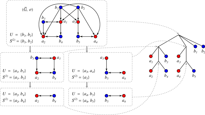
Figure 2: Illustration of Alg. 1 with input $(\mathaccent 382{G},\sigma)$ (uppermost box). The boxes indicate the five recursion steps that are necessary to decompose $(\mathaccent 382{G},\sigma)$, and correspond to the five inner vertices of the LRT shown on the right. Note that, in the recursion step on $(\mathaccent 382{G}[\{a_{3},a_{4},b_{5}\}],\sigma_{|.})$, we have $U\neq S^{(2)}$.

Lemma 10.

Let $(\mathaccent 382{G},\sigma)$ be a connected 2-BMG. Then Alg. 1 returns the least resolved tree for $(\mathaccent 382{G},\sigma)$.

Proof.

Let $(T,\sigma)$ be the (unique) least resolved tree of $(\mathaccent 382{G},\sigma)$ with root $\rho$. The latter is supplied to Alg. 1 to initialize the tree. By Thm. 4, Lemma 9 and since $(\mathaccent 382{G},\sigma)$ is connected, the set of support leaves $S_{\rho}=S^{(2)}=S^{(1)}\neq\emptyset$ for the root $\rho$ is correctly identified in the top-level recursion of Alg. 1 (Line 1-1) and attached to the root $\rho$ (Line 1-1). According to Cor. 3, one can now proceed to recursively construct the LRTs for the connected components of $(\mathaccent 382{G}-S_{\rho},\sigma_{|.})$, which is done in Line 1-1. By Lemma 7, these connected components $(\mathaccent 382{G}_{v},\sigma_{|.})$ are exactly the BMGs $\mathaccent 382{G}(T(v),\sigma_{|.})$ with $v\in\operatorname{child}_{T}(\rho)\setminus\{S_{\rho}\}$ (Line 1). In particular, therefore, we have $V(\mathaccent 382{G}_{v})=L(T(v))$. Since $v\notin S_{\rho}$, i.e., $v$ is an inner vertex, Cor. 1 and $v\prec_{T}\rho$ imply $|\sigma(L(T(v)))|>1$. Hence, in particular, the condition $|V(\mathaccent 382{G}_{v})|>1$ (cf. Line 1) to proceed recursively is satisfied for each connected component. ∎

Theorem 5.

Given a connected properly 2-colored digraph $(\mathaccent 382{G},\sigma)$ as input, Alg. 1 returns a tree $T$ if and only if $(\mathaccent 382{G},\sigma)$ is a 2-colored BMG. In particular, $T$ is the unique least resolved tree for $(\mathaccent 382{G},\sigma)$.

Proof.

By Lemma 10, Alg. 1 returns the unique least resolved tree $T$ if $(\mathaccent 382{G},\sigma)$ is a connected 2-colored BMG. To prove the converse, suppose that Alg. 1 returns a tree $T$ given the connected properly 2-colored digraph $(\mathaccent 382{G},\sigma)$ as input. We will show that $(\mathaccent 382{G},\sigma)=\mathaccent 382{G}(T,\sigma)$, and thus $(\mathaccent 382{G},\sigma)$ is a BMG.

It is easy to see that $L(T)=V(\mathaccent 382{G})$ must hold since, in each step of Alg. 1 every vertex is either attached to some inner vertex or passed down to a deeper-level recursion as part of some connected component. Therefore, every vertex of $\mathaccent 382{G}$ eventually appears in the output. Thus $\sigma(L(T))=\sigma(V(\mathaccent 382{G}))$ and $|\sigma(L(T))|=|\sigma(V(\mathaccent 382{G}))|=2$. It remains to show $E(\mathaccent 382{G})=E(\mathaccent 382{G}(T,\sigma))$.

Note first that neither $(\mathaccent 382{G},\sigma)$ nor $\mathaccent 382{G}(T,\sigma)$ contain arcs between vertices of the same color. Moreover, since Alg. 1 eventually returns a tree, we have $S^{(1)}=S^{(2)}\neq\emptyset$ in every recursion step. Throughout the remainder of the proof, we will write $S^{(1)}_{i}$ and $S^{(2)}_{i}$ for the sets $S^{(1)}$ and $S^{(2)}$ of the $i^{th}$ recursion step. Likewise, in every step, each connected component $(\mathaccent 382{G}_{v},\sigma_{|.})$ computed in Line 1 must contain at least two vertices (cf. Line 1), and thus $|\sigma(V(\mathaccent 382{G}_{v}))|=2$ because $(\mathaccent 382{G},\sigma)$ is properly 2-colored.

First, let $S$ be the support set of $\mathaccent 382{G}(T,\sigma)$ and $x\in S$ be arbitrary. Note that the support set is computed in the first iteration step of the algorithm as $S=S^{(2)}_{1}$, hence $S=S^{(2)}_{1}\neq\emptyset$. By construction of $T$, $x$ is attached as a leaf to $\rho$, i.e. $\operatorname{lca}_{T}(x,y)=\rho$. Consequently, $(x,y)$ is an arc in $\mathaccent 382{G}(T,\sigma)$ for all $y\in V(\mathaccent 382{G})$ with $\sigma(y)\neq\sigma(x)$. By construction of $S$ in Alg. 1, we have $x\in S\subseteq U$, i.e. $x$ is an umbrella vertex in $(\mathaccent 382{G},\sigma)$ and has out-arcs to every vertex $y\in V(\mathaccent 382{G})$ with $\sigma(y)\neq\sigma(x)$. Hence, all arcs of the form $(x,y)$ with $x\in S$ and $\sigma(x)\neq\sigma(y)$ exist both in $(\mathaccent 382{G},\sigma)$ and in $\mathaccent 382{G}(T,\sigma)$. The latter property is in particular satisfied for all vertices in $S$ and hence, all arcs between differently colored elements in $S$ exist both in $(\mathaccent 382{G},\sigma)$ and in $\mathaccent 382{G}(T,\sigma)$. Now consider an arbitrary vertex $y\in V(\mathaccent 382{G})\setminus S$. Clearly, all in-neighbors in $(\mathaccent 382{G},\sigma)$ of the elements in $S=S^{(2)}_{1}$ must be contained in $S$, as a consequence of the condition $S^{(1)}_{1}=S^{(2)}_{1}$ (cf. Line 1) and the construction of $S^{(1)}_{1}$ and $S^{(2)}_{1}$. Hence, $y\notin S$ and $x\in S$ implies that $(y,x)$ is not an arc in $(\mathaccent 382{G},\sigma)$. Moreover, $y\notin S$ also implies that $y$ is part of some connected component $(\mathaccent 382{G}_{v},\sigma_{|.})$ of $(\mathaccent 382{G}-S,\sigma_{|.})$. Therefore, and because Alg. 1 returns $T$, we must have $y\in V(\mathaccent 382{G}_{v})=L(T(v))$ for some inner vertex $v\in\operatorname{child}_{T}(\rho)$. As argued above, $(\mathaccent 382{G}_{v},\sigma_{|.})$ and thus also the subtree $T(v)$ contain both colors. Together with Obs. 3 and $x\notin L(T(v))$, this implies that $\mathaccent 382{G}(T,\sigma)$ does not contain the arc $(y,x)$. By the same arguments, there is no arc $(y,x^{\prime})$ in $\mathaccent 382{G}(T,\sigma)$ such that the vertex $x^{\prime}$ is contained in a different connected component $(\mathaccent 382{G}_{v^{\prime}},\sigma_{|.})\neq(\mathaccent 382{G}_{v},\sigma_{|.})$ of $(\mathaccent 382{G}-S,\sigma_{|.})$ than $y$. Since $x\in S$ and $y\notin S$ were chosen arbitrarily, we conclude that (i) any arc incident to some vertex in $S$ exists in $(\mathaccent 382{G},\sigma)$ if and only if it exists in $\mathaccent 382{G}(T,\sigma)$, and (ii) $\mathaccent 382{G}(T,\sigma)$ contains no arcs between distinct connected components of $(\mathaccent 382{G}-S,\sigma_{|.})$. Hence, it remains to consider the arcs within a connected component $(\mathaccent 382{G}_{v},\sigma_{|.})$ of $(\mathaccent 382{G}-S,\sigma_{|.})$.

Alg. 1 recurses on each such connected component $(\mathaccent 382{G}_{v},\sigma_{|.})$ using a newly created vertex $v\in\operatorname{child}_{T}(\rho)$ to initialize the tree $T(v)$. By Lemma 3, it clearly holds that, for any $x,y\in L(T(v))=V(\mathaccent 382{G}_{v})$, $(x,y)$ is an arc in $\mathaccent 382{G}(T,\sigma)$ if and only it is an arc in $\mathaccent 382{G}(T(v),\sigma)$. Thus, it suffices to consider only the subtree $T(v)$. Now, we can apply the same arguments as in the previous recursion step to conclude that all arcs incident to the support set $S^{(2)}_{2}$ constructed in the current recursion step are the same in $(\mathaccent 382{G},\sigma)$ and $\mathaccent 382{G}(T,\sigma)$ and that neither $(\mathaccent 382{G},\sigma)$ nor $\mathaccent 382{G}(T,\sigma)$ contain arcs between distinct connected components of $(\mathaccent 382{G}_{v}-S^{(2)}_{2},\sigma_{|.})$. Hence, it suffices to consider the connected components of $(\mathaccent 382{G}_{v}-S^{(2)}_{2},\sigma_{|.})$. Repeated application of this argumentation results in a chain of connected components that are contained in each other. Since Alg. 1 finally returns a tree, this chain is finite, say with a last element $(\mathaccent 382{G}_{w}-S^{(2)}_{k},\sigma_{|.})$, and thus $S^{(2)}_{k}=V(\mathaccent 382{G}_{w})$. In particular, therefore, every vertex in $V(\mathaccent 382{G})$ is contained in the support set of some recursion step.

In summary, we have shown that $\mathaccent 382{G}(T,\sigma)=(\mathaccent 382{G},\sigma)$. Hence, $(\mathaccent 382{G},\sigma)$ is a connected 2-BMG and, by Lemma 10, $T$ is the unique least resolved tree of $(\mathaccent 382{G},\sigma)$. ∎

The construction in Lines 1-1 in Alg. 1 naturally produces two cases, $U=S^{(1)}=S^{(2)}$ and $S^{(2)}\subseteq S^{(1)}\subsetneq U$. The following result shows that the latter case implies that the corresponding interior node in the LRT has only a single non-leaf descendant:

Lemma 11.

Let $(\mathaccent 382{G},\sigma)$ be a 2-BMG and $S_{\rho}$ the support leaves of the root $\rho$ of its LRT $(T,\sigma)$. If $W\coloneqq U(\mathaccent 382{G},\sigma)\setminus S_{\rho}\neq\emptyset$, then the following statements are true:

1. $S_{\rho}\neq\emptyset$, $\mathaccent 382{G}$ is connected, and $\mathaccent 382{G}-S_{\rho}$ is connected.

2. All vertices in $U(\mathaccent 382{G},\sigma)=S_{\rho}\mathbin{\mathchoice{\leavevmode\vtop{\halign{\hfil$\m@th\displaystyle#$\hfil\cr\cup\cr\cdot\crcr}}}{\leavevmode\vtop{\halign{\hfil$\m@th\textstyle#$\hfil\cr\cup\cr\cdot\crcr}}}{\leavevmode\vtop{\halign{\hfil$\m@th\scriptstyle#$\hfil\cr\cup\cr\cdot\crcr}}}{\leavevmode\vtop{\halign{\hfil$\m@th\scriptscriptstyle#$\hfil\cr\cup\cr\cdot\crcr}}}}W$ have the same color,

3. The set of support leaves $S_{v}$ of the unique inner vertex child $v$ of $\rho$ contains vertices of both colors, and

4. $W\subsetneq S_{v}$.

Proof.

First recall that, by Thm. 4 and the definition of the support set $S$ of $(\mathaccent 382{G},\sigma)$, we have $S_{\rho}=S\subseteq U(\mathaccent 382{G},\sigma)$, and thus $U(\mathaccent 382{G},\sigma)=S_{\rho}\mathbin{\mathchoice{\leavevmode\vtop{\halign{\hfil$\m@th\displaystyle#$\hfil\cr\cup\cr\cdot\crcr}}}{\leavevmode\vtop{\halign{\hfil$\m@th\textstyle#$\hfil\cr\cup\cr\cdot\crcr}}}{\leavevmode\vtop{\halign{\hfil$\m@th\scriptstyle#$\hfil\cr\cup\cr\cdot\crcr}}}{\leavevmode\vtop{\halign{\hfil$\m@th\scriptscriptstyle#$\hfil\cr\cup\cr\cdot\crcr}}}}W$. Moreover, by Lemma 7, the connected components of $(\mathaccent 382{G}-S_{\rho},\sigma_{|.})$ are exactly the BMGs $\mathaccent 382{G}(T(v),\sigma_{|.})$ with $v\in\operatorname{child}(\rho)\setminus S_{\rho}$. The vertices $v\in\operatorname{child}(\rho)\setminus S_{\rho}$ are all inner vertices of $T$ since, by definition, the support leaves $S_{\rho}$ are exactly the children of $\rho$ that are leaves. Together with the contraposition of Lemma 5 this implies that $T(v)$ contains both colors.

Statement 1: Let $x\in W$, which exists due to the assumption $W\coloneqq U(\mathaccent 382{G},\sigma)\setminus S_{\rho}\neq\emptyset$. Since $x\notin S_{\rho}$, it must be part of some connected component of $(\mathaccent 382{G}-S_{\rho},\sigma_{|.})$, say $\mathaccent 382{G}(T(v),\sigma_{|.})$ for some $v\in\operatorname{child}_{T}(\rho)\setminus S_{\rho}$. Now assume, for contradiction, that $\mathaccent 382{G}-S_{\rho}$ consists of more than one connected component. By Lemmas 7 and 5, there is a vertex $v^{\prime}\in\operatorname{child}_{T}(\rho)\setminus S_{\rho}$ such that $v\neq v^{\prime}$ and both subtrees $T(v)$ and $T(v^{\prime})$ contain both colors. Hence, there are distinct $y\in L(T(v))$ and $y^{\prime}\in L(T(v^{\prime}))$ with $\sigma(y)=\sigma(y^{\prime})\neq\sigma(x)$. Together with $x\in L(T(v))$, we therefore have $\operatorname{lca}_{T}(x,y)\preceq_{T}v\prec_{T}\rho=\operatorname{lca}_{T}(x,y^{\prime})$, which implies $(x,y^{\prime})\notin E(\mathaccent 382{G})$. However, $x\in W\subseteq U(\mathaccent 382{G},\sigma)$ and $\sigma(y^{\prime})\neq\sigma(x)$ imply $(x,y^{\prime})\in E(\mathaccent 382{G})$; a contradiction. Hence, we conclude that $\mathaccent 382{G}-S_{\rho}$ has exactly one connected component, and thus $\rho$ has a single inner vertex child $v$. Since $T$ is phylogenetic, the latter implies that $\rho$ must be incident to at least one leaf, i.e. $S_{\rho}\neq\emptyset$. Together with Thm. 4 this in turn implies that $\mathaccent 382{G}$ is connected. In summary, Statement 1 is true.

Statement 2: Let $x\in W$ as in the proof of Statement 1. By arguments analogous to those used for Statement 1, we conclude that $\sigma(x)=\sigma(y)$ for every $y\in S_{\rho}$, since otherwise we would obtain $(x,y)\notin E(\mathaccent 382{G})$, and thus a contradiction to $x\in U(\mathaccent 382{G},\sigma)$. Since $x\in W$ was chosen arbitrarily and $S_{\rho}$ is non-empty, we immediately obtain that all vertices in $U(\mathaccent 382{G},\sigma)=S_{\rho}\mathbin{\mathchoice{\leavevmode\vtop{\halign{\hfil$\m@th\displaystyle#$\hfil\cr\cup\cr\cdot\crcr}}}{\leavevmode\vtop{\halign{\hfil$\m@th\textstyle#$\hfil\cr\cup\cr\cdot\crcr}}}{\leavevmode\vtop{\halign{\hfil$\m@th\scriptstyle#$\hfil\cr\cup\cr\cdot\crcr}}}{\leavevmode\vtop{\halign{\hfil$\m@th\scriptscriptstyle#$\hfil\cr\cup\cr\cdot\crcr}}}}W$ have the same color, i.e., Statement 2 is true.

Statement 3: Now consider the single inner vertex child $v$ of $\rho$, and its set of support leaves $S_{v}$, which must be non-empty by Lemma 6. Note that $W$ must be entirely contained in $L(T(v))$ and recall that all vertices in $S_{\rho}\mathbin{\mathchoice{\leavevmode\vtop{\halign{\hfil$\m@th\displaystyle#$\hfil\cr\cup\cr\cdot\crcr}}}{\leavevmode\vtop{\halign{\hfil$\m@th\textstyle#$\hfil\cr\cup\cr\cdot\crcr}}}{\leavevmode\vtop{\halign{\hfil$\m@th\scriptstyle#$\hfil\cr\cup\cr\cdot\crcr}}}{\leavevmode\vtop{\halign{\hfil$\m@th\scriptscriptstyle#$\hfil\cr\cup\cr\cdot\crcr}}}}W$ are of the same color (cf. Statement 2). First suppose, for contradiction, that $S_{v}$ only contains vertices of the opposite color as the vertices in $S_{\rho}\mathbin{\mathchoice{\leavevmode\vtop{\halign{\hfil$\m@th\displaystyle#$\hfil\cr\cup\cr\cdot\crcr}}}{\leavevmode\vtop{\halign{\hfil$\m@th\textstyle#$\hfil\cr\cup\cr\cdot\crcr}}}{\leavevmode\vtop{\halign{\hfil$\m@th\scriptstyle#$\hfil\cr\cup\cr\cdot\crcr}}}{\leavevmode\vtop{\halign{\hfil$\m@th\scriptscriptstyle#$\hfil\cr\cup\cr\cdot\crcr}}}}W$. This immediately implies $S_{v}\cap W=\emptyset$, thus every vertex $x\in W$ must be located in a subtree $T(w)$ of some inner vertex child $w$ of $v$. Again by contraposition of Lemma 5, every such $T(w)$ contains both colors. However, this contradicts $(x,y)\in E(\mathaccent 382{G})$ for every $y\in S_{v}$, which must hold as a consequence of $x\in W\subset U(\mathaccent 382{G},\sigma)$ and $\sigma(y)\neq\sigma(x)$. Next suppose, for contradiction, that $S_{v}$ only contains vertices of the same color as the vertices in $S_{\rho}\mathbin{\mathchoice{\leavevmode\vtop{\halign{\hfil$\m@th\displaystyle#$\hfil\cr\cup\cr\cdot\crcr}}}{\leavevmode\vtop{\halign{\hfil$\m@th\textstyle#$\hfil\cr\cup\cr\cdot\crcr}}}{\leavevmode\vtop{\halign{\hfil$\m@th\scriptstyle#$\hfil\cr\cup\cr\cdot\crcr}}}{\leavevmode\vtop{\halign{\hfil$\m@th\scriptscriptstyle#$\hfil\cr\cup\cr\cdot\crcr}}}}W$. In this case, we obtain that the edge $\rho v$ is redundant w.r.t. $(\mathaccent 382{G},\sigma)$. To see this, consider an arc $(x,y)\in E(\mathaccent 382{G})$ such that $\operatorname{lca}_{T}(x,y)=v$. Clearly, $x$ must be directly incident to $v$, since otherwise the subtree below $v$ to which $x$ belongs would contain both colors, and thus contradict $(x,y)\in E(\mathaccent 382{G})$. In other words, every such vertex $x$ is a support leaf of $v$, thus $\sigma(x)=\sigma(S_{v})=\sigma(S_{\rho})$ and $\sigma(y)\neq\sigma(S_{\rho})$. In particular, there exists no arc $(x,y)\in E(\mathaccent 382{G})$ such that $\operatorname{lca}_{T}(x,y)=v$ and $\sigma(y)\in\sigma(L(T)\setminus L(T(v)))=\sigma(S_{\rho})$ and therefore, by Lemma 1, the inner edge $\rho v$ is redundant. However, this contradicts the fact that $T$ is least resolved. In summary, only the case in which $S_{v}\neq\emptyset$ contains vertices of both colors is possible, and thus Statement 3 is true.

Statement 4: First, recall from the proof of Statement 3 that $W\subseteq L(T(v))$ for the single inner vertex child $v$ of $\rho$. In order to see that $W\subseteq S_{v}$, assume for contradiction that this is not the case. By similar arguments as used for showing Statement 3, this implies that some $x\in W$ lies in a 2-colored subtree $T(w)$ for some $w\in\operatorname{child}_{T}(v)\setminus S_{v}$. Together with the above established fact that $S_{v}$ contains both colors, this contradicts $x\in U(\mathaccent 382{G},\sigma)$. Finally, $W\neq S_{v}$ is a consequence of the fact that $S_{v}$ contains both colors (Statement 3) but $W\subseteq S_{\rho}\mathbin{\mathchoice{\leavevmode\vtop{\halign{\hfil$\m@th\displaystyle#$\hfil\cr\cup\cr\cdot\crcr}}}{\leavevmode\vtop{\halign{\hfil$\m@th\textstyle#$\hfil\cr\cup\cr\cdot\crcr}}}{\leavevmode\vtop{\halign{\hfil$\m@th\scriptstyle#$\hfil\cr\cup\cr\cdot\crcr}}}{\leavevmode\vtop{\halign{\hfil$\m@th\scriptscriptstyle#$\hfil\cr\cup\cr\cdot\crcr}}}}W$ contains only one color (Statement 2). ∎

Figure 3: Illustration of Lemma 11. (A) The (local) situation if $W=U\setminus S_{\rho}\neq\emptyset$ as implied by Lemma 11. In particular, $\rho$ only as a single inner vertex child $v$, all vertices in $U=S_{\rho}\mathbin{\mathchoice{\leavevmode\vtop{\halign{\hfil$\m@th\displaystyle#$\hfil\cr\cup\cr\cdot\crcr}}}{\leavevmode\vtop{\halign{\hfil$\m@th\textstyle#$\hfil\cr\cup\cr\cdot\crcr}}}{\leavevmode\vtop{\halign{\hfil$\m@th\scriptstyle#$\hfil\cr\cup\cr\cdot\crcr}}}{\leavevmode\vtop{\halign{\hfil$\m@th\scriptscriptstyle#$\hfil\cr\cup\cr\cdot\crcr}}}}W$ have the same color, $S_{v}$ contains vertices of both colors, and $W\subsetneq S_{v}$. (B) There cannot be a second inner vertex child $v^{\prime}$, since then none of the vertices except those in $S_{\rho}$ can be umbrella vertices, e.g. $(a,b)$ is not an arc in the graph explained by the tree in (B). Hence, this situation is not possible for $W\neq\emptyset$. (C) If $S_{v}$ does not contain vertices of both colors, then the edge $\rho v$ is redundant in the tree, contradicting that $(T,\sigma)$ in Lemma 11 is the LRT.

We now use this result to consider the performance of Alg. 1.

Lemma 12.

Alg. 1 can be implemented to run in $O(|E|\log^{2}|V|)$ time for a connected input graph.

Proof.

Since $\mathaccent 382{G}$ is connected by assumption, we have $|V|\in O(|E|)$. Starting from $(\mathaccent 382{G},\sigma)$, the list of out-degrees can be constructed in $O(|E|)$. The initial umbrella set $U$ is then obtained by listing the vertices with maximal out-degree in the color class. The initial set $S^{(1)}$ is constructed by checking, for each $u\in U$, the in-neighbors of $u$ for membership in $U$ in $O(|V|+|E|)$ operations. Then $S^{(2)}$ is obtained in the same manner from $S^{(1)}$, requiring $O(|V|+|E|)$ operations. The initial umbrella set $U$ and the sets $S^{(1)}$ and $S^{(2)}$ thus can be constructed in linear time. In each recursive call of Build2ColLRT, at least one leaf is split off, hence the recursion depth is $|V|-1$ in the worst case. Since the support vertices removed in each step have all of their in-neighbors in $U$, their removal does not affect the out-neighborhood for any $x\in V(\mathaccent 382{G}-U)\subseteq V(\mathaccent 382{G}-S^{(2)})$, and hence, $\operatorname{outdeg}(x)$ does not require updates. The in-neighborhoods $N^{-}(x)$ can be updated by removing the arcs between $\mathaccent 382{G}-S^{(2)}$ and $S^{(2)}$ as a consequence of Lemma 7 and Thm. 4. Since every arc appears exactly once in the removal, the total effort for these updates is $O(|E|)$.

We continue by showing that every vertex needs to be considered as an umbrella vertex at most twice, and that the total effort of constructing all sets $S^{(1)}$ and $S^{(2)}$ is $O(|E|)$, given that the umbrella vertices $U$ can be obtained efficiently, which we discuss afterwards. To this end, we distinguish, for each of the single recursion steps, two cases: $S^{(1)}=U$ and $S^{(1)}\subsetneq U$. First if $S^{(1)}=U$, and thus also $S^{(2)}=S^{(1)}=U$, we consider each in-arc of $x\in U$. Since these vertices and their corresponding arcs are removed when constructing $\mathaccent 382{G}-S^{(2)}$, they are not considered again in a deeper recursion step. In the second case, we have $S^{(1)}\subsetneq U$, which together with $S^{(2)}=S^{(1)}$ implies $W\coloneqq U\setminus S^{(2)}\neq\emptyset$, and only the vertices in $U\setminus W$ are removed. However, Lemma 11 guarantees that, for a 2-BMG as input graph, the vertices in $W$ appear as support leaves in the next step and thus appear in the update of $U$, $S^{(1)}$, and $S^{(2)}$ no more than a second time. In order to use the properties in Lemma 11 for the general case (i.e. $(\mathaccent 382{G},\sigma)$ is not necessarily a BMG), we can, whenever $W\neq\emptyset$, (i) check that $\mathaccent 382{G}-S^{(2)}$ only has a single connected component $\mathaccent 382{G}_{v}$, and (ii) pass down the set $W$ to the recursion step on $\mathaccent 382{G}_{v}$ in which the condition $W\subsetneq S^{(2)}$ is checked. If any of these checks fails, we can exit false. This way, we ensure that every vertex appears at most two times as an umbrella vertex in the general case. To construct $S^{(1)}$ from $U$, we have to scan the in-neighborhood $N^{-}(x)$ of each vertex $x\in U$ and check whether $N^{-}(x)\subset U$. We repeat this step to construct $S^{(2)}$ from $S^{(1)}$. Membership in $U$ and $S^{(1)}$, resp., can be checked in constant time (e.g. by marking the vertices in the current set $U$). Since we have to consider each vertex, and hence, each in-neighborhood at most twice, all sets $S^{(1)}$ and $S^{(2)}$ can be obtained with a total effort of $O(|E|)$.

It remains to show that the input graph can be decomposed efficiently in such a way that the connectivity information is maintained and the candidates for umbrella vertices in each component are updated. The connected components $\mathaccent 382{G}_{v}$ can be obtained by using the dynamic data structure described in [6], often called HDT data structure. It maintains a maximal spanning forest representing the underlying undirected graph with edge set $\widetilde{E}=\{xy\mid(x,y)\in E\textrm{ or }(y,x)\in E\}$, and allows deletion of all $|\widetilde{E}|\in O(|E|)$ edges with amortized cost $O(\log^{2}|V|)$ per edge deletion. The explicit traversal of the connected components to compute $U$ can be avoided as follows: Since $\operatorname{outdeg}(x)$ does not require updates, we can maintain a doubly-linked list of vertices $x$ for each color $i\in\{1,2\}$, and each value of $\operatorname{outdeg}(x)$ where $\sigma(x)=i$. In order to be able to access the highest value of the out-degrees, we maintain these values together with pointer to the respective doubly-linked list in balanced binary search trees (BST), one for each color and each connected component. The BSTs for the two colors are computed first for $(\mathaccent 382{G},\sigma)$ in $O(|V|\log(|V|))$ time and afterwards updated to fit with the out-degree of the currently considered component $\mathaccent 382{G}_{v}$. To update these lists and BSTs for $\mathaccent 382{G}_{v}$, observe first that $\mathaccent 382{G}_{v}$ can be obtained from $G$ by stepwise deletion of single arcs, i.e. edges in the HDT data structure representing the underlying undirected versions. We update, resp., construct the pair of BSTs (one for each color) for each connected component as follows: Since a single arc deletion splits a connected component $\mathaccent 382{G}^{\prime}$ into at most two connected components $\mathaccent 382{G}_{1}$, and $\mathaccent 382{G}_{2}$, we can apply the well-known technique of traversing the smaller component [14]. The size of each connected component can be queried in $O(1)$ time in the HDT data structure. Suppose w.l.o.g. that $|V(\mathaccent 382{G}_{1})|\leq|V(\mathaccent 382{G}_{2})|$. We construct a new pair of BSTs for $\mathaccent 382{G}_{1}$, and delete the vertices $V(\mathaccent 382{G}_{1})$ and the respective degrees from the two original BSTs for $\mathaccent 382{G}$, which then become the BSTs for $\mathaccent 382{G}_{2}$. More precisely, we delete each vertex $x\in V(\mathaccent 382{G}_{1})$ in the respective list corresponding to $\operatorname{outdeg}(x)$, and if the length of this list drops to zero, we also remove the corresponding out-degree in the BST. Likewise, we insert the out-degree of $x$ and an empty doubly-linked list into the newly-created BST for $\mathaccent 382{G}_{1}$, if it is not yet present, and append $x$ to this list. Note that the number of out-degree deletions and insertions does not exceed $|V(\mathaccent 382{G}_{1})|$. Due to the technique of traversing the smaller component, every vertex is deleted and inserted at most $\lfloor\log|V|\rfloor$ times. Therefore, we obtain an overall complexity of $O(|V|\log^{2}|V|)$ for the maintenance of the BSTs where the additional log-factor originates from rebalancing the BSTs whenever necessary.

In each recursion step, the set $U$ can now be obtained by listing (at most) the vertices with the maximal out-degree for each of the two colors. Finding the two out-degrees and corresponding lists in the BSTs requires $O(\log|V|)$ in each step, and thus $O(|V|\log|V|)$ in total. In order to determine whether these candidates $x$ are actually umbrella vertices, we have to check whether $\operatorname{outdeg}(x)=|V(G_{v})|-|V(G_{v})[\sigma(x)]|$. The HDT data structure allows constant-time query of the size of a given connected component, since this information gets updated during the maintenance of the spanning forest. By the same means, we can keep track of the number of vertices of a specific color in each connected components. Note that we only need to do this for one color $r$ since $|V(G_{v})[s]|=|V(G_{v})|-|V(G_{v})[r]|$. This does not increase the overall effort for maintaining the data structure since it happens alongside the update of $|V(G_{v})|$.

In summary, the total effort is dominated by maintaining the connectedness information while deleting $O(|E|)$ arcs, i.e., $O(|E|\log^{2}|V|)$ time. ∎

As a direct consequence of Thm. 4 the LRT of a disconnected graph $\mathaccent 382{G}$ is obtained by connecting the roots of the LRTs $T_{v}$ of the connected components $G_{v}$ to an additional root vertex, see also [5, Cor. 4]. Lemma 12 thus implies

Theorem 6.

The LRT of a 2-BMG can be computed in $O(|V|+|E|\log^{2}|V|)$.

Proof.

The connected components $G_{i}=(V_{i},E_{i})$ of $G=(V,E)$ can be enumerated in $O(|V|+|E|)$ operations, e.g. using a breadth-first search on the underlying undirected graph. By Lemma 12, $O(|E_{i}|\log^{2}|V_{i}|)\leq O(|E_{i}|\log^{2}|V|)$ operations are required for each $G_{i}$. Hence, the total effort is $O(|V|+|E|+\log^{2}|V|\sum_{i}|E_{i}|)=O(|V|+|E|\log^{2}|V|)$. ∎

In order to illustrate the improved complexity for the construction of LRTs of 2-BMGs, we implemented both the well-known triple-based approach, i.e., the application of BUILD [2] with the informative triples defined in Eq. (1) as input, and the new approach of Alg. 1. As input, we used 2-BMGs that where randomly generated as follows: First, we simulate random trees $T$ recursively, starting from a single vertex, by attaching to a randomly chosen vertex $v$ either a single leaf if $v$ is an inner vertex of $T$ or a pair of leaves if $v$ was a leaf. The construction stops when the desired number of leaves is reached. Note that the resulting tree is phylogenetic by construction. Each leaf is then colored by selecting at random one of the two colors. Finally, we compute the 2-BMG $\mathaccent 382{G}(T,\sigma)$ from each of the simulated leaf-colored trees $(T,\sigma)$.

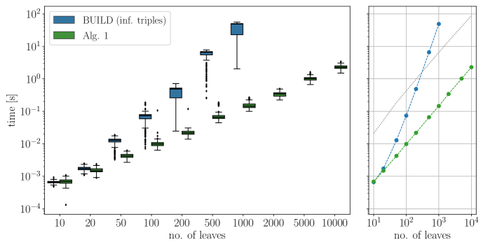
Figure 4: Running time comparison of the general approach for constructing an LRT using BUILD (blue) vs. Alg. 1 (green). For each number of leaves, 200 2-BMGs where generated as described in the text. In the left panel, the median values are shown with logarithmic axes. The additional dotted line indicates the median values of the size of the simulated BMGs, i.e. the number of arcs, scaled by a factor $10^{-3}$. We did not compute the LRTs with the first method for instances with more than 1000 leaves because of the excessive computational cost.

Both methods for the LRT computation were implemented in Python. Moreover, we note that we did not implement the sophisticated dynamic data structures used in the proof of Lemma 12, but a rather naïve implementation of Alg. 1. Nevertheless, Fig. 4 shows a remarkable improvement of the running time when compared to the general $O(|V|\,|E|\log^{2}|V|)$ approach for $\ell$-BMGs detailed in [5]. Empirically, we observe that the running time of Alg. 1 indeed scales nearly linearly with the number of edges.

6 Binary-explainable 2-BMGs

Binary phylogenetic trees are of particular interest in practical applications. Not every 2-BMG can be explained by a binary tree. The subclass of binary-explainable ($\ell$-)BMG are characterized among all BMGs by the absence of single forbidden subgraph called hourglass [10, 11], illustrated in Fig. 5. In this section we briefly describe a modification of Alg. 1 that allows the efficient recognition of binary-explainable 2-BMGs.

Definition 9.

An hourglass in a properly vertex-colored graph $(\mathaccent 382{G},\sigma)$, denoted by $[xy\mathrel{\text{\ooalign{$\searrow$\cr$\nearrow$}}}x^{\prime}y^{\prime}]$, is a subgraph $(\mathaccent 382{G}[Q],\sigma_{|Q})$ induced by a set of four pairwise distinct vertices $Q=\{x,x^{\prime},y,y^{\prime}\}\subseteq V(\mathaccent 382{G})$ such that (i) $\sigma(x)=\sigma(x^{\prime})\neq\sigma(y)=\sigma(y^{\prime})$, (ii) $(x,y),(y,x)$ and $(x^{\prime}y^{\prime}),(y^{\prime},x^{\prime})$ are bidirectional arcs in $\mathaccent 382{G}$, (iii) $(x,y^{\prime}),(y,x^{\prime})\in E(\mathaccent 382{G})$, and (iv) $(y^{\prime},x),(x^{\prime},y)\notin E(\mathaccent 382{G})$.

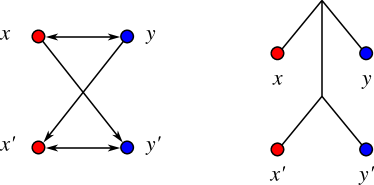
Figure 5: The tree on the r.h.s. explains the hourglass graph on the l.h.s.

A graph $(\mathaccent 382{G},\sigma)$ is called hourglass-free if it does not contain an hourglass as an induced subgraph. We summarize Lemma 31 and Prop. 8 in [11] as

Proposition 3.

For every BMG $(\mathaccent 382{G},\sigma)$, the following three statements are equivalent:

1. $(\mathaccent 382{G},\sigma)$ is binary-explainable.

2. $(\mathaccent 382{G},\sigma)$ is hourglass-free.

3. If $(T,\sigma)$ is a tree explaining $(\mathaccent 382{G},\sigma)$, then there is no vertex $u\in V^{0}(T)$ with three distinct children $v_{1}$, $v_{2}$, and $v_{3}$ and two distinct colors $r$ and $s$ satisfying

   1. $r\in\sigma(L(T(v_{1})))$, $r,s\in\sigma(L(T(v_{2})))$, and $s\in\sigma(L(T(v_{3})))$, and

   2. $s\notin\sigma(L(T(v_{1})))$, and $r\notin\sigma(L(T(v_{3})))$.

The following Lemma shows that the third condition in Prop. 3 can be translated to a much simpler statement in terms of the support leaves of its LRT.

Lemma 13.

A 2-BMG $(\mathaccent 382{G},\sigma)$ contains an induced hourglass if and only if its LRT $(T,\sigma)$ contains an inner vertex $u$ such that $S_{u}$ contains support vertices of both colors and $V(\mathaccent 382{G}(T(u))-S_{u})\neq\emptyset$.

Proof.

By Thm. 5, Alg. 1 returns the LRT $(T,\sigma)$ for $(\mathaccent 382{G},\sigma)$ if and only if $(\mathaccent 382{G},\sigma)$ is a 2-BMG. Hence, we assume in the following that the latter is satisfied. As a consequence of Prop. 3 and the fact that $(T,\sigma)$ explains $(\mathaccent 382{G},\sigma)$, we know that $(\mathaccent 382{G},\sigma)$ is binary-explainable if and only if there is no vertex $u\in V^{0}(T)$ with three distinct children $v_{1}$, $v_{2}$, and $v_{3}$ and two distinct colors $r$ and $s$ satisfying (a) $r\in\sigma(L(T(v_{1})))$, $r,s\in\sigma(L(T(v_{2})))$, and $s\in\sigma(L(T(v_{3})))$, and (b) $s\notin\sigma(L(T(v_{1})))$, and $r\notin\sigma(L(T(v_{3})))$.

First, suppose that $(\mathaccent 382{G},\sigma)$ contains an hourglass, i.e., by Prop. 3 there is a vertex $u\in V^{0}(T)$ with distinct children $v_{1}$, $v_{2}$, and $v_{3}$ and two distinct colors $r$ and $s$ satisfying (a) and (b). Since $(\mathaccent 382{G},\sigma)$ is 2-colored and $(T,\sigma)$ its LRT, Lemma 5 together with $s\notin\sigma(L(T(v_{1})))$ and $r\notin\sigma(L(T(v_{3})))$ implies that $v_{1}$ of color $r$ and $v_{2}$ of color $s$, respectively, are both leaves. In particular, therefore, we know that $v_{1},v_{2}\in S_{u}$ are support leaves. By Lemma 7 and since $\mathaccent 382{G}(T(u),\sigma_{|.})$ is also a BMG, the connected components of $(\mathaccent 382{G}(T(u))-S_{u},\sigma_{|.})=(\mathaccent 382{G}[L(T(u))]-S_{u},\sigma_{|.})$ (cf. Lemma 3) are exactly the BMGs $\mathaccent 382{G}(T(v),\sigma_{|.})$ with $v\in\operatorname{child}(u)\setminus S_{u}$. Together with the fact that $v_{2}\in V^{0}(T)$ as a consequence of $L(T(v_{2}))$ containing both colors $r$ and $s$, this implies that $(\mathaccent 382{G}(T(u))-S_{u},\sigma_{|.})$ is not the empty graph.

Conversely, suppose there a vertex $u\in V^{0}(T)$ such that $S_{u}$ contains support vertices $v_{1}$ and $v_{3}$ with distinct colors $\sigma(v_{1})\neq\sigma(v_{3})$ and $V(\mathaccent 382{G}(T(u))-S_{u})\neq\emptyset$, i.e., $u$ has a child $v_{2}\in\operatorname{child}(u)\setminus S_{u}$ that is not a support leaf and hence satisfies $v_{2}\in V^{0}(T)$. Lemma 5 implies that $L(T(v_{2}))$ contains both colors since $v_{2}\in V^{0}(T)$. Hence, the three children $v_{1}$, $v_{2}$, and $v_{3}$ of $u$ satisfy conditions (a) and (b) of Prop. 3(3), and thus $(\mathaccent 382{G},\sigma)$ contains an induced hourglass. ∎

Corollary 4.

It can be checked in $O(|V|+|E|\log^{2}|V|)$ whether or not a properly 2-colored graph $(\mathaccent 382{G},\sigma)$ is a binary-explainable BMG.

Proof.

Recall that there is a one-to-one correspondence between the recursion step in Alg. 1 and the inner vertices $u\in V^{0}(T)$. As argued in the proof of Lemma 12, every vertex appears at most twice in an umbrella set $U$. Therefore, it can be checked in $O(|V|)$ total time whether $S=S^{(2)}$ contains vertices of both colors. Since the vertex set of $\mathaccent 382{G}_{u}-S_{u}$ is maintained in the dynamic graph HDT data structure, it can be checked in constant time for each $u$ whether $\mathaccent 382{G}_{u}-S_{u}$ is non-empty. The additional effort to check the condition of Lemma 13 is therefore only $O(|V|)$. Hence, we still require a total effort of $O(|V|+|E|\log^{2}|V|)$ (cf. Thm. 6). ∎

Cor. 4 improves the complexity for the decision whether a 2-BMG is binary-explainable as compared to the $O(|V|^{3}\log^{2}|V|)$-time algorithm for (general) BMGs presented in [10].

7 Concluding Remarks

We have shown here that 2-BMGs have a recursive structure that is reflected in certain induced subgraphs that correspond to subtrees of the LRT. The leaves connected directly to the root of a given subtree play a special role as support vertices in the corresponding subgraph of the 2-BMG. Since the support vertices of the root can be identified efficiently in a given input graph, there is a recursive decomposition of $(\mathaccent 382{G},\sigma)$ that directly yields the LRT. With the help of a dynamic data structure to maintain connectedness information [6], this provides an $O(|V|+|E|\log^{2}|V|)$ algorithm to recognize both 2-BMGs and binary explainable 2-BMGs and to construct the corresponding LRT. This provides a considerable speed-up compared to the previously known $O(|V||E|\log^{2}|V|)$ and $O(|V|^{3})$ algorithms. Empirically, we observe a substantial speed-up even if simpler data structures are used to implement Alg. 1.

Both the theoretical insights and Alg. 1 itself have potential applications to the analysis of gene families in computational biology. Real-life data necessarily contain noise, and thus likely will deviate from perfect BMGs, naturally leading to graph editing problems for BMGs. Like many combinatorial problems in phylogenetics, these are NP-complete [12] and hence require approximation algorithms and heuristics. The support leaves introduced here provide an avenue to a new class of heuristics, conceptually distinct from approaches that attempt to extract consistent subsets of triples from $\mathscr{R}(\mathaccent 382{G},\sigma)$.

References

- [1] G. Abrams and J. K. Sklar. The graph menagerie: Abstract algebra and the mad veterinarian. Math. Mag., 83:168–179, 2010. doi:10.4169/002557010X494814.
- [2] A. Aho, Y. Sagiv, T. Szymanski, and J. Ullman. Inferring a tree from lowest common ancestors with an application to the optimization of relational expressions. SIAM J Comput, 10:405–421, 1981. doi:10.1137/0210030.
- [3] H. Cohn, R. Pemantle, and J. G. Propp. Generating a random sink-free orientation in quadratic time. Electr. J. Comb., 9:R10, 2002. doi:10.37236/1627.
- [4] S. Das, P. Ghosh, S. Ghosh, and S. Sen. Oriented bipartite graphs and the Goldbach graph. Technical Report math.CO/1611.10259v6, arXiv, 2020.
- [5] M. Geiß, E. Chávez, M. González Laffitte, A. López Sánchez, B. M. R. Stadler, D. I. Valdivia, M. Hellmuth, M. Hernández Rosales, and P. F. Stadler. Best match graphs. J. Math. Biol., 78:2015–2057, 2019. doi:10.1007/s00285-019-01332-9.
- [6] J. Holm, K. de Lichtenberg, and M. Thorup. Poly-logarithmic deterministic fully-dynamic algorithms for connectivity, minimum spanning tree, 2-edge, and biconnectivity. J. ACM, 48:723–760, 2001. doi:10.1145/502090.502095.
- [7] A. Korchmaros. Circles and paths in 2-colored best match graphs. Technical Report math.CO/2006.04100v1, arXiv, 2020.
- [8] A. Korchmaros. The structure of 2-colored best match graphs. Technical Report math.CO/2009.00447v2, arXiv, 2020.
- [9] D. Schaller, M. Geiß, E. Chávez, M. González Laffitte, A. López Sánchez, B. M. R. Stadler, D. I. Valdivia, M. Hellmuth, M. Hernández Rosales, and P. F. Stadler. Best match graphs (corrigendum). arxiv.org/1803.10989v4, 2020.
- [10] D. Schaller, M. Geiß, M. Hellmuth, and P. F. Stadler. Best match graphs with binary trees. 2020. submitted; arXiv 2011.00511.
- [11] D. Schaller, M. Geiß, P. F. Stadler, and M. Hellmuth. Complete characterization of incorrect orthology assignments in best match graphs. J. Math. Biol., 2021. accepted; arXiv: 2006.02249.
- [12] D. Schaller, P. F. Stadler, and M. Hellmuth. Complexity of modification problems for best match graphs. Theor. Comp. Sci., 2021. in revision; arxiv: 2006.16909.
- [13] C. Semple and M. Steel. Phylogenetics. Oxford University Press, Oxford UK, 2003.
- [14] Y. Shiloach and S. Even. An on-line edge-deletion problem. J. ACM, 28:1–4, 1981. doi:10.1145/322234.322235.