Robust Energy-Efficient Resource Management, SIC Ordering, and Beamforming Design for MC MISO-NOMA Enabled 6G

Abstract

This paper studies a novel approach for successive interference cancellation (SIC) ordering and beamforming in a multiple antennas non-orthogonal multiple access (NOMA) network with multi-carrier multi-user setup. To this end, we formulate a joint beamforming design, subcarrier allocation, user association, and SIC ordering algorithm to maximize the worst-case energy efficiency (EE). The formulated problem is a non-convex mixed integer non-linear programming (MINLP) which is generally difficult to solve. To handle it, we first adopt the linearizion technique as well as relaxing the integer variables, and then we employ the Dinkelbach algorithm to convert it into a more mathematically tractable form. The adopted non-convex optimization problem is transformed into an equivalent rank-constrained semidefinite programming (SDP) and is solved by SDP relaxation and exploiting sequential fractional programming. Furthermore, to strike a balance between complexity and performance, a low complex approach based on alternative optimization is adopted. Numerical results unveil that the proposed SIC ordering method outperforms the conventional existing works addressed in the literature.

I Introduction

I-A Motivations and State of the Art

In the recent decades, wireless communications have appealed to a growing number of customers, demanding high quality services, and ubiquitous connections. In order to fulfill these demands, the next generation of wireless networks, namely sixth-generation (6G), should be redesigned and exploit advanced technologies [1]. Regarding this, the network must be designed in such a way to dynamically change its architecture and the communications technologies. In such a flexible architecture, significant amount of signaling and computational resources are needed to optimally manage the network resources and enable to design the flexible resource sharing. Recently, various radio access network (RAN) architectures as distributed and centralized RAN (C-RAN) are developed to provide an efficient computational resource sharing and resource utilization [3]. To enable sustainable 6G networks, new emerging techniques such as new multiple access (MA) and multiple antennas systems (MAS) are needed to improve the network performance (e.g., energy efficiency (EE)) [5]. In this regard, non-orthogonal multiple access (NOMA) and multiple-input single-output (MISO) are promising approaches which can significantly improve EE and provide massive connectivity applications, i.e., Internet of Thing (IoT) compared to the orthogonal multiple access (OMA) and single antenna systems[6, 7, 8, 9]. In fact, improving the EE, fairness, and flexibility in resource allocation have turned to apply NOMA systems as the main trend in the beyond current wireless network. The authors in [9] present a basic principle of NOMA in which they state a systematic comparison among the different NOMA techniques from the viewpoint of the EE and receiver complexity. In particular, NOMA utilizes power domain (PD-NOMA) based networks for MA as well as successive interference cancellation (SIC) which removes the undesired multiuser interference[10]. In NOMA, SIC ordering is one of the key challenges and it is critical for the performance of data transmission to handle the NOMA interference [11, 12]. However, the SIC ordering problem has not been addressed well, and there are open problems that need to be addressed properly [11, 12]. In fact, in most of the works, SIC ordering is considered based on the channel gain which is not practical and optimal due to necessity of full channel state information (CSI) [25, 9, 14, 20, 18, 13, 17, 16]. Besides, there is uncertainty in the CSI that cannot be applicable for multiple antennas systems.
This paper proposes a worst-case SIC ordering, resource allocation policy, and beamforming design for multicarrier (MC) MISO-NOMA networks. We would like to see how much we can get performance gain in MAS for the SIC ordering as compared to OMA as well as traditional methods in which SIC ordering is based on the channel gains.

I-B Related Works

In NOMA, the efficient allocation of scarce resources and SIC ordering are turned into a challenging necessity for improving users’ satisfaction [11]. There are some attempts to find proper resource allocation strategies which improves the overall performance of such networks[15, 16, 14, 18, 13, 17]. For instance, the problem of power allocation and precoding design is proposed in [13] in which they employ single carrier multiple-input multiple-output (MIMO) NOMA systems. The authors in [14] propose an optimal resource allocation to maximize the system throughput for NOMA and full-duplex (FD) systems, respectively.  However, the base station (BS) is equipped with a single antenna which cannot fully exploit the degrees of freedom of the network. The works in [20, 22, 19, 32] consider beamforming design for MISO-NOMA systems to optimize the performance and cost of the system. In particular, the authors in [19] propose a robust beamforming design for MISO-NOMA system to maximize the minimum data rate. In [20], beamforming design and subcarrier allocation for maximizing the total data rate are proposed where optimal and sub-optimal solutions are provided. The beamforming design for maximizing the minimum EE and proportional fairness are developed in [22] to strike a balance between the EE of the system and the fairness between users. Most of the previous works considered the fixed SIC ordering, in which the order of decoding at each receiver is determined according to the channel gains [14, 20, 18, 13, 17, 16]. In SIC, the users are ordered and each user can remove the interference from users determined by the ordering scheme. Although most of the works on the SIC ordering sort the users based on their channels, this is not a practical scenario and can not be guaranteed as well. Also, it should be noted that sorting users for SIC based on the channel gains is neither optimal nor practical scheme at all, especially in MAS due to unavailability of the full CSI [20]. To circumvent this problem, SIC ordering should be based on the network, channel gain, and the available resource conditions. The authors in [21] address this problem for single antenna BS and perfect CSI scenario which is not practical and appropriate for future networks due to considering single-antenna BS and also having perfect CSI channel.

Besides, EE is an important metric for wireless networks, especially for enabling green communication. New communication technologies are proposed to improve the system EE. In particular, various techniques are proposed which aim to enhance the network throughput while consuming less energy without sacrificing the quality of service (QoS). At the same time, EE maximization problems are indispensable in NOMA systems, to strike a good throughput-power tradeoff and improve the system performance which is noticed as one of the key performance metrics in future wireless networks. However, there is a deficit of existing works on the literature considering the EE. For instance, in [23], EE maximization is studied to obtain an optimal power allocation based on the non-linear fractional programming method. Furthermore, in [24], a subchannel assignment and power allocation is investigated to maximize the EE in NOMA networks. However, in real scenarios assuming perfect CSI is not a valid assumption due to some issues like quantization and channel estimation errors as well as hardware limitations. In this regards the works in [19, 25, 27, 26] address the robust solution for imperfect CSI. In particular, in [19, 25, 27], robust designs for the MISO-NOMA systems are developed based on the bounded channel uncertainties. The joint user scheduling and power allocation are explored in [26] while considering imperfect CSI. User association in multi-cell NOMA systems is also challenging. Specifically, in addition to the NOMA interference caused by the co-channel interference, the interference between cells also needs to be taken into consideration [28, 29]. Nonetheless to the best of the authors knowledge, the problem of beamforming design and SIC ordering in a MC MISO-NOMA enabled C-RAN network while considering imperfect CSI has not been investigated yet. In [14, 21, 13, 18, 17, 16], the BS is equipped with single antenna while assuming perfect CSI. The works in [25, 27, 19] consider robust beamforming design while fixed SIC ordering. Furthermore, the authors in [28, 29] consider user association for the single antenna BS while SIC is based on the channel gains. In addition, in [21], the SIC ordering problem for single antenna BS and perfect CSI is considered. Consequently, user association policy and SIC ordering in a MISO-NOMA enabled C-RAN network with imperfect CSI are still open problems which have not been addressed yet.

I-C Contributions and Research Outcomes

In this paper, we aim to bridge the above mentioned knowledge gap. In particular, we propose a joint beamforming design, subcarrier allocation, user association, and SIC ordering algorithm which maximizes the EE of the network under imperfect CSI. To this end, we formulate the problem of beamforming design and SIC ordering to maximize the worst-case system EE. In our method, SIC ordering is considered as an optimization variable while in more existing works, SIC ordering is fixed and depends on the channel gains. The optimization problem is a non-convex mixed integer non-linear programming which is very difficult to solve. To handle it, we employ majorization minimization (MM), abstract Lagrangian method, semi-definite relaxation (SDR) method, and sequential fractional programming to handle the beamforming design and integer variables.

Our main contributions are summarized as follows:

• We propose a novel SIC ordering method for the downlink of a MC MISO NOMA. To this end, we formulate a novel optimization problem to maximize the EE by performing the subcarrier allocation, beamforming design, user association, and SIC ordering. In particular, we formulate a new problem to investigate how to order users to apply successful SIC based on the available resources. Also, we derive the worst-case SIC ordering condition as an optimization constraint and then tackle its non-convexity.

• We study the practical imperfect CSI in C-RAN networks. In doing so, we consider the worst-case EE to provide a robust resource allocation algorithm.

• We propose a solution based on rank-constrained semidefinite programming (SDP) relaxation and exploiting sequential fractional programming. In particular, we adopt MM approach and penalty factor to make it mathematically tractable and then we adopt Dinkelbach algorithm. Moreover, we provide a low complexity iterative algorithm in which the scheduling variable, i.e., user association and subcarrier assignment, is obtained through the matching algorithm.

• Numerical results reveal that the proposed worst-case EE maximization and SIC ordering algorithm can alleviate negative effect of imperfect of CSI, SIC, and limited power and spectrum resources on the network performance. Also, the results showcase the superiority of the proposed algorithm compared to the other conventional schemes.

The rest of this paper is organized as follows. The system model and problem formulation is discussed in Sec. II. The solution algorithm and complexity analysis are presented in Sec. III. Finally, the simulation analysis and conclusions are provided in Secs. IV and V, respectively.
Notations: Vector and matrix variables are indicated by bold lower-case and upper-case letters, respectively. $|.|$ indicate the absolute value, $\|.\|$ or $\|.\|_{2}$ denotes the Euclidean norm ($\textit{l}_{2}$ norm), and $\mathbb{A}^{\dagger}$ and $\mathbb{A}^{T}$ indicate the conjugate transpose and transpose of matrix $\mathbb{A}$, respectively. Also, $\text{Tr}[\mathbb{A}]$ denotes the trace of matrix $\mathbb{A}$ and $\mathbb{I}_{M}$ denotes the $M\times M$ identity matrix. $a^{*}$ denotes the optimal value of variable $a$. $\nabla_{\mathbb{x}}g$ indicate the gradient vector of function $g(\mathbb{x})$. $\mathcal{S}$ denotes the set $\{1,2,\dots,S\}$ and $|\mathcal{S}|=S$ is the cardinality of set $\mathcal{S}$. $\mathcal{S}\backslash\{s\}$ discards the element $s$ from the set $\mathcal{S}$. $\mathcal{C}^{M\times 1}$ denotes the set of $M$-by-$1$ dimensional complex vectors, and operation $\mathbb{E}\{.\}$ denotes the statistical expectation.

II System Model and Problem Formulation

II-A System Model Descriptions and Related Constraints

In this paper, we consider a downlink scenario for a C-RAN consisting of a set of $F$ active antenna units (AAUs) indexed by $f$, whose set is denoted by $\mathcal{F}=\{1,\dots,{F}\}$, where $f=1$ is a high power AAU, and a base band unit (BBU). Let $P_{\text{max}}^{f}$ be the transmit power budget of AAU $f$. Each AAU is equipped with $M$ antennas, uses a set $\mathcal{N}$ of $N$ shared subcarriers, is connected to the BBU with a limited bandwidth fronthaul/metro-edge link, and utilizes PD-NOMA to transmit data to single antenna end-users. In fact, we consider a MC MISO-NOMA communication network setup. We denote the set of all users as $\mathcal{K}=\{1,\dots,K\}$ which are randomly distributed with the uniform distribution inside the coverage/service area of the network [29, 32]. The considered system model is depicted in Fig. 1. Considering that user $2$ performs SIC on users $1$ and $3$ over subcarrier $2$, we have such output for SIC ordering variable which will be explained in Sec. II-A1, $\xi^{2}_{1,2}=1,\xi^{2}_{3,2}=1,\xi^{3}_{2,2}=0,$ and $\xi^{1}_{2,2}=0$. The definition of main notations are listed in Table I.

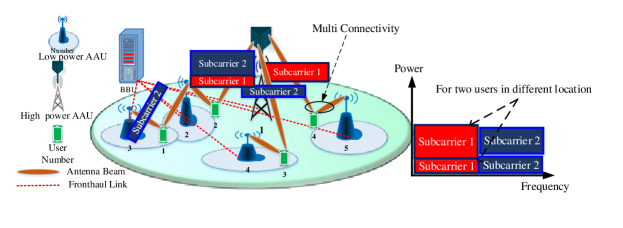
Figure 1: Schematic presentation of our designed MISO NOMA-enabled C-RAN and an example of the proposed SIC ordering algorithm.

In addition, $s_{k,n}^{f}$ is the signal of user $k$ over subcarrier $n$ from AAU $f$, and $\mathbb{w}_{k,n,f}=[w_{k,n,f}^{m}]\in\mathcal{C}^{M\times 1}$ is the vector of beamforming variables that is designed by AAU $f$ for user $k$ over subcarrier $n$.

Table I: Table of the main notations

Notation	Description
Notations/parameters
$\mathcal{F}/F/f$	Set/number/index of all AAUs in the network
$\mathcal{K}/K/k$	Set/number/index of all users in the network
$\mathcal{N}/N/n$	Set/number/index of the shared subcarriers in each AAU
${M}/m$	Number/index of antennas in each AAU
$P_{\text{max}}^{f}$	Maximum allowable transmit power of AAU $f$
$P_{\text{Total}}$	Total consumed power
$R_{\max}^{f}$	Maximum capacity of fronthaul link AAU $f$
$\mathbb{h}_{k,n,f}$	Real channel coefficient between user $k$
	and AAU $f$ on subcarrier $n$
$\tilde{\mathbb{h}}_{k,n,f}$	Estimated channel coefficient between user $k$
	and AAU $f$ on subcarrier $n$
$\bm{\epsilon}_{k,n,f}$	Channel estimation error for user $k$ and AAU $f$
	on subcarrier $n$
$\delta_{k,n}^{f}$	Channel uncertainty radius for user $k$ and AAU $f$
	on subcarrier $n$
$L_{n}^{f}$	Maximum reused number of each subcarrier $n$ at AAU $f$
${\sigma_{k,n,f}^{2}}$	Variance of noise at user $k$ on subcarrier $n$ from AAU $f$
$s_{k,n}^{f}$	Transmit signal at user $k$ on subcarrier $n$ from AAU $f$
$r_{k,n}^{f}$	Achieved rate of user $k$ on subcarrier $n$ from AAU $f$
$\varphi_{f}$	Preprocessing weight of each fronthual link of AAU $f$
$\beta$	Drain efficiency of the power amplifier
Optimization Variables
${\rho_{k,n}^{f}}$	Binary subcarrier assignment variables, equals to 1 means
	that user $k$ is scheduled to AAU $f$ and subcarrier $n$,
	otherwise, it is 0
$\xi_{i,n}^{k}$	Binary SIC ordering variable, which $\xi_{i,n}^{k}=1$, if user $k$
	decodes the signal of user $i$ on subcarrier $n$, else $\xi_{i,n}^{k}=0$
${\mathbb{w}_{k,n,f}}$	Beamforming vector from AAU $f$ to user $k$
	on subcarrier $n$

Let us define a joint subcarrier and user associations binary variable, $\rho_{k,n}^{f}$, if subcarrier $n$ is assigned to user $k$ that is served by $f$, $\rho_{k,n}^{f}=1$, otherwise, $\rho_{k,n}^{f}=0$. We introduce our scheduling policy in terms of subcarrier assignment technique and connectivity of users to AAUs as follows:
$\bullet$ Subcarrier Assignment as Multiple Access Technique: By exploiting NOMA, each subcarrier $n$ can be assigned to at most $L_{n}^{f}$ users in AAU $f$ which is ensured by

$$\sum_{k\in\mathcal{K}}\rho_{k,n}^{f}\leq L_{n}^{f},\,\forall n\in\mathcal{N},f\in\mathcal{F}.$$ (1)

$\bullet$ User Association as Connectivity Technique: In general, user association refers to find an algorithm to assign users to the radio stations. We propose a novel user association policy where each user can be configured to receive its data on different subcarriers from different AAUs. We call it multi-connectivity technique which is different from the coordinated multipoint technologies [30]. Therefore, each user on each subcarrier can be connected to at most one AAU which is ensured by the following constraint:

$${\sum_{f\in\mathcal{F}}\rho_{k,n}^{f}\leq 1,\forall n\in\mathcal{N},{k}\in\mathcal{K}}.$$ (2)

Let $\mathbb{h}_{k,n,f}\in\mathcal{C}^{M\times 1}$ be the channel coefficient between user $k$ and AAU $f$ on subcarrier $n$. Following channel uncertainty, i.e., imperfect CSI model, we assume that the global CSI is not known because of estimation errors and/or feedback delays [19, 38]. Therefore, the real channel gain is given as follows[19]:

$$\mathbb{h}_{k,n,f}=\tilde{\mathbb{h}}_{k,n,f}+\bm{\epsilon}_{k,n,f},\,\forall k,n,f,$$ (3)

where $\tilde{\mathbb{h}}_{k,n,f}$ denotes the estimated channel gain and $\bm{\epsilon}_{k,n,f}$ indicates the error of estimation which lies in a bounded spherical set as given by $\|\bm{\epsilon}_{k,n,f}\|_{2}^{2}\leq\delta_{k,n}^{f}$, where $\delta_{k,n}^{f}$ is the channel uncertainty radius and is assumed be a small constant [38, 46]. In the other words, we have $\mathbb{h}_{k,n,f}\in\mathcal{H}_{k,n,f}$, where $\mathcal{H}_{k,n,f}$ is as follows:

$$\mathcal{H}_{k,n,f}\triangleq\Big{\{}\tilde{\mathbb{h}}_{k,n,f}+\bm{\epsilon}_{k,n,f}\leavevmode\nobreak\ \big{|}\leavevmode\nobreak\ \|\bm{\epsilon}_{k,n,f}\|_{2}^{2}\leq\delta_{k,n}^{f}\Big{\}}.$$ (4)

The indispensable part of NOMA is the SIC algorithm which is applied in the receiver side to handle the NOMA interference. Since in NOMA, the SIC ordering has a key impact on the received signal to interference plus noise ratio (SINR), and the performance of NOMA for cell-edge or cell-central users [21], we devise a new SIC ordering method as follows:

II-A1 Proposed SIC Ordering Algorithm

In contrast to sorting users based on the channel condition to perform SIC, we introduce a new binary variable as $\xi_{i,n}^{k}$, where $\xi_{i,n}^{k}=1$ if user $k$ decodes the signal of user $i$ on the assigned subcarrier $n$ (assuming both users $k$ and $i$ are multiplexed on subcarrier $n$), and otherwise, $\xi_{i,n}^{k}=0$. Note that users $i$ and $k$ can be connected to different AAUs. It is worth noting that the traditional SIC ordering is based on the channel power gain, channel gain [6, 7, 14], and normalized noise power [45].
$\bullet$  Worst-Case Data Rate: The achievable rate of user $k$ on subcarrier $n$ and AAU $f$ with channel $\mathbb{h}_{k,n,f}$ is obtained by (5) shown at the top of next page.

$$r_{k,n}^{f}=\log_{2}\left(1+\frac{\rho_{k,n}^{f}|\mathbb{h}_{k,n,f}^{\dagger}\mathbb{w}_{k,n,f}|^{2}}{\sum\limits_{f^{\prime}\in\mathcal{F}}\sum\limits_{i\in\mathcal{K}\backslash\{k\}}\rho_{i,n}^{f^{\prime}}\cdot(1-\xi_{i,n}^{k})\cdot|\mathbb{h}_{k,n,f^{\prime}}^{\dagger}\mathbb{w}_{i,n,f^{\prime}}|^{2}+\sigma_{k,n,f}^{2}}\right),$$ (5)

 

The worst-case data rate of user $k$ over the uncertainty set can be formulated as

$$r_{k}=\sum_{f^{\prime}\in\mathcal{F}}\sum_{n\in\mathcal{N}}\min_{\Big{\{}\mathbb{h}_{k,n,f}\in\mathcal{H}_{k,n,f},\forall f\Big{\}}}r_{k,n}^{f^{\prime}},\leavevmode\nobreak\ \leavevmode\nobreak\ \forall k\in\mathcal{K}.$$ (6)

$\bullet\leavevmode\nobreak\$Successful Decoding Constraints as SIC Constraints: To ensure that user $k$ can successfully cancel the signal of user $i$, i.e., user $k$ is determined to perform SIC on subcarrier $n$ which means $\xi_{i,n}^{k}=1$, we consider the following three constraints should be satisfied, simultaneously.

1. SIC ordering variable can be $1$, when both users $k$ and $i$ are multiplexed on subcarrier $n$ which is ensured by

   $$\xi_{i,n}^{k}\leq\sum_{f\in\mathcal{F}}\rho_{k,n}^{f}\cdot\sum_{f^{\prime}\in\mathcal{F}}\rho_{i,n}^{f^{\prime}},\forall n\in\mathcal{N},\leavevmode\nobreak\ i\neq k,k,i\in\mathcal{K}.$$ (7)

2. Ensuring that one of the user $k$ or user $i$ performs SIC over the multiplexed subcarrier $n$ by

   $$\xi_{i,n}^{k}+\xi_{k,n}^{i}\leq 1,\leavevmode\nobreak\ \forall n\in\mathcal{N},k,i\in\mathcal{K},k\neq i.$$ (8)

3. Successful decoding constraint, which ensures that signal of user $i$ (connected to $f^{\prime}$) on subcarrier $n$ is detected and cancelled by user $k$ (connected to $f$) in the worst condition (based on (5)), is given by (9) shown at the top of the next page.

   $$\underbrace{\xi_{i,n}^{k}}_{\text{A}}\underbrace{\max_{\Big{\{}\mathbb{h}_{i,n,f}\in\mathcal{H}_{i,n,f},\forall f\Big{\}}}}_{\text{B}}\underbrace{\log_{2}\left(1+\frac{\rho_{i,n}^{f^{\prime}}|\mathbb{h}_{i,n,f^{\prime}}^{\dagger}\mathbb{w}_{i,n,f^{\prime}}|^{2}}{\sum_{f\in\mathcal{F}}\sum_{k^{\prime}\in\mathcal{K}\backslash\{i\}}\rho_{k^{\prime},n}^{f}(1-\xi_{k^{\prime},n}^{i})|\mathbb{h}_{i,n,f}^{\dagger}\mathbb{w}_{k^{\prime},n,f}|^{2}+\sigma_{i,n,f}^{2}}\right)}_{\text{C}}$$ (9)

   $$\leq\underbrace{\xi_{i,n}^{k}}_{\text{A}}\underbrace{\min_{\mathbb{h}_{k,n,f}\in\mathcal{H}_{k,n,f},\forall f}}_{\text{D}}\underbrace{\log_{2}\left(1+\frac{\rho_{i,n}^{f^{\prime}}|\mathbb{h}_{k,n,f^{\prime}}^{\dagger}\mathbb{w}_{i,n,f^{\prime}}|^{2}}{\sum_{f\in\mathcal{F}}\sum_{k^{\prime}\in\mathcal{K}\backslash\{i\}}\rho_{k^{\prime},n}^{f}(1-\xi_{k^{\prime},n}^{i})|\mathbb{h}_{k,n,f}^{\dagger}\mathbb{w}_{k^{\prime},n,f}|^{2}+\sigma_{k,n,f}^{2}}\right)}_{\text{E}}.$$

    

   In (9), part A ensures the constraint holds for user $k$ that is determined to perform SIC to decode and remove user $i$’s signal where both of them are multiplexed on subcarrier $n$. Parts B and D assure that the constraint holds for the worst-case estimation of CSI. To be clear, assume an example where we have two parameters as $a\in[a_{\min},a_{\max}]$ and $b\in[b_{\min},b_{\max}]$, and to ensure an inequality $a\leq b$ for all/worst-cases, obviously, it occurs for $a_{\max}\leq b_{\min}$. Part C is the obtained rate of user $i$ and part E is the rate of user $i$ achieved by user $k$ [20, 6, 7]. It should be noted that (9) is sufficient (but not necessary) for SIC.

II-A2 Fronthaul Link Capacity Constraints

Since the bandwidth of fronthaul links are limited, we introduce a new link capacity constraint as

$$\sum_{k\in\mathcal{K}}\sum_{n\in\mathcal{N}}\varphi_{f}\cdot r_{k,n}^{f}\leq R_{\max}^{f},\forall f\in\mathcal{F},$$ (10)

where $\varphi_{f}$ and $R_{\max}^{f},\forall f\in\mathcal{F}$ are the preprocessing weight related to the fronthaul transmission technologies and maximum available transmission capacity of AAU $f$, respectively.

II-B Objective Function and Problem Formulation

In this section, the considered objective function and problem formulation are introduced.

II-B1 Objective Function

Considering the worst-case channel uncertainties, the main goal of the optimization problem is to maximize the worst-case global EE (GEE) of the system. GEE is defined as the ratio of the global achievable sum rate to the total consumed power [40], and the worst-case of GEE is obtained with considering the worst-case CSI in our model. To formulate the worst-case EE, we need the worst-case throughput of the system and the total consumed power. The total worst-case data rate can be calculated by

$$R_{\text{Total}}^{\text{Worst}}=\sum_{k\in\mathcal{K}}r_{k}.$$ (11)

The total power consumption of the system is obtained by [31]

$$P_{\text{Total}}=\sum_{f\in\mathcal{F}}\underbrace{\sum_{k\in\mathcal{K}}\sum_{n\in\mathcal{N}}\frac{1}{\beta}\|\mathbb{w}_{k,n,f}\|_{2}^{2}}_{P_{\text{TX}}^{f}}+P_{\text{Static}},$$ (12)

where $0<\beta<1$ is the drain efficiency of the power amplifier and $P_{\text{Static}}$ is the static term of power consumption which is obtained as $P_{\text{Static}}=\sum_{f\in\mathcal{F}}P_{\text{Static}}^{f}$, where $P_{\text{Static}}^{f}$ is the static term of power which is given by

$$P_{\text{Static}}^{f}=\left\{\begin{array}[]{ll}P_{\text{Hardware}}^{f}&0<P_{\text{TX}}^{f}\leq P_{\max}^{f},\\ P_{\text{Sleep}}^{f}&P_{\text{TX}}^{f}=0,\end{array}\right.$$ (13)

where $P_{\text{Sleep}}^{f}$ is the consumed power at BBU in the sleep mode of AAU $f$ and $P_{\text{Hardware}}^{f}=C_{\text{Circuit}}\times M$ is the power that is used by hardware at AAU $f$ in the transmission mode, and $C_{\text{Circuit}}$ is the consumed circuit power constant that is used for the signal processing functions at AAU which includes the power dissipation in the filtering, frequency synthesizer, digital-to-analog converter, etc. Therefore, the worst-case EE of the system is calculated by

$$\eta_{\text{EE}}^{\text{Worst}}=\frac{R_{\text{Total}}^{\text{Worst}}}{P_{\text{Total}}},$$ (14)

where $R_{\text{Total}}^{\text{Worst}}$ and $P_{\text{Total}}$ are given by (11) and (12), respectively.

II-B2 Problem Formulation

Based on these definitions and assumptions, our main aim is to maximize the worst case of EE considering beamforming and SIC ordering constraints. The optimization problem is mathematically formulated as follows:

$$\max_{\mathbb{W},\bm{\xi},\bm{\rho}}\; \leavevmode\nobreak\ \eta_{\text{EE}}^{\text{Worst}}$$ (15a)

s.t. $$\text{C}_{1}:\sum_{k\in\mathcal{K}}\sum_{n\in\mathcal{K}}\rho_{k,n}^{f}\|\mathbb{w}_{k,n,f}\|_{2}^{2}\leq P_{\text{max}}^{f},\forall f\in\mathcal{F},$$ (15b)

$$\text{C}_{2}:\sum_{k\in\mathcal{K}}\rho_{k,n}^{f}\leq L_{n}^{f},\,\forall n\in\mathcal{N},f\in\mathcal{F},$$ (15c)

$$\text{C}_{3}:{\sum_{f\in\mathcal{F}}\rho_{k,n}^{f}\leq 1,\forall n\in\mathcal{N},{k}\in\mathcal{K}},$$ (15d)

$$\text{C}_{4}:\xi_{i,n}^{k},\rho_{k,n}^{f}\in\begin{Bmatrix}0,1\end{Bmatrix},\,\,\forall k\in\mathcal{K},n\in\mathcal{N},\forall f\in\mathcal{F},$$ (15e)

$$\eqref{SIC_Sub_Con},\eqref{SIC_Con_1},\eqref{SIC_Ordeing},\eqref{Fronthaul_Con},$$

where $\mathbb{W}=\left[{w}_{k,n,f}^{m}\right]$, $\bm{\rho}=\left[\rho_{k,n}^{f}\right]$,  and $\bm{\xi}=\left[\xi_{i,n}^{k}\right]$. Constraint (15b) indicates the maximum available power budget and constraint (15c) verifies that each subcarrier $n$ in each AAU $f$ can be utilized no more than $L_{n}^{f}$ times, recognized as NOMA constraint. Constraint (15d) ensures that each user on each subcarrier is served only by one AAU, (15e) stands for binary variables, and (7) indicates that the SIC on each subcarrier between users which are multiplexed on that subcarrier. Moreover, (8) indicates that for any two users only one of them can perform SIC on another one and (9) ensures that user $k$ decodes the message of user $i$ on the assigned subcarrier $n$, successfully [6, 22]. Finally, constraint (10) is the link capacity restriction of fronthaul links.

III Proposed Solution Methods

The optimization problem in (15) is a non-convex mixed integer non-linear programming (MINLP) which is complicated to solve. We propose two different solution algorithms which are discussed in the following.

III-A Algorithm 1: One Step Solution

In this section, we explain our proposed one-step solution, i.e., all variables are obtained without using alternating approach. First, let us define matrices $\mathbb{W}_{k,n,f}$ and $\tilde{\mathbb{H}}_{k,n,f}$ with size $M\times M$ as $\mathbb{W}_{k,n,f}\triangleq\mathbb{w}_{k,n,f}\mathbb{w}_{k,n,f}^{\dagger}$ and $\tilde{\mathbb{H}}_{k,n,f}\triangleq\tilde{\mathbb{h}}_{k,n,f}\tilde{\mathbb{h}}_{k,n,f}^{\dagger}$, respectively. To this end, we rewrite $\|\mathbb{h}_{k,n,f}^{\dagger}\mathbb{w}_{k,n,f}\|^{2}$ as follows:

$$\|\mathbb{h}_{k,n,f}^{\dagger}\mathbb{w}_{k,n,f}\|^{2}=$$

$$\mathbb{w}_{k,n,f}^{\dagger}(\tilde{\mathbb{h}}_{k,n,f}+\bm{\epsilon}_{k,n,f})^{\dagger}(\tilde{\mathbb{h}}_{k,n,f}+\bm{\epsilon}_{k,n,f})\mathbb{w}_{k,n,f}$$

$$=\mathbb{w}_{k,n,f}^{\dagger}(\tilde{\mathbb{h}}_{k,n,f}+\bm{\Delta}_{k,n,f})\mathbb{w}_{k,n,f}$$

$$=\text{Tr}[(\tilde{\mathbb{H}}_{k,n,f}+\bm{\Delta}_{k,n,f})\mathbb{W}_{k,n,f}],$$ (16)

where $\bm{\Delta}_{k,n,f}=\tilde{\mathbb{h}}_{k,n,f}\bm{\epsilon}_{k,n,f}^{\dagger}+\bm{\epsilon}_{k,n,f}\tilde{\mathbb{h}}_{k,n,f}+\bm{\epsilon}_{k,n,f}\bm{\epsilon}_{k,n,f}^{\dagger}$ is a norm-bounded matrix which satisfies the following region:

$$\|\bm{\Delta}_{k,n,f}\| \leq\|\tilde{\mathbb{h}}_{k,n,f}\bm{\epsilon}_{k,n,f}^{\dagger}\|+\|\bm{\epsilon}_{k,n,f}\tilde{\mathbb{h}}_{k,n,f}^{\dagger}\|+\|\bm{\epsilon}_{k,n,f}\bm{\epsilon}^{\dagger}_{k,n}\|,$$

$$\leq\|\tilde{\mathbb{h}}_{k,n,f}\|\|\bm{\epsilon}_{k,n,f}^{\dagger}\|+\|\bm{\epsilon}_{k,n,f}\|\|\tilde{\mathbb{h}}_{k,n,f}^{\dagger}\|$$

$$+\|\bm{\epsilon}_{k,n,f}\|\|\bm{\epsilon}^{\dagger}_{k,n}\|$$

$$=(\delta^{f}_{k,n})^{2}+2\delta_{k,n}^{f}\|\tilde{\mathbb{h}}_{k,n,f}\|\triangleq e_{k,n}^{f}.$$ (17)

Therefore, equation (5) can be rewritten as (18) shown at the top of the next page.

$${r}^{f}_{k,n}=\log_{2}\left(1+\frac{\rho_{k,n}^{f}\text{Tr}[(\tilde{\mathbb{H}}_{k,n,f}+\bm{\Delta}_{k,n,f})\mathbb{W}_{k,n,f}]}{\sum_{f^{\prime}\in\mathcal{F}}\sum_{i\in\mathcal{K}\backslash\{k\}}\rho_{i,n}^{f^{\prime}}(1-\xi_{i,n}^{k})\text{Tr}[(\tilde{\mathbb{H}}_{k,n,f^{\prime}}+\bm{\Delta}_{k,n,f^{\prime}})\mathbb{W}_{i,n,f^{\prime}}]+\sigma_{k,n,f}^{2}}\right).$$ (18)

 

Now, we aim at maximizing the worst-case data rate (18). Since the log function is a monotonic function, finding the worst-case would be done over the SINR in (18). This can be obtained by minimizing (18) over $\Delta_{k,n,f}$ and $\Delta_{k,n,f^{\prime}}$ where indexes $f$ and $f^{\prime}$ can be the same, i.e., when we calculate the intra-cell interference. One conservative method to find the minimum of the SINR is minimizing the numerator and maximizing the denominator of SINR in (18) with respect to norm-bounded matrices [49]. Note that by this method, we provide a strictly bounded robust solution (SBRS) [49]. Motivated by this idea, the lower bound of SINR in (18) subject to (III-A) can be obtained by solving the following optimization problems:

$$\min_{\|\bm{\Delta}_{k,n,f}\|\leq e_{k,n,f}}\text{Tr}[(\tilde{\mathbb{H}}_{k,n,f}+\bm{\Delta}_{k,n,f})\mathbb{W}_{k,n,f}],$$ (19)

$$\max_{\|\bm{\Delta}_{k,n,f^{\prime}}\|\leq e_{k,n,f^{\prime}}}\sum_{f^{\prime}\in\mathcal{F}}\sum_{i\in\mathcal{K}\backslash\{k\}}\text{Tr}[(\tilde{\mathbb{H}}_{k,n,f^{\prime}}+\bm{\Delta}_{k,n,f^{\prime}})\mathbb{W}_{i,n,f^{\prime}}].$$ (20)

Here, we apply the Lagrangian-based method to find the optimal solution of (19) and (20) for the given the beamforming matrices [49].

Proposition 1.

For the given $\mathbb{W}_{k,n,f}$, the minimum and maximum norm-bounded matrices of (19) and (20) given as follows, respectively, for all $k,i,n,f,f^{\prime}$:

$$\Delta^{f,\min}_{k,n}=-e_{k,n,f}\frac{\mathbb{W}^{\dagger}_{k,n,f}}{\|\mathbb{W}_{k,n,f}\|},\leavevmode\nobreak\ \forall k,n,f,$$ (21)

$$\Delta^{f^{\prime},\max}_{k,n}=e_{k,n,f^{\prime}}\frac{\mathbb{W}^{\dagger}_{i,n,f^{\prime}}}{\|\mathbb{W}_{i,n,f^{\prime}}\|},\leavevmode\nobreak\ \forall k,i\in\mathcal{K},n,f,k\neq i.$$ (22)

Proof.

Please see Appendix A. ∎

The following remark provides the exact solution for the worst-case of SINR.

Remark 1.

The exact worst-case of the SINR can be obtained by using the fractional programming. The minimization of the SINR over a bounded error is a fractional program as follows:

$$\min_{\|\bm{\Delta}_{k,n,f}\|\leq e_{k,n,f}}$$ (23)

$$\frac{\text{Tr}[(\tilde{\mathbb{H}}_{k,n,f}+\bm{\Delta}_{k,n,f})\mathbb{W}_{k,n,f}]}{\sum_{f^{\prime}\in\mathcal{F}}\sum_{i\in\mathcal{K}\backslash\{k\}}\text{Tr}[(\tilde{\mathbb{H}}_{k,n,f^{\prime}}+\bm{\Delta}_{k,n,f^{\prime}})\mathbb{W}_{i,n,f^{\prime}}]+\sigma_{k,n,f}^{2}}.$$

The solution of (23) can be obtained using the idea of fractional programming. This method provides a numerical solution for the worst-case $\Delta_{k,n,f}$. Hence, by idea of fractional programming, we restate (23) in parametric form as:

$$\min_{\|\bm{\Delta}_{k,n,f}\|\leq e_{k,n,f}}F(\bm{\Delta}_{k,n,f},\nu),$$ (24)

where

$$F(\bm{\Delta}_{k,n,f},\nu)\triangleq{\text{Tr}[(\tilde{\mathbb{H}}_{k,n,f}+\bm{\Delta}_{k,n,f})\mathbb{W}_{k,n,f}]}$$ (25)

$$-\nu\Big{(}{\sum_{f^{\prime}\in\mathcal{F}}\sum_{i\in\mathcal{K}\backslash\{k\}}\text{Tr}[(\tilde{\mathbb{H}}_{k,n,f^{\prime}}+\bm{\Delta}_{k,n,f^{\prime}})\mathbb{W}_{i,n,f^{\prime}}]+\sigma_{k,n,f}^{2}}\Big{)},$$

and $\nu$ is an auxiliary variable updated in each iteration of Dinkelbach algorithm by

$$\nu=$$ (26)

$$\frac{\text{Tr}[(\tilde{\mathbb{H}}_{k,n,f}+\bm{\Delta}_{k,n,f}^{*})\mathbb{W}_{k,n,f}]}{{\sum_{f^{\prime}\in\mathcal{F}}\sum_{i\in\mathcal{K}\backslash\{k\}}\text{Tr}[(\tilde{\mathbb{H}}_{k,n,f^{\prime}}+\bm{\Delta}_{k,n,f^{\prime}}^{*})\mathbb{W}_{i,n,f^{\prime}}]+\sigma_{k,n,f}^{2}}},$$

where $\bm{\Delta}_{k,n,f}^{*}$ is obtained by (28) which will be explained next. In each iteration of the Dinkelbach algorithm, we need to obtain $\text{argmin}_{\|\bm{\Delta}_{k,n,f}\|\leq e_{k,n,f}}F(\bm{\Delta}_{k,n,f},q)$. We adopt the Lagrangian method. To this end, we define the Lagrangian function as follows:

$$\mathcal{L}(\bm{\Delta}_{k,n,f})=F(\bm{\Delta}_{k,n,f},\nu)+\Omega(\|\bm{\Delta}_{k,n,f}\|-e_{k,n,f}),$$ (27)

where $\Omega$ is the Lagrangian multiplier. Taking the derivations of (27) with respect to $\bm{\Delta}_{k,n,f}$ and $\Omega$, and setting their values to zero, we obtain $\bm{\Delta}_{k,n,f}^{*}$ as follows:

$$\bm{\Delta}_{k,n,f}^{*}=\text{argmin}_{\mathcal{L}(\bm{\Delta}_{k,n,f})}.$$ (28)

The update procedure in Dinkelbach algorithm is proceed until the convergence condition is met. We call this method as exact robust solution (ExRS). It is worthwhile mentioning that, since the objective function in (23) is pseudo-linear, we can solve the max (best-case) using the same approach.

By substituting (21) and (22) into the data rate (18), we obtain (29),

$$\tilde{r}_{k,n}^{f}=\log_{2}\bigg{(}1+\frac{\rho_{k,n}^{f}\big{(}\text{Tr}[\tilde{\mathbb{H}}_{k,n,f}\mathbb{W}_{k,n,f}]-e_{k,n}^{f}{\|\mathbb{W}_{k,n,f}\|}\big{)}}{\sum_{f^{\prime}\in\mathcal{F}}\sum_{i\in\mathcal{K}\backslash\{k\}}\rho_{i,n}^{f^{\prime}}(1-\xi_{i,n}^{k})\big{\{}\text{Tr}[\tilde{\mathbb{H}}_{k,n,f^{\prime}}\mathbb{W}_{i,n,f^{\prime}}]+e_{k,n}^{f^{\prime}}{\|\mathbb{W}_{i,n,f^{\prime}}\|}\big{\}}+\sigma_{k,n,f}^{2}}\bigg{)}.$$ (29)

 

where $\tilde{r}_{k,n}^{f}$ is the lower bound on the worst-case data rate. Therefore, the total data rate for the worst-case is given by

$$R_{\text{Total}}^{\text{Worst}}=\sum_{f\in\mathcal{F}}\sum_{k\in\mathcal{K}}\sum_{n\in\mathcal{N}}\tilde{r}_{k,n}^{f}.$$ (30)

Moreover, we restate the constraint (9) by using Proposition 1 as (31) shown at top of the next page which may not be tight.

$$\log_{2}\bigg{(}1+\frac{\xi_{i,n}^{k}\rho_{i,n}^{f^{\prime}}\big{\{}\text{Tr}[\tilde{\mathbb{H}}_{i,n,f^{\prime}}\mathbb{W}_{i,n,f^{\prime}}]+e_{i,n}^{f^{\prime}}{\|\mathbb{W}_{i,n,f^{\prime}}\|}\big{\}}}{\sum_{f\in\mathcal{F}}\sum_{k^{\prime}\in\mathcal{K}\backslash\{i\}}\rho_{k^{\prime},n}^{f}(1-\xi_{k^{\prime},n}^{i})\big{\{}\text{Tr}[\tilde{\mathbb{H}}_{i,n,f}\mathbb{W}_{k^{\prime},n,f}]-e_{i,n}^{f}{\|\mathbb{W}_{k^{\prime},n,f}\|}\big{\}}+\sigma_{i,n,f^{\prime}}^{2}}\bigg{)}$$ (31)

$$\leq\log_{2}\bigg{(}1+\frac{\xi_{i,n}^{k}\rho_{i,n}^{f^{\prime}}\big{\{}\text{Tr}[\tilde{\mathbb{H}}_{k,n,f^{\prime}}\mathbb{W}_{i,n,f^{\prime}}]-e_{k,n}^{f^{\prime}}{\|\mathbb{W}_{i,n,f^{\prime}}\|}\big{\}}}{\sum_{f\in\mathcal{F}}\sum_{k^{\prime}\in\mathcal{K}\backslash\{i\}}\rho_{k^{\prime},n}^{f}(1-\xi_{k^{\prime},n}^{i})\{\text{Tr}[\tilde{\mathbb{H}}_{k,n,f}\mathbb{W}_{k^{\prime},n,f}]+e_{k,n}^{f}{\|\mathbb{W}_{k^{\prime},n,f}\|}\}+\sigma_{k,n,f}^{2}}\bigg{)}.$$

 

In (31), the left hand side is obtained for the maximum while the right hand side is obtained for the minimum. We also note that the term $\{\xi_{i,n}^{k}\cdot\rho_{i,n}^{f^{\prime}}\}$ in (29) is non-convex. To tackle this issue, we define a new variable as the multiplication of two binary variables $x_{i,n}^{k,f^{\prime}}=\xi_{i,n}^{k}\cdot\rho_{i,n}^{f^{\prime}}$, which indicates the joint SIC ordering and scheduling variables. Then, we adopt a linearizion technique and add the following constraints to the optimization problem [51, 50]:

$$\text{C}_{7}:\leavevmode\nobreak\ \xi_{i,n}^{k}\geq x_{i,n}^{k,f},\leavevmode\nobreak\ \forall k,i\in\mathcal{K},n\in\mathcal{N},f\in\mathcal{F},$$ (32)

$$\text{C}_{8}:\leavevmode\nobreak\ \rho_{i,n}^{f}\geq x_{i,n}^{k,f},\leavevmode\nobreak\ \forall k,i\in\mathcal{K},n\in\mathcal{N},f\in\mathcal{F},$$ (33)

$$\text{C}_{9}:\leavevmode\nobreak\ \rho_{i,n}^{f}+\xi_{i,n}^{k}-1\leq x_{i,n}^{k,f},\forall k,i\in\mathcal{K},n\in\mathcal{N},f\in\mathcal{F}.$$ (34)

Furthermore, in order to handle the non-convex integer variables in problem (15), we rewrite the constraint (15e) as the intersection of the following regions:

$$\text{C}_{10}:0\leq\xi_{i,n}^{k}\leq 1,\leavevmode\nobreak\ \text{C}_{11}:\sum_{i,k\in\mathcal{K}}\sum_{n\in\mathcal{N}}\bigg{(}\xi_{i,n}^{k}-(\xi_{i,n}^{k})^{2}\bigg{)}\leq 0,$$

$$\text{C}_{12}:0\leq\rho_{k,n}^{f}\leq 1,\leavevmode\nobreak\$$

$$\text{C}_{13}:\sum_{f\in\mathcal{F}}\sum_{k\in\mathcal{K}}\sum_{n\in\mathcal{N}}\bigg{(}\rho_{k,n}^{f}-(\rho_{k,n}^{f})^{2}\bigg{)}\leq 0,$$

$$\text{C}_{14}:0\leq x_{i,n}^{k,f}\leq 1,$$

$$\text{C}_{15}:\sum_{f\in\mathcal{F}}\sum_{i,k\in\mathcal{K}}\sum_{n\in\mathcal{N}}\bigg{(}x_{i,n}^{k,f}-(x_{i,n}^{k,f})^{2}\bigg{)}\leq 0.$$

Now, we rewrite the optimization problem as:

$$\max_{\mathbb{W},\bm{\xi},\bm{\rho}}\; \leavevmode\nobreak\ \eta_{\text{EE}}^{\text{Worst}}$$ (35a)

s.t. $$\text{C}_{1}:\sum_{k\in\mathcal{K}}\sum_{n\in\mathcal{K}}\text{Tr}[\rho_{k,n}^{f}\mathbb{W}_{k,n,f}]\leq P^{f}_{\text{max}},$$ (35b)

$$\text{C}_{2}:\sum_{k\in\mathcal{K}}\rho_{k,n}^{f}\leq L_{n}^{f},$$ (35c)

$$\text{C}_{3}:\mathbb{W}_{k,n,f}\succeq\mathbb{0},$$ (35d)

$$\text{C}_{4}:\text{Rank}(\mathbb{W}_{k,n,f})\leq 1,$$ (35e)

$$\text{C}_{7}-\text{C}_{15},$$ (35f)

$$\eqref{User_Assosiaction_2},\eqref{SIC_Sub_Con},\eqref{SIC_Con_1},\eqref{Fronthaul_Con},\eqref{SIC_C}.$$ (35g)

It can be concluded from the optimization problem (35), the product term of $\rho_{k,n}^{f}\mathbb{W}_{k,n,f}$ is an obstacle for solving the optimization problem. Let us define two new auxiliary variables as follows:

$$\tilde{\mathbb{W}}_{k,n,f}\triangleq\rho_{k,n}^{f}\mathbb{W}_{k,n,f},\leavevmode\nobreak\ \leavevmode\nobreak\ {\mathbb{W^{\prime}}}_{i,k,n,f}\triangleq x_{i,n}^{k,f}\mathbb{W}_{i,n,f}.$$

Also, we employ the big-M method [39, 14] to circumvent this difficulty. In particular, we impose the following additional constraints to make it convex as follows:

$$\text{C}_{16}:\leavevmode\nobreak\ \tilde{\mathbb{W}}_{k,n,f}\preceq P_{\text{max}}^{f}\mathbb{I}_{M}\rho_{k,n}^{f},$$ (36)

$$\text{C}_{17}:\leavevmode\nobreak\ \tilde{\mathbb{W}}_{k,n,f}\preceq\mathbb{W}_{k,n,f},\leavevmode\nobreak\ \text{C}_{18}:\leavevmode\nobreak\ \tilde{\mathbb{W}}_{k,n,f}\succeq\mathbb{0},$$ (37)

$$\text{C}_{19}:\leavevmode\nobreak\ \tilde{\mathbb{W}}_{k,n,f}\succeq\mathbb{W}_{k,n,f}-(1-\rho_{k,n}^{f})P_{\text{max}}^{f}\mathbb{I}_{M},$$ (38)

$$\text{C}_{20}:\leavevmode\nobreak\ {\mathbb{W^{\prime}}}_{i,k,n,f}\preceq P_{\text{max}}^{f}\mathbb{I}_{M}\leavevmode\nobreak\ x_{i,n}^{k,f},$$ (39)

$$\text{C}_{21}:\leavevmode\nobreak\ {\mathbb{W}^{\prime}}_{i,k,n,f}\preceq\mathbb{W}_{k,n,f},\leavevmode\nobreak\ \text{C}_{22}:\leavevmode\nobreak\ {\mathbb{W}^{\prime}}_{i,k,n,f}\succeq\mathbb{0},$$ (40)

$$\text{C}_{23}:\leavevmode\nobreak\ {\mathbb{W}^{\prime}}_{i,k,n,f}\succeq\mathbb{W}_{k,n,f}-(1-x_{i,n}^{k,f})P_{\text{max}}^{f}\mathbb{I}_{M}.$$ (41)

The worst-case data rate (30) and constraint (31) are still non-convex. To handle these and facilitate the solution, (30) can be rewritten as

$$R_{\text{Tota}}^{\text{Worst}}=\log_{2}\prod_{f\in\mathcal{F}}\prod_{k\in\mathcal{K}}\prod_{n\in\mathcal{N}}\frac{\psi_{f,k,n}}{\phi_{f,k,n}},$$ (42)

where

$$\psi_{f,k,n}=\text{Tr}[\tilde{\mathbb{H}}_{k,n,f}\tilde{\mathbb{W}}_{k,n,f}]-e_{k,n}^{f}\big{(}\mathcal{A}(\tilde{\mathbb{W}}_{k,n,f})\big{)}+\phi_{f,k,n},$$

$$\phi_{f,k,n}=$$

$$\sum_{f^{\prime}\in\mathcal{F}}\sum_{i\in\mathcal{K}\backslash\{k\}}\text{Tr}[\tilde{\mathbb{H}}_{k,n,f^{\prime}}\tilde{\mathbb{W}}_{i,n,f^{\prime}}]-\text{Tr}[\tilde{\mathbb{H}}_{k,n,f^{\prime}}{\mathbb{W}^{\prime}}_{i,k,n,f^{\prime}}]$$

$$+e_{k,n}^{f^{\prime}}\Big{(}\mathcal{A}(\tilde{\mathbb{W}}_{i,n,f^{\prime}})-\mathcal{B}(\mathbb{W}^{\prime}_{i,k,n,f^{\prime}})\Big{)}+\sigma^{2}_{k,n,f},$$ (43)

where we define

$$\mathcal{A}(\tilde{\mathbb{W}}_{k,n,f})\triangleq\|\rho_{k,n}^{f}\mathbb{W}_{k,n,f}\|={\|\tilde{\mathbb{W}}_{k,n,f}\|},$$ (44)

$$\mathcal{B}(\mathbb{W}^{\prime}_{i,k,n,f^{\prime}})\triangleq\|x_{i,n}^{k,f^{\prime}}\mathbb{W}_{i,n,f^{\prime}}\|=\|{\mathbb{W}^{\prime}}_{i,k,n,f^{\prime}}\|.$$ (45)

However, the total data rate (42) is still non-convex. Let us define

$$\psi_{f,k,n}\triangleq\exp({a_{f,k,n}}),\leavevmode\nobreak\ \phi_{f,k,n}\triangleq\exp({b_{f,k,n}}),$$ (46)

where $a_{f,k,n}$ and $b_{f,k,n}$ are slack variables. Moreover, the lower bound of slack variables have the following form [48]

$$\exp({a_{f,k,n}})\geq\sigma^{2}_{k,n,f},\leavevmode\nobreak\ \exp({b_{f,k,n}})\geq\sigma^{2}_{k,n,f}.$$ (47)

Now, by substituting (46) into the objective function, we can obtain

$$\max_{\mathbb{W},\mathbb{W^{\prime}},\tilde{\mathbb{W}},\bm{\xi},\bm{\rho},\mathbb{x}}\; \leavevmode\nobreak\ \frac{\log_{2}\prod_{f}\prod_{k}\prod_{n}\frac{\psi_{f,k,n}}{\phi_{f,k,n}}}{P_{\text{Total}}(\mathbb{W})}$$

$$=\max_{\mathbb{W},\mathbb{W^{\prime}},\tilde{\mathbb{W}},\bm{\xi},\bm{\rho},\mathbb{x},\mathbb{a},\mathbb{b}} \frac{\log_{2}\prod_{f}\prod_{k}\prod_{n}\exp({a_{f,k,n}}-b_{f,k,n})}{P_{\text{Total}}(\mathbb{W})}$$

$$=\max_{\mathbb{W},\mathbb{W^{\prime}},\tilde{\mathbb{W}},\bm{\xi},\bm{\rho},\mathbb{x},\mathbb{a},\mathbb{b}} \frac{\sum\limits_{f\in\mathcal{F}}\sum\limits_{k\in\mathcal{K}}\sum\limits_{n\in\mathcal{N}}({a_{f,k,n}}-b_{f,k,n})\log_{2}(e)}{P_{\text{Total}}(\mathbb{W})},$$

where $\mathbb{a}=[a_{f,k,n}]$ and $\mathbb{b}=[b_{f,k,n}]$ are the collection vectors of slack variables. Also, $P_{\text{Total}}(\mathbb{W})=\sum_{f\in\mathcal{F}}\sum_{k\in\mathcal{K}}\sum_{n\in\mathcal{N}}\frac{1}{\beta}\text{Tr}[\mathbb{W}_{k,n,f}]+P_{\text{Static}}$. For notation simplicity, let define $\Xi\triangleq\left[\mathbb{W^{\prime}},\tilde{\mathbb{W}},{\mathbb{W}},\bm{\xi},\bm{\rho},\mathbb{x},\mathbb{a},\mathbb{b}\right]$ as the collection of the optimization variables. It is worthwhile to mention that by this method, we can easily rewrite the non-convex constraint (10) as follows:

$$\sum_{k\in\mathcal{K}}\sum_{n\in\mathcal{N}}\varphi_{f}(a_{f,k,n}-b_{f,k,n})\leq R_{\max}^{f},\forall f\in\mathcal{F}.$$ (48)

Now, the optimization problem at hand can be mathematically formulated as

$$\max_{\Xi}$$ (49a)

$$\frac{\sum\limits_{f\in\mathcal{F}}\sum\limits_{k\in\mathcal{K}}\sum\limits_{n\in\mathcal{N}}({a_{f,k,n}}-b_{f,k,n})\log_{2}(e)}{P_{\text{Total}}(\mathbb{W})}+h(\bm{\xi},\bm{\rho},\mathbb{x},\lambda)$$ (49b)

s.t. $$\text{C}_{1}:\sum_{k\in\mathcal{K}}\sum_{n\in\mathcal{K}}\text{Tr}[\tilde{\mathbb{W}}_{k,n,f}]\leq P^{f}_{\text{max}},\leavevmode\nobreak\$$ (49c)

$$\text{C}_{2}:\sum_{k\in\mathcal{K}}\rho_{k,n}^{f}\leq L_{n}^{f},\,$$ (49d)

$$\text{C}_{3}:\mathbb{W}_{k,n,f}\succeq\mathbb{0},$$ (49e)

$$\text{C}_{4}:\text{Rank}(\mathbb{W}_{k,n,f})\leq 1,$$ (49f)

$$\exp({a_{f,k,n}})\geq\sigma^{2}_{k,n,f},\leavevmode\nobreak\ \exp({b_{f,k,n}})\geq\sigma^{2}_{k,n,f},$$ (49g)

$$a_{f,k,n}\geq b_{f,k,n},$$ (49h)

$$\psi_{f,k,n}\geq\exp(a_{f,k,n}),\leavevmode\nobreak\ \phi_{f,k,n}\leq\exp(b_{f,k,n}),$$ (49i)

$$\text{C}_{7}-\text{C}_{10},\text{C}_{12},\text{C}_{14},\text{C}_{16}-\text{C}_{23},$$ (49j)

$$\eqref{User_Assosiaction_2},\eqref{SIC_Sub_Con},\eqref{SIC_Con_1},\eqref{Fronthaul_Con},\eqref{SIC_C},$$ (49k)

where $h(\bm{\xi},\bm{\rho},\mathbb{x},\lambda)\triangleq-f(\bm{\xi},\bm{\rho},\mathbb{x},\lambda)+g(\bm{\xi},\bm{\rho},\mathbb{x},\lambda)$ is the penalty function. Furthermore, $f(\bm{\xi},\bm{\rho},\mathbb{x},\lambda)$ and $g(\bm{\xi},\bm{\rho},\mathbb{x},\lambda)$ are defined as

$$f(\bm{\xi},\bm{\rho},\mathbb{x},\lambda)\triangleq$$

$$\lambda\Bigg{(}\sum_{i,k\in\mathcal{K}}\sum_{n\in\mathcal{N}}\xi_{i,n}^{k}+\sum_{f\in\mathcal{F}}\sum_{k\in\mathcal{K}}\sum_{n\in\mathcal{N}}\rho_{k,n}^{f}+\sum_{f\in\mathcal{F}}\sum_{i,k\in\mathcal{K}}\sum_{n\in\mathcal{N}}x_{i,n}^{k,f}\Bigg{)},$$ (50)

$$g(\bm{\xi},\bm{\rho},\mathbb{x},\lambda)\triangleq\lambda\Bigg{(}\sum_{i,k\in\mathcal{K}}\sum_{n\in\mathcal{N}}(\xi_{i,n}^{k})^{2}$$

$$+\sum_{f\in\mathcal{F}}\sum_{k\in\mathcal{K}}\sum_{n\in\mathcal{N}}(\rho_{k,n}^{f})^{2}+\sum_{f\in\mathcal{F}}\sum_{i,k\in\mathcal{K}}\sum_{n\in\mathcal{N}}(x_{i,n}^{k,f})^{2}\Bigg{)},$$ (51)

respectively. It is worth mentioning that $\lambda$ indicates a penalty factor to penalize the objective function for any $\xi_{i,n}^{k}$, $\rho_{k,n}^{f}$, and $x_{k,n}^{f}$ which are not binary (i.e., their values are in $[0,1]$) [33]. However, the precise $0$ and $1$ are not always available. In this case, we round their values to the nearest integer values. The following proposition provides a mathematical analysis of the penalty factor.

Proposition 2.

For sufficiently large value of $\lambda$, we have $\min_{\lambda}\max_{\mathbb{W},\bm{\xi},\bm{\rho},\mathbb{x}}\mathcal{L}(\mathbb{W},\bm{\xi},\bm{\rho},\mathbb{x})=\max_{\mathbb{W},\bm{\xi},\bm{\rho},\mathbb{x}}\min_{\lambda}\mathcal{L}(\mathbb{W},\bm{\xi},\bm{\rho},\mathbb{x})$. In other words, the optimization problem (35) is equivalent to (49) where both problems obtain the same values.

Proof.

Please see Appendix B. ∎

Problem (49) is non-convex due to the constraints (49i) and (31) and $g(\bm{\xi},\bm{\rho},\mathbb{x},\lambda)$ in the objective function. In order to convert it into a convex one, we employ MM approach where a surrogate function is approximated by the first order Taylor approximation. Therefore, we use the following inequalities:

$$g(\bm{\xi},\bm{\rho},\mathbb{x},\lambda) \leq g(\bm{\xi}^{t-1},\bm{\rho}^{t-1},\mathbb{x}^{t-1},\lambda)$$

$$+\nabla_{\bm{\xi}}g^{T}(\bm{\xi}^{t-1},\bm{\rho}^{t-1},\mathbb{x}^{t-1},\lambda)(\bm{\xi}-\bm{\xi}^{t-1})$$

$$+\nabla_{\bm{\rho}}g^{T}(\bm{\xi}^{t-1},\bm{\rho}^{t-1},\mathbb{x}^{t-1},\lambda)(\bm{\rho}-\bm{\rho}^{t-1})$$

$$+\nabla_{\mathbb{x}}g^{T}(\bm{\xi}^{t-1},\bm{\rho}^{t-1},\mathbb{x}^{t-1},\lambda)(\mathbb{x}-\mathbb{x}^{t-1})$$

$$\triangleq\tilde{g}(\bm{\xi},\bm{\rho},\mathbb{x},\lambda),$$ (52)

$$\mathcal{A}(\tilde{\mathbb{W}}_{k,n,f})\leq\mathcal{A}(\tilde{\mathbb{W}}_{k,n,f})^{t-1}$$

$$+\text{Tr}\Big{(}\nabla_{\tilde{\mathbb{W}}_{k,n,f}}\mathcal{A}(\tilde{\mathbb{W}}_{k,n,f})^{t-1}[\mathcal{A}(\tilde{\mathbb{W}}_{k,n,f})^{t}-\mathcal{A}(\tilde{\mathbb{W}}_{k,n,f})^{t-1}]\Big{)}$$

$$\triangleq\tilde{\mathcal{A}}(\tilde{\mathbb{W}}_{k,n,f}),$$ (53)

$$\mathcal{B}(\mathbb{W}^{\prime}_{i,k,n,f^{\prime}})\leq\mathcal{B}(\mathbb{W}^{\prime}_{i,k,n,f^{\prime}})^{t-1}$$

$$+\text{Tr}\Big{(}\nabla_{\mathbb{W}^{\prime}_{i,k,n,f^{\prime}}}\mathcal{B}(\mathbb{W}^{\prime}_{i,k,n,f^{\prime}})^{t-1}\big{[}\mathcal{B}(\mathbb{W}^{\prime}_{i,k,n,f^{\prime}})^{t}$$

$$-\mathcal{B}(\mathbb{W}^{\prime}_{i,k,n,f^{\prime}})^{t-1}\big{]}\Big{)}\triangleq\tilde{\mathcal{B}}(\mathbb{W}^{\prime}_{i,k,n,f^{\prime}}),$$ (54)

$$\phi_{f,k,n}\leq\exp(b^{t-1}_{f,k,n})(b_{f,k,n}^{t}-b^{t-1}_{f,k,n}+1)\triangleq\tilde{\phi}_{f,k,n}.$$ (55)

It should be noted that the right hand sides of (III-A)-(54) are affine functions. Now the main challenge in problem (49) is the non-convex constraint (31), i.e., SIC ordering constraint. Next, we handle this constraint similar to the objective function. To this end, first, we rewrite (31) as (56) shown at the top of the next page, by replacing the previously defined auxiliary variables $x_{i,n}^{k,f^{\prime}}=\xi_{i,n}^{k}\cdot\rho_{i,n}^{f^{\prime}}$, $\tilde{\mathbb{W}}_{k,n,f}=\rho_{k,n}^{f}\mathbb{W}_{k,n,f},$ ${\mathbb{W^{\prime}}}_{i,k,n,f}=x_{i,n}^{k,f}\mathbb{W}_{i,n,f}$, (44), and (45).

$$\log_{2}\bigg{(}1+\frac{\text{Tr}[\tilde{\mathbb{H}}_{i,n,f^{\prime}}{\mathbb{W^{\prime}}}_{i,k,n,f^{\prime}}]+e_{i,n}^{f^{\prime}}{\mathcal{B}({\mathbb{W^{\prime}}}_{i,k,n,f^{\prime}})}}{\sum_{f\in\mathcal{F}}\sum_{k^{\prime}\in\mathcal{K}\backslash\{i\}}\Big{\{}\text{Tr}[\tilde{\mathbb{H}}_{i,n,f}\tilde{\mathbb{W}}_{k^{\prime},n,f}]-e_{i,n}^{f}{\mathcal{A}(\tilde{\mathbb{W}}_{k^{\prime},n,f})}-\big{\{}\text{Tr}[\tilde{\mathbb{H}}_{i,n,f}\mathbb{W^{\prime}}_{i,k^{\prime},n,f}]-e_{i,n}^{f}\mathcal{B}(\mathbb{W^{\prime}}_{i,k^{\prime},n,f})\big{\}}\Big{\}}+\sigma_{i,n,f^{\prime}}^{2}}\bigg{)}$$ (56)

$$\leq\log_{2}\bigg{(}1+\frac{\text{Tr}[\tilde{\mathbb{H}}_{k,n,f^{\prime}}\mathbb{W^{\prime}}_{i,k,n,f^{\prime}}]-e_{k,n}^{f^{\prime}}{\mathcal{B}({\mathbb{W^{\prime}}}_{i,k,n,f^{\prime}})}}{{\sum_{f\in\mathcal{F}}\sum_{k^{\prime}\in\mathcal{K}\backslash\{i\}}\Big{\{}\text{Tr}[\tilde{\mathbb{H}}_{k,n,f}\tilde{\mathbb{W}}_{k^{\prime},n,f}]+e_{i,n}^{f}{\mathcal{A}(\tilde{\mathbb{W}}_{k^{\prime},n,f})}-\big{\{}\text{Tr}[\tilde{\mathbb{H}}_{i,n,f}\mathbb{W^{\prime}}_{i,k^{\prime},n,f}]+e_{i,n}^{f}\mathcal{B}(\mathbb{W^{\prime}}_{i,k^{\prime},n,f})\big{\}}\Big{\}}+\sigma_{k,n,f}^{2}}}\bigg{)}.$$

 

Now, we can rewrite (56) as follows:

$$\log_{2}(\frac{\mathcal{D}_{i,k,n,f^{\prime}}}{\mathcal{E}_{i,n,f^{\prime}}})-\log_{2}(\frac{\mathcal{F}_{i,k,n,f^{\prime}}}{\mathcal{G}_{i,k,n,f^{\prime}}})\leq 0,$$ (57)

where

$$\mathcal{E}_{i,n,f^{\prime}}=\sum_{f\in\mathcal{F}}\sum_{k^{\prime}\in\mathcal{K}\backslash\{i\}}\Big{\{}\text{Tr}[\tilde{\mathbb{H}}_{i,n,f}\tilde{\mathbb{W}}_{k^{\prime},n,f}]-e_{i,n}^{f}{\mathcal{A}(\tilde{\mathbb{W}}_{k^{\prime},n,f})}$$

$$-\big{\{}\text{Tr}[\tilde{\mathbb{H}}_{i,n,f}\mathbb{W^{\prime}}_{i,k^{\prime},n,f}]-e_{i,n}^{f}\mathcal{B}(\mathbb{W^{\prime}}_{i,k^{\prime},n,f})\big{\}}\Big{\}}+\sigma_{i,n,f^{\prime}}^{2},$$ (58)

$$\mathcal{D}_{i,k,n,f^{\prime}}=$$

$$\text{Tr}[\tilde{\mathbb{H}}_{i,n,f^{\prime}}{\mathbb{W^{\prime}}}_{i,k,n,f^{\prime}}]+e_{i,n}^{f^{\prime}}{\mathcal{B}({\mathbb{W^{\prime}}}_{i,k,n,f^{\prime}})}+E_{i,n,f^{\prime}},$$ (59)

$$\mathcal{G}_{i,k,n,f^{\prime}}=\sum_{f\in\mathcal{F}}\sum_{k^{\prime}\in\mathcal{K}\backslash\{i\}}\text{Tr}[\tilde{\mathbb{H}}_{k,n,f}\tilde{\mathbb{W}}_{k^{\prime},n,f}]+e_{i,n}^{f}{\mathcal{A}(\tilde{\mathbb{W}}_{k^{\prime},n,f})}$$

$$-\big{\{}\text{Tr}[\tilde{\mathbb{H}}_{i,n,f}\mathbb{W^{\prime}}_{i,k^{\prime},n,f}]+e_{i,n}^{f}\mathcal{B}(\mathbb{W^{\prime}}_{i,k^{\prime},n,f})\big{\}}+\sigma_{k,n,f}^{2},$$ (60)

$$\mathcal{F}_{i,k,n,f^{\prime}}=$$

$$\mathcal{G}_{i,k,n,f^{\prime}}+\text{Tr}[\tilde{\mathbb{H}}_{k,n,f^{\prime}}\mathbb{W^{\prime}}_{i,k,n,f^{\prime}}]-e_{k,n}^{f^{\prime}}{\mathcal{B}({\mathbb{W^{\prime}}}_{i,k,n,f^{\prime}})}.$$ (61)

Hereafter, we drop the subscripts of $\mathcal{E}_{i,n,f^{\prime}},\leavevmode\nobreak\ \mathcal{D}_{i,k,n,f^{\prime}},\leavevmode\nobreak\ \mathcal{G}_{i,k,n,f^{\prime}},\leavevmode\nobreak\ \text{and}\leavevmode\nobreak\ \mathcal{F}_{i,k,n,f^{\prime}}$ for the notation simplicity and denote them by $\mathcal{E},\leavevmode\nobreak\ \mathcal{D},\leavevmode\nobreak\ \mathcal{G}$, and $\mathcal{F}$, respectively. After this, similar to (46), we consider the following definitions:

$$\mathcal{D}\triangleq\exp(d),\mathcal{E}\triangleq\exp(e),\mathcal{F}\triangleq\exp(f),\mathcal{G}\triangleq\exp(g),$$ (62)

where $d,\leavevmode\nobreak\ e,\leavevmode\nobreak\ f$, and $g$ are the auxiliary variables. Substituting (62) into (57), we obtain

$$\begin{split}0&\geq\log_{2}(\frac{\mathcal{D}}{\mathcal{E}})-\log_{2}(\frac{\mathcal{F}}{\mathcal{G}}),\\ &=\log_{2}(\exp(d-e))-\log_{2}(\exp(f-g)),\\ &=\log_{2}e\times(d-e-(f-g)),\end{split}$$ (63)

which has a linear form. For these auxiliary variables, we have the following constraints:

$$\begin{split}&d\geq e,\leavevmode\nobreak\ \leavevmode\nobreak\ \leavevmode\nobreak\ f\geq g,\\ &\mathcal{D}\geq\exp(d),\mathcal{E}\leq\exp(e),\mathcal{F}\geq\exp(f),\mathcal{G}\leq\exp(g).\end{split}$$ (64)

Constraint (64) is non-convex due to the form of $\mathcal{E}$, $\mathcal{G}$, and constraints $\mathcal{E}\leq\exp(e)$ and $\mathcal{G}\leq\exp(g)$. However, by replacing $\mathcal{A}(.)$ and $\mathcal{B}(.)$ with their linear approximations defined in (53) and (54), $\mathcal{E}$ and $\mathcal{G}$ would become affine functions denoted by $\tilde{\mathcal{E}}$ and $\tilde{\mathcal{G}}$, respectively. Finally, by employing a Taylor series expansion of $\exp(e)$ and $\exp(g)$, the constraints $\mathcal{E}\leq\exp(e)$ and $\mathcal{G}\leq\exp(g)$ can be transformed by

$$\begin{split}&\tilde{\mathcal{E}}\leq\exp(\tilde{e})(e-\tilde{e}+1),\\ &\tilde{\mathcal{G}}\leq\exp(\tilde{g})(g-\tilde{g}+1),\end{split}$$ (65)

where $\tilde{e}$ and $\tilde{g}$ are the feasible points. By considering these, the convex form of (31) is given by the following constraint:

$$\begin{split}&d\geq e,\leavevmode\nobreak\ f\geq g,\leavevmode\nobreak\ \mathcal{D}\geq\exp(d),\leavevmode\nobreak\ \eqref{SIC-eg}.\end{split}$$ (66)

Recall that for notation simplicity, we removed the subscripts of $d,e,f$, and $g$. As for the final step, we have to tackle non-convex constraint (7). To this end, we first handle the right hand side of (7), i.e., $\xi_{k,n}^{i}\leq\sum_{f\in\mathcal{F}}\rho_{k,n}^{f}\cdot\sum_{f^{\prime}\in\mathcal{F}}\rho_{i,n}^{f^{\prime}},k\neq i$, by using the MM approach to make a convex form that is inspired from [37]. It is straight forward to show that $z_{1}z_{2}=\frac{1}{2}[(z_{1}+z_{2})^{2}-(z_{1})^{2}-(z_{2})^{2}]$, where we can define $z_{1}=z_{k,n}\triangleq\sum_{f\in\mathcal{F}}\rho_{k,n}^{f},$ and $z_{2}=y_{i,n}\triangleq\sum_{f^{\prime}\in\mathcal{F}}\rho_{i,n}^{f^{\prime}}$ to transform (7) into a convex one. Now, we rewrite the constraint in (7) as follows:

$$2\xi_{k,n}^{i}\leq\big{(}z_{k,n}+y_{i,n}\big{)}^{2}-\bigg{(}(z_{k,n})^{2}+(y_{i,n})^{2}\bigg{)},\forall k,i\in\mathcal{K},k\neq i.$$

The above constraint is non-convex. Similarly, we adopt Taylor approximation for $Q_{k,n}^{i}\triangleq(z_{k,n})^{2}+(y_{i,n})^{2}$ to obtain a convex constraint. Therefore, after employing Taylor approximation this constraint can be written as follows:

$$2\xi_{k,n}^{i}\leq\bigg{(}z_{k,n}+y_{i,n}\bigg{)}^{2}-\tilde{Q}_{k,n}^{i},\forall k,i\in\mathcal{K},k\neq i,$$ (67)

where $\tilde{Q}_{k,n}^{i}$ is the first order Taylor approximation for ${Q}_{k,n}^{i}$. We further use the following theorem which is related to the nonlinear fractional programming.

Definition 1.

A generalized fractional problem is defined as:

$$\max_{\mathbf{x}}\leavevmode\nobreak\ \leavevmode\nobreak\ \min_{k=1,...,K}\frac{f_{k}(\mathbf{x})}{g_{k}(\mathbf{x})},\leavevmode\nobreak\ \leavevmode\nobreak\ \leavevmode\nobreak\ \text{s.t.}\leavevmode\nobreak\ \leavevmode\nobreak\ \mathbf{x}\in\mathcal{D}.$$ (68)

Proposition 3.

The optimal vector $\mathbf{x}^{\ast}$ for solution of (68) can be achieved if and only if [35]

$$\mathbf{x}^{\ast}=\text{argmax}_{\mathbf{x}\in{\mathcal{D}}}\bigg{\{}\min_{k=1,...,K}[f_{k}(\mathbf{x})-\alpha^{\ast}g_{k}(\mathbf{x})]\bigg{\}},$$ (69)

where $\alpha^{\ast}$ is obtained via the following problem:

$$F(\alpha)=\max_{\mathbf{x}\in\mathcal{D}}\min_{k,1,...,K}[{f_{k}(\mathbf{x})-\alpha g_{k}(\mathbf{x})]=0}.$$ (70)

By using Proposition 3, the optimal value of the EE is given by

$$q^{\ast}\triangleq\frac{\log_{2}(e)\sum_{f\in\mathcal{F}}\sum_{k\in\mathcal{K}}\sum_{n\in\mathcal{N}}({a_{f,k,n}^{*}}-b_{f,k,n}^{*})}{P_{\text{Total}}(\mathbb{W}^{\ast})}=$$

$$\max_{\Xi}\frac{\log_{2}(e)\sum_{f\in\mathcal{F}}\sum_{k\in\mathcal{K}}\sum_{n\in\mathcal{N}}({a_{f,k,n}}-b_{f,k,n})}{P_{\text{Total}}(\mathbb{W})}.$$ (71)

As a result, the maximum EE, $q^{*}$ can be achieved if and only if

$$\max_{\Xi}\leavevmode\nobreak\ \log_{2}(e)\sum_{f\in\mathcal{F}}\sum_{k\in\mathcal{K}}\sum_{n\in\mathcal{N}}({a_{f,k,n}}-b_{f,k,n})-q^{\ast}P_{\text{Total}}(\mathbb{W})$$

$$=\log_{2}(e)\sum_{f\in\mathcal{F}}\sum_{k\in\mathcal{K}}\sum_{n\in\mathcal{N}}({a_{f,k,n}^{*}}-b_{f,k,n}^{*})-q^{\ast}P_{\text{Total}}(\mathbb{W}^{\ast})=0.$$ (72)

Based on the previous steps and defining $\Xi^{\prime}\triangleq[\Xi,d,e,f,g]$, we solve the following problem instead of dealing with fractional programming in (49)

$$\max_{\Xi^{\prime}} \sum_{f\in\mathcal{F}}\sum_{k\in\mathcal{K}}\sum_{n\in\mathcal{N}}({a_{f,k,n}}-b_{f,k,n})$$

$$-q\cdot P_{\text{Total}}(\mathbb{W})-f(\bm{\xi},\bm{\rho},\mathbb{x},\lambda)+\tilde{g}(\bm{\xi},\bm{\rho},\mathbb{x},\lambda)$$ (73a)

s.t.

$$\psi_{f,k,n}\geq\exp(a_{f,k,n}),$$ (73b)

$$\text{C}_{7}-\text{C}_{10},\text{C}_{12},\text{C}_{14},\text{C}_{16}-\text{C}_{23},$$ (73c)

$$\leavevmode\nobreak\ \eqref{User_Assosiaction_2},\eqref{SIC_Con_1},\eqref{Fronthualu1},\eqref{SIC_Con},\eqref{bound},\eqref{7final},\eqref{A_bound}.$$ (73d)

Notice that, (73) is an standard SDP programming which can be solved optimally by using an off-the-shelf optimization tool, e.g., CVX. Denote by ${\mathbb{W}}_{k,n,f}^{\ast},\forall k,n,f,$ the optimal value of variable ${\mathbb{W}}_{k,n,f}$ in the solution of (73). If ${\mathbb{W}}_{k,n,f}^{\ast}$ satisfies the rank-one constraint, i.e., Rank$(\mathbb{W}_{k,n,f}^{\ast})=1$, the optimal solution $\mathbb{w}_{k,n,f}^{\ast}$ can be obtained by using the eigenvalue decomposition (EVD) of $\mathbb{W}_{k,n,f}^{\ast}$. As for the final step, we employ SDP relaxation by removing constraint ${C}_{4}$. The problem (73) may not yield a rank-one solution. Thus, we propose a penalty function to the objective function to penalize it [48, 53]. To this end, first, we introduce the following proposition.

Proposition 4.

The inequality $||\mathbf{Y}||_{*}\triangleq\sum_{i}\sigma_{i}\geq||\mathbf{Y}||_{2}=\underset{i}{\text{max}}\{\sigma_{i}\}$ holds for any given $\mathbf{Y}\in\mathbb{H}^{m\times n},m,n\in\mathbb{N}$, where $\sigma_{i}$ is the $i$-th eigenvalue value of $\mathbf{Y}$. The equality holds if and only if $\mathbf{Y}$ is rank-one.

Inspired by Proposition 4, the equivalent form of the rank-one constraint $C_{4}$ can be written as $\varpi_{k,n,f}\triangleq||\mathbf{W}_{k,n,f}||_{*}-||\mathbf{W}_{k,n,f}||_{2}\leq 0,\forall k,n,f$. Hence, we use the penalty-based approach by integrating such a constraint into the objective function. By introducing $\mu>1$ as a penalty factor, the objective function, by dropping the constant term $\log_{2}(e)$, can be rewritten as follows:

$$\sum_{f\in\mathcal{F}}\sum_{k\in\mathcal{K}}\sum_{n\in\mathcal{N}}({a_{f,k,n}}-b_{f,k,n})-q\cdot P_{\text{Total}}$$

$$-f(\bm{\xi},\bm{\rho},\mathbb{x},\lambda)+\tilde{g}(\bm{\xi},\bm{\rho},\mathbb{x},\lambda)-{\mu}\times\sum_{f\in\mathcal{F}}\sum_{k\in\mathcal{K}}\sum_{n\in\mathcal{N}}\varpi_{k,n,f}.$$ (74)

For a sufficiently large value of $\mu$, maximizing (III-A) under the constraints of (73) yields a rank-one solution by ensuring a small value of $\varpi_{k,n,f}$ [53, 48]. However, (III-A) is still a non-convex function over $\mathbf{W}_{k,n,f}$. Hence, we rewrite $\varpi_{k,n,f}$ as follows:

$$\tilde{\varpi}_{k,n,f}=||\mathbf{W}_{k,n,f}||_{*}-\tilde{\mathcal{A}}(\mathbf{W}_{k,n,f}),\forall k,n,f,$$ (75)

where $\tilde{\mathcal{A}}(\mathbf{W}_{k,n,f})$ is obtained by (53). The above equation is updated iteratively with iteration number $t$. We also update the penalty factor in each iteration as $\mu^{(t+1)}=\alpha\mu^{(t)}$, where $\alpha>1$ is a constant. Nevertheless, the returned solution may not be rank-one. In such cases, the Gaussian randomization method is exploited to obtain a feasible solution. Consequently, the optimization problem (73) can be written with same constraints by considering the following objective function:

$$\sum_{f\in\mathcal{F}}\sum_{k\in\mathcal{K}}\sum_{n\in\mathcal{N}}({a_{f,k,n}}-b_{f,k,n})-q\cdot P_{\text{Total}}(\mathbb{W})$$

$$\underbrace{\underbrace{-f(\bm{\xi},\bm{\rho},\mathbb{x},\lambda)+\tilde{g}(\bm{\xi},\bm{\rho},\mathbb{x},\lambda)}_{\text{Term 1}}\underbrace{-{\mu}\times\sum_{f\in\mathcal{F}}\sum_{k\in\mathcal{K}}\sum_{n\in\mathcal{N}}\tilde{\varpi}_{k,n,f}}_{\text{Term 2}}}_{\text{Penalty Function}},$$ (76)

where “Term 1” of the penalty function is to penalties of the relaxed binary variables and “Term 2” is for rank-one solution discussed above. It is worth mentioning that the final optimization problem is an standard SDP programming which can be solved optimally using CVX. Therefore, an iterative algorithm can be employed to tighten the obtained upper bound of (III-A) in iteration $t$ is used as an approximation point for the next iteration $(t+1)$ [20, 33]. The main steps of the proposed solution algorithm are listed in Algorithm 1. Next, we discuss the initialization algorithm and optimally of the proposed solution.

0:  $q_{0}=0,\leavevmode\nobreak\ t=0,\leavevmode\nobreak\ \epsilon>0$, initialize feasible points as described in Section III-A1 1:      $q_{t}$ : Dinkelbach parameter 2:      $t$ : Iteration index 3:      $\epsilon$ : The maximum tolerance 4:  while $q_{t}-q_{t-1}>\epsilon$ do 5:     Obtain resource allocation policy through solving problem (73) 6:     Set $t=t+1$ 7:     Set $q^{\ast}=\frac{\log_{2}(e)\sum_{f\in\mathcal{F}}\sum_{k\in\mathcal{K}}\sum_{n\in\mathcal{N}}({a_{f,k,n}^{*}}-b^{*}_{f,k,n})}{P_{\text{Total}}(\mathbb{W}^{\ast})}=\max_{\Xi^{\prime}}\eqref{RankF}$ 8:  end while 9:  Set {$\mathbb{W^{\prime}}^{\ast},\tilde{\mathbb{W}}^{\ast},\bm{\xi}^{\ast},\bm{\rho}^{\ast},\mathbb{x}^{\ast},\mathbb{b}^{\ast}$} =$\{\mathbb{W^{\prime}}^{t-1},\tilde{\mathbb{W}}^{t-1},\bm{\xi}^{t-1},\bm{\rho}^{t-1},\mathbb{x}^{t-1},\mathbb{b}^{t-1}$} 10:  return  

Algorithm 1 Proposed Iterative Algorithm

III-A1 Initialization Algorithm

Due to the existence of Taylor approximations, we should determine the initial feasible values for relevant variables. The initial point for the relaxed variables denoted as $\bm{\rho}^{0}=[\rho_{k,n}^{f,0}],\leavevmode\nobreak\ \bm{\xi}^{0}=[\xi_{k,n}^{f,0}],\leavevmode\nobreak\ \mathbb{X}^{0}=[x_{i,n}^{k,f,0}]$, beam-forming variables, i.e., $\mathbb{W}^{0},\leavevmode\nobreak\ \mathbb{W^{\prime}}^{0},\leavevmode\nobreak\ \text{and}\leavevmode\nobreak\ \tilde{\mathbb{W}}^{0}$ (subscripts are removed for simplicity), and auxiliary variables, i.e., $\mathbb{b}^{0}=[b_{f,k,n}^{0}],\leavevmode\nobreak\ \mathbb{e}^{0}=[e_{i,n,f^{\prime}}^{0}],\leavevmode\nobreak\ \text{and}\leavevmode\nobreak\ \mathbb{g}^{0}=[g_{i,k,n,f^{\prime}}^{0}]$. We randomly generated $\bm{\rho}^{0},\leavevmode\nobreak\ \bm{\xi}^{0},\leavevmode\nobreak\ \text{and}\leavevmode\nobreak\ \mathbb{X}^{0}$ between zero and one. For beamforming variable, it should satisfy the power budget constraint. Therefore, we set $\mathbb{w}^{0}=\sqrt{\frac{P_{\max}^{1}}{M}}\cdot\mathbb{r}_{M\times 1}$, where $P_{\max}^{1}$ denotes the power budget of the macro AAU, $M$ is the number of antennas, and $\mathbb{r}_{M\times 1}$ is the vector with size $M\times 1$ and random elements between zero and one. Now, according to the previous definitions, we can set $\mathbb{W}_{k,n,f}^{0}=\mathbb{w}^{0}(\mathbb{w}^{0})^{\dagger}\leavevmode\nobreak\$, $\mathbb{W^{\prime}}_{i,k,n,f}^{0}={x}_{i,n}^{k,f,0}\mathbb{W}_{k,n,f}^{0},\leavevmode\nobreak\ \text{and}\leavevmode\nobreak\ \tilde{\mathbb{W}}_{k,n,f}^{0}=\rho_{k,n}^{f,0}\mathbb{W}_{k,n,f}^{0},\leavevmode\nobreak\ \forall f,k,i,n$. The feasible points for the auxiliary variables can be set as follows:

$$b_{f,k,n}^{0}\triangleq\phi_{f,k,n}^{0}=\ln\Big{(}\sum_{f^{\prime}\in\mathcal{F}}\sum_{i\in\mathcal{K}\backslash\{k\}}\text{Tr}[\tilde{\mathbb{H}}_{k,n,f^{\prime}}\tilde{\mathbb{W}}_{i,n,f^{\prime}}^{0}]$$

$$-\text{Tr}[\tilde{\mathbb{H}}_{k,n,f^{\prime}}\mathbb{W^{\prime}}_{i,k,n,f^{\prime}}^{0}]$$

$$+e_{k,n}^{f^{\prime}}\Big{(}\mathcal{A}(\mathbb{W}_{i,n,f^{\prime}}^{0})-\mathcal{B}(\mathbb{W^{{}^{\prime}}}_{i,k,n,f^{\prime}}^{0})\Big{)}+\sigma^{2}_{k,n,f},\Big{)}.$$ (77)

Similarly, the feasible points of the auxiliary variables for handling of the SIC ordering constraint (56) are obtained by

$$e_{i,n,f^{\prime}}^{0}\triangleq\ln(\mathcal{E}_{i,n,f^{\prime}}^{0}),\forall i,n,f^{\prime},$$ (78)

$$g_{i,k,n,f^{\prime}}^{0}\triangleq\ln(\mathcal{G}_{i,k,n,f^{\prime}}^{0}),$$ (79)

where $\mathcal{E}_{i,n,f^{\prime}}^{0}$ and $\mathcal{G}_{i,k,n,f^{\prime}}^{0}$ are obtained by (58) and (III-A), respectively, with replacing the above initial values. However, the randomly generated values may not be a feasible solution. In such cases, we generate a new one, until we find a feasible point. It is worthwhile mentioning that this method may not be efficient, especially, when we have more constraints and high dimensional variables. For such cases, the initialization algorithm proposed in [53] can be utilized. Further, sometimes for a given resources, e.g., power budget, the problem may not be feasible. In this case, the elasticization method can be used [55].

III-A2 Optimality Analysis

In the following, we discuss about the optimally of the proposed algorithm. As discussed before, we resort some approximations and relaxation methods, i.e., MM, Taylor series expansion, and SDR technique, to transform the original problem into a convex problem. In particular, we apply a penalty factor for both relaxation and SDR to guarantee tightness of solution [48]. More specifically, we consider two penalty functions in the new objective function. In fact, the penalty factors $\lambda$ and $\mu$ are adopted to penalize the objective function when the integer values as well as rank-one solution are not available. Hence, for large values of the penalty parameters, the value of relaxation form of the binary variables are binary and beamforming matrix is rank-one. In this case, the maximum point of the new objective function is the maximum point of the original problem [53, 48]. We further adopt the MM technique that may not approach the globally optimum solution. However, the solution achieves a closely optimal solution due to the performance of the MM algorithm [14].

III-B Low Complexity Algorithm Design

It can be perceived that Algorithm 1 achieves a close to optimal solution. However, it may not suitable for large scale resource allocation with limited computational complexity. Now, we aim at designing a low complexity algorithm for improving the practicality of Algorithm 1. The proposed low-complexity algorithm is based on the heuristic solution known as two-step iterative approach. In particular, the original problem is decomposed into two sub-problems, namely: 1) scheduling (i.e., joint user association and subcarrier allocation) and 2) beamforming design and SIC ordering. Each subproblem can be solved while fixing the variables of other problems. The iterative procedure is adopted to find the scheduling, beamforming design, and SIC ordering.

III-B1 Solution of the Scheduling Subproblem

By assuming fixed beamforming design and SIC ordering parameters, the scheduling sub-problem is formulated as follows:

$$\max_{\bm{\rho}}\; \leavevmode\nobreak\ \eta_{\text{EE}}^{\text{Worst}}$$ (80a)

s.t. $$\text{C}_{2}:\sum_{k\in\mathcal{K}}\rho_{k,n}^{f}\leq L_{n}^{f},\,\forall n\in\mathcal{N},f\in\mathcal{F},$$ (80b)

$$\text{C}_{4}:\rho_{k,n}^{f}\in\begin{Bmatrix}0,1\end{Bmatrix},\,\,\forall k\in\mathcal{K},n\in\mathcal{N},\forall f\in\mathcal{F},$$ (80c)

$$\eqref{User_Assosiaction_2},\eqref{7final},\eqref{SIC_Con_1},\eqref{SIC_Con}.$$

Problem (80) is integer non-linear programming. To solve it, we propose a low-complex modified two-sided many-to-many matching algorithm [21]. As stated before, the scheduling variable determines both AAU selection and subcarrier assignment. To complete it, we propose two-stage matching algorithm[21, 43, 47, 42]. In the proposed matching algorithm, in the first stage, we match users to the AAUs (“AAU selection”) and in the second stage, we match users of each AAUs to the subcarriers (“subcarrier assignment”). In doing so, each user $k\in\mathcal{K}$ constructs its own preference list of AAUs denoted by $\mathcal{L}_{k}^{\text{AAU}}=\{l_{k,f}\},\forall k,f,$ based on the path loss, i.e., the nearest AAU has the maximum preference and is the first in list $\mathcal{L}_{k}^{\text{AAU}}$. All paired users of each AAU $f$ is indicated by $\mathcal{K}_{f}$ which is the output of the first stage of matching process. After that each user in $\mathcal{K}_{f}$ regenerates the preference list with respect to the each subcarrier $n$ based on the $|\mathbb{h}_{k,n,f}^{\dagger}\mathbb{w}_{k,n,f}|,\leavevmode\nobreak\ \mathbb{h}_{k,n,f}\in\mathcal{H}_{k,n,f},\leavevmode\nobreak\ \forall k\in\mathcal{K}_{f}$ as a matching criteria. After that, the second stage of matching process is started to assign subcarriers to users in each AAU.

Proposition 5.

Each stage of the adopted matching algorithm after a few numbers of iterations will be a two-sided exchange-stable matching. Therefore, the devised two-stage matching algorithm is an stable matching algorithm.

Proof.

Please see [Proposition 1, [21]]. ∎

III-B2 Beamforming Design and SIC Ordering Subproblems

For the given scheduling, we aim to solve the problem of beamforming design and SIC ordering. To this end, we first define a new varaible as $\tilde{\mathbb{W}}_{i,k,n,f}\triangleq\xi^{k}_{i,n}\mathbb{W}_{k,n,f}$. In a similar manner, we adopt the same approach for obtaining the beamforming design as well as SIC ordering. Consequently, the problem at hand can be written mathematically as

$$\max_{\tilde{\mathbb{W}},{\mathbb{W}},\bm{\xi},\mathbb{a},\mathbb{b}} \sum_{f\in\mathcal{F}}\sum_{k\in\mathcal{K}}\sum_{n\in\mathcal{N}}({a_{f,k,n}}-b_{f,k,n})\log_{2}(e)-q\cdot P_{\text{Total}}(\mathbb{W})$$

$$-f(\bm{\xi},\lambda)+\tilde{g}(\bm{\xi},\lambda)-{\mu}\times\sum_{f\in\mathcal{F}}\sum_{k\in\mathcal{K}}\sum_{n\in\mathcal{N}}\tilde{\varpi}_{k,n,f}$$ (81a)

s.t. $$\text{C}_{1}:\sum_{k\in\mathcal{K}}\sum_{n\in\mathcal{K}}\text{Tr}[\rho_{k,n}^{f}{\mathbb{W}}_{k,n,f}]\leq P^{f}_{\text{max}},\leavevmode\nobreak\ \forall f\in\mathcal{F},$$ (81b)

$$\text{C}_{2}:\mathbb{W}_{k,n,f}\succeq\mathbb{0},$$ (81c)

$$\text{C}_{3}:\exp({a_{f,k,n}})\geq\sigma^{2}_{k,n,f},\leavevmode\nobreak\ \exp({b_{f,k,n}})\geq\sigma^{2}_{k,n,f}$$ (81d)

$$\text{C}_{4}:a_{f,k,n}\geq b_{f,k,n}$$ (81e)

$$\text{C}_{5}:\psi_{f,k,n}\geq\exp(a_{f,k,n}),\leavevmode\nobreak\ \phi_{f,k,n}\leq\exp(b_{f,k,n}),$$ (81f)

$$\text{C}_{6}:\leavevmode\nobreak\ \tilde{\mathbb{W}}_{i,k,n,f}\preceq P_{\text{max}}^{f}\mathbb{I}_{M}\xi_{i,n}^{k},$$ (81g)

$$\text{C}_{7}:\leavevmode\nobreak\ \tilde{\mathbb{W}}_{i,k,n,f}\preceq\mathbb{W}_{k,n,f},$$ (81h)

$$\text{C}_{8}:\leavevmode\nobreak\ \tilde{\mathbb{W}}_{i,k,n,f}\succeq\mathbb{W}_{k,n,f}-(1-\xi_{i,n}^{k})P_{\text{max}}\mathbb{I}_{M},$$ (81i)

$$\text{C}_{9}:\leavevmode\nobreak\ \tilde{\mathbb{W}}_{i,k,n,f}\succeq\mathbb{0},$$ (81j)

$$\text{C}_{10}:\leavevmode\nobreak\ 0\leq\xi_{i,n}^{k}\leq 1,$$ (81k)

$$\eqref{SIC_Con_1},\eqref{Fronthualu1},{\color[rgb]{0,0,1}\eqref{SIC_Con}},\eqref{7final},$$ (81l)

where $\tilde{\mathbb{W}}$ stands for all of $\tilde{\mathbb{W}}_{i,k,n,f},\leavevmode\nobreak\ \forall k,i,n,f,\leavevmode\nobreak\ i\neq k$. This problem is convex and can be solved via efficient convex programming libraries like CVX.

III-C Complexity Analysis of the Solution Algorithms

This section provides the complexity analysis and the comparison of the proposed solution algorithms. In the first algorithm, i.e., Algorithm 1, we solve the original problem in one step as the form of (73) via CVX. In this problem, there are totally $7KNF+5K^{2}NF$ variables and $10KNF+8K^{2}NF+4K^{2}NFM^{2}+F+2KN+4KNFM^{2}$ convex and affine constraints. Note that the term $K^{2}$ instead of $K$ is from considering the SIC ordering variable and the resulting constraints. Thus, the complexity of the algorithm per iteration is $\mathcal{O}\big{(}(7KNF+5K^{2}NF)^{3}(10KNF+8K^{2}NF+4K^{2}NFM^{2}+F+2KN+4KNFM^{2})\big{)}$ [52]. Therefore, by considering $K>F\leavevmode\nobreak\ \text{and}\leavevmode\nobreak\ N>F$, which is logical for practical setting, and for sufficiently large values of $K$ and $N$, the overall order of the complexity of our first algorithm can be calculated by $\mathcal{O}\big{(}(K^{2}NF)^{4}\big{)}$. In the second algorithm, we applied the alternating approach. Based on this, the overall complexity is a linear combination of the complexity of solution of each sub-problem. The solution of the first sub-problem is a matching algorithm whose complexity is a linear function of the number of the sub-carriers, users, and AAUs, i.e., $\mathcal{O}(K\times N\times F)$. For the second sub-problem (81), we also applied a similar approach as the first algorithm, but the number and dimension of variables as well as constraints are considerably reduced. Problem (81) includes $4KNF+3K^{2}NF$ variables and $7KNF+5K^{2}NFM^{2}+2F$ convex and affine constraints. Based on the solution algorithm of (81), the computational complexity per iteration is $\mathcal{O}\big{(}(4KNF+3K^{2}NF)^{2}(7KNF+5K^{2}NFM^{2}+2F)\big{)}$. Thus, the overall complexity is $\mathcal{O}\big{(}(K^{2}NF)^{3}\big{)}$. As a result, both of the proposed algorithms have a polynomial order of complexity, whereas the overall complexity of an exhaustive method is exponential over the number of constraints and search variables.

IV Numerical Evaluation

This section presents numerical results to assess and compare the designed SIC ordering and beamforming scheme under various configurations which makes comparisons with conventional ones. We provide numerical results regarding to different metrics such as energy efficiency and utilized power under variation of different parameters.

IV-A Simulation Setup

We consider a C-RAN network such that a high power AAU is located at the center of a service coverage area with $500$ m radius, and $3$ low power AAUs with a circular coverage area with $20$ m radius which are randomly located [41]. Also, the number of total users is $K=8$ and the number of antennas for each AAU is $M=3$ [27, 38]. Unless otherwise stated, the simulation results are based on values of the parameters which are listed in Table II. Moreover, the small-scale fading of the channels is assumed to be Rayleigh fading and the large-scale fading effect is denoted by $d_{k,f}^{-\alpha}$ to incorporate the path-loss effects, where $d_{k,f}$ is the distance between user $k$ and AAU $f$ measured in meters, and $\alpha=3$ is the path-loss exponent [27].

Table II: Main parameters values for network setup

Parameter(s)	Value(s)
$K/N/M/F$	$8/5/3/4$
Coverage radius of Macro AAU/Small AAU	$500/20$ m
Power budget of Macro AAU/Small AAU/$C_{\text{Circuit}}$	$40/30/30$ dBm
$\lambda/\beta$	$10^{5}$/$\frac{1}{4}$
$\sigma_{f,k,n}^{2}/\delta_{k,n}^{f}$	$-174\leavevmode\nobreak\ \text{dBm/Hz}/0.001$

IV-B Results Discussions

In this subsection, we discuss about the simulation results achieved for the following main scenarios:

1. Proposed near-optimal solution and SIC ordering method (Proposed algorithm)

2. Proposed two-step solution and SIC ordering as a baseline (Baseline 1): In this baseline, the main problem is solved iteratively in which the scheduling variable is obtained by the devised matching algorithm.

3. SIC ordering based on channel gains as a baseline (Baseline 2): In this baseline, the decoding of users is based on the absolute value of channel gains as considered in [25, 9, 14, 20, 18, 13, 17, 16]. Note that in this algorithm, SIC constraints lead to the lower achievable rates.

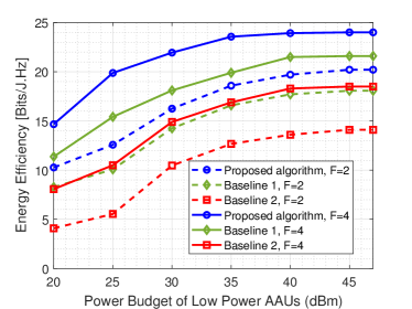
Figure 2: EE versus the value of power budget for each AAU for different number of AAUs.

All the above scenarios are investigated under different system parameters which are discussed in the following. First, we investigate the effect of variation of power budget on the EE of the network for different number of AAUs in Fig. 2. In this figure, we change the power budget values from $20$ dBm to $47$ dBm and also we observe that the EE first increases and then is saturated when the transmit power is larger than $35$ dBm, i.e., $P_{\max}^{f}=35$ dBm. This is because of exploiting power control via designing beamforming for all schemes, and also we can deduct that the beamforming works well to improve EE up to the maximum point. Besides, we observe that the performance of our proposed SIC ordering and beamforming algorithm in terms of EE significantly outperforms the other baselines. The main reason behind this achievement is that the proposed SIC ordering algorithm is performed via optimizing the SIC ordering variable which is exploited to handle the intra-cell and inter-cell interference to maximize EE. We also observe that our proposed algorithm has a better performance as compared to baseline 1 due to performing resource allocation design and SIC ordering jointly in a one-step optimization problem. While, in baseline 2, SIC ordering is based on the absolute value of the channel gains. However, SIC ordering in baseline 2 is applicable with an acceptable performance guarantee for single antenna systems and cannot be applied for MISO NOMA systems, efficiently. Also, this figure investigates the effect of AAUs on the EE of the system. It is evident that our proposed algorithm outperforms other baseline schemes due to performing joint user association and subcarrier allocation which improves significantly the performance of the system.

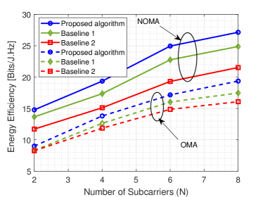
Figure 3: EE versus the number of shared subcarriers in each AAU for NOMA and OMA.

In Fig. 3, we study the effect of the number of subcarriers and also the performance of NOMA as compared to the conventional OMA on the baseline schemes. It is observed that the improvement of the proposed algorithm compared to the baselines is sustainable. This improvement is achieved not only in the NOMA-based systems but also in the OMA-based systems. Note that in OMA, there is no intra-cell inference due to orthogonality in the utilization of the subcarriers. Besides, our proposed SIC ordering controls the inter-cell interference. Thus, our designed SIC ordering and beamforming are applicable not only for NOMA but also for any co-channel interference suffered communication networks without any need on the CSI of these channels. Consequently, the improvement of EE in NOMA is more than OMA. Also we can conclude that the performance of NOMA is much better than that of OMA due to exploiting each subcarrier more than one in the network.

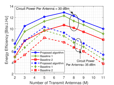
Figure 4: Energy efficiency versus the of number of antennas in each AAU.

In Fig. 4, we evaluate the EE of the considered schemes while considering the effect of the number of antennas in each AAU for different circuit power values. As can be seen from this figure, EE increases as the number of antennas increases due to the array giants and spatial diversity, and then drops after certain value for the number of antennas, i.e., $M>7$. This is because that employing more antenna enables high degrees of freedom in the spatial diversity gain which turns on improving SE while exceeding power consumption, specifically hardware power consumption which linearly increases as $M$ increases due to activating RF chain per each antenna. While the SE is changed slowly with respect to the value of $M$ which turns a strike a balance between SE and power consumption which leads to trade-off between SE and EE. Further, for the higher values of circuit power, the maximum value of EE is obtained for a lower number of $M$. This is because that system’s aggregated power consumption has a greater impact on improving system’s EE than maximizing the SE as SE commensurates to log-function. The interesting results from this evaluation can be explained as two folds: First, we need an appropriate beamforming design for massive antennas communication systems and second there is a need for designing an efficient antenna selection algorithm to select appropriate antennas and then doing precoding, especially for massive MIMO mmWave 6G networks. Also, this figure reveals the performance of our SIC ordering algorithm for massive antennas networks. In our future work, we will propose an appropriate antenna selection (finding optimum $M$) as well as beamforming design for massive mmWave networks.

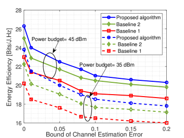
Figure 5: Impact of channel estimation error bound on the EE.

Fig. 5 illustrates the impact of channel estimation error on the EE for different values of the power budget. As can be seen, the relation between the error bound and the system EE is indirect. Also, the upper bound is obtained for the perfect CSI setting. It is seen that with increasing the error bound, our algorithm has a vigorous capability for deducting the impact of the imperfect CSI. It can be also observe that the performance gap with respect to the baseline schemes becomes significantly large. This is because of the existing indirect efficacy of the error bound on the performance of the SIC ordering based on the channel gains. It is worthwhile to note that performing SIC based on the channel gains needs full CSI which is not practical in the real wireless communication networks. Furthermore, more power consumption is needed for large values of the error bound to reach the same SE which makes the reduction on EE with increasing the error bound. In other words, for a fixed value of consumed power, the SE tends to low values for the higher error bounds which results in the EE reduction.

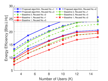
Figure 6: EE versus the number of users for different reused numbers.

Moreover, we study the behavior of EE achieved via the scenarios with respect to the number of users and maximum reuse number of each subcarrier in each AAU which is plotted in Fig. 6. Note that when the reuse number is $1$, the considered network operates as OMA while for values of $2$ and $3$, the network operates as NOMA. From this figure, it can be observed that the EE grows with the number of users and reuse factor of NOMA because of multi user diversity. In addition, for the higher number of reuse factors in NOMA, the improvement on the EE is low. The reason behind this trend is that the high reuse factors in NOMA boosts the denominator of the system throughput due to incorporating intra-cell interference in the data rate which results in an exceeding power consumption and consequently degrading the EE of the system. Furthermore, we can declare that for the high reuse factor, it is better to adopt clustering, i.e., user pairing methods, especially for the large number of users (e.g., massive connections).

Finally, we investigate the performance gap between the exactly robust solution denoted by ExRS (approach in Remark 1) and strictly bounded robust solution denoted by SBRS, and the behavior of the introduced penalty function in (III-A). For the First, Fig. 7 shows the performance comparison between ExRS and SBRS under variation of channel estimation error bound for different power budget for macro AAU denoted by $P_{\max}^{1}$. As can be seen from the figure, for low power budget and small values of the error approximately the performance of ExRS and SBRS are close to each other.

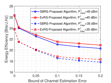
Figure 7: EE versus the channel estimation error bound for different robust algorithms.

Moreover, the effect of penalty factors on the penalty function is examined in Fig. 8. In this figure, $P_{\max}^{1}=35\leavevmode\nobreak\ \text{dBm},\leavevmode\nobreak\ K=8,\leavevmode\nobreak\ N=5$, $\lambda=\mu$, and both axes are plotted in the Logarithmic scale. Note that in “Without Round’, the penalty function values is the penalty function in (III-A) (“Term 1+Term 2”), and in “With Round”, the penalty function is only the penalty term for the rank-one (“Term 2” in (III-A)) due to $h(\bm{\xi},\bm{\rho},\mathbb{x},\lambda)=0$. As can be seen form Fig. 8, the penalty function values close to $0$, for the sufficiently large value of penalty factors, e.g., $10^{5}$, which ensures achieving a rank-one solution and the relaxed binary variables converges to binary ones.

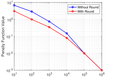
Figure 8: Impact of penalty factors on the penalty function of (III-A).

V Conclusion Remarks

In this paper, we proposed a novel SIC ordering and also provided a robust and efficient algorithm for resource allocation and beamforming design for C-RAN assisted MC NOMA networks with imperfect CSI. In particular, we formulated the worst-case EE by optimizing the SIC ordering, beamforming, and scheduling variables. Although, the underlying optimization problem is non-convex which is in the form of MINLP, we adopted majarization-minimization and penalty factor methods to convert it into the convex one. Furthermore, we provided a low complexity algorithm based on two-step iterative solution to strike the balance between the complexity and performance gain. Extensive simulations were provided to assess the performance of the proposed algorithms. Moreover, simulation results unveil the superiority of the proposed algorithm as compared to the baseline schemes.
The SIC ordering algorithm in NOMA-based communications has not been well addressed, especially restraining the inter-cell interference, and it would be a critical issue and pivotal impact on the performance of co-channel interference communication networks. In order to broaden a new horizon that is inferred from the results for the future of massive antennas and high energy efficiency that necessitates the ubiquitous 6G, it is crucial to design efficient antenna selection, clustered beamforming, channel estimation, and spectrum management algorithms in a future wireless networks.

VI Appendix

VI-A Proof of Proposition 1

The proof includes two parts: 1) minimization and 2) maximization which are discussed as follows.
Proof of minimization: Using an arbitrary positive multiplier $\phi\geq 0$, the Lagrangian function of (19) can be written as

$$\mathcal{L}(\bm{\Delta}_{k,n,f},\phi)=\text{Tr}[(\tilde{\mathbb{H}}_{k,n,f}+\bm{\Delta}_{k,n,f})\mathbb{W}_{k,n,f}]$$

$$+\phi(\text{Tr}\leavevmode\nobreak\ [\bm{\Delta}_{k,n,f}\bm{\Delta}_{k,n,f}^{\dagger}]-e_{k,n,f}).$$ (82)

Setting the derivative of the Lagrangian with respect to $\bm{\Delta}_{k,n,f}$ to zero, we have:

$$\nabla_{\bm{\Delta}^{*}_{k,n,f}}\mathcal{L}(\bm{\Delta}_{k,n,f},\phi)=\mathbb{W}^{\dagger}_{k,n,f}+\phi\bm{\Delta}_{k,n,f}=0.$$ (83)

The optimal value of $\bm{\Delta}_{k,n,f}$ is denoted by $\bm{\Delta}^{*}_{k,n,f}$ which can be obtained as $\bm{\Delta}^{*}_{k,n,f}=-\frac{1}{\phi}\mathbb{W}^{\dagger}_{k,n,f}.$ We also differentiate the Lagrangian function with respect to $\phi$ and equates it to zero as $\nabla_{\phi}\mathcal{L}(\bm{\Delta}_{k,n,f},\phi)=0,$ where the optimal solution for $\phi$ is given by $\phi^{*}=\frac{1}{e_{k,n,f}}\|\mathbb{W}^{\dagger}_{k,n,f}\|.$ By substituting the optimal value of $\phi$, i.e., $\phi^{*}$, we conclude that

$$\bm{\Delta}^{f,\text{min}}_{k,n}=-e_{k,n,f}\frac{\mathbb{W}^{\dagger}_{k,n,f}}{\|\mathbb{W}^{\dagger}_{k,n,f}\|}.$$ (84)

Hessian of the Lagrangian function verifies the obtained solution is minimum. To this end, we need to check the second derivative at the optimal point that should be positive semi-definite, i.e., [54]

$$\nabla^{2}_{\bm{\Delta}_{k,n,f}}\mathcal{L}(\bm{\Delta}_{k,n,f}^{*},\phi^{*})=$$ (85)

$$\frac{\|\mathbb{W}^{\dagger}_{k,n,f}\|}{e_{k,n,f}}\bigg{(}\text{vec}\{\mathbb{I}_{M}\}\text{vec}\{\mathbb{I}_{M}\}\bigg{)}^{T}\succeq\mathbb{0}.$$ (86)

Proof of maximization: The Lagrangian of (20) is given by

$$\mathcal{L}(\bm{\Delta}_{k,n,f^{\prime}},\phi)=\text{Tr}[(\tilde{\mathbb{H}}_{k,n,f^{\prime}}+\bm{\Delta}_{k,n,f^{\prime}})\mathbb{W}_{i,n,f^{\prime}}]$$

$$-\phi(\text{Tr}\leavevmode\nobreak\ [\bm{\Delta}_{k,n,f^{\prime}}\bm{\Delta}_{k,n,f^{\prime}}^{\dagger}]-e^{2}_{k,n,f^{\prime}}).$$ (87)

By differentiating above function with respect to $\bm{\Delta}_{k,n,f^{\prime}}$ and setting the derivative to zero, we have:

$$\nabla_{\bm{\Delta}^{*}_{k,n,f^{\prime}}}\mathcal{L}(\bm{\Delta}_{k,n,f^{\prime}},\phi)=\mathbb{W}^{\dagger}_{i,n,f^{\prime}}-\phi\bm{\Delta}_{k,n,f^{\prime}}=0.$$ (88)

We will found that $\bm{\Delta}^{*}_{k,n,f^{\prime}}=\frac{1}{\phi}\mathbb{W}^{\dagger}_{i,n,f^{\prime}}.$ Following the same steps for eliminating the role of $\phi$, we obtain that

$$\bm{\Delta}^{f^{\prime},\text{max}}_{k,n}=e_{k,n,f^{\prime}}\frac{\mathbb{W}^{\dagger}_{i,n,f^{\prime}}}{\|\mathbb{W}^{\dagger}_{i,n,f^{\prime}}\|}.$$ (89)

Hessian of the Lagrangian function verifies that the obtained solution is maximum. Hence, we check the second derivative at the optimal point that should be negative semi-definite, i.e., [54]

$$\nabla^{2}_{\bm{\Delta}_{k,n,f}}\mathcal{L}(\bm{\Delta}_{k,n,f}^{*},\phi^{*})=$$

$$-\frac{\|\mathbb{W}^{\dagger}_{k,n,f}\|}{e_{k,n,f}}\bigg{(}\text{vec}\{\mathbb{I}_{M}\}\text{vec}\{\mathbb{I}_{M}\}\bigg{)}^{T}\preceq\mathbb{0}.$$ (90)

VI-B Proof of Proposition 2

We aim to prove this proposition by using the abstract Lagrangian duality. The primal problem of (35) can be written as $p^{*}=\max_{\mathbb{W},\bm{\xi},\bm{\rho},\mathbb{x}}\min_{\lambda}\mathcal{L}(\mathbb{W},\bm{\xi},\bm{\rho},\mathbb{x}),$ where the dual problem of (49a) is given by:

$$d^{*}=\min_{\lambda}\max_{\mathbb{W},\bm{\xi},\bm{\rho},\mathbb{x}}\mathcal{L}(\mathbb{W},\bm{\xi},\bm{\rho},\mathbb{x}).$$ (91)

For simplicity, we also define:

$$\mu(\lambda)\triangleq\max_{\mathbb{W},\bm{\xi},\bm{\rho},\mathbb{x}}\mathcal{L}(\mathbb{W},\bm{\xi},\bm{\rho},\mathbb{x}).$$ (92)

Based on the weak duality theorem, we have:

$$p^{*}\leq d^{*}=\min_{\lambda\geq 0}\mu(\lambda).$$ (93)

It should be noted that for the feasible set, we have 2 cases as follows:
Case 1: One can easily verify that at the optimal point, we have

$$\mathcal{R}_{1}:\sum_{i,k\in\mathcal{K}}\sum_{n\in\mathcal{N}}\bigg{(}\xi_{i,n}^{k}-(\xi_{i,n}^{k})^{2}\bigg{)}=0,\leavevmode\nobreak\$$ (94)

$$\mathcal{R}_{2}:\sum_{f\in\mathcal{F}}\sum_{k\in\mathcal{K}}\sum_{n\in\mathcal{N}}\bigg{(}\rho_{k,n}^{f}-(\rho_{k,n}^{f})^{2}\bigg{)}=0,$$ (95)

$$\leavevmode\nobreak\ \mathcal{R}_{3}:\leavevmode\nobreak\ \sum_{f\in\mathcal{F}}\sum_{i,k\in\mathcal{K}}\sum_{n\in\mathcal{N}}\bigg{(}x_{i,n}^{k,f}-(x_{i,n}^{k,f})^{2}\bigg{)}=0.$$ (96)

As a result, $d^{*}$ is also a feasible solution of (35). Subsequently, substituting the optimal value of $\lambda$, i.e., $\lambda^{*}$, into the optimization problem (35) yields

$$d^{*}=\mu(\lambda^{*})=\max_{\mathbb{W},\bm{\xi},\bm{\rho},\mathbb{x}}\mathcal{L}(\mathbb{W},\bm{\xi},\bm{\rho},\mathbb{x})=p^{*}.$$ (97)

Moreover, referring to Lagrangian function, in the region $\bm{\xi},\bm{\rho},\leavevmode\nobreak\ \mathbb{x},\leavevmode\nobreak\ \mathcal{R}_{1},\leavevmode\nobreak\ \mathcal{R}_{2},\leavevmode\nobreak\ \mathcal{R}_{3}$, function $\mu(\lambda)$ is a monotonically decreasing function with respect to $\lambda$. On the other hand, it is argued that $d^{*}=\min_{\lambda\geq 0}\mu(\lambda)$, so we have

$$\mu(\lambda)=d^{*},\forall\leavevmode\nobreak\ \lambda\geq\lambda^{*}.$$ (98)

This means that for any value of $\lambda\geq\lambda^{*}$, the solution of Lagrangian function yields the optimal solution of (35).
Case 2: The second case occurs when some of integer variables take some values between 0 and 1, causing

$$\mathcal{R}_{1}>0,\leavevmode\nobreak\ \mathcal{R}_{2}>0,\leavevmode\nobreak\ \mathcal{R}_{3}>0.$$ (99)

Referring to the Lagrangian function and (92), at the optimal point, $\mu(\lambda^{*})$ tends to $-\infty$. However, this can not happen as it contradicts with primal solution stating that $\mu(\lambda^{*})$ is limited from below by the solution of (35) which is always greater than zero. Thus, at the optimal point, we have, $\mathcal{R}_{1}=0,\leavevmode\nobreak\ \mathcal{R}_{2}=0$, and $\mathcal{R}_{3}=0$.

References

• [1] W. Saad, M. Bennis, and M. Chen, “A vision of 6G wireless systems: Applications, trends, technologies, and open research problems”, IEEE Network. vol. 34, no. 3, pp. 134-142, May. 2020.
• [2] A. Zakeri et al., “Digital transformation via 5G: Deployment plans,” in Proc. ITU Kaleidoscope: Industry-Driven Digital Transformation (ITU K), Ha Noi, Vietnam, 2020, pp. 1-8.
• [3] C. Pan, M. Elkashlan, J. Wang, J. Yuan and L. Hanzo, “User-centric C-RAN architecture for ultra-dense 5G networks: Challenges and methodologies,” IEEE Commun. Mag., vol. 56, no. 6, pp. 14-20, Jun. 2018.
• [4] Z. Ding, L. Dai, R. Schober, and H. Vincent Poor, “NOMA meets finite resolution analog beamforming in massive MIMO and millimeter-wave networks,” IEEE Commun. Lett., vol. 21, no. 8, pp. 1879-1882, Aug. 2017.
• [5] Z. Ding, X. Lei, G. K. Karagiannidis, R. Schober, J. Yuan, and V. K. Bhargava, “A survey on non-orthogonal multiple access for 5G networks: research challenges and future trends,” IEEE J. Select. Areas Commun., vol. 35, no. 10, pp. 2181-2195, Oct. 2017.
• [6] Z. Ding, P. Fan, and H. V. Poor, “Impact of user pairing on 5G non-orthogonal multiple-access downlink transmissions,” IEEE Trans. Veh. Technol., vol. 65, no. 8, pp. 6010-6023, Aug. 2016.
• [7] Z. Ding, Z. Yang, P. Fan, and H. V. Poor, “On the performance of non-orthogonal multiple access in 5G systems with randomly deployed users,” IEEE Signal Process. Lett., vol. 21, no. 12, pp. 1501-1505, Dec. 2014.
• [8] K. Yang, N. Yang, N. Ye, M. Jia, Z. Gao, and R. Fan, “Non-orthogonal multiple access: Achieving sustainable future radio access,” IEEE Commun. Mag., vol. 57, no. 2, pp. 116–121, Nov. 2019.
• [9] L. Dai, B. Wang, Z. Ding, Z. Wang, S. Chen, and L. Hanzo, “A survey of non-orthogonal multiple access for 5G,” IEEE Commun. Surveys Tuts., vol. 20, no. 3, pp. 2294-2323, May. 2018.
• [10] S. M. R. Islam, M. Zeng, O. A. Dobre, and K. Kwak, “Resource allocation for downlink NOMA systems: Key techniques and open issues,” IEEE Wireless Commun., vol. 25, no. 2, pp. 40-47, Apr. 2018.
• [11] Z. Ding, R. Schober, and H. V. Poor, “Unveiling the importance of SIC in NOMA systems—Part 1: State of the art and recent findings,” IEEE Commun. Lett., vol. 24, no. 11, pp. 2373-2377, Nov. 2020.
• [12] Z. Ding, R. Schober, and H.V. Poor, “Unveiling the importance of SIC in NOMA systems: Part II: New results and future directions,” IEEE Commun. Lett., vol. 24, no. 11, pp. 2378-2382, Nov. 2020.
• [13] M. F. Hanif, Z. Ding, T. Ratnarajah, and G. K. Karagiannidis, “A minorization-maximization method for optimizing sum rate in the downlink of non-orthogonal multiple access systems,” IEEE Trans. Signal Process., vol. 64, no. 1, pp. 76–88, Jan. 2016.
• [14] Y. Sun, D. W. K. Ng, Z. Ding, and R. Schober, “Optimal joint power and subcarrier allocation for full-duplex multicarrier non-orthogonal multiple access systems,” IEEE Trans. Commun., vol. 65, no. 3, pp. 1077-1091, Mar. 2017.
• [15] Z. Wei, D. W. K. Ng, J. Yuan, and H. M. Wang, “Optimal resource allocation for power-efficient MC-NOMA with imperfect channel state information,” IEEE Trans. Commun., vol. 65, no. 9, pp. 3944-3961, Sep. 2017.
• [16] S. Sharma, K. Deka, V. Bhatia, and A. Gupta, “Joint power-domain and SCMA-based NOMA system for downlink in 5G and beyond,” IEEE Commun. Lett., pp. 1–1, Apr. 2019.
• [17] S. Li, M. Derakhshani and S. Lambotharan, “Outage-constrained robust power allocation for downlink MC-NOMA with imperfect SIC,” Proc. IEEE ICC, Kansas City, MO, USA, May. 2018, pp. 1-7.
• [18] M. Moltafet, P. Azmi, N. Mokari, M. R. Javan, and A. Mokdad, “Optimal and fair energy efficient resource allocation for energy harvesting-enabled-PD-NOMA-based HetNets,” IEEE Trans. Wireless Commun., vol. 17, no. 3, pp. 2054-2067, Mar. 2018.
• [19] Q. Zhang, Q. Li, and J. Qin, “Robust beamforming for non-orthogonal multiple-access systems in MISO channels,” IEEE Trans. Veh. Technol, vol. 65, no. 12, pp. 10231-10236, Dec. 2016.
• [20] Y. Sun, D. W. K. Ng, and R. Schober, “Optimal resource allocation for multicarrier MISO-NOMA systems,” Proc. IEEE ICC,, Paris, France, May. 2017, pp. 1-7.
• [21] A. Zakeri, M. Moltafet, and N. Mokari, “Joint radio resource allocation and SIC ordering in NOMA-based networks using submodularity and matching theory,” IEEE Trans. Veh. Technol., vol. 68, no. 10, pp. 9761-9773, Oct. 2019.
• [22] H. Al-Obiedollah, K. Cumanan, J. Thiyagalingam, A. G. Burr, Z. Ding and O. A. Dobre, “Energy efficiency fairness beamforming designs for MISO NOMA systems,” Proc. IEEE WCNC,, Marrakesh, Morocco, Morocco, Apr. 2019, pp. 1-6.
• [23] Y. Zhang, H. M. Wang, T. X. Zheng, and Q. Yang, “Energy-efficient transmission design in non-orthogonal multiple access,” IEEE Trans. Veh. Technol, vol. 66, no. 3, pp. 2852–2857, Mar. 2017.
• [24] F. Fang, H. Zhang, J. Cheng, and V. C. M. Leung, “Energy-efficient resource allocation for downlink non-orthogonal multiple access network,” IEEE Trans. Commun., vol. 64, no. 9, pp. 3722–3732, Sep. 2016.
• [25] F. Alavi, K. Cumanan, Z. Ding, and A. G. Burr, “Robust beamforming techniques for non-orthogonal multiple access systems with bounded channel uncertainties,” IEEE Commun. Lett., vol. 21, no. 9, pp. 2033–2036, Sep. 2017.
• [26] F. Fang, H. Zhang, J. Cheng, S. Roy, and V. C. M. Leung, “Joint user scheduling and power allocation optimization for energy-efficient NOMA systems with imperfect CSI,” IEEE J. Select. Areas Commun., vol. 35, no. 12, pp. 2874–2885, Dec. 2017.
• [27] F. Alavi, K. Cumanan, M. Fozooni, Z. Ding, S. Lambotharan, and O. A. Dobre, “Robust energy-efficient design for MISO non-orthogonal multiple access systems,” IEEE Trans. Commun., vol. 67, no. 11, pp. 7937-7949, Nov. 2019.
• [28] M. S. Ali, E. Hossain, A. Al-Dweik, and D. I. Kim, “Downlink power allocation for CoMP-NOMA in multi-cell networks,” IEEE Trans. Commun., vol. 66, no. 9, pp. 3982–3998, Sep. 2018.
• [29] K. Wang, Y. Liu, Z. Ding, A. Nallanathan, and M. Peng, “User association and power allocation for multi-cell non-orthogonal multiple access networks,” IEEE Trans. Wireless Commun., vol. 18, no. 11, pp. 5284-5298, Nov. 2019.
• [30] A. Wolf, P. Schulz, M. Dörpinghaus, J. C. S. Santos Filho, and G. Fettweis, “How reliable and capable is multi-connectivity?,” IEEE Trans. Commun., vol. 67, no. 2, pp. 1506-1520, Feb. 2019.
• [31] D. W. K. Ng, E. S. Lo, and R. Schober, “Energy-efficient resource allocation in multi-cell OFDMA systems with limited backhaul capacity,” IEEE Trans. Wireless Commun., vol. 11, no. 10, pp. 3618-3631, Oct. 2012.
• [32] A. Zakeri, N. Mokari, and H. Yanikomeroglu, “Joint radio resource allocation and 3D beam-forming in MISO-NOMA-based network with profit maximization for mobile virtual network operators.” arXiv preprint arXiv:1907.05161 (2019).
• [33] A. Khalili, M. R. Mili, M. Rasti, S. Parsaeefard, and D. W. K. Ng, “Antenna selection strategy for EE maximization in uplink OFDMA networks: A multi-objective approach,” IEEE Trans. Wireless Commun., vol. 19, no. 1, pp. 595-609, Jan. 2020.
• [34] A. Khalili, S. Zarandi, and M. Rasti, “Joint resource allocation and offloading decision in mobile edge computing,” IEEE Commun. Lett., vol. 23, no. 4, pp. 684-687, Apr. 2019.
• [35] A. Zappone, E. Björnson, L. Sanguinetti, and E. Jorswieck, “Globally optimal energy-efficient power control and receiver design in wireless networks,” IEEE Trans. Signal Process., vol. 65, no. 11, pp. 2844-2859, 1 Jun. 2017.
• [36] V. W. S. Wong, R. Schober, D. W. K. Ng, and L. C. Wang, Key technologies for 5G wireless systems, 1st ed. Cambridge University Pres, 2017.
• [37] A. Khalili, S. Akhlaghi, H. Tabassum, and D. W. K. Ng, “Joint user association and resource allocation in the uplink of heterogeneous networks,” IEEE Wireless Commun. Lett., vol. 9, no. 6, pp. 804-808, Jun. 2020.
• [38] Y. Wang, L. Ma, and Y. Xu, “Joint network optimization in cooperative transmission networks with imperfect CSI,” Proc. IEEE ICC, Kuala Lumpur, Malaysia, May. 2016, pp. 1-6.
• [39] J. Lee and S. Leyffer, Mixed integer nonlinear programming. Springer Science Business Media, 2011.
• [40] L. Sboui, Z. Rezki, A. Sultan, and M. Alouini, “A new relation between energy efficiency and spectral efficiency in wireless communications systems,” IEEE Trans. Wireless Commun., vol. 26, no. 3, pp. 168-174, Jun. 2019.
• [41] M. Moltafet, S. Parsaeefard, M. R. Javan, and N. Mokari, “Robust radio resource allocation in MISO-SCMA assisted C-RAN in 5G networks,” IEEE Trans. Veh. Technol., vol. 68, no. 6, pp. 5758-5768, Jun. 2019.
• [42] M. Youssef, J. Farah, C. A. Nour, and C. Douillard, “Resource allocation in NOMA systems for centralized and distributed antennas with mixed traffic using matching theory,” IEEE Trans. Commun., vol. 68, no. 1, pp. 414-428, Jan. 2020.
• [43] T. Hoessler, P. Schulz, E. A. Jorswieck, M. Simsek, and G. P. Fettweis, “Stable matching for wireless URLLC in multi-cellular, multi-user systems,” IEEE Trans. Commun., vol. 68, no. 8, pp. 5228-5241, Aug. 2020.
• [44] Y. Saito, Y. Kishiyama, A. Benjebbour, T. Nakamura, A. Li, and K. Higuchi, “Non-orthogonal multiple Access (NOMA) for cellular future radio access,” Proc. IEEE VTC Spring, Dresden, Germany, Jun. 2013, pp. 1-5.
• [45] L. Salaün, M. Coupechoux, and C. S. Chen, “Joint subcarrier and power allocation in NOMA: Optimal and approximate algorithms,” IEEE Trans. on Signal Process., vol. 68, pp. 2215-2230, 2020.
• [46] Q. Zhang, Q. Li, and J. Qin, “Robust beamforming for non-orthogonal multiple-access systems in MISO channels,” IEEE Trans. Veh. Technol., vol. 65, no. 12, pp. 10231-10236, Dec. 2016.
• [47] C. Chao, C. Wang, C. Lee, H. Wei, and W. Chen, “Pair auction and matching for resource allocation in full-duplex cellular systems,” IEEE Trans. Veh. Technol., vol. 69, no. 4, pp. 4325-4339, Apr. 2020.
• [48] Q. Qi, X. Chen, and D. W. K. Ng, “Robust beamforming for NOMA-based cellular massive IoT with SWIPT,” IEEE Trans. Signal Process., vol. 68, pp. 211-224, 2020.
• [49] E. A. Gharavol, Y. Liang, and K. Mouthaan, “Robust downlink beamforming in multiuser MISO cognitive radio networks with imperfect channel-state information,” IEEE Trans. Veh. Technol., vol. 59, no. 6, pp. 2852-2860, Jul., 2010.
• [50] R. A. Addad, T. Taleb, M. Bagaa, D. L. C. Dutra, and H. Flinck, “Towards modeling cross-domain network slices for 5G,” in Proc. IEEE Global Communications Conference (GLOBECOM), Abu Dhabi, United Arab Emirates, Dec. 2018, pp. 1-7.
• [51] Glover, Fred. “Improved linear integer programming formulations of nonlinear integer problems.” Management Science, vol. 22, no. 4, pp. 455-460, 1975.
• [52] A. Ben-Tal and A. Nemirovski, “On polyhedral approximations of the second-order cone,” Math. Operations Res., vol. 26, no. 2, pp. 193–205, May 2001.
• [53] Z. Lin, M. Lin, J. Wang, T. de Cola, and J. Wang, “Joint beamforming and power allocation for satellite-terrestrial integrated networks with non-orthogonal multiple access,” in IEEE J. Sel. Topics Signal Process., vol. 13, no. 3, pp. 657-670, Jun. 2019.
• [54] A. Hjorungnes and D. Gesbert, “Complex-valued matrix differentiation: Techniques and key results,” in IEEE Trans. Signal Process., vol. 55, no. 6, pp. 2740-2746, Jun. 2007.
• [55] Chinneck, John W, “Feasibility and Infeasibility in Optimization: Algorithms and Computational Methods,” Springer Science & Business Media, vol. 118, 2007.