MPC-MPNet: Model-Predictive Motion Planning Networks for Fast, Near-Optimal Planning under Kinodynamic Constraints

Abstract

Kinodynamic Motion Planning (KMP) is to find a robot motion subject to concurrent kinematics and dynamics constraints. To date, quite a few methods solve KMP problems and those that exist struggle to find near-optimal solutions and exhibit high computational complexity as the planning space dimensionality increases. To address these challenges, we present a scalable, imitation learning-based, Model-Predictive Motion Planning Networks framework that quickly finds near-optimal path solutions with worst-case theoretical guarantees under kinodynamic constraints for practical underactuated systems. Our framework introduces two algorithms built on a neural generator, discriminator, and a parallelizable Model Predictive Controller (MPC). The generator outputs various informed states towards the given target, and the discriminator selects the best possible subset from them for the extension. The MPC locally connects the selected informed states while satisfying the given constraints leading to feasible, near-optimal solutions. We evaluate our algorithms on a range of cluttered, kinodynamically constrained, and underactuated planning problems with results indicating significant improvements in computation times, path qualities, and success rates over existing methods.

I INTRODUCTION

The motion planning problem is to find a path connecting the given start and goal states while satisfying all the desired constraints on the robot motion. Geometric motion planning is a simple instance that considers only collision-avoidance constraints with states representing the robot’s kinematics variables (e.g., position, joint-angles) [1]. However, in KMP, the state comprises position, velocity, and sometimes acceleration, and the robot motions are required to satisfy both kinematic (e.g., collision-avoidance) and dynamics (e.g., velocity and acceleration) constraints, which makes the problem PSPACE-hard and computationally demanding [1].

The KMP has a broad range of applications from torque-constrained robot manipulation to speed racing [2] and performing acrobatic motions [3]. The existing state-of-the-art methods solve KMP through Sampling-based Motion Planners (SMPs) [1] by constructing a tree that originates from a start state and expands by searching the entire state-space to reach the given goal state. The edges of the tree, connecting any two intermediate states, are formed by a local steering function. The local steering often requires solving a boundary-value problem (BVP) through trajectory optimization, which is known to be NP-hard [4] and fails when the boundary constraints are not satisfied. A recent development led to another sampling-based KMP approach [5], called Stable Sparse-RRT (SST), that circumvents solving BVPs by using a random shooting method for steering and achieves asymptotic optimality. However, it still takes long computation times from tens of seconds to minutes as environments become more complicated due to uniform exploration of state and control spaces.

In this paper, we propose an imitation learning-based approach named Model-Predictive Motion Planning Networks (MPC-MPNet). It has a deep neural networks-based generator and discriminator, which, once trained using expert data, outputs feasible paths that satisfy the given kinodynamic constraints. Our approach extends the Motion Planning Networks (MPNet) [6] and leverages collision-aware Model Predictive Control (MPC) methods in the planning loop for parallelizable local steering. Note that the original MPNet framework [6] considered only geometric planning problems and relied on bidirectional path expansions and re-planning steps for finding path solutions to given problems. In KMP, the bidirectional path extensions and re-planning steps to repair in-collision path segments often lead to discontinuity and infeasible paths. Therefore, in MPC-MPNet, we propose novel planning algorithms that perform only forward path expansion and avoid re-planning by building a set of informed possible paths. We evaluate our approach in challenging under-actuated robotics problems in complex, cluttered environments. Our results show that MPC-MPNet outperforms state-of-the-art planning algorithms in computational speed and generalizes to unseen planning problems with high success rates.

II Related Work

Figure 1: MPC-MPNetPath In each iteration, the neural generator predicts a batch of next states from a given current and select a collision-free state with a minimum estimated cost for the tree expansion using MPC.

This section presents a brief overview of related work done in the past for solving KMP problems. KMP algorithms depend on the local steering function to satisfy the motion constraints between any two given states. The local steering methods are usually implemented either as (i) random shooting methods which uniformly samples control sequences [7][8][5], (ii) predefined motion primitives [9], or (iii) local trajectory optimization solvers [10][11][12][13].

Sampling random control sequences for shooting method has the advantage of worst-case theoretical guarantees. For instance, the SST approach [5] leverages random exploration of control and state spaces to provide the worst-case asymptotic completeness and optimality guarantees. However, these methods struggle in higher-dimensional and cluttered planning spaces since uniform exploration takes large computation times to determine a feasible path solution. In contrast, the motion primitives methods generate a local database of optimal controllers in their offline stage [9] and use them for steering under KMP algorithms. However, as the motion primitive set is finite, it usually does not capture the entire control space and lacks completeness guarantees.

The trajectory optimization methods formulate local steering as an optimization problem and iteratively solve them for computing action sequences connecting the given states. For instance, [14][12] locally linearize the system and obtain Linear Quadratic Regulators’ (LQR) parameters using optimization for steering. Tedrake et. el [13] extend LQR methods to construct a tree connecting states within stability regions defined by LQR funnels. However, these methods add a substantial computational burden when constructing trees and do not apply to online planning problems. In a similar vein, Xie et. el [10] formulated local steering as BVP and used optimization to find their solutions. These BVP solvers operate in conjunction with traditional SMPs [1] for finding solutions to KMP problems. However, their approach often collapse when the boundary constraints are not satisfied.

Another class of methods in KMP learn local controllers for steering through reinforcement and imitation learning. For instance, [15] uses reinforcement learning (RL) to acquire local policy for steering within SMP methods. Similarly, [16] [17] constructs high-level landmarks, which are later connected by local RL policies. However, these methods inherit RL limitations such as requiring exhaustive interactions with their environments for learning. In the imitation learning paradigm, [18] and [19] use expert demonstrations to learn local policies for connecting given states, but they still rely on classical planners to generate those state sequences.

Recent developments overcome the limitations of classical motion planning by incorporating learned planning distributions into their algorithms [6][20][21][22]. These learning-based planners quickly generate feasible motion sequences online for finding path solutions but mostly consider geometric planning problems. Among them, MPNet [6] [20] generates end-to-end paths by exploiting learned distributions in a bidirectional manner throughout its planning and replanning process. MPNet has also been extended to consider kinematic [23] and non-holonomic [24] constraints. However, these extensions still rely on bidirectional planning, which often leads to discontinuities and infeasible paths in KMP problems.

III Problem Definition

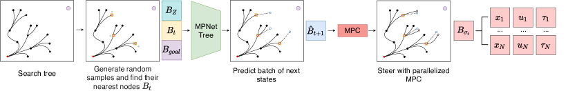
Figure 2: MPC-MPNetTree The neural generator predicts a batch of next states from nearest neighbors of random states inside the search tree. Our parallelized MPC finds the local controllers between randomly selected start and neurally generated next states for extending multiple branches of tree simultaneously towards the given goal state.

Let $\mathcal{C}$ denote a configuration space (C-space) of a mechanical system, where collision and collision-free regions are represented as $\mathcal{C}_{obs}$ and $\mathcal{C}_{free}=\mathcal{C}\backslash\mathcal{C}_{obs}$, respectively. Let $\mathcal{X}$ denote the state space in which a state, $\boldsymbol{x}=(\boldsymbol{c},\dot{\boldsymbol{c}})\in\mathcal{X}$, contains a configuration $\boldsymbol{c}\in\mathcal{C}$ and the time derivative $\dot{\boldsymbol{c}}$. Like C-space, the state space also contains the collision $\mathcal{X}_{obs}$ and collision-free $\mathcal{X}_{free}$ state spaces. The system’s dynamics model, represented by an implicit set of equations, can be formulated as $\dot{\boldsymbol{x}}={f}(\boldsymbol{x},\boldsymbol{u})$, where $\boldsymbol{u}$ denotes the control input to a system from a feasible control set $\mathcal{U}$. In general, the objective of KMP for the given initial state $\boldsymbol{x}_{init}$ and goal region $\mathcal{X}_{goal}\subset\mathcal{X}_{free}$ is to find a collision-free trajectory $\boldsymbol{\sigma}=[(\boldsymbol{x},\boldsymbol{u},\boldsymbol{\tau})_{t}]^{T}_{t=0}$, comprising a sequence of states $[\boldsymbol{x}_{t}]^{T}_{t=0}\mapsto\mathcal{X}_{free}$ and controls $[\boldsymbol{u}_{t}]^{T}_{t=0}\mapsto\mathcal{U}$ with their corresponding durations $[\boldsymbol{\tau}_{t}]^{T}_{t=0}$, such that $\boldsymbol{x}(0)=\boldsymbol{x}_{init}$, $\boldsymbol{x}(T)\in\mathcal{X}_{goal}$.

IV Model Predictive Motion Planning Networks

In this section, we present MPC-MPNet, an end-to-end learning-based KMP algorithm. MPC-MPNet iteratively generates waypoints and local steering trajectories to construct collision-free paths connecting the start and goal states. It includes a neural generator, discriminator, and two novel planning algorithms named MPC-MPNetPath and MPC-MPNetTree. The main components of our approach are described as follows.

Methods/networks Methods/mpc

Methods/parallelazion

Methods/planners

(a)

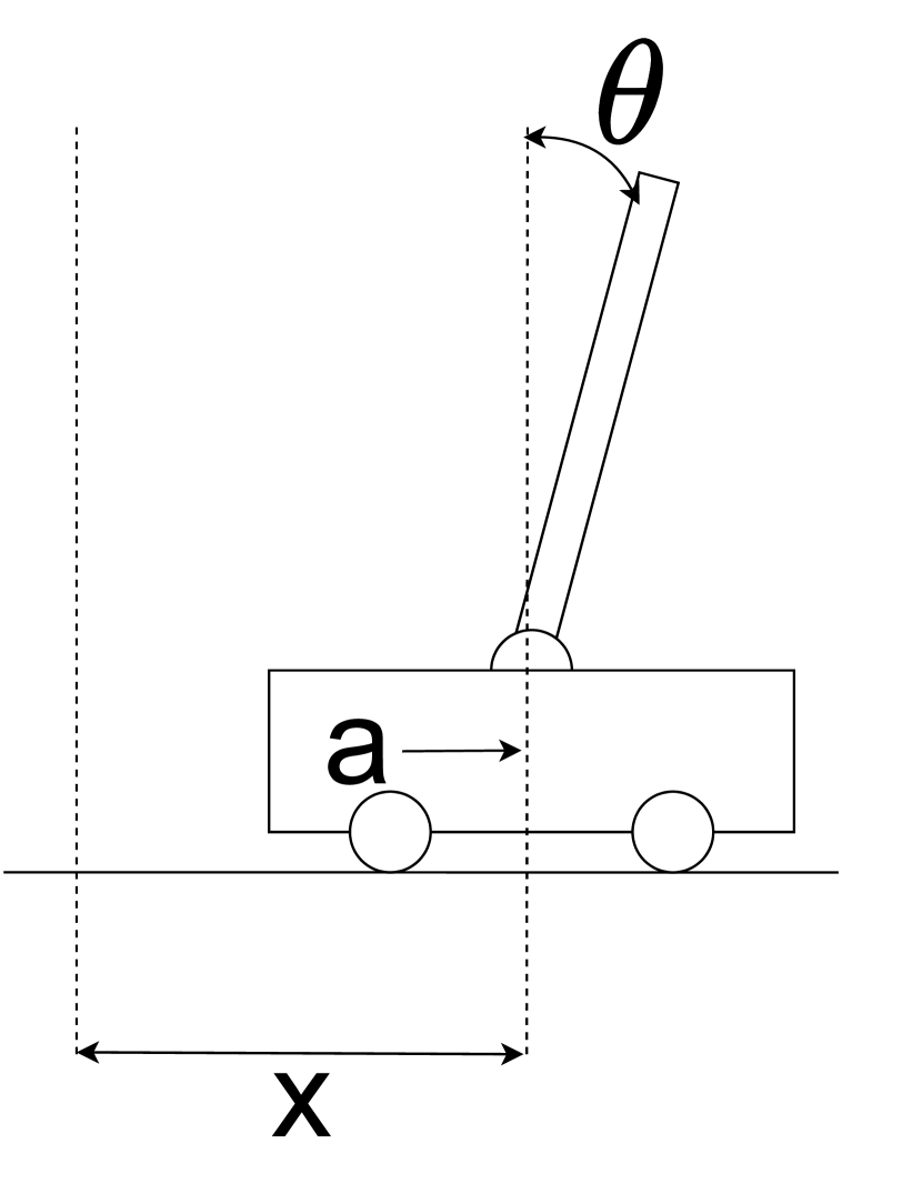
(b)

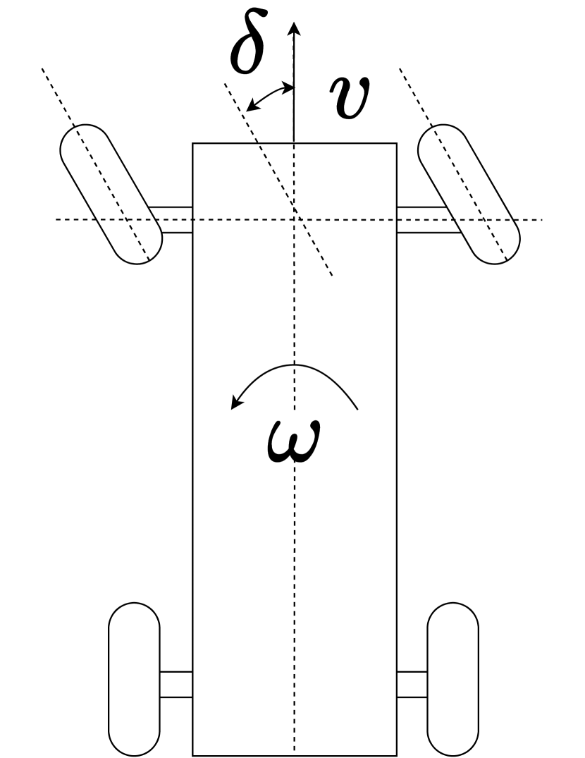
(c)

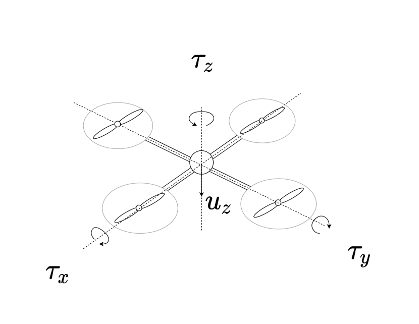
(d)

Figure 3: We consider the following robotic systems, (a) Acrobot, (b) Cartpole, (c) Car, and (d) Quadrotor, with complex dynamics for our cluttered, kinodynamically constrained environments.

V Implementation Details

Methods	Planning Tasks
	Acrobot	Cart-Pole	Quadrotor	Car-like
MP-Path	$5.09\pm 6.87$ $(9.88\pm 8.70)$	$4.74\pm 7.37$ $(7.93\pm 9.13)$	$\boldsymbol{0.46\pm 2.12}$ $(\boldsymbol{0.41\pm 1.12})$	$8.96\pm 12.33$ $(19.10\pm 21.25)$
MP-Tree	$\boldsymbol{4.19\pm 6.03}$ $(\boldsymbol{6.13\pm 7.90})$	$\boldsymbol{4.43\pm 6.07}$ $(\boldsymbol{4.36\pm 5.55})$	$2.26\pm 3.26$ ${(1.78\pm 2.45)}$	$\boldsymbol{7.51\pm 8.72}$ $(\boldsymbol{8.40\pm 11.48})$
SST	$28.32\pm 20.53$ $(21.37\pm 23.02)$	$14.99\pm 14.29$ $(12.21\pm 10.11)$	$143.69\pm 143.43$ $(251.03\pm 197.83)$	$41.69\pm 70.31$ $(28.16\pm 40.00)$

TABLE I: The total mean computation times with standard deviations in seen and unseen (reported inside parenthesis) test environments are presented for MPC-MPNetPath (MP-Path), MPC-MPNetTree (MP-Tree), and SST in various kinodynamic planning problems.

This section describes the necessary implementation details of our frameworks with their training and testing environments. We implement our neural modules using Pytorch and export them to C++ with Torchscript. Our parallelized MPC algorithm follows standard GPU programming. For the training and testing environments, we consider the following kinodynamically constrained, cluttered environments with schematics shown in Fig. 3.

V-1 Acrobot

We use the acrobot dynamics as specified in [30]. The state space is defined as $[\theta_{1},\theta_{2}.\dot{\theta_{1}},\dot{\theta_{2}}]\in[-\pi,\pi]^{2}\times[-6,6]^{2}$. The control space is defined as $[-4,4]$. We generate four rectangular obstacles and restrict the center of the obstacles to lie inside the annulus that affects the acrobot movement.

V-2 Cartpole

The cartpole dynamics are used as specified in [31]. The state space is defined as: $[x,\dot{x},\theta,\dot{\theta}]\in[-30,30]\times[-40,40]\times[-\pi,\pi]\times[-2,2]$. and the control space is defined as $[-300,300]$. We randomly place seven rectangular obstacles in the environment to challenge and restrict the cartpole motion.

V-3 Car

This is a 2D first-order car system, where the state space is of 3DOF, including position and orientation. The control inputs are the position velocity and angular velocity. The state space is defined as $[x,y,\theta]\in[-25,25]\times[-35,35]\times[-\pi,\pi]$ and control space bound as $[0,2]\times[-0.5,0.5]$. We randomly place five rectangular obstacles in the workspace, and limit the distance between obstacles to ensure narrow passages.

V-4 Quadrotor

We define the quadrotor dynamics as in [32]. The state space is defined as: $[p,q,\dot{p},{\omega}]$, where $p$ and $q$ denote the position and orientation of the quadrotor, respectively, with their corresponding time derivatives, indicating velocity, represented as $\dot{p}$ and $\omega$. The control space is 4 dimensional with bound $[-15,-5]\times[-1,1]^{3}$. We randomly place 10 obstacles in the workspace space and ensure the scene is cluttered.

In each of the cases mentioned above, we set up 10 environments by random placement of the obstacles, each with 1000-2000 randomly sampled start and goal state pairs. The $10-20\%$ of data is used for testing, and the remaining for the training. In our test dataset, we also include two unseen environments for each problem, created by random placement of obstacles. We ensure these environments to be different from the ten seen settings, and for each, we randomly sample 100-200 valid start and goal pairs for evaluation. Hence, in total, our test dataset contains 12 environments for the given setups. The demonstration trajectories for the training data are obtained using the SST algorithm. Furthermore, we obtain the point-cloud of the environments, by randomly sampling the obstacle space and processing them into voxel $\boldsymbol{v}$ of size $32\times 32\times 32$.

VI Results

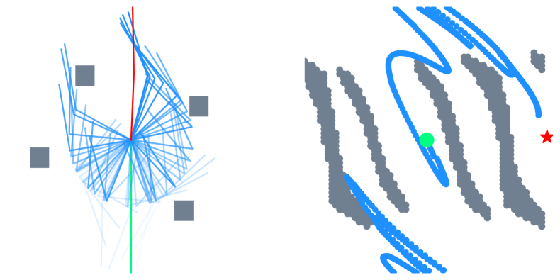
(a) MPC-MPNet: $t=5.5s$, $c=10.9$

(b) SST: $t=52.4s$, $c=11.2$

Figure 4: Acrobot environment: The workspace (left) and state-space (right) trajectories are shown in each subfigure. In this example, the start state is $[0,0,0,0]$, and goal states are randomly distributed around the vertical configuration. From the results, it can be seen that MPC-MPNet could generate a path of comparable lengths as SST with lesser amount of time.

We present a set of experiments to compare the computation time, path quality, and success rate of MPC-MPNetPath, MPC-MPNetTree, and SST planning algorithms. All experiments were performed on the same system with 32GB RAM, GeForce GTX 1080 GPU, and 3.40GHz$\times$8 Intel Core i7 processor.

VI-A Comparative Studies

This study compares the computation time, success rate, and path quality (measured by time-to-reach) of MPC-MPNetPath, MPC-MPNetTree, and SST algorithms in Cart-Pole, Acrobot, Car, and Quadrotor environments. All evaluation planning problems were unique and not seen during the training, presenting non-trivial and cluttered environments with underactuated systems.

Table I presents the mean computation times with standard deviations across different scenarios in both seen and unseen environments. Figs. LABEL:fig:boxplot-acrobot-cartpole-car show the box-plots of all methods comparing their computation time and path quality inter-quartile ranges for solving all kinodynamic planning problems. Fig. 4 to Fig. 7 show example qualitative results from MPC-MPNet and SST. In all these problems, including unseen scenarios, MPC-MPNetTree and MPC-MPNetPath success rates were between $90-100\%$ and $85-95\%$, respectively, comparable to the SST success rates in the given time limit.

It can be seen that compared to SST, MPC-MPNet methods take significantly lower computation times to find similar quality path solutions with comparable success rates. Our experiments also show that for environments with high-dimensional state and control spaces such as in Quadrotor, SST’s computation times increase exponentially. In contrast, MPC-MPNet still retains its computational benefits from informative waypoint sampling and outperforms SST by a large margin.

Among MPC-MPNetTree and MPC-MPNetPath, we observed that the former method achieves higher success rates and finds better quality path solutions by exploiting GPU-accelerated, parallel computation. Nevertheless, we present CPU-based MPC-MPNetPath and GPU-based MPC-MPNetTree to highlight that both approaches perform better than traditional gold-standard planning methods. Moreover, our algorithms balance exploration and exploitation through randomly sampling current configurations within trees to provide better completeness and comparable success rates as conventional methods.

Setup	Planning Tasks
	Acrobot	Cart-Pole	Quadrotor	Car-like
w/o D	$8.14\pm 10.37(7.23\pm 4.91)$	$5.43\pm 8.59(7.67\pm 3.37)$	$0.81\pm 4.11(8.45\pm 4.11)$	$13.29\pm 13.36(47.72\pm 37.36)$
w/ D	$\boldsymbol{5.09\pm 6.87}(\boldsymbol{5.18\pm 3.82})$	$\boldsymbol{4.47\pm 7.37}(\boldsymbol{6.25\pm 3.13})$	$\boldsymbol{0.46\pm 2.12}(\boldsymbol{6.49\pm 2.71})$	$\boldsymbol{8.96\pm 12.33}(\boldsymbol{47.68\pm 20.44})$

TABLE II: Ablation Study: The total mean computation time with and with out neural discriminator is shown for MPC-MPNetPath, where the path quality, measured by the time-to-reach, is presented in parentheses.

VI-B Ablation Studies

(a) MPC-MPNet: $t=2.8s$, $c=4.2$

(b) SST: $t=29.4s$, $c=7.9$

Figure 5: Cart-Pole environment: The workspace (left) and state-space (right) trajectories are shown in each subfigure. It can be seen that our method shows significant improvement in computation time and path quality over SST in these cluttered scenarios.

(a) Ours: $t=12.3s$, $c=57.0$

(b) SST: $t=27.2s$, $c=63.8$

Figure 6: Car environment: MPC-MPNet and SST finding paths under kinodynamic constraints for a non-holonomic system in an example environment with multiple narrow passages.

(a) Ours: $t=1.5s$
$c=7.6$

(b) SST: $t=162.3s$
$c=9.9$

Figure 7: Quadrotor environment: The problem requires finding a kinodynamically constrained motion of a 12 DOF quadrotor in challenging environments. In these scenarios, our methods were at least 50 times faster than SST, showing our method’s scalability to high-dimensional KMP problems.

To show the impact of the neural discriminator in the planning pipeline, we present an ablation study, comparing the planning time and path quality between (i) MPC-MPNetPath without neural discriminator, which predicts only one state at every iteration, and (ii) MPC-MPnetPath, which generates a batch of waypoints with the neural generator, and selects the best based on an estimated cost by the neural discriminator. All experiments are conducted in the same environmental setup as in the comparative studies.

From the results shown in Table II, we can observe that the neural discriminator contributes to reducing the mean and standard deviation of planning time. It also helps with generating trajectories with a better cost quality. In MPC-MPNet, stochasticity is introduced by dropout layers in the neural generator. This operation generates a variety of samples, some of which might require replanning for the connections. Our process eliminates those cases using the neural discriminator by selecting a state with the minimum time to reach the given target, also resulting in fewer planning iterations and better path quality.

VII Discussion

In this section, we highlight the worst-case properties of our proposed algorithms named MPC-MPNetPath and MPC-MPNetTree. The former operates MPC without GPU processing and uses discriminator to remove unnecessary states to save computational resources. The latter builds on GPU programming and parallelly computes various nodes for simultaneous local extensions with MPC. Our methods plan without relying on bidirectional tree generation or any replanning as was required in the original MPNet and its variants. However, similar to MPNet, our neural generator does explore the sub-space of given state-space that potentially contains a path solution, thanks to Dropout, that implants randomness into our neural generator adapted from expert demonstrations. Since our generated state-spaces are confined to a subspace, the resulting informed tree also grows in that region due to directed extensions with MPC. To enable our methods to explore the state-space outside the generator’s learned state-spaces, we propose a notion of stage-wise exploration.

Our stage-wise exploration strategy balances global exploitation-exploration in three phases. In the first phase, our proposed algorithms are operated for a fixed number of planning iterations $N_{1}$. In the second phase, i.e., after $N_{1}$ iterations and until $N_{2}$ iterations, our algorithm replaces the MPC-based local controller with a random shooting method. This phase allows exploration in the action-spaces while still keeping state-spaces informed as given by the neural generator. Finally, after $N_{2}$ steps and beyond in the third phase, our approach performs full exploration by randomly sampling both state and action spaces, like the SST algorithm. These three phases allow our trees to expand from an inner region, potentially containing a path solution, to an outer region in the worst-case for finding a solution if one exists. In our experimentation, we validated that, similar to MPNet, incorporating staged-wise exploration ensures $100\%$ success rate while still retaining the computational benefits and performing better than classical planning approaches.

Since our methods perform stage-wise exploration of the state and action spaces and eventually explore them entirely over a large number of planning iterations, the resulting approach exhibits probabilistic-completeness. It implies that MPC-MPNet finds a path, if one exists, with the probability approaching to one as the number of planning iterations reaches infinity. The formal proofs can be derived in the same way as reported in [5]. Furthermore, note that our MPC-MPNetTree method also uses the nearest neighbor search for extending trees. This method is adopted from SST, which selects the best neighbors in terms of their cost from the given start/root state and removes tree edges with relatively higher costs. Based on this nearest-neighbor selector and the random exploration, the SST method [5] also guarantees asymptotic-optimality, i.e., over a large number of planning iterations, their planner will eventually find a minimum cost path solution, if one exists. Since MPC-MPNetTree also does exploration, though in stages, and uses SST’s like nearest node selector and pruner, it also exhibits asymptotic-optimality with proofs being similar to as presented in [5].

VIII Conclusions

We propose Model Predictive Motion Planning Network or MPC-MPNet, a learning-based algorithm capable of finding solutions in seconds with near-optimal path quality in complex kindynamically constrained scenarios where other state-of-the-art methods take upto minutes for finding a similar quality path solutions. Besides, our experiments show that MPC-MPNet generalizes to unseen tasks and adapts to high-dimensional problems with high success rates. We also show that MPC-MPNet allows parallel computing and exhibits worst-case theoretical completeness and optimality guarantees, making it an ideal planner for practical problems ranging from robot navigation to full-body humanoid motion planning. In our future research direction, we would like to investigate our models’ generalization to new planning problem domains. We are also interested in extending our approach to planning under dynamic and manifold kinematic constraints for robot manipulation problems.

References

- [1] S. M. LaValle, Planning algorithms. Cambridge university press, 2006.
- [2] A. Arab, K. Yu, J. Yi, and D. Song, “Motion planning for aggressive autonomous vehicle maneuvers,” in 2016 IEEE International Conference on Automation Science and Engineering (CASE). IEEE, 2016, pp. 221–226.
- [3] E. Kaufmann, A. Loquercio, R. Ranftl, M. Müller, V. Koltun, and D. Scaramuzza, “Deep drone acrobatics,” arXiv preprint arXiv:2006.05768, 2020.
- [4] B. Kacewicz, “Complexity of nonlinear two-point boundary-value problems,” Journal of Complexity, vol. 18, no. 3, pp. 702–738, 2002.
- [5] Y. Li, Z. Littlefield, and K. E. Bekris, “Asymptotically optimal sampling-based kinodynamic planning,” The International Journal of Robotics Research, vol. 35, no. 5, pp. 528–564, 2016.
- [6] A. H. Qureshi, A. Simeonov, M. J. Bency, and M. C. Yip, “Motion planning networks,” in 2019 International Conference on Robotics and Automation (ICRA). IEEE, 2019, pp. 2118–2124.
- [7] B. Donald, P. Xavier, J. Canny, and J. Reif, “Kinodynamic motion planning,” Journal of the ACM (JACM), vol. 40, no. 5, pp. 1048–1066, 1993.
- [8] S. M. LaValle and J. J. Kuffner Jr, “Randomized kinodynamic planning,” The international journal of robotics research, vol. 20, no. 5, pp. 378–400, 2001.
- [9] B. Sakcak, L. Bascetta, G. Ferretti, and M. Prandini, “Sampling-based optimal kinodynamic planning with motion primitives,” Autonomous Robots, vol. 43, no. 7, pp. 1715–1732, 2019.
- [10] C. Xie, J. van den Berg, S. Patil, and P. Abbeel, “Toward asymptotically optimal motion planning for kinodynamic systems using a two-point boundary value problem solver,” in 2015 IEEE International Conference on Robotics and Automation (ICRA). IEEE, 2015, pp. 4187–4194.
- [11] A. Perez, R. Platt, G. Konidaris, L. Kaelbling, and T. Lozano-Perez, “Lqr-rrt*: Optimal sampling-based motion planning with automatically derived extension heuristics,” in 2012 IEEE International Conference on Robotics and Automation. IEEE, 2012, pp. 2537–2542.
- [12] G. Goretkin, A. Perez, R. Platt, and G. Konidaris, “Optimal sampling-based planning for linear-quadratic kinodynamic systems,” in 2013 IEEE International Conference on Robotics and Automation. IEEE, 2013, pp. 2429–2436.
- [13] R. Tedrake, I. R. Manchester, M. Tobenkin, and J. W. Roberts, “Lqr-trees: Feedback motion planning via sums-of-squares verification,” The International Journal of Robotics Research, vol. 29, no. 8, pp. 1038–1052, 2010.
- [14] D. J. Webb and J. Van Den Berg, “Kinodynamic rrt*: Asymptotically optimal motion planning for robots with linear dynamics,” in 2013 IEEE International Conference on Robotics and Automation. IEEE, 2013, pp. 5054–5061.
- [15] H.-T. L. Chiang, J. Hsu, M. Fiser, L. Tapia, and A. Faust, “Rl-rrt: Kinodynamic motion planning via learning reachability estimators from rl policies,” IEEE Robotics and Automation Letters, vol. 4, no. 4, pp. 4298–4305, 2019.
- [16] K. Ota, Y. Sasaki, D. K. Jha, Y. Yoshiyasu, and A. Kanezaki, “Efficient exploration in constrained environments with goal-oriented reference path,” in 2020 IEEE/RSJ International Conference on Intelligent Robots and Systems (IROS). IEEE, 2020, pp. 6061–6068.
- [17] K. Ota, D. K. Jha, T. Onishi, A. Kanezaki, Y. Yoshiyasu, Y. Sasaki, T. Mariyama, and D. Nikovski, “Deep reactive planning in dynamic environments,” in 4th Conference on Robot Learning (CoRL 2020), Cambridge MA, USA., 2020.
- [18] W. J. Wolfslag, M. Bharatheesha, T. M. Moerland, and M. Wisse, “Rrt-colearn: towards kinodynamic planning without numerical trajectory optimization,” IEEE Robotics and Automation Letters, vol. 3, no. 3, pp. 1655–1662, 2018.
- [19] R. E. Allen and M. Pavone, “A real-time framework for kinodynamic planning in dynamic environments with application to quadrotor obstacle avoidance,” Robotics and Autonomous Systems, vol. 115, pp. 174–193, 2019.
- [20] A. H. Qureshi, Y. Miao, A. Simeonov, and M. C. Yip, “Motion planning networks: Bridging the gap between learning-based and classical motion planners,” IEEE Transactions on Robotics, pp. 1–19, 2020.
- [21] B. Ichter, J. Harrison, and M. Pavone, “Learning sampling distributions for robot motion planning,” in 2018 IEEE International Conference on Robotics and Automation (ICRA). IEEE, 2018, pp. 7087–7094.
- [22] B. Ichter and M. Pavone, “Robot motion planning in learned latent spaces,” IEEE Robotics and Automation Letters, vol. 4, no. 3, pp. 2407–2414, 2019.
- [23] A. H. Qureshi, J. Dong, A. Choe, and M. C. Yip, “Neural manipulation planning on constraint manifolds,” IEEE Robotics and Automation Letters, vol. 5, no. 4, pp. 6089–6096, 2020.
- [24] J. J. Johnson, L. Li, F. Liu, A. H. Qureshi, and M. C. Yip, “Dynamically constrained motion planning networks for non-holonomic robots,” 2020 IEEE/RSJ International Conference on Intelligent Robots and Systems (IROS), 2020.
- [25] C. Zhang, W. Luo, and R. Urtasun, “Efficient convolutions for real-time semantic segmentation of 3d point clouds,” in 2018 International Conference on 3D Vision (3DV). IEEE, 2018, pp. 399–408.
- [26] N. Srivastava, G. Hinton, A. Krizhevsky, I. Sutskever, and R. Salakhutdinov, “Dropout: a simple way to prevent neural networks from overfitting,” The journal of machine learning research, vol. 15, no. 1, pp. 1929–1958, 2014.
- [27] A. Creswell, T. White, V. Dumoulin, K. Arulkumaran, B. Sengupta, and A. A. Bharath, “Generative adversarial networks: An overview,” IEEE Signal Processing Magazine, vol. 35, no. 1, pp. 53–65, 2018.
- [28] Z. I. Botev, D. P. Kroese, R. Y. Rubinstein, and F. O. I. Engineering, “The cross-entropy method for optimization.”
- [29] C. Rösmann, F. Hoffmann, and T. Bertram, “Timed-elastic-bands for time-optimal point-to-point nonlinear model predictive control,” in 2015 European Control Conference (ECC), 2015, pp. 3352–3357.
- [30] M. W. Spong, “Underactuated mechanical systems,” in Control problems in robotics and automation. Springer, 1998, pp. 135–150.
- [31] G. Papadopoulos, H. Kurniawati, and N. M. Patrikalakis, “Analysis of asymptotically optimal sampling-based motion planning algorithms for lipschitz continuous dynamical systems,” arXiv preprint arXiv:1405.2872, 2014.
- [32] M. A. Ai-Omari, M. A. Jaradat, and M. Jarrah, “Integrated simulation platform for indoor quadrotor applications,” in 2013 9th International Symposium on Mechatronics and its Applications (ISMA). IEEE, 2013, pp. 1–6.