LaneRCNN: Distributed Representations for Graph-Centric Motion Forecasting

Abstract

Forecasting the future behaviors of dynamic actors is an important task in many robotics applications such as self-driving. It is extremely challenging as actors have latent intentions and their trajectories are governed by complex interactions between the other actors, themselves, and the maps. In this paper, we propose LaneRCNN, a graph-centric motion forecasting model. Importantly, relying on a specially designed graph encoder, we learn a local lane graph representation per actor (LaneRoI) to encode its past motions and the local map topology. We further develop an interaction module which permits efficient message passing among local graph representations within a shared global lane graph. Moreover, we parameterize the output trajectories based on lane graphs, a more amenable prediction parameterization. Our LaneRCNN captures the actor-to-actor and the actor-to-map relations in a distributed and map-aware manner. We demonstrate the effectiveness of our approach on the large-scale Argoverse Motion Forecasting Benchmark. We achieve the 1st place on the leaderboard and significantly outperform previous best results.

1 Introduction

Autonomous vehicles need to navigate in dynamic environments in a safe and comfortable manner. This requires predicting the future motions of other agents to understand how the scene will evolve. However, depending on each agent’s intention (e.g. turning, lane-changing), the agents’ future motions can involve complicated maneuvers such as yielding, nudging, and acceleration. Even worse, those intentions are not known a priori by the ego-robot, and agents may also change their minds based on behaviors of nearby agents. Therefore, even with access to the ground-truth trajectory histories of the agents, forecasting their motions is very challenging and is an unsolved problem.

By leveraging deep learning, the motion forecasting community has been making steady progress. Most state-of-the-art models share a similar design principle: using a single feature vector to characterize all the information related to an actor, as shown in Fig. 1, left. They typically first encode for each actor its past motions and the surrounding map (or other context information) into a feature vector, which is computed either by feeding a 2D rasterization to a convolutional neural network (CNN) [59, 60, 41, 4, 37, 8], or directly using a recurrent neural network (RNN) [62, 49, 16, 61, 18, 2]. Next, they exchange the information among actors to model interactions, e.g., via a fully-connected graph neural network (GNN) [54, 6, 41, 49, 7, 16] or an attention mechanism [26, 43, 52, 44, 34]. Finally, they predict future motions per actor from its feature vector via a regression header [29, 49, 41, 59, 8, 30, 55].

Figure 1: Popular motion forecasting methods encode actor and its context information into a feature vector, and treat it as a node in an interaction graph. In contrast, we propose a graph-based representation LaneRoI per actor, which is structured and expressive. Based on it, we model interactions and forecast motion in a map topology aware manner.

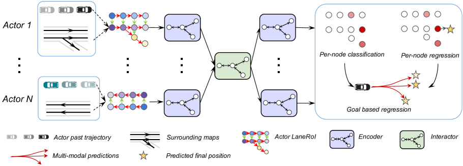
Figure 2: Overview of LaneRCNN. It first encodes each actor with our proposed LaneRoI representation, processes each LaneRoI with an encoder, and then models interactions among actors with a graph-based interactor. Finally, LaneRCNN predicts final positions of actors in a fully-convolutional manner, and then decodes full trajectories based on these positions.

Although such a paradigm has shown competitive results, it has three main shortcomings: 1) Representing the context information of large regions of space, such as fast moving actors traversing possibly a hundred meters within five seconds, with a single vector is difficult. 2) Building a fully-connected interaction graph among actors ignores important map structures. For example, an unprotected left turn vehicle should yield to oncoming traffic, while two spatially nearby vehicles driving on opposite lanes barely interact with each other. 3) The regression header does not explicitly leverage the lane information, which could provide a good inductive bias for accurate predictions. As a consequence, regression-based predictors sometimes forecast shooting-out-of-road trajectories, which are unrealistic.

In this paper, we propose a graph-centric motion forecasting model, i.e., LaneRCNN, to address the aforementioned issues. We represent an actor and its context in a distributed and map-aware manner by constructing an actor-specific graph, called Lane-graph Region-of-Interest (LaneRoI), along with node embeddings that encode the past motion and map semantics. In particular, we construct LaneRoI following the topology of lanes that are relevant to this actor, where nodes on this graph correspond to small spatial regions along these lanes, and edges represent the topological and spatial relations among regions. Compared to using a single vector to encode all the information of a large region, our LaneRoI naturally preserves the map structure and captures the more fine-grained information, as each node embedding only needs to represent the local context within a small region. To model interactions, we embed the LaneRoIs of all actors to a global lane graph and then propagate the information over this global graph. Since the LaneRoI’s of interacting actors are highly relevant, those actors will share overlapping regions on the global graph, thus having more frequent communications during the information propagation compared to irrelevant actors. Importantly, this process neither requires any heuristics nor makes any oversimplified assumptions while learning interactions conditioned on maps. We then predict future motions on each LaneRoI in a fully-convolutional manner, such that small regions along lanes (nodes in LaneRoI) can serve as anchors and provide good priors . We demonstrate the effectiveness of our method on the large-scale Argoverse motion forecasting benchmark [10]. We achieve the first rank on the challenging Argoverse competition leaderboard [1], significantly outperforming previous results.

2 Related Work

Motion Forecasting:

Traditional methods use hand-crafted features and rules based on human knowledge to model interactions and constraints in motion forecasting [12, 11, 14, 21, 33, 57, 32], which are sometimes oversimplified and not scalable. Recently, learning-based approaches employ the deep learning and significantly outperform traditional ones. Given the actors and the scene, a deep forecasting model first needs to design a format to encode the information. To do so, previous methods [41, 4, 37] often rasterize the trajectories of actors into a Birds-Eye-View (BEV) image, with different channels representing different observation timesteps, and then apply a CNN and RoI pooling [39, 20] to extract actor features. Maps can be encoded similarly [59, 60, 8, 4, 49]. However, the square receptive fields of a CNN may not be efficient to encode actor movements [29], which are typically long curves. Moreover, the map rasterization may lose useful information like lane topologies. RNNs are an alternative way to encode actor kinematic information [62, 49, 16, 61, 18, 2] compactly and efficiently. Recently, VectorNet [16] and LaneGCN [29] generalized such compact encodings to map representations. VectorNet treats a map as a collection of polylines and uses a RNN to encode them, while LaneGCN builds a graph of lanes and conducts convolutions over the graph. Different from all these work, we encode both actors and maps in an unified graph representation, which is more structured and powerful.

Modeling interactions among actors is also critical for a multi-agent system. Pioneering learning-based work design a social-pooling mechanism [2, 18] to aggregate the information from nearby actors. However, such a pooling operation may potentially lose actor-specific information. To address this, attention-mechanism [43, 52, 44, 48] or GNN-based methods [60, 26, 29, 6, 41, 49, 7, 16] build actor interaction graphs (usually fully-connected with all actors or k-nearest neighbors based), and perform attention or message passing to update actor features. Social convolutional pooling [62, 15, 47] has also been explored, which maintains the spatial distribution of actors. However, most of these work do not explicitly consider map structures, which largely affects interactions among actors in reality.

To generate each actor’s predicted futures, many works sample multi-modal futures under a conditional variational auto-encoder (CVAE) framework [25, 40, 49, 41, 7], or with a multi-head/mode regressor [29, 13, 34]. Others output discrete sets of trajectory samples [60, 37, 9] or occupancy maps [22, 42]. Recently, TNT [61] concurrently and independently designs a similar output parameterization as ours where lanes are used as priors for the forecasting. Note that, in addition to the parameterization, we contribute a novel graph representation and a powerful architecture which significantly outperforms their results.

Graph Neural Networks:

Relying on operators like graph convolution and message passing, graph neural networks (GNNs) and their variants [45, 5, 28, 24, 19, 31] generalize deep learning on regular graphs like grids to ones with irregular topologies. They have achieved great successes in learning useful graph representations for various tasks [35, 38, 50, 27, 17]. We draw inspiration from the general concept “ego-graph” and propose LaneRoI, which is specially designed for lane graphs and captures both the local map topologies and the past motion information of an individual actor. Moreover, to capture interactions among actors, we further propose an interaction module which effectively communicates information among LaneRoI graphs.

3 LaneRCNN

Our goal is to predict the future motions of all actors in a scene, given their past motions and an HD map. Different from existing work, we represent an actor and its context with a LaneRoI, an actor-specific graph which is more structured and expressive than the single feature vector used in the literature. Based on this representation, we design LaneRCNN, a graph-centric motion forecasting model that encodes context, models interactions between actors, and predicts future motions all in a map topology aware manner. An overview of our model is shown in Fig. 2.

In the following, we first introduce our problem formulation and notations in Sec. 3.1. We then define our LaneRoI representations in Sec. 3.2. In Sec. 3.3, we explain how LaneRCNN processes features and models interactions via graph-based message-passing. Finally, we show our map-aware trajectory prediction and learning objectives in Sec. 3.4 and Sec. 3.5 respectively.

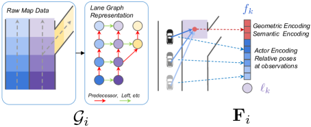
Figure 3: The LaneRoI of the actor $i$ is a collection of a graph $\mathcal{G}_{i}$ (constructed following lane topology: nodes as lane segments and edges as segment connectivities) and node embeddings $\mathbf{F}_{i}$ (encoding motions of the actor, as well as geometric and semantic properties of lane segments).

3.1 Problem Formulation

We denote the past motion of the $i$-th actor as a set of 2D points encoding the center locations over the past $L$ timesteps, i.e., $\left\{(x_{i}^{-L},y_{i}^{-L}),\cdots,(x_{i}^{-1},y_{i}^{-1})\right\}$, with $(x,y)$ the 2D coordinates in bird’s eye view (BEV). Our goal is to forecast the future motions of all actors in the scene $\left\{(x_{i}^{0},y_{i}^{0}),\cdots,(x_{i}^{T},y_{i}^{T})|i=1,\cdots,N\right\}$, where $T$ is our prediction horizon and $N$ is the number of actors.

In addition to the past kinematic information of the actors, maps also play an important role for motion forecasting since (i) actors usually follow lanes on the map, (ii) the map structure determines the right of way, which in turns affects the interactions among actors. As is common practice in self-driving, we assume an HD map is accessible, which contains lanes and associated semantic attributes, e.g., turning lane and lane controlled by traffic light. Each lane is composed of many consecutive lane segments $\ell_{i}$, which are short segments along the centerline of the lane. In addition, a lane segment $\ell_{i}$ can have pairwise relationships with another segment $\ell_{j}$ in the same lane or in another lane, such as $\ell_{i}$ being a successor of $\ell_{j}$ or a left neighbor.

3.2 LaneRoI Representation

Graph Representation:

One straight-forward way to represent an actor and its context (map) information is by first rasterizing both its trajectory as well as the map to form a 2D BEV image, and then cropping the underlying representation centered in the actor’s location in BEV [60, 49, 62, 6]. However, rasterizations are prone to information loss such as connectivities among lanes. Furthermore, it is a rather inefficient representation since actor motions are expanded typically in the direction along the lanes, not across them. Inspired by [29], we instead use a graph representation for our LaneRoI to preserve the structure while being compact. For each actor $i$ in the scene, we first retrieve all relevant lanes that this actor can possibly go to in the prediction horizon $T$ as well as come from in the observed history horizon $L$. We then convert the lanes into a directed graph $\mathcal{G}_{i}=\{\mathcal{V},\{\mathcal{E}_{\text{suc}},\mathcal{E}_{\text{pre}},\mathcal{E}_{\text{left}},\mathcal{E}_{\text{right}}\}\}$ where each node $v\in\mathcal{V}$ represents a lane segment within those lanes and the lane topology is represented by different types of edges $\mathcal{E}_{r}$, encoding the following relationships: predecessor, successor, left and right neighbor. Two nodes are connected by an edge $e\in\mathcal{E}_{r}$ if the corresponding lane segments $\ell_{i},\ell_{j}$ have a relation $r$, e.g., lane segment $\ell_{i}$ is a successor of lane segment $\ell_{j}$. Hereafter, we will use the term node interchangeably with the term lane segment.

Graph Input Encoding:

The graph $\mathcal{G}_{i}$ only characterizes map structures around the $i$-th actor without much information about the actor. We therefore augment the graph with a set of node embeddings to construct our LaneRoI . Recall that each node $k$ in $\mathcal{G}_{i}$ is associated with a lane segment $\ell_{k}$. We design its embedding $f_{k}\in\mathbb{R}^{C}$ to capture the geometric and semantic information of $\ell_{k}$, as well as its relations with the actor. In particular, geometric features include the center location, the orientation and the curvature of $\ell_{k}$; semantic features include binary features indicating if $\ell_{k}$ is a turning lane, if it is currently controlled by a red light, etc. To encode the actor information into $f_{k}$, we note that the past motion of an actor can be identified as a set of 2D displacements, defining the movements between consecutive timesteps. Therefore, we also include the relative positions and orientations of these 2D displacements w.r.t. $\ell_{k}$ into $f_{k}$ which encodes actor motions in a map-dependent manner. This is beneficial for understanding actor behaviors w.r.t. the map, e.g., a trajectory that steadily deviates from one lane and approaches the neighboring lane is highly likely a lane change. In practice, it is important to clamp the actor information, i.e., if $\ell_{k}$ is more than 5 meters away from the actor we replace the actor motion embedding in $f_{k}$ with zeros. We hypothesize that such a restriction encourages the model to learn better representations via the message passing over the graph. To summarize, $(\mathcal{G}_{i},\mathbf{F}_{i})$ is the LaneRoI of the actor $i$, encoding the actor-specific information for motion forecasting, where $\mathbf{F}_{i}\in\mathbb{R}^{M_{i}\times C}$ is the collection of node embeddings $f_{k}$ and $M_{i}$ is the number of nodes in $\mathcal{G}_{i}$.

3.3 LaneRCNN Backbone

As LaneRoIs have irregular graph structures, we can not apply standard 2D convolutions to obtain feature representations. In the following, we first introduce the lane convolution and pooling operators (Fig. 4), which serve similar purposes as their 2D counterparts while respecting the graph topology. Based on these operators, we then describe how our LaneRCNN updates features of each LaneRoI as well as handles interactions among all LaneRoIs (actors).

Lane Convolution Operator:

We briefly introduce the lane convolution which was originally proposed in [29] Given a LaneRoI $(\mathcal{G}_{i},\mathbf{F}_{i})$, a lane convolution updates features $\mathbf{F}_{i}$ by aggregating features from its neighborhood (in the graph). Formally, we use $\mathcal{E}_{i}(r)$ to denote the binary adjacency matrix for $\mathcal{G}_{i}$ under the relation $r$, i.e., the $(p,q)$ entry in this matrix is $1$ if lane segments $\ell_{p}$ and $\ell_{q}$ have the relation $r$ and $0$ otherwise. We denote the $n$-hop connectivity under the relation $r$ as the matrix $\operatorname{bool}\left(\mathcal{E}_{i}(r)\cdot\mathcal{E}_{i}(r)\cdots\mathcal{E}_{i}(r)\right)=\operatorname{bool}\left(\mathcal{E}_{i}^{n}(r)\right)$, where the operator $\operatorname{bool}$ sets any non-zero entries to one and otherwise keeps them as zero. The output node features are updated as follows,

$$\mathbf{F}_{i}\leftarrow\Psi\left(\mathbf{F}_{i}\mathbf{W}+\sum_{r,n}\operatorname{bool}\left(\mathcal{E}_{i}^{n}(r)\right)\mathbf{F}_{i}\mathbf{W}_{n,r}\right),$$ (1)

where both $\mathbf{W}$ and $\mathbf{W}_{n,r}$ are learnable parameters, $\Psi(\cdot)$ is a non-linearity consisted of LayerNorm [3] and ReLU [36], and the summation is over all possible relations $r$ and hops $n$. In practice, we use $n\in\left\{1,2,4,8,16,32\right\}$. Such a multi-hop mechanism mimics the dilated convolution [58] and effectively enlarges the receptive field.

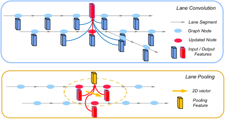
Figure 4: An illustration for lane convolution and lane pooling operators, which have similar functionalities as their 2D counterparts while respecting the lane topology.

Lane Pooling Operator:

We design a lane pooling operator which is a learnable pooling function. Given a LaneRoI $(\mathcal{G}_{i},\mathbf{F}_{i})$, recall $\mathcal{G}_{i}$ actually corresponds to a number of lanes spanned in the 2D plane (scene). For an arbitrary 2D vector $\mathbf{v}$ in the plane, a lane pooling operator pools, or ‘interpolates’, the feature of $\mathbf{v}$ from $\mathbf{F}_{i}$. Note that $\mathbf{v}$ can be a lane segment in another graph $\mathcal{G}_{j}$ (spatially close to $\mathcal{G}_{i}$). Therefore, lane pooling helps communicate information back and forth between graphs, which we will explain in the interaction part. To generate the feature $f_{\mathbf{v}}$ of vector $\mathbf{v}$, we first retrieve its ‘neighboring nodes’ in $\mathcal{G}_{i}$, by checking if the center distance between a lane segment $\ell_{k}$ in $\mathcal{G}_{i}$ and vector $\mathbf{v}$ is smaller than a certain threshold. A naive pooling strategy is to simply take a mean of those $\ell_{k}$. However, this ignores the fact that relations between $\ell_{k}$ and $\mathbf{v}$ can vary a lot depending on their relative pose: a lane segment that is perpendicular to $\mathbf{v}$ (conflicting) and the one that is aligned with $\mathbf{v}$ have very different semantics. Inspired by the generalized convolution on graphs/manifolds [35, 53, 29], we use the relative pose and some non-linearities to learn a pooling function. In particular, we denote the set of surrounding nodes on $\mathcal{G}_{i}$ as $\mathcal{N}$, and the relative pose between $\mathbf{v}$ and $\ell_{k}$ as $\Delta_{\mathbf{v}k}$ which includes relative position and orientation. The pooled feature $f_{\mathbf{v}}$ can then be written as,

$$f_{\mathbf{v}}=\mathcal{M}_{b}\left(\sum_{k\in\mathcal{N}}\mathcal{M}_{a}\left(\left[f_{k},\Delta_{\mathbf{v}k}\right]\right)\right),$$ (2)

where $[\cdots]$ means concatenation and $\mathcal{M}$ is a two-layer multi-layer perceptron (MLP).

LaneRoI Encoder:

Equipped with operators introduced above, we now describe how LaneRCNN processes features for each LaneRoI. Given a scene, we first construct a LaneRoI per actor and encode its input information into node embeddings as described in Sec. 3.2. Then, for each LaneRoI, we apply four lane convolution layers and get the updated node embeddings $\mathbf{F}_{i}$. Essentially, a lane convolution layer propagates information from a node to its (multi-hop) connected nodes. Stacking more layers builds larger receptive fields and has a larger model capacity. However, we find deeper networks do not necessarily lead to better performances in practice, possibly due to the well-known difficulty of learning long-term dependencies. To address this, we introduce a graph shortcut mechanism on LaneRoI. The graph shortcut layer can be applied after any layer of lane convolution: we aggregate $\mathbf{F}_{i}$ output from the previous layer into a global embedding with the same dimension as node embeddings, and then add it to embeddings of all nodes in $\mathcal{G}_{i}$. Recall that the actor past motions are a number of 2D vectors, i.e., movements between consecutive timesteps. We use the lane pooling to extract features for these 2D vectors. A 1D CNN with downsampling is then applied to these features to build the final shortcut embedding. Intuitively, a lane convolution may suffer from the diminishing information flow during the message-passing, while such a shortcut can provide an auxiliary path to communicate among far-away nodes efficiently. We will show that the shortcut significantly boosts the performance in the ablation study.

LaneRoI Interactor:

So far, our LaneRoI encoder provides good features for a given actor, but it lacks the ability to model interactions among different actors, which is extremely important for the motion forecasting in a multi-agent system. We now describe how we handle actor interactions under LaneRoI representations. After processing all LaneRoIs with the LaneRoI encoder (shared weights), we build a global lane graph $\mathcal{G}$ containing all lanes in the scene. Its node embeddings are constructed by projecting all LaneRoIs to $\mathcal{G}$ itself. We then apply four lane convolution layers on $\mathcal{G}$ to perform message passing. Finally, we distribute the ‘global node’ embeddings back to each LaneRoI . Our design is motivated by the fact that actors have interactions since they share the same space-time region. Similarly, in our model, all LaneRoIs share the same global graph $\mathcal{G}$ where they communicate with each other following map structures.

In particular, suppose we have a set of LaneRoIs $\{(\mathcal{G}_{i},\mathbf{F}_{i})|i=1,\cdots,N\}$ encoded from previous layers and a global lane graph $\mathcal{G}$. For each node in $\mathcal{G}$, we use a lane pooling to construct its embedding: retrieving its neighbors from all LaneRoIs as $\mathcal{N}$, measured by center distance, and then applying Eq. 2. This ensures each global node has the information of all those actors that could interact with it. The distribute step is an inverse process: for each node in $\mathcal{G}_{i}$, find its neighbors, apply a lane pooling, and add the resulted embedding to original $\mathbf{F}_{i}$ (serving as a skip-connection).

	Method	K=1			K=6
		minADE	minFDE	MR	minADE	minFDE	MR
Argoverse Baseline [10]	NN	3.45	7.88	87.0	1.71	3.28	53.7
	NN+map	3.65	8.12	94.0	2.08	4.02	58.0
	LSTM+map	2.92	6.45	75.0	2.08	4.19	67.0
Leaderboard [1]	TNT (4th) [61]	1.78	3.91	59.7	0.94	1.54	13.3
	Jean (3rd) [34]	1.74	4.24	68.6	1.00	1.42	13.1
	Poly (2nd) [1]	1.71	3.85	59.6	0.89	1.50	13.1
	Ours-LaneRCNN (1st)	1.69	3.69	56.9	0.90	1.45	12.3

Table 1: Argoverse Motion Forecasting Leaderboard. All metrics are lower the better and Miss-Rate (MR, K=6) is the official ranking metric.

3.4 Map-Relative Outputs Decoding

The future is innately multi-modal and an actor can take many different yet possible future motions. Fortunately, different modalities can be largely characterized by different goals of an actor. Here, a goal means a final position of an actor at the end of prediction horizon. Note that actors mostly follow lane structures and thus their goals are usually close to a lane segment $\ell$. Therefore, our model can predict the final goals of an actor in a fully convolutional manner, based on its LaneRoI features. Namely, we apply a 2-layer MLP on each node feature $f_{k}$, and output five values including the probability that $\ell_{k}$ is the closest lane segment to final destination $p(\ell_{k}=\text{goal})$, as well as relative residues from $\ell_{k}$ to the final destination $x_{gt}-x_{k}$, $y_{gt}-y_{k}$, $\sin(\theta_{gt}-\theta_{k})$, $\cos(\theta_{gt}-\theta_{k})$.

Based on results of previous steps, we select the top K For each prediction, we use the position and the direction of the actor at $t=0$ as well as those at the goal to interpolate a curve, using Bezier quadratic parameterization. We then unroll a constant acceleration kinematic model along this curve, and sample 2D points at each future timestep based on the curve and the kinematic information. These 2D points form a trajectory, which serves as an initial proposal of our final forecasting. Despite its simplicity, this parameterization gives us surprisingly good results.

Our final step is to refine those trajectory proposals using a learnable header. Similar to the shortcut layer introduced in Sec. 3.3, we use a lane pooling followed by a 1D CNN to pool features of this trajectory. Finally, we decode a pair of values per timestep, representing the residue from the trajectory proposal to the ground-truth future position at this timestep (encoded in Frenet coordinate of this trajectory proposal). We provide more detailed definitions of our parameterization and output space in the supplementary A.

3.5 Learning

We train our model end-to-end with a loss containing the goal classification, the goal regression, and the trajectory refinements. Specifically, we use

$$\mathcal{L}=\mathcal{L}_{\text{cls}}+\alpha\mathcal{L}_{\text{reg}}+\beta\mathcal{L}_{\text{refine}},$$

where $\alpha$ and $\beta$ are hyparameters determining relative weights of different terms. As our model predicts the goal classification and regression results per node, we simply adopt a binary cross entropy loss for $\mathcal{L}_{\text{cls}}$ with online hard example mining [46] and a smooth-L1 loss for $\mathcal{L}_{\text{reg}}$, where the $\mathcal{L}_{\text{reg}}$ is only evaluated on positive nodes, i.e. closest lane segments to the ground-truth final positions. The $\mathcal{L}_{\text{refine}}$ is also a smooth-L1 loss with training labels generated on the fly: projecting ground-truth future trajectories to the predicted trajectory proposals, and use the Frenet coordinate values as our regression targets.

Module	Ablation		K=1		K=6
			minADE	minFDE	minADE	minFDE	MR
LaneRoI Encoder	LaneRoI	Shortcut
			1.68	3.79	0.86	1.46	14.5
	✓		1.68	3.84	0.82	1.36	12.9
	✓	Global Pool	1.69	3.84	0.84	1.38	12.8
	✓	Center Pool	1.67	3.80	0.83	1.35	12.4
	✓	Ours x 1	1.55	3.45	0.81	1.29	11.1
	✓	Ours x 2	1.54	3.45	0.80	1.29	10.8
LaneRoI Interactor	Interactor-Arch	Pooling
			1.54	3.45	0.80	1.29	10.8
	Attention	Global	1.42	3.10	0.78	1.24	9.8
	Attention	Shortcut	1.47	3.22	0.80	1.25	10.1
	GNN	Global	1.45	3.15	0.79	1.25	9.9
	GNN	Shortcut	1.45	3.21	0.79	1.25	10.0
	Ours	AvgPool	1.42	3.11	0.79	1.25	9.9
	Ours	LanePool	1.33	2.85	0.77	1.19	8.2

Table 2: Ablations on different modules of LaneRCNN. Metrics are reported on the validation set. In the upper half, we examine our LaneRoI Encoder, comparing per-actor 1D feature vector v.s. LaneRoI representations as well as different designs for the shortcut mechanism. In the lower half, we compare different strategies to model interactions, including a fully connected graph among actors with GNN / attention, as well as ours. Pooling refers to how we pool a 1D actor feature from each LaneRoI which are used by GNN / attention. Rows shaded in gray indicate the architecture used in our final model.

4 Experiment

We evaluate the effectiveness of LaneRCNN on the large-scale Argoverse motion forecasting benchmark (Argoverse), which is publicly available and provides annotations of both actor motions and HD maps. In the following, we first explain our experimental setup and then compare our method against state-of-the-art on the leaderboard. We also conduct ablation studies on each module of LaneRCNN to validate our design choices. Finally, we present some qualitative results.

4.1 Experimental Settings

Dataset:

Argoverse provides a large-scale dataset [10] for the purpose of training, validating and testing models, where the task is to forecast 3 seconds future motions given 2 seconds past observations. This dataset consists of more than 30K real-world driving sequences collected in Miami and Pittsburgh. Those sequences are further split into train, validation, and test sets without any geographical overlapping. Each of them has 205942, 39472, and 78143 sequences respectively. In particular, each sequence contains the positions of all actors in a scene within the past 2 seconds history, annotated at 10Hz. It also specifies one interesting actor in this scene, with type ‘agent’, whose future 3 seconds motions are used for the evaluation. The train and validation splits additionally provide future locations of all actors within 3 second horizon labeled at 10Hz, while annotations for test sequences are withheld from the public and used for the leaderboard evaluation. Besides, HD map information can be retrieved for all sequences.

Metrics:

We follow the benchmark setting and use Miss-Rate (MR), Average Displacement Error (ADE) and Final Displacement Error (FDE), which are also widely used in the community. MR is defined as the ratio of data that none of the predictions has less than 2.0 meters L2 error at the final timestep. ADE is the averaged L2 errors of all future timesteps, while FDE only counts the final timestep. To evaluate the mutli-modal prediction, we also adopt the benchmark setting: predicting K=6 future trajectories per actor and evaluating the $\text{min}_{K}\text{MR}$, $\text{min}_{K}\text{ADE}$, $\text{min}_{K}\text{FDE}$ using the trajectory that is closest to the ground-truth.

Implementation Details:

We train our model on the train set with the batch size of 64 and terminate at 30 epochs. We use Adam [23] optimizer with the learning rate initialized at 0.01 and decayed by 10 at 20 epochs. To normalize the data, we translate and rotate the coordinate system of each sequence so that the origin is at current position ($t=0$) of ‘agent’ actor and x-axis is aligned with its current direction. During training, we further apply a random rotation data augmentation within $(-\frac{2}{3}\pi,\frac{2}{3}\pi)$. No other data processing is applied such as label smoothing. More implementation details are provided in the supplementary C.

4.2 Comparison with State-of-the-art

We compare our approach with top entries on Argoverse motion forecasting leaderboard [1] as well as official baselines provided by the dataset [10] as shown in Table 1. We only submit our final model once to the leaderboard and achieve state-of-the-art performance. This is a very challenging benchmark with around 100 participants at the time of our submission. Note that for the official ranking metric MR (K=6), previous leading methods are extremely close to each other, implying the difficulty of further improving the performance. Nevertheless, we significantly boost the number which verifies the effectiveness of our method. Among the competitors, both Jean [34] and TNT [61] use RNNs to encode actor kinematic states and lane polylines. They then build a fully-connected interaction graph among all actors and lanes, and use either the attention or GNNs to model interactions. As a result, they represent each actor with a single feature vector, which is less expressive than our LaneRoI representations. Moreover, the fully-connected interaction graph may also discard valuable map structure information. Note that TNT shares a similar output parameterization as ours, yet we perform better on all metrics. This further validates the advantages of our LaneRoI compared against traditional representations. Unfortunately, since Poly team does not publish their method, we can not compare with it qualitatively.

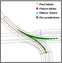
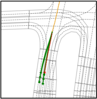
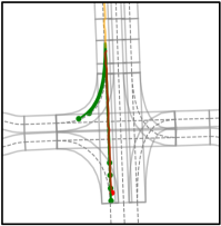
Figure 5: Qualitative results on Argoverse validation set. Here we show (from left-to-right): 1) curved lanes 2) lane changing 3) intersection 4) overtaking.

4.3 Ablation Studies

Ablations on LaneRoI Encoder:

We first show the ablation study on one of our main contributions, i.e., LaneRoI , in the upper half of Table 2. The first row shows a representative of the traditional representations. Specifically, we first build embeddings for lane graph nodes using only the map information and 4 lane convolution layers. We then use a 1D CNN (U-net style) to extract a motion feature vector from actor kinematic states, concatenate it with every graph node embedding and make predictions. Conceptually, this is similar to TNT [61] except that we modify the backbone network to make comparisons fair. On the second row, we show the result of our LaneRoI representations with again four lane convolution layers (no shortcuts). Hence, the only difference is whether the actor is encoded with a single motion vector shared by all nodes, or encoded in a distributed and structured manner as ours. As shown in the table, our LaneRoI achieves similar or better results on all metrics, exhibiting its advantages. Note that this row is not yet our best result in terms of using LaneRoI representations, as the actor information is only exposed to a small region during the input encoding (clamping at input node embeddings) and can not efficiently propagate to the full LaneRoI without the help of the shortcut, which we will show next.

Subsequent rows in Table 2 compare different design choices for the shortcut mechanism, in particular how we pool the global feature for each LaneRoI. ‘Global Pool’ refers to average-pooling all node embeddings within a LaneRoI, and ‘Center Pool’ means we pool a feature from a LaneRoI using nodes that around the last observation of the actor and a lane pooling. As we can see, although these two approaches can possibly spread out information to every node in a LaneRoI (and thus build a shortcut), they barely improve the performance. On the contrary, ours achieve significant improvements. This is because we pool features along the past trajectory of the actor, which results in a larger and actor-motion-specific receptive field. Here, $\times 1$ and $\times 2$ refer to an encoder with 1 shortcut per 4 and 2 lane convolution layers respectively. This shows stacking more shortcuts provides some, but diminishing, benefits.

Ablations on LaneRoI Interactor:

To verify the effectiveness of our map-aware interaction module, we compare against several model variants based on the fully-connected interaction graph among actors. Specifically, for each actor, we apply a LaneRoI encoder to process node embeddings, and then pool an actor-specific feature vector from LaneRoI via either the global average pooling or our shortcut mechanism. These actor features are then fed into a transformer-style [51] attention module or a fully-connected GNN. Finally, we add the output actor features to nodes in their LaneRoI respectively and make predictions using our decoding module. As a result, these variants have the same pipeline as ours, with the only difference on how to communicate across actors. To make comparisons as fair as possible, both the attention and GNN have the same numbers of layers and channels as our LaneRoI Interactor.

As shown in Table 2, all interaction-based models outperform the one without considering interactions (row 1) as expected. In addition, our approach significantly improves the performance compared to both the attention and GNN. Interestingly, all fully-connected interaction graph based model reach similar performance, which might imply such backbones may saturate the performance (as also shown by leading methods on the leaderboard). We also show that naively using the average pooling to embed features from LaneRoIs to global graph does not achieves good performance because it ignores local structures.

4.4 Qualitative results

In Figure 5, we show some qualitative results on Argoverse validation set. We can see that our method generally follows the map very well and demonstrates good multi-modalities. From left to right, we show 1) when an actor follows a curved lane, our model predicts two direction modes with different velocities; 2) when it is on a straight lane, our model covers the possibilities of lane changing; 3) when it’s approaching an intersection, our model captures both the go-straight and the turn-right modes, especially with lower speeds for turning right, which are quite common in the real world; 4) when there is an actor blocking the path, we predict overtaking behaviors matching exactly with the ground-truth. Moreover, for the lane-following mode, we predict much slower speeds which are consistent with this scenario, showing the effectiveness of our interaction modeling. We provide more qualitative results in the supplementary E.

5 Conclusion

In this paper, we propose LaneRCNN, a graph-centric motion forecasting model. Relying on learnable graph operators, LaneRCNN builds a distributed lane-graph-based representation (LaneROI) per actor to encode its past motion and the local map topology. Moreover, we propose an interaction module which effectively captures the interactions among actors within the shared global lane graph. And lastly, we parameterize the output trajectory using lane graphs which helps improve the prediction. We demonstrate that LaneRCNN achieves state-of-the-art performance on the challenging Argoverse motion forecasting benchmark.

Appendix A Map-Relative Output Decoding

Our output decoding can be divided into three steps: predicting the final goal of an actor based on node embeddings, propose an initial trajectory based on the goal and the initial pose, and refine the trajectory proposal with a learnable header. As the first step is straight-forward, we now explain how we perform the second and third steps in details.

A.1 Trajectory Proposal

Given a predicted final pose $\left(x^{T},y^{T},dx^{T},dy^{T}\right)$ and initial pose $\left(x^{0},y^{0},dx^{0},dy^{0}\right)$ of an actor, where $(x,y)$ is the 2D location and $(dx,dy)$ is the tangent vector, we fit a Bezier quadratic curve satisfying these boundary conditions, i.e., zero-th and first order derivative values. Specifically, the curve can be parameterized by

$$x(s) =a_{0}s^{2}+a_{1}s+a_{2},$$

$$y(s) =b_{0}s^{2}+b_{1}s+b_{2},$$

$$s.t.\quad x(0) =x^{0},\quad x(1)=x^{T},\quad\frac{x^{\prime}(0)}{x^{\prime}(1)}=\frac{dx^{0}}{dx^{T}},$$

$$y(0) =y^{0},\quad y(1)=y^{T},\quad\frac{y^{\prime}(0)}{y^{\prime}(1)}=\frac{dy^{0}}{dy^{T}}.$$

Here, $s$ is the normalized distance. As a result, each predicted goal uniquely defines a 2D curve.

Next, we unroll a velocity profile along this curve to get 2D waypoint proposals at every future timestamp. Assuming the actor is moving with a constant acceleration within the prediction horizon, we can compute the acceleration based on the initial velocity $v$ and the traveled distance $s$ (from $(x^{0},y^{0})$ to $(x^{T},y^{T})$ along the Bezier curve) using

$$a=\frac{2\times(s-vT)}{T^{2}}.$$

Therefore, the future position of the actor at any timestamp $t$ can be evaluated by querying the position along the curve at $s(t)=vt+\frac{1}{2}at^{2}$.

A.2 Trajectory Refinement

Simply using our trajectory proposals for motion forecasting will not be very accurate, as not all actors move with constant accelerations and follow Bezier curves, yet the proposals provide us good initial estimations which we can further refine. To do so, for each trajectory proposal, we construct its features using a shortcut layer on top our LaneRoI node embeddings. We then use a 2 layer MLP to decode a pair of values $\left(s^{t},d^{t}\right)$ for each future timestamp, representing the actor position at time $t$ in the Frenet Coordinate System [56]. The Cartesian coordinates $\left(x^{t},y^{t}\right)$ can be mapped from $\left(s^{t},d^{t}\right)$ by first traversing along the Bezier curve distance $s^{t}$ (a.k.a. longitudinal), and then deviating perpendicularly from the curve distance $d^{t}$ (a.k.a. lateral). The sign of $d^{t}$ indicates the deviation is either to-the-left or to-the-right.

Sampling	Avg Length ($\ell_{k}$)	Reg	$\text{min}_{1}$ADE	$\text{min}_{1}$FDE	$\text{min}_{6}$ADE	$\text{min}_{6}$FDE	$\text{min}_{6}$MR
up 1x	2.1 m		1.52	3.32	0.94	1.69	24.0
up 1x	2.1 m	✓	1.41	3.03	0.83	1.35	14.1
up 2x	1.1 m		1.43	3.09	0.85	1.39	13.4
up 2x	1.1 m	✓	1.39	2.99	0.80	1.24	10.2
uniform	2 m		1.39	2.94	0.86	1.44	10.5
uniform	2 m	✓	1.35	2.86	0.80	1.29	8.2
uniform	1 m		1.37	2.90	0.83	1.32	9.9
uniform	1 m	✓	1.33	2.85	0.77	1.19	8.2

Table 3: Ablation studies on lane segments sampling strategy and regression branch. We compare different sampling strategies including using the original segment labels (upsample 1x) or upsample the labels (upsample 2x), as well as uniformly sample segments along lanes (uniform 2/1m). For each, we also compare using the regression branch or not (only classification branch). Our final model is shaded in grey.

Appendix B LaneRoI Construction

To construct a LaneRoI, we need to retrieve all relevant lanes of a given actor. In our experiments, we use a simple heuristic for this purpose. Given an HD map of a scene and an arbitrary actor in this scene, we first uniformly sample segments $\ell_{k}$ with 1 meter length along each lane’s centerline . Then, for the actor’s location at each past timestamp, we find the nearest lane segment and collect them together into a set. This is a simplified version of lane association and achieve very high recall of the true ego-lane. Finally, we retrieve predecessing and successing lane segments (within a range $D$) of those segments in the set to capture lane-following behaviors, as well as left and right neighbors of those predecessing and successing lanes which are necessary to capture lane-changing behaviors. The range $D$ equals to an expected length of future movement by integrating the current velocity within the prediction horizon, plus a buffer value, e.g., 20 meters. Therefore, $D$ is dynamically changed based on actor velocity. This is motivated by the fact that high speed actors travel larger distances and thus should have larger LaneRoIs to capture their motions as well as interactions with other actors.

Appendix C Architecture and Learning Details

Our LaneRCNN is constructed as follows: we first feed each input LaneRoI representation into an encoder, consists of 2 lane convolution layers and a shortcut layer, followed by another 2 lane convolution layers and a shortcut layer. We then use a lane pooling layer to build the node embeddings of the global graph (interactor), where the neighborhood threshold is set to 2 meters. Another four layers of lane convolution are applied on top of this global graph. Next, we distribute the global node embeddings to each LaneRoI by using a lane pooling layer and adding the pooled features to original LaneRoI embeddings (previous encoder outputs) as a skip-connection architecture. Another 4 layers of lane convolution and 2 layers of shortcut layers are applied afterwards. Finally, we use two layers of MLP to decode a classification score per node using its embeddings, and another two layer for regression branch as well. All layers except the final outputs have 64 channels. We use Layer Normalization [3] and ReLU [36] for normalization and non-linearity respectively.

During training, we apply online hard example mining [46] for $\mathcal{L}_{cls}$ (Eq. 3.5). Recall each node predict a binary classification score indicating whether this node is the closest lane segment to the final actor position. We use the closest lane segment to the ground-truth location as our positive example. Negative examples are all nodes deviating from the ground-truth by more than 6 meters and the remaining nodes are ‘don’t care’ which do not contribute any loss for $\mathcal{L}_{cls}$. Then, we randomly subsample one fourth of all negative examples and among them we use the hardest 100 negative examples for each data sample to compute our loss. The final $\mathcal{L}_{cls}$ is the average of positive example loss plus the average of negative example loss. Finally, we add $\mathcal{L}_{reg}$ and $\mathcal{L}_{refine}$ with relative weights of $\alpha=0.5$ and $\beta=0.2$ respectively to form our total loss $\mathcal{L}$.

Appendix D Ablation Studies

When constructing our LaneRoI, we define a lane segment $\ell$ to be a node in the graph. However, there are different ways to sample lane segments and we find such a choice largely affects the final performance. In Table 3 we show different strategies of sampling lane segments. The first four rows refer to upsampling the original lane segment labels provided in the dataset. Such a strategy provides segments with different lengths, e.g., shorter and denser segments where the geometry of the lanes changes more rapidly. The last four rows sample segments uniformly along lanes with a predefined length.

As we can observe from Table 3, even though the ‘upsample’ strategy can result in similar average segment length as the ‘uniform’ strategy, it performs much worse in all metrics. This is possible because different lengths of segments introduce additional variance and harm the representation learning process. We can also conclude from the table that using denser sampling can achieve better results. Besides, we show the effectiveness of adding a regression branch for each node in addition to a classification branch, shown in ‘Reg’ column.

Our output parameterization explicitly leverages the lane information and thus ease the training. In Fig. 6, we validate such an argument where we compare against a regression-based variant of our model. In particular, we use the same backbone as ours, and then perform a shortcut layer on top of each LaneRoI to extract an actor-specific feature vector. We then build a multi-modal regression header which directly regresses future motions in the 2D Cartesian coordinates. We can see from Fig. 6 that our model achieves decent performance when only small amounts of training data are available: with only 1% of training data, our method can achieve 20% of miss-rate. On the contrary, the regression-based model requires much more data. This shows our method can exploit map structures as good priors and ease learning.

In Table 4, we summarize ablations on different trajectory parameterizations. We can see a constant acceleration rollout slightly improves over constant speed assumption, and the Bezier curve significantly outperforms a straight line parameterization, indicating it is more realistic. In addition, adding a learnable header to refine the trajectory proposals (e.g., Bezier curve) can further boost performance.

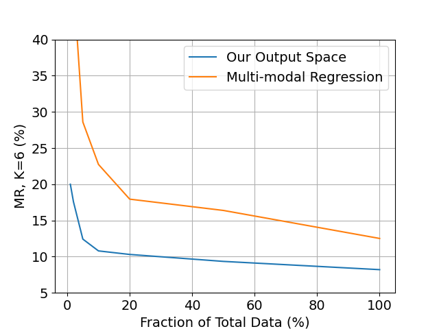
Figure 6: Model performance when using different amounts of data for training. Our output parameterization explicitly leverages lanes as priors for motion forecasting, and thus significantly ease the learning compared to directly regressing the future motions in the 2D plane.

Curve	Velocity	Learnable	$\text{min}_{1}$ADE	$\text{min}_{6}$ADE
line	const		1.53	1.04
line	acc		1.52	1.02
line	acc	✓	1.41	0.86
Bezier	const		1.46	0.96
Bezier	acc		1.44	0.94
Bezier	acc	✓	1.33	0.77

Table 4: Ablation studies on output parameterizations. We compare different ways of proposing curves (straight line v.s. Bezier quadratic curve), unrolling velocities (const as constant velocity and acc as constant acceleration), as well as using learnable refinement header or not. Our final model is shaded in grey.

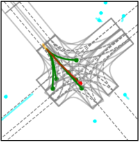
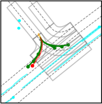
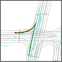
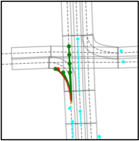
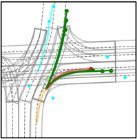
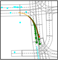
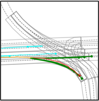
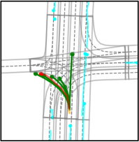
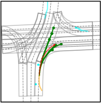
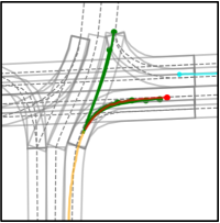
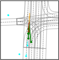
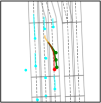
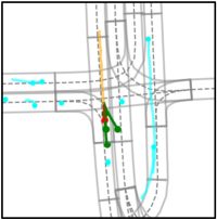
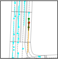
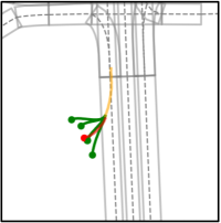
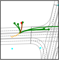
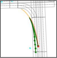
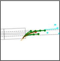
Figure 7: Qualitative results on Argoverse validation set. We show a various of scenarios including, turning (row 1-2), curved roads (row 3), breaking and overtaking (row 4), abnormal behaviors (row 5).

Appendix E Qualitative Results

Lastly, we provide more visualization of our model outputs, as we believe the metric numbers can only reveal part of the story. We present various scenarios in Fig. 7, including turning, following curved roads, interacting with other actors and some abnormal behaviors. On the first two rows, we show turning behaviors under various map topologies. We can see our motion forecasting results nicely capture possible modes: turning into different directions or occupying different lanes after turning. We also do well even if the actor is not strictly following the centerlines. On the third row, we show predictions following curved roads, which are difficult scenarios for auto-regressive predictors [59, 8]. On the fourth row, we show that our model can predict breaking or overtaking behaviors when leading vehicles are blocking the ego-actor. Finally, we show in the fifth row that our model also works well when abnormal situations occur, e.g., driving out of roads. This is impressive as the model relies on lanes to make predictions, yet it shows capabilities to predict non-map-compliant behaviors.

References

- [1] Argoverse motion forecasting competition. 2019. https://eval.ai/web/challenges/challenge-page/454/leaderboard/1279.
- [2] Alexandre Alahi, Kratarth Goel, Vignesh Ramanathan, Alexandre Robicquet, Li Fei-Fei, and Silvio Savarese. Social lstm: Human trajectory prediction in crowded spaces. In CVPR, 2016.
- [3] Jimmy Lei Ba, Jamie Ryan Kiros, and Geoffrey E Hinton. Layer normalization. arXiv, 2016.
- [4] Mayank Bansal, Alex Krizhevsky, and Abhijit Ogale. Chauffeurnet: Learning to drive by imitating the best and synthesizing the worst. arXiv, 2018.
- [5] Joan Bruna, Wojciech Zaremba, Arthur Szlam, and Yann LeCun. Spectral networks and locally connected networks on graphs. arXiv, 2013.
- [6] Sergio Casas, Cole Gulino, Renjie Liao, and Raquel Urtasun. Spatially-aware graph neural networks for relational behavior forecasting from sensor data. arXiv, 2019.
- [7] Sergio Casas, Cole Gulino, Simon Suo, Katie Luo, Renjie Liao, and Raquel Urtasun. Implicit latent variable model for scene-consistent motion forecasting. In ECCV, 2020.
- [8] Sergio Casas, Wenjie Luo, and Raquel Urtasun. Intentnet: Learning to predict intention from raw sensor data. In Proceedings of The 2nd Conference on Robot Learning, 2018.
- [9] Yuning Chai, Benjamin Sapp, Mayank Bansal, and Dragomir Anguelov. Multipath: Multiple probabilistic anchor trajectory hypotheses for behavior prediction. arXiv, 2019.
- [10] Ming-Fang Chang, John Lambert, Patsorn Sangkloy, Jagjeet Singh, Slawomir Bak, Andrew Hartnett, De Wang, Peter Carr, Simon Lucey, Deva Ramanan, et al. Argoverse: 3d tracking and forecasting with rich maps. In CVPR, 2019.
- [11] Wongun Choi and Silvio Savarese. A unified framework for multi-target tracking and collective activity recognition. In ECCV, 2012.
- [12] Wongun Choi and Silvio Savarese. Understanding collective activitiesof people from videos. PAMI, 2013.
- [13] Henggang Cui, Vladan Radosavljevic, Fang-Chieh Chou, Tsung-Han Lin, Thi Nguyen, Tzu-Kuo Huang, Jeff Schneider, and Nemanja Djuric. Multimodal trajectory predictions for autonomous driving using deep convolutional networks. In ICRA, 2019.
- [14] Nachiket Deo, Akshay Rangesh, and Mohan M Trivedi. How would surround vehicles move? a unified framework for maneuver classification and motion prediction. IEEE Transactions on Intelligent Vehicles, 2018.
- [15] Nachiket Deo and Mohan M Trivedi. Convolutional social pooling for vehicle trajectory prediction. In CVPR, 2018.
- [16] Jiyang Gao, Chen Sun, Hang Zhao, Yi Shen, Dragomir Anguelov, Congcong Li, and Cordelia Schmid. Vectornet: Encoding hd maps and agent dynamics from vectorized representation. In CVPR, 2020.
- [17] Victor Garcia and Joan Bruna. Few-shot learning with graph neural networks. In ICLR, 2018.
- [18] Agrim Gupta, Justin Johnson, Li Fei-Fei, Silvio Savarese, and Alexandre Alahi. Social gan: Socially acceptable trajectories with generative adversarial networks. In CVPR, 2018.
- [19] Will Hamilton, Zhitao Ying, and Jure Leskovec. Inductive representation learning on large graphs. In NeurIPS, 2017.
- [20] Kaiming He, Georgia Gkioxari, Piotr Dollár, and Ross Girshick. Mask r-cnn. In ICCV, 2017.
- [21] Dirk Helbing and Peter Molnar. Social force model for pedestrian dynamics. Physical review E, 1995.
- [22] Ajay Jain, Sergio Casas, Renjie Liao, Yuwen Xiong, Song Feng, Sean Segal, and Raquel Urtasun. Discrete residual flow for probabilistic pedestrian behavior prediction. arXiv, 2019.
- [23] Diederik P Kingma and Jimmy Ba. Adam: A method for stochastic optimization. arXiv, 2014.
- [24] Thomas N Kipf and Max Welling. Semi-supervised classification with graph convolutional networks. arXiv, 2016.
- [25] Namhoon Lee, Wongun Choi, Paul Vernaza, Christopher B Choy, Philip HS Torr, and Manmohan Chandraker. Desire: Distant future prediction in dynamic scenes with interacting agents. In CVPR, 2017.
- [26] Lingyun Li, Bin Yang, Ming Liang, Wenyuan Zeng, Mengye Ren, Sean Segal, and Raquel Urtasun. End-to-end contextual perception and prediction with interaction transformer. In IROS, 2020.
- [27] Ruiyu Li, Makarand Tapaswi, Renjie Liao, Jiaya Jia, Raquel Urtasun, and Sanja Fidler. Situation recognition with graph neural networks. In ICCV, 2017.
- [28] Yujia Li, Daniel Tarlow, Marc Brockschmidt, and Richard Zemel. Gated graph sequence neural networks. arXiv, 2015.
- [29] Ming Liang, Bin Yang, Rui Hu, Yun Chen, Renjie Liao, Song Feng, and Raquel Urtasun. Learning lane graph representations for motion forecasting. In ECCV, 2020.
- [30] Ming Liang, Bin Yang, Wenyuan Zeng, Yun Chen, Rui Hu, Sergio Casas, and Raquel Urtasun. Pnpnet: End-to-end perception and prediction with tracking in the loop. In CVPR, 2020.
- [31] Renjie Liao, Zhizhen Zhao, Raquel Urtasun, and Richard Zemel. Lanczosnet: Multi-scale deep graph convolutional networks. In ICLR, 2019.
- [32] Wei-Chiu D. Ma, De-An Huang, Namhoon Lee, and Kris M Kitani. Forecasting interactive dynamics of pedestrians with fictitious play. In CVPR, 2017.
- [33] Ramin Mehran, Alexis Oyama, and Mubarak Shah. Abnormal crowd behavior detection using social force model. In CVPR, 2009.
- [34] Jean Mercat, Thomas Gilles, Nicole El Zoghby, Guillaume Sandou, Dominique Beauvois, and Guillermo Pita Gil. Multi-head attention for multi-modal joint vehicle motion forecasting. In ICRA, 2020.
- [35] Federico Monti, Davide Boscaini, Jonathan Masci, Emanuele Rodola, Jan Svoboda, and Michael M Bronstein. Geometric deep learning on graphs and manifolds using mixture model cnns. In CVPR, 2017.
- [36] Vinod Nair and Geoffrey E Hinton. Rectified linear units improve restricted boltzmann machines. In ICML, 2010.
- [37] Tung Phan-Minh, Elena Corina Grigore, Freddy A Boulton, Oscar Beijbom, and Eric M Wolff. Covernet: Multimodal behavior prediction using trajectory sets. In CVPR, 2020.
- [38] Xiaojuan Qi, Renjie Liao, Jiaya Jia, Sanja Fidler, and Raquel Urtasun. 3d graph neural networks for rgbd semantic segmentation. In ICCV, 2017.
- [39] Shaoqing Ren, Kaiming He, Ross Girshick, and Jian Sun. Faster r-cnn: Towards real-time object detection with region proposal networks. In NeurIPS, 2015.
- [40] Nicholas Rhinehart, Kris M Kitani, and Paul Vernaza. R2p2: A reparameterized pushforward policy for diverse, precise generative path forecasting. In ECCV, 2018.
- [41] Nicholas Rhinehart, Rowan McAllister, Kris Kitani, and Sergey Levine. Precog: Prediction conditioned on goals in visual multi-agent settings. arXiv, 2019.
- [42] Abbas Sadat, Sergio Casas, Mengye Ren, Xinyu Wu, Pranaab Dhawan, and Raquel Urtasun. Perceive, predict, and plan: Safe motion planning through interpretable semantic representations. In ECCV, 2020.
- [43] Amir Sadeghian, Vineet Kosaraju, Ali Sadeghian, Noriaki Hirose, Hamid Rezatofighi, and Silvio Savarese. Sophie: An attentive gan for predicting paths compliant to social and physical constraints. In CVPR, 2019.
- [44] Amir Sadeghian, Ferdinand Legros, Maxime Voisin, Ricky Vesel, Alexandre Alahi, and Silvio Savarese. Car-net: Clairvoyant attentive recurrent network. In ECCV, 2018.
- [45] Franco Scarselli, Marco Gori, Ah Chung Tsoi, Markus Hagenbuchner, and Gabriele Monfardini. The graph neural network model. IEEE Transactions on Neural Networks, 2008.
- [46] Abhinav Shrivastava, Abhinav Gupta, and Ross Girshick. Training region-based object detectors with online hard example mining. In CVPR, 2016.
- [47] Haoran Song, Wenchao Ding, Yuxuan Chen, Shaojie Shen, Michael Yu Wang, and Qifeng Chen. Pip: Planning-informed trajectory prediction for autonomous driving. arXiv, 2020.
- [48] Chen Sun, Abhinav Shrivastava, Carl Vondrick, Rahul Sukthankar, Kevin Murphy, and Cordelia Schmid. Relational action forecasting. In CVPR, 2019.
- [49] Yichuan Charlie Tang and Ruslan Salakhutdinov. Multiple futures prediction. arXiv, 2019.
- [50] Damien Teney, Lingqiao Liu, and Anton van Den Hengel. Graph-structured representations for visual question answering. In CVPR, 2017.
- [51] Ashish Vaswani, Noam Shazeer, Niki Parmar, Jakob Uszkoreit, Llion Jones, Aidan N Gomez, Łukasz Kaiser, and Illia Polosukhin. Attention is all you need. In NeurIPS, 2017.
- [52] Anirudh Vemula, Katharina Muelling, and Jean Oh. Social attention: Modeling attention in human crowds. In ICRA, 2018.
- [53] Shenlong Wang, Simon Suo, Wei-Chiu Ma, Andrei Pokrovsky, and Raquel Urtasun. Deep parametric continuous convolutional neural networks. In CVPR, 2018.
- [54] Tsun-Hsuan Wang, Sivabalan Manivasagam, Ming Liang, Bin Yang, Wenyuan Zeng, and Urtasun Raquel. V2vnet: Vehicle-to-vehicle communication for joint perception and prediction. In ECCV, 2020.
- [55] Bob Wei, Mengye Ren, Wenyuan Zeng, Ming Liang, Bin Yang, and Raquel Urtasun. Perceive, attend, and drive: Learning spatial attention for safe self-driving. arXiv, 2020.
- [56] Moritz Werling, Julius Ziegler, Sören Kammel, and Sebastian Thrun. Optimal trajectory generation for dynamic street scenarios in a frenet frame. In 2010 IEEE International Conference on Robotics and Automation, pages 987–993. IEEE, 2010.
- [57] Kota Yamaguchi, Alexander C Berg, Luis E Ortiz, and Tamara L Berg. Who are you with and where are you going? In CVPR, 2011.
- [58] Fisher Yu and Vladlen Koltun. Multi-scale context aggregation by dilated convolutions. arXiv, 2015.
- [59] Wenyuan Zeng, Wenjie Luo, Simon Suo, Abbas Sadat, Bin Yang, Sergio Casas, and Raquel Urtasun. End-to-end interpretable neural motion planner. In CVPR, 2019.
- [60] Wenyuan Zeng, Shenlong Wang, Renjie Liao, Yun Chen, Bin Yang, and Raquel Urtasun. Dsdnet: Deep structured self-driving network. arXiv, 2020.
- [61] Hang Zhao, Jiyang Gao, Tian Lan, Chen Sun, Benjamin Sapp, Balakrishnan Varadarajan, Yue Shen, Yi Shen, Yuning Chai, Cordelia Schmid, et al. Tnt: Target-driven trajectory prediction. arXiv, 2020.
- [62] Tianyang Zhao, Yifei Xu, Mathew Monfort, Wongun Choi, Chris Baker, Yibiao Zhao, Yizhou Wang, and Ying Nian Wu. Multi-agent tensor fusion for contextual trajectory prediction. In CVPR, 2019.