Searching for signatures of chaos in $\gamma$-ray light curves of selected Fermi-LAT blazars

Abstract

Blazar variability appears to be stochastic in nature. However, a possibility of low-dimensional chaos was considered in the past, but with no unambiguous detection so far. If present, it would constrain the emission mechanism by suggesting an underlying dynamical system. We rigorously searched for signatures of chaos in Fermi-Large Area Telescope light curves of 11 blazars. The data were comprehensively investigated using the methods of nonlinear time series analysis: phase-space reconstruction, fractal dimension, maximal Lyapunov exponent (mLE). We tested several possible parameters affecting the outcomes, in particular the mLE, in order to verify the spuriousness of the outcomes. We found no signs of chaos in any of the analyzed blazars. Blazar variability is either truly stochastic in nature, or governed by high-dimensional chaos that can often resemble randomness.

1 Introduction

The Fermi-Large Area Telescope (LAT; Atwood et al., 2009) is a high energy $\gamma$-ray telescope, sensitive to photons in the energy range from 20 MeV to 300 GeV, which detected 5065 sources in the 100 MeV–100 GeV energy range (Abdollahi et al., 2020). More than 3130 sources were identified as blazars, a subclass of active galactic nuclei (AGNs), possessing a set of characteristic properties such as strong continuous radiation observed throughout the electromagnetic spectrum, flat-spectrum radio core, fast variability in any energy band, and a high degree of optical-to-radio polarization. In the unification scheme introduced by Urry & Padovani (1995), blazars are AGNs pointing their relativistic jets toward the Earth (see e.g. Urry & Padovani, 1995; Böttcher et al., 2012; Padovani, 2017, for a review). Blazars are usually divided into two groups: BL Lacertae objects (BL Lacs) and flat spectrum radio quasars (FSRQs). This classification is historically based on the strength of the optical emission lines, i.e. FSRQs have broad emission lines with the equivalent width $>$5 Å, while BL Lacs possess weak lines or no emission lines at all. Further classification is made taking into account position of a synchrotron peak, $\nu^{s}_{\mathrm{peak}}$ in the $\nu-\nu$F_ν plane, in the multiwavelength spectral energy distribution and different accretion regimes of AGNs. BL Lacs are commonly split into low-peaked, intermediate-peaked, and high-peaked (HBL) BL Lacs (Abdo et al., 2010). An additional group of extreme HBLs, having $\nu_{\mathrm{peak}}^{s}\gtrsim 10^{17}\,{\rm Hz}$, is also considered (Costamante et al., 2001; Akiyama et al., 2016).

The search for chaos in AGNs has not been successful so far. One of the first attempts was done by Lehto et al. (1993), who computed the correlation dimensions $d_{C}$ of the X-ray light curves (LCs) of eight AGNs, and reported evidence for $d_{C}<4.5$ for the Seyfert galaxy NGC 4051, suggesting that variability of this source might be chaotic in its nature.

Provenzale et al. (1994) investigated a long (800 days) optical LC of the quasar 3C 345 with the correlation dimension as well. While $d_{C}\approx 3.1$ was found, the authors demonstrated that this is a spurious detection owing to the long-memory property of the nonstationary signal driven by a power-law form of the power spectral density. They pointed at an intermittent stochastic process that produced outputs consistent with the observations. Therefore, the interpretation of any fractional correlation dimension of a phase-space trajectory reconstructed from a univariate time series needs to be backed up with additional evidence. The same technique was applied to microquasars (Misra et al., 2004), but the initially reported saturation of the correlation dimension was not found to be a signature of chaos, likely owing to the nonstationarity of the data again (Mannattil et al., 2016). Indeed, nonstationarity often leads to a spurious detection of chaos in a nonchaotic system (Tarnopolski, 2015), hence a proper transformation is required.

Kidger et al. (1996) performed microvariability analysis of the BL Lac 3C 66A in the optical and near infrared bands. They reported on a positive maximal Lyapunov exponent (mLE) and very low correlation dimensions, $d_{C}<2$. These are contradictory findings, since $1<d_{C}<2$ implies at most a two-dimensional phase space (Seymour & Lorimer, 2013), in which, according to the Poincaré-Bendixson theorem, chaos cannot occur (Lichtenberg & Lieberman, 1992). This can be most likely attributed to the very short LCs that were investigated. Sadun (1996), in turn, conducted a broad nonlinear time series analysis of the optical LCs of the famous OJ 287 double black hole (BH) system, and reported $2\lesssim d_{C}\lesssim 4$, with positive mLEs as well. The particular method for their calculation was not described explicitly, but it should be mentioned that the algorithm of Wolf et al. (1985), frequently employed in the past, is biased towards detecting positive mLEs, especially for short data sets, since it does not test for exponential divergence, but assumes it explicitly ad hoc (Tarnopolski, 2015). A more rigorous, up-to-date analysis of OJ 287 is therefore appropriate.

Finally, most recently Bachev et al. (2015) analyzed a long (1.6 year), densely sampled (160 000 points) optical Kepler LC of the BL Lac W2R 1926+42. They aimed to constrain the correlation dimension of the reconstructed phase-space trajectory, however the dimension did not saturate at any value smaller than the maximal tested embedding dimension $m=10$. Overall, a saturated or even fractional $d_{C}$ need not be due to the underlying chaotic dynamics, and hence a larger suite of nonlinear time series analysis techniques should be invoked, especially aiming at establishing the sign of the mLE, with a careful consideration of the stationarity of the analyzed data.

In this work we search for signatures of chaos in the $\gamma$-ray LCs of some of the brightest or otherwise famous blazars from Fermi-LAT. We examine five BL Lacs (Mrk 501, Mrk 421, PKS 0716+714, PKS 2155-304, TXS 0506+056) and six FSRQs (PKS 1510-089, 3C 279, B2 1520+31, B2 1633+38, 3C 454.3, PKS 1830-211), i.e. the sample from Tarnopolski et al. (2020). The methodology for studying chaotic behavior includes well-established methods of nonlinear time series analysis, such as reconstruction of the phase-space, correlation dimension, and mLE. We utilize the method of surrogates to ascertain the reliability of the results.

2 Data

To ensure stationarity, we investigated the logarithmized LCs in the 7-day binning in order to maximize the number of points (Tarnopolski et al., 2020), i.e. we seek for chaotic behavior in the process $l(t)$ underlying the observed variability $f(t)$. The two are connected via $f(t)=\exp[l(t)]$ since (Uttley et al., 2005):

1. the distribution of fluxes is lognormal,

2. the root mean square–flux relation is linear.

2.1 Fermi data

We performed a spectral analysis of $\sim$11-year Fermi-LAT data of 11 well known blazars, spanning between 54682 and 58592 MJD in an energy range of 100 MeV–300 GeV. We analyzed the data using a binned maximum likelihood approach in a region of interest (ROI) of $10\hbox{${}^{\circ}$}$ around the position of each blazar, with the latest 1.2.1 version of Fermitools, namely conda distribution of the Fermi ScienceTools, and fermipy (Wood et al., 2017). We used the reprocessed Pass 8 data and the $\text{P8R3}\_\text{SOURCE}\_\text{V2}$ instrument response functions. A zenith angle cut of $90^{\circ}$ is used together with the EVENT_CLASS = 128 and the EVENT_TYPE = 3, while the gtmktime cuts DATA_QUAL==1 $\&\&$ LAT_CONFIG==1 were chosen. We defined the spatial bin size to be 0$\aas@@fstack{\circ}$1, and the number of energy bins per decade of 8. The diffuse components were modeled with the Galactic diffuse emission model gll_iem_v07.fits and the isotropic diffuse model iso_P8R3_SOURCE_V2_v01.txt, including also all known point-like foreground/background sources in the ROI from the LAT 8-year Source Catalog (4FGL; The Fermi-LAT collaboration, 2020). The LCs of each blazar were generated using 7-day time bins and selecting observations with the test statistic $TS>25$.

2.2 Interpolation of missing points

Data loss introduces a bias in the estimated frequency content of the signal, because the observed power spectrum is the result of the convolution of the true power spectrum with the spectral window function. Thus, recovering the entire duty cycle is necessary to identify the signatures of chaos in the LCs without biases.

Missing data points in the LCs were interpolated using the method of interpolation by autoregressive moving average algorithm (MIARMA; Pascual-Granado et al., 2015), which is aimed to preserve the original frequency content of the signal. This algorithm makes use of a forward-backward predictor based on ARMA modeling. A local prediction is obtained for each interpolation allowing also that weakly nonstationary signals can be interpolated.

3 Methods

The whole analysis was performed for logarithmic LCs. We conducted the analysis of surrogates as well to make sure our results are not due to a chance occurrence. Every object was nonlinearly denoised (see Sect. 3.2) before the phase-space reconstruction and the subsequent search for a positive mLE. The routines implemented in the TISEAN 3.0.1 package (Hegger et al., 1999) were utilized throughout.

3.1 Phase-space reconstruction

The phase-space representation of a dynamical system is one of the key points in nonlinear data analysis. In theory, a dynamical system can be defined by a set of first-order ordinary differential equations that can be directly investigated to rigorously describe the structure of the phase space (Kantz & Schreiber, 2004). However, in case of real-world dynamical systems, the underlying equations are either too complex, or simply unknown. Observations of a physical process usually do not provide all possible state variables. Often just one observable is available, e.g. a series of flux values that form a LC. Such a univariate time series can still be utilized to reconstruct the phase space.

A basic technique is to reconstruct the phase-space trajectory via Takens time delay embedding method (Takens, 1981). Having a series of scalar measurements $x(t)$, evenly distributed at times $t$, one can form an $m$-dimensional location vector of delay coordinates, $S(t)$, using only the values of $x(t)$ according to

$$\vec{S}(t)=[x(t),x(t+\tau),x(t+2\tau),...,x(t+(m-1)\tau)].$$ (1)

The main difficulty while attempting the phase-space reconstruction lies in determining the values of the time delay $\tau$ and embedding dimension $m$. These can be obtained with the help of mutual information (MI, see Sect. 3.3) and the fraction of false nearest neighbors (FNN, see Sect. 3.4). To uncover the structure buried in observational fluctuations, noise reduction techniques are also employed.

3.2 Nonlinear noise reduction

Generally, noise reduction methods for nonlinear chaotic time series work iteratively. In each iteration the noise is repressed by requiring locally linear relations among the delay coordinates, i.e. by moving the delay vectors toward some smooth manifold. We performed noise reduction with the algorithm designed by Grassberger et al. (1993), implemented as the ghkss routine in the TISEAN package. The concept is as follows: the dynamical system forms a $q$-dimensional manifold $M_{1}$ containing the phase-space trajectory. According to the Takens’ embedding theorem there exists a one-to-one image of the path in the embedding space, if $m$ is sufficiently high. Thus, if the measured time series was not corrupted with noise, all the embedding vectors $\vec{v}_{n}$ would lie inside another manifold $M_{2}$ in the embedding space. However, due to the noise this condition is no longer fulfilled. The idea of the locally projective noise reduction scheme is that for each $\vec{v}_{n}$ there exists a correction $\Theta_{n}$, with $||\Theta_{n}||$ small, in such a way that $\vec{v}_{n}-\Theta_{n}\in M_{2}$ and that $\Theta_{n}$ is orthogonal on $M_{2}$. Of course a projection to the manifold can only be a reasonable concept if the vectors are embedded in spaces which are higher-dimensional than the manifold $M_{2}$. Thus we have to over-embed in $m$-dimensional spaces with $m>q$.

With the metric tensor $G$ defined as

$$G_{ij}=\begin{cases}1&i=j,\,i>1,\,j<m\\ 0&{\rm otherwise}\end{cases},$$ (2)

where $m$ is the dimension of the ”over-embedded” delay vectors, the minimization problem $\sum\limits_{i}(\Theta_{i}G^{-1}\Theta_{i})=min$ is to be solved, including the following constraints:

1. $a^{i}_{n}(\vec{v}_{n}-\Theta_{n})+b^{i}_{n}=0$ (for $i=q+1,...,m$);

2. $a^{i}_{n}Ga^{i}_{n}=\delta_{ij}$.

where the $a^{i}_{n}$ are the normal vectors of $M_{2}$ at the point $\vec{v}_{n}-\Theta_{n}$; $b^{i}_{n}$ could be found solving a minimization problem (Grassberger et al., 1993), where $b^{i}_{n}=-a^{i}_{n}\cdot\xi^{i}$ and $\xi$ is given as a linear combination $\xi^{i}_{n}=\sum_{v_{k}\in U_{n}}\omega_{k}v_{k+n}$. The neighborhood for each point $\vec{v_{n}}$ is $U_{n}$, and $\omega_{k}$ is a weight factor with $\omega_{k}>0$ and $\sum_{k}\omega_{k}=1$.

3.3 Mutual Information (MI)

The most reasonable delay is chosen as the first local minimum of the MI. The $\tau$ time delayed MI is defined as

$$I_{i,j}(\tau)=-\sum_{i,j=1}^{n}{P_{ij}(\tau)\ln{\frac{P_{ij}(\tau)}{P_{i}P_{j}}}},$$ (3)

where $P_{ij}(\tau)$ is the joint probability that an observation falls in the $i$-th interval and the observation time $\tau$ falls in the $j$-th interval, $P_{i}$ and $P_{j}$ are the marginal probabilities (Fraser & Swinney, 1986). In other words, it gives the amount of information one can obtain about $x_{t+\tau}$ given $x_{t}$. The absolute difference between $x_{\rm max}$ and $x_{\rm min}$ of the data is binned into $n$ bins, and for each bin the MI as a function of $\tau$ is constructed from the probabilities that the variable lies in the $i$-th and $j$-th bins and the $P_{ij}(\tau)$ that $x_{t}$ and $x_{t+\tau}$ are in the $i$-th and $j$-th bins, respectively (Tarnopolski, 2015).

Additionally, we used also the autocorrelation function (ACF), with the criterion to choose as the delay $\tau$ the first lag at which the ACF drops below $1/{\rm e}$, but the obtained delays did not always match with those from the MI. Therefore, all delays inferred from MI, ACF, and values in between were checked in subsequent steps of the analysis. Some parameters could not give a clear interpretation as per the chaotic behavior, though. Both MI and ACF were implemented within the mutual routine in the TISEAN package.

3.4 False Nearest Neighbors (FNN)

The FNN method is a way of determining the minimal sufficient embedding dimension $m$. This means that in an $m_{0}$-dimensional delay space the reconstructed trajectory is a topological one-to-one image of the trajectory in the original phase space. If one selects a point on it, then its neighbors are mapped onto neighbors in the delay space. Thus the neighborhoods of points are mapped onto neighborhoods, too. However, the shape and diameter of the neighborhoods vary depending on the LEs. But if one embeds in an $m$-dimensional space with $m<m_{0}$, points are projected onto neighborhoods of other points to which they would not belong in higher dimensions (aka false neighbors), because the topological structure is no longer retained. The FNN algorithm looks for nearest neighbor $\vec{k}_{j}$, for each point $\vec{k}_{i}$ in an $m$-dimensional space, and calculates the distance $||\vec{k}_{i}-\vec{k}_{j}||$. It then iterates over both points and computes

$$R_{i}=\frac{||\vec{k}_{i+1}-\vec{k}_{j+1}||}{||\vec{k}_{i}-\vec{k}_{j}||}.$$ (4)

Thereby, a false neighbor is any neighbor for which $R_{i}>R_{\rm tol}$, where $R_{\rm tol}$ is some threshold. This algorithm was firstly proposed by Kennel et al. (1992), and next improved by Hegger & Kantz (1999). The FNN algorithm is widely used for detecting chaotic behavior in data sets obtained from astrophysical observations (Hanslmeier et al., 2013), to experimental measurements connected with electronics (Kodba et al., 2005). We utilized the false_nearest routine from the TISEAN package.

3.5 Lyapunov exponent

The LE is one of the main characteristics in the analysis of chaotic dynamical system. The LE characterizes the rate of separation of infinitesimally close trajectories Z(t) and $\textbf{Z}_{0}(t)$ in the phase space (Cecconi et al., 2010). It describes the evolution of the separation $\delta\textbf{Z}(t)=\textbf{Z}(t)-\textbf{Z}_{0}(t)$ via

$$|\delta\textbf{Z}(t)|\approx e^{\lambda t}|\delta\textbf{Z}_{0}(t)|,$$ (5)

where $\delta\textbf{Z}_{0}(t)=\textbf{Z}(0)-\textbf{Z}_{0}(0)$. The mLE is a measure of predictability for a given solution to a dynamical system, and is formally determined as:

$$\lambda_{\rm max}=\lim_{t\to\infty}\lim_{\delta\textbf{Z}_{0}\to 0}\frac{1}{t}\ln\frac{|\delta\textbf{Z}(t)|}{|\delta\textbf{Z}_{0}(t)|}$$ (6)

A positive mLE usually indicates that the system is chaotic, i.e. exhibits sensitive dependence on initial conditions, manifesting itself through exponential divergence.

For the estimation of the mLE of a given univariate time series set we use Kantz method (Hegger et al., 1999) in our analysis, implemented as the lyap_k routine in the TISEAN package. The algorithm takes points in the neighborhood of some point $x_{i}$. Next, it computes the average distance of all acquired trajectories to the reference, $i$-th one, as a dependence of the relative time $n$. The average $S(n)$ of the logarithms of these distances (so-called stretching factors) is plotted as a function of $n$. In the case of chaos, three regions should be distinct: a steep increase for small $n$, a linear part and a plateau (Seymour & Lorimer, 2013). The slope of the linear increase is the mLE; its inverse is the Lyapunov time.

3.6 Correlation dimension

A fractal dimension (Mandelbrot, 1983) is often measured with the correlation dimension, $d_{C}$ (Grassberger & Procaccia, 1983), which takes into account the local densities of the points in the examined dataset. For usual 1D, 2D or 3D cases the $d_{C}$ is equal to 1, 2 and 3, respectively. Typically, a fractional correlation dimension is obtained for fractals.

The correlation dimension is defined as

$$d_{C}=\lim_{R\rightarrow 0}\frac{\ln C(R)}{\ln R},$$ (7)

with the estimate for the correlation function $C(R)$ being

$$C(R)\propto\sum_{i=1}^{N}\sum_{j=i+1}^{N}\Theta\left(R-||x_{i}-x_{j}||\right),$$ (8)

where the Heaviside step function $\Theta$ adds to $C(R)$ only points $x_{i}$ in a distance smaller than $R$ from $x_{j}$ and vice versa. The total number of points in the reconstructed phase-space trajectory is denoted by $N$, and the usual Euclidean distance is employed. The limit in Eq. (7) is attained by fitting a straight line to the linear part of the obtained $\log C(R)$ vs. $\log R$ dependency. The dimension $d_{C}$ is estimated as the slope of this linear regression.

Eckmann & Ruelle (1992) argued that for a time series of length $N$, the maximal meaningful value of $d_{C}$ is necessarily less than $2\log N$ (see also Ruelle, 1990). For the LCs examined herein, we have $N\gtrsim 500$, hence $d_{C}\lesssim 5$. We therefore search for low-dimensional chaos, i.e. with $m\sim 3-5$.

3.7 Surrogate data

The method of surrogates is the most commonly employed one to provide a reliable statistical evaluation in order to ensure that the observed results are not obtained by chance, but are a true characteristic of the system. Surrogates can be created as a data set that is generated from a model fitted to the observed (original) data, or directly from the original data (by some suitable transformation of it). Testing for the underlying nonlinearity with surrogates requires an appropriate null hypothesis: the data are linearly correlated in the temporal domain, but are random otherwise. In our employed approach, surrogates are generated from the original data while destroying any nonlinear structure by randomizing the phases of the Fourier transform (Theiler et al., 1992; Oprisan et al., 2015).

We use the routine surrogates from the TISEAN package, that generates multivariate surrogate data (i.e., implements the iterative Fourier scheme). The idea behind this routine is to create a whole ensemble of different realizations of a null hypothesis, and to apply statistical tests to reject the null for a given data set. The algorithm creates surrogates with the same Fourier amplitudes and the same distribution of values as in the original data set (Kantz & Schreiber, 2004). If the chaotic signature is present in the original data, but not in the surrogates, one can ascertain that the detection of chaotic behavior is a real phenomenon.

4 Results

The 11 blazars in our sample were examined according to the methodology outlined in Sect. 3. We cannot claim the presence of chaos in any of the analyzed objects. In the following we illustrate the analysis with an example of one blazar, i.e. 3C 279, leading to the conclusion of the lack of chaotic behavior in this source. Similar results were obtained for the remaining 10 blazars.

4.1 Embedding dimension $m$

The FNN algorithm was employed to infer the proper embedding dimension $m$. The FNN fraction for different $m$ is displayed in Fig. 1. A clear bending (a knee) is seen at $m\simeq 4-5$ on the FNN plot (Fig. 1(a)). The three curves represent one, two, and three iterations of the denoising procedure of the original LC with the value $\tau=3$. However, there is no clear bend on the FNN plot (b), which was obtained with the delay value $\tau=9$. In order to ascertain that this result is not a chance occurrence, 100 surrogates were generated for every data set and their FNN fractions were computed. A representative subset of such surrogates and their mean value is displayed in Fig. 1(c). The FNN fractions remain high for all $m$ tested, and overall no clear bend is visible.

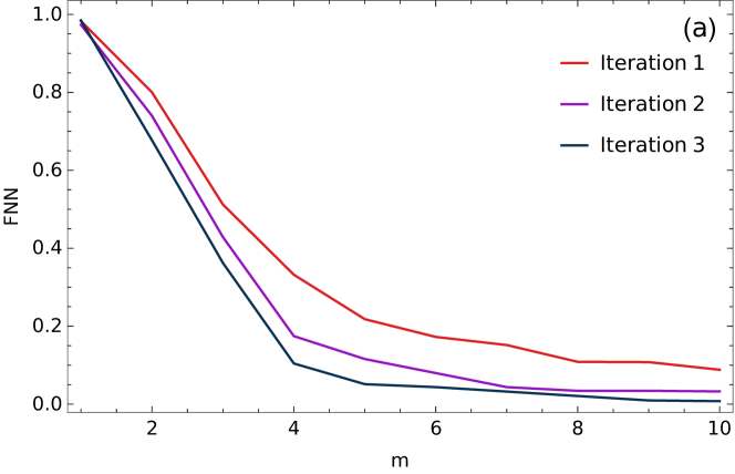
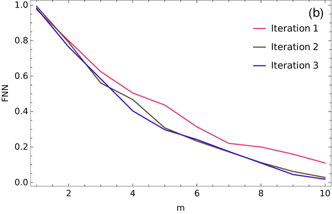
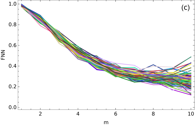
Figure 1: The FNN plot for the logarithmic LC of 3C 279. (a) The knee at $m\simeq 4-5$ indicates the most appropriate embedding dimension; the value $\tau=3$ was used. (b) One can not see such a sharp bending when was set to the delay value $\tau=9$. (c) The lack of a sharp bending is also evident in case of the surrogates.

4.2 Time delay $\tau$

After testing different values of $\tau$ for the phase-space reconstruction and the LEs, we came to the conclusion that various $\tau$ values lead to dramatically different results. MI yielded in general $\tau<15$. The same range of $\tau$ was implied from the ACF, although often the particular values were inconsistent. Fig. 2 shows illustrative plots of MI and ACF. By investigating the phase-space reconstructions and the resulting mLEs, we settled using the values $\tau=3$ and $\tau=8$ as representative.

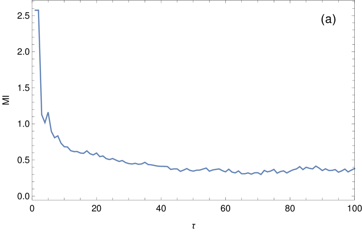
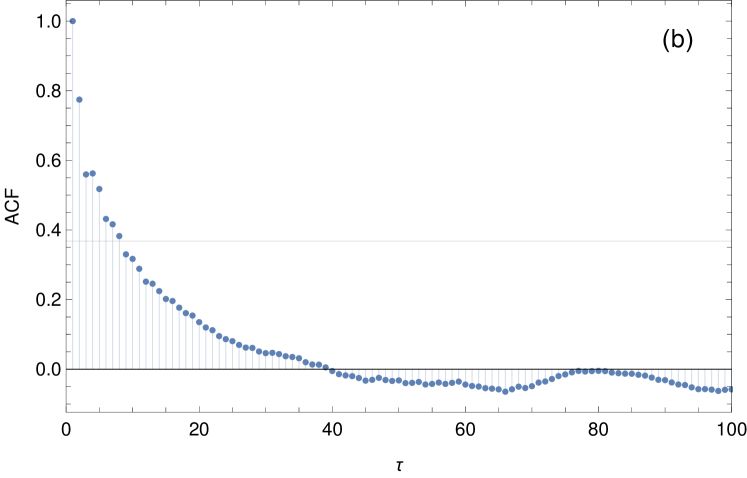
Figure 2: Estimation of the delay $\tau$. (a) The MI has its first local minimum at $\tau=3$. (b) The ACF drops below $1/{\rm e}$ at $\tau=8$.

4.3 Phase-space reconstruction

With the obtained values of $m$ and $\tau$, one can in principle produce a phase-space reconstruction of the trajectory according to Eq. (1). However, for obvious reasons, illustrating graphically the resulting 4- or 5-dimensional trajectory is impossible. For display purposes only, a representation with $\tau=3$ and $\tau=8$ in a 3-dimensional space is displayed in Fig. 3, together with a typical exemplary reconstruction of one of the surrogates.

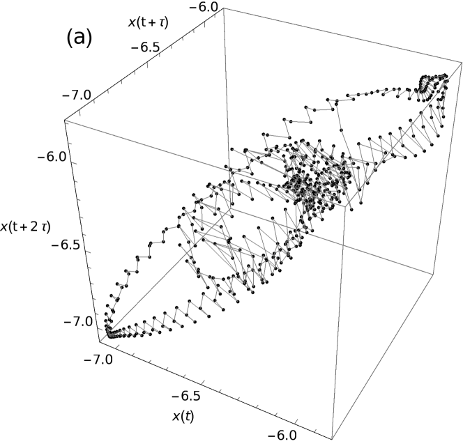
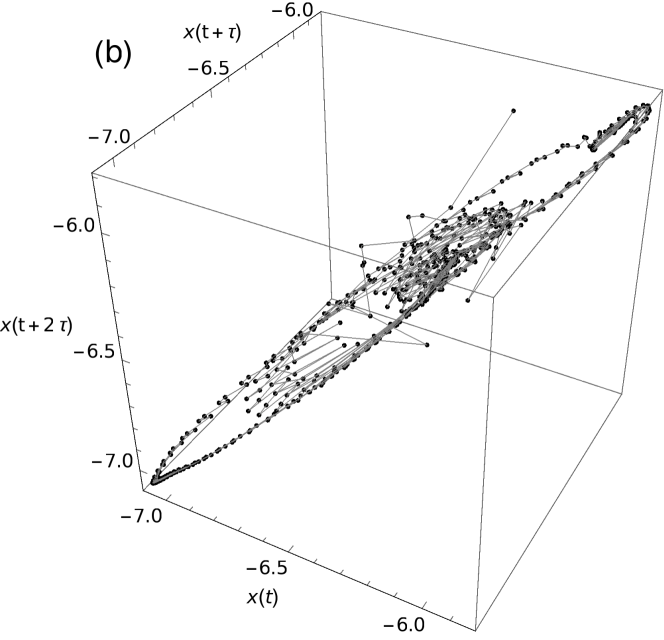
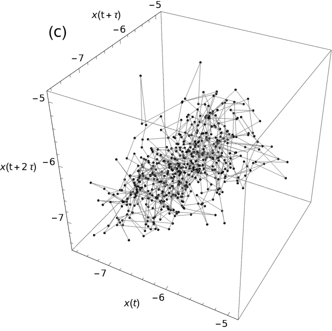
Figure 3: A 3-dimensional phase-space reconstruction of 3C 279. These are projections of the underlying 5-dimensional trajectories. (a) The delay $\tau=8$ was used. (b) In this case $\tau=3$. The topology is still similar. (c) A reconstruction of surrogates. Any structure was destroyed.

4.4 Maximal Lyapunov exponent

Utilizing the obtained values of $m$ and $\tau$, we eventually attempted to constrain the mLE. In Fig. 4, the stretching factors $S(n)$ are depicted for the logarithmic LC itself, as well as for a representative example of a surrogate. As mentioned in Sect. 3.5, in case of chaos three regions should be clearly visible: a sharp increase for very small $n$, followed by a linear section, and finally a plateau. None of these parts are present in Fig. 4(a), also no such features are present in any of the surrogates (cf. Fig. 4(b)). Such results were arrived at for all 11 blazars in our sample.

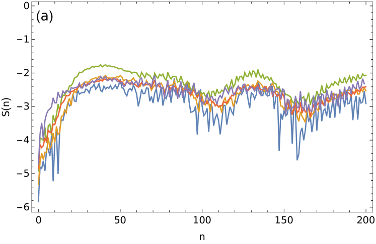
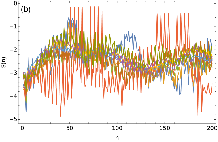
Figure 4: The stretching factors $S(n)$ of (a) 3C 279 and (b) a representative surrogate. In both cases there is no unambiguous linear increase. Different colors correspond to different embedding dimensions $m$.

4.5 Correlation dimension

We constructed a plot of $d_{C}$ as a function of $m$, which is presented in Fig. 5, as means of comparing with other works that utilized this method. In case of a chaotic system a linear increase followed by a plateau should be seen. The analysis of 3C 279 (Fig. 5 (a)) did not provide evidence of chaotic behavior of the system. The plot of the surrogate data in Fig. 5 (b) does not exhibit a plateau part as well. This observation applies to all 11 blazars considered herein.

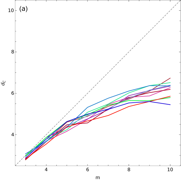
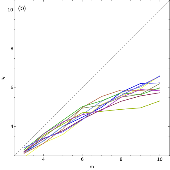
Figure 5: Correlation dimension $d_{C}$ for 3C 279 of (a) the logarithmic LC, and (b) of one of the surrogates. In both plots there is no clear plateau.

5 Discussion

Finding low-dimensional chaos in a phenomenon with not well constrained physics is of great importance, since it provides information about the complexity of the underlying laws governing its occurrence (Seymour & Lorimer, 2013; Bachev et al., 2015). This in particular refers to blazar LCs, in which no unambiguous signs of chaos have been detected. Indeed, the analyses presented herein also did not give the slightest hints allowing to suspect the presence of chaos in any of the 11 objects examined. We displayed here the results corresponding to 3C 279; the other 10 blazars yielded very similar outcomes.

In principal, the behavior of a dynamical system can be described by a set of first-order ordinary differential equations. Such system can be directly investigated to uncover the structure of the phase space and to characterize its dynamical properties. Attractors, their fractal dimensions, Lyapunov exponents, etc. can be easily estimated, and their properties can be studied analytically, semi-analytically, and numerically. However, the underlying equations in most cases of real-world dynamical systems, such as blazar LCs, are unknown. Hence the detection of chaos, or lack of thereof, is a notoriously difficult task, especially in cases when the time series are relatively short and contaminated by observational noise. Noisy data can hinder the detection of chaos; moreover, high-dimensional chaos can be disguised as randomness. Bachev et al. (2015) argued that in the single-zone model there are only a handful of parameters that control the emission, which is governed by the Fokker-Planck (continuity) equation. However, if the radiation mechanism, and subsequently the variability of blazars, can indeed be accurately described by the (partial differential) continuity equation with some appropriate injection term (Stawarz & Petrosian, 2008; Finke & Becker, 2014, 2015; Chen et al., 2016), then the dynamical system is considered to be infinite-dimensional. While chaos can be present in infinite-dimensional systems (e.g. delayed systems; Wernecke et al. 2019), its detection in astronomical LCs need not be unambiguously identifiable with the standard tools, most commonly applied with a discovery of low-dimensional chaos in mind—especially when the details of the fundamental dynamical processes remain unknown, and the time series is not extremely long.

On the other hand, if the radiation is influenced by turbulence in the jets, e.g. by chaotic magnetic flows caused by plasma instabilities, there might be instances in which the behavior of the system settles on some low-dimensional attractor. Therefore, further search for chaos in high-quality (multiwavelength) data gathered by next-generation space instruments, like the James Webb Space Telescope (Gardner et al., 2006), can be expected to give a more definite answer. A uniform, rigorous analysis, in the spirit presented herein, of the already abundantly available optical data from the Kepler space telescope (Smith et al., 2018) is also called for.

6 Conclusions

The aim of this paper was to search for evidence of low-dimensional chaos in $\gamma$-ray LCs of 11 blazars, i.e. five BL Lacs and six FSRQs. Data from Fermi-LAT (10-year-long LCs with a 7-day binning) were investigated using the phase-space reconstruction via embedding dimension $m$ and time delay $\tau$, with the goal of eventually constraining the mLE (if positive) and correlation dimension $d_{C}$.

All analyses implied no signs of chaos for all 11 blazars. Therefore, the underlying physical processes that give rise to the observed variability are either truly stochastic (Tavecchio et al., 2020), or are governed by high-dimensional (possibly infinite-dimensional as well) chaos that can resemble randomness.

Data Availability

The data underlying this article will be shared on reasonable request to the authors.

References

- Abdo et al. (2010) Abdo A. A., et al., 2010, ApJ, 715, 429
- Abdollahi et al. (2020) Abdollahi S., et al., 2020, ApJS, 247, 33
- Akiyama et al. (2016) Akiyama K., Stawarz Ł., Tanaka Y. T., Nagai H., Giroletti M., Honma M., 2016, ApJ, 823, L26
- Atwood et al. (2009) Atwood W. B., et al., 2009, ApJ, 697, 1071
- Bachev et al. (2015) Bachev R., Mukhopadhyay B., Strigachev A., 2015, A&A, 576, A17
- Böttcher et al. (2012) Böttcher M., Harris D. E., Krawczynski H., 2012, Relativistic Jets from Active Galactic Nuclei
- Cecconi et al. (2010) Cecconi F., Cencini M., Vulpiani A., 2010, Chaos: from Simple Models to Complex Systems. World Scientific, Singapore
- Chen et al. (2016) Chen X., Pohl M., Böttcher M., Gao S., 2016, MNRAS, 458, 3260
- Costamante et al. (2001) Costamante L., et al., 2001, A&A, 371, 512
- Eckmann & Ruelle (1992) Eckmann J. P., Ruelle D., 1992, Physica D Nonlinear Phenomena, 56, 185
- Finke & Becker (2014) Finke J. D., Becker P. A., 2014, ApJ, 791, 21
- Finke & Becker (2015) Finke J. D., Becker P. A., 2015, ApJ, 809, 85
- Fraser & Swinney (1986) Fraser A. M., Swinney H. L., 1986, Phys. Rev. A, 33, 1134
- Gardner et al. (2006) Gardner J. P., et al., 2006, Space Sci. Rev., 123, 485
- Grassberger & Procaccia (1983) Grassberger P., Procaccia I., 1983, Physica D Nonlinear Phenomena, 9, 189
- Grassberger et al. (1993) Grassberger P., Hegger R., Kantz H., Schaffrath C., Schreiber T., 1993, Chaos, 3, 127
- Hanslmeier et al. (2013) Hanslmeier A., et al., 2013, A&A, 550, A6
- Hegger & Kantz (1999) Hegger R., Kantz H., 1999, Phys. Rev. E, 60, 4970
- Hegger et al. (1999) Hegger R., Kantz H., Schreiber T., 1999, Chaos, 9, 413
- Kantz & Schreiber (2004) Kantz H., Schreiber T., 2004, Nonlinear Time Series Analysis
- Kennel et al. (1992) Kennel M. B., Brown R., Abarbanel H. D. I., 1992, Phys. Rev. A, 45, 3403
- Kidger et al. (1996) Kidger M. R., Gonzalez-Perez J. N., Sadun A., 1996, in Miller H. R., Webb J. R., Noble J. C., eds, Astronomical Society of the Pacific Conference Series Vol. 110, Blazar Continuum Variability. p. 123
- Kodba et al. (2005) Kodba S., Perc M., Marhl M., 2005, EUROPEAN JOURNAL OF PHYSICS Eur. J. Phys, 26, 205
- Lehto et al. (1993) Lehto H. J., Czerny B., McHardy I. M., 1993, MNRAS, 261, 125
- Lichtenberg & Lieberman (1992) Lichtenberg A. J., Lieberman M. A., 1992, Regular and Chaotic Dynamics. Springer, New York
- Mandelbrot (1983) Mandelbrot B., 1983, The Fractal Geometry of Nature. W. H. Freeman and Company, New York
- Mannattil et al. (2016) Mannattil M., Gupta H., Chakraborty S., 2016, ApJ, 833, 208
- Misra et al. (2004) Misra R., Harikrishnan K. P., Mukhopadhyay B., Ambika G., Kembhavi A. K., 2004, ApJ, 609, 313
- Oprisan et al. (2015) Oprisan S., Lynn P., Tompa T., Lavin A., 2015, Frontiers in Computational Neuroscience, 9, 125
- Padovani (2017) Padovani P., 2017, Nature Astronomy, 1, 0194
- Pascual-Granado et al. (2015) Pascual-Granado J., Garrido R., Suárez J. C., 2015, A&A, 575, A78
- Provenzale et al. (1994) Provenzale A., Vio R., Cristiani S., 1994, ApJ, 428, 591
- Ruelle (1990) Ruelle D., 1990, Proceedings of the Royal Society of London Series A, 427, 241
- Sadun (1996) Sadun A., 1996, in Miller H. R., Webb J. R., Noble J. C., eds, Astronomical Society of the Pacific Conference Series Vol. 110, Blazar Continuum Variability. p. 86
- Seymour & Lorimer (2013) Seymour A. D., Lorimer D. R., 2013, MNRAS, 428, 983
- Shishikura (1998) Shishikura M., 1998, Annals of Mathematics, 147, 225
- Smith et al. (2018) Smith K. L., Mushotzky R. F., Boyd P. T., Malkan M., Howell S. B., Gelino D. M., 2018, ApJ, 857, 141
- Stawarz & Petrosian (2008) Stawarz Ł., Petrosian V., 2008, ApJ, 681, 1725
- Takens (1981) Takens F., 1981, Detecting strange attractors in turbulence. p. 366, doi:10.1007/BFb0091924
- Tarnopolski (2015) Tarnopolski M., 2015, Ap&SS, 357, 160
- Tarnopolski et al. (2020) Tarnopolski M., Żywucka N., Marchenko V., Pascual-Granado J., 2020, The Astrophysical Journal Supplement Series, 250, 1
- Tavecchio et al. (2020) Tavecchio F., Bonnoli G., Galanti G., 2020, MNRAS, 497, 1294
- The Fermi-LAT collaboration (2020) The Fermi-LAT collaboration 2020, ApJS, 247, 33
- Theiler et al. (1992) Theiler J., Eubank S., Longtin A., Galdrikian B., Doyne Farmer J., 1992, Physica D Nonlinear Phenomena, 58, 77
- Urry & Padovani (1995) Urry C. M., Padovani P., 1995, PASP, 107, 803
- Uttley et al. (2005) Uttley P., McHardy I. M., Vaughan S., 2005, MNRAS, 359, 345
- Wernecke et al. (2019) Wernecke H., Sándor B., Gros C., 2019, Physics Reports, 824, 1
- Wolf et al. (1985) Wolf A., Swift J. B., Swinney H. L., Vastano J. A., 1985, Physica D Nonlinear Phenomena, 16, 285
- Wood et al. (2017) Wood M., Caputo R., Charles E., Di Mauro M., Magill J., Perkins J. S., Fermi-LAT Collaboration 2017, in 35th International Cosmic Ray Conference (ICRC2017). p. 824 (arXiv:1707.09551)