Cost-Efficient Online Hyperparameter Optimization

Abstract

Recent work on hyperparameters optimization (HPO) has shown the possibility of training certain hyperparameters together with regular parameters. However, these online HPO algorithms still require running evaluation on a set of validation examples at each training step, steeply increasing the training cost. To decide when to query the validation loss, we model online HPO as a time-varying Bayesian optimization problem, on top of which we propose a novel costly feedback setting to capture the concept of the query cost. Under this setting, standard algorithms are cost-inefficient as they evaluate on the validation set at every round. In contrast, the cost-efficient GP-UCB algorithm proposed in this paper queries the unknown function only when the model is less confident about current decisions. We evaluate our proposed algorithm by tuning hyperparameters online for VGG and ResNet on CIFAR-10 and ImageNet100. Our proposed online HPO algorithm reaches human expert-level performance within a single run of the experiment, while incurring only modest computational overhead compared to regular training.

Keywords: Bayesian Optimization, Hyperparameter Tuning, Gaussian Process

1 Introduction

Training deep neural networks involves a large number of hyperparameters, many of them found through repetitive trial-and-error. Often the results are very sensitive to the selection of hyperparameters and researchers typically follow classic “cookbooks” with many of their hyperparameters copied from the predecessor models. Hyperparameter optimization (HPO) (Hutter et al., 2011; Snoek et al., 2015; Jamieson and Talwalkar, 2016) could potentially save much time from grid search procedures performed in nested loops; however, repetitive experiments on the order of hundreds are still required, which makes applying HPO prohibitively expensive in practice.

Recent advances in meta-optimization (Lorraine and Duvenaud, 2018; MacKay et al., 2019) have shown that one can actually tune certain hyperparameters, e.g., data augmentation, dropout, example weighting, entirely online throughout the training of the main model parameters, by constantly inspecting at the validation loss. While this means that the training job only needs to be launched once, the cost of each training step rises sharply: to learn the hyperparameters, one has to take a gradient step from the reward signals obtained by evaluating on a separate set of validation examples to the hyperparameters. Depending on the size of the validation set, this can make the training time several times longer.

Ultimately, the goal is to design an online HPO algorithm that is efficient in terms of computation cost that arises from validation loss evaluations, i.e., whenever the algorithm queries for “ground-truth” of validation loss. Towards building such an algorithm, we model the environment as a time-varying Bayesian Optimization (BO) problem with unknown time-varying reward/objective. In contrast with the standard BO setting, we require the agent to pay a certain cost to observe the reward every time it decides to query the unknown function. In this paper, we propose a time-varying cost-efficient GP-UCB (Srinivas et al., 2010; Bogunovic et al., 2016) algorithm, and provide kernel-based regret guarantees. Our algorithm makes use of a Gaussian process (GP) model to quantify uncertainty in the estimates and cost-efficient query rule. Based on this rule, the algorithm queries the unknown objective only in rounds when it is ”less” confident in its decision.

We verify the effectiveness of our proposed algorithm empirically by tuning hyperparameters of large scale deep networks. First, we automatically adjust the tuning schedules of self-tuning networks (MacKay et al., 2019) on CIFAR-10 (Krizhevsky et al., 2009). Second, we optimize data augmentation parameters of a state-of-the-art unsupervised contrastive representation learning algorithm (Chen et al., 2020) on ImageNet100 (Deng et al., 2009). We show that with modest computation overhead compared to regular training, one can achieve the same or better performance compared to baselines that have been extensively tuned by human experts.

To summarize, the contributions in this paper are as follows: (1) We introduce a novel costly feedback setting for BO to model the evaluation cost for online HPO; (2) We propose a cost-efficient GP-UCB algorithm with kernel-based theoretical guarantees for time-varying BO with costly feedback; (3) We demonstrate the effectiveness of our method in tuning hyperparameters for modern deep networks in two challenging tasks.

2 Related Work

Bayesian optimization (BO):

BO is a popular framework for optimizing an unknown objective function from point queries that are assumed to be costly (Shahriari et al., 2015). Besides the standard problem formulation (Srinivas et al., 2010), different works have considered various settings including contextual setting (Krause and Ong, 2011), batch and parallel setting (Desautels et al., 2014), optimization under budget constraints (Lam et al., 2016) and robust optimization (Bogunovic et al., 2018). Of particular interest to our work are time-varying BO methods (Bogunovic et al., 2016; Imamura et al., 2020) that consider objectives that vary with time. In Bogunovic et al. (2016), the authors consider time variations that follow a simple Markov model. Their proposed algorithm TV-GP-UCB comes with the model-based forgetting mechanism and attains regret bounds that jointly depend on the time horizon and rate of function variation. In this work, we consider the same time-varying model but in the setting of sparse observations. That is, while previous works have focused on the setting where observations are received at every time step, our goal is to optimize an unknown time-varying objective subject to a specified budget constraint.

Hyperparameter Optimization (HPO):

There are three mainstream frameworks in HPO: model-free, model-based and gradient-based approaches. Specifically, grid search, random search (Bergstra and Bengio, 2012) and its extensions (e.g., successive halving (Jamieson and Talwalkar, 2016) and Hyperband (Li et al., 2017)) are standard model-free HPO methods that ignore the structure of the problem and model. In contrast, BO (Hutter et al., 2011; Bergstra et al., 2011; Snoek et al., 2012, 2015) is a common model-based approach that aims to model the conditional probability of performance given the hyperparameters and a dataset. Other assumptions such as learning curve behavior (Swersky et al., 2014; Klein et al., 2017b; Nguyen et al., 2019) and computational cost (Klein et al., 2017a) are taken into account in BO to avoid learning from scratch every time. However, both model-free and model-based approaches involve repetitive trial-and-error processes that are very expensive in practice. An alternative gradient-based solution is to cast HPO as a bilevel optimization problem and take gradients with respect to the hyperparameters. Since unrolling the whole learning trajectories is prohibitively expensive, researchers usually consider a biased several-step look-ahead approximation (Domke, 2012; Luketina et al., 2016; Franceschi et al., 2018) or the implicit function theorem (Larsen et al., 1996; Pedregosa, 2016; Lorraine et al., 2019; Bertrand et al., 2020) to obtain the gradients. To further improve the efficiency of HPO, recent works (Lorraine and Duvenaud, 2018; MacKay et al., 2019) utilize hypernetworks (Ha et al., 2017) to approximate the inner optimization loop and a held-out validation set to collect reward signals. Instead of constantly evaluating the validation loss, which brings remarkable computation overhead, this work propose a cost-efficient evaluation rule, and emprirically demonstrates it effectiveness in the real HPO tasks.

3 Bayesian Optimization with Costly Feedback

Recent online HPO algorithms require to obtain reward signals constantly by evaluating the metrics such as performance gain on the validation set, drastically increasing the training cost. Motivated by this observation, we model HPO as a time-varying Bayesian optimization (BO) problem where the unknown function is treated as the reward signals obtained through subsequent evaluations. To capture the evaluation cost induced by observing the rewards, we introduce a novel costly feedback setting that allows the agent to decide, at every round, whether to receive the observation. In turn, the agent is required to pay a certain cost whenever it receives feedback.

3.1 Problem Setup

We aim to sequentially optimize an unknown objective function $f_{t}(x):\mathcal{D}\times\mathcal{T}\rightarrow\mathbb{R}$ defined on composite space $\mathcal{X}=\mathcal{D}\times\mathcal{T}$, where $\mathcal{D}$ is the finite input domainand $\mathcal{T}=\{1,2,\dots,T\}$ represents the time domain. At each round $1\leq t\leq T,t\in\mathbb{N}$, the agent decides upon a data point $x_{t}$. After selecting the point $x_{t}$, it has the option to decide whether to receive the feedback by interacting with $f_{t}$. If the agent chooses to observe the feedback, then it receives a noisy observation $y_{t}=f_{t}(x)+z_{t}$, where $z_{t}$ is assumed to be independently sampled from a Gaussian distribution $\mathcal{N}(0,\sigma^{2})$. Let $\mathcal{S}_{t}^{n}=\{(x_{h(i)},y_{h(i)},i)\}_{i=1}^{n}$ denote the data obtained through $n$ observations till round $t$. Here $h(i)$ denotes the mapping function that records the round at which the agent observes the $i$-th data point. The agent then chooses its next point $x_{t+1}$ based on the previously collected data $\mathcal{S}_{t}^{n}$. If the agent decides to query the unknown function at round $t$, then it needs to pay a cost $c_{t}$. We let $c_{t}=1$ if the feedback $y_{t}$ is received at round $t$, and otherwise $c_{t}=0$. We define the cumulative cost as $C_{T}=\sum_{t=1}^{T}c_{t}$ that records the total number of queries within $T$ rounds.

Connection to online HPO:

In this paper, online HPO is modeled as the time-varying BO with costly feedback – hyperparameter configurations $x_{t}$ are selected sequentially to maximize the reward signals $f_{t}(x)$. Since evaluation on the validation set is expensive, the agent is allowed to skip the evaluation or pay a certain cost $c_{t}$ to see the reward.

To measure the performance of algorithms, the regret for $t$-th round is defined as $r_{t}=\max_{x\in\mathcal{D}}f_{t}(x)-f_{t}(x_{t})$. The cumulative regret $R_{T}$ is the sum of instantaneous regrets $R_{T}=\sum_{t=1}^{T}r_{t}$. Furthermore, we define the cumulative loss as $L_{T}=R_{T}+C_{T}$ to balance between regret and cost. We note that if an agent queries the unknown objective function at each time step, we recover the standard time-varying BO setting Bogunovic et al. (2016).

4 Cost-Efficient GP-UCB Algorithm

Since the reward signals for online HPO vary as the learning proceeds, and similar hyperparameter configurations lead to similar performance, we consider using a time-varying Gaussian process (GP) to model the objective function $f_{t}$. Consequently, we start this section by studying the behavior of time-varying GP models with sparse observations. We then propose a novel cost-efficient algorithm and study its theoretical performance. We defer all the analysis to the supplementary material.

4.1 Time-varying Gaussian Process Model

We use a spatio-temporal GP to model the underlying function $f_{t}$. The smoothness properties of $f_{t}$ are depicted by a composite kernel function (Bogunovic et al., 2016; Imamura et al., 2020): $k=k_{\mathrm{space}}\otimes k_{\mathrm{time}}$, where $k_{\mathrm{space}}:\mathcal{D}\times\mathcal{D}\rightarrow\mathbb{R}^{+}$ and $k_{\mathrm{time}}:\mathcal{T}\times\mathcal{T}\rightarrow\mathbb{R}^{+}$ are spatial and temporal kernels; $(k_{\mathrm{space}}\otimes k_{\mathrm{time}})((x,t),(x^{\prime},t^{\prime})):=k_{\mathrm{space}}(x,x^{\prime})\cdot k_{\mathrm{time}}(t,t^{\prime})$. Following Bogunovic et al. (2016), we consider the following transition relation of the underlying function: $f_{t+1}(x)=\sqrt{1-\epsilon}f_{t}(x)+\sqrt{\epsilon}g_{t+1}(x)$, where $g_{t}$ is sampled from a GP with a mean function $\mu$ and a kernel function $k$, i.e., $g_{t}\sim\mathcal{G}\mathcal{P}(\mu,k)$; $\epsilon\in[0,1]$ is the forgetting rate that constrains the variation of the function. This particular Markov model maps to the following exponential temporal kernel as shown in Bogunovic et al. (2016): $k_{\mathrm{time}}\left(\tau,\tau^{\prime}\right)=(1-\epsilon)^{\frac{\left|\tau-\tau^{\prime}\right|}{2}}.$

Given observed data points $\mathbf{x}_{t}^{n}=\{x_{h(1)},\dots,x_{h(n)}\}$ and $\mathbf{y}_{t}^{n}=\{y_{h(1)},\dots,y_{h(n)}\}$, the posterior over $f$ is a GP with mean $\tilde{\mu}_{t}(x)$, covariance $k_{t}(x,x^{\prime})$ and variance $\tilde{\sigma}_{t}^{2}(x)=k_{t}(x,x)$:

$$\tilde{\mu}_{t}(x) =\widetilde{\mathbf{k}}_{t}^{n}(x)^{T}\left(\widetilde{\mathbf{K}}_{t}^{n}+\sigma^{2}\mathbf{I}_{t}^{n}\right)^{-1}\mathbf{y}_{t}^{n},$$ (1)

$$k_{t}(x,x^{\prime}) =k(x,x^{\prime})-\widetilde{\mathbf{k}}_{t}^{n}(x)^{T}\left(\widetilde{\mathbf{K}}_{t}^{n}+\sigma^{2}\mathbf{I}_{t}^{n}\right)^{-1}\widetilde{\mathbf{k}}_{t}^{n}(x^{\prime}),$$ (2)

where $\widetilde{\mathbf{K}}_{t}^{n}=\mathbf{K}_{t}^{n}\circ\mathbf{D}_{t}^{n}$, with $\mathbf{D}_{t}^{n}=\left[(1-\epsilon)^{|h(i)-h(j)|/2}\right]_{i,j=1}^{n}$, and $\tilde{\mathbf{k}}_{t}^{n}(x)=\mathbf{k}_{t}^{n}(x)\circ\mathbf{d}_{t}^{n}$ with $\mathbf{d}_{t}^{n}=$ $\left[(1-\epsilon)^{(t+1-h(i))/2}\right]_{i=1}^{t}$. Here $\mathbf{K}_{t}^{n}=$ $\left[k\left(x_{i},x_{j}\right)\right]^{n}_{i,j=1}$, $\mathbf{k}_{t}^{n}(x)=\left[k\left(x_{i},x\right)\right]_{i=1}^{n}$, $\circ$ is the Hadamard product, and $\mathbf{I}_{t}^{n}$ is the $n\times n$ identity matrix.

One key challenge in BO is to balance the exploration-exploitation tradeoffs rigorously. Various works (e.g., Srinivas et al. (2010); Bogunovic et al. (2016)) have focused on the upper-confidence bound (UCB) rule that selects points by maximizing a linear combination of posterior mean and variance. In this paper, our focus is also on the UCB rule due to its strong theoretical guarantees and empirical performance. In what follows, we let $\operatorname*{ucb}_{t}(x):=\tilde{\mu}_{t}(x)+\beta_{t+1}^{1/2}\tilde{\sigma}_{t}(x)$, where $\{\beta_{t}\}_{t=1}^{T}$, each $\beta_{t}\in\mathbb{R_{+}}$, is a non-decreasing sequence of exploration parameters, selected as Bogunovic et al. (2016), such that (w.h.p.) $\operatorname*{ucb}_{t}(x)$ is a valid upper confidence bound on $f_{t}(x)$ for every $x$ and $t$.

4.2 Strategies for Querying Feedback

In BO with costly feedback, there are two decisions for the agent to make at every round: 1) where to evaluate the unknown objective; 2) whether to receive the feedback (and consequently incur cost). In this section, we focus on the latter problem. To minimize regret while reducing the query cost, we propose two strategies for the query allocation.

Querying with Bernoulli Sampling Schedule:

A simple and model-agnostic method for our problem is to query the objective function according to a fixed probability. Specifically, we query the feedback based on a Bernoulli random variable $\operatorname*{Ber}(B/T)$, which guarantees that the algorithm receives in expectation $B$ observations of $y_{t}$.

Leveraging Uncertainty Information from GP:

Although the Bernoulli strategy defined above can reduce the query cost, it does not leverage any knowledge from the GP model. As a consequence, in practice, there is often a significant performance loss compared to standard algorithms with full observations. To overcome this difficulty, we propose a cost-efficient query rule that automatically assesses the uncertainty of the current decision for time-varying GP-UCB (Bogunovic et al., 2016) and its variants.

On a high level, the agent aims to maintain informative queries but skip uninformative ones to save the query cost. Hence, we consider the following cost-efficient query rule: the agent only queries the feedback when the following condition satisfies:

$$\mathbb{P}\left(\hat{y}_{t}({x_{t}})>\hat{y}_{t}({x})\right)<\kappa,\ \exists x\in\mathcal{D}\setminus\{x_{t}\},$$

where $\hat{y}_{t}(x)$ is the posterior predictive estimation of the unknown objective at point $x$, which is a random variable distributed according to $\mathcal{N}\left(\tilde{\mu}_{t}(x),\tilde{\sigma}^{2}_{t}(x)\right)$. The analytic solution to $\mathbb{P}\left(\hat{y}_{t}({x_{t}})>\hat{y}_{t}({x})\right)<\kappa$, as well as the analysis of the choices of $\kappa$ are provided in Appendix A. This rule explicitly encourages receiving feedback when the agent is less confident in distinguishing the best candidate. The intuition behind this rule is to skip querying $f_{t}$ when the selected $x_{t}$ leads to “small” regret.

4.3 Cost-Efficient GP-UCB Algorithm

We integrate the two strategies for querying feedback in time-varying GP-UCB model and obtain two algorithms for our costly feedback setting. Specifically, we give the cost-efficient algorithm (CE-GP-UCB) that leverages the uncertainty information from GP in Algorithm 1. Our algorithm selects the points with largest UCB at every round (Line 4) but only observes the feedback $y_{t}$ when the when the model is most uncertain (Line 5). Note that the query strategy can be replaced by Bernoulli sampling strategy to consume the budget $B$ as introduced in Sec 4.2.

When no feedback is received (Line 9), there is no update of the GP model; however, due to the time-varying nature, the model will be less confident about the estimation for the candidates thus the posterior variance will increase.

Remark:

Note that if the candidates are close to each other (e.g., quantized candidates for continuous variables), the model will never be confident in its current decision since the UCB of best and second-best candidates are very close. In other words, the cost-efficient query rule (Line 4 in Algorithm 1) will continuously be activated. However it is less informative to query the feedback for two close candidates within one mode. Therefore, in practice, we first find the local optima of the UCB function and their corresponding data points, then deploy the cost-efficient query rule for these local optima.

Algorithm 1 CE-GP-UCB

1:Input Domain $\mathcal{D}$, total rounds $T$, GP prior $\left(\tilde{\mu}_{0},\tilde{\sigma}_{0},k\right)$, forgetting rate $\epsilon$, user-specific confidence threshold $\kappa$

2:Initialize observation set $\mathcal{S}_{0}^{0}=\emptyset$, number of interactions $n=0$.

3:for $t=1,2,\cdots,T$ do

4:    Choose $x_{t}=\arg\max_{x\in\mathcal{D}}\tilde{\mu}_{t-1}(x)+\sqrt{\beta_{t}}\tilde{\sigma}_{t-1}(x)$ $\triangleright$ Select points according to UCB rule

5:    if $\mathbb{P}\left(\hat{y}_{t}({x_{t}})>\hat{y}_{t}({x})\right)<\kappa$, $\exists x\in\mathcal{D}\setminus\{x_{t}\}$ then $\triangleright$ Cost-efficient query strategy

6:         Receive feedback $y_{t}=f_{t}\left(x_{t}\right)+z_{t}$, $n\leftarrow n+1$ $\triangleright$ Interact with $f_{t}$ and receive feedback

7:         Add $(x_{t},y_{t},t)$ to observation set: $\mathcal{S}_{t}^{n+1}=\mathcal{S}_{t-1}^{n}\cup{(x_{t},y_{t},t)}$

8:         Perform Bayesian update to obtain $\tilde{\mu}_{t}$ and $\tilde{\sigma}_{t}$

9:    else $\tilde{\mu}_{t}=\tilde{\mu}_{t-1},\tilde{\sigma}_{t}=\tilde{\sigma}_{t-1}$, $\mathcal{S}_{t}^{n}=\mathcal{S}_{t-1}^{n}$ $\triangleright$ Do not observe feedback

10:    end if

11:end for

5 Experiments

We thoroughly evaluate the proposed algorithm on both synthetic data and practical online hyperparameter optimization problems: (1) tuning schedules for self-tuning networks (STN MacKay et al. (2019)); (2) data augmentations for unsupervised representation learning (Chen et al., 2020). Extensive experiments show that cost-efficient query rule leads to substantial improvements over simple Bernoulli strategy. We leave extra experimental details in Appendix B.

5.1 Evaluation on Synthetic Data

We follow the same synthetic setting as previous study Bogunovic et al. (2016). Specifically, we used a one-dimensional input domain $\mathcal{D}=[0,1]$ and quantized it into 1,000 uniformly divided points. We generated the time-varying objective functions according to the following Markov model $f_{t+1}(x)=\sqrt{1-\epsilon}f_{t}(x)+\sqrt{\epsilon}g_{t+1}(x)$ under different forgetting rate $\epsilon$, where $g_{t}(x)\sim\mathcal{GP}(0,k)$. We use Matérn3/2 kernel for GP models and set sampling noise variance $\sigma^{2}=0.01$. The time horizon $T$ is set as 500.

Figure 1 shows the trade-off curves between average regret $R_{T}/T$ and query cost $C_{T}$ for different algorithms, where the performance is averaged over 50 independent trials. Specifically, we consider the TV-GP-UCB (Bogunovic et al., 2016), R-GP-UCB (Bogunovic et al., 2016), and its variants with other popular acquisition functions (PI: probability of improvement; EI: expected improvement) with Bernoulli query policy. We observe that our method suffers from a minor regret loss when using 50% query cost ($C_{T}=250$), whereas other baselines with Bernoulli strategy lead to a larger performance loss. We then visualize the final GP models in Figure 2 ($\epsilon=0.03$). In particular, CE-GP-UCB maintains a similar posterior mean and variance for the unknown function compared with TV-GP-UCB with full observations and skips the queries when chosen candidates are close to the optimal ones. By contrast, TV-GP-UCB with Bernoulli strategy skips the queries even when the selected points are far from the optimal ones, thus leading a larger regret.

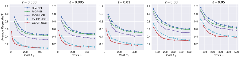
Figure 1: Comparison of trade-off between average regret $R_{T}/T$ and query cost $C_{T}$.

(a) TV-GP-UCB

(b) TV-GP-UCB Ber(0.8)

(c) ours ($\kappa=0.90$)

(d) ours ($\kappa=0.95$)

Figure 2: Visualizations of GP models. The purple points and green points denote the agents’ choices to receive the feedback or not. Data points with darker color mean that they are visited more recently. The blue line (—) and dashed red line (—) indicate the ground truth of unknown objective function and the posterior mean. The gray area denotes the confidence area.

5.2 Self-Tuning Networks

To further study the effectiveness of our algorithm in real applications, we first evaluate the proposed method in adjusting the tuning schedule for self-tuning networks (Lorraine and Duvenaud, 2018) (STN). STN is an online HPO algorithm that uses a hypernetwork (Ha et al., 2017) to approximate the inner loop of bilevel optimization. Standard STN tunes hyperparameters (e.g., dropout, weight-decay and data augmentation) by alternating the following two steps (i.e., train/val=1:1): (1) (training phase) train one mini-batch data on training set; (2) (tuning phase) evaluate one mini-batch data on held-out validation set then backpropagate gradients through the hypernetwork to update hyperparameters. However, we found that STN is sensitive to different tuning schedules and standard “dense tuning” is expensive and sub-optimal.

Table 1: Comparison with conventional MAB algorithms for STN (VGG16 on CIFAR-10).

		$\ell_{val}$	Accval	$\ell_{test}$	Acctest	$T_{total}$
Grid Search		0.421	0.887	0.444	0.879	11.69 $\times$
Ber(0.1)	EXP3.R	0.466	0.841	0.479	0.835	0.93 $\times$
	$\epsilon$-greedy	0.419	0.864	0.438	0.859	0.92 $\times$
	Softmax	0.433	0.854	0.459	0.846	0.93 $\times$
	UCB	0.447	0.869	0.451	0.867	0.94 $\times$
	GP-UCB	0.422	0.877	0.449	0.868	0.96 $\times$
Ber(0.2)	EXP3.R	0.446	0.853	0.455	0.847	1.13 $\times$
	$\epsilon$-greedy	0.401	0.881	0.443	0.873	1.13 $\times$
	Softmax	0.449	0.862	0.480	0.852	1.13 $\times$
	UCB	0.398	0.878	0.421	0.871	1.13 $\times$
	GP-UCB	0.413	0.880	0.439	0.870	1.17 $\times$
CE-GP-UCB ($\kappa=0.7$)		0.390	0.888	0.428	0.881	1.10 $\times$
CE-GP-UCB ($\kappa=0.8$)		0.373	0.892	0.404	0.881	1.21 $\times$

As a consequence, we model STN as a two-armed bandits: “training only” and “tuning + training”. Since tuning one mini-batch data is biased, we define the unknown objective function as the accuracy gain on the whole validation dataset, which is expensive to obtain thus leading a large query cost. We evaluate the proposed approach and other TV bandit algorithms for VGG16 on CIFAR-10. Specifically, we randomly choose 10,000 training images as the validation set, and tune layerwise dropout and data augmentation parameters, following Lorraine and Duvenaud (2018). The network is trained 150 epochs with an initial learning rate 0.1. The learning rate is decayed at 60, 100 and 120 epochs with a decay rate of 0.1.

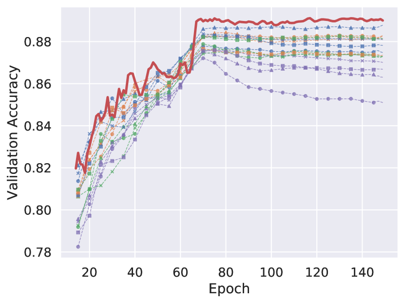
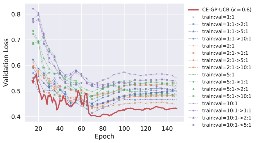
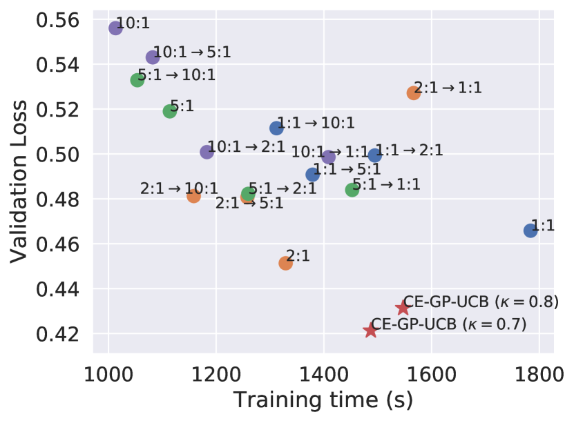
Figure 3: (a) Validation accuracy and & (b) validation loss for STN with different tuning schedules. (c) Trade-offs between validation loss and corresponding training time (excluding querying cost).

We first consider two baselines including static schedules (MacKay et al., 2019) and a simple switching heuristics (e.g., train:val=1:1$\rightarrow$2:1) that occurs at 100 epochs in which the learning rate is decayed. Since smaller learning rate is easier to cause overfitting, we expect to find a better schedule by also decaying the tuning frequency at the late training stage. The dashed lines in Figure 3 (a) & (b) show that the performance of STN is sensitive to varied tuning schedules. As shown in Figure 3 (a) & (b), our approach leads to the best performance in terms of validation accuracy and loss with only a single run of the experiment. In Figure 3 (c), CE-GP-UCB successfully finds an efficient tuning schedule online that saves around 20% training cost meanwhile achieving lower validation loss. Table 1 gives a quantitative comparison between our algorithm and other baselines including grid search and TV bandits algorithms with Bernoulli strategy. After taking account of the cost for evaluation on the validation set, we find that the GP-UCB algorithm with cost-efficient query rule outperforms other baselines on both validation and testing set with modest computation overhead.

5.3 Unsupervised Representation Learning

We evaluate our approach on tuning data augmentations in unsupervised contrastive learning. The goal of unsupervised learning is to learn meaningful representations directly from unlabeled data since acquiring annotations is expensive. SimCLR (Chen et al., 2020) is the state-of-the-art approach that learns representations by maximizing agreement between differently augmented views of the same data example. It is shown in Chen et al. (2020) that the types of data augmentations are critical in learning meaningful representations so researchers conducted extensive ablation study in data augmentations. By contrast, we aim to apply CE-GP-UCB in tuning the probability of randomly applying eight common data augmentations including cropping, color distortion, cutout, flipping horizontally and vertically, rotation, Gaussian blur and gray scale with one single run. We define the accuracy gain (%) on validation set as the costly feedback. The initial probability for applying each data augmentation is set 0.5 and the tuning range is $[0,1.0]$. The forgetting rate $\epsilon$ and $\beta_{t}$ are set as 0.01 and 1.0, respectively. We leave the implementation details of SimCLR in Appendix B.

Table 2: Linear readout performance (ImageNet100 top-1 accuracy) of ResNet50 with different data augmentations.

	Top1 (R10)	Top1 (R100)	Time
Baseline	70.91	73.20	1.00 $\times$
TV-GP-UCB (full)	75.14	77.95	1.97 $\times$
TV-GP-UCB Ber(0.6)	72.15	75.31	1.64 $\times$
CE-GP-UCB ($\kappa=0.9$)	74.80	77.56	1.88 $\times$
CE-GP-UCB ($\kappa=0.8$)	74.77	77.62	1.71 $\times$
CE-GP-UCB ($\kappa=0.7$)	74.58	77.27	1.61 $\times$
Human expert (Chen et al., 2020)	75.00	77.99	-

Table 2 shows the linear readout performance for different models, where the baseline is SimCLR with fixed initial probability (0.5) for eight data augmentations. As shown in Table 2, our method reaches human expert-level performance with one single run of experiment and surpass baseline (no HPO) by a large margin. More importantly, proposed CE-GP-UCB is able to reduce 40% query cost for validation with minor performance loss compared to TV-GP-UCB with full observations; however, TV-GP-UCB with Bernoulli strategy results in a large performance loss. It again verifies proposed cost-efficient query rule is able to successfully maintain the most informative queries and provide an alternative BO solution when resources are limited.

6 Conclusion

Online HPO typically requires constantly evaluating on the validation set and taking gradient steps w.r.t. hyperparameters, resulting in drastically higher training cost. In this paper, we propose a novel costly feedback Bayesian optimization (BO) setting to model the computation cost for querying the reward signals from the validation set. To keep most informative queries and skip less informative ones, we introduce a cost-efficient GP-UCB algorithm that automatically assesses the uncertainty of current GP model. We further verify the effectiveness of our proposed approach with extensive experiments on both synthetic data and large-scale real world online HPO for deep neural networks.

A Choices of Confidence threshold $\kappa$ in CE-GP-UCB

In what follows, we first give an important property induced by no overlapping between the confidence bounds of best candidate $x_{t}$ and the other points $x\in\mathcal{D}\setminus\{x_{t}\}$.

Lemma 1

Let $\delta\in(0,1)$ and $x_{t}=\arg\max_{x\in\mathcal{D}}\tilde{\mu}_{t-1}(x)+\sqrt{\beta_{t}}\tilde{\sigma}_{t-1}(x)$, if $\mathrm{ucb}(x)\leq\mathrm{lcb}(x_{t}),\forall x\in\mathcal{D}\setminus\{x_{t}\}$, then picking $x_{t}$ at round $t$ produces no regret with at least probability $1-\delta$.

Proof [Proof of Lemma 1] From previous literature, we know that, with high probability

$$\left|f_{t}(x)-\tilde{\mu}_{t-1}(x)\right|\leq\beta_{t}^{\frac{1}{2}}\tilde{\sigma}_{t-1}(x).\quad\forall x\in\mathcal{D},\forall t\geq 1$$ (3)

As a result, we have $\tilde{\mu}_{t-1}(x)-\beta_{t}^{\frac{1}{2}}\tilde{\sigma}_{t-1}(x)\leq f_{t}(x)\leq\tilde{\mu}_{t-1}(x)+\beta_{t}^{\frac{1}{2}}\tilde{\sigma}_{t-1}(x)$ $\forall x\in\mathcal{D}$ $\forall t\geq 1$. Let $x^{*}_{t}=\max_{x\in\mathcal{D}}f_{t}(x)$. If $x^{*}_{t}=x_{t}$, then the instantaneous regret $r_{t}=0$. Otherwise,

$$f_{t}(x^{*})-f_{t}(x_{t}) \leq\tilde{\mu}_{t-1}(x^{*}_{t})+\beta_{t}^{\frac{1}{2}}\tilde{\sigma}_{t-1}(x^{*}_{t})-\left(\tilde{\mu}_{t-1}(x_{t})-\beta_{t}^{\frac{1}{2}}\tilde{\sigma}_{t-1}(x_{t})\right)\leq 0$$ (4)

From the definition of $x_{t}^{*}$, we known $f_{t}(x^{*})-f_{t}(x_{t})\geq 0$. So we have picking $x_{t}$ at round t produces no regret with high probability.  

Lemma 1 indicates that if there is no overlapping between the confidence bounds of best candidate $x_{t}$ and the others, the agent can assure that $x_{t}$ is the optimal choice with high probability. As a consequence, if the above condition satisfies, the agent is able to receive no feedback meanwhile resulting in no performance loss at this time. This inspires us to leverage the information that exists in relative magnitudes of posterior mean and variance for the given candidates and obtain the cost-efficient query strategy, which is a loosed condition with a confidence threshold $\kappa\in(0,1)$.

We know $\hat{y}_{t}(x)$ follows the Gaussian distribution $\mathcal{N}(\tilde{\mu}_{t-1}(x),\tilde{\sigma}_{t-1}(x))$. Then we know $\hat{y}_{t}(x_{t})-\hat{y}_{t}(x_{t}^{*})$ follows the distribution

$$\mathcal{N}\left(\tilde{\mu}_{t-1}(x_{t})-\tilde{\mu}_{t-1}(x_{t}^{*}),\sqrt{\tilde{\sigma}^{2}_{t-1}(x_{t})+\tilde{\sigma}^{2}_{t-1}(x_{t}^{*})}\right).$$

As a consequence,

$$1-\Phi\left(-\frac{\tilde{\mu}_{t-1}(x_{t})-\tilde{\mu}_{t-1}(x_{t}^{*})}{\sqrt{\tilde{\sigma}^{2}_{t-1}(x_{t})+\tilde{\sigma}^{2}_{t-1}(x_{t}^{*})}}\right)\geq\gamma_{t},$$ (5)

where $\Phi(\cdot)$ is the CDF of standard Gaussian distribution. To simplify further, we have

$$\tilde{\mu}_{t-1}(x_{t})-\tilde{\mu}_{t-1}(x_{t}^{*}) \geq\Phi^{-1}(\gamma_{t})\sqrt{\tilde{\sigma}^{2}_{t-1}(x_{t})+\tilde{\sigma}^{2}_{t-1}(x_{t}^{*})}$$ (6)

$$\geq\frac{\Phi^{-1}(\gamma_{t})}{\sqrt{2}}\left(\tilde{\sigma}_{t-1}(x_{t})+\tilde{\sigma}_{t-1}(x_{t}^{*})\right).$$ (7)

If $x_{t}^{*}\neq x_{t}$, we have

$$f_{t}(x^{*})-f_{t}(x_{t}) \leq\tilde{\mu}_{t-1}(x^{*}_{t})+\beta_{t}^{\frac{1}{2}}\tilde{\sigma}_{t-1}(x^{*}_{t})-\left(\tilde{\mu}_{t-1}(x_{t})-\beta_{t}^{\frac{1}{2}}\tilde{\sigma}_{t-1}(x_{t})\right)$$ (8)

$$\leq\tilde{\mu}_{t-1}(x^{*}_{t})-\tilde{\sigma}_{t-1}(x^{*}_{t})+\beta_{t}^{\frac{1}{2}}\left(\tilde{\sigma}_{t-1}(x^{*}_{t})+\tilde{\sigma}_{t-1}(x_{t})\right)$$ (9)

$$\leq\left(\beta_{t}^{\frac{1}{2}}-\frac{\Phi^{-1}(\gamma_{t})}{\sqrt{2}}\right)\left(\tilde{\sigma}_{t-1}(x^{*}_{t})+\tilde{\sigma}_{t-1}(x_{t})\right).$$ (10)

Let $\gamma_{t}=\Phi(\sqrt{2}\beta_{t})$, we recover the LCB-UCB rule (free no regret). If $\gamma_{t}<\Phi(\sqrt{2}\beta_{t})$, then the agents suffer from a “small regret” $\left(\beta_{t}^{\frac{1}{2}}-\frac{\Phi^{-1}(\gamma_{t})}{\sqrt{2}}\right)\left(\tilde{\sigma}_{t-1}(x^{*}_{t})+\tilde{\sigma}_{t-1}(x_{t})\right)$.

In practice, we found LCB-UCB rule (Lemma 1) is a very strict rule that might has limited effect in reducing the query cost. For instance, as shown in Table A2, we found LCB-UCB rule is more strict than $\kappa=0.99$.

B Supplementary Experiments

In this section, we provide the details of experimental set-up and supplementary results.

B.1 Evaluation on Synthetic Data

Apart from BO setting where the candidates are correlated (e.g., $k_{\mathrm{space}}$ is SE or Matérn kernels), we consider the finite-arm bandits setting where each arm is assumed independent (i.e., $k_{\mathrm{space}}=I$). Specifically, we consider a three-armed bandit problem where the reward for each arm is sampled from its underlying time varying functions ($\sigma^{2}=0.01$). Specifically, we design three kinds of functions: (1) a sine curve (2) a Gaussian curve, and (3) a piecewise step function, where the time horizon $T=2000$. Figure A1 shows an example of the time-varying functions. We compare with other TV bandits algorithms with Bernoulli sampling policy (Sec 4.2), i.e., $m\sim\operatorname*{Ber}(0.1)$ incorporated, including EXP3.S (Auer et al., 2002b), $\epsilon$-greedy (Kuleshov and Precup, 2000), Softmax (Boltzmann Exploration) (Kuleshov and Precup, 2000), UCB (Auer et al., 2002a) and GP-UCB (Srinivas et al., 2010). We used the RBF kernel in GP models and the parameters (e.g., length scale) for GP are optimized using maximum likelihood. Each experiment is repeated 100 times with different random seeds.

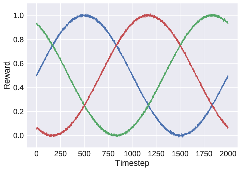
(a) Sine

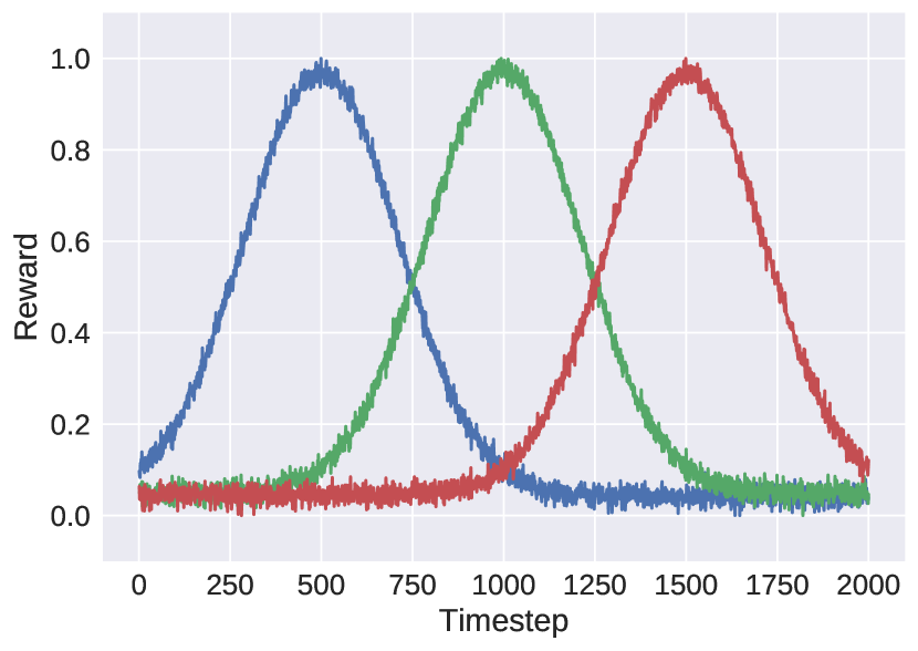
(b) Gaussian

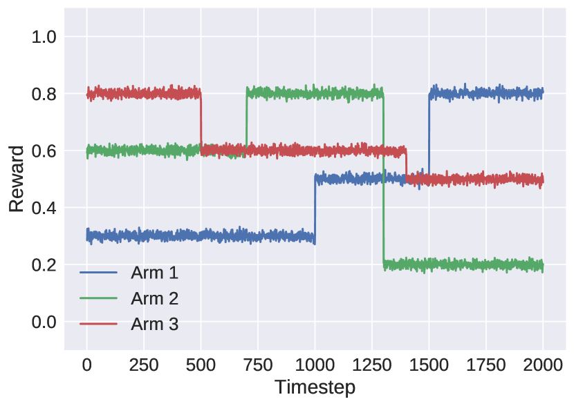
(c) Piecewise

Figure A1: Time-varying functions considered for the synthetic bandit experiments.

Table A1: Comparison of CE-GP-UCB ($\kappa=95\%$) with standard TV bandits algorithms with Bernoulli query strategy on three kinds of synthetic data.

	Sine		Gaussian		Piecewise
	$R_{T}/T$	$C_{T}$	$R_{T}/T$	$C_{T}$	$R_{T}/T$	$C_{T}$
EXP3.S (Auer et al., 2002b)	0.384 $\pm$ 0.036	201 $\pm$ 15	0.257 $\pm$ 0.017	200 $\pm$ 11	0.437 $\pm$ 0.046	201 $\pm$ 14
$\epsilon$-greedy (Kuleshov and Precup, 2000)	0.167 $\pm$ 0.041	198 $\pm$ 14	0.145 $\pm$ 0.026	200 $\pm$ 12	0.196 $\pm$ 0.026	199 $\pm$ 14
Softmax (Kuleshov and Precup, 2000)	0.132 $\pm$ 0.025	199 $\pm$ 13	0.159 $\pm$ 0.032	201 $\pm$ 14	0.256 $\pm$ 0.037	198 $\pm$ 14
UCB (Auer et al., 2002a)	0.084 $\pm$ 0.010	200 $\pm$ 14	0.112 $\pm$ 0.026	201 $\pm$ 15	0.172 $\pm$ 0.042	202 $\pm$ 14
GP-UCB (Srinivas et al., 2010)	0.104 $\pm$ 0.012	200 $\pm$ 14	0.139 $\pm$ 0.025	200 $\pm$ 14	0.122 $\pm$ 0.009	201 $\pm$ 12
CE-GP-UCB	0.017 $\boldsymbol{\pm}$ 0.009	52 $\boldsymbol{\pm}$ 7	0.038 $\boldsymbol{\pm}$ 0.017	53 $\pm$ 20	0.028 $\boldsymbol{\pm}$ 0.002	52 $\boldsymbol{\pm}$ 5

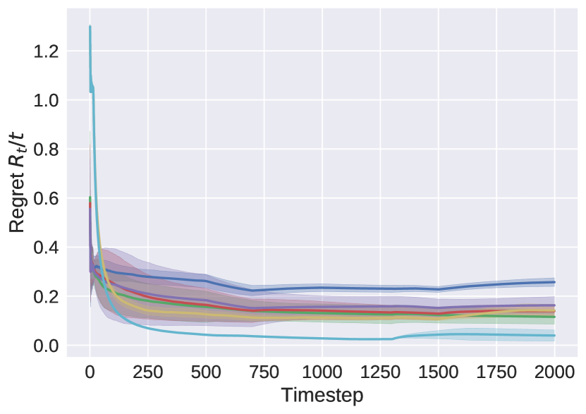
(a) Sine

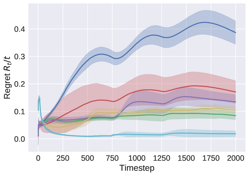
(b) Gaussian

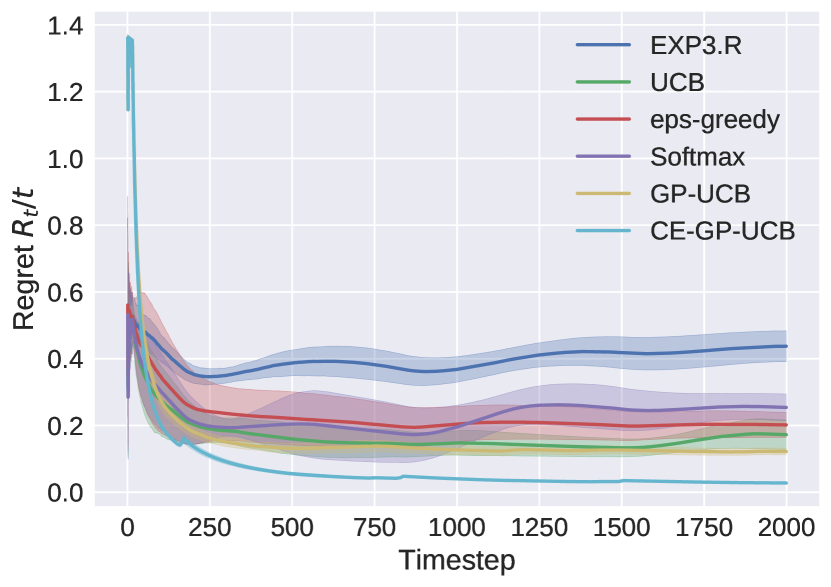
(c) Piecewise

Figure A2: Average regret $R_{T}/T$ for time-varying bandits algorithms on three different synthetic data.

As shown in Table A1, we found proposed CE-GP-UCB consistently achieves lower regrets while interacting less with the unknown functions. This is because CE-GP-UCB automatically assesses the confidence of current policy based on current GP models and given problems, and skips the queries if it is pretty confident the decision is correct. Moreover, compared to GP-UCB with full observations, our method saves around 97.5% queries, which results in $40\times$ computation cost saving in evaluating the unknown objective. Figure A2 shows how $R_{t}/t$ evolves as training proceeds for different algorithms. It again verifies cost-efficient query rule can adapt to different problems quickly and achieve lower regrets.

TV Bayesian optimization

Table A2 presents numerical performance of CE-GP-UCB on synthetic data with different confidence threshold $\kappa$. The performance is averaged over 50 independent trials. We found that CE-GP-UCB can almost recover the performance of original TV-GP-UCB meanwhile significantly cutting off the cost for interacting with unknown functions which is usually very expensive. Taking $\epsilon=0.05$ for instance, CE-GP-UCB ($\kappa=0.9$) reduces up to 40% queries meanwhile only suffers from 2.6% regret loss.

Table A2: Numerical performance on synthetic data. $R_{T}/T$ and $C_{T}$ denote average regret and total cost for observing rewards. @$\kappa$ denotes the confidence threshold for CE-GP-UCB is $\kappa$. @* denotes the LCB-UCB rule (Lemma 1). We highlight the setting within 10% regret loss compared to TV-GP-UCB with full observations. The performance is averaged over 50 independent trials.

	$\epsilon=0.003$		$\epsilon=0.005$		$\epsilon=0.01$		$\epsilon=0.03$		$\epsilon=0.05$
	$R_{T}/T$	$C_{T}$	$R_{T}/T$	$C_{T}$	$R_{T}/T$	$C_{T}$	$R_{T}/T$	$C_{T}$	$R_{T}/T$	$C_{T}$
R-GP-UCB	$0.352\pm 0.187$	$499\pm 0$	$0.371\pm 0.166$	$499\pm 0$	$0.425\pm 0.118$	$499\pm 0$	$0.516\pm 0.093$	$499\pm 0$	$0.581\pm 0.093$	$499\pm 0$
TV-GP-UCB	$0.094\pm 0.035$	$499\pm 0$	$0.126\pm 0.044$	$499\pm 0$	$0.184\pm 0.056$	$499\pm 0$	$0.305\pm 0.034$	$499\pm 0$	$0.392\pm 0.034$	$499\pm 0$
TV-GP-UCB Ber(0.2)	$0.231\pm 0.089$	$99\pm 8$	$0.275\pm 0.084$	$99\pm 9$	$0.350\pm 0.094$	$97\pm 9$	$0.561\pm 0.122$	$100\pm 9$	$0.694\pm 0.090$	$100\pm 8$
TV-GP-UCB Ber(0.3)	$0.176\pm 0.093$	$147\pm 9$	$0.218\pm 0.104$	$150\pm 12$	$0.312\pm 0.089$	$144\pm 10$	$0.485\pm 0.089$	$150\pm 10$	$0.592\pm 0.096$	$153\pm 10$
TV-GP-UCB Ber(0.4)	$0.147\pm 0.072$	$200\pm 10$	$0.186\pm 0.073$	$200\pm 10$	$0.275\pm 0.090$	$201\pm 11$	$0.428\pm 0.073$	$203\pm 11$	$0.522\pm 0.073$	$203\pm 9$
TV-GP-UCB Ber(0.5)	$0.121\pm 0.060$	$247\pm 10$	$0.160\pm 0.061$	$249\pm 12$	$0.241\pm 0.073$	$252\pm 12$	$0.382\pm 0.064$	$249\pm 12$	$0.480\pm 0.058$	$250\pm 12$
TV-GP-UCB Ber(0.6)	$0.119\pm 0.055$	$296\pm 9$	$0.144\pm 0.041$	$300\pm 11$	$0.230\pm 0.078$	$298\pm 11$	$0.363\pm 0.045$	$298\pm 11$	$0.452\pm 0.045$	$298\pm 12$
TV-GP-UCB Ber(0.7)	$0.112\pm 0.049$	$348\pm 10$	$0.151\pm 0.060$	$348\pm 11$	$0.209\pm 0.068$	$348\pm 10$	$0.335\pm 0.038$	$350\pm 11$	$0.429\pm 0.040$	$350\pm 9$
TV-GP-UCB Ber(0.8)	$0.102\pm 0.046$	$401\pm 9$	$0.140\pm 0.058$	$399\pm 11$	$0.198\pm 0.067$	$399\pm 9$	$0.328\pm 0.035$	$400\pm 8$	$0.415\pm 0.037$	$400\pm 7$
TV-GP-UCB Ber(0.9)	$0.098\pm 0.048$	$450\pm 7$	$0.132\pm 0.051$	$449\pm 7$	$0.196\pm 0.066$	$448\pm 7$	$0.311\pm 0.036$	$448\pm 6$	$0.404\pm 0.035$	$449\pm 7$
CE-GP-UCB @0.60	$0.535\pm 0.416$	$8\pm 5$	$0.558\pm 0.319$	$12\pm 7$	$0.600\pm 0.289$	$20\pm 11$	$0.642\pm 0.141$	$53\pm 11$	$0.680\pm 0.119$	$85\pm 17$
CE-GP-UCB @0.70	$0.410\pm 0.329$	$16\pm 11$	$0.435\pm 0.253$	$21\pm 13$	$0.442\pm 0.186$	$41\pm 25$	$0.504\pm 0.096$	$91\pm 21$	$0.533\pm 0.071$	$134\pm 21$
CE-GP-UCB @0.75	$0.341\pm 0.249$	$22\pm 17$	$0.367\pm 0.199$	$34\pm 20$	$0.368\pm 0.176$	$62\pm 27$	$0.441\pm 0.077$	$117\pm 25$	$0.484\pm 0.074$	$167\pm 30$
CE-GP-UCB @0.80	$0.286\pm 0.169$	$31\pm 27$	$0.297\pm 0.157$	$51\pm 36$	$0.304\pm 0.117$	$76\pm 27$	$0.387\pm 0.065$	$146\pm 31$	$0.451\pm 0.053$	$200\pm 30$
CE-GP-UCB @0.85	$0.226\pm 0.131$	$51\pm 41$	$0.248\pm 0.095$	$78\pm 42$	$0.266\pm 0.069$	$101\pm 46$	$0.356\pm 0.054$	$180\pm 34$	$0.416\pm 0.041$	$235\pm 35$
CE-GP-UCB @0.90	$0.188\pm 0.089$	$82\pm 73$	$0.202\pm 0.080$	$101\pm 63$	$0.238\pm 0.070$	$140\pm 48$	$0.322\pm 0.045$	$233\pm 37$	$0.400\pm 0.036$	$291\pm 30$
CE-GP-UCB @0.95	$0.157\pm 0.074$	$125\pm 77$	$0.161\pm 0.051$	$163\pm 73$	$0.210\pm 0.052$	$207\pm 60$	$0.307\pm 0.037$	$310\pm 42$	$0.397\pm 0.034$	$371\pm 29$
CE-GP-UCB @0.99	$0.112\pm 0.037$	$292\pm 104$	$0.128\pm 0.030$	$309\pm 83$	$0.176\pm 0.031$	$363\pm 60$	$0.295\pm 0.031$	$435\pm 26$	$0.386\pm 0.033$	$468\pm 15$
CE-GP-UCB @*	$0.103\pm 0.034$	$386\pm 79$	$0.126\pm 0.031$	$414\pm 50$	$0.168\pm 0.033$	$442\pm 41$	$0.292\pm 0.031$	$482\pm 11$	$0.384\pm 0.031$	$492\pm 7$

B.2 Self-Tuning Networks

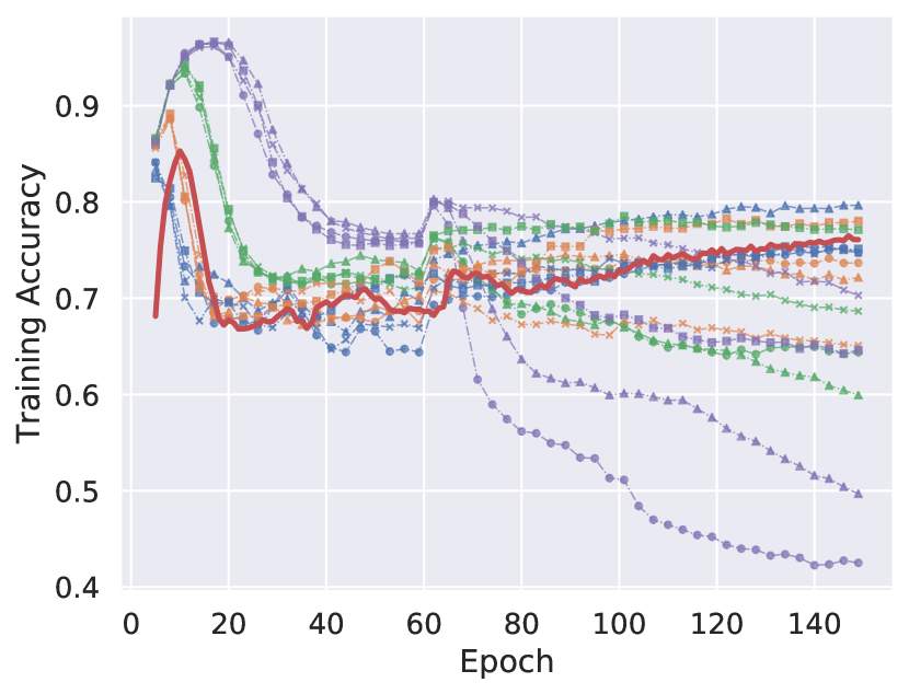
(a) Training Accuracy

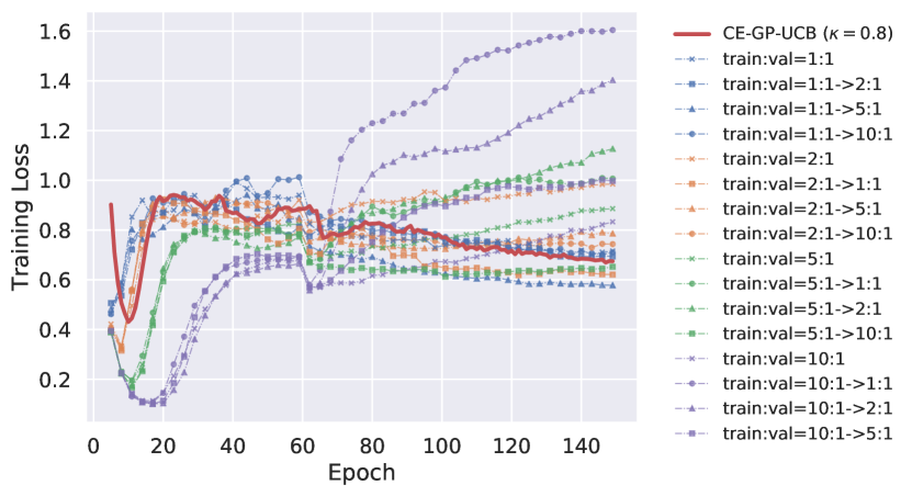
(b) Training Loss

Figure A3: Learning curves on (a) training accuracy & (b) training loss under different tuning schedules. Note that the training curves for STN is different form standard training since at the late stage of training, large amounts of data augmentations are added to avoid overfitting. Our proposed CE-GP-UCB finds an unique pattern that differs from static tuning schedules or switching schedules automatically.

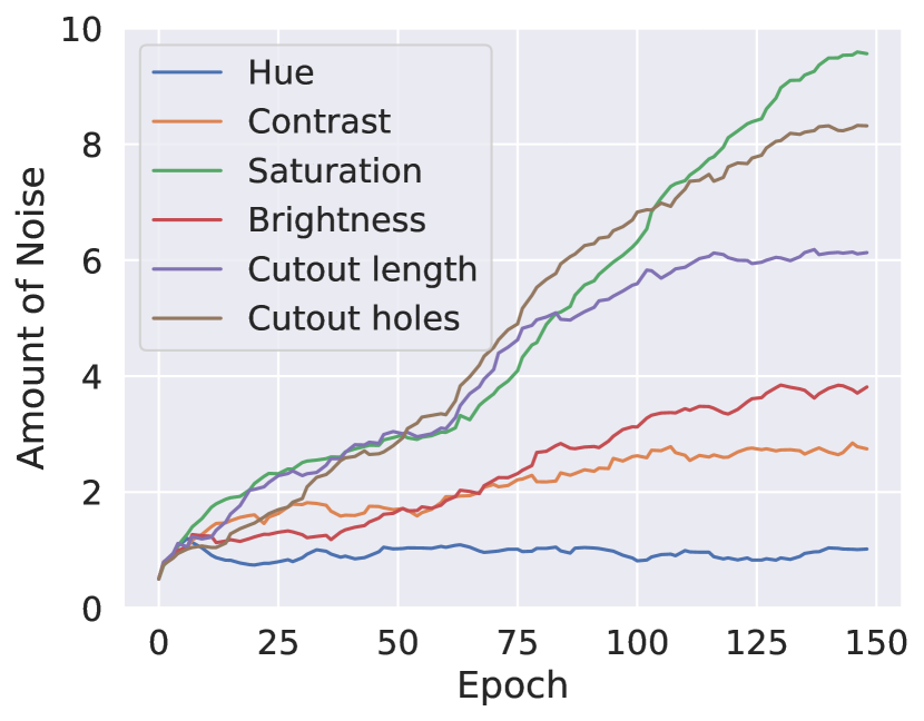
(a) train/val=1:1

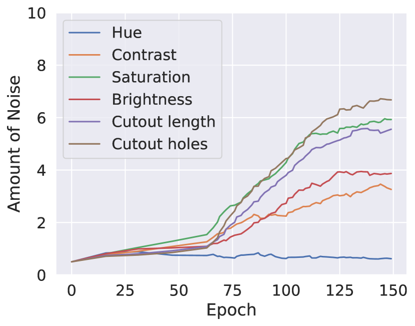
(b) train/val=10:1-¿1:1

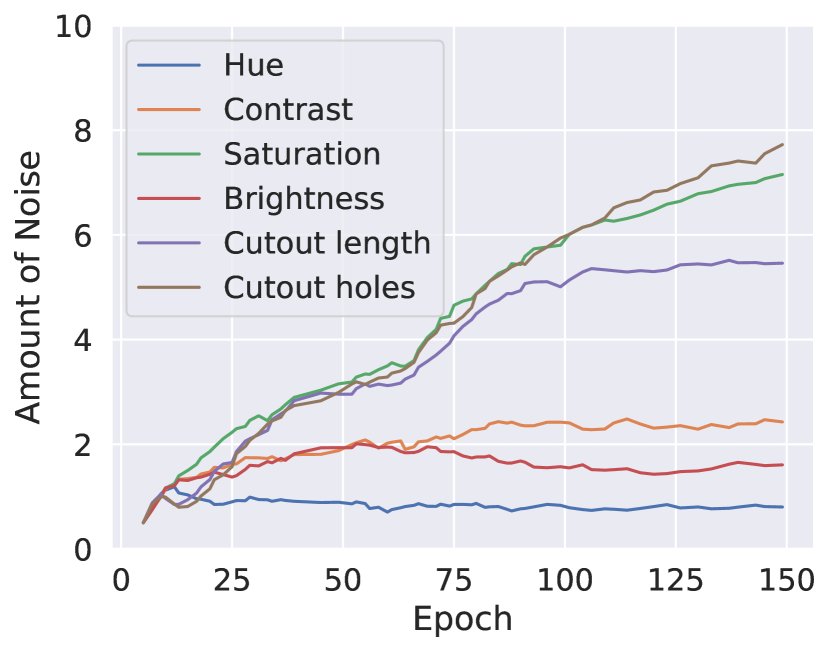
(c) CE-GP-UCB (ours)

Figure A4: The hyperparameter schedule prescribed by the STN (VGG16 on CIFAR-10).

Figure A3 shows the training curves (loss and accuracy) under different tuning schedules. We observed that the training curves of STN differ from standard training curves since large amounts of data augmentations are added at the late stage of training which results in a huge performance loss on training data. However, even though the performance is significantly worse on the training set (e.g., 60% to 80% training accuracy), the model still performs well on the clean images without augmentations on the validation set and test set (see Figure 3).

Figure A4 presents the hyperparameter schedule prescribed by the STN under different tuning schedules. In general, the amount of noise added to the image increases as the training proceeds to alleviate the effects of overfitting. However, we found that CE-GP-UCB results in a slightly different pattern. Specifically, STN decreases the brightness at the late training stage with CE-GP-UCB, however, it increases the brightness as other data augmentations under static or switching tuning schedules.

B.3 Unsupervised Contrastive Representation Learning

Implementation Details for SimCLR

Following Chen et al. (2020), we take ResNet-50 (He et al., 2016) as the encoder network, and a 2-layer MLP projection head to project the representation. We trained SimCLR with 64 GPUs on ImageNet100 (Tian et al., 2019) (100 classes of ImageNet) for 200 epochs and set the batch-size as $64\times 56=3584$. To stabilize the training with large batch size, the LARS optimizer is adopted with the learning rate $4.8$. For linear readout evaluation, a linear layer is trained from scratch for 10 epochs. We adopt SGD optimizer with a learning rate of 10 and momentum 0.9 following Tian et al. (2019).

Implementation Details for CE-GP-UCB

We integrate CE-GP-UCB algorithm into the popular botorch library (Balandat et al., 2019) for higher efficiency and stable performance. Specifically, we use Matern5/2 and set the forgetting rate as $\epsilon=0.01$. To find all the local optima, we randomly initialize 50 locations and use L-BFGS algorithm (Liu and Nocedal, 1989) to find the local optima. Furthermore, we use meanshift (Cheng, 1995) algorithm to suppress close candidates with a bandwidth of 0.2. To avoid catastrophic performance loss and misleading signals by some extremely biased decision, we clip the reward signals between $[-2,2]$ and set the minimal probability to apply the cropping as 0.5.

References

- Auer et al. (2002a) Peter Auer, Nicolo Cesa-Bianchi, and Paul Fischer. Finite-time analysis of the multiarmed bandit problem. Machine learning, 47(2-3):235–256, 2002a.
- Auer et al. (2002b) Peter Auer, Nicolo Cesa-Bianchi, Yoav Freund, and Robert E Schapire. The nonstochastic multiarmed bandit problem. SIAM journal on computing, 32(1):48–77, 2002b.
- Balandat et al. (2019) Maximilian Balandat, Brian Karrer, Daniel R. Jiang, Samuel Daulton, Benjamin Letham, Andrew Gordon Wilson, and Eytan Bakshy. Botorch: Programmable bayesian optimization in pytorch. CoRR, abs/1910.06403, 2019.
- Bergstra and Bengio (2012) James Bergstra and Yoshua Bengio. Random search for hyper-parameter optimization. Journal of machine learning research, 13(Feb):281–305, 2012.
- Bergstra et al. (2011) James Bergstra, Rémi Bardenet, Yoshua Bengio, and Balázs Kégl. Algorithms for hyper-parameter optimization. In NIPS, pages 2546–2554, 2011.
- Bertrand et al. (2020) Quentin Bertrand, Quentin Klopfenstein, Mathieu Blondel, Samuel Vaiter, Alexandre Gramfort, and Joseph Salmon. Implicit differentiation of lasso-type models for hyperparameter optimization. CoRR, abs/2002.08943, 2020.
- Bogunovic et al. (2016) Ilija Bogunovic, Jonathan Scarlett, and Volkan Cevher. Time-varying gaussian process bandit optimization. In AISTATS, volume 51 of JMLR Workshop and Conference Proceedings, pages 314–323. JMLR.org, 2016.
- Bogunovic et al. (2018) Ilija Bogunovic, Jonathan Scarlett, Stefanie Jegelka, and Volkan Cevher. Adversarially robust optimization with gaussian processes. In Conference on Neural Information Processing Systems (NeurIPS), 2018.
- Chen et al. (2020) Ting Chen, Simon Kornblith, Mohammad Norouzi, and Geoffrey E. Hinton. A simple framework for contrastive learning of visual representations. CoRR, abs/2002.05709, 2020.
- Cheng (1995) Yizong Cheng. Mean shift, mode seeking, and clustering. IEEE Trans. Pattern Anal. Mach. Intell., 17(8):790–799, 1995.
- Deng et al. (2009) Jia Deng, Wei Dong, Richard Socher, Li-Jia Li, Kai Li, and Fei-Fei Li. Imagenet: A large-scale hierarchical image database. In CVPR, pages 248–255. IEEE Computer Society, 2009.
- Desautels et al. (2014) Thomas Desautels, Andreas Krause, and Joel W. Burdick. Parallelizing exploration-exploitation tradeoffs in gaussian process bandit optimization. Journal of machine learning research, 15(1):3873–3923, 2014.
- Domke (2012) Justin Domke. Generic methods for optimization-based modeling. In AISTATS, volume 22 of JMLR Proceedings, pages 318–326. JMLR.org, 2012.
- Franceschi et al. (2018) Luca Franceschi, Paolo Frasconi, Saverio Salzo, Riccardo Grazzi, and Massimiliano Pontil. Bilevel programming for hyperparameter optimization and meta-learning. In ICML, volume 80 of Proceedings of Machine Learning Research, pages 1563–1572. PMLR, 2018.
- Ha et al. (2017) David Ha, Andrew M. Dai, and Quoc V. Le. Hypernetworks. In ICLR (Poster). OpenReview.net, 2017.
- He et al. (2016) Kaiming He, Xiangyu Zhang, Shaoqing Ren, and Jian Sun. Deep residual learning for image recognition. In CVPR, pages 770–778. IEEE Computer Society, 2016.
- Hutter et al. (2011) Frank Hutter, Holger H. Hoos, and Kevin Leyton-Brown. Sequential model-based optimization for general algorithm configuration. In LION, volume 6683 of Lecture Notes in Computer Science, pages 507–523. Springer, 2011.
- Imamura et al. (2020) Hideaki Imamura, Nontawat Charoenphakdee, Futoshi Futami, Issei Sato, Junya Honda, and Masashi Sugiyama. Time-varying gaussian process bandit optimization with non-constant evaluation time. CoRR, abs/2003.04691, 2020.
- Jamieson and Talwalkar (2016) Kevin G. Jamieson and Ameet Talwalkar. Non-stochastic best arm identification and hyperparameter optimization. In AISTATS, volume 51 of JMLR Workshop and Conference Proceedings, pages 240–248. JMLR.org, 2016.
- Klein et al. (2017a) Aaron Klein, Stefan Falkner, Simon Bartels, Philipp Hennig, and Frank Hutter. Fast bayesian optimization of machine learning hyperparameters on large datasets. In AISTATS, volume 54 of Proceedings of Machine Learning Research, pages 528–536. PMLR, 2017a.
- Klein et al. (2017b) Aaron Klein, Stefan Falkner, Jost Tobias Springenberg, and Frank Hutter. Learning curve prediction with bayesian neural networks. In ICLR (Poster). OpenReview.net, 2017b.
- Krause and Ong (2011) Andreas Krause and Cheng Soon Ong. Contextual gaussian process bandit optimization. In NIPS, pages 2447–2455, 2011.
- Krizhevsky et al. (2009) Alex Krizhevsky, Geoffrey Hinton, et al. Learning multiple layers of features from tiny images. 2009.
- Kuleshov and Precup (2000) Volodymyr Kuleshov and Doina Precup. Algorithms for the multi-armed bandit problem. In Journal of machine learning research. Citeseer, 2000.
- Lam et al. (2016) Rémi Lam, Karen Willcox, and David H. Wolpert. Bayesian optimization with a finite budget: An approximate dynamic programming approach. In NIPS, pages 883–891, 2016.
- Larsen et al. (1996) Jan Larsen, Lars Kai Hansen, Claus Svarer, and M Ohlsson. Design and regularization of neural networks: the optimal use of a validation set. In Neural Networks for Signal Processing VI. Proceedings of the 1996 IEEE Signal Processing Society Workshop, pages 62–71. IEEE, 1996.
- Li et al. (2017) Lisha Li, Kevin G. Jamieson, Giulia DeSalvo, Afshin Rostamizadeh, and Ameet Talwalkar. Hyperband: Bandit-based configuration evaluation for hyperparameter optimization. In ICLR (Poster). OpenReview.net, 2017.
- Liu and Nocedal (1989) Dong C. Liu and Jorge Nocedal. On the limited memory BFGS method for large scale optimization. Math. Program., 45(1-3):503–528, 1989.
- Lorraine and Duvenaud (2018) Jonathan Lorraine and David Duvenaud. Stochastic hyperparameter optimization through hypernetworks. CoRR, abs/1802.09419, 2018.
- Lorraine et al. (2019) Jonathan Lorraine, Paul Vicol, and David Duvenaud. Optimizing millions of hyperparameters by implicit differentiation. CoRR, abs/1911.02590, 2019.
- Luketina et al. (2016) Jelena Luketina, Tapani Raiko, Mathias Berglund, and Klaus Greff. Scalable gradient-based tuning of continuous regularization hyperparameters. In ICML, volume 48 of JMLR Workshop and Conference Proceedings, pages 2952–2960. JMLR.org, 2016.
- MacKay et al. (2019) Matthew MacKay, Paul Vicol, Jonathan Lorraine, David Duvenaud, and Roger B. Grosse. Self-tuning networks: Bilevel optimization of hyperparameters using structured best-response functions. In ICLR (Poster). OpenReview.net, 2019.
- Nguyen et al. (2019) Vu Nguyen, Sebastian Schulze, and Michael A. Osborne. Bayesian optimization for iterative learning. CoRR, abs/1909.09593, 2019.
- Pedregosa (2016) Fabian Pedregosa. Hyperparameter optimization with approximate gradient. In ICML, volume 48 of JMLR Workshop and Conference Proceedings, pages 737–746. JMLR.org, 2016.
- Shahriari et al. (2015) Bobak Shahriari, Kevin Swersky, Ziyu Wang, Ryan P Adams, and Nando De Freitas. Taking the human out of the loop: A review of bayesian optimization. Proceedings of the IEEE, 104(1):148–175, 2015.
- Snoek et al. (2012) Jasper Snoek, Hugo Larochelle, and Ryan P. Adams. Practical bayesian optimization of machine learning algorithms. In NIPS, pages 2960–2968, 2012.
- Snoek et al. (2015) Jasper Snoek, Oren Rippel, Kevin Swersky, Ryan Kiros, Nadathur Satish, Narayanan Sundaram, Md. Mostofa Ali Patwary, Prabhat, and Ryan P. Adams. Scalable bayesian optimization using deep neural networks. In ICML, volume 37 of JMLR Workshop and Conference Proceedings, pages 2171–2180. JMLR.org, 2015.
- Srinivas et al. (2010) Niranjan Srinivas, Andreas Krause, Sham M. Kakade, and Matthias W. Seeger. Gaussian process optimization in the bandit setting: No regret and experimental design. In ICML, pages 1015–1022. Omnipress, 2010.
- Swersky et al. (2014) Kevin Swersky, Jasper Snoek, and Ryan Prescott Adams. Freeze-thaw bayesian optimization. CoRR, abs/1406.3896, 2014.
- Tian et al. (2019) Yonglong Tian, Dilip Krishnan, and Phillip Isola. Contrastive multiview coding. CoRR, abs/1906.05849, 2019.